Discrete Fourier Transform versus Discrete Chi-Square Method

Abstract

We compare two time series analysis methods, the Discrete Fourier Transform (DFT) and our Discrete Chi-square Method (DCM). DCM is designed for detecting many signals superimposed on an unknown trend. The solution for the non-linear DCM model is an ill-posed problem. The backbone of DCM is the Gauss-Markov theorem that the least squares fit is the best unbiased estimator for linear regression models. DCM is a simple numerical time series analysis method that performs a massive number of linear least squares fits. We show that our numerical solution for the DCM model fulfills the three conditions of a well-posed problem: existence, uniqueness and stability. The Fisher-test is used to identify the best DCM model from all alternative tested DCM models. The correct DCM model must also pass our Predictivity-test. Our analyses of seven different simulated data samples expose the weaknesses of DFT and the efficiency of DCM. The DCM signal and trend detection depend only on the sample size and the accuracy of data. DCM is an ideal forecasting method because the time span of observations is irrelevant. We recommend fast sampling of large high quality datasets and the analysis of those datasets using numerical DCM parallel computation Python code.

1 Introduction

[9] defined the three conditions for a well-posed problem. The solution for the problem determines these conditions.

• $\mathrm{C}_{1}$ Existence: A solution exists.

• $\mathrm{C}_{2}$ Uniqueness: The solution is unique.

• $\mathrm{C}_{3}$ Stability: Small changes in the input data cause small changes in the solution.

Stability means that the solution behaves predictably as the input varies. In other words, there exists a continuous mapping from the input space to the solution space.

If any of these conditions are not satisfied, the problem is classified as ill-posed. Ill-posed problems are encountered in various fields of science [22]. For example, Piskunov et al. [24] solves the stellar surface imaging inverse problem using the [29] regularization technique. Ill-posed problems are also encountered in time series analysis of astronomical data [30, 1]. The problem is ill-posed because the unknown signal frequencies are free parameters of non-linear time series analysis models. The Lomb-Scargle periodogram is the most frequently applied time series analysis method in astronomy because the observations are often unevenly spaced in time [21, 27]. Several extentions of this method have been published [35, 32]. The DFT pre-whitening technique can detect many signals from unevenly spaced data [e.g., 26, 34]. The data must be detrended before applying this technique, which detects one frequency at a time, until it detects no new frequency. In this study, artificial simulated data having equal weights is analysed using the DFT version published by Horne and Baliunas [11]. We compare the performance of this DFT version to the performance of our DCM.

[19] formulated the least squares method. [7] connected this method to the principles of probability and the normal distribution. A few years later, he showed that the least-squares method gives the best unbiased estimates for the free parameters of linear models, if the zero mean data errors are equal, normally distributed and uncorrelated [8]. The extended Gauss-Markov theorem states that the least squares method gives the best estimates for the free parameters of linear models, even if the data errors do not pass all the above-mentioned criteria [33]. This Gauss-Markov theorem is the backbone of our DCM.

We present the DCM formulation in Section 2.1. Data samples are simulated using the DCM model (Sect. 2.2). The four DFT limitations are discussed in Section 2.3 (Equations 26-29). DCM and DFT time series analysis of the simulated data samples shows that DCM does not suffer from the DFT limitations (Sects. 3.1-3.7). We then present the identification of the best DCM model for the data (Sect. 3.8), the DCM significance estimates (Sect. 3.9) and the DCM predictions (Sect. 3.10). Finally, we discuss our results (Sect. 4).

2 Methods

The observations are $y_{i}=y(t_{i})\pm\sigma(t_{i})$, where $t_{i}$ are the observing times and $\sigma_{i}$ are the errors $(i=1,2,...,n)$. The time span of data is $\Delta T=t_{n}-t_{1}$. The mid point is $t_{\mathrm{mid}}=t_{1}+\Delta T/2$. The mean and the standard deviation of all $y_{i}$ values are denoted with $m$ and $s$.

2.1 Discrete Chi-square method (DCM)

[13] formulated DCM. The model of this method is

$$g(t)=g(t,K_{1},K_{2},K_{3})=h(t)+p(t),$$ (1)

where the integer values $K_{1}$, $K_{2}$ and $K_{3}$ are called the model orders [14]. The notation $g_{K_{1},K_{2},K_{3}}(t)$ is used to specify these orders. The DCM model is a sum of two functions. These functions are the periodic function

$$h(t) = h(t,K_{1},K_{2})=\sum_{i=1}^{K_{1}}h_{i}(t,f_{i})$$ (2)

$$h_{i}(t,f_{i}) = \sum_{j=1}^{K_{2}}B_{i,j}\cos{(2\pi jf_{i}t)}$$

$$+ C_{i,j}\sin{(2\pi jf_{i}t)}$$

and the aperiodic function

$$p(t)=p(t,K_{3})=\begin{cases}0,&\text{if }K_{3}=-1\\ \sum_{k=0}^{K_{3}}p_{k}(t),&\text{if }K_{3}=0,1,2,...\end{cases}$$ (4)

where

$$p_{k}(t) = M_{k}\left[{{2(t-t_{\mathrm{mid}}})\over{\Delta T}}\right]^{k}.$$ (5)

For $k>1$, the $p_{k}(t)$ function full range is

$$\begin{cases}2|M_{k}|,&\text{if $k$ is odd}\\ |M_{k}|,&\text{if $k$ is even.}\end{cases}$$ (6)

The free parameters of $g(t)$ model are

$$\bm{\beta} = [\beta_{1},\beta_{2},...,\beta_{\eta}]$$

$$= [B_{1,1},C_{1,1},f_{1},...,B_{K_{1},K_{2}},C_{K_{1},K_{2}},f_{K_{1}},M_{0},...,M_{K_{3}}].$$

The number of free parameters is

$$\eta=K_{1}\times(2K_{2}+1)+K_{3}+1.$$ (8)

We divide the free parameters $\bm{\beta}$ into two groups $\bm{\beta}_{I}$ and $\bm{\beta}_{II}$. The first group are the frequencies

$$\bm{\beta}_{I} = [f_{1},...,f_{K_{1}}].$$ (9)

Due to this group, all free parameters are not eliminated from all partial derivatives $\partial g/\partial\beta_{i}$. This makes the $g(t)$ model non-linear. If the $\bm{\beta}_{I}$ frequencies have constant values, the multipliers $2\pi jf_{i}$ in Equation 2.1 become constants. In this case, the model becomes linear because the partial derivatives $\partial g/\partial\beta_{i}$ no longer contain any free parameters. The solution for the second group of remaining free parameters

$$\bm{\beta}_{II} = [B_{1,1}C_{1,1},...,B_{K_{1},K_{2}},C_{K_{1},K_{2}},M_{0},...,M_{K_{3}}]$$ (10)

becomes unique. This solution passes the $\mathrm{C}_{1}$, $\mathrm{C}_{2}$ and $\mathrm{C}_{3}$ conditions of a well-posed problem.

Let us assume that we search for periods between $f_{\mathrm{min}}$ and $f_{\mathrm{max}}$. The non-linear $g(t)$ model becomes linear, if the tested $\bm{\beta}_{I}$ frequencies are fixed to any constant values. The sum $h(t)$ of signals $h_{1}(t,f_{1})$, $h_{2}(t,f_{2})$ … and $h_{K_{1},f_{K_{1}}}(t)$ does not depend on the order in which these signals are added. For example, the two signal $K_{1}=2$ model symmetry is $h(t)=h_{1}(t,f_{1})+h_{2}(t,f_{2})=h_{1}(t,f_{2})+h_{2}(t,f_{1})$. Both $(f_{1},f_{2})$ and $(f_{2},f_{1})$ combinations give the same value for the $g(t)$ model. Since this symmetry applies to any $K_{1}$ number of signals, we compute the linear $g(t)$ models only for all tested frequency combinations

$$f_{\mathrm{max}}\geq f_{1}>f_{2}>...>f_{K_{1}}\geq f_{\mathrm{min}}.$$ (11)

The DCM model residuals

$$\epsilon_{i}=y(t_{i})-g(t_{i})=y_{i}-g_{i}.$$ (12)

give the sum of squared residuals

$$R=\sum_{i=1}^{n}\epsilon_{i}^{2},$$ (13)

and the Chi-square

$$\chi^{2}=\sum_{i=1}^{n}{{\epsilon_{i}^{2}}\over{\sigma_{i}^{2}}}.$$ (14)

For every tested $\bm{\beta}_{I}=[f_{1},f_{2},...,f_{K_{1}}]$ frequency combination, the DCM test statistic

$$z = z(f_{1},f_{2},...,f_{K_{1}})=\sqrt{R/n}$$ (15)

$$z = z(f_{1},f_{2},...,f_{K_{1}})=\sqrt{\chi^{2}/n}$$ (16)

is computed from a linear model least squares fit. Equation 15 or Equation 16 is applied for unknown or known $\sigma_{i}$ errors, respectively. The value of $z$ is unique.

In the preliminary long search, we test an evenly spaced grid of $n_{\mathrm{L}}$ frequencies between $f_{\mathrm{min}}$ and $f_{\mathrm{max}}$. This search gives the best frequency candidates $f_{\mathrm{1,mid}},...f_{\mathrm{K_{1},mid}}$.

In the final short search, we test a denser grid of $n_{\mathrm{S}}$ frequencies within an interval

$$[f_{\mathrm{i,mid}}-a,f_{\mathrm{i,mid}}+a],$$ (17)

where $i=1,..,K_{1}$, $a=c(f_{\mathrm{min}}-f_{\mathrm{max}})/2$ and $c=0.05$.

The total number of all tested long and short search frequency combinations is

$$\binom{n_{f}}{K_{1}}={{n_{f}!}\over{K_{1}!(n_{f}-K_{1})!}},$$ (18)

where $n_{f}=n_{L}$ and $n_{f}=n_{S}$, respectively.

The global periodogram minimum

$$z_{\mathrm{min}}=z(f_{\mathrm{1,best}},f_{\mathrm{2,best}},...,f_{\mathrm{K_{1},best}})$$ (19)

is at the tested frequencies $f_{\mathrm{1,best}},$ $f_{\mathrm{2,best}},...,$ $f_{\mathrm{K_{1},best}}$. This tested frequency combination gives the best linear model for the data. The periodogam value $z$ is a scalar, which is computed from $K_{1}$ frequency values. It is possible to plot the $K_{1}=2$ two signal periodogram $z(f_{1},f_{2})$ as a map, where $f_{1}$ and $f_{2}$ are the coordinates, and $z=z(f_{1},f_{2})$ is the height. For more than two signals, there is no direct graphical $z$ plot because that requires more than three dimensions. Our solution for this dimensional problem is simple. We plot only the following one-dimensional slices of the full periodogram

$$z_{1}(f_{1}) = z(f_{1},f_{\mathrm{2,best}},...,f_{\mathrm{K_{1},best}})$$ (20)

$$z_{2}(f_{2}) = z(f_{\mathrm{1,best}},f_{2},f_{\mathrm{3,best}},...,f_{\mathrm{K_{1},best}})$$

$$z_{3}(f_{3}) = z(f_{\mathrm{1,best}},f_{\mathrm{2,best}},f_{3},f_{\mathrm{4,best}},...,f_{\mathrm{K_{1},best}})~$$

$$z_{4}(f_{4}) = z(f_{\mathrm{1,best}},f_{\mathrm{2,best}},f_{\mathrm{3,best}},f_{4},f_{\mathrm{5,best}},f_{\mathrm{K_{1},best}})$$

$$z_{5}(f_{5}) = z(f_{\mathrm{1,best}},f_{\mathrm{2,best}},f_{\mathrm{3,best}},f_{\mathrm{4,best}},f_{5},f_{\mathrm{K_{1},best}})$$

$$z_{6}(f_{6}) = z(f_{\mathrm{1,best}},f_{\mathrm{2,best}},f_{\mathrm{3,best}},f_{\mathrm{4,best}},f_{\mathrm{5,best}},f_{6}).$$

In the above-mentioned $K_{1}=2$ map, the slice $z_{1}(f_{1})$ would represent the height $z$ at the location $(f_{1},f_{\mathrm{2,best}})$ when moving along the straight constant line $f_{2}=f_{\mathrm{2,best}}$ that crosses the global minimum $z_{\mathrm{min}}$ (Equation 19) at the coordinate point $(f_{\mathrm{1,best}},f_{\mathrm{2,best}})$.

The short search gives the best $f_{\mathrm{1,best}},...,$ $f_{\mathrm{K_{1},best}}$ frequencies for the data. These frequencies are the unique initial values for the first group of free parameters $\bm{\beta}_{\mathrm{I,initial}}=$ $[f_{\mathrm{1,best}},...,$ $f_{\mathrm{K_{1},best}}]$ (Equation 9). The linear model for these constant $[f_{\mathrm{1,best}},...,f_{\mathrm{K_{1},best}}]$ frequencies gives the unique initial values for the second group $\bm{\beta}_{\mathrm{II,initial}}$ of free parameters (Equation 10). The non-linear iteration

$$\bm{\beta}_{\mathrm{initial}}=[\bm{\beta}_{\mathrm{I,initial}},\bm{\beta}_{\mathrm{II,initial}}]\rightarrow\bm{\beta}_{\mathrm{final}}$$ (21)

gives the final free parameter values $\bm{\beta}_{\mathrm{final}}$.

DCM determines the signal parameters

• $P_{i}=1/f_{i}=$ Period

• $A_{i}=$ Peak to peak amplitude

• $t_{\mathrm{i,min,1}}=$ Deeper primary minimum

• $t_{\mathrm{i,min,2}}=$ Secondary minimum (if present)

• $t_{\mathrm{i,max,1}}=$ Higher primary maximum

• $t_{\mathrm{i,max,2}}=$ Secondary maximum (if present)

and the trend parameters

• $M_{k}$ = Polynomial coeffients.

We use the bootstrap technique to estimate the DCM model parameter errors [5]. The tested bootstrap frequencies are the same as in the short search. Our TSPA- and CPS-methods applied the same bootstrap tehnique [15, 20]. We select a random sample $\bm{\epsilon}^{*}$ from the residuals $\bm{\epsilon}$ of the DCM model (Equation 12). Any $\epsilon_{i}$ value can be chosen to the $\bm{\epsilon}^{*}$ sample as many times as the random selection happens to favour it. We create numerous artificial bootstrap data samples

$$\bm{y}^{*}=\bm{g}+\bm{\epsilon}^{*}.$$ (22)

Each $\bm{y}^{*}$ sample gives one estimate for every DCM model parameter. For each particular model parameter, the bootstrap error estimate is the standard deviation of all estimates obtained from all $\bm{y}^{*}$ samples.

There are, of course, totally wrong DCM models for the data. For example, DCM can be forced search for too few or too many $K_{1}$ signals, or the selected $p(t)$ trend order $K_{3}$ can be wrong, as shown in Figures 5-10 by [13]. Such DCM models are unstable and we denote them with “${\color[rgb]{0,0,0}{\bf\mathrm{UM}}}$”, like in [14] and Jetsu (2025). These unstable models have three signatures

• Intersecting frequencies

• Dispersing amplitudes

• Leaking periods

Intersecting frequencies occur when the signal frequencies in the data are very close to each other. We give the following example of how this instability can arise in the two signal model. If the frequency $f_{1}$ approaches the frequency $f_{2}$, both $h_{1}(t)$ and $h_{2}(t)$ signals become essentially one and the same signal. The least squares fit fails because it makes no sense to model the same signal twice.

Dispersing amplitudes instability can occur, if the two signal frequencies are too close to each other. The least squares fit finds a model, where two high amplitude signals nearly cancel out each other. The low amplitude signal, the sum of these two high amplitude signals, fits to the data.

There are DCM models where the detected frequency $f$ is outside the tested frequency interval between $f_{\mathrm{min}}$ and $f_{\mathrm{max}}$. This leaking periods instability may indicate that the chosen tested period range is wrong.

Table 1: Model 1: DCM analysis between $P_{\mathrm{min}}=0.63$ and $P_{\mathrm{max}}=5.70$. (1) Simulated $P_{1}$, $A_{1}$, $t_{\mathrm{1,min,1}}$, $t_{\mathrm{1,max,1}}$ and $M_{0}$ values. (2-4) Detected values for different $n$ and ${\mathrm{SN}}$ combinations. Two lowest lines specify electronic data files and DCM analysis control files.

(1)	(2)	(3)	(4)
	$n=50$	$n=50$	$n=100$
Model 1	${\mathrm{SN}}=10$	${\mathrm{SN}}=50$	${\mathrm{SN}}=100$
$P_{1}=1.9$	$1.58\pm 0.21$	$1.822\pm 0.042$	$1.863\pm 0.017$
$A_{1}=2.0$	$1.64\pm 0.33$	$1.894\pm 0.072$	$1.941\pm 0.025$
$t_{\mathrm{1,min,1}}=1.35$	$1.20\pm 0.11$	$1.312\pm 0.021$	$1.3321\pm 0.0088$
$t_{\mathrm{1,max,1}}=0.40$	$0.4098\pm 0.0058$	$0.4007\pm 0.0013$	$0.40056\pm 0.00078$
$M_{0}=1.0$	$1.20\pm 0.18$	$1.061\pm 0.036$	$1.030\pm 0.014$
Data file	Model1n50SN10.dat	Model1n50SN50.dat	Model1n100SN100.dat
Control file	dcmModel1n50SN10.dat	dcmModel1n50SN50.dat	dcmModel1n100SN100.dat

 

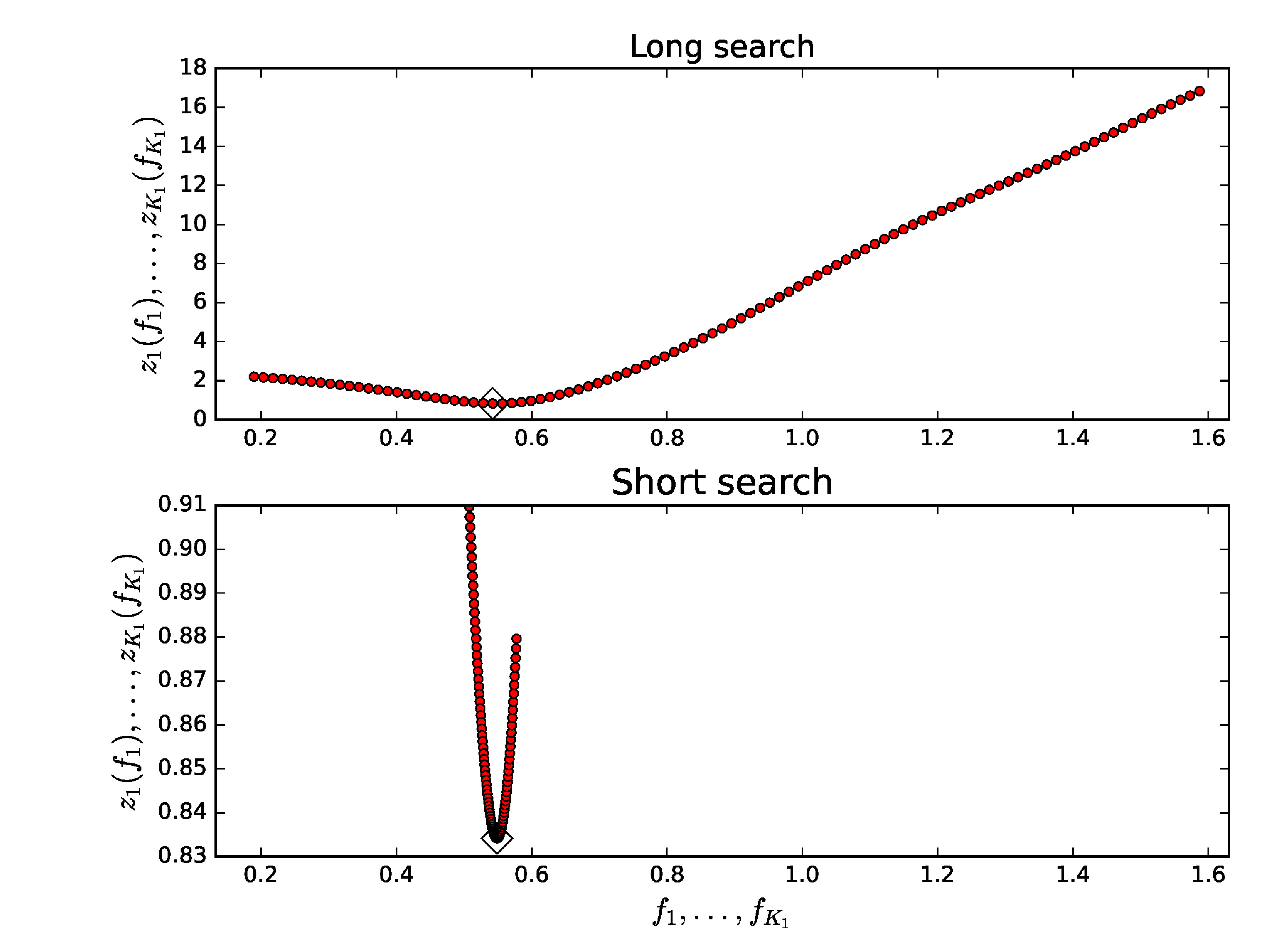
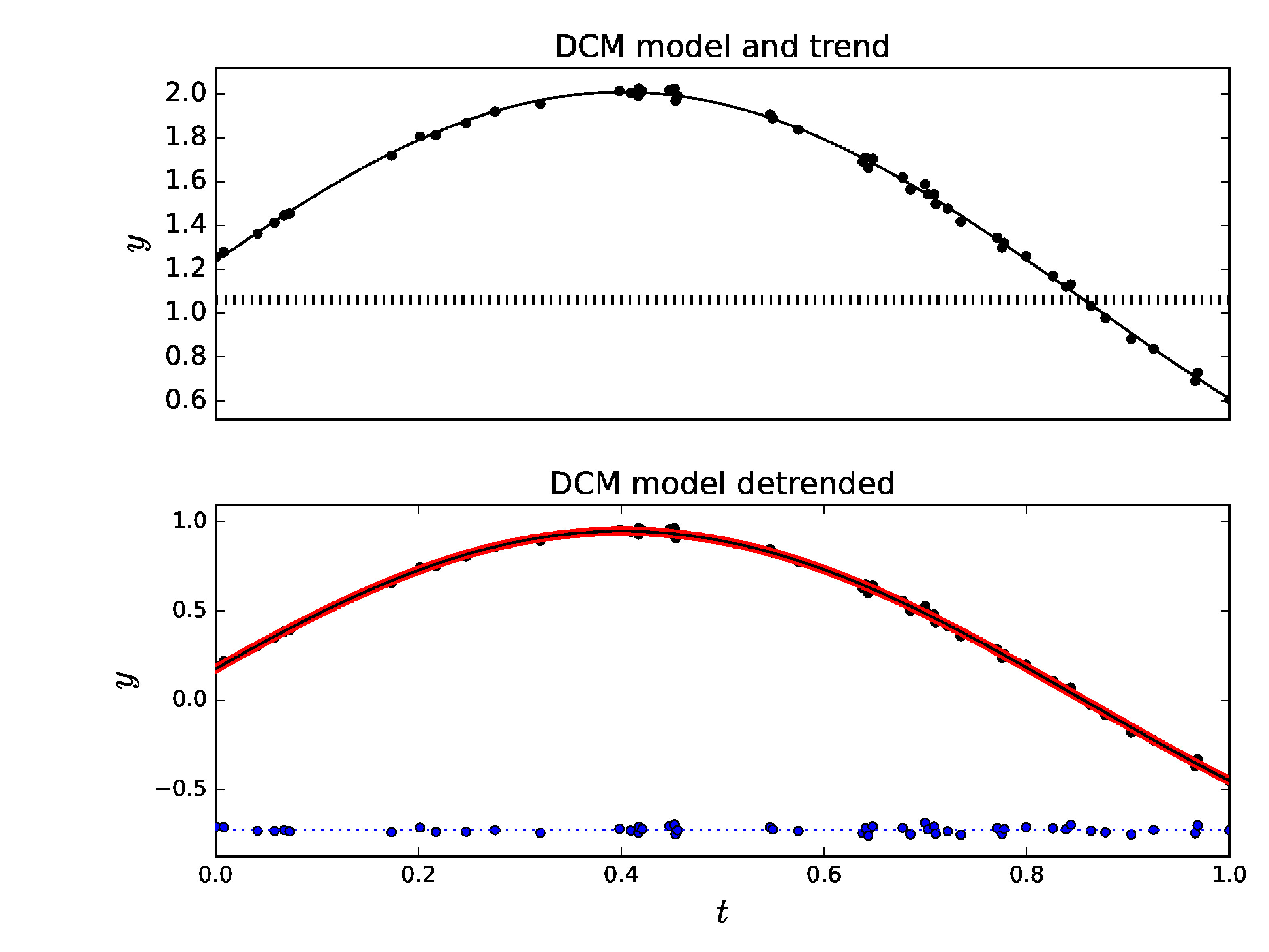
              (a)            (c)

               (b)            (d)

 

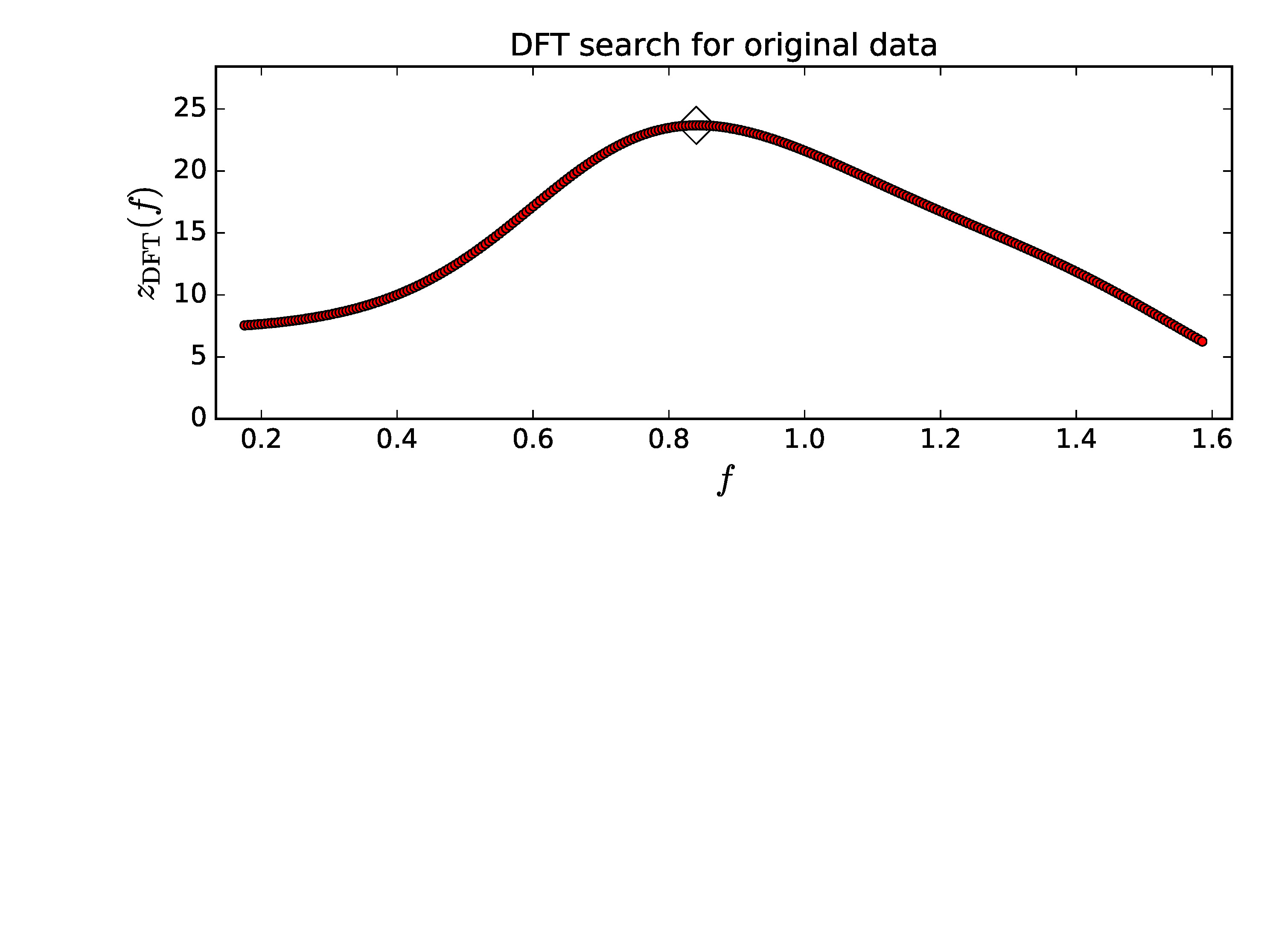
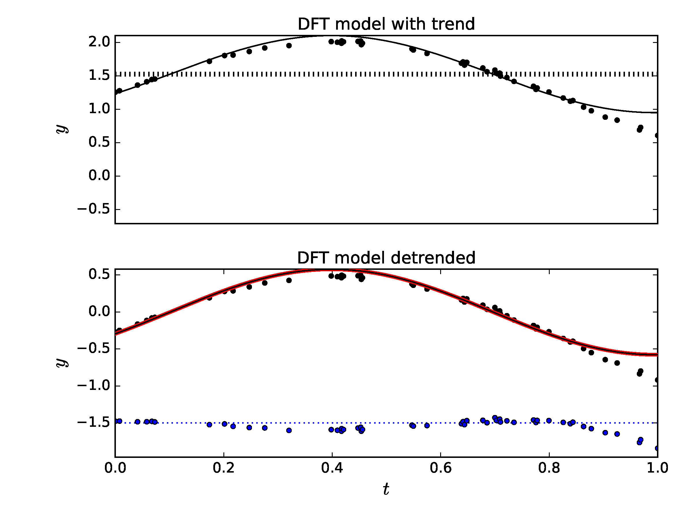
              (e)            (f)

                        (g)

Figure 1: Model 1 (Table 1: $n=50$, ${\mathrm{SN}}=50$ simulation). (a) DCM long search periodogram $z_{1}(f_{1})$ gives best period at 1.843 (diamond). (b) DCM short search periodogram $z_{1}(f_{1})$ gives best period at 1.822 (diamond). (c) DCM model $g(t)$ (black continuous line), DCM trend $p(t)$ (black dashed line) and data $y_{i}$ (black dots). (d) DCM model detrended $g(t)-p(t)$ (black continuous line), DCM signal $h_{1}(t)$ (red thick continuous line), detrended data $y(t_{i})-p(t_{i})$ (black dots) and DCM model residuals $y(t_{i})-g(t_{1})$ (blue dots) offset to -0.65 level (blue dotted line). (e) DFT periodogram $z_{\mathrm{DFT}}(f)$ gives best period at 1.190 (Diamond). (f) DFT model $g_{\mathrm{DFT}}(t)$ (black continuous line), DFT trend $p_{\mathrm{DFT}}(t)$ (black dashed line) and data $y_{i}$ (black dots). (g) DFT model detrended $g_{\mathrm{DFT}}(t)-p_{\mathrm{DFT}}(t)$ (black contiuous line), DFT pure sine $s_{\mathrm{DFT}}(t)$ (red thick continuous line), detrended data $y(t_{i})-p_{\mathrm{DFT}}(t_{i})$ (black dots) and DFT model residuals (blue dots) offset to -1.5 level (blue dotted line).

2.2 Simulated DCM model data samples

We use seven different $g(t)$ models to simulate 21 artificial data samples (Sections 3.1-3.7). The time interval of all simulated samples is $\Delta T=1.$ The $n^{\star}$ simulated time points $t_{i}^{\star}$ are drawn from a random uniform distribution $U(0,\Delta T,n^{\star})$. The first and last time point values are then modified to $t_{1}^{\star}=0$ and $t_{n}^{\star}=\Delta T$. Hence, the distance between independent frequencies [18, 27, 25] is always

$$f_{0}=1/\Delta T=1.$$ (23)

The $n^{\star}$ residuals $\epsilon^{\star}(t_{i}^{\star})$ of simulated model are drawn from a random normal distribution $N(0,\sigma,n^{\star})$, where $\sigma$ is the accuracy of simulated data. The simulated data are

$$y^{\star}(t_{i}^{\star}) = g(t_{i}^{\star})+\epsilon^{\star}(t_{i}^{\star})$$

$$= h(t_{i}^{\star})+p(t_{i}^{\star})+\epsilon^{\star}(t_{i}^{\star}).$$

The peak to peak amplitudes of all simulated signals is $A=2.$ Our definition for the signal to noise ratio is

$${\mathrm{SN}}=(A/2)/\sigma.$$ (24)

2.3 Dicrete Fourier Transform (DFT)

We search for signals in the simulated data using the DFT version formulated by [11]. This method searches for the best pure sine model for the data. The notations for the DFT model are

$$g_{\mathrm{DFT}}(t)=s_{\mathrm{DFT}}(t)+p_{\mathrm{DFT}}(t),$$ (25)

where $s_{\mathrm{DFT}}(t)$ is the pure sine signal and $p_{\mathrm{DFT}}(t)$ is the trend. The pure sine signals for the $y_{i}$ data and the $\epsilon_{i}$ residuals are denoted with $s_{y,\mathrm{DFT}}(t)$ and $s_{\epsilon,\mathrm{DFT}}(t)$, respectively. Our DFT analysis may fail for four main reasons.

The data sample is “too short” [27, 28]

$$P>\Delta T.$$ (26)

The data contain “a trend” [3, 17]

$$p_{\mathrm{DFT}}(t)\neq 0.$$ (27)

The signal frequencies are “too close” [18, 23].

$$|f_{1}-f_{2}|<f_{0}={\Delta T}^{-1}.$$ (28)

The signals are not “pure sines” [16, 2].

$$K_{2}\neq 1.$$ (29)

We search for many pure sine signals using the DFT pre-whitening technique [26, 34]. The $p_{i}=p_{\mathrm{DFT}}(t_{i})$ trend is first removed from the data $y_{i}=y(t_{i})$. In the search for the first signal, we apply the DFT to the detrended $y_{i}-p_{i}$ data. When searching for the second signal, we apply the DTF to the original model residuals $\epsilon_{i}=y_{i}-g_{\mathrm{y,DFT}}(t_{i})$.

3 Results

We apply DCM and DFT to seven different simulated data samples (Sections 3.1 - 3.7). DCM analysis succeeds for all samples. DFT analysis fails for every sample.

3.1 Model 1

Our first simulation model is the one signal model

$$g(t)=(A_{1}/2)\cos{\left[{{2\pi(t-t_{\mathrm{1,max,1}})}\over{P_{1}}}\right]}+M_{0}.$$ (30)

We give the $P_{1}$, $A_{1}$, $t_{\mathrm{1,max,1}}$ and $M_{0}$ values in Table 1 (Column 1). This sample is “too short” (Equation 26) because $P_{1}=1.9\Delta T$. The constant mean level $M_{0}$ is unknown (Equation 27). We perform the DCM and DFT time series analysis between $P_{\mathrm{min}}=P_{1}/3=0.63$ and $P_{\mathrm{max}}=3P_{1}=5.70$.

Model 1 is a DCM model, where $K_{1}=1$, $K_{2}=1$, $K_{3}=0$, $B_{1,1}=$ $(A_{1}/2)\cos{(2\pi f_{1}t_{\mathrm{1,max,1}})}$ and $C_{1,1}=$ $(A_{1}/2)$ $\sin{(2\pi f_{1}t_{\mathrm{1,max,1}})}.$ We give the DCM analysis results for three samples having different $n$ and ${\mathrm{SN}}$ combinations (Table 1: Columns 2-4). For each sample, this table specifies the electronic data file and the electronic DCM control file. The detected $P_{1}$, $A_{1}$, $t_{\mathrm{1,max,1}}$ and $M_{0}$ values are correct and accurate even for the combination $n=50$ and ${\mathrm{SN}}=50$. These values become more accurate when $n$ and ${\mathrm{SN}}$ increase.

A graphical presentation of DCM analysis results is shown for Model 1 simulated data sample, where $n=50$ and ${\mathrm{SN}}=50$ (Figures 1a-d). The DCM long search $z_{1}(f_{1})$ periodogram minimum is at $P_{1}=1.843$ (Figure 1a: diamond). The DCM short search periodogram $z_{1}(f_{1})$ gives the best period at $P_{1}=1.822$ (Figure 1b: diamond). The continuous black line denoting the DCM model $g(t)$ fits perfectly to the black dots denoting the data $y_{i}$ (Figure 1c). The mean $p(t)=M_{0}=1.061\pm 0.036$ is correct (Figure 1c: dashed black line). The detrended model $g(t)-p(t)$ (black continuous line), the detrended data $y(t_{i})-p(t_{i})$ (black dots) and the pure sine signal $h_{1}(t)$ (red thick continuous line) are shown in Figure 1d. Note that the thick continuous red line stays under the thin continuous black line because $h_{1}(t)=g(t)-p(t)$. The DCM residuals (blue dots) are offset to the level of -0.65 (blue dotted line). These residuals are stable and display no trends.

The DFT detects the wrong period $P_{1}=1.190$ (Figure 1e: Diamond). The DFT mean level estimate $M_{0}=1.527$ is also wrong (Figure 1f: Dashed black line). The black dots denoting the data $y_{i}$ deviate from the continuous black line denoting the DFT model $g_{\mathrm{DFT}}(t)$. The detrended model $g_{\mathrm{DFT}}(t)-p_{\mathrm{DFT}}(t)$ (continuous black line), the detrended data $y(t_{i})-p_{\mathrm{DFT}}(t_{i})$ (black dots) and the signal $s_{\mathrm{y,DFT}}(t)$ (continuous thick red line) are shown in Figure 1g. The thin black line covers the thick red line because $s_{\mathrm{y,DFT}}(t)=g_{\mathrm{DFT}}(t)-p_{\mathrm{DFT}}(t)$. The DFT residuals (blue dots) offset to the level of -1.5 (blue dotted line) display obvious trends, especially at the end of analysed sample.

For the simulated data of Model 1, the DCM analysis succeeds, but the DFT analysis fails.

Table 2: Model 2. DCM analysis between $P_{\mathrm{min}}=0.63$ and $P_{\mathrm{max}}=4.70$. Notations as in Table 1.

(1)	(2)	(3)	(4)
	$n=1~000$	$n=10~000$	$n=10~000$
Model 2	${\mathrm{SN}}=100$	${\mathrm{SN}}=100$	${\mathrm{SN}}=200$
$P_{1}=1.9$	$1.98\pm 0.34$	$1.852\pm 0.055$	$1.933\pm 0.040$
$A_{1}=2.0$	$2.4\pm 2.8$	$1.84\pm 0.20$	$2.13\pm 0.16$
$t_{\mathrm{1,min,1}}=1.35$	$1.39\pm 0.17$	$1.326\pm 0.027$	$1.367\pm 0.020$
$t_{\mathrm{1,max,1}}=0.40$	$0.4015\pm 0.0020$	$0.40007\pm 0.00072$	$0.40017\pm 0.00075$
$M_{0}=1.0$	$0.8\pm 1.4$	$1.079\pm 0.096$	$0.937\pm 0.080$
$M_{1}=0.25$	$0.29\pm 0.21$	$0.229\pm 0.026$	$0.266\pm 0.020$
$M_{2}=0.50$	$0.62\pm 0.52$	$0.451\pm 0.064$	$0.540\pm 0.049$
Data file	Model2n1000SN100.dat	Model2n10000SN100.dat	Model2n10000SN200.dat
Control file	dcmModel2n1000SN100.dat	dcmModel2n10000SN100.dat	dcmModel2n10000SN200.dat

 

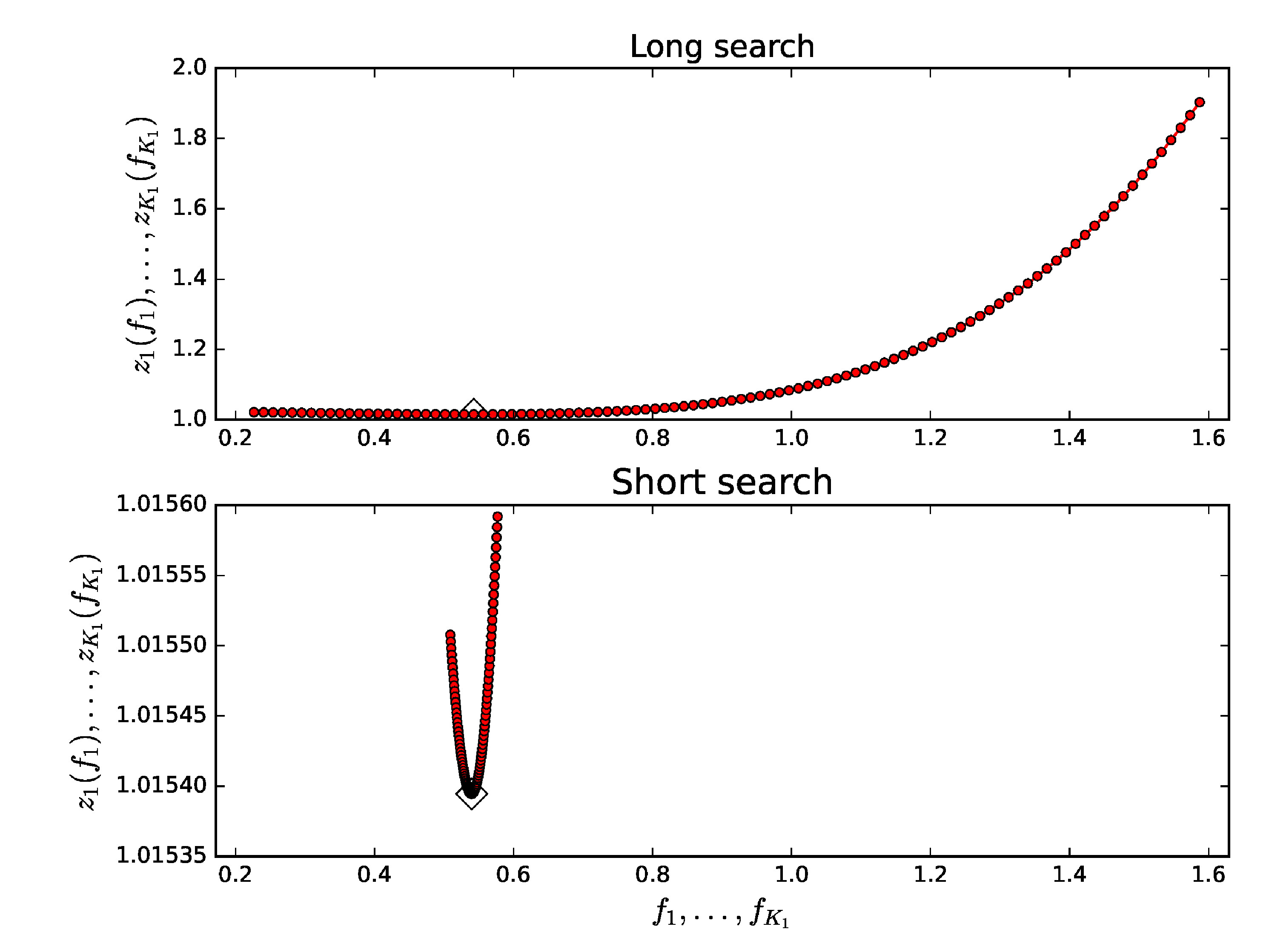
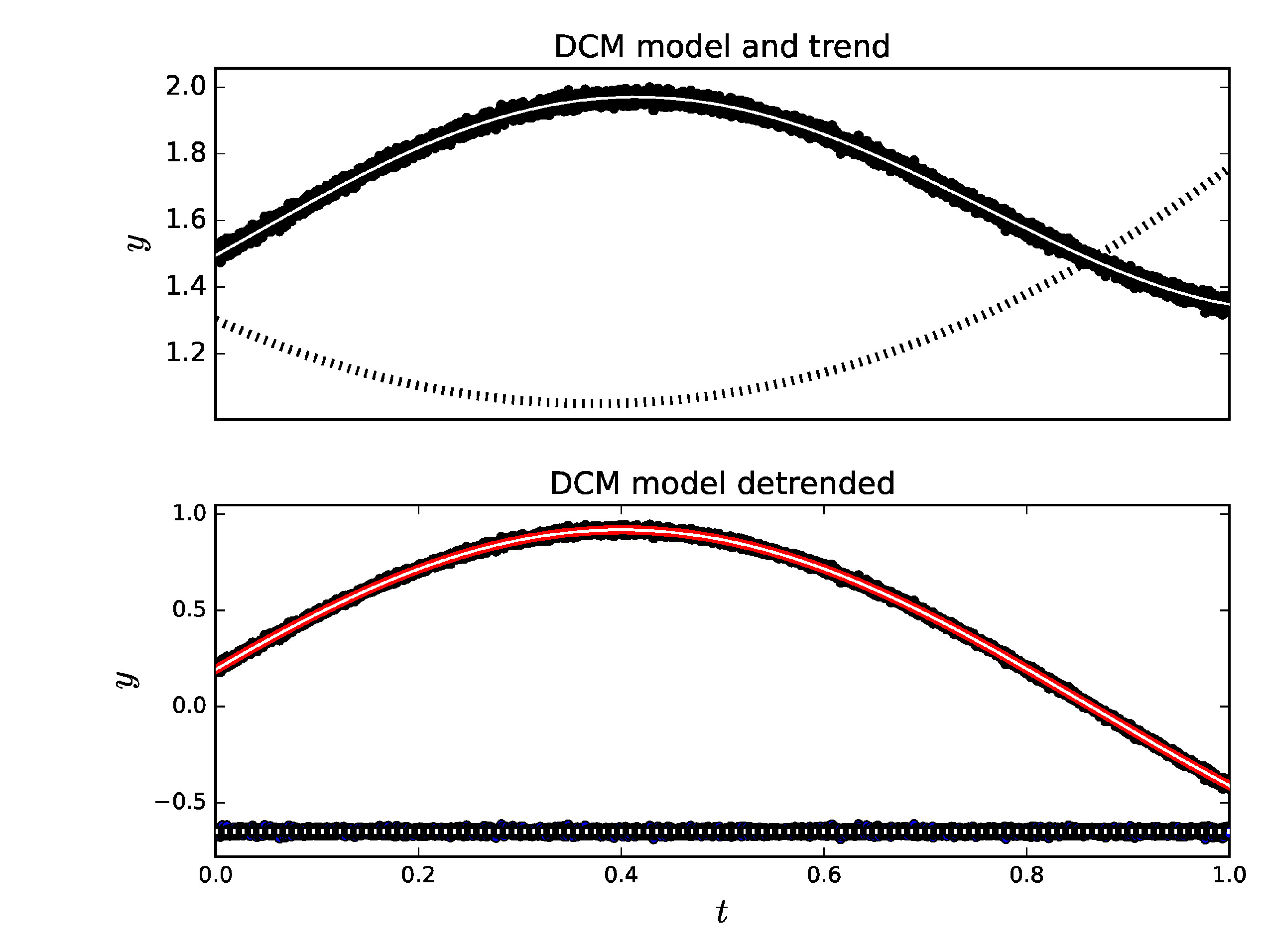
              (a)            (c)

              (b)            (d)

 

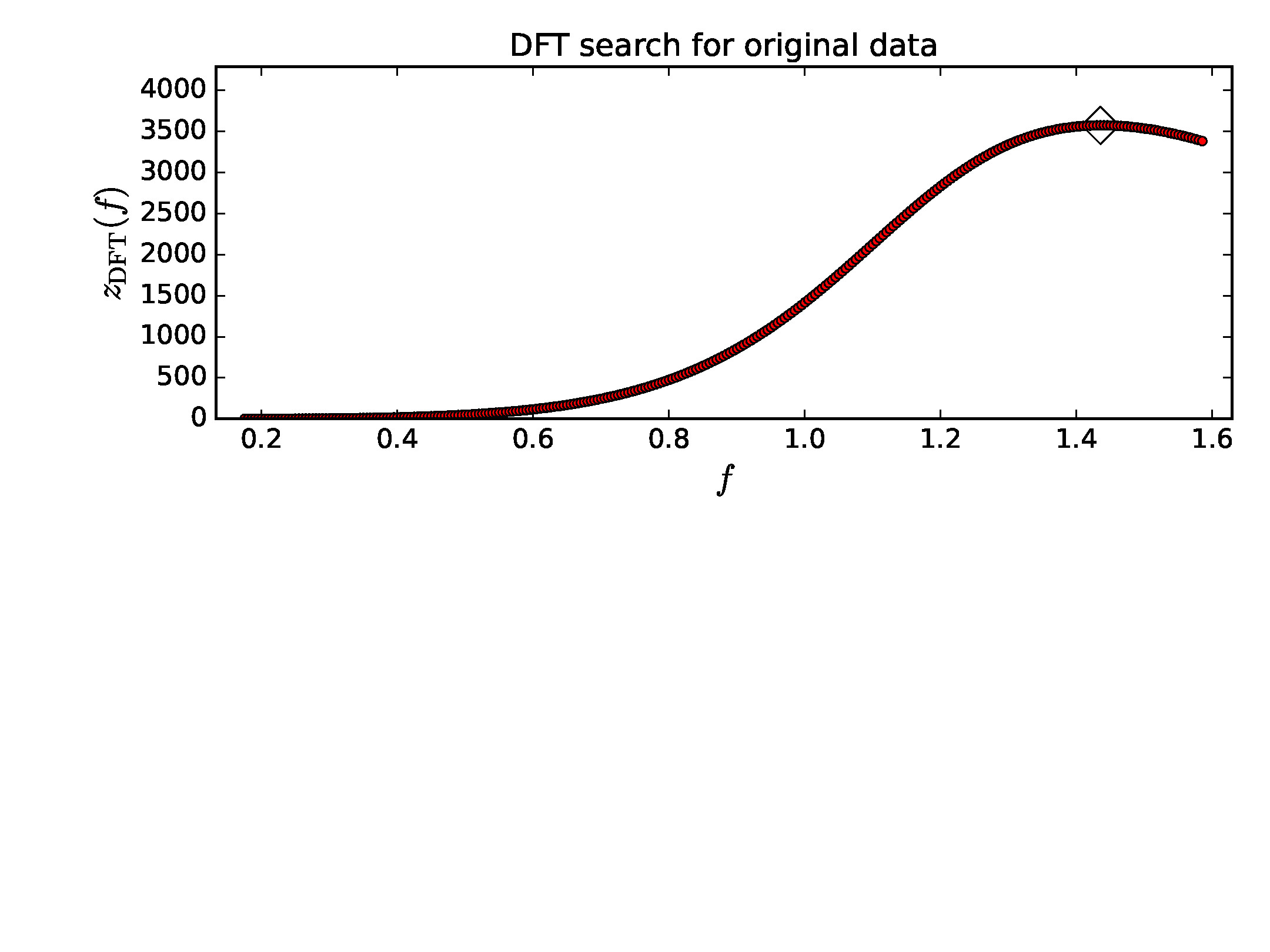
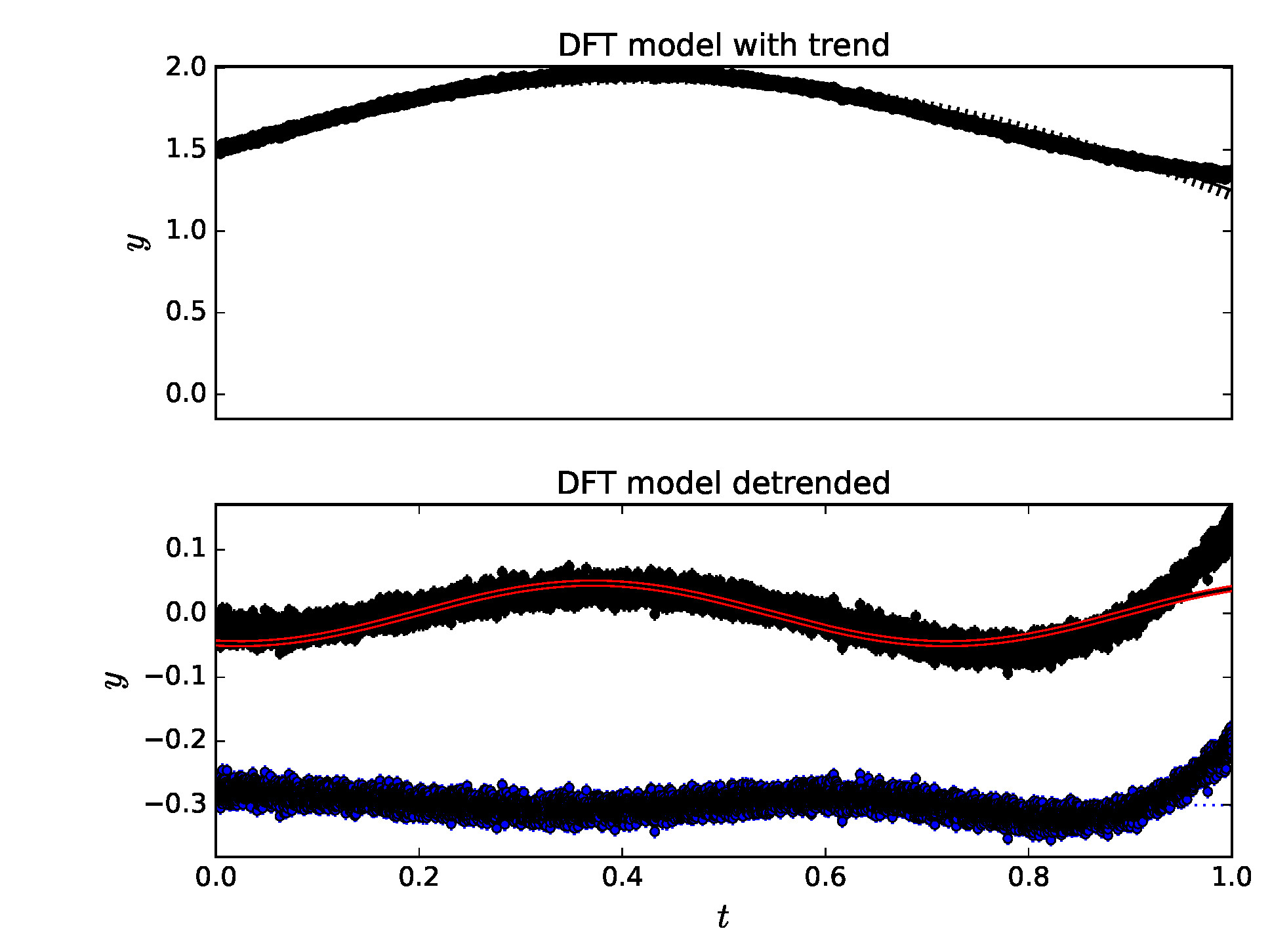
              (e)            (f)

                        (g)

Figure 2: Model 2 (Table 2: $n=10~000$, ${\mathrm{SN}}=100$ simulation). (c) Colour of $g(t)$ line has been changed from black to white. (d) Colour of $g(t)$ line has been changed from black to white. Colour of offset level -0.3 dotted line has been changed from blue to white. Locations of best periods (diamonds) are explained in text (Section 3.2). Otherwise, notations are as in Figure 1.

Table 3: Model 3. DCM analysis between $P_{\mathrm{min}}=0.053$ and $P_{\mathrm{max}}=0.480$. Notations as in Table 1.

(1)	(2)	(3)	(4)
	$n=50$	$n=50$	$n=100$
Model 3	${\mathrm{SN}}=10$	${\mathrm{SN}}=50$	${\mathrm{SN}}=100$
$P_{1}=0.16$	$0.15898\pm 0.00068$	$0.15989\pm 0.00014$	$0.159950\pm 0.000077$
$A_{1}=2.0$	$1.85\pm 0.10$	$1.987\pm 0.036$	$1.994\pm 0.015$
$t_{\mathrm{1,min,1}}=0.11$	$0.1122\pm 0.0020$	$0.11080\pm 0.00088$	$0.11004\pm 0.00030$
$t_{\mathrm{1,max,1}}=0.03$	$0.0328\pm 0.0022$	$0.03086\pm 0.00094$	$0.03007\pm 0.00033$
$P_{2}=0.17$	$0.17025\pm 0.00066$	$0.17018\pm 0.00024$	$0.16996\pm 0.00080$
$A_{2}=2.0$	$2.001\pm 0.090$	$1.962\pm 0.046$	$2.002\pm 0.012$
$t_{\mathrm{2,min,1}}=0.135$	$0.1312\pm 0.0022$	$0.13461\pm 0.00087$	$0.13495\pm 0.00031$
$t_{\mathrm{2,max,1}}=0.05$	$0.0461\pm 0.0024$	$0.04952\pm 0.00099$	$0.04997\pm 0.000038$
$M_{0}=1.0$	$0.996\pm 0.011$	$0.9985\pm 0.0032$	$0.9995\pm 0.0012$
Data file	Model3n50SN10.dat	Model3n50SN50.dat	Model3n100SN100.dat
Control file	dcmModel3n50SN10.dat	dcmModel3n50SN50.dat	dcmModel3n100SN100.dat

 

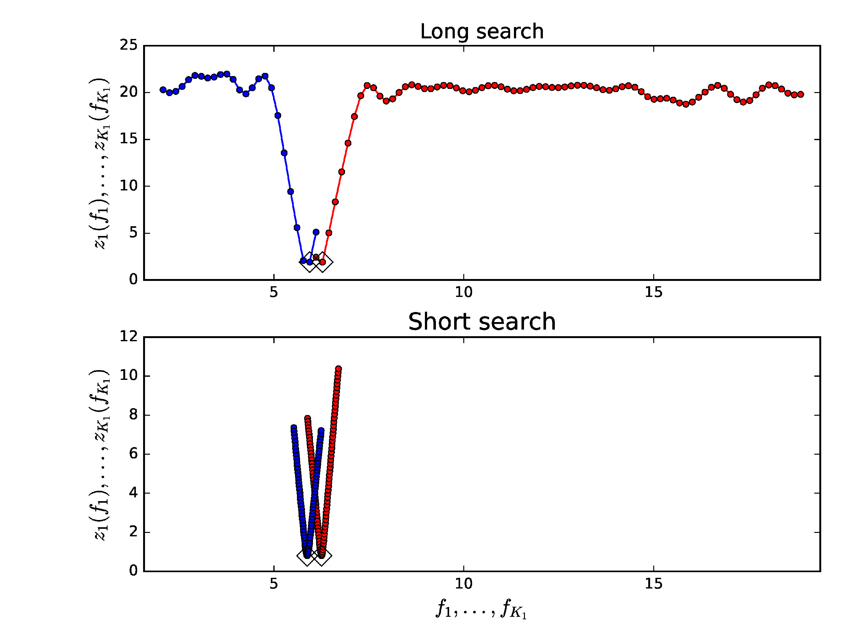
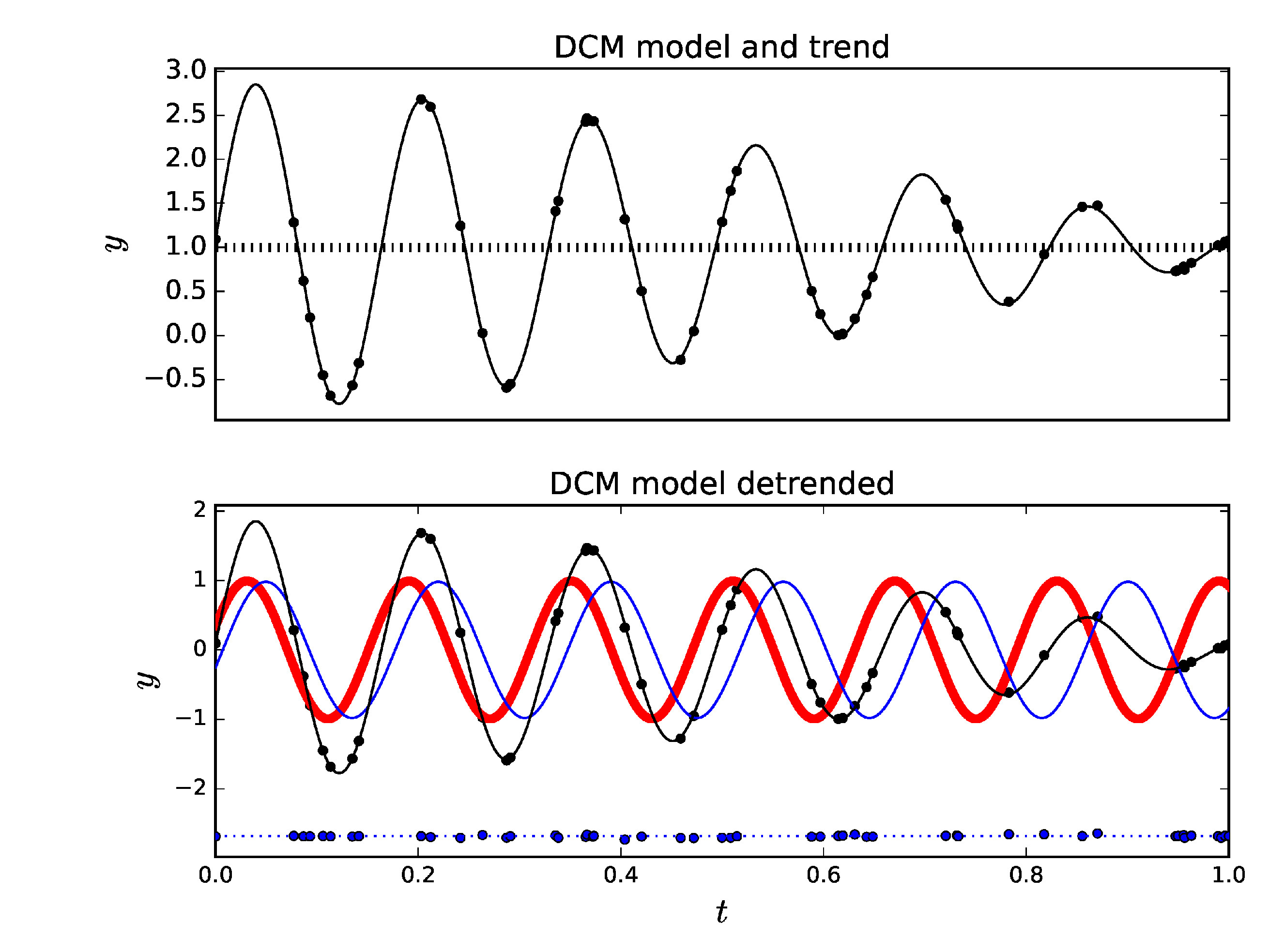
               (a)            (c)

               (b)            (d)

 

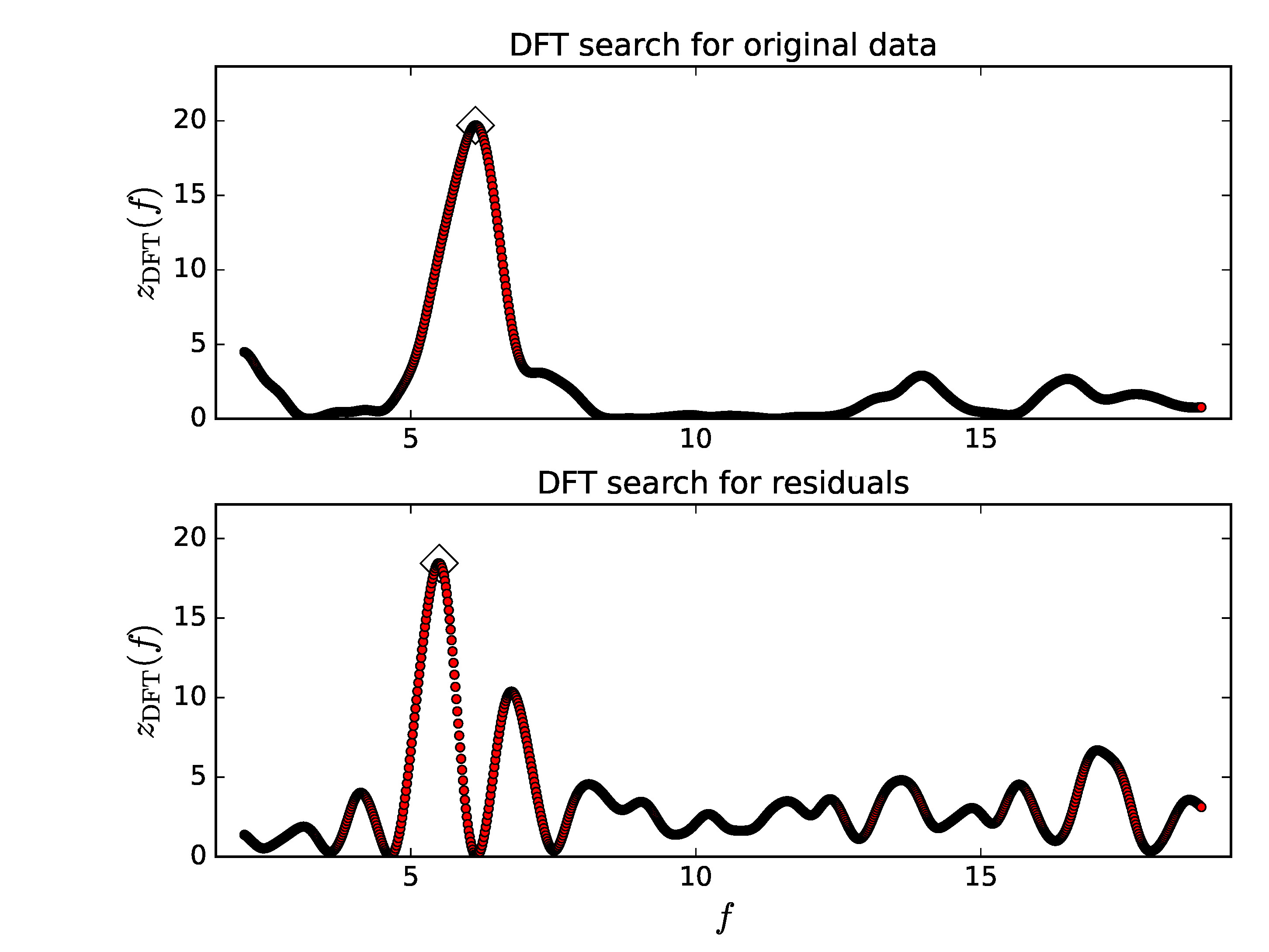
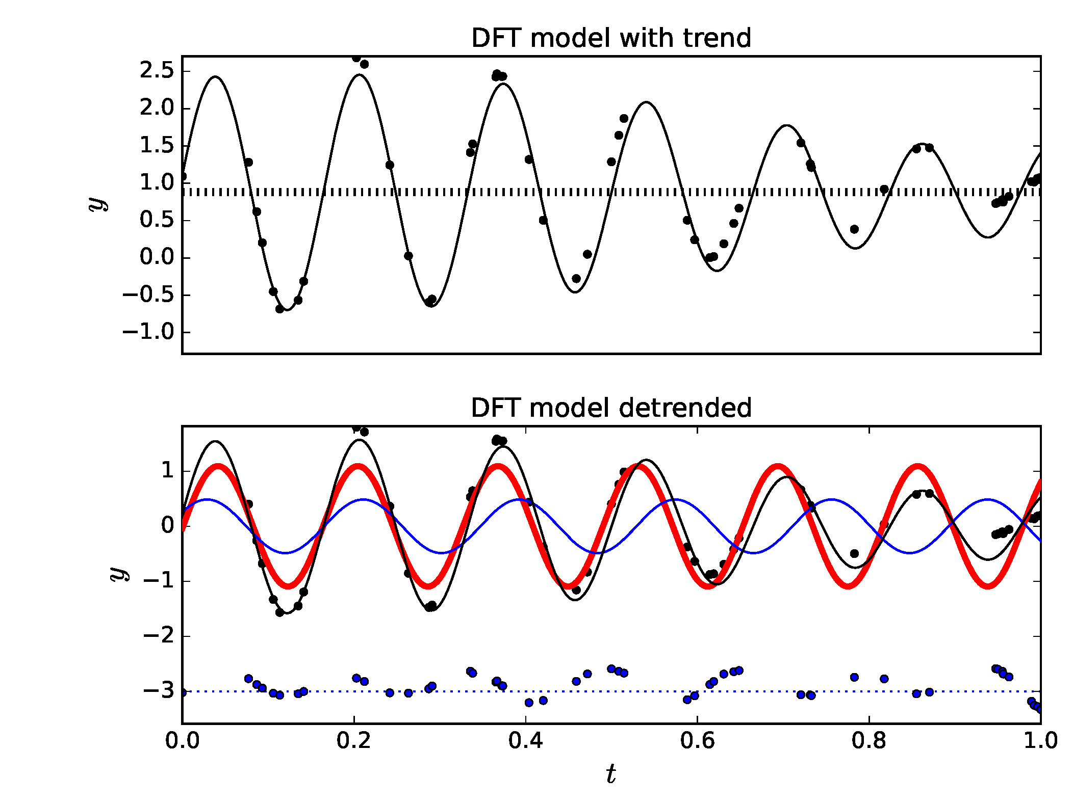
               (e)            (g)

              (f)             (h)

Figure 3: Model 3 (Table 3: $n=50$, ${\mathrm{SN}}=50$ simulation). (a) DCM long search periodograms $z_{1}(f_{1})$ (red) and $z_{2}(f)$ (blue) give best periods at 0.160 and 0.168 (diamonds). (b) DCM short search periodograms $z_{1}(f_{1})$ (red) and $z_{2}(f)$ (blue) give best periods at 0.160 and 0.170 (diamonds). (c) DCM model $g(t)$ (black continuous line), DCM trend $p(t)$ (black dashed line) and data $y_{i}$ (black dots). (d) DCM model detrended $g(t)-p(t)$ (black continuous line), DCM signal $h_{1}(t)$ (red thick continuous line), DCM signal $h_{2}(t)$ (blue continuous thin line), detrended data $y(t_{i})-p(t_{i})$ (black dots) and DCM model residuals $y(t_{i})-g(t_{1})$ (blue dots) offset to -3.0 level (blue dotted line) (e) DFT periodogram $z_{\mathrm{DFT}}(f)$ for the original data gives best period at 0.163 (diamond). (f) DFT periodogram $z_{\mathrm{DFT}}(f)$ for the sine model residuals gives best period at 0.182 (diamond). (g) DFT model $g_{\mathrm{DFT}}(t)$ (black continuous line), DFT trend $p_{\mathrm{DFT}}(t)$ (black dashed line) and data $y_{i}$ (black dots). (h) DFT model detrended $g_{\mathrm{DFT}}(t)-p_{\mathrm{DFT}}(t)$ (black continuous line), DFT pure sine model for original data $s_{y,\mathrm{DFT}}(t)$ (red thick continuous line), DFT pure sine model for first residuals $s_{\epsilon,\mathrm{DFT}}(t)$ (blue continuous thin line), detrended data $y(t_{i})-p_{\mathrm{DFT}}(t_{i})$ (black dots) and DFT model residuals (blue dots) offset to -3.0 level (blue dotted line).

Table 4: Model 4. DCM analysis between $P_{\mathrm{min}}=0.053$ and $P_{\mathrm{max}}=0.480$. Notations as in Table 1.

(1)	(2)	(3)	(4)
	$n=50$	$n=50$	$n=100$
Model 4	${\mathrm{SN}}=10$	${\mathrm{SN}}=50$	${\mathrm{SN}}=100$
$P_{1}=0.16$	$0.1606\pm 0.0084$	$0.15982\pm 0.00023$	$0.16001\pm 0.000058$
$A_{1}=2.0$	$1.97\pm 0.15$	$1.958\pm 0.051$	$2.012\pm 0.014$
$t_{\mathrm{1,min,1}}=0.11$	$0.1134\pm 0.0036$	$0.11059\pm 0.00088$	$0.10977\pm 0.00033$
$t_{\mathrm{1,max,1}}=0.03$	$0.0331\pm 0.0040$	$0.03068\pm 0.00097$	$0.02976\pm 0.00035$
$P_{2}=0.17$	$0.1744\pm 0.0012$	$0.17009\pm 0.00026$	$0.169958\pm 0.000092$
$A_{2}=2.0$	$1.74\pm 0.17$	$1.982\pm 0.044$	$2.018\pm 0.017$
$t_{\mathrm{2,min,1}}=0.135$	$0.1321\pm 0.0044$	$0.1342\pm 0.0011$	$0.13528\pm 0.00042$
$t_{\mathrm{2,max,1}}=0.05$	$0.0460\pm 0.0048$	$0.0492\pm 0.0012$	$0.05031\pm 0.00034$
$M_{0}=1.0$	$1.015\pm 0.024$	$0.9997\pm 0.0030$	$1.0012\pm 0.0016$
$M_{1}=0.25$	$0.219\pm 0.023$	$0.2565\pm 0.0066$	$0.2495\pm 0.0019$
$M_{2}=0.5$	$0.485\pm 0.050$	$0.511\pm 0.011$	$0.4983\pm 0.0033$
Data file	Model4n50SN10.dat	Model4n50SN50.dat	Model4n100SN100.dat
Control file	dcmModel4n50SN10.dat	dcmModel4n50SN50.dat	dcmModel4n100SN100.dat

 

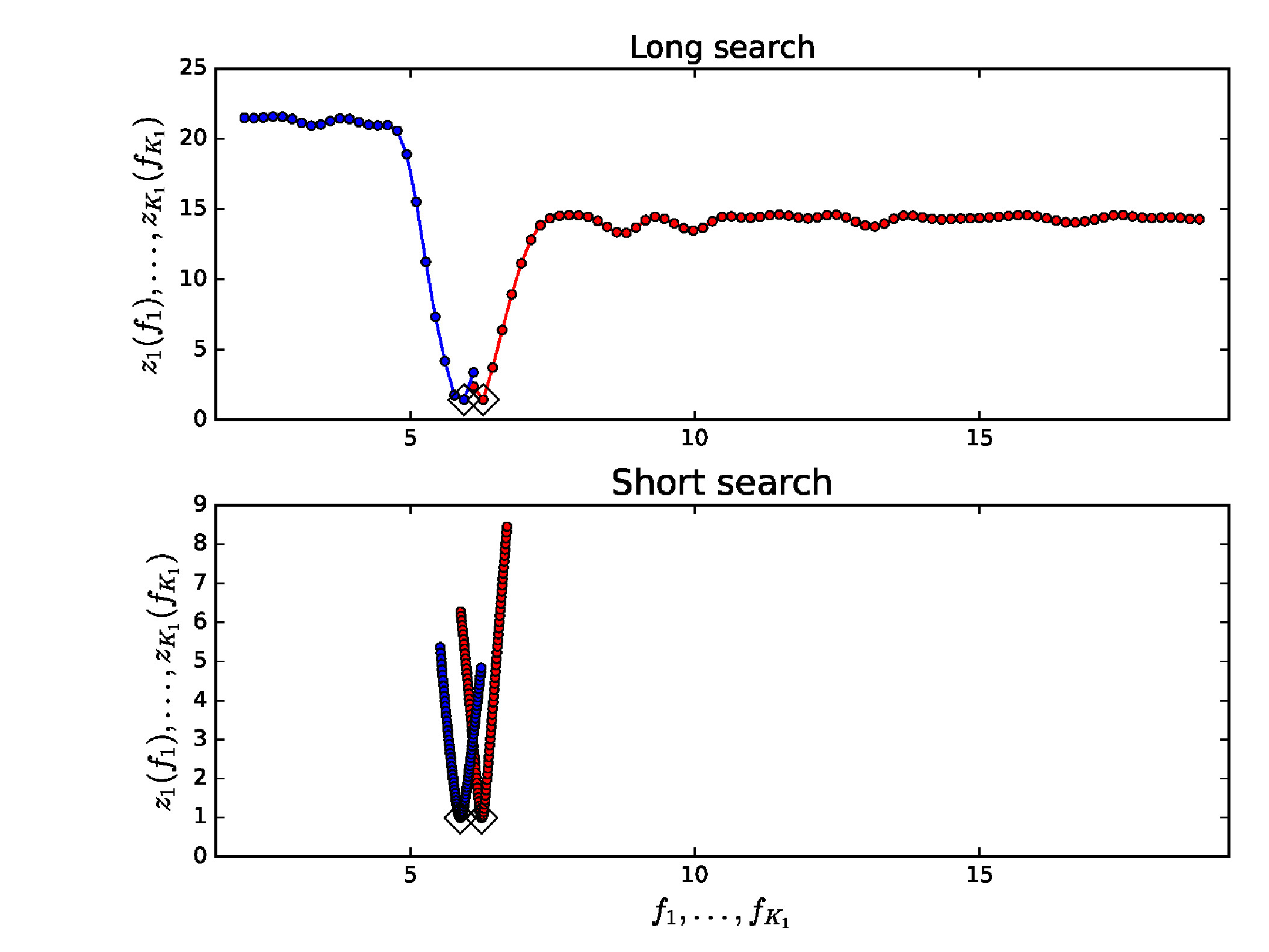
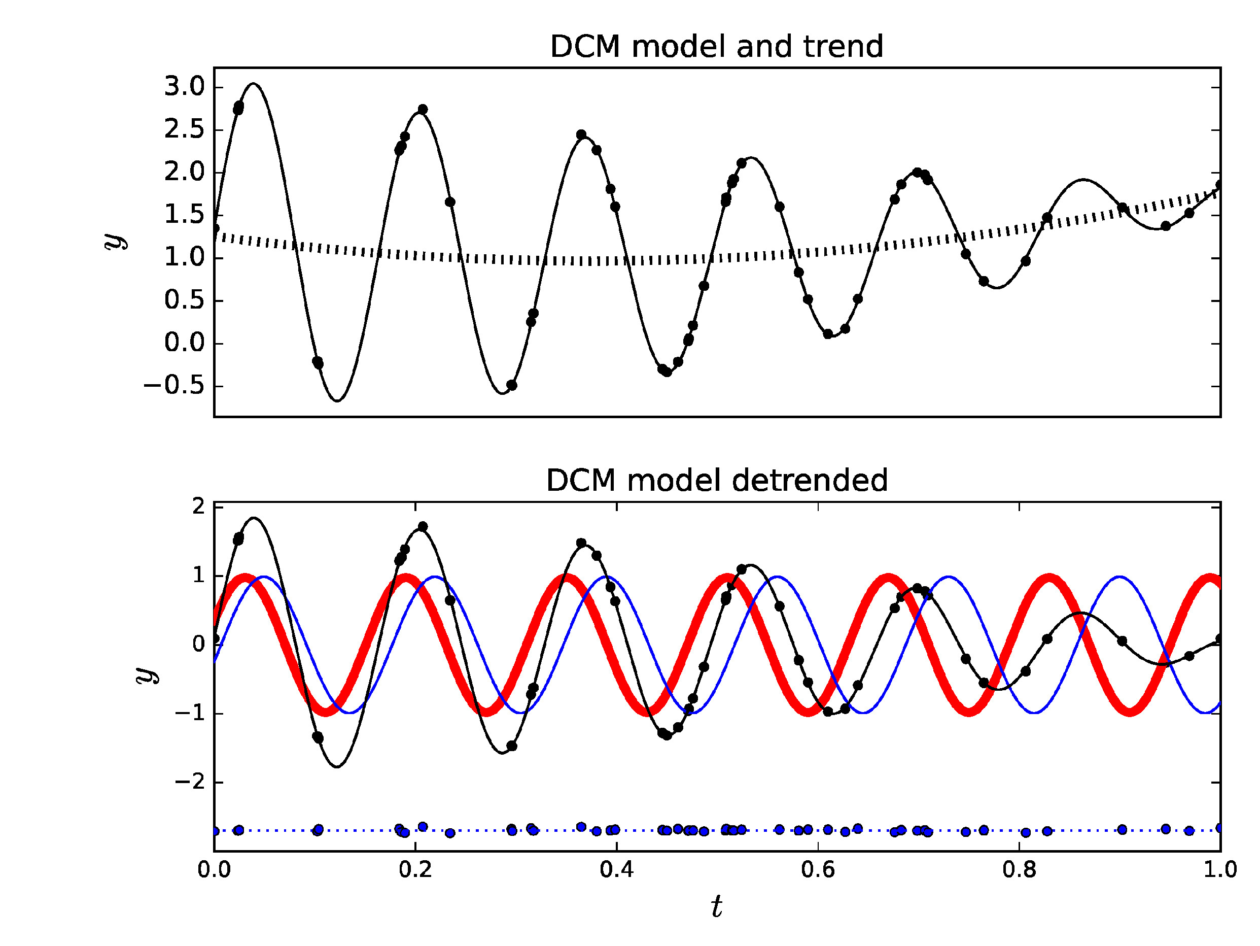
              (a)            (c)

              (b)            (d)

 

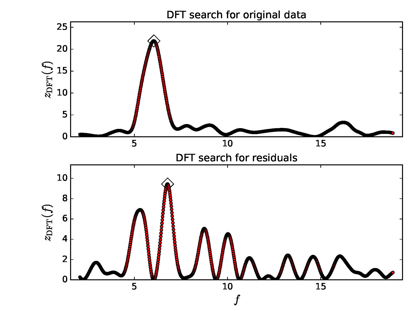
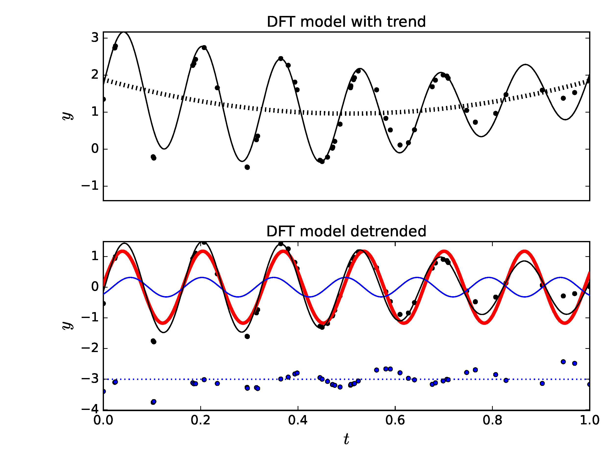
              (e)             (g)

              (f)             (h)

Figure 4: Model 4 (Table 4: $n=50$, ${\mathrm{SN}}=50$ simulation). Notations as in Figure 3. Best periods (diamonds) are explained in Section 3.4.

3.2 Model 2

Our next one signal data simulation model is

$$g(t) = (A_{1}/2)\cos{\left[{{2\pi(t-t_{\mathrm{1,max,1}})}\over{P_{1}}}\right]}$$

$$+ M_{0}+M_{1}T+M_{2}T^{2}$$

where $T=[2(t-t_{\mathrm{mid}})]/\Delta T$. We give the $P_{1}$, $A_{1}$, $t_{\mathrm{1,max,1}}$, $M_{0}$, $M_{1}$ and $M_{2}$ values in Table 2. As a DCM model, the orders of Model 2 are $K_{1}=1$, $K_{2}=1$ and $K_{3}=2$. The simulated data sample is “too short” because the period $P_{1}$ is $1.9\times\Delta T$ (Equation 26). The parabolic trend $p(t)$ is unknown (Equation 27). Again, we use the DCM and DFT time series analysis methods to search for periods between $P_{\mathrm{min}}=P_{1}/3=0.63$ and $P_{\mathrm{max}}=3P_{1}=4.70$.

The DCM analysis results are given in Table 2. These results are not very accurate for the $n=100$ and ${\mathrm{SN}}=100$ combination, but they definitely improve for larger $n$ and ${\mathrm{SN}}$ values. For Model 2, the DCM analysis results are illustrated for the $n=10~000$ and ${\mathrm{SN}}=100$ combination (Figures 2a-d). The DCM long search $z_{1}(f_{1})$ periodogram minimum is at $P_{1}=1.843$ (Figure 2a: diamond). The DCM short search gives the value $P_{1}=1.852$ (Figure 2b: diamond). The DCM model $g(t)$ is so good that it’s continuous black line is totally covered by the black dots representing the $y_{i}$ data (Figure 2c). Therefore, the colour of this $g(t)$ line has been changed from black to white. The results for the parabolic trend coefficients $M_{0}=1.079\pm 0.096$, $M_{1}=0.229\pm 0.026$ and $M_{2}=0.451\pm 0,064$ of the dashed black $p(t)$ line are correct. In Figure 1d, the white continuous line shows the detrended model $g(t)-p(t)$. The black dots show the detrended data $y(t_{i})-p(t_{i})$ and the red thick continuous line shows the pure sine signal $h_{1}(t)$. Note that the red thick line is under the white thin line because $h_{1}(t)=g(t)-p(t)$. The DCM residuals (blue dots) are offset to the level of -0.65. The colour of dotted line, which denotes this offset level, has been changed from blue to white. The distribution of these DCM model residuals is stable, as expected for a random normal distribution.

The wrong period $P_{1}=0.697$ is detected by DFT (Figure 2e: Diamond). The DFT estimates for the trend $p(t)$ coefficients, $M_{0}=1.92$, $M_{1}=-0.15$ and $M_{2}=-0.56$ are also wrong (Figure 2f: dashed black line). The data $y_{i}$ (black dots) deviate from the DFT model $g_{\mathrm{DFT}}(t)$ (black continuous line), especially in the end of the sample (Figure 2g). For the detrended DFT model, the thin black line covers the thick red line because $s_{\mathrm{y,DFT}}(t)=g_{\mathrm{DFT}}(t)-p_{\mathrm{DFT}}(t)$ (Figure 2g). The $s_{\mathrm{y,DFT}}(t)$ sine curve peak to peak amplitude is far below the correct $A_{1}=2.0$ value. The DFT residuals (blue dots) are offset to the level of -1.5 (blue dotted line). The trends of these residuals confirm that the DFT analysis fails.

Only DCM (not DFT) succeeds in the analysis of Model 2 simulated data.

3.3 Model 3

Our third data simulation model is the two signal model

$$g(t) = (A_{1}/2)\cos{\left[{{2\pi(t-t_{\mathrm{1,max,1}})}\over{P_{1}}}\right]}$$

$$+ (A_{2}/2)\cos{\left[{{2\pi(t-t_{\mathrm{2,max,1}})}\over{P_{2}}}\right]}+M_{0}.$$

We give the $P_{1}$, $P_{2}$, $A_{1}$,$A_{2}$, $t_{\mathrm{1,max,1}}$, $t_{\mathrm{2,max,1}}$ and $M_{0}$ values in Table 3 (Column 1). The DCM orders of Model 3 are $K_{1}=2$, $K_{2}=1$ and $K_{3}=0$. The simulated data sample is not “too short” (Equation 26) because $P_{1}<P_{2}<\Delta T$. The $p(t)$ trend mean level $M_{0}$ is unknown (Equation 27). The two frequencies are “too close” because $\Delta f=f_{1}-f_{2}=f_{0}/2.72$ (Equation 28). We apply the DCM and DFT time series analyses to search for periods between $P_{\mathrm{min}}=P_{1}/3=0.053$ and $P_{\mathrm{max}}=3P_{1}=0.480$.

The DCM analysis results for different $n$ and ${\mathrm{SN}}$ combinations are given in Table 3 (Columns 2-4). The results are surprisingly accurate even for the small $n=50$ sample having a low ${\mathrm{SN}}=10$. The DCM results for Model 3 are illustrated in Figures 1a-d ($n=50$ and ${\mathrm{SN}}=50$ combination). The DCM long search $z_{1}(f_{1})$ periodogram (red) and $z_{2}(f)$ periodogram (blue) minima are at the best periods $P_{1}=0.159$ and $P_{2}=0.168$ (Figure 3a: diamonds). The DCM short search gives $P_{1}=0.160$ and $P_{2}=0.170$ (Figure 3b: diamonds). The black continuous DCM model $g(t)$ curve crosses trough the black dots of $y_{i}$ data (Figure 1c). The result $M_{0}=0.9985\pm 0.0032$ for the dashed black $p(t)$ trend line is correct. Our Figure 3d shows the detrended DCM model $g(t)-p(t)$ (black continuous line), the detrended data $y(t_{i})-p(t_{i})$ (black dots), the pure sine signal $h_{1}(t)$ (red thick continuous line) and the pure sine signal $h_{2}(t)$ (blue thin continuous line). The DCM residuals (blue dots) are offset to the level of -3.0 (blue dotted line). These residuals are small and their level is stable.

The DFT detects the wrong period $P_{1}=1.163$ for the original data (Figure 3e: diamond). This is an expected result because the detected period should be close to $(P_{1}+P_{2})/2$ when the peak to peak amplitudes of the simulated data, $A_{1}=A_{2}$, are equal (Jetsu 2025). The two DFT periodogram $z_{\mathrm{DFT}}(f)$ peaks at frequencies $1/P_{1}$ and $1/P_{2}$ overlap and merge into one peak. The period $P_{2}=0.182$ detected for the residuals is also wrong (Figure 3f: diamond). The DFT trend $p_{\mathrm{PDF}}(t)$ estimate $M_{0}=0.880$ fails (Figure 3f: dashed black line). The black dots $y_{i}$ show minor deviations from the continuous black DFT model $g_{\mathrm{DFT}}(t)$ line (Figure 3g). The detrended model $g_{\mathrm{DFT}}(t)-p_{\mathrm{DFT}}(t)$ (continuous black line), the detrended data $y(t_{i})-p_{\mathrm{DFT}}(t_{i})$ (black dots), the pure sine signal $s_{\mathrm{y,DFT}}(t)$ for the data (continuous thick red line) and the pure sine signal $s_{\mathrm{\epsilon,DFT}}(t)$ for the residuals (continuous blue thin line) are shown in Figure 3h. Note that the $s_{\mathrm{y,DFT}}(t)$ and $s_{\mathrm{\epsilon,DFT}}(t)$ signal amplitudes are far from equal. The DFT residuals (blue dots) offset to the level of -3.0 (blue dotted line) are not stable.

The DCM analysis of Model 3 simulated data succeeds, but the DFT analysis does not.

3.4 Model 4

The next data simulation model is

$$g(t) = (A_{1}/2)\cos{\left[{{2\pi(t-t_{\mathrm{1,max,1}})}\over{P_{1}}}\right]}$$

$$+ (A_{2}/2)\cos{\left[{{2\pi(t-t_{\mathrm{2,max,1}})}\over{P_{2}}}\right]}$$

$$+ M_{0}+M_{1}T+M_{2}T^{2},$$

where $T=[2(t-t_{\mathrm{mid}})]/\Delta T$. In this model, two signals are superimposed on an unknown parabolic trend. The $P_{1}$, $P_{2}$, $A_{1}$,$A_{2}$, $t_{\mathrm{1,max,1}}$, $t_{\mathrm{2,max,1}}$, $M_{0}$, $M_{1}$ and $M_{2}$ values are given in Table 4. This simulated sample is not “too short” (Equation 26). The polynomial trend $p(t)$ is unknown (Equation 27). The $\Delta f=f_{1}-f_{2}=f_{0}/2.72$ difference means that the frequencies are “too close” (Equation 28). The DCM and DFT time series analysis methods are used to search for periods between $P_{\mathrm{min}}=P_{1}/3=0.053$ and $P_{\mathrm{max}}=3P_{1}=0.480$.

Model 4 is a DCM model having orders $K_{1}=2$, $K_{2}=1$ and $K_{3}=2$. Our DCM analysis results for different $n$ and ${\mathrm{SN}}$ combinations are given in Table 4 (Columns 2-4). The DCM detects the correct $P_{1}$, $P_{2}$, $A_{1}$, $A_{2}$, $t_{\mathrm{max,1}}$, $t_{\mathrm{max,2}}$, $M_{0}$, $M_{1}$ and $M_{2}$ values even for the lowest $n=50$ and ${\mathrm{SN}}=10$ combination. Our Figures 4a-d illustrate the DCM analysis results for one sample of simulated data (Model 4: $n=50$ and ${\mathrm{SN}}=50$). The DCM long search best periods are at $P_{1}=0.159$ and $P_{2}=0.168$ (Figure 4a: diamonds). The DCM short search values are $P_{1}=0.160$ and $P_{2}=0.170$ (Figure 4b: diamonds). The continuous DCM model $g(t)$ black line crosses through all black dots representing the $y_{i}$ data (Figure 4c). The DCM detects the correct polynomial trend $p(t)$ coefficients $M_{0}=0.9997\pm 0.0030$, $M_{1}=0.2565\pm 0.0066$ and $M_{2}=0.511\pm 0.011$ (Figure 4c: dashed black line). The detrended DCM model $g(t)-p(t)$ (black continuous line), the detrended data $y(t_{i})-p(t_{i})$ (black dots), the pure sine signal $h_{1}(t)$ (red thick continuous line) and the pure sine signal $h_{2}(t)$ (blue thin continuous line) are shown in Figure 4d. The DCM residuals (blue dots) offset to the level of -3.0 show no trends and are extremely stable.

Since the peak to peak amplitudes of the simulated data signals are equal, $A_{1}=A_{2}$, the expected result for the DFT analysis of original data is $(P_{1}+P_{2})/2$, where $P_{1}$ and $P_{2}$ are the simulated signal periods (Jetsu 2025). The DFT detects this expected wrong period $P_{1}=1.165$ for the original data (Figure 4e: diamond). A wrong period $P_{2}=0.147$ is also detected for the residuals (Figure 4f: diamond). The DFT estimate $M_{0}=0.962$ for the $p(t)$ trend is close to the correct value $M_{0}=1$, but the $M_{1}=-0.017$ and $M_{2}=0.903$ estimates are wrong (Figure 4g: dashed black line). The continuous black DFT model $g_{\mathrm{DFT}}(t)$ line deviates from the black dots of data $y_{i}$, especially in the beginning and end of the sample. In our Figure 4h, the black dots are the detrended data $y(t_{i})-p_{\mathrm{DFT}}(t_{i})$ and the continuous black line is the detrended DFT model $g_{\mathrm{DFT}}(t)-p_{\mathrm{DFT}}(t)$. The continuous thick red line is the pure sine signal $s_{\mathrm{y,DFT}}(t)$ for the original data and the continuous thinner blue line is the pure sine signal $s_{\mathrm{\epsilon,DFT}}(t)$ for the residuals. The $s_{\mathrm{\epsilon,DFT}}(t)$ signal amplitude is far below the simulated correct value $A_{2}=2.0$. The blue dots representing the DFT model residuals are offset to the level of -3.0 and show clear trends.

Our Model 4 simulated data analysis succeeds for the DCM and fails for the DFT.

Table 5: Model 5. DCM analysis between $P_{\mathrm{min}}=0.47$ and $P_{\mathrm{max}}=4.20$. Notations as in Table 1.

(1)	(2)	(3)	(4)
	$n=10~000$	$n=10~000$	$n=100~000$
Model 5	${\mathrm{SN}}=1~000$	${\mathrm{SN}}=10~000$	${\mathrm{SN}}=10~000$
$P_{1}=1.4$	$1.404\pm 0.046$	$1.393\pm 0.014$	$1.4019\pm 0.0035$
$A_{1}=2.0$	$2.27\pm 0.45$	$1.97\pm 0.13$	$1.994\pm 0.029$
$t_{\mathrm{1,min,1}}=1.1$	$1.129\pm 0.023$	$1.1030\pm 0.0028$	$1.09766\pm 0.00082$
$t_{\mathrm{1,max,1}}=0.4$	$0.4267\pm 0.0012$	$0.4066\pm 0.0059$	$0.3967\pm 0.0020$
$P_{2}=1.9$	$5.24\pm 0.83$	$2.023\pm 0.094$	$1.854\pm 0.023$
$A_{2}=2.0$	$5\pm 24$	$2.35\pm 0.34$	$1.918\pm 0.074$
$t_{\mathrm{2,min,1}}=1.55$	$3.23\pm 0.50$	$1.599\pm 0.030$	$1.5292\pm 0.0066$
$t_{\mathrm{2,max,1}}=0.6$	$0.61\pm 0.34$	$0.587\pm 0.030$	$0.6024\pm 0.0064$
$M_{0}=1.0$	$-2\pm 12$	$0.81\pm 0.16$	$1.055\pm 0.035$
$M_{1}=0.25$	$-1.27\pm 0.53$	$0.230\pm 0.013$	$0.2590\pm 0.0029$
$M_{2}=0.5$	$3.8\pm 1.8$	$0.596\pm 0.084$	$0.470\pm 0.020$
Data file	Model5n10000SN1000.dat	Model5n10000SN10000.dat	Model5n100000SN10000.dat
Control file	dcmModel5n10000SN1000.dat	dcmModel5n10000SN10000.dat	dcmModel5n100000SN10000.dat

 

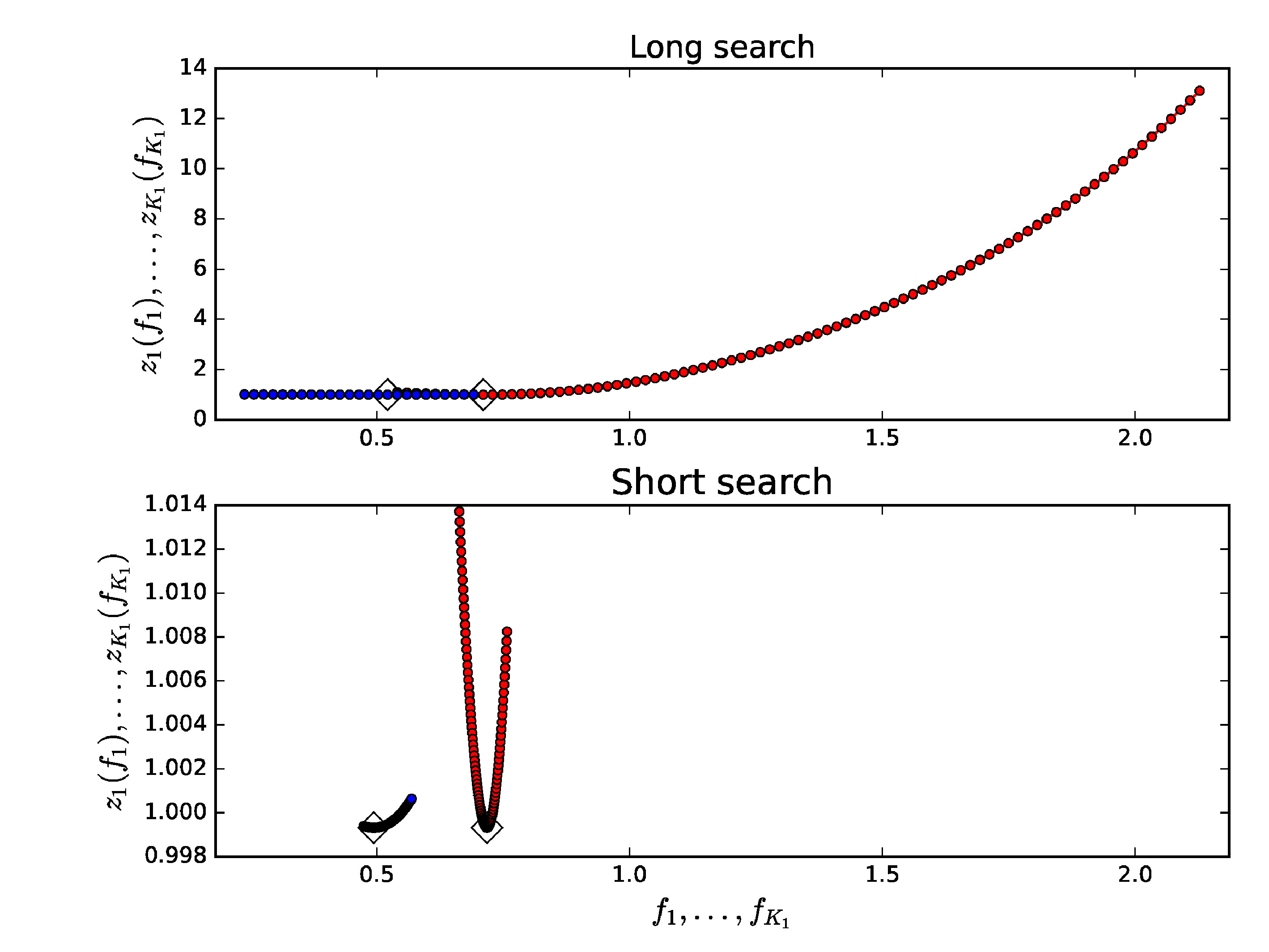
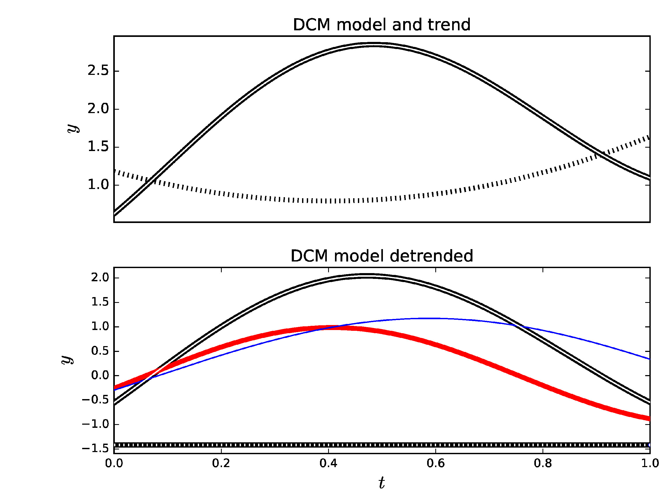
              (a)            (c)

              (b)            (d)

 

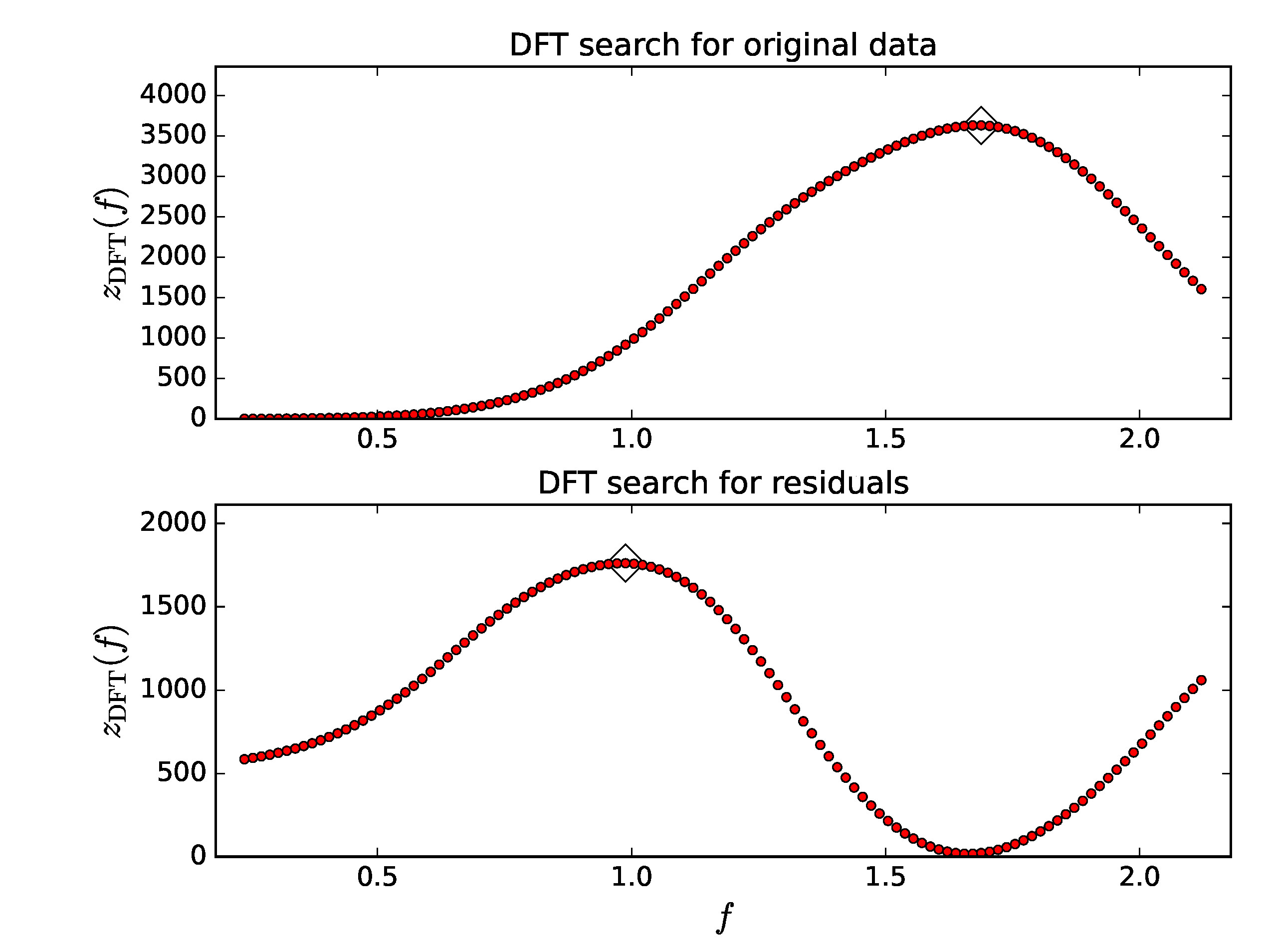
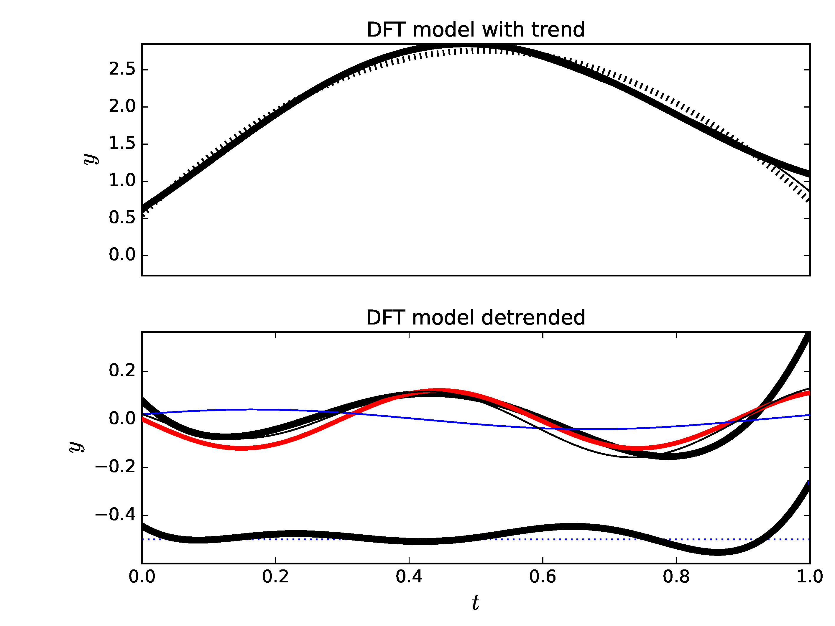
              (e)            (g)

              (f)            (h)

Figure 5: Model 5 (Table 5: $n=10~000$, ${\mathrm{SN}}=10~000$ simulation). Notations as in Figure 3. Best periods (diamonds) are explained in Section 3.5.

Table 6: Model 6. DCM analysis between $P_{\mathrm{min}}=0.053$ and $P_{\mathrm{max}}=0.480$. Notations as in Table 1.

(1)	(2)	(3)	(4)
	$n=50$	$n=50$	$n=100$
Model 6	${\mathrm{SN}}=10$	${\mathrm{SN}}=50$	${\mathrm{SN}}=100$
$P_{1}=0.16$	$0.15966\pm 0.00020$	$0.160022\pm 0.000021$	$0.160024\pm 0.000019$
$A_{1}=2.0$	$1.983\pm\pm 0.041$	$2.0031\pm 0.0086$	$2.0013\pm 0.0032$
$t_{\mathrm{1,min,1}}=0.0979$	$0.09868\pm 0.00057$	$0.097933\pm 0.000096$	$0.097934\pm 0.000079$
$t_{\mathrm{1,min,2}}=0.0225$	$0.02283\pm 0.00070$	$0.022563\pm 0.000077$	$0.022403\pm 0.000071$
$t_{\mathrm{1,max,1}}=0.1421$	$0.14241\pm 0.00064$	$0.142099\pm 0.000079$	$0.142100\pm 0.000077$
$t_{\mathrm{1,max,2}}=0.0575$	$0.05827\pm 0.00057$	$0.05761\pm 0.00011$	$0.057448\pm 0.000074$
$M_{0}=0$	$0.003\pm 0.012$	$-0.0055\pm 0.0026$	$0.00176\pm 0.00088$
Data file	Model6n50SN10.dat	Model6n50SN50.dat	Model6n100SN100.dat
Control file	dcmModel6n50SN10.dat	dcmModel6n50SN50.dat	dcmModel6n100SN100.dat

 

              (a)            (c)

              (b)            (d)

 

              (e)            (g)

              (f)            (h)

Figure 6: Model 6 (Table 6: $n=50$, ${\mathrm{SN}}=50$ simulation). Notations as in Figure 3. Best periods (diamonds) are explained in Section 3.6.

Table 7: Model 7. DCM analysis between $P_{\mathrm{min}}=0.4$ and $P_{\mathrm{max}}=3.6$. Notations as in Table 1.

(1)	(2)	(3)	(4)
	$n=100$	$n=1~000$	$n=10~000$
Model 7	${\mathrm{SN}}=5~000~000$	${\mathrm{SN}}=1~000~000$	${\mathrm{SN}}=1~000~000$
$P_{1}=1.2$	$1.19917\pm 0.00070$	$1.20000\pm 0.00063$	$1.20000\pm 0.00024$
$A_{1}=2.0$	$2.20\pm 0.20$	$1.94\pm 0.14$	$1.990\pm 0.057$
$t_{\mathrm{1,min,1}}=0.6892$	$0.6835\pm 0.0050$	$0.6900\pm 0.0043$	$0.6888\pm 0.0019$
$t_{\mathrm{1,min,2}}=0.1134$	$0.1235\pm 0.0098$	$0.1160\pm 0.0067$	$0.1128\pm 0.0026$
$t_{\mathrm{1,max,1}}=1.0195$	$1.0253\pm 0.0052$	$1.0176\pm 0.0039$	$1.0188\pm 0.0018$
$t_{\mathrm{1,max,2}}=0.3779$	$0.3705\pm 0.0082$	$0.3804\pm 0.0050$	$0.3780\pm 0.0020$
$P_{2}=1.4$	$1.4050\pm 0.0048$	$1.3986\pm 0.00034$	$1.3997\pm 0.0014$
$A_{2}=2.0$	$1.871\pm 0.098$	$2.049\pm 0.095$	$2.009\pm 0.040$
$t_{\mathrm{2,min,1}}=0.9262$	$0.938\pm 0.012$	$0.9231\pm 0.0090$	$0.9252\pm 0.0036$
$t_{\mathrm{2,min,2}}=0.2766$	$0.260\pm 0.016$	$0.281\pm 0.012$	$0.2771\pm 0.0046$
$t_{\mathrm{2,max,1}}=1.3109$	$1.3165\pm 0.0049$	$1.3105\pm 0.0039$	$1.3101\pm 0.0014$
$t_{\mathrm{2,max,2}}=0.5864$	$0.5817\pm 0.0037$	$0.5860\pm 0.0042$	$0.5865\pm 0.0015$
$M_{0}=1.0$	$0.950\pm 0.050$	$1.011\pm 0.035$	$1.002\pm 0.013$
$M_{1}=0.25$	$0.2447\pm 0.0067$	$0.2548\pm 0.0039$	$0.2509\pm 0.0018$
$M_{2}=0.5$	$0.551\pm 0.050$	$0.488\pm 0.035$	$0.498\pm 0.014$
Data file	Model7n100SN5000000.dat	Model7n1000SN1000000.dat	Model7n10000SN1000000.dat
Control file	dcmModel7n100SN5000000.dat	dcmModel7n1000SN1000000.dat	dcmModel7n10000SN1000000.dat

 

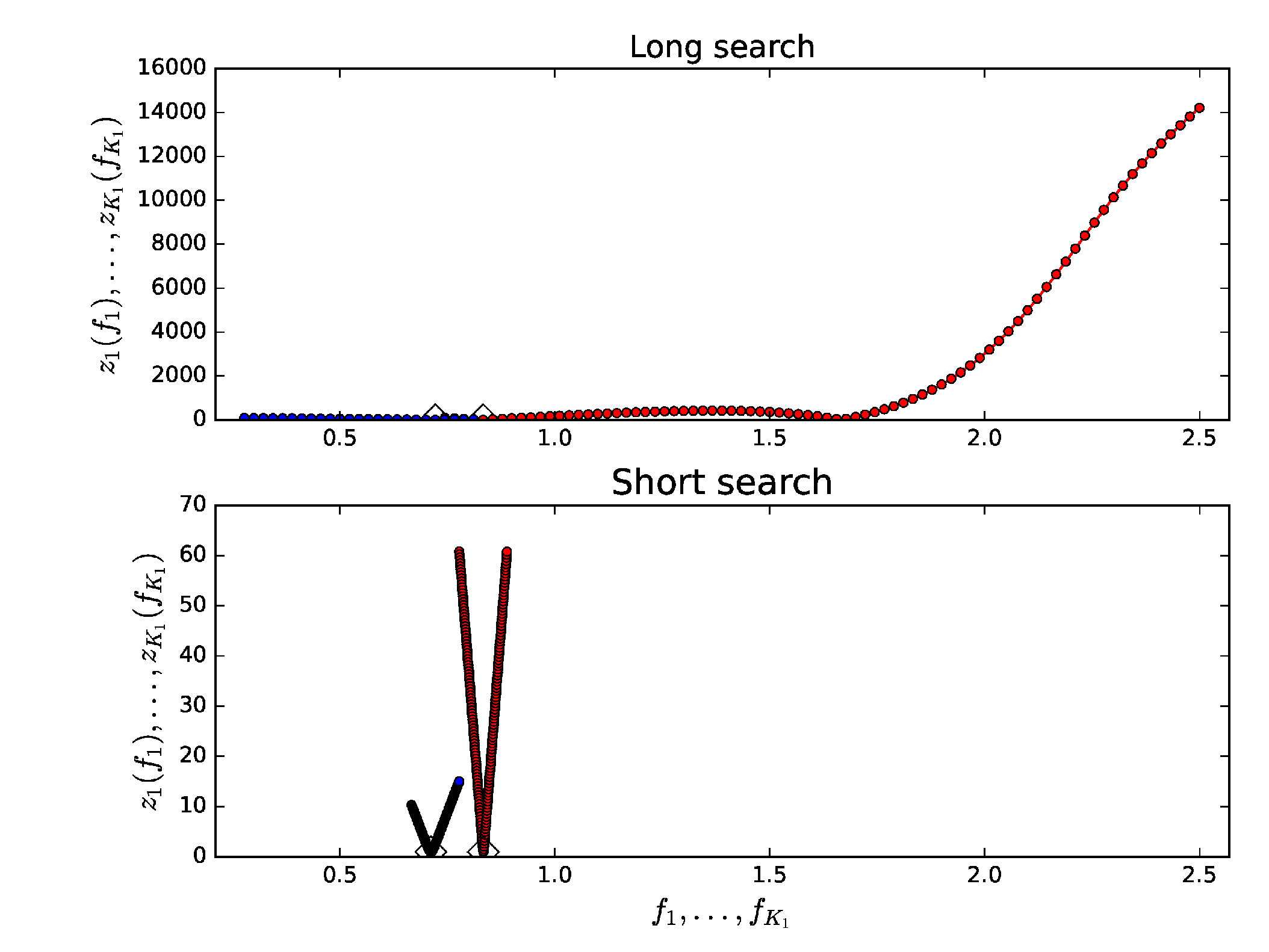
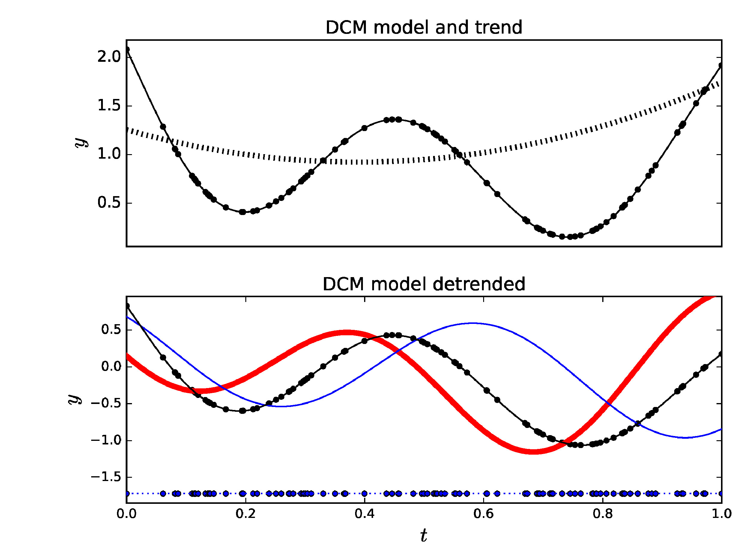
              (a)            (c)

              (b)            (d)

 

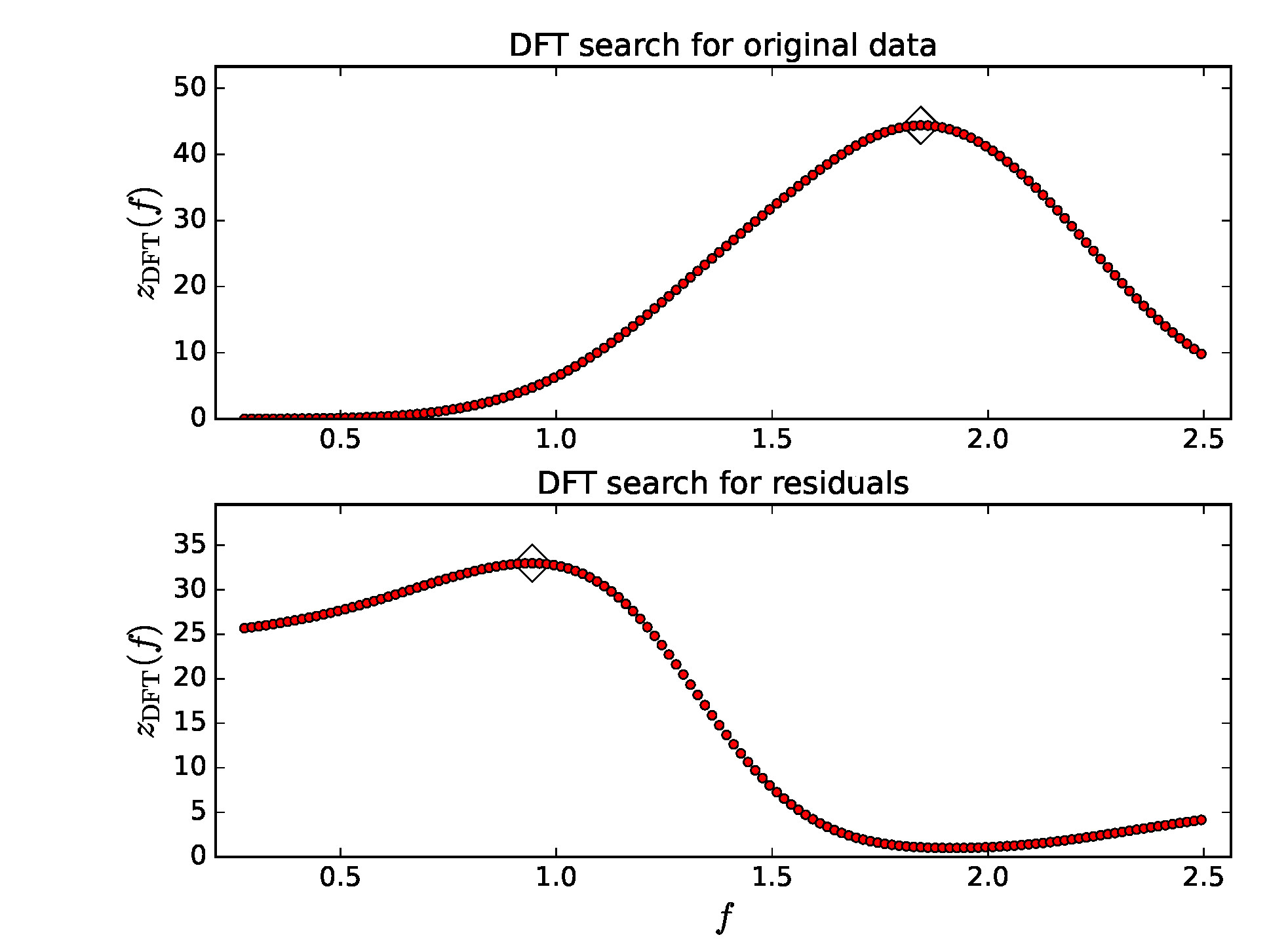
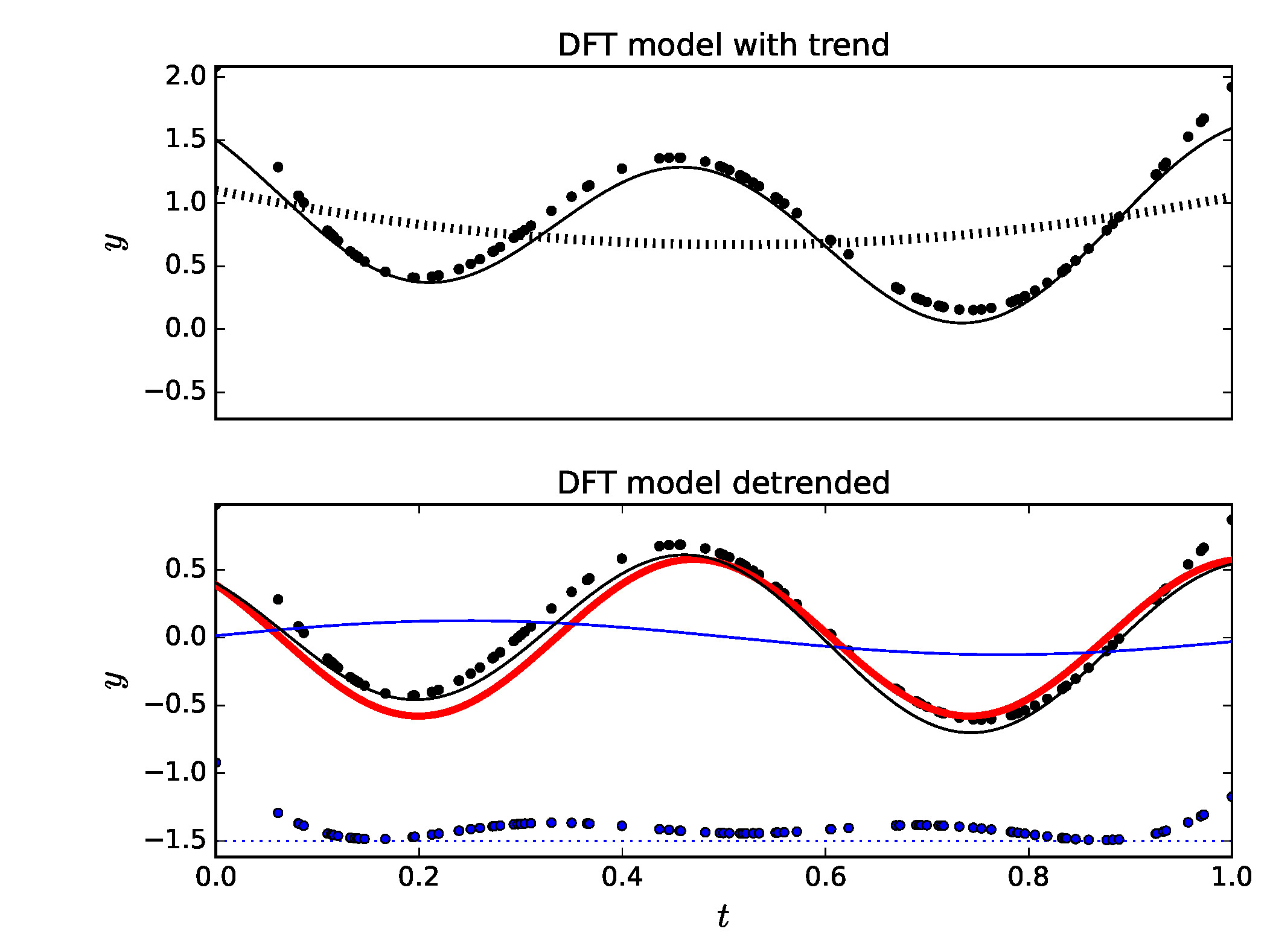
              (e)            (g)

              (f)            (h)

Figure 7: Model 7 (Table 7: $n=100$, ${\mathrm{SN}}=5~000~000$ simulation). otations as in Figure 3. Best periods (diamonds) are explained in Section 3.7.

3.5 Model 5

The mathematical equation

$$g(t) = (A_{1}/2)\cos{\left[{{2\pi(t-t_{\mathrm{1,max,1}})}\over{P_{1}}}\right]}$$

$$+ (A_{2}/2)\cos{\left[{{2\pi(t-t_{\mathrm{2,max,1}})}\over{P_{2}}}\right]}$$

$$+ M_{0}+M_{1}T+M_{2}T^{2}$$

for our fifth model for simulated data is the same for Model 4 (Equation 3.4). However, this new Model 5 differs from the earlier Model 4 because we use totally different $P_{1}$, $P_{2}$, $A_{1}$,$A_{2}$, $t_{\mathrm{1,max,1}}$, $t_{\mathrm{2,max,1}}$, $M_{0}$, $M_{1}$ and $M_{2}$ values (Table 5, Column 1). The simulated data sample is “too short” for both $P_{1}$ and $P_{2}$ periods (Equation 26). There is “a trend” $p(t)$ (Equation 27). The signal frequencies $f_{1}$ and $f_{2}$ are “too close” (Equation 28). The three main reasons that can cause the failure of DFT analysis are present. We perform the DCM and DFT time series analysis between $P_{\mathrm{min}}=P_{1}/3=0.47$ and $P_{\mathrm{max}}=3P_{1}=4.20$.

Model 5 has DCM orders $K_{1}=2$, $K_{2}=1$ and $K_{3}=2$. We give the DCM analysis results for different $n$ and ${\mathrm{SN}}$ combinations in Table 5 (Columns 2-4). The DCM fails to detect the correct $P_{1}$, $P_{2}$, …, $M_{1}$ and $M_{2}$ values for the the lowest $n=10~000$ and ${\mathrm{SN}}=1~000$ combination (Table 5, Column 2). This shows that the DCM can fail, just like any other time series analysis method, if the quality of data is too low. The DCM results for higher $n$ and ${\mathrm{SN}}$ combinations are correct (Table 5, Columns 3-4).

We show the DCM analysis results for one sample of Model 5 simulated data (Figures 5a-d: $n=10~000$ and ${\mathrm{SN}}=10~000$). The long and short DCM searches give $P_{1}=1.407$ and $P_{2}=1.917$ (Figure 5a: diamonds), and $P_{1}=1.393$ and $P_{2}=2.024$ (Figure 5b: Diamonds). The continuous line denoting the model $g(t)$ is totally covered by the black dots of $y_{i}$ data (Figure 5c). Therefore, we use white colour to highlight this DCM model $g(t)$ line. The detected polynomial trend $p(t)$ coefficients $M_{0}=0.81\pm 0.16$, $M_{1}=0.230\pm 0.013$ and $M_{2}=0.596\pm 0.084$ are correct (Figure 5c: dashed black line). We show the detrended DCM model $g(t)-p(t)$ (white continuous line), the detrended data $y(t_{i})-p(t_{i})$ (black dots), the signal $h_{1}(t)$ (red thick continuous line) and the signal $h_{2}(t)$ (blue thin continuous line) in Figure 5d. The DCM residuals (blue dots) are offset to the level of -1.5. These blue dots appear black because there are 10 000 of them. For obvious reasons, the -1.5 level of these residuals is highlighted by a white dotted line. The DCM model residuals are stable and show no trends.

The DFT detects the wrong periods for the original data (Figure 5e: diamond at $P_{1}=0.592$) and for the residuals (Figure 5f: diamond at $P_{2}=1.012$). The DFT estimates for the $p(t)$ trend, $M_{0}=2.758$, $M_{1}=0.091$ and $M_{2}=-2.120$, are also wrong (Figure 5g: dashed black line). The DFT model $g_{\mathrm{DFT}}(t)$ black continuous line deviates from the black dots of data $y_{i}$, especially in the end of the simulated data sample. The black dots denoting the detrended data $y(t_{i})-p_{\mathrm{DFT}}(t_{i})$ and the continuous black line denoting the detrended DFT model $g_{\mathrm{DFT}}(t)-p_{\mathrm{DFT}}(t)$ are shown in Figure 5h. The DFT model $g_{\mathrm{DFT}}(t)$ gives very low amplitudes for the pure sine signal $s_{\mathrm{y,DFT}}(t)$ (continuous thick red line) and pure sine signal $s_{\mathrm{\epsilon,DFT}}(t)$ (continuous thinner blue line). These amplitudes are far below the correct simulated values $A_{1}=A_{2}=2.$ The offset level for the DFT model residuals (blue dots) is -0.5. These residuals show strong trends.

The DCM analysis succeeds for Model 5 simulated data, but the DFT analysis fails.

3.6 Model 6

Our sixth data simulation model is

$$g(t) = c_{1}\cos{\left[{{2\pi t}\over{P_{1}}}\right]}$$

$$+ c_{2}\cos{\left[{{4\pi(t-c_{3})}\over{P_{1}}}\right]}+M_{0},$$

where $P=0.16$ and $M_{0}=0$. The coefficients $c_{1}=0.3655$, $c_{2}=0.7310$ and $c_{3}=0.3000$ determine the $A_{1}$, $t_{\mathrm{1,min,1}}$, $t_{\mathrm{1,min,2}}$, $t_{\mathrm{1,max,1}}$ and $t_{\mathrm{1,max,2}}$ values given in Table 6 (Column 1). This simulated data sample is not “too short” because $P_{1}<\Delta T$ (Equation 26). There is no trend because $p(t)=M_{0}=0$ (Equation 27). These simulated data contain only one signal (Equation 28). However, this simulation Model 6 is not a $K_{2}=1\texteuro$ pure sine model (Equation 29). This double wave simulation model has two unequal minima and maxima. Its DCM orders are $K_{1}=1$, $K_{2}=2$ and $K_{3}=0$. We perform the DCM and DFT time series analysis between $P_{\mathrm{min}}=P_{1}/3=0.053$ and $P_{\mathrm{max}}=3P_{1}=0.480$.

The DCM time series analysis results for different $n$ and ${\mathrm{SN}}$ combinations are given in Table 6 (Columns 2-4). The DCM detects the correct $P_{1}$, $A_{1}$, $t_{\mathrm{1,min,1}}$ $t_{\mathrm{1,min,2}}$ $t_{\mathrm{1,max,1}}$ $t_{\mathrm{1,max,2}}$ and $M_{0}$ values even for the lowest $n=50$ and ${\mathrm{SN}}=10$ combination. We demonstrate the DCM analysis results for simulated data having $n=50$ and ${\mathrm{SN}}=50$ (Figures 6a-d). The long and short searches give $P_{1}=0.159$ (Figure 6a: diamond) and $P_{1}=0.160$ (Figure 6b: diamond). The DCM model $g(t)$ black line covers the black dots denoting the data $y_{i}$ (Figure 6c). The "trend" at $p(t)=M_{0}=-0.0055\pm 0.0026$ is correct. The detrended model $g(t)-p(t)$ (black continuous line), the pure sine signal $h_{1}(t)$ (red thick continuous line) and the detrended data $y(t_{i})-p(t_{i})$ (black dots) are displayed in Figure 6d. The thick continuous red line stays under the thin continuous black line because $h_{1}(t)=g(t)-p(t)$. The DCM residuals (blue dots) are offset to the level of -1.8 (blue dotted line). These residuals show no trends and their level is stable.

The DFT detects the wrong period $P_{1}=0.080$ (Figure 6e: Diamond). This results is exactly half of the correct simulated value $P_{1}=0.160$. The reason for this “detection” is that the double wave dominates because $c_{2}=2c_{1}$ in Model 6 (Equation 3.7). The DFT mean level estimate $M_{0}=-0.172$ fails (Figure 6f: Dashed black line). The DFT analysis of the residuals $\epsilon_{i}=$ $y(t_{i})-[s_{\mathrm{y,DFT}}(t_{i})+p_{\mathrm{DFT}}(t_{i})]$ gives $P_{2}=0.161$, which is nearly equal to the correct simulated $P_{1}=0.160$ value. The black dots denoting the data $y_{i}$ show minor deviations from continuous black line denoting the DFT model $g_{\mathrm{DFT}}(t)$ (Figure 6g). The detrended model $g_{\mathrm{DFT}}(t)-p_{\mathrm{DFT}}(t)$ (continuous black line), the detrended data $y(t_{i})-p_{\mathrm{DFT}}(t_{i})$ (black dots) and the signal $s_{\mathrm{y,DFT}}(t)$ (continuous thick red line) are shown in Figure 6h. The DFT analysis residuals (blue dots) are offset to the level of -1.5 (blue dotted line). These residuals display trends.

We conclude that the DFT “detects” the $P_{1}/2$ and $P_{1}$ periods, where $P_{1}$ is the correct simulated period value. However, the DFT two signal model is not the correct model for these Model 6 simulated data, which contain only one signal. If the correct period is $P$ and the correct model is a double wave $(K_{2}=2)$, the DCM pure sine model $(K_{1}=1)$ analysis can also give the values $P/2$ and $P$ [14].

The DCM analysis succeeds for Model 6 simulated data. The DFT analysis fails.

3.7 Model 7

Our seventh simulation model is

$$g(t) = c_{1}\cos{\left[{{2\pi t}\over{P_{1}}}\right]}+c_{2}\cos{\left[{{4\pi(t-c_{3})}\over{P_{1}}}\right]}$$

$$+ c_{4}\cos{\left[{{2\pi t}\over{P_{2}}}\right]}+c_{5}\cos{\left[{{4\pi(t-c_{6})}\over{P_{2}}}\right]}$$

$$+ M_{0}+M_{1}T+M_{2}T^{2}$$

where $T=[2(t-t_{\mathrm{mid}})]/\Delta T$, $P_{1}=1.2$, $P_{2}=1.4$, $M_{0}=1$ $M_{1}=0.25$ and $M_{2}=0.5$. The coefficients $c_{1}=0.3687$, $c_{2}=0.7374$, $c_{3}=0.4000$, $c_{4}=0.3708$, $c_{5}=0.7416$ and $c_{6}=0.6000$ determine the $A_{1}$, $t_{\mathrm{1,min,1}}$, $t_{\mathrm{1,min,2}}$, $t_{\mathrm{1,max,1}}$, $t_{\mathrm{1,max,2}}$, $A_{2}$, $t_{\mathrm{2,min,1}}$, $t_{\mathrm{2,min,2}}$, $t_{\mathrm{2,max,1}}$ and $t_{\mathrm{2,max,2}}$ values given in Table 7 (Column 1). This simulated data sample is “too short” because $\Delta T<P_{1}<P_{2}$ (Equation 26). The parabolic $p(t)$ represents “a trend” (Equation 27). The signal frequencies $f_{1}$ and $f_{2}$ are “too close” because $\Delta f=f_{1}-f_{2}=0.12<f_{0}=1$ (Equation 28). The two $h_{1}(t)$ and $h_{2}(t)$ signals are not “pure sines” (Equation 29). These signals are double waves having two unequal minima and maxima. All four main reasons that can cause the failure of DFT analysis are present (Equations 26-29). Our DCM and DFT time series analysis of Model 7 simulated data is performed between $P_{\mathrm{min}}=P_{1}/3=0.4$ and $P_{\mathrm{max}}=3P_{1}=3.6$.

The DCM orders of Model 7 are $K_{1}=2$, $K_{2}=2$ and $K_{3}=2$. This model has $\eta=13$ free parameters (Equation 8). We give the DCM analysis results for different $n$ and ${\mathrm{SN}}$ combinations in Table 7 (Columns 2-4). The DCM analysis results are displayed for one sample of Model 7 simulated data (Figures 7a-d: $n=100$ and ${\mathrm{SN}}=5~000~000$). Since there are $\eta=13$ free model parameters, this $n=100$ sample is quite small for time series analysis. The long and short DCM searches give $P_{1}=1.200$ and $P_{2}=1.385$ (Figure 7a: diamonds), and $P_{1}=1.199$ and $P_{2}=1.405$ (Figure 7b: Diamonds). The black $g(t)$ model line goes through all black $y_{i}$ data dots (Figure 7c). The DCM detects the correct polynomial trend $p(t)$ coefficients $M_{0}=0.950\pm 0.050$, $M_{1}=0.2447\pm 0.0067$ and $M_{2}=0.551\pm 0.050$ (Figure 7c: dashed black line). The detrended DCM model $g(t)-p(t)$ (white continuous line), the detrended data $y(t_{i})-p(t_{i})$ (black dots), the signal $h_{1}(t)$ (red thick continuous line) and the signal $h_{2}(t)$ (blue thin continuous line) are displayed in Figure 7d. The $n=100$ residuals (blue dots) are offset to the level of -1.8 (dotted blue line). These DCM model residuals are small and their level is stable. These results confirm that the DCM time series analysis method can detect complex non-linear models $(\eta=13)$ from very small data samples $(n=100)$, if these data are extremely accurate $({\mathrm{SN}}=5~000~000).$

The DFT time series analysis gives the wrong periods for the original data (Figure 7e: diamond at $P_{1}=0.542$ and for the residuals (Figure 7f: diamond at $P_{2}=1.059$. The DFT also gives wrong $p(t)$ trend coefficients $M_{0}=0.670$, $M_{1}=-0.025$ and $M_{2}=0.406$ (Figure 7g: dashed black line). The DFT model $g_{\mathrm{DFT}}(t)$ (black continuous line) deviates from the data $y_{i}$ (black dots). This deviation is largest at the beginning and the end of the simulated data sample. In our Figure 7h, the black dots denote the detrended data $y(t_{i})-p_{\mathrm{DFT}}(t_{i})$, the continuous black line denotes the detrended DFT model $g_{\mathrm{DFT}}(t)-p_{\mathrm{DFT}}(t)$ and the continuous thick red line denotes pure sine signal $s_{\mathrm{y,DFT}}(t)$ detected from the original data. The DFT model $g_{\mathrm{DFT}}(t)$ gives very low amplitude for the pure sine signal $s_{\mathrm{\epsilon,DFT}}(t)$ detected from the residuals (continuous thinner blue line). The correct simulated peak to peak amplitude for this second signal is much larger, $A_{2}=2.$ The DFT model residuals (blue dots) are offset to -1.5 level and show strong trends.

The DCM time series analysis succeeds for Model 7 simulated data. The DFT time series analysis fails, as predicted by Equations 26-29.

Table 8: Fisher tests. DCM analysis of Model 1 simulated data ($n=100,{\mathrm{SN}}=100$, data file Model1n100SN100). (1) Simple model: Model number $\mathcal{M}$, model $g_{K_{1},K_{2},K_{3}}$, number of free parameters $\eta$, chi-square $\chi^{2}$ and control file name. (2-8) Complex model: Hypothesis H₀ rejected $\uparrow$ (Complex model better), Hypothesis H₀ not rejected $\leftarrow$ (Simple model better), test statistic $F$ and critical level $Q_{\mathrm{F}}$.

(1) (2) (3) (4) (5) (6) (7) (8) Complex model Simple model $\mathcal{M}$=2 $\mathcal{M}$=3 $\mathcal{M}$=4 $\mathcal{M}$=5 $\mathcal{M}$=6 $\mathcal{M}$=7 $\mathcal{M}$=8 $\mathcal{M}$=1 $\uparrow$ $\uparrow$ $\uparrow$ $\uparrow$ $\uparrow$ $\uparrow$ $\uparrow$ $g_{1,,1,-1}$ $F=733$ $F=367$ $F=242$ $F=242$ $F=180$ $F=142$ $F=121$ $\eta=3$,$\chi^{2}=738$ $Q_{\mathrm{F}}<\!10^{-16}$ $Q_{\mathrm{F}}<\!10^{-16}$ $Q_{\mathrm{F}}<\!10^{-16}$ $Q_{\mathrm{F}}<\!10^{-16}$ $Q_{\mathrm{F}}<\!10^{-16}$ $Q_{\mathrm{F}}<\!10^{-16}$ $Q_{\mathrm{F}}<\!10^{-16}$ dcmModel1K11-1.dat $\mathcal{M}$=2 - $\leftarrow$ $\leftarrow$ $\leftarrow$ $\leftarrow$ $\leftarrow$ $\leftarrow$ $g_{1,1,0}$ - $F=1.0451$ $F=0.5404$ $F=0.5159$ $F=0.3553$ $F=0.2784$ $F=0.7686$ $\eta=4$,$\chi^{2}=84.7422$ - $Q_{\mathrm{F}}=0.309$ $Q_{\mathrm{F}}=0.584$ $Q_{\mathrm{F}}=0.599$ $Q_{\mathrm{F}}=0.785$ $Q_{\mathrm{F}}=0.891$ $Q_{\mathrm{F}}=0.575$ dcmModel1K110.dat $\mathcal{M}$=3 - - $\leftarrow$ $\leftarrow$ $\leftarrow$ $\leftarrow$ $\leftarrow$ $g_{1,1,,1}$ - - $F=0.0464$ $F=-0.0021$ $F=0.0213$ $F=0.0336$ $F=0.7027$ $\eta=5$,$\chi^{2}=83.8104$ - - $Q_{\mathrm{F}}=0.830$ $Q_{\mathrm{F}}=1$ $Q_{\mathrm{F}}=0.979$ $Q_{\mathrm{F}}=0.992$ $Q_{\mathrm{F}}=0.592$ dcmModel1K111.dat $\mathcal{M}$=4 - - - $\leftarrow$ $\leftarrow$ $\leftarrow$ $\leftarrow$ $g_{1,1,2}$ - - - No test $F=-0.0033$ $F=0.0277$ $F=0.9215$ $\eta=6$,$\chi^{2}=83.7686$ - - - $Q_{\mathrm{F}}=1$ $Q_{\mathrm{F}}=0.973$ $Q_{\mathrm{F}}=0.434$ dcmModel1K112.dat $\mathcal{M}$=5 ${\color[rgb]{0,0,0}{\bf\mathrm{UM}}}:{\color[rgb]{0,0,0}{\bf\mathrm{AD}}}$ - - - - $\leftarrow$ $\leftarrow$ $\leftarrow$ $g_{2,1,-1}$ - - - - $F=0.0447$ $F=0.0515$ $F=0.9377$ $\eta=6$,$\chi^{2}=83.8123$ - - - - $Q_{\mathrm{F}}=0.833$ $Q_{\mathrm{F}}=0.950$ $Q_{\mathrm{F}}=0.426$ dcmModel1K21-1.dat $\mathcal{M}$=6 ${\color[rgb]{0,0,0}{\bf\mathrm{UM}}}:{\color[rgb]{0,0,0}{\bf\mathrm{IF}}},{\color[rgb]{0,0,0}{\bf\mathrm{AD}}}$ - - - - - $\leftarrow$ $\leftarrow$ $g_{2,1,0}$ - - - - - $F=0.0587$ $F=1.3840$ $\eta=7$,$\chi^{2}=83.7716$ - - - - - $Q_{\mathrm{F}}=0.809$ $Q_{\mathrm{F}}=0.256$ dcmModel1K210.dat M=7 ${\color[rgb]{0,0,0}{\bf\mathrm{UM}}}:{\color[rgb]{0,0,0}{\bf\mathrm{IF}}},{\color[rgb]{0,0,0}{\bf\mathrm{AD}}}$ - - - - - - $\leftarrow$ $g_{2,1,1}$ - - - - - - $F=2.7081$ $\eta=8$,$\chi^{2}=83.7176$ - - - - - - $Q_{\mathrm{F}}=0.103$ dcmModel1K211.dat - $\mathcal{M}$=8 ${\color[rgb]{0,0,0}{\bf\mathrm{UM}}}:{\color[rgb]{0,0,0}{\bf\mathrm{IF}}},{\color[rgb]{0,0,0}{\bf\mathrm{AD}}}$ - - - - - - - $g_{2,1,2}$ - - - - - - - $\eta=9$,$\chi^{2}=81.2721$ - - - - - - - dcmModel1K212.dat -

3.8 Best model

The $K_{1}$, $K_{2}$ and $K_{3}$ orders of the best model are not necessarily known when some time series analysis method is applied to the real data. We know a priori the best DCM and DFT model orders for the simulated data of Models 1-7 (Sections 3.1-3.7). It could be argued that our DCM analysis succeeds only for this reason.

All alternative $K_{1}$, $K_{2}$ and $K_{3}$ order models are nested. For example, the simple one signal $K_{1}=1$ model $g_{1}(t)$ is a special case of the complex two signal $K_{1}=2$ model $g_{2}(t)$ having $A_{2}=0$. We use the Fisher-test to compare any pair of simple $g_{1}(t)$ and complex $g_{2}(t)$ models. The model parameters (Equation 13: $R_{1},R_{2}$ ), (Equation 14: $\chi_{1}$,$\chi_{2}$) and (Equation 8: $\eta_{1}<\eta_{2}$) give the test statistic of Fisher-test

$$F_{R} = \left({{R_{1}}\over{R_{2}}}-1\right)\left({{n-\eta_{2}-1}\over{\eta_{2}-\eta_{1}}}\right)$$ (37)

$$F_{\chi} = \left({{\chi_{1}^{2}}\over{\chi_{2}^{2}}}-1\right)\left({{n-\eta_{2}-1}\over{\eta_{2}-\eta_{1}}}\right).$$ (38)

The Fisher-test is based on the null hypothesis

• $H_{\mathrm{0}}$: “The complex model $g_{2}(t)$ does not provide a significantly better fit to the data than the simple model $g_{\mathrm{1}}(t)$.”

Under this hypothesis, the $F_{R}$ and $F_{\chi}$ test statistic parameters have an $F$ distribution with $\nu_{1}=\eta_{2}-\eta_{1}$ and $\nu_{2}=n-\eta_{2}$ degrees of freedom [4]. The critical level $Q_{F}=P(F_{R}\geq F)$ or $Q_{F}=P(F_{\chi}\geq F)$ is the probability that $F_{R}$ or $F_{\chi}$ exceeds the numerical value $F$. If

$$Q_{F}<\gamma_{F}=0.001,$$ (39)

we reject the $H_{0}$ hypothesis, which means that the complex $g_{2}(t)$ model is better than the simple $g_{1}(t)$ model. The pre-assigned significance level $\gamma_{F}=0.001$ represents the probability that we falsely reject the $H_{0}$ hypothesis when it is in fact true.

Larger $F_{R}$ or $F_{\chi}$ values have smaller $Q_{F}$ critical levels. Hence, the probability for the $H_{0}$ hypothesis rejection increases when $F_{R}$ or $F_{\chi}$ increases. If the number of complex model free parameters $\eta_{2}$ increases, the $R_{2}$ or $\chi^{2}_{2}$ values decrease. This increases the $F_{R}$ or $F_{\chi}$ values because the terms $(R_{1}/R_{2}-1)$ or $(\chi^{2}_{1}/\chi^{2}_{2}-1)$ (Equations 37 and 38: first terms). At the same time, the $(n-\eta_{2}-1)/(\eta_{2}-\eta_{1})$ penalty term decreases (Equations 37 and 38: second terms), and this decreases the $F_{R}$ or $F_{\chi}$ values. This penalty term prevents the use of too high $\eta_{2}$ values (too complex models).

Here, we illustrate how the Fisher-test finds the best model from a group of numerous alternative nested DCM models. The Fisher-test is used to find the best model for the simulated data of Model 1 combination $n=100$ and ${\mathrm{SN}}=100$ (Table 1: column 4). In other words, we assume that the correct DCM model orders $K_{1}$, $K_{2}$ and $K_{3}$ are unknown, which can be the case for real data. The eight tested models contain one or two signals, and no trend or a constant trend or a linear trend or a parabolic trend. We compare all these eight models $\mathcal{M}$=1-8 against each other (Table 8). The special model number notation“$\mathcal{M}$” is used because the notations “$M_{0}$, …, $M_{K_{3}}$” have already been reserved for the $p(t)$ trend.

Model $\mathcal{M}$=2 has the known correct Model 1 orders $K_{1}=1$, $K_{2}=1$ and $K_{3}=0$. For example, the Fisher-test between the simple model $\mathcal{M}$=1 $(\eta=3$, $\chi^{2}=738)$ and the complex model $\mathcal{M}$=2 $(\eta=4$, $\chi^{2}=84.7422)$ gives $F=733$ (Equation 38). The critical level for this very large $F$ value is extremely significant, $Q_{\mathrm{F}}<\!10^{-16}$. This means that the $H_{0}$ hypothesis must be rejected, and the complex $\mathcal{M}$=2 model is certainly better than the simple $\mathcal{M}$=1 model (Equation 39). The upward arrow “$\uparrow$” in Table 8 indicates that $\mathcal{M}$=2 model is a better model than $\mathcal{M}$=1 model. A closer look at Table 8 reveals that $\mathcal{M}$=2 model is better than all other models because the “$\uparrow$” and “$\leftarrow$” arrows of all other models point toward $\mathcal{M}$=2 model. There is no need to test models having more than two signals because all two signal $\mathcal{M}$=5-8 models are already unstable (Table 8:”${\color[rgb]{0,0,0}{\bf\mathrm{UM}}}$”). The Fisher-test finds the correct DCM model for Model 1 simulated data.

Table 9: Fisher tests for Model 1 $n=100,{\mathrm{SN}}=100$ simulated data (electronic data file Model1n100SN100). (1) Polynomial model. (2) DCM model $g_{1,1,0}$. Note that $\mathcal{M}$=1-3  polynomials represent simple models, and $\mathcal{M}$=5-8  polynomials represent complex models. Otherwise as in Table 8.

(1)	(2)
	$g_{1,1,0}$
Polynomial	$\eta=4,\chi^{2}=84.7422$
$\mathcal{M}$=1	$\uparrow$
$g(t)=p(t,K_{3}=0)$	$F=63218$
$\eta=1$, $\chi^{2}=169260$	$Q_{\mathrm{F}}<\!10^{-16}$
$\mathcal{M}$=2	$\uparrow$
$g(t)=p(t,K_{3}=1)$	$F=54366$
$\eta=2$, $\chi^{2}=97076$	$Q_{\mathrm{F}}<\!10^{-16}$
$\mathcal{M}$=3	$\uparrow$
$g(t)=p(t,K_{3}=2)$	$F=1945$
$\eta=3$, $\chi^{2}=1820$	$Q_{\mathrm{F}}<\!10^{-16}$
$\mathcal{M}$=4	$\uparrow$
$g(t)=p(t,K_{3}=3)$	No test
$\eta=4$, $\chi^{2}=469$
$\mathcal{M}$=5	$\uparrow$
$g(t)=p(t,K_{3}=4)$	$F=-0.3718$
$\eta=5$, $\chi^{2}=85.0787$	$Q_{\mathrm{F}}=1$
$\mathcal{M}$=6	$\uparrow$
$g(t)=p(t,K_{3}=5)$	$F=0.3403$
$\eta=6$, $\chi^{2}=84.1265$	$Q_{\mathrm{F}}=0.712$
$\mathcal{M}$=7	$\uparrow$
$g(t)=p(t,K_{3}=6)$	$F=0.3524$
$\eta=7$, $\chi^{2}=83.7794$	$Q_{\mathrm{F}}=0.787$
$\mathcal{M}$=8	$\uparrow$
$g(t)=p(t,K_{3}=7)$	$F=0.9394$
$\eta=8$, $\chi^{2}=81.3819$	$Q_{\mathrm{F}}=0.445$

In the above example, the Fisher-test finds the correct number of signals $(K_{1})$ and the correct trend $(K_{3})$ for the pure sine signal alternative $(K_{2}=1)$. We do not test the double wave signal alternative $(K_{2}=2)$ against the pure sine signal alternative $(K_{1}=1)$ because the number of tested models would increase from 8 to 16, and Table 8 would become excessively large. One example of testing the $K_{2}=1$ and $K_{2}=2$ signal models against each other can be found in Jetsu [14, Table 4].

We conclude that the best model for the real data can be found by applying the Fisher-test to any arbitrary number of different nested DCM or DFT models.

3.9 Significance estimates

The Fisher-test gives the critical level $Q_{\mathrm{F}}$ for rejecting the $H_{0}$ hypothesis (Equation 39). After the detection of the first strongest signal, the values $Q_{\mathrm{F}}$ of these critical levels increase for the next detected weaker signals. Typical examples can be found in Jetsu 2025 (Tables S5-S16). No new signals are detected when $Q_{\mathrm{F}}>\gamma=0.001$ because the critical level exceeds the pre-assigned significance level and the $H_{0}$ hypothesis is no longer rejected.

The Fisher test critical level $Q_{\mathrm{F}}$ is the significance estimate for each signal detected after the first signal. However, this Fisher-test process gives no significance estimate for the first detected signal.

We estimate the critical level $Q_{\mathrm{F}}$ for the first detected signal $h_{1}(t)$ by testing the alternative that there are no signals in the data. The “no signal hypothesis” is

$$h(t)=0\Rightarrow h_{1}(t)=0\Rightarrow g(t)=p(t).$$ (40)

In Model 1 simulated data combination $n=100$ and ${\mathrm{SN}}=100$, the correct model is $g_{1,1,0}(t)$. We use the Fisher-test to compare this correct $g_{1,1,0}(t)$ model to different polynomial models $g(t)=p(t)$ having $K_{3}=0,1,..,7$ (Table 9).

The $\mathcal{M}$=1, 2 and 3 models have less free parameters than the correct $g_{1,1,0}(t)$ model, but the $\chi^{2}$ values of these three polynomial models are so large that the Fisher-test is merely a formality. The $\mathcal{M}$=4 model has the same number of free parameters as the correct $g_{1,1,0}(t)$ model, but the comparison of $\chi^{2}$ values reveals that this third order $p(t)$ polynomial is not the correct model for the data. The next model $\mathcal{M}$=5 has more free parameters than the correct $g_{1,1,0}(t)$ model. This fourth order $p(t)$ polynomial $\mathcal{M}$=5 model must be rejected because it has a larger $\chi^{2}$ value than the correct $g_{1,1,0}(t)$ model. The critical levels $Q_{\mathrm{F}}\gg\gamma=0.001$ for the remaining $\mathcal{M}$=6, 7 and 8 polynomial models are so large that these models must also be rejected. The results in Table 9 confirm the “no signal hypothesis” (Equation 40) rejection. The analysed Model 1 simulated data must contain at least the $h_{1}(t)$ pure sine signal. For the constant, linear or parabolic $p(t)$ trend alternatives, the critical level for this $h_{1}(t)$ signal is $Q_{\mathrm{F}}<\!10^{-16}$.

There is no need to discuss the DFT significance estimates [11, their Equation 22] because this method fails to detect the correct Model 1 period.

Table 10: DCM time series analysis between $P_{\mathrm{min}}=0.53$ and $P_{\mathrm{max}}=4.80$ for predictive data (Model = 3 combination $n=50$ and ${\mathrm{SN}}=10$ simulated data: first forty observations). (1) Model. (2) Predictive data test statistic $z$ (Equation 16). (3) Predicted data test statistic $z_{\mathrm{pred}}$ (Equation 3.10). (4) Data file. (5) Control file. (6) Figure where prediction is shown.

(1)	(2)	(3)	(4)	(5)	(6)
Model	$z$	$z_{\mathrm{pred}}$	Data file	Control file	Figure
$g_{1,1,0}$	2.27	8.61	Model3n40SN10.dat	dcmModel3K110.dat	8a
$g_{2,1,0}$	0.76	0.88	Model3n40SN10.dat	dcmModel3K210.dat	8b
$g_{3,1,0}$	0.70	0.91	Model3n40SN10.dat	dcmModel3K310.dat	8c

 

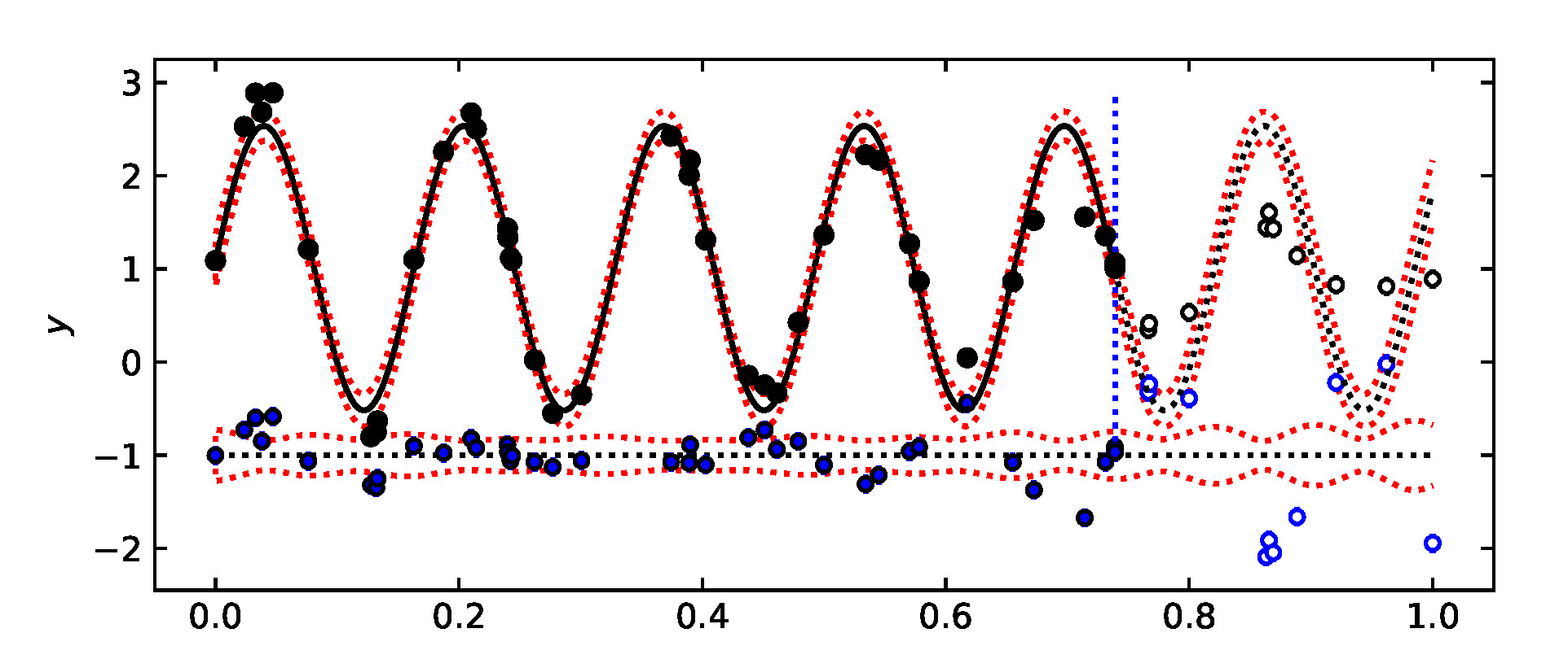
                      (a)

 

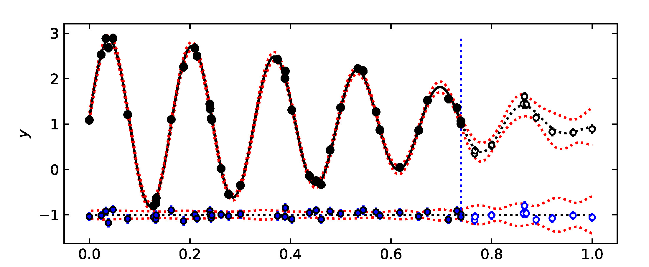
                      (b)

 

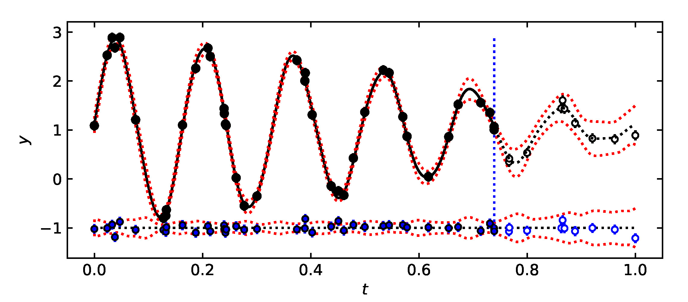
                      (c)

Figure 8: DCM model prediction (Model 3 simulated data for combination $n=50$ and ${\mathrm{SN}}=10$: first forty observations are predictive data). (a) One signal model $g_{1,1,0}$ results. Predictive data are $t_{i}$, $y_{i}$ and $\sigma_{i}$ ($n=40$ black dots) and predicted data are ten last observations $t_{i}^{\prime}$, $y_{i}^{\prime}$ and $\sigma_{i}^{\prime}$ ($n=10$ open black dots). Continuous black line of predictive data model $g(t,\bm{\beta}_{\mathrm{pred}})$ ends to vertical dotted blue line, where dotted black line of predicted model $g^{\prime}(t,\bm{\beta}_{\mathrm{pred}})$ begins. Dotted red line denotes $\pm 3\sigma$ errors of both models. Residuals of predictive data model $\epsilon_{i}=y_{i}-g_{i}$ (blue dots), residuals of predicted data model $\epsilon_{i}=^{\prime}y_{i}^{\prime}-g_{i}^{\prime}$ (open blue dots) and $\pm 3\sigma$ errors of both models (red dotted line) are offset to level -1 (blue dotted line). (b) Two signal model $g_{2,1,0}$ results. Otherwise as in “a”. (c) Three signal model $g_{3,1,0}$ results. Otherwise as in “a”.

3.10 Prediction

There are numerous techniques for predicting (forecasting) a time series [e.g., 10, 12]. The DCM model $g(t_{i},\bm{\beta})$ can be used to predict. We divide all data into the predictive data and the predicted data. The time points, the observations and the errors of these samples are

• $n$ predictive data values $t_{i}$, $y_{i}$ and $\sigma_{i}$

• $n^{\prime}$ predicted data values $t_{i}^{\prime}$, $y_{i}^{\prime}$ and $\sigma_{i}^{\prime}$

The DCM gives the best predictive data model

$$g_{i}=g(t_{i},\bm{\beta}_{\mathrm{pred}}),$$ (41)

where $\bm{\beta}_{\mathrm{pred}}$ are the free parameter values. The $t_{\mathrm{mid,pred}}\!=\!(t_{n}\!+\!t_{1})/2$ and $\Delta T_{\mathrm{pred}}\!=\!t_{n}\!-\!t_{1}$ values are computed from the predictive data time points $t_{i}$.

The predicted data model values are

$$g^{\prime}_{i} = g(t^{\prime}_{i},\bm{\beta}_{\mathrm{pred}}),$$ (42)

where $t_{\mathrm{mid}}=t_{\mathrm{mid,pred}}$ and $\Delta T=\Delta T_{\mathrm{pred}}$. We do not compute “new” $t_{\mathrm{mid}}$ and $\Delta T$ values from the predicted data time points $t^{\prime}_{i}$ because the correct $g^{\prime}_{i}$ values are obtained only from the $\bm{\beta}_{\mathrm{pred}}$, $t_{\mathrm{mid,pred}}$ and $\Delta T_{\mathrm{pred}}$ combination of Equation 41. The $n^{\prime}$ predicted data model residuals

$$\epsilon^{\prime}_{i}=y^{\prime}_{i}-g^{\prime}_{i}$$

give the predicted data test statistic

$$z_{\mathrm{pred}} =$$ z test statistic for predicted

data $$t^{\prime}_{i} y^{\prime}_{i} \sigma^{\prime}_{i}$$, and (Equation 15 or 16).

This parameter $z_{\mathrm{pred}}$ measures how well the prediction (Equation 42) obtained from the predictive data works for the predicted data. If the DCM detects a new signal from the predictive data, there are two alternatives:

• If this new signal is real, the $z_{\mathrm{pred}}$ value of predicted data decreases.

• If this new signal is unreal, the $z_{\mathrm{pred}}$ value of predicted data increases.

This “Prediction-test” technique revealed at least five real signals in the sunspot record (Jetsu 2025).

We compute the $z_{\mathrm{pred}}$ parameter value from the known predicted data $t^{\prime}_{i}$, $y^{\prime}_{i}$ and $\sigma^{\prime}_{i}$ values (Equation 3.10) . Predictions are possible even if all $t^{\prime}_{i}$, $y^{\prime}_{i}$ or $\sigma^{\prime}_{i}$ predicted data values are unknown. In this case, the $t_{i}$, $y_{i}$ and $\sigma_{i}$ values of all data can be used as predictive data. The best DCM model $g(t_{i},\bm{\beta}_{\mathrm{pred}})$ for all data determines the correct $\bm{\beta}_{\mathrm{pred}}$, $t_{\mathrm{mid,pred}}=(t_{n}+t_{1})/2$ and $\Delta T_{\mathrm{pred}}=t_{n}-t_{1}$ combination. The $n^{\prime}$ predicted data time points $t_{i}^{\prime}$ can be created for any arbitrary chosen time interval $\Delta T^{\prime}=t_{n}^{\prime}-t_{i}^{\prime}$. The $n^{\prime}$ predicted model $g_{i}^{\prime}=g^{\prime}_{i}(t_{i}^{\prime},\bm{\beta}_{\mathrm{pred}})$ values are obtained from Equation 42. These $g^{\prime}_{i}$ values can be used, for example, to compute the predicted mean level

$$m_{\mathrm{pred}}={{1}\over{n^{\prime}}}\sum_{i=1}^{n^{\prime}}g^{\prime}_{i}$$ (44)

during the chosen time interval $\Delta T^{\prime}=t_{n}^{\prime}-t_{1}^{\prime}$. Jetsu (2025) used this $m_{\mathrm{pred}}$ parameter to postdict the known $\Delta T^{\prime}$ time intervals of prolonged solar activity minima, like the Maunder minimum between the years 1640 and 1720 [31]. Since the known mean level of all sunspot data was $m$, Jetsu (2025) used these three criteria for correct postdictions of past prolonged activity minima $\Delta T^{\prime}$ time intervals:

• If DCM detects a real new signal in all data, the $m_{\mathrm{pred}}$ value decreases.

• If DCM detects many real signals in all data, the $m_{\mathrm{pred}}$ value falls below $m$.

• If DCM detects an unreal new signal in all data, the $m_{\mathrm{pred}}$ value increases.

We use Model 3 combination $n=50$ and ${\mathrm{SN}}=10$ simulated data (Table 3, column 2) to illustrate the DCM prediction technique. The black dots in Figures 8a-c are the first $n=40$ predictive data values $t_{i}$, $y_{i}$ and $\sigma_{i}$. The open black dots denote the $n^{\prime}=10$ predicted data values $t_{i}^{\prime}$, $y_{i}^{\prime}$ and $\sigma_{i}^{\prime}$. The continuous black line is the predictive model $g(t)$ and the dotted black line is the predicted model $g^{\prime}(t)$. The red dotted line shows the $\pm 3\sigma$ errors of both models. The blue dots are the predictive data $\epsilon_{i}=y_{i}-g_{i}$ residuals and the open blue dots are the predicted data $\epsilon_{i}^{\prime}=y_{i}^{\prime}-g_{i}^{\prime}$ residuals.

Model 3 is the sum of two $P_{1}=0.16$ and $P_{2}=0.17$ pure sine signals $(K_{1}=2,K_{2}=1)$ superimposed on the constant mean level $M_{0}=1$ $(K_{3}=0)$. We compute the $z$ and $z_{\mathrm{pred}}$ values for the $g_{1,1,0}$, $g_{2,1,0}$ and $g_{3,1,0}$ models (Table 10). These three models have the same $K_{2}=1$ and $K_{3}=0$ orders as Model 3, but their signal numbers $K_{1}=1,2$ or 3 are different, the $g_{2,1,0}$ model being the correct simulation Model 3.

The correct $g_{2,1,0}$ model gives the smallest $z_{\mathrm{pred}}=0.88$ value (Table 10). Therefore, it is a better predictive model than the $g_{1,1,0}$ and $g_{3,1,0}$ models. The one signal $g_{1,1,0}$ model prediction fails because the blue open circles denoting the predicted data residuals $\epsilon_{i}^{\prime}=y_{i}^{\prime}-g_{i}^{\prime}$ show large deviations from to the blue dotted line offset level of $\epsilon_{i}^{\prime}=-1$ (Figure 8a). The two signal $g_{2,1,0}$ model prediction succeeds because all open blue dots denoting the predicted data residuals stay close to the blue dotted line offset level $\epsilon_{i}^{\prime}=-1$, as well as inside the red dotted $\pm 3\sigma$ model error limits (Figure 8b).

The three signal model $g_{3,1,0}$ periods are $P_{1}=0.0643\pm 0.0018$, $P_{2}=0.1592\pm 0.0012$ and $P_{3}=0.1716\pm 0.0012$. The amplitudes of these pure sine signals are $A_{1}=0.092\pm 0.025$, $A_{2}=1.879\pm 0.16$ and $A_{3}=1.82\pm 0.15$. The periods and the amplitudes of the two strongest $P_{2}$ and $P_{3}$ signals are correct because they are the same as in Model 3 simulation (Table 3, column 1). Therefore, the $g_{3,1,0}$ prediction appears nearly as good as the $g_{2,1,0}$ prediction because the residuals $\epsilon_{i}^{\prime}$ are close to the offset level of $\epsilon_{i}^{\prime}=-1$ (blue open dots), and these residuals also stay inside the red dotted $\pm 3\sigma$ model error limits (Figure 8c). The amplitude $A_{1}=0.092$ of the third $P_{1}=0.0643$ signal is very low. Due this weak “unreal” $P_{1}$ signal, the $g_{3,1,0}$ model has a larger $z_{\mathrm{pred}}=0.91$ value than the correct $g_{2,1,0}$ model (Table 10).

The $n=40$ predictive data parameters $\eta_{1}=7$, $\eta_{2}=10$, $\chi_{1}=22.946$ and $\chi_{2}=19.790$ for the simple $g_{2,1,0}$ model and the complex $g_{3,1,0}$ model give Fisher-test values $F_{\chi}=1.32$ and $Q_{\mathrm{F}}=0.28>\gamma_{\mathrm{F}}=0.001$. The $H_{0}$ hypothesis is not rejected. For the predictive data, the Fisher-test also confirms that the $g_{2,1,0}$ model is better than the $g_{3,1,0}$ model. Finally, we note that the three signal model $g_{3,1,0}$ is not unstable (“${\color[rgb]{0,0,0}{\bf\mathrm{UM}}}$”) although the simulated data contains only two signals.

For the $g_{2,1,0}$ model, the DCM detects the correct Model 3 signal frequencies (Table 3), but these frequencies are “too close” for the correct DFT detection (Equation 28). Therefore, the DFT prediction can not succeed.

4 Discussion

The solution for the non-linear DCM model is an ill-posed problem (Equations 1-5). We present a numerical solution that fulfills the $\mathrm{C}_{1}$, $\mathrm{C}_{2}$ and $\mathrm{C}_{3}$ conditions of a well-posed problem. The DCM model is just one special case of a non-linear model. Our technique can be applied to solve other non-linear models: Use the free parameters that make the model non-linear (Equation 9: $\bm{\beta}_{I}$) for solving the remaining other free parameters (Equation 10: $\bm{\beta}_{II}$).

4.1 Existence ( $\mathrm{C}_{1}$)

[6] transformed the original function into the frequency domain. The modern DFT time series analysis method transforms the original data into the frequency domain and gives the best frequency for a pure sine model. [8] presented the least squares method, which minimizes the differences between the data and the linear model. Our DCM does the same by testing a large number of linear models. For every chosen DCM model, the number of tested linear models is

$$\binom{n_{\mathrm{L}}}{K_{1}}+(1+n_{\mathrm{B}})\times\binom{n_{\mathrm{S}}}{K_{1}},$$ (45)

where the number of tested long and short search frequencies is $n_{\mathrm{L}}$ and $n_{\mathrm{S}}$, respectively. The number of bootstrap samples is $n_{\mathrm{B}}$. In other words, we solve this ill-posed problem by using brute numerical force. If the data contain only zero mean white noise, a linear least squares fit solution exists for every tested model.

4.2 Uniqueness ( $\mathrm{C}_{2}$)

We make the most of the Gauss-Markov theorem. When the numerical values of the tested frequencies $\bm{\beta}_{I}$ (Equation 9) are fixed, the model becomes linear and the solution for the other free parameters $\bm{\beta}_{II}$ is unique (Equation 10). All possible $\bm{\beta}_{I}$ frequency combinations are tested (Equation 11). For every tested frequency combination $\bm{\beta}_{I}$, the linear model gives a unique value for the test statistic $z$ (Equations  15 and 16). From all tested frequency combinations, we select the best frequency combination $\bm{\beta}_{\mathrm{I,best}}$ which minimises $z$. The linear model for this best frequency combination $\bm{\beta}_{\mathrm{I,best}}$ gives unique values for the remaining other free parameters $\bm{\beta}_{\mathrm{II,best}}$. The only goal for the massive DCM search (Equation 45) is to find these unique initial free parameter values $\bm{\beta}_{\mathrm{initial}}=[\bm{\beta}_{\mathrm{I,best}},\bm{\beta}_{\mathrm{II,best}}]$ for the non-linear iteration that gives the unique final free parameter values $\bm{\beta}_{\mathrm{final}}$ (Equation 21).

We use the Fisher-test to compare many different non-linear DCM models against each other. The selection criterion for the best model is unique (Equation 39). The best DCM model is not necessarily the correct model, if this correct model is not among the compared models. The correct model must be able the predict the future and past data. We formulate the Predictability-test for alternative DCM models (Equation 3.10). The order of Fisher- and Predictability-tests can be reversed. However, the former uses all data, while the latter uses a subset of all data, the predictive data. In ideal cases, both tests identify the same best and correct model, like in Section 3.10.

4.3 Stability ( $\mathrm{C}_{3}$)

The artificial bootstrap data samples (Equation 22) represent “small changes in the input data”, while the bootstrap results for the model parameters represent “small chances in the solution” (Section 1: $\mathrm{C}_{3}$ condition formulation). We routinely check the stability of these solutions (e.g. Jetsu 2025, Figure S5). The unstable models, where the model parameter changes are large, are rejected (Section 2.1: “${\color[rgb]{0,0,0}{\bf\mathrm{UM}}}$” models).

There are additional signatures of stability. The $z$ periodogram solution is unique for every tested $\bm{\beta}_{I}$ frequency combination. If these periodograms are continuous and their changes are not irregular (e.g., like in Figs. 1a-b), the DCM model solution is stable because it does not change by increasing the number of tested frequencies $n_{\mathrm{L}}$ and $n_{\mathrm{S}}$. Furthermore, the solutions for all seven simulated data samples converge when the $n$ and ${\mathrm{SN}}$ values increase (Tables 1 - 7). The different $n$ and ${\mathrm{SN}}$ combinations give the same stable DCM model solution.

We conclude that our numerical DCM model solution fulfills the $\mathrm{C}_{1}$, $\mathrm{C}_{2}$ and $\mathrm{C}_{3}$ conditions of the solution for a well-posed problem (Sections 4.1 - 4.3).

4.4 Performance

DCM does not suffer from the DFT limitations (Equations 26-29). The simulated Models 1-7 expose these DFT weaknesses, but in all these cases, DCM detects all periodic signals superimposed on an unknown trend (Sections 3.1 - 3.7). The correct signal(-s) and trend are detected. If there is enough $(n)$ very accurate $(\sigma_{i})$ data $(y_{i})$, DCM can predict the future or postdict the past by finding the correct DCM model for these data. We do admit that the $n$ and ${\mathrm{SN}}$ values of Models 2, 5 and 7 are extreme and unrealistic for most cases of real data. However, those model simulations are necessary for demonstrating that DCM can detect signals from short $\Delta T$ samples of high quality data. Those DCM signal detections depend only on the number of observations and their accuracy.

The above-mentioned Model 2, 5 and 7 simulations also reveal that the relative accuracy of amplitude and period estimates is lower than the relative accuracy of signal minimum and maximum epoch estimates (Tables 2, 5 and 7). This statistical effect is the same when DCM is applied to the data of any arbitrary phenomenon. This effect would, for example, explain why our solar cycle amplitude predictions are less accurate than our solar cycle minimum and maximum epoch predictions (Jetsu 2025). DCM detects the correct simulated period values, but DFT detects less accurate period values, which are not always correct. This would explain the inexact signal periods that DFT has detected earlier from the sunspot data [e.g., 34].

We show that the DCM signal detections depend only on $n$ and ${\mathrm{SN}}$, not on the time span $\Delta T$. This dimensional effect makes sense. If the data are inside an area $\Delta T\times\Delta y$, the ratio $y_{i}/\sigma_{i}$ reveals or hides the $g_{i}$ model details. DCM is an ideal forecasting method because the $\Delta T$ time span of data is irrelevant. This may motivate fast sampling of large high quality datasets and the use of numerical DCM parallel Python compution code in the analysis of those datasets.

Acknowledgements This work has made use of NASA’s Astrophysics Data System (ADS).

Author contribution Lauri Jetsu created the simulated datasets, performed the DCM and DFT analysis and wrote the manuscript.

Consent for publication The author of this manuscript grants permission for the publication in Statistics and Computing.

Data availability All data files and all DCM control files are stored to
https://zenodo.org/uploads/17018676. Code availability The DCM and Fisher-test Python codes are stored to
https://zenodo.org/uploads/17018676.
There is also a manual of how to use those codes.

Declarations

Competing interests Lauri Jetsu declares no competing interests. Funding Lauri Jetsu declares that no funding was received for the conduct of this research or the preparation of this manuscript. Ethics approval and consent to participateNot applicable.

References

- \bibcommenthead
- Bailer-Jones [2012] Bailer-Jones, C.A.L.: A Bayesian method for the analysis of deterministic and stochastic time series. A&A 546, 89 (2012) https://doi.org/10.1051/0004-6361/201220109 arXiv:1209.3730 [astro-ph.IM]
- Baluev [2009] Baluev, R.V.: Detecting non-sinusoidal periodicities in observational data using multiharmonic periodograms. Monthly Notices of the Royal Astronomical Society 395(3), 1541–1548 (2009) https://doi.org/10.1111/j.1365-2966.2009.14634.x https://academic.oup.com/mnras/article-pdf/395/3/1541/18237480/mnras0395-1541.pdf
- Chianca et al. [2005] Chianca, C.V., Ticona, A., Penna, T.J.P.: Fourier-detrended fluctuation analysis. Physica A: Statistical Mechanics and its Applications 357(3), 447–454 (2005) https://doi.org/10.1016/j.physa.2005.03.047
- Draper and Smith [1998] Draper, N.R., Smith, H.: Applied Regression Analysis. John Wiley & Sons, Inc., Hoboken, New Jersey (1998). https://doi.org/10.1002/9781118625590
- Efron and Tibshirani [1986] Efron, B., Tibshirani, R.: Bootstrap Methods for Standard Errors, Confidence Intervals, and Other Measures of Statistical Accuracy. Statistical Science 1, 54 (1986)
- Fourier [1822] Fourier, J.B.J.: Théorie Analytique de la Chaleur, (1822)
- Gauss [1809] Gauss, K.F.: Theoria Motvs Corporvm Coelestivm in Sectionibvs Conicis Solem Ambientivm., (1809)
- Gauss [1821] Gauss, C.F.: Theoria Combinationis Observationum Erroribus Minimis Obnoxiae. Commentationes Societatis Regiae Scientiarum Gottingensis Recentiores 1, 1–94 (1821)
- Hadamard [1902] Hadamard, J.: Sur les problèmes aux dérivées partielles et leur signification physique. Princeton University Bulletin 13, 49–52 (1902)
- Hamilton [1994] Hamilton, J.D.: Time Series Analysis. Princeton University Press, Princeton (1994). https://doi.org/10.1515/9780691218632
- Horne and Baliunas [1986] Horne, J.H., Baliunas, S.L.: A Prescription for Period Analysis of Unevenly Sampled Time Series. ApJ 302, 757 (1986) https://doi.org/10.1086/164037
- Hastie et al. [2001] Hastie, T., Tibshirani, R., Friedman, J.: The Elements of Statistical Learning. Springer Series in Statistics. Springer, New York, NY, USA (2001)
- Jetsu [2020] Jetsu, L.: Discrete Chi-square Method for Detecting Many Signals. The Open Journal of Astrophysics 3(1), 4 (2020) https://doi.org/10.21105/astro.2002.03890 arXiv:2002.03890
- Jetsu [2021] Jetsu, L.: Say Hello to Algol’s New Companion Candidates. ApJ 920(2), 137 (2021) https://doi.org/10.3847/1538-4357/ac1351 arXiv:2005.13360
- Jetsu and Pelt [1999] Jetsu, L., Pelt, J.: Three stage period analysis and complementary methods. A&AS 139, 629–643 (1999) https://doi.org/10.1051/aas:1999411
- Koen [1995] Koen, C.: Astronomical Time Series Analysis in South Africa. Ap&SS 230(1-2), 307–314 (1995) https://doi.org/10.1007/BF00658188
- Kim et al. [2009] Kim, D.-W., Protopapas, P., Alcock, C., Byun, Y.-I., Bianco, F.B.: Detrending time series for astronomical variability surveys. Monthly Notices of the Royal Astronomical Society 397(1), 558–568 (2009) https://doi.org/10.1111/j.1365-2966.2009.14967.x https://academic.oup.com/mnras/article-pdf/397/1/558/18441782/mnras0397-0558.pdf
- Loumos and Deeming [1978] Loumos, G.L., Deeming, T.J.: Spurious Results from Fourier Analysis of Data with Closely Spaced Frequencies. Ap&SS 56(2), 285–291 (1978) https://doi.org/10.1007/BF01879560
- Legendre [1805] Legendre, A.-M.: Nouvelles méthodes pour la détermination des orbites des comètes. Journal de l’École Polytechnique (1805)
- Lehtinen et al. [2011] Lehtinen, J., Jetsu, L., Hackman, T., Kajatkari, P., Henry, G.W.: The continuous period search method and its application to the young solar analogue HD 116956. A&A 527, 136 (2011) https://doi.org/10.1051/0004-6361/201015454 arXiv:1007.4090
- Lomb [1976] Lomb, N.R.: Least-Squares Frequency Analysis of Unequally Spaced Data. Ap&SS 39(2), 447–462 (1976) https://doi.org/10.1007/BF00648343
- Lavrentiev et al. [1986] Lavrentiev, M.M., Romanov, V.G., Shishatskii, S.P.: Ill-posed Problems of Mathematical Physics and Analysis. Translations of Mathematical Monographs, vol. 64. American Mathematical Society, Providence, R.I. (1986)
- Martinez and Kurtz [1990] Martinez, P., Kurtz, D.W.: New observations and a frequency analysis of the extremely peculiar rapidly oscillating AP star HD 101065. MNRAS 242, 636–652 (1990) https://doi.org/10.1093/mnras/242.4.636
- Piskunov et al. [1990] Piskunov, N.E., Tuominen, I., Vilhu, O.: Surface imaging of late-type stars. A&A 230, 363–370 (1990)
- Press et al. [1992] Press, W.H., Teukolsky, S.A., Vetterling, W.T., Flannery, B.P.: Numerical recipes in fortran: The art of scientific computing. Cambridge University Press (1992). This book contains a comprehensive discussion on DFT and its applications in various fields, including astronomy.
- Reinhold et al. [2013] Reinhold, T., Reiners, A., Basri, G.: Rotation and differential rotation of active Kepler stars. A&A 560, 4 (2013) https://doi.org/10.1051/0004-6361/201321970 arXiv:1308.1508 [astro-ph.SR]
- Scargle [1982] Scargle, J.D.: Studies in astronomical time series analysis. II. Statistical aspects of spectral analysis of unevenly spaced data. ApJ 263, 835–853 (1982) https://doi.org/10.1086/160554
- Scargle [1989] Scargle, J.D.: Studies in Astronomical Time Series Analysis. III. Fourier Transforms, Autocorrelation Functions, and Cross-Correlation Functions of Unevenly Spaced Data. ApJ 343, 874 (1989) https://doi.org/10.1086/167757
- Tikhonov [1963] Tikhonov, A.N.: On the solution of ill-posed problems and the method of regularization. Dokl. Akad. Nauk SSSR 151, 501–504 (1963)
- Timmer and König [1995] Timmer, J., König, M.: On generating power law noise. A&A 300, 707 (1995)
- Usoskin et al. [2007] Usoskin, I.G., Solanki, S.K., Kovaltsov, G.A.: Grand minima and maxima of solar activity: new observational constraints. A&A 471(1), 301–309 (2007) https://doi.org/10.1051/0004-6361:20077704 arXiv:0706.0385
- VanderPlas [2018] VanderPlas, J.T.: Understanding the Lomb-Scargle Periodogram. ApJS 236(1), 16 (2018) https://doi.org/10.3847/1538-4365/aab766 arXiv:1703.09824 [astro-ph.IM]
- Wooldridge [2010] Wooldridge, J.M.: Econometric Analysis of Cross Section and Panel Data, 2nd edn. The MIT Press, Cambridge, MA, USA (2010)
- Zhu and Jia [2018] Zhu, F.R., Jia, H.Y.: Lomb-Scargle periodogram analysis of the periods around 5.5 year and 11 year in the international sunspot numbers. Ap&SS 363(7), 138 (2018) https://doi.org/10.1007/s10509-018-3332-z
- Zechmeister and Kürster [2009] Zechmeister, M., Kürster, M.: The generalised Lomb-Scargle periodogram. A new formalism for the floating-mean and Keplerian periodograms. A&A 496(2), 577–584 (2009) https://doi.org/10.1051/0004-6361:200811296 arXiv:0901.2573 [astro-ph.IM]