The entropic coherence is a necessary resource for non-energy preserving gates

Abstract

We consider the task of implementing non-energy preserving gates (NEPG) on a finite-dimensional system $S$ via an energy-preserving interaction with an external battery $B$. We prove that the entropic coherence of the battery (an instance of the relative entropy of resource) is a necessary resource for this task, and find a lower bound on its minimum amount that has to be present in the battery to be able to implement NEPGs with a fixed desired precision. An immediate corollary is that any finite-dimensional battery is doomed to a certain minimal error in the gate implementation task. Moreover, under assumptions on the density of energy levels in the battery Hamiltonian, our main results imply additional lower bounds on the minimal amount of energy and quantum Fisher information required to implement any gate. We show that these bounds can be stronger than the universal bounds previously established in the literature.

Understanding the physical requirements for precise control of quantum systems is a central challenge in quantum information science. Theoretical work has explored the limits of control in a variety of tasks, including quantum measurements [1, 2, 3, 4, 5], quantum channels [6], and state preparation [7, 8, 9]. In parallel, the development of quantum resource theories [10, 11, 12] has provided a framework for analyzing these limitations at a fundamental level.

Among the different control operations, the realisation of precise unitary gates stands as a crucial task, particularly in quantum computation. Assuming energy conservation as a fundamental symmetry, non-energy preserving gates (NEPGs) on a system $S$ can only be implemented with the aid of an auxiliary system $B$, commonly refereed to as a battery. The performance of a battery state for this task is measured by the “distance” between the open system dynamics $S$ (due to the coupling with $B$) and the target gate. Progress has been made in identifying the necessary conditions that the battery must satisfy to achieve a certain precision. In particular, Quantum Fisher Information (QFI) (with respect to the Hamiltonian) and average energy of the battery are both known to be essential resources [13, 14, 15, 16, 17].

In this paper, we show that the entropic coherence (EC, in Eq. (3)) of the battery is an essential resource for the implementation of any NEPG. In contrast to the above examples, this is an entropic (unit-less) quantity unchanged by rescaling of battery’s Hamiltonian, which provides new insights on the battery requirements. In particular, our results imply that an ideal implementation of the gate requires a battery of unbounded dimension. For a single system the EC is tightly related to the relative entropy of superposition [18] and of coherence [19], but behaves differently under system composition and can be seen as a specific instance of the relative entropy of resource defined in [20, 11, 21].

Framework.— Given a system $S$ with Hamiltonian ${H}_{S}$, our goal is to implement a generic unitary gate $\mathcal{V}_{S}({\rho}_{S})={V}_{S}{\rho}_{S}{V}_{S}^{{\dagger}}$ using energy-preserving operations. If $S$ is isolated, this requirement restricts us to energy-preserving gates such that $[{V}_{S},{H}_{S}]=0$. To overcome this limitation, we allow the presence of a battery system $B$ with Hamiltonian ${H}_{B}$ and prepared in the state $\beta_{B}$, such that only the total energy $H_{SB}=H_{S}+H_{B}$ must be conserved, see Fig. 1.

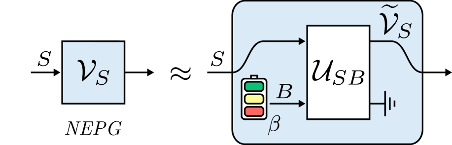
Figure 1: A non-energy-preserving gate (NEPG) $\mathcal{V}_{S}$ on the system $S$ can be approximated with a channel $\widetilde{\mathcal{V}}_{S}$, realized via a joint total-energy-preserving unitary transformation $\mathcal{U}_{SB}$ on the system and a battery $B$. To be useful for the task the initial state of the battery $\beta_{B}$ must present some coherence. We relate its entropic coherence $C(\beta_{B},H_{B})$ in Eq. (3), to the error in gate approximation, quantified by the worst-case infidelity $\epsilon_{wc}(\mathcal{V}_{S},\widetilde{\mathcal{V}}_{S})$ in Eq. (2).

In this framework the possible transformations induced on $S$ are given by the following family of CPTP maps [22]

$${\tt TEP}(H_{B},\beta_{B}):=\Big\{\widetilde{\mathcal{V}}_{S}({\rho}_{S})=\tr_{B}\mathcal{U}_{SB}[{\rho}_{S}\otimes\beta_{B}],$$

$$\qquad\qquad\qquad\qquad\text{s.t.}\;[{U}_{SB},{H}_{SB}]=0\Big\},$$ (1)

depending on the initial state of the battery ${\beta}_{B}$ and its Hamiltonian $H_{B}$. For ease of notation we also introduced $\mathcal{U}_{SB}[\bullet]:={U}_{SB}\bullet{U}^{{\dagger}}_{SB}$. Since our desire is to implement a fixed target map $\mathcal{V}_{S}$, we look for choices of ${\beta_{B}},H_{B}$ granting the best possible approximation thereof $\widetilde{\mathcal{V}}_{S}\approx\mathcal{V}_{S}$. This requirement can be put on formal grounds by minimizing a divergence between the maps, here the worst-case infidelity

$$\epsilon_{wc}(\mathcal{X}_{S},\mathcal{Y}_{S})=1-\min_{\rho_{SA}}F(\mathcal{X}_{S}[\rho_{SA}],\mathcal{Y}_{S}[\rho_{SA}])$$ (2)

where $F(\rho,\sigma)=\left(\tr|\sqrt{\rho}\sqrt{\sigma}|\right)^{2}$ and $A$ is any auxiliary system (some useful properties of $\epsilon_{wc}$ are summarized in App. A).

There are some conditions that the initial state of the battery should necessarily satisfy for high precision to be possible, often stated in terms of no-go theorems linking $\epsilon_{wc}$ with a certain amount of quantum resources [10] initially present in the battery . Different notions of resources $R(\beta_{B},H_{B})$, determined by battery Hamiltonian $H_{B}$ and its state ${\beta}_{B}$, have emerged in this context [16, 24, 13, 18]. We are specifically interested in its entropic coherence which we now define.

Entropic coherence as a resource for gate implementation.— For a system $B$ and with the Hamiltonian $H_{B}$, let $\mathcal{G}_{H_{B}}$ be the twirling map $\mathcal{G}_{H_{B}}[\bullet]:=\sum_{E}\Pi_{E}\bullet\Pi_{E}$, with $\Pi_{E}$ running through projectors on the eigenspaces of $H_{B}$. To a state $\rho_{S}$ of the system we associate the entropic coherence of energy, given by the following quantity

$$C(\rho_{B},H_{B})=S\big(\mathcal{G}_{H_{B}}[\rho_{B}]\big)-S\big(\rho_{B}\big),$$ (3)

where $S$ is the von Neumann entropy. Here we focus on energy for convenience, but the definition immediately generalizes to the entropic coherence of any additive quantity associated to an Hermitian operator. For a single system, $C(\rho_{B},H_{B})$ is identical to the relative entropy of superposition [18], computed with respect to energy eigenspaces of $H_{B}$. Furthermore, when $H_{B}$ is non-degenerate it also coincides with the relative entropy of coherence [19], computed with respect to the eigenbasis of $H_{B}$. However, in both cases a crucial difference appears when considering composite systems. In our case, the entropic coherence $C(H_{SB},\rho_{SB})$ of a joint state of two systems $S$ and $B$ is computed by applying Eq. (3) to the total Hamiltonian $H_{SB}=H_{S}+H_{B}$. In contrast, to compute the joint relative entropy of superposition/coherence one apples the same equation but for the composed twirling map $\mathcal{G}_{H_{S}}\otimes\mathcal{G}_{H_{B}}$ [18, 19], which leads to a very different class of free operations as we discuss below.

We show in App. B that EC satisfies the following four conditions, that we identify as prerequisites for any resource for the gate implementation task:

• It is non-increasing under energy preserving operations: $[U_{B},{H}_{B}]=0\implies C(\beta_{B},H_{B})=C(\mathcal{U}_{B}[\rho_{B}],H_{B})$;

• It is non-increasing under partial trace: $C(\rho_{BA},H_{BA})\geq C(\rho_{B},H_{B})$, where $A$ is an auxiliary system possibly correlated with $B$, and $\rho_{B}=\tr_{A}\rho_{BA}$;

• It is sub-additive on product states $C(\rho_{B}\otimes\rho_{A},H_{BA})\leq C(\rho_{B},H_{B})+C(\rho_{A},H_{A})$;

• It is regular with respect to the trace distance $D$, that is $\underset{D(\rho_{B},\sigma_{B})\rightarrow 0}{\lim}|C(\rho_{B},H_{B})-C(\sigma_{B},H_{B})|=0$.

The conditions closely resemble those proposed in [13, 25]. The crucial difference is that in (C1) we explicitly define the energy preserving operations as the set of free operations. This rules out the relative entropy of coherence as a valid resource, since for composite systems the latter can increase under generic energy preserving operations and is non-increasing only under a smaller set of unitary operations, which can not exchange energy between the subsystems. Namely, those of the form $U_{AB}=\bigoplus_{a,b}e^{i\varphi_{a,b}}U_{A}^{(E_{a})}\otimes U_{B}^{(E_{b})}$, with $U_{A}^{(E_{a})}$ and $U_{B}^{(E_{b})}$ operating on fixed energy subspaces for both subsystems. This implies that the bound on the relative entropy of coherence discussed in  [13, 25] is not relevant for the gate implementation task (see App. C for details).

Batteries suitable for the task.— We are interested in approximating a NEPG $\mathcal{V}_{S}$ on a quantum system with Hamiltonian $H_{S}$ and dimension $d_{S}$, by a channel $\widetilde{\mathcal{V}}_{S}\in{\tt TEP}(H_{B},\beta_{B})$ induced by a total-energy preserving operation on the system and the battery (see Eq. 1). In order to discuss the convergence of such channels to the ideal gate, we introduce the following definition.

Definition 1.

A family of batteries $\{H_{B}^{(\epsilon)},\beta_{B}^{(\epsilon)}\}_{\epsilon\in(0,\eta)}$ is called suitable for $\mathcal{V}_{S}$ if for every $\epsilon\in(0,\eta)$ there exist a channel

$$\widetilde{\mathcal{V}}_{S}\in{\tt TEP}(H_{B}^{(\epsilon)},\beta_{B}^{(\epsilon)})\quad\text{such that}\quad\epsilon_{wc}(\widetilde{\mathcal{V}}_{S},\mathcal{V}_{S})\leq\epsilon.$$ (4)

In words, $H_{B}^{(\epsilon)}$ and $\beta_{B}^{(\epsilon)}$ define a battery system capable of implementing $\mathcal{V}_{S}$ with $\epsilon$ precision, as quantified by the worst case fidelity in Eq. (2). This definition is general and, in particular, makes no assumptions on the size of the battery system and its scaling with $\epsilon$. However, as we will see, the final result can be significantly strengthened by introducing a mild assumption on the number of energy levels on which the battery state is supported. To do so let

$$\mathcal{N}(E,H_{B}):=\underset{E^{\prime}\leq E}{\sum}\text{Rank}[\Pi_{E^{\prime}}]$$ (5)

be the dimension of the subspace with energy bounded by $E$ for the battery system. Consider the following definition of a proportionate family of batteries, which has the number of accessible levels scaling at most polynomially with $\epsilon^{-1}$:

Definition 2.

A family of batteries $\{H_{B}^{(\epsilon)},\beta_{B}^{(\epsilon)}\}_{\epsilon\in(0,\eta)}$ is called proportionate if

$$\mathcal{N}(2E_{max}(\beta^{(\epsilon)}_{B}),H_{B}^{(\epsilon)})\leq\rm{poly}\left(\epsilon^{-1}\right),$$ (6)

where $E_{max}(\beta_{B}^{(\epsilon)}):=\max\{E\in\mathcal{E}[H_{B}^{(\epsilon)}]:\bra{E}\beta_{B}^{(\epsilon)}\ket{E}>0\}$ is the maximal energy on which the state $\beta_{B}^{(\epsilon)}$ is supported, and $\mathcal{E}[H]$ is the set of eigenvalues of $H$.

Entropic coherence is necessary for NEPG implementation.— With these definitions we are ready to state our main result, establishing a strong constraint on the entropic coherence of any battery system suitable to approximate the ideal gate.

Main Result (EC required to approximate a NEPG).

(i) If $\{H_{B}^{(\epsilon)},\beta_{B}^{(\epsilon)}\}_{\epsilon}$ is a suitable batteries family for the gate $\mathcal{V}_{S}$, then

$$C(\beta_{B}^{(\epsilon)},H_{B}^{(\epsilon)})\geq\frac{r_{2}(V_{S})}{8}\log(\frac{\sigma(V_{S})}{\epsilon})-o(1).$$ (7)

(ii) If $\{H_{B}^{(\epsilon)},\beta_{B}^{(\epsilon)}\}_{\epsilon}$ is also proportionate, then a stronger bound holds

$$C(\beta_{B}^{(\epsilon)},H_{B}^{(\epsilon)})\geq\frac{r_{2}(V_{S})}{4}\log(\frac{\sigma^{\prime}(V_{S})}{\epsilon\log^{2}(\epsilon^{-1})})-o(1).$$ (8)

Where $r_{2}(V_{S}),\sigma(V_{S}),\sigma^{\prime}(V_{S})$ only depend on the gate and the spectrum of $H_{S}$, $r_{2}(V_{S})\in\{1,..d_{S}^{2}-1\}$, and $\sigma(V_{S}),\sigma^{\prime}(V_{S})\geq 0$ with equality iff $[V_{S},H_{S}]=0$.

(iii) For a qubit system, with $p:=|\bra{0}V_{S}\ket{1}|^{2}$,

the above bound holds with $r_{2}(V_{S})=2$ , $\log(\sigma(V_{S}))=4\log(p)+{\it cst}$ and $\sigma^{\prime}(V_{S})=2\log(p)+{\it cst}$.

Here, $o(1)\to 0$ in the limit $\epsilon\to 0$, $r_{2}(V_{S})$, defined in Def. 12 in App. D.2, is connected to the incommensurability rank of the system’s energy spectrum $\mathcal{E}[H_{S}]$ [27], and $\sigma(V_{S}),\sigma^{\prime}(V_{S})>0$, defined in Eqs. (139,147), quantify the amount of asymmetry of $V_{S}$ with respect to $H_{S}$.

The result relies on the facts that $S$ has finite dimension $d_{S}$ and $\mathcal{V}_{S}$ unitary. Furthermore, the bounds depend on the gate $\mathcal{V}_{S}$ and the spectrum of the system Hamiltonian $H_{S}$. In App. D.2 we prove that if $H_{S},V_{S}$ are sampled randomly , then $r_{2}(V_{S})\geq d_{S}-1$ with probability 1.

Proof sketch of the main result.— Inspired by ref. [13], we consider $2m$ copies $S_{i}A_{i}$ of the system $SA$ with total Hamiltonian $H_{\bm{S}\bm{A}}=\underset{i=1}{\overset{2m}{\sum}}H_{S_{i}}+H_{A_{i}}$. The introduced auxiliary systems $A_{i}$ are copies of $S$ and never interact with the battery, their role will be clarified later. By hypothesis, there exists a TEP channel $\tilde{\mathcal{V}}_{S}(\cdot):=tr[\mathcal{U}_{SB}(\cdot\otimes\beta_{B})]$ such that $\epsilon_{wc}(\mathcal{V}_{S},\tilde{\mathcal{V}}_{S})\leq\epsilon$. Let the $S_{i}$ systems sequentially interact with a single battery $B$ in state $\beta_{B}$ via $~\mathcal{U}_{S_{i}B}$ (for odd $i$) and the adjoint unitary $\mathcal{U}^{*}_{S_{i}B}$ (for even $i$). Since the battery-systems interaction is energy preserving, and the EC satisfies (C1) and (C3), the extra entropic coherence in $\bm{SA}$ must be provided by the battery, formally for any initial state $\rho_{\bm{S}\bm{A}}=\rho_{SA}^{\otimes 2m}$, we have

$$C(\beta_{B},H_{B}) \geq C\big(\widetilde{\nu}_{\bm{S}\bm{A}},H_{\bm{S}\bm{A}}\big)-C\big(\nu_{\bm{S}\bm{A}},H_{\bm{S}\bm{A}}\big)$$

$$+C\big(\nu_{\bm{S}\bm{A}},H_{\bm{S}\bm{A}}\big)-C\big(\rho_{\bm{S}\bm{A}},H_{\bm{S}\bm{A}}\big),$$ (9)

where $\nu_{\bm{S}\bm{A}}=\big((\mathcal{V}_{S}\otimes\mathcal{V}^{*}_{S})^{\otimes m}\otimes\text{id}_{\bm{A}}\big)[\rho_{\bm{S}\bm{A}}]$ is the “ideal” final state, and $\widetilde{\nu}_{\bm{S}\bm{A}}$ (resulting from the action of $\mathcal{U}_{S_{i}B}$ and $\mathcal{U}^{*}_{S_{i}B}$) is guaranteed to be close to the latter $D(\widetilde{\nu}_{\bm{S}\bm{A}},\nu_{\bm{S}\bm{A}})\leq 4m\sqrt{\epsilon}$ [13].

Combing this inequality for $D(\widetilde{\nu}_{\bm{S}\bm{A}},\nu_{\bm{S}\bm{A}})$ with a refinement of property (C4), based on entropy continuity [28, 29], we bound the first line in Eq. (9)

$$C\big( \nu_{\bm{S}\bm{A}},H_{\bm{S}\bm{A}}\big)-C\big(\widetilde{\nu}_{\bm{S}\bm{A}},H_{\bm{S}\bm{A}}\big)\leq$$

$$16m^{2}\sqrt{\epsilon}(d_{S}-1)\log\left(d_{S}\right)+2\,h_{2}(4m\sqrt{\epsilon})-o(1),$$ (10)

where $h_{2}$ is the binary entropy. For proportionate batteries this inequality can be straightened to a linear function of $m$, which explains the difference between the two claims of the main result.

To bound the second line in Eq. (9), we chose $\rho_{\bm{S}\bm{A}}$ to be pure and eigenstate of $H_{\bm{S}\bm{A}}$, such that $C\big(\rho_{\bm{S}\bm{A}},H_{\bm{S}\bm{A}}\big)=0$. Then, we identify the quantity $C\big(\nu_{\bm{S}\bm{A}},H_{\bm{S}\bm{A}}\big)$ with the entropy of a sum of $2m$ i.i.d. discrete random variables. A lower bound on this entropy has recently been derived in  [27], and implies the following bound

$$C\big(\nu_{\bm{S}\bm{A}}, H_{\bm{S}\bm{A}}\big)-C\big(\rho_{\bm{S}\bm{A}},H_{\bm{S}\bm{A}}\big)\geq$$

$$\frac{r_{2}(V_{S})}{2}\log\big(2\pi e\;m\;g(V_{S})\big.)-o(1),$$ (11)

where $g(V_{S})$ quantifies the asymmetry of the gate and enters in both $\sigma(V_{S})$ and $\sigma^{\prime}(V_{S})$ later.

For a qubit system we proceed differently and bound Eq. (9) with an explicit construction of the initial state $\rho_{\bm{S}\bm{A}}$ which is not a product of $2m$ identical states. This yields a tighter but less general bound.

The last step is to combine the ineqs. (11) with (10) (or a stronger version for proportionate families and/or qubit gates) to bound the entropic coherence of the battery $C(\beta_{B},H_{B})$ via Eq. (9). Optimizing over the number of copies $m$ gives the final bounds $\square.$

Now, we discuss some implications of the result.
Vanishing error requires unbounded battery. – The first corollary, given below, is that any finite-dimensional battery is bound to a certain minimal implementation error. To the best of our knowledge, this is the first demonstration of this important physical insight. Additionally, it proves that for a qubit the NEPG implementation scheme with $O(\epsilon^{-\frac{1}{2}})$ battery levels, presented in [30], is tight in the exponent.

Corollary 3 (Vanishing error requires unbounded battery).

Let $\{H_{B}^{(\epsilon)},\beta_{B}^{(\epsilon)}\}_{\epsilon}$ be a suitable batteries family for the NEPG $\mathcal{V}_{S}$, then

$${\rm dim}[H_{B}^{(\epsilon)}]\geq\left(\frac{1-o(1)}{\log(\epsilon^{-1})}\right)^{\frac{r_{2}(V_{S})}{2}}\left(\frac{\sigma^{\prime}(V_{S})}{\epsilon}\right)^{\frac{r_{2}(V_{S})}{4}}\to\infty$$ (12)

in the limit $\epsilon\to 0$.

Proof.

If $\{H_{B}^{(\epsilon)},\beta_{B}^{(\epsilon)}\}_{\epsilon}$ is not proportionate, ${\rm dim}[H_{B}^{(\epsilon)}]$ must grow exponentially with $\epsilon^{-1}$ and the bound is true. Otherwise, we obtain the corollary by combining Eq. (7) with the following immediate upper bound on the coherent entropy of energy $C(\beta_{B}^{(\epsilon)},H_{B}^{(\epsilon)})\leq 2^{{\rm dim}[H_{B}^{(\epsilon)}]}$ implied by the dimension of the state. ∎

Implications for other resources.— Without any assumption on the Hamiltonian of the system the entropic coherence gives no informations on the content of other quantities studied for our task, like energy or quantum Fisher information. However, as we now demonstrate, once the spectrum of $H_{B}$ is fixed, the presence of entropic coherence in the battery implies strong bound on the presence of other resources.

In particular, we show in App. E that for any system with $C(\beta_{B},H_{B})\geq C$, the average energy satisfy

$$\tr(H_{B}\beta_{B}) \geq\frac{\tr(H_{B}e^{-\gamma_{C}H_{B}})}{\tr(e^{-\gamma_{C}H_{B}})}$$ (13)

where the Lagrangian multiplier $\gamma_{C}$ is determined by the equation $S\left(\frac{e^{-\gamma_{C}H_{B}}}{\tr e^{-\gamma_{C}H_{B}}}\right)=C$ .

Once the spectrum of $H_{B}$ is fixed the rhs of Eqs. (13) can be easily computed. For illustration, we now consider the example of an harmonic oscillator. In this case Eq. (13) implies $\tr[\beta_{B}H_{B}]\geq\omega\,(2^{C(\beta,H_{B})-1}-1)+o(1)$ in the large $C(\beta_{B},H_{B})$ limit. In fact, for any system whose spectral volume grows linearly with the energy

$$\mathcal{N}(H_{B}^{(\epsilon)},E)\leq 1+\eta E,$$ (14)

this simple argument implies the following corollary of the main result (see App. E for derivation).

Corollary 4 (Energy constraint to implement NEPGs).

Let $\{H_{B}^{(\epsilon)},\beta_{B}^{(\epsilon)}\}_{\epsilon}$ be suitable for the NEPG $\mathcal{V}_{S}$, and $\mathcal{N}(H_{B}^{(\epsilon)},E)\leq 1+\eta E$ then

$$\tr[\beta_{B}^{(\epsilon)}H_{B}^{(\epsilon)}]\geq\left[\frac{\sigma(V_{S},H_{S})}{2\eta}+o(1)\right]\epsilon^{-\frac{r_{2}(V_{S},H_{S})}{8}}.$$ (15)

This corollary is particularly remarkable for systems and gates that operate on non-harmonic energy levels, i.e. such that $r_{2}(V_{S},H_{S})>2$ (or $r_{2}(V_{S},H_{S})>4$ for a non-proportionate battery). In this case the bound (15) is stronger in the scaling than all previously known results [13, 30].

We leave open the question whether the extra energy cost required by corollary 4 can be avoided with a battery not satisfying the spectral volume constraint (14). Nevertheless, we speculate that for $r_{2}(V_{S},H_{S})\geq 2$, a more energy efficient battery system would be composed of multiple harmonic oscillators with frequencies resonant with each transition.

A similar argument holds for the variance and its convex roof, i.e. the Quantum Fischer Information (QFI) [32]. In App. E we prove the following

Corollary 5 (QFI constraits to implement NEPGs).

Let $H_{B}$ be a harmonic oscillator of frequency $\omega$ and $\{H_{B},\beta_{B}^{(\epsilon)}\}_{\epsilon}$ be suitable for the NEPG $\mathcal{V}_{S}$, then

$${\rm QFI}(\beta,H_{B})\geq\left(\frac{\omega^{2}\sigma(V_{S},H_{S})^{2}}{e\pi}+o(1)\right)(\epsilon d_{S})^{-\frac{r_{2}(V_{S},H_{S})}{4}}.$$ (16)

We believe that this result can be generalized up to a constant to all batteries whose energies do not concentrate $\mathcal{N}(E+\omega,H_{B})-\mathcal{N}(E,H_{B})\leq\eta\omega$. In [16], it was shown that there always exist batteries $\{\beta^{\epsilon},H_{B}^{\epsilon}\}$ suitable for $V_{S}$ with ${\rm QFI}(\beta,H_{B})\simeq\epsilon^{-1}$. Thus, the corollary demonstrates that for systems with $r_{2}(V_{S},H_{S})>2$ (or $r_{2}(V_{S},H_{S})>4$ in the non-proportionate case) harmonic oscillators make very sub-optimal batteries.

Conclusions.—

We investigated the role of entropic coherence of energy as a fundamental resource for the implementation of non-energy-preserving gates (NEPGs). We established that, to implement any NEPG with accuracy $\epsilon$, a minimum amount of entropic coherence scaling as $r\log(\epsilon^{-1})$ is required in the battery, where $r\geq 1/8$ depends on the specific system and gate. Under mild assumptions on the battery, this bound is strengthened by a factor of two and is tight in the case of qubits.

We then examine the implications of this bound. First, we show that the dimension of the battery system must scale at least as $d_{B}\sim\epsilon^{-\frac{r}{4}}$, thus diverging to enable perfect implementation. Furthermore, we demonstrated that the battery’s energy and Quantum Fisher Information (QFI) must scale similarly, provided the Hamiltonian has a bounded density of energy levels. These bounds can be stricter than those derived independently in [13, 16], suggesting a hierarchy among physical resources. Notably, constraints on energy and QFI do not imply corresponding limits on EC, since, by rescaling the battery’s Hamiltonian, both energy and QFI can become arbitrarily large while EC remains unchanged. Finally, our results offer criteria for evaluating the efficiency of batteries in implementing NEPGs. In particular, for systems with multiple incommensurable energy gaps, batteries with a bounded energy level density are shown to be highly inefficient. We speculate that a battery composed of multiple harmonic oscillators—one for each energy gap—could instead prove to be efficient.

Future developments could aim to tighten the inequality by a factor of two for arbitrary systems, by extending the strategy used in the qubit case, namely selecting an appropriately entangled initial state during the resource production stage of the proof. Another promising direction is to derive upper bounds on the EC cost by explicitly constructing battery states and interactions that implement non-energy-preserving gates beyond the already explored case of equally spaced energy levels [33, 13, 30].

Acknowledgments :– RC and PS acknowledge support from Swiss National Science Foundation (NCCR SwissMAP). VC and VG acknowledge financial support by MUR (Ministero dell’ Università e della Ricerca) through the PNRR MUR project PE0000023-NQSTI. M.P.-L. acknowledges support from the Grant RYC2022-036958-I funded by MICIU/AEI/10.13039/501100011033 and by ESF+.

Appendix A Channel distances and their relationships

To evaluate how successful the setup in Fig. 1 was we need a way to measure how much the maps $\widetilde{\mathcal{V}}_{S}\in{\tt TEP}(H_{B},\beta_{B})$ and $\mathcal{V}_{S}$ are close the one to the other. This can be done by using several channel distances between two quantum channels $\mathcal{E}_{1}$ and $\mathcal{E}_{2}$ acting on the system $X$. A commonly used distance is the diamond norm

$$\lVert\mathcal{E}_{1}-\mathcal{E}_{2}\rVert_{\diamond}:=\underset{\rho_{SA}\in\mathcal{D}(\mathcal{H}_{SA})}{\text{sup}}D\Big((\mathcal{E}_{1}\otimes\text{id}_{A})[{\rho}_{SA}],(\mathcal{E}_{2}\otimes\text{id}_{A})[{\rho}_{SA}]\Big),$$ (17)

where the channels are trivially extended to act on an auxiliary system $A$ (that can be taken of the same dimension as $X$ without loss of generality), the supremum is taken over all states $\rho_{XA}$ of the composed systems $XA$, and $D(\rho,\sigma)=\frac{1}{2}\tr|\rho-\sigma|$ is the trace distance. The diamond norm has the operational meaning of the best single-shot distinguishability between the two channels.

Similarly, the notion of fidelity between quantum states can be generalized to channels by introducing the worst-case fidelity

$$F_{wc}(\mathcal{E}_{1},\mathcal{E}_{2}):=\underset{\rho_{SA}\in\mathcal{D}(\mathcal{H}_{SA})}{\text{inf}}F\Big((\mathcal{E}_{1}\otimes\text{id}_{A})[{\rho}_{SA}],(\mathcal{E}_{2}\otimes\text{id}_{A})[{\rho}_{SA}]\Big),$$ (18)

where use the definition of fidelity with the square $F(\rho,\sigma)=\left(\tr|\sqrt{\rho}\sqrt{\sigma}|\right)^{2}$. Using $F_{wc}$ we can define the worst-case infidelity

$$\epsilon_{wc}(\mathcal{E}_{1},\mathcal{E}_{2}):=1-F_{wc}(\mathcal{E}_{1},\mathcal{E}_{2}).$$ (19)

Notice that $\epsilon_{wc}(\mathcal{E}_{1},\mathcal{E}_{2})$ is not a distance because it fails to satisfy the triangle inequality, however one can verify that the worst-case angle $A_{wc}(\mathcal{E}_{1},\mathcal{E}_{2}):=\arccos(\sqrt{F_{wc}(\mathcal{E}_{1},\mathcal{E}_{2})})$ is instead a distance. The worst-case infidelity is the error quantifier used in our definition of the gate approximation task. It is related to the diamond norm by the following inequalities

$$1-\sqrt{1-\epsilon_{wc}(\mathcal{E}_{1},\mathcal{E}_{2})}\leq\lVert\mathcal{E}_{1}-\mathcal{E}_{2}\rVert_{\diamond}\leq\sqrt{\epsilon_{wc}(\mathcal{E}_{1},\mathcal{E}_{2})},$$ (20)

which is a direct consequence of the Fuchs Van-der Graaf inequality $1-\sqrt{F({\rho},{\tau})}\leq D({\rho},{\tau})\leq\sqrt{1-F({\rho},{\tau})}$ [34].

Appendix B The entropic coherence is a resource for the gate implementation

We start by introducing the set of incoherent states. Let $A,B$ be two system with respective Hamiltonians $H_{A},H_{B}$, the incoherent states are defined as

$$\Delta_{AB} :=\{{\rho}_{AB}:C({\rho}_{AB},{H}_{A}+{H}_{B})=0\};$$ (21)

$$\Delta_{B} :=\{{\rho}_{B}:C({\rho}_{B},{H}_{B})=0\}.$$

It is immediate to verify that every incoherent state of a given Hamiltonian $H$ is a fixed point of the corresponding twirling channel $\mathcal{G}_{H}$ i.e., if $\rho\in\Delta$ then $\mathcal{G}_{H}(\rho)=\rho$, and that $\mathcal{G}_{H}(\sigma)\in\Delta\quad\forall\sigma\in\mathcal{D}[\mathcal{H}]$, making it a projector into the incoherent states set. It is also evident that $\rho$ is an incoherent states if and only if it does not evolve under the action of $e^{-iHt}$, i.e. $\rho\in\Delta\Longleftrightarrow\rho=e^{-iHt}\rho e^{iHt}$ for all $t$. Further, jointly incoherent states are locally incoherent:

Lemma 6.

Let $\Delta_{AB}$, $\Delta_{B}$ be the sets of incoherent states as (21), then $Tr_{A}[\Delta_{BA}]=\Delta_{B}$.

Proof.

The inclusion $Tr_{A}[\Delta_{AB}]\supseteq\Delta_{B}$ is trivial. On the other hand given $\rho_{AB}\in\Delta_{AB}$ we have that for all $t$ it holds $\rho_{AB}=e^{-it(H_{A}+H_{B})}\rho_{AB}e^{+it(H_{A}+H_{B})}$. Taking the partial trace over $A$ on both sides we have $\rho_{B}=Tr_{A}[e^{-it(H_{A}+H_{B})}\rho_{AB}e^{+it(H_{A}+H_{B})}]=e^{-itH_{B}}\rho_{B}e^{-itH_{B}}$, proving that $\Delta_{B}\supseteq Tr_{A}[\Delta_{AB}]$ and so the thesis. ∎

We now prove that the entropic coherence admits other tree equivalent definitions:

$$(i)\quad C(\rho,H):=S(\mathcal{G}_{H}(\rho))-S(\rho),$$ (22)

$$(ii)\quad C(\rho,H)=S(\rho||\mathcal{G}_{H}(\rho)),$$ (23)

$$(iii)\quad C(\rho,H)=\underset{\sigma\in\Delta}{\min}S(\rho||\sigma).$$ (24)

Proof.

We use the identity $\log(\sigma)=\log(\mathcal{G}_{H}(\sigma))=\mathcal{G}_{H}(\log(\sigma))$, and the fact that $\mathcal{G}_{H}$ is self adjoint, to prove

$$S(\rho||\sigma)=-Tr[\rho\log(\sigma)]-S(\rho)=-Tr[\rho\mathcal{G}_{H}(\log(\sigma))]-S(\rho)$$

$$=Tr[\mathcal{G}_{H}(\rho)\log(\sigma)]-S(\rho)=S(\mathcal{G}_{H}(\rho))-S(\rho)+S(\mathcal{G}_{H}(\rho)||\sigma).$$ (25)

This equality proves $(i)\iff(ii)$ since for $\sigma=G_{H}(\rho)$ one has $S(G_{H}(\rho)||\sigma)=0$, and $(i)\iff(iii)$ because for all other choices of $\sigma$ one has $S(G_{H}(\rho)||\sigma)>0$. ∎

Notice that in particular the expression $(iii)$ makes it explicit that the Entropic Coherence can be seen as the relative entropy of resource, where $\Delta$ is the convex set of free states. This guarantees that (EC) satisfies many desired properties as a coherence quantifier [21, 35]. We now prove that it additionally satisfies $C_{1}-C_{4}$ of the main text:

Proof.

First, since $\mathcal{G}_{H}$ is unital channel, $C_{r}(\rho,H)\geq 0$ [36].
(C1) If $[U,H]=0$ then $\mathcal{G}_{H}\circ\mathcal{U}=\mathcal{U}\circ\mathcal{G}_{H}$ thus

$$C(\mathcal{U}(\rho),H)=S(\mathcal{G}_{H}\circ\mathcal{U}(\rho))-S(\mathcal{U}(\rho))$$ (26)

$$=S(\mathcal{G}_{H}(\rho))-S(\rho)=C(\rho,H).$$ (27)

(C2) From lemma 6 we know that $\Delta_{A}=tr_{B}[\Delta_{AB}]$, thus we have

$$C(\rho_{AB},H_{AB})=\underset{\sigma\in\Delta_{AB}}{\min}S(\rho_{AB}||\sigma)\geq\underset{\sigma\in\Delta_{AB}}{\min}S(\rho_{A}||tr_{B}[\sigma])$$ (28)

$$=\underset{\sigma\in\Delta_{A}}{\min}S(\rho_{A}||\sigma):=C(\rho_{A},H_{A})$$ (29)

where in the first inequality we used the data processing inequality of the relative entropy [37] $S(\mathbf{\Phi}(\rho)||\mathbf{\Phi}(\sigma))\leq S(\rho||\sigma)$.

(C3) First observe that $\Delta_{A}\otimes\Delta_{B}\subseteq\Delta_{AB}$ i.e. the tensor product of incoherent states is still incoherent with the respect to the joint system, this implies according to caracterization (iii)

$$S(\rho_{A}\otimes\sigma_{B}||\mathcal{G}_{H_{AB}}(\rho_{A}\otimes\sigma_{B}))\leq S(\rho_{A}\otimes\sigma_{B}||\mathcal{G}_{H_{A}}(\rho_{A})\otimes\mathcal{G}_{H_{B}}(\sigma_{B}))$$ (30)

$$=S(\rho_{A}||\mathcal{G}_{H_{A}}(\rho_{A}))+S(\sigma_{B}||\mathcal{G}_{H_{B}}(\sigma_{B})).$$ (31)

(C4) Because the twirled states are closer in trace distance than their counterparts, we can apply the Fannes-Audenaert inequality [38] twice:

$$\absolutevalue{C(\rho,H)-C(\sigma,H)}\leq\absolutevalue{S(\overline{\rho})-S(\overline{\sigma})}+\absolutevalue{S(\rho)-S(\sigma)}$$ (32)

$$\leq 2\log(d-1)D(\rho,\sigma)+2h_{2}(D(\rho,\sigma)),$$ (33)

where $d:=dim(\mathcal{H})$ and $h_{2}(x):=-x\log(x)-(1-x)\log(1-x)$ is the binary entropy. ∎

Appendix C Comment on the bound on the relative entropy of coherence in refs [13, 25]

In [13, 25] a theorem analogous to our result was derived for a similarly looking quantity, the relative entropy of coherence (REC). However, in these works the definition of REC differs for ours in a subtle way that turns out to be dramatically less relevant in this context of NEPG implementation, as we now explain.

Let $S,B$ be two quantum systems with respective Hamiltonians $H_{S},H_{B}$. Let $\mathcal{G}_{{H}_{S}},\mathcal{G}_{{H}_{B}}$ be the respecting dephasing channels. Accordingly to the definition used in refs. [13, 25], the REC of a composite system, that we denote $C_{loc}(\cdot)$, reads

$$C_{loc}(\rho_{SB}):=S(\mathcal{G}_{{H}_{S}}\circ\mathcal{G}_{{H}_{B}}(\rho_{SB}))-S(\rho_{SB}).$$ (34)

Notice that in this definition the knowledge of the total Hamiltonian $H_{SB}$ and the joint state $\rho_{SB}$ does not uniquely specify the value of $C_{loc}(\rho_{SB})$, instead the partition of the global system in subsystems must be specified. Furthermore, in refs. [13, 25] our condition C1 is replaced with the request that a resource should be non-increasing under free operations and partial trace, while free operations are defined as being not able to increase resources. From the latter we conclude that

$$U_{SB}\quad\textit{is a free unitary}\quad\iff U_{SB}\ket{E_{a}}_{S}\otimes\ket{E_{b}}_{B}=e^{i\phi_{E_{a},E_{b}}}\ket{E_{a}}_{S}\otimes\ket{E_{b}}_{B},$$ (35)

for some arbitrary real phases $\{\phi_{E_{a},E_{b}}\}_{a,b}$, and denote with ${\tt LEP}(\beta_{B},H_{B})$ the set of operations induced by such free unitaries on the system $S$, analogously to Eq. (1). This set of operations is much more constrained than the set ${\tt TEP}(\beta_{B},H_{B})$, defined with the total energy preserving condition $[U_{SB},H_{S}+H_{B}]=0$. Crucially, it simply forbids interactions to exchange energy between systems $S$ and $B$, i.e.

for all $\widetilde{\mathcal{V}}_{S}\in{\tt LEP}(\beta_{B},H_{B})$ and $\rho_{S}$

$$\tr[H_{S}\widetilde{\mathcal{V}}_{S}(\rho_{S})]=\tr[H_{S}\rho_{S}].$$ (36)

In view of this it shouldn’t come as a surprise that the bound found in Eq.(10) of [13] is exponentially higher than ours

$$C_{loc}(\beta_{B},H_{B})\geq\frac{f(V_{S})}{\sqrt{\epsilon_{wc}}}-o(1).$$ (37)

As a matter of fact any NEPG $V_{S}$ cannot be approximated arbitrary well by channels in ${\tt LEP}(\beta_{B},H_{B})$ irrespectivly of the chosen $\beta_{B},H_{B}$. On the other hand Eq.(37) is only valid in the $\epsilon_{wc}\rightarrow 0$ limit, making the theorem inapplicable.

Appendix D Proof of the main result

This section is devoted to the proof of the main result on the main text.

D.1 Resource inequalities and proof outline

In this section we will present a generalization of the method used in [13, 25] and show how to use a resource satisfying the properties (C1)-(C4) to create a bound on the precision in the implementation of NEPGs. For this sake, let us consider a battery $B$ in contact with a system $S$ and an auxiliary system $A$ (this will be convenient later on). Let the joint system $SA$ be prepared in the state $\rho_{SA}$ and the battery in $\beta_{B}$, as usual. Further, we always suppose the energy to be additive, i.e. $H_{SBA}:=H_{S}+H_{B}+H_{A}$. We now prove the following lemma.

Lemma 7.

Consider a system with Hamiltonian $H_{S}$ and a battery with Hamiltonian $H_{B}$, prepared in the state $\beta_{B}$. Let $\mathcal{U}_{SB}[\bullet]=U_{SB}\bullet U_{SB}^{\dagger}$ be a joint unitary channel, commuting with the total hamiltonian $[U_{SB},H_{S}+H_{B}]=0$, and $\widetilde{\mathcal{V}}_{S}[\bullet]=\tr_{B}\mathcal{U}_{SB}[\bullet\otimes\beta_{B}]$ be the channel induced by this unitary on the system (element of ${\tt TEP}(H_{B},\beta_{B})$). Then, for any initial state $\rho_{SA}$ of the system S and and an auxiliary system $A$, with Hamiltonian $H_{A}$, the following bound holds

$$C\big(\beta_{B},H_{B}\big)\geq C\big(\widetilde{\mathcal{V}}_{S}[\rho_{SA}],H_{S}+H_{A}\big)-C\big(\rho_{SA},H_{S}+H_{A}\big).$$ (38)

Proof.

Using the properties (C3), (C1) we can write

$$C(\beta_{B},H_{B})+C(\rho_{SA},H_{SA})\geq C(\beta_{B}\otimes\rho_{SA},H_{SBA})=C\big((\mathcal{U}_{SB}\otimes\text{id}_{A})[\beta_{B}\otimes\rho_{SA}],H_{SBA}\big)$$ (39)

Using the definition of $\widetilde{\mathcal{V}}_{S}$ as the trace over $B$ of the global evolution and property (C2) we obtain

$$C\big((\mathcal{U}_{SB}\otimes\text{id}_{A})[\beta_{B}\otimes\rho_{SA}],H_{SBA}\big)\geq C(\widetilde{\mathcal{V}}_{S}\otimes\mathcal{I}_{A}(\rho_{AS}),H_{SA}).$$ (40)

∎

The general idea now is to somehow apply this bound to our channel of interest $\widetilde{\mathcal{V}}_{S}$ approximating $\mathcal{V}_{S}$. However, following [13] we note that a tighter result can be obtained when applying the bound to several copies of this channel. Therefore, we now consider $2m$ copies of the system $S$, labeled $S_{i}$ for $i\in\{1,...2m\}$, and denote their composite system with $\bm{S}=S_{1}\dots S_{2m}$. For any (single copy) total-energy-preserving unitary channel $\mathcal{U}_{SB}$, its adjoint $\mathcal{U}^{*}_{SB}[\bullet]=U_{SB}^{\dagger}\bullet U_{SB}$, and any state of the battery $\beta_{B}$ we define the following channels

$$\mathcal{U}^{(m)}_{\bm{S}B}:=\mathcal{U}_{S_{2m}B}^{*}\circ\mathcal{U}_{S_{2m-1}B}\circ...\circ\mathcal{U}_{S_{2}B}^{*}\circ\mathcal{U}_{S_{1}B}$$ (41)

$$\widetilde{\mathcal{V}}_{\bm{S}}^{(m)}[\bullet_{\bm{S}}]:=\tr_{B}\mathcal{U}^{(m)}_{\bm{S}B}[\bullet_{\bm{S}}\otimes\beta_{B}],$$ (42)

where $\mathcal{U}^{(m)}_{\bm{S}B}$ is a unitary channel on $\bm{S}B$,

and $\widetilde{\mathcal{V}}_{\bm{S}}^{(m)}$

is a CPTP map on $\bm{S}$. Similarly, let us define the target unitary channel on the $2m$ system copies

$$\mathcal{V}^{(m)}_{\bm{S}}:=\underset{i=1}{\overset{m}{\bigotimes}}\,\mathcal{V}_{S_{i}}\otimes\mathcal{V}_{S_{i+1}}^{*}.$$ (43)

Our choice for these specific definitions of the many copy maps $\mathcal{U}_{\bm{S}B}^{(m)}$ and $\mathcal{V}^{(m)}_{\bm{S}}$ in Eqs. (41-43) in motivated by the following theorem, relating their distance to the single-copy error $\epsilon_{wc}(\widetilde{\mathcal{V}}_{S};\mathcal{V}_{S})$.

Theorem 8.

[13] Consider the maps defined in Eqs. (41) and (43). For the following CPTP maps from $L(\mathcal{H}_{\bm{S}})\to L(\mathcal{H}_{\bm{S}}\otimes\mathcal{H}_{B})$, where $L(\mathcal{H})$ denotes the space of linear operators acting on the Hilbert space $\mathcal{H}$, we have

$$\lVert\mathcal{U}^{(m)}_{\bm{S}B}[\bullet_{\bm{S}}\otimes\beta_{B}]-\mathcal{V}^{(m)}_{\bm{S}}[\bullet_{\bm{S}}]\otimes\beta_{B}\rVert_{\diamond}\leq 4m\sqrt{\epsilon_{wc}(\widetilde{\mathcal{V}}_{S};\mathcal{V}_{S})}.$$ (44)

Thanks to this theorem and using the definition of diamond norm in Eq. (17) we have

$$D\left(\mathcal{U}^{(m)}_{\bm{S}B}[{\rho}^{(m)}_{\bm{S}\bm{A}}\otimes\beta_{B}],\mathcal{V}^{(m)}_{\bm{S}}[\rho^{(m)}_{\bm{S}\bm{A}}]\otimes\beta_{B}\right)\leq 4m\sqrt{\epsilon_{wc}(\widetilde{\mathcal{V}}_{S};\mathcal{V}_{S})},$$ (45)

that holds for any state $\rho^{(m)}_{\bm{S}\bm{A}}$ of the system $\bm{S}$ extended with any auxiliary system $\bm{A}$. Since the trace distance is non-increasing under partial trace, this inequality still holds when the battery is traced out

$$D\left(\widetilde{\mathcal{V}}_{\bm{S}}^{(m)}[\rho_{\bm{S}\bm{A}}^{(m)}],\mathcal{V}_{\bm{S}}^{(m)}[\rho_{\bm{S}\bm{A}}^{(m)}]\right)=D\left(\widetilde{\nu}_{\bm{S}\bm{A}}^{(m)},\nu_{\bm{S}\bm{A}}^{(m)}\right)\leq 4m\sqrt{\epsilon_{wc}(\widetilde{\mathcal{V}}_{S};\mathcal{V}_{S})}.$$ (46)

Here we introduced the states

$$\widetilde{\nu}_{\bm{S}\bm{A}}^{(m)}:=\widetilde{\mathcal{V}}_{\bm{S}}^{(m)}[\rho_{\bm{S}\bm{A}}^{(m)}]\qquad\text{and}\qquad\nu_{\bm{S}\bm{A}}^{(m)}:=\mathcal{V}_{\bm{S}}^{(m)}[\rho^{(m)}_{\bm{S}\bm{A}}],$$ (47)

which implicitly depend on $\rho^{(m)}_{\bm{S}\bm{A}}$ and are central for the following discussion.

In addition, note that the global unitary $\mathcal{U}_{\bm{S}B}^{(m)}$ manifestly commutes with the total Hamiltonian of the $2m$ systems and the battery $H_{\bm{S}}+H_{B}$, with $H_{\bm{S}}=\sum_{i=1}^{2m}H_{S_{i}}$. Hence, Lemma 7 immediately implies the following bound

$$C(\beta_{B},H_{B}) \geq C\big(\widetilde{\mathcal{V}}^{(m)}_{\bm{S}}[\rho^{(m)}_{\bm{S}\bm{A}}],H_{\bm{S}}+H_{\bm{A}}\big)-C\big(\rho^{(m)}_{\bm{S}\bm{A}},H_{\bm{S}}+H_{\bm{A}}\big)$$ (48)

$$=C\big(\nu_{\bm{S}\bm{A}}^{(m)},H_{\bm{S}}+H_{\bm{A}}\big)-C\big(\rho_{\bm{S}\bm{A}}^{(m)},H_{\bm{S}}+H_{\bm{A}}\big)$$ (49)

$$-\left(C\big(\nu_{\bm{S}\bm{A}}^{(m)},H_{\bm{S}}+H_{\bm{A}}\big)-C\big(\widetilde{\nu}_{\bm{S}\bm{A}}^{(m)},H_{\bm{S}}+H_{\bm{A}}\big)\right)$$ (50)

for any choice of auxiliary system $\bm{A}$ (Hilbert space $\mathcal{H}_{\bm{A}}$), its Hamiltonian $H_{\bm{A}}$ and the initial state $\rho_{\bm{S}\bm{A}}$. Clearly, we want to select them in a way to maximize the rhs in the above bound. With this in mind we decompose the rest of the proof in the following steps:

• We obtain a lower bound on the resource production

  $$C\big(\nu_{\bm{S}\bm{A}}^{(m)},H_{\bm{S}}+H_{\bm{A}}\big)-C\big(\rho_{\bm{S}\bm{A}}^{(m)},H_{\bm{S}}+H_{\bm{A}}\big)\geq(\ast)$$

  in Eq. (49), as a function of the properties of the ideal gate $\mathcal{V}_{S}$. A convenient choice is to restrict the analysis to initial states that are pure and eigenstates of the total Hamiltonian. In this way $C\big(\rho_{\bm{S}\bm{A}}^{(m)},H_{\bm{S}}+H_{\bm{A}}\big)=0$ and $C\big(\nu_{\bm{S}\bm{A}}^{(m)},H_{\bm{S}}+H_{\bm{A}}\big)$ is mapped into the entropy of a sum of i.i.d. random variables (see Lemma 10). Furthermore, the auxiliary systems are chosen to be copies of $S$, but with a flipped Hamiltonian $H_{A_{i}}=-H_{S}$.

• We obtain an upper bound on the resource regularity

  $$C\big(\nu_{\bm{S}\bm{A}}^{(m)},H_{\bm{S}}+H_{\bm{A}}\big)-C\big(\widetilde{\nu}_{\bm{S}\bm{A}}^{(m)},H_{\bm{S}}+H_{\bm{A}}\big)\leq(\ast\ast)$$

  in Eq. (50) as a function of the single-channel error $\epsilon_{wc}(\widetilde{\mathcal{V}}_{S};\mathcal{V}_{S})$. Here, the idea consists of bounding the term with the trace distance between the states $\nu_{\bm{S}\bm{A}}^{(m)}$ and $\widetilde{\nu}_{\bm{S}\bm{A}}^{(m)}$, and then applying the bound (44). For this purpose, we will use a refinement of the Fannes-Audenaert inequality (see Lemma 14) which holds in full generality. We then derive a specific bound for the choices of $H_{\bm{A}}$ and $\rho_{\bm{S}\bm{A}}^{(m)}$ used in step 1. We derive a general bound, and a refined one assuming that the battery is proportionate.

• We combine the two bounds obtained in steps 1 and 2, which still depend on the choice of the initial pure state $\rho^{(m)}_{\bm{S}\bm{A}}$. We then select this state so that the difference $(\ast)-(\ast\ast)\leq C(\beta{B},H_{B})$, which lower bounds our quantity of interest via Eq. (48), is provably large. Finally, we maximize the obtained bound with respect to the number of copies $m$.

The step 1 of the proof holds for any resource $C$ fulfilling properties (C1-C4). In contrast, in the following we explicitly consider the entropic coherence of energy.

D.2 Step 1: Bounding the resource production

Our goal here, is to choose specific initial states $\rho_{\bm{S}\bm{A}}^{(m)}$ that ‘nicely’ lower bounds the expression in Eq. (49), which corresponds to the amount of resource produced by the gate $\mathcal{V}_{\bm{S}}^{(m)}$ acting on the state. Using the definition of the entropic coherence we get

$$C\big(\nu_{\bm{S}\bm{A}}^{(m)},H_{\bm{S}}+H_{A}\big)-C\big(\rho_{\bm{S}\bm{A}}^{(m)},H_{\bm{S}}+H_{\bm{A}}\big)=S\left(\mathcal{G}_{H_{\bm{S}\bm{A}}}[\nu_{\bm{S}\bm{A}}^{(m)}]\right)-S(\nu_{\bm{S}\bm{A}}^{(m)})-S\left(\mathcal{G}_{H_{\bm{S}\bm{A}}}[\rho_{\bm{S}\bm{A}}^{(m)}]\right)+S(\rho_{\bm{S}\bm{A}}^{(m)}).$$ (51)

Since the states are assumed pure and eigenstates of the total Hamiltonian, we have $S\left(\rho_{\bm{S}\bm{A}}^{(m)}\right)=S\left(\nu_{\bm{S}\bm{A}}^{(m)}\right)=S\left(\mathcal{G}_{H_{\bm{S}\bm{A}}}[\rho_{\bm{S}\bm{A}}^{(m)}]=\rho_{\bm{S}\bm{A}}^{(m)}\right)=0.$ Hence, the ‘production of resource’ is equal to the only remaining term, i.e. the entropy of the final state after twirling

$$C\big(\nu_{\bm{S}\bm{A}}^{(m)},H_{\bm{S}}+H_{A}\big)-C\big(\rho_{\bm{S}\bm{A}}^{(m)},H_{\bm{S}}+H_{\bm{A}}\big)=S\left(\mathcal{G}_{H_{\bm{S}\bm{A}}}[\nu_{\bm{S}\bm{A}}^{(m)}]\right).$$ (52)

To lower bound the right hand side it is convenient to identify it with the entropy of a random variable, given by the following definition.

Definition 9.

Let $\psi=\outerproduct{\psi}{\psi}$ be a pure state of a $d$-dimensional quantum system, and $H=\underset{j=1}{\overset{k}{\sum}}E_{j}\Pi_{E_{j}}$ the associated Hamiltonian. We call $X_{\psi}$ the discrete random variable taking values in the set

$$\chi_{\psi}:=\{E_{j}\in\mathcal{E}(H):\bra{\psi}\Pi_{E_{j}}\ket{\psi}>0\},$$ (53)

and distributed accordingly to ${\rm Pr}(X_{\psi}=E_{j})=\bra{\psi}\Pi_{E_{j}}\ket{\psi}$, i.e. the random variable describing the outcome of an energy measurement on the state $\psi$. It is immediate to see that

$$S\left(\mathcal{G}_{H}[\psi]\right)=S(X_{\psi}).$$ (54)

The following lemma will also be useful.

Lemma 10.

Let $\Psi_{\bm{T}}$ be a pure state of systems $\bm{T}=T_{1}\dots T_{m}$, with associated Hamiltonians $H_{T_{i}}=\underset{j}{\sum}E_{i}^{(j)}\Pi_{T_{i}}^{(j)}$ and $H_{\bm{T}}=\underset{i=1}{\overset{m}{\sum}}H_{T_{i}}$. Then

$$S\left(\mathcal{G}_{H_{\bm{T}}}[\Psi_{\bm{T}}]\right)=S\left(\sum_{i=1}^{m}X_{\Psi}^{(i)}\right),$$ (55)

where the random variables $X_{\Psi}^{(i)}$ take the values in $\mathcal{E}(H_{T_{i}})$ and are distributed accordingly to ${\rm Pr}\Big(X_{\Psi}^{(1)}=E_{1}^{(j_{1})},\dots,X_{\Psi}^{(m)}=E_{m}^{(j_{m})}\Big)=\bra{\Psi}\bigotimes_{i=1}^{m}\Pi_{T_{i}}^{(j_{i})}\ket{\Psi}.$ In addition, if the state is product $\Psi_{\bm{T}}=\bigotimes_{i=1}^{m}\outerproduct{\psi_{i}}{\psi_{i}}_{T_{i}}$, the random variables are independent and given by $X_{\Psi}^{(i)}=X_{\psi_{i}}$.

Proof.

By definition the random variable $X_{\Psi}:=\underset{i=1}{\overset{m}{\sum}}X_{\Psi}^{(i)}$ takes values in $\mathcal{E}(H_{\bm{T}})$ and is distributed accordingly to

$${\rm Pr}(X_{\Psi}=E)=\bra{\Psi}\Pi_{E}\ket{\Psi},\qquad\text{where}\qquad\Pi_{E}=\sum_{j_{1},\dots j_{m}|\sum_{i}E_{i}^{(j_{i})}=E}\quad\bigotimes_{i=1}^{m}\Pi_{T_{i}}^{(j_{i})}$$ (56)

is the projector on the subspace with total energy $E$, i.e. $H_{\bm{T}}=\underset{E\in\mathcal{E}(H_{\bm{T}})}{\sum}E\,\Pi_{E}$. Hence, by Eq. (54) we obtain

$$S\left(\mathcal{G}_{H_{\bm{T}}}[\Psi_{\bm{T}}]\right)=S(X_{\Psi})=S\left(\sum_{i=1}^{m}X_{\Psi}^{(i)}\right).$$ (57)

To see that for a product initial state $\Psi_{\bm{T}}=\bigotimes_{i=1}^{m}\outerproduct{\psi_{i}}{\psi_{i}}_{T_{i}}$ the random variables are independent and satisfy $X_{\Psi}^{(i)}=X_{\psi_{i}}$, remark that

$${\rm Pr}\Big(X_{\Psi}^{(1)}=E_{1}^{(j_{1})},\dots,X_{\Psi}^{(m)}=E_{m}^{(j_{m})}\Big)=\bra{\Psi}\bigotimes_{i=1}^{m}\Pi_{T_{i}}^{(j_{i})}\ket{\Psi}=\prod_{i=1}^{m}\bra{\psi_{i}}\Pi_{T_{i}}^{(j_{i})}\ket{\psi_{i}}=\prod_{i=1}^{m}{\rm Pr}\left(X_{\psi_{i}}=E_{i}^{(j_{i})}\right).$$ (58)

∎

To proceed further we consider separately the general case and the case of a single qubit, where the derived bound is tighter. We start with the general case.

D.2.1 Resource production for general gates

For the general case of a $d$-dimensional system, we will take the initial state $\psi_{\bm{S}\bm{A}}$ to be a product. Specifically we now group the subsystems $S_{1},\dots S_{2m}$ and $A_{1},\dots A_{2m}$ into $m$ subsystems

$$\bm{T}=\bm{S}\bm{A}=T_{1}\dots T_{m}\qquad\text{with}\qquad T_{i}=S_{2i-1}S_{2i}A_{2i-1}A_{2i},$$

and restrict the initial state to be a product of identical states

$$\rho_{\bm{T}}^{(m)}=\rho_{\bm{S}\bm{A}}^{(m)}=\bigotimes_{i=1}^{m}\outerproduct{\varphi}{\varphi}_{T_{i}}\qquad\text{with}\qquad\ket{\varphi}_{T_{i}}\in{\tt Eig}[H_{S_{2i-1}}+H_{S_{2i}}+H_{A_{2i-1}}+H_{A_{2i}}].$$ (59)

After the application of the gate the state becomes

$$\nu_{\bm{T}}^{(m)}=\mathcal{V}_{\bm{S}}^{(m)}[\rho_{\bm{S}\bm{A}}^{(m)}]=\bigotimes_{i=1}^{m}\outerproduct{\psi}{\psi}_{T_{i}}\qquad\text{with identical}\qquad\ket{\psi}_{T}=(V_{S_{1}}\otimes V_{S_{2}}^{\dagger}\otimes{\mathbb{I}}_{A_{1}A_{2}})\ket{\varphi}_{T}.$$ (60)

By Lemma 10 we conclude that the entropy of the final state after twirling is given by

$$S\left(\mathcal{G}_{H_{\bm{S}\bm{A}}}[\nu_{\bm{S}\bm{A}}^{(m)}]\right)=S\left(\sum_{i=1}^{m}X_{\psi}^{(i)}\right),$$ (61)

where $X_{\psi}^{(i)}$ are iid random variables describing the energy measurement of the state $\ket{\psi}_{T}$ and taking values in the set $\chi_{\psi}$. Combining with Eq. (52) and using the lower bound on the entropy of the sum of iid random variables (corollary 23) derived in the dedicated Appendix F, we obtain the following bound on the resource production term

$$C\big(\nu_{\bm{S}\bm{A}}^{(m)},H_{\bm{S}}+H_{A}\big)-C\big(\rho_{\bm{S}\bm{A}}^{(m)},H_{\bm{S}}+H_{\bm{A}}\big)=S\left(\sum_{i=1}^{m}X_{\psi}^{(i)}\right)\geq\frac{r(\chi_{\psi})}{2}\log\big(2\pi e\,m\,\lambda(X_{\psi})\big.)-o(1),$$ (62)

where $X_{\psi}$ is the energy random variable of the definition 9, $r(\chi_{\psi})$ given in definition 20 depends on the spectrum of $X_{\psi}$, $\lambda(X_{\psi})$ defined in Eq. (173) also depends on its distributions, and $o(1)$ refers to the $m\rightarrow\infty$ limit.

Next, we show that for any NEPG $V_{S}$ it is possible to chose the initial state $\ket{\varphi}_{T}$ such that $r(\chi_{\psi})\geq 1$ and $\lambda(X_{\psi})>0$, which (by definition of these quantities) is equivalent to the random variable $X_{\psi}$ taking at least two different values ($|\chi_{\psi}|\geq 2$). This is summarized by the following lemma

Lemma 11.

If $[V_{S},H_{S}]\neq 0$ then for four copies of $S$ denoted $T=S_{1}S_{2}A_{1}A_{2}$ with Hamiltonians $H_{T}=H_{S_{1}}+H_{S_{2}}+H_{A_{1}}+H_{A_{2}}$ and $H_{S_{i}}=-H_{A_{i}}=H_{S}$, there are the states

$$\ket{\varphi}_{T}\in{\tt Eig}[H_{T}]\qquad\text{and}\qquad\ket{\psi}_{T}=V_{S_{1}}\otimes V_{S_{2}}^{{\dagger}}\otimes{\mathbb{I}}_{A_{1}A_{2}}\ket{\varphi}_{T}$$ (63)

such that $|\chi_{\psi}|\geq 2$, i.e. $\ket{\psi}_{T}$ is not an eigenstate of $H_{T}$.

Proof.

Let us first show that $[V_{S},H_{S}]\neq 0\implies[V_{S_{1}}\otimes V_{S_{2}}^{\dagger},H_{S_{1}}+H_{S_{2}}]\neq 0$. We have

$$[V_{S_{1}}\otimes V_{S_{2}}^{\dagger},H_{S_{1}}+H_{S_{2}}] =[V_{S_{1}},H_{S_{1}}]\otimes V_{S_{2}}^{\dagger}+V_{S_{1}}\otimes[V_{S_{2}}^{\dagger},H_{S_{2}}]$$ (64)

$$=[V_{S_{1}},H_{S_{1}}]\otimes V_{S_{2}}^{\dagger}-V_{S_{1}}\otimes[V_{S_{2}},H_{S_{2}}]^{\dagger}.$$ (65)

Since $[V_{S},H_{S}]\neq 0$, from the last identity we see that $[V_{S_{1}}\otimes V_{S_{2}}^{\dagger},H_{S_{1}}+H_{S_{2}}]=0$ iff $[V_{S},H_{S}]=V_{S}$. Multiplying by $V_{S}^{\dagger}$ from the left, this becomes equivalent to $H_{S}-V_{S}^{\dagger}H_{S}V_{S}={\mathbb{I}}_{S}$. Finally, taking the trace on both sides of the last identity we conclude that $[V_{S_{1}}\otimes V_{S_{2}}^{\dagger},H_{S_{1}}+H_{S_{2}}]$ implies

$$0=\tr(H_{S}-V_{S}^{\dagger}H_{S}V_{S})=\tr{\mathbb{I}}_{S},$$ (66)

which is a contradiction. Hence, $[V_{S_{1}}\otimes V_{S_{2}}^{\dagger},H_{S_{1}}+H_{S_{2}}]\neq 0$.

Next we group the systems as $S=S_{1}S_{1}$ and $A=A_{1}A_{2}$, with $H_{S}=H_{S_{1}}+H_{S_{2}}$, $H_{A}=H_{A_{1}}+H_{A_{2}}$ and $V_{S}=V_{S_{1}}\otimes V_{S_{2}}^{\dagger}$, and show that there is a state $\ket{\varphi}_{SA}\in{\tt Eig}[H_{S}+H_{A}]$ such that $V_{S}\otimes{\mathbb{I}}_{A}\ket{\varphi}_{T}$ is not an energy eigenstate. Since $H_{A}=-H_{S}$ we can chose the initial state of the form

$$\ket{\varphi}_{SA} :=\frac{\ket{E_{1}}_{S}\otimes\ket{-E_{1}}_{A}+\ket{E_{2}}_{S}\otimes\ket{-E_{2}}_{A}}{\sqrt{2}}\in{\tt Eig}(H_{S}+H_{A}),$$ (67)

for any two $H_{S}\ket{E_{i}}_{S}=E_{i}\ket{E_{i}}_{S}$. Since $[V_{S},H_{S}]\neq 0$ there must exist two energy eigenstates such that

$$\tr H_{S}\,V_{S}\outerproduct{E_{1}}{E_{1}}V_{S}^{\dagger}>E_{1}\quad\text{and}\quad\tr H_{S}\,V_{S}\outerproduct{E_{2}}{E_{2}}V_{S}^{\dagger}<E_{2}.$$ (68)

Therefore, $V_{S}\ket{E_{1}}_{S}\otimes\ket{-E_{1}}_{A}$ has positive average total energy, $V_{S}\ket{E_{2}}_{S}\otimes\ket{-E_{2}}_{A}$ negative, and the energy distribution for $\ket{\psi}_{T}$ is a mixture of the two. Hence, it can not be an eigenstate of the total energy, concluding the proof. ∎

The lemma guarantees that the bound (62) can be non-trivial for and NEPG. Nevertheless, we want to make it as tight as possible. To do so we introduce a formal maximization of the rhs of Eq. (62) with respect to the choice of the initial state. Since $r(\chi_{\psi})$ enters linearly in the bound, and $\lambda(X_{\psi})$ logarithmically, we are primarily interested in maximizing the former. This gives rise to the following definitions.

Definition 12.

Consider an Hamiltonian $H_{S}$ and a NEPG $V_{S}$. Let $T=S_{1}S_{2}A_{1}A_{2}$ be composed of four copies of the system $S$ with $H_{S}=H_{S_{i}}=-H_{A_{i}}$ and $H_{T}=H_{S_{1}}+H_{S_{2}}+H_{A_{1}}+H_{A_{2}}$. Define

$$r_{2}(V_{S},H_{S})=\max\quad r(\chi_{\psi})$$ (69)

$${\rm such\,that}\quad \ket{\varphi}_{T}\in{\tt Eig}[H_{T}]$$ (70)

$$\ket{\psi}_{T}=V_{S_{1}}\otimes V_{S_{2}}^{\dagger}\otimes{\mathbb{I}}_{A_{1}A_{2}}\ket{\varphi}_{T}$$ (71)

where $\chi_{\psi}$ is the energy spectrum of the state $\ket{\psi}_{T}$ (see Def. 9), and $r(\chi_{\psi})$ is given in the definition 20. In addition, define

$$\lambda_{2}(V_{S},H_{S})=\max\quad \lambda(X_{\psi})$$ (72)

$${\rm such\,that}\quad \ket{\varphi}_{T}\in{\tt Eig}[H_{T}]$$ (73)

$$\ket{\psi}_{T}=V_{S_{1}}\otimes V_{S_{2}}^{\dagger}\otimes{\mathbb{I}}_{A_{1}A_{2}}\ket{\varphi}_{T}$$ (74)

$$r(\chi_{\psi})=r_{2}(V_{S},H_{S})$$ (75)

where $X_{\psi}$ is the energy distribution of the state $\ket{\psi}_{T}$ (see Def. 9), and $\lambda(\chi_{\psi})$ is given in Eq (173).

Computing $\lambda_{2}(V_{S},H_{S})$ explicitly may be difficult, however lower bounds are very easy to compute for example using the state guessed in Lemma 11. Combining everything we summarize the results of this section in the following proposition.

Result 1 (Entropic coherence production for a general gate).

For a $d$-dimensional quantum system with Hamiltonian $H_{S}$, and a NEPG $V_{S}$ there is a choice of pure initial state $\rho_{\bm{S}\bm{A}}$, which is an eigenstate of the total energy $H_{\bm{S}\bm{A}}$, such that the resource production term satisfies

$$C\big(\nu_{\bm{S}\bm{A}}^{(m)},H_{\bm{S}}+H_{\bm{A}}\big)-C\big(\rho_{\bm{S}\bm{A}}^{(m)},H_{\bm{S}}+H_{\bm{A}}\big)\geq\frac{r_{2}(V_{S},H_{S})}{2}\log\big(2\pi e\,m\,\lambda_{2}(V_{S},H_{S})\big.)-o(1),$$ (76)

where $r_{2}(V_{S},H_{S})\in[1,\dots,d]$ and $\lambda_{2}(V_{S},H_{S})>0$ are given in the definition 12 and $o(1)$ refers to the $m\rightarrow\infty$ limit.

Proof.

To obtain the bound we simply combined the definitions 12 with the bound on the entropy in Eq. (62). The bounds $r_{2}(V_{S},H_{S})\geq 1$ and $\lambda_{2}(V_{S},H_{S})>0$ follow from the lemma 11, while $r_{2}(V_{S},H_{S})\leq d$ follows from the definition of $r$. ∎

Finally we prove a simple lower bound to $r_{2}(V_{S},H_{S})$ that holds for generic $V_{S},H_{S}$. We phrase the statement choosing specific measure for unitaries and Hamiltonians, but as can be readily verifies the specific choice is not crucial.

Lemma 13.

Let $V_{S},H_{S}$ be respectively sampled from the Haar measure [39] and the Gaussian Unitary ensemble [40] on the $d_{S}$ dimensional Hilbert space, (or from absolutely continuous mesures with respect to them). Then, with probability one

$$r_{2}(V_{S},H_{S})\geq d_{S}-1.$$ (77)

Proof.

Following the Def. 12 consider the initial state

$$\ket{\varphi}_{T}:=\ket{E_{1},E_{1}}_{S_{1}S_{2}}\otimes\ket{E_{1},E_{1}}_{A_{1}A_{2}}\in{\tt Eig}[H_{T}].$$ (78)

By definition we have $r_{2}(V_{S},H_{S})\geq r(\chi_{\psi})$ where $\ket{\psi}_{T}=V_{S_{1}}\otimes V^{\dagger}_{S_{2}}\otimes{\mathbb{I}}_{A_{1}A_{2}}\ket{\varphi}_{T}$ and $\chi_{\psi}$ is its energy spectrum. With probability one, the random gate $V_{S}$ has no zeros (when written in the energy eigenbasis), implying

$$\bra{E_{i},E_{j}}_{S_{1}S_{2}}\bra{E_{1},E_{1}}_{A_{1}A_{2}}\ket{\psi}_{T}\neq 0\qquad\forall i,j=1,\dots,d_{S}$$ (79)

Hence, almost certainty the target set contains all sums of energies of the form $\chi_{\psi}=\{E_{i}+E_{j}-2E_{1}\}_{i,j}$, and

$$r_{2}(V_{S},H_{S})\geq r(\{E_{i}+E_{j}-2E_{1}\}_{i,j})=r(\{E_{i}+E_{j}\}_{i,j}),$$ (80)

where in the last equality we used the fact that the incommensurability rank of a set is invariant under shifts […].

Next, we recall that by Lemma 21, $r(\{E_{i}+E_{j}\}_{i,j})\geq{\rm dim}_{\mathbb{Q}}[{\rm span}_{\mathbb{Q}}[\{E_{i}+E_{j}\}_{i,j}]]-1$, where ${\rm span}_{\mathbb{Q}}[\chi]=\sum_{i=1}^{|\chi|}q_{i}x_{i}$ with $q_{i}\in\mathbb{Q}$ and $x_{i}\in\chi$ is the rational span of a set. Furthermore, it is easy to see that ${\rm span}_{\mathbb{Q}}[\{E_{i}+E_{j}\}_{i,j}]={\rm span}_{\mathbb{Q}}[\{E_{i}\}_{i}]$, leading to

$$r_{2}(V_{S},H_{S})\geq{\rm dim}_{\mathbb{Q}}[{\rm span}_{\mathbb{Q}}[\{E_{i}\}_{i}]]-1.$$ (81)

Finally, note that for a random Hamiltonian $H_{S}$ its $d_{S}$ eigenergies $E_{i}$ are real numbers that are almost certainly linearly independent over $\mathbb{Q}$, i.e. for $q_{i}\in\mathbb{Q}$ we have $\underset{i=1}{\overset{d_{S}}{\sum}}q_{i}E_{i}=0$ if and only if $q_{i}=0$. Hence, with probability one ${\rm dim}_{\mathbb{Q}}[{\rm span}_{\mathbb{Q}}[\{E_{i}\}_{i}]]=d_{S}$, completing the proof.

∎

D.2.2 Resource production for a qubit gate

We now specifically consider the case of a qubit gate $\mathcal{V}_{S}$, with $\ket{0}_{S}$ and $\ket{1}_{S}$ denoting the two eigenstates of $H_{S}$ with different energies. The gate can then be represented by the matrix

$$V_{S}=\left(\begin{array}[]{cc}\cos(\theta)&\sin(\theta)e^{\mathrm{i}\varphi}\\ -\sin(\theta)e^{-\mathrm{i}\varphi}&\cos(\theta)\end{array}\right)$$ (82)

in the energy basis, and for the purpose of this section we can assume that the energies are $E_{0}=0$ and $E_{1}=1$ without loss of generality.

Let us chose the pure initial state $\rho_{\bm{S}\bm{A}}^{(m)}=\outerproduct{\psi^{(m)}}{\psi^{(m)}}_{\bm{S}\bm{A}}$ to be given by

$$\ket{\psi^{(m)}}_{\bm{S}\bm{A}}=\frac{1}{\sqrt{2m+1}}\sum_{k=0}^{2m}\bigotimes_{i=1}^{k}\ket{1,1}_{S_{i}A_{i}}\bigotimes_{i=k+1}^{2m}\ket{0,0}_{S_{i}A_{i}}=\frac{1}{\sqrt{2m+1}}\sum_{k=0}^{2m}\ket{1^{\otimes k},0^{\otimes(2m-k)}}_{\bm{S}}\otimes\ket{1^{\otimes k},0^{\otimes(2m-k)}}_{\bm{A}},$$ (83)

where $\ket{1^{\otimes k},0^{\otimes 2m-k}}_{\bm{S}}$ means that the systems $S_{1},\dots,S_{k}$ are in the state $\ket{1}_{S_{i}}$ and the remaining systems are in the state $\ket{0}_{S_{i}}$. Note that since all $A$ are copies of $S$ with inverted energy scale we have $(H_{S_{i}}+H_{A_{i}})\ket{1,1}_{S_{i}A_{i}}=(H_{S_{i}}+H_{A_{i}})\ket{0,0}_{S_{i}A_{i}}=0$, and $\ket{\psi^{(m)}}_{\bm{S}\bm{A}}$ is an eigenstate of $H_{\bm{S}\bm{A}}$ of total energy zero.

The $2m$-copy gate of interest can be written as $\mathcal{V}_{\bm{S}}^{(m)}=\bigotimes_{j=1}^{m}(\mathcal{V}_{S_{2j-1}}\otimes\mathcal{V}_{S_{2j}}^{*})=\bigotimes_{i=1}^{2m}\bar{\mathcal{V}}_{\bm{S}_{i}}$ where slightly abusing the notation we introduced $\bar{\mathcal{V}}_{S_{i}}=\mathcal{V}_{S_{i}}$ for odd $i$ and $\bar{\mathcal{V}}_{S_{i}}=\mathcal{V}_{S_{i}}^{*}$ for even $i$. After its application the state becomes

$$\ket{\nu^{(m)}}_{\bm{S}\bm{A}}\coloneqq\mathcal{V}_{\bm{S}}^{(m)}\ket{\psi^{(m)}}_{\bm{S}\bm{A}}=\frac{1}{\sqrt{2m+1}}\sum_{k=0}^{2m}\ket{\zeta_{k}^{(m)}}_{\bm{S}\bm{A}}\qquad\text{with}$$ (84)

$$\ket{\zeta_{k}^{(m)}}_{\bm{S}\bm{A}}:=\bigotimes_{i=1}^{k}\bar{V}_{S_{i}}\ket{1}_{S_{i}}\bigotimes_{i=k+1}^{2m}\bar{V}_{S_{i}}\ket{0}_{S_{i}}\otimes\ket{1^{\otimes k},0^{\otimes(2m-k)}}_{\bm{A}}.$$ (85)

Result 2.

[Entropic coherence production for a qubit gate] For a qubit NEPG $V_{S}$ in Eq. (82), let $\rho_{\bm{S}\bm{A}}^{(m)}$ and $\nu^{(m)}_{\bm{S}\bm{A}}$ be defined as in Eqs.(83),(84) then in the $m\rightarrow\infty$ limit the following bound holds

$$C\big(\nu_{\bm{S}\bm{A}}^{(m)},H_{\bm{S}}+H_{A}\big)-C\big(\rho_{\bm{S}\bm{A}}^{(m)},H_{\bm{S}}+H_{\bm{A}}\big)\geq\log(4m\sin^{2}(\theta))-\delta_{1,\sin^{2}(\theta)}-o(1).$$ (86)

Note that this bound can be put in the form of the general Result 1 by setting

$$r_{2}(V_{S},H_{S})=2\qquad\text{and}\qquad\lambda_{2}(V_{S},H_{S})=\frac{\sin^{2}(\theta)}{\pi(1+\delta_{1,\sin^{2}(\theta))})}$$ (87)

in Eq. (76) for all qubit gates.

Proof.

By virtue of Definition 9 we have that

$$S\left(\mathcal{G}_{H_{\bm{S}\bm{A}}}[\ket{\nu^{(m)}}\bra{\nu^{(m)}}_{\bm{S}\bm{A}}]\right)=S(X_{\nu^{(m)}}),$$ (88)

where $X_{\nu^{(m)}}$ is the random variable describing the energy distribution of the state $\ket{\nu^{(m)}}_{\bm{S}\bm{A}}$.

Now, remark that these states satisfy $\bra{\zeta_{k}^{(m)}}H_{\bm{S}\bm{A}}\ket{\zeta_{k^{\prime}}^{(m)}}=0$ for $k\neq k^{\prime}$ since they are supported on orthogonal eigenstates for $\bm{A}$. Hence, $X_{\nu^{(m)}}$ is a statistical mixture (not a sum) of the random variables $X_{\zeta_{k}^{(m)}}$ describing the energy distribution of $\ket{\zeta_{k}^{(m)}}_{\bm{S}\bm{A}}$. The weigths of the mixture are uniform and equal to $\frac{1}{2m+1}$ (see Eq. (84)). Here and below, for a discrete respectively continuus random variable $X$ we denote its probability distribution respectively density with square brakets, i.e. $X[n]:={\rm Pr}(X=n)$, the we have

$$X_{\nu^{(m)}}[n]=\frac{1}{2m+1}\sum_{k=0}^{2m+1}X_{\zeta_{k}^{(m)}}[n].$$ (89)

To compute these random variables note that $\ket{\zeta_{k}^{(m)}}_{\bm{S}\bm{A}}$ and therefore $X_{\zeta_{k}^{(m)}}$ is the sum random variable describing energy distribution for all systems, i.e.

$$X_{\zeta_{k}^{(m)}}=\sum_{i=1}^{k}B^{(i)}_{\cos^{2}(\theta)}+\sum_{i=k+1}^{2m}B^{(i)}_{\sin^{2}(\theta)}-k$$ (90)

where $B^{(i)}_{p}$ are independent Bernoulli variables with $B^{(i)}_{p}[1]=p$ and $B^{(i)}_{p}[0]=1-p$, and $B^{(i)}_{\cos^{2}(\theta)}$ with $B^{(i)}_{\sin^{2}(\theta)}$ describe the energy distribution of the states $\bar{V}_{S_{i}}\ket{1}_{S_{i}}$ and $\bar{V}_{S_{i}}\ket{0}_{S_{i}}$ respectively.

In the special case $\sin^{2}(\theta)=1$ the computation of the entropy is trivial, as $X_{\zeta_{k}^{(m)}}[n]=\delta_{n,2m-2k}$ and

$$S(X_{\nu^{(m)}})=\log(2m+1)\geq\log(4m)-1$$ (91)

consistently with the thesis. While the case $\sin^{2}(\theta)=0$ describes the trivial gate.

Thus, from now on we will consider $\sin^{2}(\theta)\in(0,1)$, and characterize the probability distribution of $X_{\zeta_{k}^{(m)}}$ in the $m\to\infty$ limit. $X_{\zeta_{k}^{(m)}}$ is the sum of $2m$ independent Bernoulli random variables (plus a constant), thus according to [41, 42, 43] its probability distribution converge to a discretized normal distribution of equal average and variance. More precisely, let

$$\mu_{m,k,\theta} :=\mathds{E}[X_{\zeta_{k}^{(m)}}]=2(m-k)\sin^{2}(\theta)$$ (92)

$$\sigma_{m,\theta}^{2} :={\rm Var}[X_{\zeta_{k}^{(m)}}]=2m\cos^{2}(\theta)\sin^{2}(\theta)$$ (93)

and

$$N_{d}(\mu,\sigma)[n]:={\rm Pr}\big(n-1/2<N(\mu,\sigma^{2})\leq n+1/2\big),$$ (94)

where $N(\mu,\sigma^{2})$ is normal random variable with average $\mu$ and variance $\sigma^{2}$. Then, the total variation distance satisfies [43]

$$D\left(X_{\zeta_{k}^{(m)}},N_{d}\big(\mu_{m,k,\theta},\sigma_{m,\theta}\big)\right):=\frac{1}{2}\sum_{z\in\mathbf{Z}}\absolutevalue{X_{\zeta_{k}^{(m)}}[z]-N_{d}(\mu_{m,k,\theta},\sigma_{m,\theta})[z]}\leq\frac{C}{\sqrt{m}}\quad=\frac{7.6}{\sigma_{m,\theta}}$$ (95)

By joint convexity of the total variation distance this property is preserved when mixing the random variables, implying

$$D\left(X_{\nu^{(m)}},Z_{m}\right)\leq\frac{C}{\sqrt{m}},$$ (96)

where $Z_{m}$ is the uniform mixture of the $2m+1$ random variables $\{N_{d}\big(\mu_{m,k,\theta},\sigma_{m,\theta}\big)\}_{k=0,1,..2m}$, i.e., it’s probability distribution reads

$$Z_{m}[n]:=\frac{1}{2m+1}\sum_{k=0}^{2m}N_{d}\big(\mu_{m,k,\theta},\sigma_{m,\theta}\big)[n].$$ (97)

Notice that by construction $P(X_{\nu^{(m)}}<-2m)=P(X_{\nu^{(m)}}>2m)=0$, implying that, by Fannes-Audenaert [38] inequality

$$\sum_{n=-2m}^{2m}-Z_{m}[n]\log\big(Z_{m}[n]\big.)-S(X_{\nu^{(m)}})\leq D\left(X_{\nu^{(m)}},Z_{m}\right)\log(4m+1)\leq\frac{C\log(4m+1)}{\sqrt{m}}=o(1)$$ (98)

Thus the entropy production can be approximated with negligible error by the entropy of $Z_{m}$ on the $n\in[-2m,2m]$ interval. Its probability distribution function is given by

$$Z_{m}[n] =\frac{1}{2m+1}\sum_{k=0}^{2m}\int_{n-1/2}^{n+1/2}N(\mu_{m,k,\theta},\sigma_{m,\theta})[x]\,\differential x$$ (99)

$$=\frac{1}{2m+1}\sum_{k=0}^{2m}\int_{\frac{n-1/2-\mu_{m,k,\theta}}{\sigma_{m,\theta}}}^{\frac{n+1/2-\mu_{m,k,\theta}}{\sigma_{m,\theta}}}N(0,1)[x]\,\differential x$$ (100)

$$=\frac{1}{2m+1}\int_{-\infty}^{\infty}\kappa_{n,m,\theta}(x)\,N(0,1)[x]\,\differential x,$$ (101)

where we introduced the function

$$\kappa_{n,m,\theta}(x):=\sum_{k=0}^{2m}\int_{\frac{n-1/2-\mu_{m,k,\theta}}{\sigma_{m,\theta}}}^{\frac{n+1/2-\mu_{m,k,\theta}}{\sigma_{m,\theta}}}\,\delta(x-x^{\prime})\differential x^{\prime}$$ (102)

counting the number of intervals $\left[\frac{n-1/2-\mu_{m,k,\theta}}{\sigma_{m,\theta}},\frac{n+1/2-\mu_{m,k,\theta}}{\sigma_{m,\theta}}\right]$, labelled by $k=0,1,...,2m$, containing the value $x$. This is the case for $k$ fulfilling

$$n-x\sqrt{\frac{m}{2}}|\sin(2\theta)|-\frac{1}{2}\leq 2(m-k)\sin^{2}(\theta)\leq n-x\sqrt{\frac{m}{2}}|\sin(2\theta)|+\frac{1}{2}.$$ (103)

We see that in the bulk, i.e. for $x$ satisfying

$$\big|n-x\sqrt{\frac{m}{2}}|\sin(2\theta)|\big|\leq 2m\sin^{2}(\theta)-\frac{1}{2}\quad\Longleftrightarrow\quad\frac{n-2m\sin^{2}(\theta)+1/2}{\sqrt{\frac{m}{2}}|\sin(2\theta)|}\leq x\leq\frac{n+2m\sin^{2}(\theta)-1/2}{\sqrt{\frac{m}{2}}|\sin(2\theta)|},$$ (104)

the value of $\kappa_{n,m,\theta}(x)$ oscillates between

$$\kappa_{n,m,\theta}(x)=\left\lfloor{\frac{1}{2\sin^{2}(\theta)}}\right\rfloor\quad\text{and}\quad\kappa_{n,m,\theta}(x)=\left\lfloor{\frac{1}{2\sin^{2}(\theta)}}\right\rfloor+1,$$ (105)

with a frequency $\frac{\sqrt{\frac{m}{2}}|\sin(2\theta)|}{2\sin^{2}(\theta)}$ increasing with $m$. Furthermore, its average value over a period is simply $\kappa_{n,m,\theta}(x)\approx\frac{1}{2\sin^{2}(\theta)}$. We therefore find that

$$Z_{m}[n] =\frac{1}{2m+1}\int_{-\infty}^{\infty}\kappa_{n,m,\theta}(x)\,N(0,1)[x]\,\differential x\geq\frac{1}{(2m+1)2\sin^{2}(\theta)}\int_{\frac{n-2m\sin^{2}(\theta)+1/2}{\sqrt{\frac{m}{2}}|\sin(2\theta)|}}^{\frac{n+2m\sin^{2}(\theta)-1/2}{\sqrt{\frac{m}{2}}|\sin(2\theta)|}}\,N(0,1)[x]\,\differential x+o(1),$$ (106)

where we restricted the integration to the bulk. Let us now denote $-2m\leq n:=2mr\leq 2m$ with $-1\leq r\leq 1$, we see that for $|r|<\sin^{2}(\theta)$ the integration boundaries satisfy

$$\frac{n-2m\sin^{2}(\theta)+1/2}{\sqrt{\frac{m}{2}}|\sin(2\theta)|} =\frac{2m(r-\sin^{2}(\theta))+1/2}{\sqrt{\frac{m}{2}}|\sin(2\theta)|}\to-\infty$$ (107)

$$\frac{n+2m\sin^{2}(\theta)-1/2}{\sqrt{\frac{m}{2}}|\sin(2\theta)|} =\frac{2m(r+\sin^{2}(\theta))-1/2}{\sqrt{\frac{m}{2}}|\sin(2\theta)|}\to\infty$$ (108)

and the integral converges to one. Hence, there are $4m\sin^{2}(\theta)$ values of $n$ for which $Z_{m}[n]\geq\frac{1}{2(2m+1)\sin^{2}(\theta)},$ implying

$$S(X_{\nu^{(m)}}) \geq\sum_{n=-2m}^{2m}-Z_{m}[n]\log\big(Z_{m}[n]\big.)+o(1)\geq\frac{4m\sin^{2}(\theta)}{(2m+1)2\sin^{2}(\theta)}\log(2(2m+1)\sin^{2}(\theta))+o(1)$$ (109)

$$=\log(4m\sin^{2}(\theta))+o(1).$$ (110)

∎

D.3 Step 2: Refining resource regularity

The next step is to upper bound the difference in the relative entropy produced by the ideal and approximate gates

$$C({\nu}^{(m)}_{\bm{S}\bm{A}},H_{\bm{S}\bm{A}})-C({\widetilde{\nu}}^{(m)}_{\bm{S}\bm{A}},H_{\bm{S}\bm{A}}) =S(\mathcal{G}_{H_{\bm{S}\bm{A}}}[{\nu}^{(m)}_{\bm{S}\bm{A}}])-S(\mathcal{G}_{H_{\bm{S}\bm{A}}}[{\widetilde{\nu}}^{(m)}_{\bm{S}\bm{A}}])+S({\widetilde{\nu}}^{(m)}_{\bm{S}\bm{A}})-S({\nu}^{(m)}_{\bm{S}\bm{A}}),$$ (111)

as a function of the trace distances between the final states $D\left(\widetilde{\nu}_{\bm{S}\bm{A}}^{(m)},\nu_{\bm{S}\bm{A}}^{(m)}\right)$, which in turn is bounded by the gate error via Eq. (46). A key ingredient here is the following regularity condition for the von Neumann entropy.

Lemma 14 (Refined Fannes-Audenaert inequality [29]).

For density operators $\rho$ and $\sigma$ one has

$$S(\rho)-S(\sigma)\leq D(\rho,\sigma)(S(\Delta_{+})-S(\Delta_{-}))+h_{2}\big(D(\rho,\sigma)\big)$$ (112)

where $\Delta_{+/-}$ are the unique positive, othogonal operators satisfying $D(\rho,\sigma)(\Delta_{+}-\Delta_{-})=\rho-\sigma$ (Jordan-Hahn decomposition).

Since ${\rm Rank}(\rho)\geq{\rm Rank}\Delta_{+}$, we also have

$$S(\rho)-S(\sigma)\leq\log\big({\rm Rank}(\rho)\big.)D(\rho,\sigma)+h_{2}\big(D(\rho,\sigma)\big),$$ (113)

Applying this bound to the entropy differences in Eq. (111) we obtain

$$S({\widetilde{\nu}}^{(m)}_{\bm{S}\bm{A}})-S({\nu}^{(m)}_{\bm{S}\bm{A}}) \leq\log\big({\rm Rank}({\widetilde{\nu}}^{(m)}_{\bm{S}\bm{A}})\big.)D({\widetilde{\nu}}^{(m)}_{\bm{S}\bm{A}},{\nu}^{(m)}_{\bm{S}\bm{A}})+h_{2}\big(D({\widetilde{\nu}}^{(m)}_{\bm{S}\bm{A}},{\nu}^{(m)}_{\bm{S}\bm{A}})\big)$$ (114)

$$S(\mathcal{G}_{H_{\bm{S}\bm{A}}}[{\nu}^{(m)}_{\bm{S}\bm{A}}])-S(\mathcal{G}_{H_{\bm{S}\bm{A}}}[{\widetilde{\nu}}^{(m)}_{\bm{S}\bm{A}}]) \leq\log\big({\rm Rank}(\mathcal{G}_{H_{\bm{S}\bm{A}}}[{\nu}^{(m)}_{\bm{S}\bm{A}}])\big.)D(\mathcal{G}_{H_{\bm{S}\bm{A}}}[{\nu}^{(m)}_{\bm{S}\bm{A}}],\mathcal{G}_{H_{\bm{S}\bm{A}}}[{\widetilde{\nu}}^{(m)}_{\bm{S}\bm{A}}])$$ (115)

$$+h_{2}\big(D(\mathcal{G}_{H_{\bm{S}\bm{A}}}[{\nu}^{(m)}_{\bm{S}\bm{A}}],\mathcal{G}_{H_{\bm{S}\bm{A}}}[{\widetilde{\nu}}^{(m)}_{\bm{S}\bm{A}}])\big)$$ (116)

$$\leq\log\big({\rm Rank}(\mathcal{G}_{H_{\bm{S}\bm{A}}}[{\nu}^{(m)}_{\bm{S}\bm{A}}])\big.)D({\widetilde{\nu}}^{(m)}_{\bm{S}\bm{A}},{\nu}^{(m)}_{\bm{S}\bm{A}})$$ (117)

$$+h_{2}\big(D({\widetilde{\nu}}^{(m)}_{\bm{S}\bm{A}},{\nu}^{(m)}_{\bm{S}\bm{A}})\big),$$ (118)

where we used the monotonicity of the trace distance $D(\mathcal{G}_{H_{\bm{S}\bm{A}}}[{\nu}^{(m)}_{\bm{S}\bm{A}}],\mathcal{G}_{H_{\bm{S}\bm{A}}}[{\widetilde{\nu}}^{(m)}_{\bm{S}\bm{A}}])\leq D({\widetilde{\nu}}^{(m)}_{\bm{S}\bm{A}},{\nu}^{(m)}_{\bm{S}\bm{A}})$, and the fact that the binary entropy $h_{2}(x)$ is an increasing function for $x\leq\frac{1}{2}$ (assuming $D({\widetilde{\nu}}^{(m)}_{\bm{S}\bm{A}},{\nu}^{(m)}_{\bm{S}\bm{A}})\leq\frac{1}{2}$). Combining the two bounds we obtain the following intermediate results

$$C({\nu}^{(m)}_{\bm{S}\bm{A}},H_{\bm{S}\bm{A}})-C({\widetilde{\nu}}^{(m)}_{\bm{S}\bm{A}},H_{\bm{S}\bm{A}})\leq\log\big({\rm Rank}({\widetilde{\nu}}^{(m)}_{\bm{S}\bm{A}})\,{\rm Rank}(\mathcal{G}_{H_{\bm{S}\bm{A}}}[{\nu}^{(m)}_{\bm{S}\bm{A}}])\big.)D({\widetilde{\nu}}^{(m)}_{\bm{S}\bm{A}},{\nu}^{(m)}_{\bm{S}\bm{A}})+2\,h_{2}\big(D({\widetilde{\nu}}^{(m)}_{\bm{S}\bm{A}},{\nu}^{(m)}_{\bm{S}\bm{A}})\big).$$ (119)

The rest of the section is hence devoted to bound the ranks of ${\widetilde{\nu}}^{(m)}_{\bm{S}\bm{A}}$ and $\mathcal{G}_{H_{\bm{S}\bm{A}}}[{\nu}^{(m)}_{\bm{S}\bm{A}}]$.

D.3.1 Bounding the rank of $\mathcal{G}_{H_{\bm{S}\bm{A}}}[{\nu}^{(m)}_{\bm{S}\bm{A}}]$

To bound the rank of $\mathcal{G}_{H_{\bm{S}\bm{A}}}[{\nu}^{(m)}_{\bm{S}\bm{A}}]$, notice that the state ${\nu}^{(m)}_{\bm{S}\bm{A}}$ is pure, therefore after twirling its rank is bounded by the number of different energies of the total Hamiltonian (number of projectors in the twirling map)

$${\rm Rank}(\mathcal{G}_{H_{\bm{S}\bm{A}}}[{\nu}^{(m)}_{\bm{S}\bm{A}}])\leq\absolutevalue{\mathcal{E}(H_{\bm{S}\bm{A}})}.$$ (120)

Recall, that the total system consists of $2m$ copies of $SA$ with Hamiltonian $H_{SA}=H_{S}+H_{A}$. Since $H_{S}$ and $H_{A}$ are identical up to the sign flip, one sees that $\absolutevalue{\mathcal{E}(H_{SA})}\leq d_{S}^{2}-(d_{S}-1)$, since the energy $0$ is $d_{S}$-degenerate. Now, since all $2m$ copies of $SA$ have the same Hamiltonian, the total Hamiltonian $H_{\bm{S}\bm{A}}$ is invariant under their permutation, and the number of different energies it admits is upper bounded by the number of different ways to pick $2m+1$ symbols from an alphabet of $\#=\frac{d_{S}(d_{S}-1)}{2}$ symbols, and then choosing their sign i.e.

$${\rm Rank}(\mathcal{G}_{H_{\bm{S}\bm{A}}}[{\nu}^{(m)}_{\bm{S}\bm{A}}])\leq\absolutevalue{\mathcal{E}(H_{\bm{S}\bm{A}})}\leq 2^{\frac{d_{S}(d_{S}-1)}{2}}\frac{(2m+\#)!}{(2m+1)!(\#-1)!}=2^{\frac{d_{S}(d_{S}-1)}{2}}\binom{2m+\frac{d_{S}(d_{S}-1)}{2}}{2m+1}.$$ (121)

Notice however that for $d_{S}=2$ we have $\absolutevalue{\mathcal{E}(H_{\bm{S}\bm{A}})}\leq 4m+1$.

D.3.2 Bounding the rank of ${\widetilde{\nu}}^{(m)}_{\bm{S}\bm{A}}$

Next, to bound the rank of ${\widetilde{\nu}}^{(m)}_{\bm{S}\bm{A}}$ we consider three different approaches, depending on what is known about the battery system.

(i) A straightforward but generic bound is given by the dimension of the Hilbert space on which the total system lives

$${\rm Rank}({\widetilde{\nu}}^{(m)}_{\bm{S}\bm{A}})\leq{\rm dim}(\mathcal{H}_{\bm{S}\bm{A}})=d_{S}^{4m}.$$ (122)

(ii) Now we derive a strengthened bound on the rank of ${\widetilde{\nu}}^{(m)}_{\bm{S}\bm{A}}$ valid for a proportionate battery. For the sake of clarity we start by considering the simplified hypothesis of a fixed $d_{B}$-dimensional battery. Recall that the state of interest is obtained via ${\widetilde{\nu}}^{(m)}_{\bm{S}\bm{A}}=\tr_{B}\mathcal{U}_{\bm{S}B}^{(m)}[\rho^{(m)}_{\bm{S}\bm{A}}\otimes\beta_{B}]$ from $\rho^{(m)}_{\bm{S}\bm{A}}=\outerproduct{\psi^{(m)}}{\psi^{(m)}}_{\bm{S}\bm{A}}$. Then, if the initial state of the battery is pure $\beta_{B}=\outerproduct{\beta}{\beta}_{B}$, the final state $U_{\bm{S}B}^{(m)}\ket{\psi^{(m)}}_{\bm{S}\bm{A}}\ket{\beta}_{B}$ is also pure. Hence, for the bipartition $\bm{S}\bm{A}|B$ it can be put in the Schmidt diagonal form with at most $d_{B}$ non-zero coefficients, ensuring that ${\rm Rank}(\tr_{B}\mathcal{U}_{\bm{S}B}^{(m)}[\rho^{(m)}_{\bm{S}\bm{A}}\otimes\beta_{B}])\leq d_{B}$. In turn, if $\beta_{B}$ is not pure, it is a mixture of ${\rm Rank}(\beta_{B})\leq d_{B}$ pure states. Then ${\widetilde{\nu}}^{(m)}_{\bm{S}\bm{A}}$ is a mixture of at most ${\rm Rank}(\beta_{B})$ states with rank at most $d_{B}$, leading to the following bound

$${\rm Rank}({\widetilde{\nu}}^{(m)}_{\bm{S}\bm{A}})\leq{\rm Rank}(\beta_{B})\,d_{B}\leq d_{B}^{2}.$$ (123)

Similarly, suppose that $\beta_{B}$ is supported on a subspace spanned by eigenstates of $H_{B}$ with energy range $[0,E_{max}(\beta_{B})]$. Assume first that the battery $\beta_{B}=\outerproduct{\beta_{B}}{\beta_{B}}$ is pure. Since $\ket{\psi^{(m)}}_{\bm{S}\bm{A}}$ is an eigenstate of $H_{\bm{S}\bm{A}}$ with eigenvalue $E_{\psi}$, and $\mathcal{U}_{\bm{S}B}$ is energy preserving, the total energy of the final state

$$\ket{\xi}_{\bm{S}\bm{A}B}=U_{\bm{S}B}^{(m)}\ket{\psi^{(m)}}_{\bm{S}\bm{A}}\ket{\beta}_{B}$$ (124)

must be smaller than $E_{\rm max}(\beta_{B})+E_{\psi}$. For any energy levels of the system $H_{\bm{S}\bm{A}}\ket{E}_{\bm{S}\bm{A}}=E\ket{E}_{\bm{S}\bm{A}}$ and the battery $H_{B}\ket{E^{\prime}}_{B}=E^{\prime}\ket{E}_{B}$, we must thus have

$$\bra{E}_{\bm{S}\bm{A}}\bra{E^{\prime}}_{B}\ket{\xi}_{\bm{S}\bm{A}B}\neq 0\implies E+E^{\prime}\leq E_{\rm max}(\beta_{B})+E_{\psi}.$$ (125)

Denoting with $E^{(m)}_{\min}$ the minimum eigenvalue of $H_{\bm{S}\bm{A}}$ we conclude that the final energy of the battery system must satisfy

$$\bra{E^{\prime}}_{B}\ket{\xi}_{\bm{S}\bm{A}B}\neq\bm{0}\implies E^{\prime}\leq E_{\rm max}(\beta_{B})+E_{\psi}-E_{\min}^{(m)}.$$ (126)

It follows that

$${\rm Rank}({\widetilde{\nu}}^{(m)}_{\bm{S}\bm{A}})={\rm Rank}(\tr_{\bm{S}\bm{A}}\outerproduct{\xi}{\xi}_{\bm{S}\bm{A}B})\leq\mathcal{N}_{B}\big(E_{\rm max}(\beta_{B})+E_{\psi}-E_{\min}^{(m)}\big),$$ (127)

where $\mathcal{N}_{B}\big(E\big)$ is, by definition, the number battery level with energy no greater than $E$ Recall that $H_{\bm{S}\bm{A}}$ is a sum of $2m$ operators $H_{S}$ acting on different $S_{i}$ and $2m$ operators $H_{A}=-H_{S}$ acting on different $A_{i}$, leading to $E_{\min}^{(m)}=-2m(E_{\max}-E_{\min})$, where $E_{\max(\max)}$ is the minimal (maximal) eigenvalue of $H_{S}$. Introducing the pseudo-norm $\|H_{S}\|_{\Delta}:=E_{\max}-E_{\min}$ we obtain for pure $\beta_{B}$

$${\rm Rank}({\widetilde{\nu}}^{(m)}_{\bm{S}\bm{A}})\leq\mathcal{N}_{B}\big(E_{\rm max}(\beta_{B})+E_{\psi}+2m\|H_{S}\|_{\Delta}\big).$$ (128)

Finally, if $\beta_{B}$ is not pure it is a mixture of ${\rm Rank}(\beta_{B})$ terms, implying

$${\rm Rank}({\widetilde{\nu}}^{(m)}_{\bm{S}\bm{A}}) \leq{\rm Rank}(\beta_{B})\,\mathcal{N}_{B}\big(E_{\rm max}(\beta_{B})+4m\|H_{S}\|_{\Delta}\big)$$ (129)

$$\leq\mathcal{N}_{B}\big(E_{\rm max}(\beta_{B})\big)\times\mathcal{N}_{B}\big(E_{\rm max}(\beta_{B})+4m\|H_{S}\|_{\Delta}\big).$$ (130)

Now consider a family of batteries $\{H_{B}^{(\epsilon)},\beta_{B}^{(\epsilon)}\}_{\epsilon}$ suitable for the target gate. As we will see later, in the limit of $\epsilon\to 0$ we will always chose $m$ such that $4m\|H_{S}\|_{\Delta}\leq E_{\rm max}(\beta_{B}^{(\epsilon)})$. In this case we get

$${\rm Rank}({\widetilde{\nu}}^{(m)}_{\bm{S}\bm{A}})\leq\mathcal{N}_{B}\big(E_{\rm max}(\beta_{B}(\epsilon))\big)\times\mathcal{N}_{B}\big(2E_{\rm max}(\beta_{B}^{(\epsilon)})\big)\leq{\rm poly}(\epsilon^{-1}),$$ (131)

for any proportionate family of batteries. This is the inequality that we will use to prove (ii) of the main result.

D.3.3 The final bounds

We can now combine all of the above bounds to obtain the following result

Result 3 (Regularity of the entropic coherence).

In the limit $m\to\infty$ the difference in the relative entropy of coherence between the ideal ${\nu}^{(m)}_{\bm{S}\bm{A}}$ and the approximate ${\widetilde{\nu}}^{(m)}_{\bm{S}\bm{A}}$ states is upper bounded by

$$C ({\nu}^{(m)}_{\bm{S}\bm{A}},H_{\bm{S}\bm{A}})-C({\widetilde{\nu}}^{(m)}_{\bm{S}\bm{A}},H_{\bm{S}\bm{A}})\leq 4m\sqrt{\epsilon}\Big(\frac{d_{S}^{2}}{2}\log(2m)+4m\log(d_{S})\Big)+2\,h_{2}\big(4m\sqrt{\epsilon}\big).$$ (132)

For a proportionate battery the following bound also holds

$$C ({\nu}^{(m)}_{\bm{S}\bm{A}},H_{\bm{S}\bm{A}})-C({\widetilde{\nu}}^{(m)}_{\bm{S}\bm{A}},H_{\bm{S}\bm{A}})\leq 4m\sqrt{\epsilon}\Big(\frac{d_{S}^{2}}{2}\log(2m)+\log\left({\rm poly}(\epsilon^{-1}_{wc})\right)\Big)+2\,h_{2}\big(4m\sqrt{\epsilon}\big),$$ (133)

under the assumption $4m\|H_{S}\|_{\Delta}\leq E_{\rm max}(\beta_{B}^{(\epsilon)})$.

Proof.

The bounds are an immediate consequence of combining Eqs. (119, 121, 46) with Eqs. (122) or (131) depending on weather the battery is proportionate. Finally, to simplify Eq. (121) we also used that for large enough $m$

$$\log\left[2^{d_{S}(d_{S}-1)}\binom{2m+\frac{d_{S}(d_{S}-1)}{2}}{2m}\right]\leq\log((2m)^{\frac{d_{S}^{2}}{2}})=\frac{d_{S}^{2}}{2}\log(2m).$$ (134)

∎

D.4 Step 3: Choosing the best initial state.

As discussed in the proof outline, to obtain a lower bound on $C(\beta,H_{B})$ it now remains to combine the bounds on resource production (Results 1 and 2) and resource regularity (Result 3) derived in the last two sections, and choose the optimal scaling of $m=m(\epsilon)$ to take the limit $\epsilon\to 0$. To do so we consider separately the case of a general or proportionate battery.

D.4.1 Main result (i) i.e. any battery

For a generic battery Eq. (48) and the previous results gives the following bound on the entropic coherence of the battery

$$C(\beta,H_{B})\geq\frac{r_{2}(V_{S},H_{S})}{2}\log(2\pi\;e\;m\lambda_{2}(V_{S},H_{S}))-16\log(d_{S})\sqrt{\epsilon}\,m^{2}-2d_{S}^{2}\sqrt{\epsilon}\,m\log(2m)-2\,h_{2}\big(4m\sqrt{\epsilon}\big)-o(1).$$ (135)

To obtain the strictest inequality we set the following scaling of the number of copies

$$m(\epsilon):=\left\lfloor\frac{\sqrt{r_{2}(V_{S},H_{S})}}{8\sqrt{\log(d_{S})}\epsilon^{1/4}}\right\rfloor,$$ (136)

with $\sqrt{\epsilon}\,m\log(2m),h_{2}\big(4m\sqrt{\epsilon}\big)\to 0$. This choice leads to

$$C({\beta},{H}_{B}) \geq\frac{r_{2}(V_{S},H_{S})}{8}\log\left(\frac{(2\pi e\;\lambda_{2}(V_{S},H_{S})\sqrt{r_{2}(V_{S},H_{S})})^{4}}{8^{4}\log^{2}(d_{S})\epsilon}\right)-\frac{r_{2}(V_{S})}{4}-o(1),$$ (137)

$$=\frac{r_{2}(V_{S},H_{S})}{8}\log\left(\frac{\sigma(V_{S},H_{S})}{\epsilon}\right)-o(1)$$ (138)

where we introduced

$$\sigma(V_{S},H_{S}):=\frac{\pi^{4}e^{4}}{256}\,\frac{(\lambda_{2}(V_{S},H_{S}))^{4}(r_{2}(V_{S},H_{S}))^{2}}{\log^{2}(d_{S})}.$$ (139)

D.4.2 Main result (ii), proportionate battery

For a proportionate battery combining (48) with the previous results gives the following bound on the entropic coherence of the battery

$$C(\beta,H_{B})\geq\frac{r_{2}(V_{S},H_{S})}{2}\log(2\pi\;e\;m\lambda_{2}(V_{S},H_{S}))-2d_{S}^{2}\sqrt{\epsilon}\,m\log(2m)-4m\sqrt{\epsilon}\,\log\left({\rm poly}(\epsilon^{-1}_{wc})\right)-2\,h_{2}\big(4m\sqrt{\epsilon}\big)-o(1).$$ (140)

Here, we will chose he number of copies as

$$m(\epsilon):=\left\lfloor\frac{\gamma}{\sqrt{\epsilon}\log{\epsilon^{-1}}}\right\rfloor,$$ (141)

where $\gamma>0$ is a constant that will be determined later. First, we need to verify that this choice verifies the assumption $4m(\epsilon)\|H_{S}\|_{\Delta}\leq E_{\rm max}(\beta_{B}^{(\epsilon)})$. This follows from the theorem 1 of [13], which implies that the energy of a suitable battery must verify

$$E_{\rm max}(\beta_{B}^{(\epsilon)})\geq\frac{C}{\sqrt{\epsilon}}\geq\frac{4\gamma\|H_{S}\|_{\Delta}}{\sqrt{\epsilon}\log(\epsilon^{-1})}$$ (142)

in the limit of small $\epsilon$.

In Eq. (140) we find that $h_{2}\big(4m\sqrt{\epsilon}\big)\to 0$,

$$4\frac{d_{S}^{2}}{2}\sqrt{\epsilon}\,m\log(2m)=\,\frac{4\frac{d_{S}^{2}}{2}\gamma}{\log{\epsilon^{-1}}}\log\left(2\frac{\gamma}{\sqrt{\epsilon}\log{\epsilon^{-1}}}\right)=2d_{S}^{2}\gamma\frac{\log\epsilon^{-1/2}+2\gamma{\color[rgb]{.75,0,.25}-}\log\log\epsilon^{-1}}{\log{\epsilon^{-1}}}=d_{S}^{2}\gamma+o(1),$$ (143)

and

$$4m\sqrt{\epsilon}\,\log\left({\rm poly}(\epsilon^{-1}_{wc})\right)=\frac{4\gamma\log\left({\rm poly}(\epsilon^{-1}_{wc})\right)}{\log(\epsilon^{-1})}\leq\frac{4\gamma\,\alpha\log(\epsilon^{-1}_{wc})}{\log(\epsilon^{-1}_{wc})}+o(1)\leq 4\gamma\,\alpha+o(1)$$ (144)

where $\alpha>0$ is the dominant power of the polynomial, i.e. such that ${\rm poly}(\epsilon^{-1}_{wc})\leq\epsilon^{-\alpha}$ in the limit $\epsilon\to 0$. Combining with the positive term we obtain

$$C({\beta},{H}_{B}) \geq\frac{r_{2}(V_{S},H_{S})}{4}\log\left(\frac{(2\pi e\lambda_{2}(V_{S},H_{S}))^{2}}{\epsilon}\right)-\frac{r_{2}(V_{S},H_{S})}{2}\log(\log\epsilon^{-1})+\frac{r_{2}(V_{S},H_{S})}{2}\log(\gamma)-\gamma(d_{S}^{2}+4\alpha)-o(1).$$ (145)

The rhs is maximized for the choice $\gamma=\frac{r_{2}(V_{S},H_{S})}{4(\frac{d_{S}^{2}}{2}+2\alpha)}$, leading to the final bound

$$C({\beta},{H}_{B}) \geq\frac{r_{2}(V_{S},H_{S})}{4}\log\left(\frac{(2\pi e\lambda_{2}(V_{S},H_{S}))^{2}}{\epsilon}\right)-\frac{r_{2}(V_{S},H_{S})}{2}\log(\log\epsilon^{-1})+\frac{r_{2}(V_{S},H_{S})}{2}\log(\frac{r_{2}(V_{S},H_{S})}{e(2d_{S}^{2}+8\alpha)})-o(1)$$

$$=\frac{r_{2}(V_{S},H_{S})}{4}\log\left(\frac{\sigma^{\prime}(V_{S},H_{S})}{\epsilon(\log\epsilon^{-1})^{2}}\right),$$ (146)

were we introduced

$$\sigma^{\prime}(V_{S},H_{S}):=\frac{\pi^{2}}{4}\left(\frac{\lambda_{2}(V_{S},H_{S})\,r_{2}(V_{S},H_{S})}{\frac{d_{S}^{2}}{2}+2\alpha}\right)^{2}.$$ (147)

Appendix E Proving corollaries 4 and 5

We begin by proving that at fixed energy distribution, pure states have higher entropic coherence:

Lemma 15.

For any Hamiltonian $H$ and state $\sigma$, let $\ket{\sigma}:=\underset{\ket{E}\in\mathcal{B}[H]}{\sum}\sqrt{\bra{E}\sigma\ket{E}}\ket{E}$ where $\mathcal{B}[H]\subseteq{\tt Eig}[H]$ is an orthonormal basis, then

$$C(\ket{\sigma},H)\geq C(\sigma,H),$$ (148)

Proof.

Let $\Pi_{E}$ be the projectors on the fixed energy subspaces of $H$, and $\sigma_{E}:=\frac{\Pi_{E}\sigma\Pi_{E}}{P_{E}}$ where $P_{E}:=tr[\sigma\Pi_{E}]$, then we have

$$C(\ket{\sigma},H)-C(\sigma,H)=S(\sigma)+S(\mathcal{G}_{H}(\ket{\sigma}))-S(\mathcal{G}_{H}(\sigma))$$ (149)

$$=S(\sigma)+S(\{P_{E}\}_{E})-S\left(\underset{E\in\mathcal{E}[H]}{\bigoplus}P_{E}\sigma_{E}\right)\geq 0$$ (150)

where the inequality is a consequence of the strong sub-additivity of entropy [44], infact Consider the system $S$ in the state $\sigma_{S}$, and its purification $\Psi_{SA}$ on $S$ composed with an auxiliary system $A$. Consider the isometry $W_{SR}=\underset{E}{\sum}\Pi^{(E)}_{S}\otimes\outerproduct{E}{0}_{R}$ (where $\braket{E}{E^{\prime}}:=\delta_{E,E^{\prime}}$), applied on $S$ and a register $R$, initially in the sate $\outerproduct{0}{0}_{R}$. The isometry can be realized by a joint unitary on $SR$, hence the final state $\rho_{SR}=W_{SR}\sigma_{S}\otimes\outerproduct{0}{0}_{R}W_{SR}^{\dagger}$ has the same entropy as the initial state of the system $S(\rho_{SR})=S(\sigma_{S}\otimes\outerproduct{0}{0}_{R})=S(\sigma_{S})$. Denoting the final pure state of the three systems $\Phi_{SAR}=W_{SR}\Psi_{SA}\otimes\outerproduct{0}{0}_{R}W_{SR}^{\dagger}$ we find for this state and its marginals

$$S(SAR) =S(\Phi_{SAR})=0,$$ (151)

$$S(SA) =S(R)=S\left(\sum_{E}P_{E}\outerproduct{E}{E}_{R}\right),$$ (152)

$$S(SR) =S(\rho_{SR})=S(\sigma_{S}),$$ (153)

$$S(S) =S\left(\sum_{E}\Pi_{S}^{(E)}\rho_{S}\Pi_{S}^{(E)}\right)=S\left(\underset{E\in\mathcal{E}[H]}{\bigoplus}P_{E}\sigma_{E}\right).$$ (154)

Combining these identities with the strong sub-additivity of the entropy [44] implies

$$0\leq S(SA)+S(SR)-S(S)-S(SAR)=S(\{P_{E}\}_{E})+S(\sigma_{S})-S\left(\underset{E\in\mathcal{E}[H]}{\bigoplus}P_{E}\sigma_{E}\right),$$ (155)

proving the statement.

We now observe that $\ket{\sigma},\sigma$ have the same energy distribution, meaning that $\tr[\sigma H]=\bra{\sigma}H\ket{\sigma},{\rm Var}(\sigma,H)={\rm Var}(\ket{\sigma},H)$. Thus the states optimizing Eq. (13) can always be choosen pure, and the only variable of optimization is probability distribution $\{P_{E}\}_{E}$. We have thus transformed the optimizations into their classical counterparts, finding the distribution with least average energy, respectively, variance, at fixed minimum entropy. The solution to these problems is well known [45, 46], and summarized by Eqs.(13) and (158).

Consider now the set of Hamiltonians with a linear number of energy levels, i.e. $\mathcal{L}_{\eta}:=\{H:\mathcal{N}(H,E)\leq 1+\eta E\}$. We prove that among Hamiltonians $H\in\mathcal{L}_{\eta}$, the one with the least energetic states at fixed entropy of coherence is $H_{h.o.}^{(\eta)}=\underset{n=0}{\overset{\infty}{\sum}}\eta^{-1}\,n\,\outerproduct{n}{n}$ is the Harmonic oscillator of frequency $\eta^{-1}$. To see this consider a generic $H$, if it exist $\delta>0,\ket{E^{\prime}}\in{\tt Eig}[H]$ such that $H^{\prime}:=H-\delta\outerproduct{E^{\prime}}{E^{\prime}}\in\mathcal{L}_{\eta}$ and $(E^{\prime}-\delta)\notin\mathcal{E}[H]$, then for all pure states $\ket{\sigma}$ we have

$$\bra{\sigma}H^{\prime}\ket{\sigma}\leq\bra{\sigma}H\ket{\sigma};\quad C(\ket{\sigma},H^{\prime})\geq C(\ket{\sigma},H),$$ (156)

where $C(\ket{\sigma},H^{\prime})>C(\ket{\sigma},H)$ can occur when $E^{\prime}$ is a degenerate eigenvalue and $\bra{E^{\prime}}\sigma\ket{E^{\prime}}<\tr[\Pi_{E^{\prime}}\sigma]$ and the shift lifts the degeneracy. The proof is complete since $H_{h.o.}^{(\eta)}$ is the unique Hamiltonian (up to irrelevant changes of base) for which such $\delta,E^{\prime}$ never exist. Thus for every $H\in\mathcal{L}_{\eta}$

$$\underset{\rho:C(\rho,H)\geq C}{\min}\tr[H\rho]\geq\frac{\tr[H_{h.o.}^{(\eta)}e^{-\gamma_{C}H_{h.o.}^{(\eta)}}]}{\tr[e^{-\gamma_{C}H_{h.o.}^{(\eta)}}]}.$$ (157)

Finally, by direct computation $\gamma_{C}=\frac{2^{-C+1}}{\eta}+O(\frac{2^{-2C}}{\eta})$ and $\frac{\tr[H_{h.o.}^{(\eta)}e^{-\gamma_{C}H_{h.o.}^{(\eta)}}]}{\tr[e^{-\gamma_{C}H_{h.o.}^{(\eta)}}]}=\eta^{-1}\,(2^{C-1}-1)+O(1)$.

The corollary 13 then follows immediately from (i) of the main result. ∎

We now prove corollary 5.

Proof.

Because of Lemma 15 the minimum variace state at fixed entropic coherence can be assumed to be pure, and the problem is reduced once again to its classical counterpart [45, 46]. In this case, the analogue equation to Eq.(13) is

$$\mathrm{Var}(H_{B},\beta_{B})\geq\inf_{\mu}\;\mathrm{Var}\left(H_{B},\frac{\exp\left(-\zeta_{C}(\mu)(H_{B}-\mu)^{2}\right)}{\tr\left[\exp\left(-\zeta_{C}(\mu)(H_{B}-\mu)^{2}\right)\right]}\right),$$ (158)

where the Lagrangian multiplier $\zeta_{C}(\mu)$ are determined by the equation

$$S\left(\frac{\exp\left(-\zeta_{C}(\mu)(H_{B}-\mu)^{2}\right)}{\tr\left[\exp\left(-\zeta_{C}(\mu)(H_{B}-\mu)^{2}\right)\right]}\right)=C.$$ (159)

We now use the asymptotic expression for the entropy of a Gaussian probability distribution [48], the inf is reached for $\mu\rightarrow\infty$, obtaining as a direct consequence of Eq. (158) that ${\rm Var}(\beta_{B},H_{B})\geq\omega^{2}\frac{2^{2C(\beta_{B},H_{B})}}{e\pi}-o(1)$. This implies the following corrolary of the main result (7).

Corollary (Variance constraits to implement NEPGs).

Let $H_{B}$ tha Hamiltonian of a Harmonic oscillator of frequency $\omega$ and $\{H_{B},\beta_{B}^{(\epsilon)}\}_{\epsilon}$ be suitable for the NEPG $\mathcal{V}_{S}$, then

$${\rm Var}(\beta,H_{B})\geq\left(\frac{4\omega^{2}\sigma(V_{S},H_{S})^{2}}{e\pi}-o(1)\right)(\epsilon d_{S})^{-\frac{r_{2}(V_{S},H_{S})}{4}}.$$ (160)

We now exploit the fact the QFI is the convex roof of the variance [32] to transform this inequality to one on QFI. Consider the Choi-infidelity between channels, i.e. $\epsilon_{C}(\mathcal{V},\mathcal{W}):=1-F(\sigma^{C}_{\mathcal{V}},\sigma^{C}_{\mathcal{W}})$ where $\sigma^{C}_{\mathcal{V}},\sigma^{C}_{\mathcal{W}}$ are respectivily the Choi-states of the channels $\mathcal{V},\mathcal{W}$ [49]. Let $\epsilon_{C}(\epsilon):=\epsilon_{C}(\widetilde{\mathcal{V}}^{(\epsilon)},\mathcal{V})$ be the Choi-infidelity corresponding to a worse case infidelity $\epsilon$. As it was proved in [30] $\epsilon_{C},\epsilon_{wc}$ are equivalent up to the dimension of the system, $\epsilon_{C}(\epsilon)d_{S}\geq\epsilon\geq\epsilon_{C}(\epsilon)$. Then we have

$${\rm Var}(\beta_{B}^{(\epsilon)},H_{B})\geq\left(\zeta-o(1)\right)(d_{S}\epsilon_{C}(\epsilon))^{-r},$$ (161)

where we operated the substitution $r:=\frac{r_{2}(V_{S},H_{S})}{4},\xi=\omega^{2}\frac{\sigma(V_{S},H_{S})^{2}}{e\pi}$. We now recall that QFI equals 4 times the convex roof of the variance [32] and thus exist an ensemble rappresentation of $\beta^{(\epsilon)}$, which we call $\{p_{j}^{\epsilon},\ket{j^{(\epsilon)}}\}_{j}$,

such that

$${\rm QFI}(\beta^{(\epsilon)}_{B},H)=4\sum_{j}p_{j}^{\epsilon}\,\mathrm{Var}[\ket{j^{(\epsilon)}},H_{B}^{(\epsilon)}]$$ (162)

Let $\widetilde{\mathcal{V}}_{j^{(\epsilon)}}(\cdot):=tr[\mathcal{U}_{SB}(\cdot\otimes\outerproduct{j^{(\epsilon)}}{j^{(\epsilon)}})]$, and define $\epsilon_{C}^{(j)}:=\epsilon_{C}(\widetilde{\mathcal{V}}_{j},\mathcal{V}_{S})$, since the Choi-infidelity is linear in the second channel if the first is unitary, we have $\underset{j}{\sum}\epsilon_{C}^{(j)}(\epsilon)=\epsilon_{C}(\epsilon)$, thus

$$d_{S}\epsilon_{C}(\epsilon)=\underset{j}{\sum}p_{i}^{(\epsilon)}\epsilon_{C}^{(j)}(\epsilon)\geq\underset{j}{\sum}p_{i}^{(\epsilon)}\left[\frac{4\xi}{{\rm QFI}(\ket{j^{(\epsilon)}},H_{B})}-o(1)\right]^{\frac{1}{r}}$$ (163)

$$\geq\left[\frac{4\xi}{\underset{j}{\sum}p_{i}^{(\epsilon)}{\rm QFI}(\ket{j^{(\epsilon)}},H_{B})}-o(1)\right]^{\frac{1}{r}}=\left[\frac{4\xi}{{\rm QFI}(\beta^{(\epsilon)}_{B},H_{B})}-o(1)\right]^{\frac{1}{r}}$$ (164)

Where we used convexity of the function $x^{-r}$ for $r>0$. Inverting the latter we finally proved

$${\rm QFI}(\beta^{(\epsilon)}_{B},H_{B})\geq(4\xi-o(1))(\epsilon_{C}(\epsilon)d_{S})^{-r}\geq(4\xi-o(1))(\epsilon d_{S})^{-r}$$ (165)

Substituting $r$ and $\xi$ with their values completes the proof. ∎

Appendix F Entropy of sums of discrete i.i.d. random variables

In this appendix we give a brief review of the bound in the entropy of sums of iid discrete random variables, used in result 1. The goal of the appendix is to present the minimal definition needed to apply the bound and relies entirely on the results published in [27].

Let $\{X_{i}\}_{i\in\mathbb{N}}$ be a sequence of i.i.d random variables that take values in a finite set of real numbers $\chi:=\{x_{1},..x_{d}\}$, we also use the notation ${\bm{x}}:=(x_{1},x_{2},..x_{d})$ and ${\bm{p}}:=(p_{1},...p_{d})$ for the corresponding vector of probabilities. We are interested to lower bound entropy of their sum

$$T_{N}:=\sum_{i=1}^{N}X_{i}.$$ (166)

First, we briefly discussion the case of the so-called lattice random variables. Note in particular that deterministic and binary random variables $d=1,2$ are always lattice, as follows from the following definition.

Definition 16.

$X$ is a lattice random variable, if it takes values in a lattice set $\chi$, i.e. such that

$$\chi\subset\big\{h\,n+a:n\in\mathbb{Z}\big\}$$ (167)

for some $h,a\in\mathbb{R}$. The maximal span $h(X)=h(\chi)$ is the maximal real number $h$ for which Eq. (167) can be fulfilled.

For lattice random variable an asymptotically tight expression for the entropy is known.

Theorem 17.

[50] Let $X$ be a lattice random variable with maximal span $h(\chi)>0$. Then in the large $N$ limit

$$S(T_{N})=\frac{1}{2}\log(N)+\frac{1}{2}\log(2\pi e\frac{{\rm Var}(X)}{h(\chi)^{2}})+o(1).$$ (168)

Next, we consider general discrete random variables. We first introduce some notion of the incommensurability of the set of values $\chi$ it may take. For this, consider a partition of a set $\chi$ of into $k$ disjoint subsets $\{\chi_{j}\}_{j=1..k}$, and let

$$\mathcal{S}_{m}(\chi_{j}):=\left\{\sum_{x_{i}\in\chi_{j}}n_{i}x_{i}:n_{i}\in\mathbb{N},\sum_{i}n_{i}=m\right\}$$ (169)

be the set of numbers that can be obtained by summing $m$, not necessarily different, numbers from $\chi_{j}$. For convenience we also introduce the notation $\mathbb{N}^{k}_{N}:=\left\{\bm{n}\in\mathbb{N}^{k}:\underset{i=1}{\overset{k}{\sum}}n_{i}=N\right\}$, for the set of natural $k$-vectors $\bm{n}$ whose elements sum up to $N$ (with $0\in\mathbb{N}$). With its help, we define the following property.

Definition 18.

A collection of disjoint sets $\{\chi_{j}\}_{j=1..k}$ (e.g. a partition of $\chi$) is called incommensurable if all $\chi_{j}$ are non-empty, and for all $N\in\mathbb{N}$, $\bm{m},\bm{n}\in\mathbb{N}^{k}_{N}$ and ${\bm{y}}=(y_{1},\dots,y_{k})$, ${\bm{y}}^{\prime}=(y_{1}^{\prime},\dots,y_{k}^{\prime})$ with $y_{j}\in S_{m_{j}}(\chi_{j})$ and $y_{j}^{\prime}\in\mathcal{S}_{n_{j}}(\chi_{j})$ we have

$$\sum_{j=1}^{k}y_{j}=\sum_{j=1}^{k}y_{j}^{\prime}\implies y_{j}=y_{j}^{\prime}\quad\forall j\in\{1,...k\}.$$ (170)

The idea behind this definition is that for an incommensurable partition, the observed value $t=T_{N}$ uniquely specifies the totals $(y_{1},\dots,y_{k})$ obtained in each subset. Hence, there is a bijection between the random variable $T_{N}$ and the $k$ random variables $(Y_{1}^{(N)},\dots,Y_{k}^{(N)})$

$$Y_{j}^{(N)}:=\sum_{i=1}^{N}X_{i}\,\mathbf{1}_{\chi_{j}}(X_{i}),\qquad\text{where}\qquad\mathbf{1}_{\chi_{j}}(x)=\begin{cases}1&x\in\chi_{j}\\ 0&\text{otherwise}\end{cases}$$ (171)

are indicator functions verifying if $X$ takes value in $\chi_{j}$, and each $Y_{j}^{(N)}$ only sums the values drawn from $\chi_{j}$.

The cases where $\chi$ can be exactly partitioned into incommensurable sets are quite specific, more generally one may consider the following definitions.

Definition 19.

Consider a discrete set of real numbers $\chi$. A collection of disjoint sets $\{\chi_{1},..\chi_{k}\}$ is called a k-canonical prepartition (or canonical prepartition) of $\chi$ if it satisfies the following properties:

1. $\chi_{j}\subset\chi$

2. $\chi_{j}$ is a non-empty lattice for $j=1,..,k$ (definition 16).

3. $\{\chi_{j}\}_{j=1,..,k}$ is incommensurable (definition 18).

If $|\chi_{j}|=1$ for all $j=1,\dots,k$ we say that the canonical prepartition is degenerate.

One notes that if the sets $\chi_{1},..\chi_{k}$ all have a single element (i.e. the prepartition is degenerate), one can merge any two of them to obtain a $(k-1)$-canonical prepartition (non-degenerate). This observation, motivates the following definition.

Definition 20.

Let $\chi:=\{x_{1},..x_{d}\}$ be a discrete set of real numbers with $d\geq 2$. We define its incommensurability rank $r(\chi)$ as the maximal integer $1\leq r\leq d-1$ such that $\chi$ admits a non-degenerate $r$-canonical partition. For a random variable $X$ taking values in $\chi$ we also call $r(X)=r(\chi)$ its incommensurability rank.

One can also show that the incommensurability rank of a set is invariant under shifts, and $r(X)=1$ if and only if $X$ is a nondeterministic lattice random variable. For a general random variable determining $r(X)$ is not necessarily straightforward. However the following result provides a useful lower bound on $r(X)$.

Lemma 21.

Any finite set $\chi=\{x_{1},\dots,x_{d}\}$ admits a $Q$-canonical partition, where $Q:={\rm dim}_{\mathbb{Q}}[{\rm span}_{\mathbb{Q}}(\chi)]$ is the dimension of the rational span of $\chi$ seen as vector space over the field of rational numbers $\mathbb{Q}$. That is,

$${\rm span}_{\mathbb{Q}}(\chi):=\left\{\underset{x\in\chi}{\sum}q_{x}x:q_{x}\in\mathbb{Q}\right\}$$ (172)

is the set containing all linear combination of elements of $\chi$ with rational coefficients. It follows then that a random variable X taking values in $\chi$ satisfy $r(X)\geq Q-1$

The definitions of $k$-canonical prepartitions and incommensurability rank give rise to the following results and its immediate corollary. The latter was used in the proof of the result 1.

Theorem 22.

[27] Let $X_{1},\dots,X_{N}$ be a collection of iid random variables taking values in $\chi$, a set of real numbers that admits a k-canonical prepartition $\{\chi_{1},..\chi_{k}\}$ (definition 19) with $p_{j}={\rm Pr}(X_{i}\in\chi_{j})$ for $j=1,\dots,k$, and $q=\underset{j=1}{\overset{k}{\sum}}p_{j}$. In addition, let $\chi_{1},..\chi_{s\leq k}$ be the only subsets with one element, then the following bounds hold

$$s<k:\quad S\left(\sum_{i=1}^{N}X_{i}\right) \geq\frac{k}{2}\log(2\pi eN\lambda_{1})-o(1)\qquad\quad\,\,\,\,\lambda_{1}:=\left(p_{1}\dots p_{s}\left(1-\sum_{j=1}^{s}\frac{p_{j}}{q}\right)\prod_{j=s+1}^{k}p_{j}\frac{{\rm Var}(\tilde{X}^{(j)})}{h(\chi_{j})^{2}}\right)^{1/k}$$ (173)

$$s=k:\quad S\left(\sum_{i=1}^{N}X_{i}\right) \geq\frac{k-1}{2}\log(2\pi eN\lambda_{2})-o(1)\qquad\lambda_{2}:=\left(\frac{p_{1}\dots p_{k}}{q^{k}}\right)^{\frac{1}{k-1}}$$ (174)

where we used the notation $\tilde{X}^{(j)}\in\chi_{j}$ with ${\rm Pr}(\tilde{X}^{(j)}=x)={\rm Pr}(X=x|X\in\chi_{j})$ and $h(\chi_{j})$ is the maximal span of the lattice $\chi_{j}$.

Corollary 23.

[27] Let $X_{1},\dots,X_{N}$ be a collection of iid random variable taking values in $\chi=\{x_{1}\dots,x_{d}\}$. Then the following bounds hold

$$H\left(\sum_{i=1}^{N}X_{i}\right)\geq\frac{r(\chi)}{2}\log(2\pi e\lambda_{1}N)-o(1)$$ (175)

where $r(\chi)$ is the incommeasurability rank of $X$ and $\lambda_{1}$ is given in Eq. (173) for any non-degenerate $r(\chi)$-canonical partition of $\chi$.

References

Miyadera and Imai [2006]T. Miyadera and H. Imai, Wigner-araki-yanase theorem on distinguishability, Phys. Rev. A 74, 024101 (2006).
Navascués and Popescu [2014]M. Navascués and S. Popescu, How energy conservation limits our measurements, Phys. Rev. Lett. 112, 140502 (2014).
Kimura et al. [2008]G. Kimura, B. K. Meister, and M. Ozawa, Quantum limits of measurements induced by multiplicative conservation laws: Extension of the wigner-araki-yanase theorem, Phys. Rev. A 78, 032106 (2008).
Kuramochi and Tajima [2023]Y. Kuramochi and H. Tajima, Wigner-araki-yanase theorem for continuous and unbounded conserved observables, Phys. Rev. Lett. 131, 210201 (2023).
Busch and Loveridge [2011]P. Busch and L. Loveridge, Position measurements obeying momentum conservation, Phys. Rev. Lett. 106, 110406 (2011).
Tajima et al. [2025]H. Tajima, R. Takagi, and Y. Kuramochi, Universal trade-off structure between symmetry, irreversibility, and quantum coherence in quantum processes, arXiv (2025), arXiv:2206.11086 [quant-ph] .
Marvian and Spekkens [2014]I. Marvian and R. W. Spekkens, Asymmetry properties of pure quantum states, Phys. Rev. A 90, 014102 (2014).
Shitara and Tajima [2023]T. Shitara and H. Tajima, The i.i.d. state convertibility in the resource theory of asymmetry for finite groups and lie groups, arXiv (2023), arXiv:2312.15758 [quant-ph] .
Marvian [2022]I. Marvian, Operational interpretation of quantum fisher information in quantum thermodynamics, Phys. Rev. Lett. 129, 190502 (2022).
Gour et al. [2009]G. Gour, I. Marvian, and R. W. Spekkens, Measuring the quality of a quantum reference frame: The relative entropy of frameness, Phys. Rev. A 80, 012307 (2009).
Marvian I [2014]R. W. Marvian I, Extending noether’s theorem by quantifying the asymmetry of quantum states, Nature Communications 10.1038/ncomms4821 (2014).
Chiribella et al. [2021]G. Chiribella, Y. Yang, and R. Renner, Fundamental energy requirement of reversible quantum operations, Phys. Rev. X 11, 021014 (2021).
Yang et al. [2022]Y. Yang, R. Renner, and G. Chiribella, Energy requirement for implementing unitary gates on energy-unbounded systems, J. Phys. A 55, 494003 (2022).
Tajima et al. [2018]H. Tajima, N. Shiraishi, and K. Saito, Uncertainty relations in implementation of unitary operations, Phys. Rev. Lett. 121, 110403 (2018).
Tajima et al. [2020]H. Tajima, N. Shiraishi, and K. Saito, Coherence cost for violating conservation laws, Phys. Rev. Res. 2, 043374 (2020).
Piccione et al. [2024]N. Piccione, M. Maffei, A. N. Jordan, K. W. Murch, and A. Auffèves, Saturating a fundamental bound on quantum measurements’ accuracy, arXiv (2024), arXiv:2404.12910 [quant-ph] .
Horodecki et al. [2002]M. Horodecki, J. Oppenheim, and R. Horodecki, Are the laws of entanglement theory thermodynamical?, Phys. Rev. Lett. 89, 240403 (2002).
Note [1]This minimal quantity is sometimes called the “cost” of implementation of the gate, however, we avoid using this terminology, as only a small fraction of the resource is lost after one use of the battery, implying (as underlined for istance in [33, 13]) that the same battery state can be used a large number of times.
Kudo and Tajima [2023]D. Kudo and H. Tajima, Fisher information matrix as a resource measure in the resource theory of asymmetry with general connected-lie-group symmetry, Phys. Rev. A 107, 062418 (2023).
Takagi and Tajima [2020]R. Takagi and H. Tajima, Universal limitations on implementing resourceful unitary evolutions, Phys. Rev. A 101, 022315 (2020).
Note [2]However, it is not true that for a 2-dimensional system the quantity defined in 12 can be equal to 2, it just happens that the bound can be proven independently with that coefficient.
Castellano and Sekatski [2025]R. Castellano and P. Sekatski, On the entropy growth of sums of iid discrete random variables, arXiv preprint arXiv:2508.05348 (2025).
Audenaert [2007]K. M. R. Audenaert, A sharp continuity estimate for the von neumann entropy, J. Phys. A 40, 8127 (2007).
Audenaert et al. [2024]K. Audenaert, B. Bergh, N. Datta, M. G. Jabbour, Ángela Capel, and P. Gondolf, Continuity bounds for quantum entropies arising from a fundamental entropic inequality, arXiv (2024), arXiv:2408.15306 [quant-ph] .
Castellano et al. [2025]R. Castellano, V. Cavina, M. Perarnau-Llobet, P. Sekatski, and V. Giovannetti, Exact requirements for battery-assisted qubit gates, arxiv (2025), arXiv:2506.11855 [quant-ph] .
Note [3]Since is strictly decreasing in , the solution is always unique.
Yu [2013]S. Yu, Quantum fisher information as the convex roof of variance, arXiv (2013), arXiv:1302.5311 [quant-ph] .
Mele [2024]A. A. Mele, Introduction to Haar Measure Tools in Quantum Information: A Beginner’s Tutorial, Quantum 8, 1340 (2024).
MEHTA [1991]M. L. MEHTA, 5 - gaussian unitary ensemble, in Random Matrices (Revised and Enlarged Second Edition), edited by M. L. MEHTA (Academic Press, San Diego, 1991) revised and enlarged second edition ed., pp. 79–122.
Chen et al. [2011a]L. H. Y. Chen, L. Goldstein, and Q.-M. Shao, Normal approximation by Stein’s method, Probability and its Applications (New York) (Springer, Heidelberg, 2011) pp. xii+405.
Chen et al. [2011b]L. H. Y. Chen, L. Goldstein, and Q.-M. Shao, Discretized normal approximation, in Normal Approximation by Stein’s Method (Springer Berlin Heidelberg, Berlin, Heidelberg, 2011) pp. 221–232.
Lieb and Ruskai [2002]E. H. Lieb and M. B. Ruskai, Proof of the strong subadditivity of quantum-mechanical entropy, in Inequalities: Selecta of Elliott H. Lieb, edited by M. Loss and M. B. Ruskai (Springer Berlin Heidelberg, Berlin, Heidelberg, 2002) pp. 63–66.