To Share, or Not to Share: A Study on GEO-LEO Systems for IoT Services with Random Access

Abstract

The increasing number of satellite deployments, both in the low and geostationary Earth orbit exacerbates the already ongoing scarcity of wireless resources when targeting ubiquitous connectivity. For the aim of supporting a massive number of IoT devices characterized by bursty traffic and modern variants of random access, we pose the following question: Should competing satellite operators share spectrum resources or is an exclusive allocation preferable? This question is addressed by devising a communication model for two operators which serve overlapping coverage areas with independent IoT services. Analytical approximations, validated by Monte Carlo simulations, reveal that spectrum sharing can yield significant throughput gains for both operators under certain conditions tied to the relative serviced user populations and coding rates in use. These gains are sensitive also to the system parameters and may not always render the spectral coexistence mutually advantageous. Our model captures basic trade-offs in uplink spectrum sharing and provides novel actionable insights for the design and regulation of future 6G non-terrestrial networks.

I Introduction

Ubiquitous connectivity has already been pursued by the 3rd Generation Partnership Project (3GPP) as part of the 5G standardization activity [1]. Even so, the effort towards 6G has placed the non-terrestrial network (NTN) component that entails air and space communications on an integration course into the terrestrial one, resulting in a 3D network [2]. The space segment has recently been characterized by the use of hybrid satellite constellations, often combining low-Earth orbit (LEO) satellites with either geostationary-Earth orbit (GEO) or medium-Earth orbit (MEO) satellites (e.g., the merging of Eutelsat with OneWeb or the planned Infrastructure for Resilience, Interconnectivity and Security by Satellite (IRIS²) constellation [3]). Especially in remote natural environments with limited terrestrial coverage, the availability of satellite services becomes essential for providing coverage to Internet of Things (IoT) devices. These devices have typically limited computational capabilities and are required to operate with low energy. Small data fragments are generated sporadically or based on unpredictable events, resulting in a small subset of users active each instant in time. The use of scheduling-based approaches is inefficient as the overhead required to allocate resources for communications to a rapidly varying terminal population can become comparable to the data transmission. Random access protocols mitigate by design the need for overhead at the expense of multiple-access interference [4]. Also, recent studies show a rapid increase in connected devices [5] to enable different IoT services concerning logistics, smart farming, health care and automotive. Hence, orchestrating communication links efficiently for serving heterogeneous IoT devices under the constraints of scarce frequency spectrum becomes particularly challenging. Spectrum sharing practices for IoT devices have been studied in [6]. Here, operators try to accommodate IoT traffic within the existing licensed band or can resort to using unlicensed spectrum. The possibility of providing IoT connectivity via individual orthogonal frequency-division multiplexing (OFDM) sub-carriers as part of the WiFi broadband signal has been investigated in [7]. In [8], a scenario is studied where IoT traffic is served via a modern random access scheme by two NTN operators, one employing a LEO satellite and the other, a high-altitude platform. The paper presents an optimal partitioning of a common frequency band among the two operators in terms of throughput, but also fairness. Other works dealing with band coexistence or sharing include [9, 10, 11].

In this paper, we focus on a scenario where two competing satellite operators – one deploying LEO satellites, while the other, GEO satellites – provide connectivity to IoT devices on ground. These devices activate sporadically, their transmissions are bursty in nature and their access to the medium is done by means of the modern random access scheme contention resolution diversity slotted ALOHA (CRDSA) [12]. Our contribution is three-fold. First, we present a simple yet comprehensive system model able to capture the key features of a two-service and two-operator satellite communication network. Secondly, we provide a comprehensive analysis for the scenario where the two satellite networks operate in distinct bands. Finally, we present novel conditions in which the satellite operators have mutual benefits in terms of system throughput, when deciding to share their originally allocated frequency bands.

II System Model

As presented in Fig. 1, we consider a scenario with two satellite operators serving a common coverage area. The two providers deploy different satellite constellations, one composed only by LEO satellites while the other only by GEO satellites, and serve two distinct IoT services. By assuming a quasi-Earth-fixed cell service link type, and focusing on one specific cell served both by the LEO and by one beam of the GEO, we consider the setting in which the coverage areas of the two systems coincide. This corresponds to the worst-case scenario with maximal random access competition among the two systems.

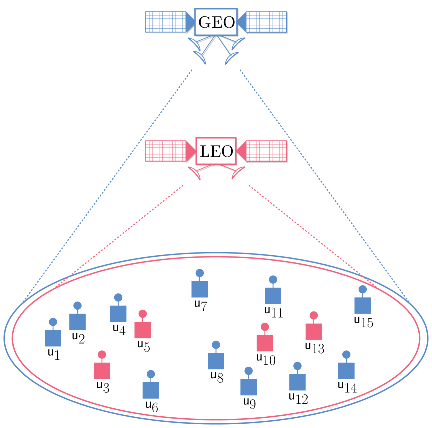
Figure 1: IoT users in simultaneous coverage of a GEO and a LEO satellite.

We consider two scenarios. In scenario ($\mathsf{a}$) each of the two satellite operators utilizes a bandwidth $B$. In this way, the data transmission of each IoT service happens in a different channel, and there is no inter-service multiple-access interference. In scenario ($\mathsf{b}$) instead, the two operators decide to share both channels so that each system coexists over a common bandwidth $2B$.

II-A Random Access Policy

In both scenarios, the chosen multiple access (MAC) policy is CRDSA. Transmissions are slot-synchronous and users, when active, transmit two copies of their physical layer packets within a MAC frame, which is a collection of consecutive time slots. The two packet copies, referred to as replicas, are transmitted by selecting uniformly at random two slots in a MAC frame so that no self-interference is caused. MAC frame examples are given in Fig. 2 case (a). Replicas carry the information about the slot selection enabling the receiver to perform successive interference cancellation (SIC). Each active terminal has $k$ information bits to transmit. The replicas are encoded with a Gaussian codebook. To account for the different propagation distances and receiver characteristics, two coding rates (bits/symbol) are used: $R_{\mathtt{L}}$ for the LEO and $R_{\mathtt{G}}$ for the GEO system. Next, we define $\alpha$ as the ratio:

$$\alpha\triangleq\frac{R_{\mathtt{L}}}{R_{\mathtt{G}}},$$ (1)

with $\alpha\in\mathcal{S}\subset\mathbb{N}$ and $\alpha\geq 1$. Note that packets are transmitted over the same bandwidth $B$ regardless of the scenario and the system considered. Hence, the symbol duration remains fixed and the packet duration for the GEO system will be $\alpha$ times the duration of the replicas in the LEO system. Every replica fits in one LEO or GEO slot and the MAC frame duration is kept the same, thus only some integer values of $\alpha$ are allowed. As illustrated in Fig. 2 case (b), the slot duration may differ between systems. In this way, we denote with ${m}_{\mathtt{L}}$ and ${m}_{\mathtt{G}}$ the number of slots in the MAC frames for the LEO and GEO systems, respectively. The two are related according to ${{{m}_{\mathtt{L}}}/{{m}_{\mathtt{G}}}=\alpha}$. The total number of users accessing the wireless medium is $u=u_{\mathtt{L}}+u_{\mathtt{G}}$, with $u_{\mathtt{L}}$ and $u_{\mathtt{G}}$ being the number of active users served by the LEO and GEO systems, respectively. We define $\beta$ as the ratio between the two. Formally

$$\beta\triangleq\frac{u_{\mathtt{L}}}{u_{\mathtt{G}}}.$$ (2)

The channel load of the system is denoted by $G$ and corresponds to the average number of innovative packets per slot duration. To correctly compute $G$, either the LEO or the GEO slot duration must be taken as reference. Then, the number of active users needs to be appropriately scaled for the other system, e.g. by taking the LEO system perspective:

$$G=\frac{u_{\mathtt{L}}+\alpha u_{\mathtt{G}}}{{m}_{\mathtt{L}}}.$$ (3)

In eq. (3) the GEO traffic spans $\alpha$ LEO slots and thus we account for it as $\alpha u_{\mathtt{G}}$ packets. It can be easily shown that the channel load does not depend on the reference slot duration. The receiver attempts the decoding of the replicas only after the reception of an entire MAC frame. Details on the channel model and decoding condition are discussed in Sec. II-B. A successfully decoded replica provides information about the user slot selections, such that SIC is able to remove both replicas’ contributions from the frame. Ideal interference cancellation is assumed, i.e., no residual interference is left after cancellation. Such a procedure is iterated until no further packets can be decoded. In scenario ($\mathsf{b}$), the two user populations served by LEO and GEO satellites coexist over the same bandwidth. In this setting, it is assumed that the receiver on board each satellite is able to perform SIC on both traffic types.

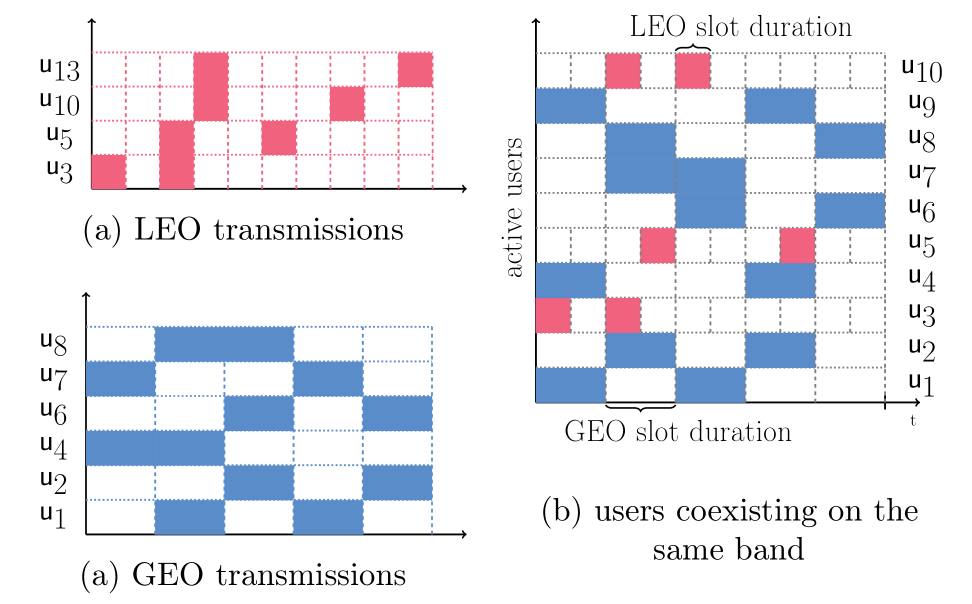
Figure 2: MAC frames where each operator uses a separate channel of bandwidth $B$ are depicted in (a). If operators share the channels, the frames contain mixed traffic on each channel. One such frame is illustrated in (b).

II-B Channel Model and Decoding Condition

We assume an additive white Gaussian noise (AWGN) channel where the attenuation of the transmitted signal is given by free-space path loss, and we consider treat-interference-as-noise (TIN)-SIC decoding within a slot. Hence, we abstract the physical layer by means of an (asymptotic) outage probability model, where a packet is correctly decoded if and only if

$$R_{v}<\bar{\mathsf{I}}_{w},\,\,\text{where }v,w\in\{\mathtt{L},\mathtt{G}\}.$$ (4)

In (4), the average instantaneous mutual information $\bar{\mathsf{I}}$ captures information about the signal-to-noise plus interference ratio experienced by the packet on which we are attempting decoding, hence encapsulating both the interference from other users and the link budget effects. Note that, in (4), $v\in\{\mathtt{L},\mathtt{G}\}$ is used to denote whether a packet is served by the LEO or GEO system. The average instantaneous mutual information must be computed accordingly by setting $w=\mathtt{L}$ when we consider the receiver on-board the LEO satellite and $w=\mathtt{G}$, if decoding is done at the GEO satellite instead. Let us consider a specific replica. We define $P_{w}$ and $N_{w}$ as the received power and noise power, respectively. Moreover, let us denote by $h$ the number of interfering packets over the replica, when decoding a LEO packet, and by $h_{j}$ (with $j=1,2,\ldots,\alpha$) the number of interfering packets over the $j$th length-$m_{\mathtt{L}}$ portion of a packet, when decoding a GEO packet. By assuming perfect power control, i.e., all packets are received with the same power, and with Gaussian codebooks, we have

$$\bar{\mathsf{I}}_{w}= \log_{2}\left(1+\dfrac{P_{w}}{N_{w}+hP_{w}}\right)$$ (5a)

$$\bar{\mathsf{I}}_{w}= \dfrac{1}{\alpha}\displaystyle{\sum_{j=1}^{\alpha}}\log_{2}\left(1+\dfrac{P_{w}}{N_{w}+h_{j}P_{w}}\right)$$ (5b)

where eq. (5a) applies to scenario ($\mathsf{a}$) and for the LEO traffic of scenario ($\mathsf{b}$), while eq. (5b) applies to the GEO traffic of scenario ($\mathsf{b}$). Note that for scenario ($\mathsf{b}$), the GEO traffic coexists with LEO traffic. In this way, packet collisions may affect only a portion of the GEO packet and we shall take this into account in the average mutual information computation. Additionally, for scenario ($\mathsf{a}$) it always holds $v=w$. For scenario ($\mathsf{b}$) instead, the traffic of both systems is received by the LEO and by the GEO. In the following, the signals and noise powers are computed according to the system parameters summarized in Table I. Note that all IoT devices transmit with the same power regardless of the targeted receiver. The lower signal-to-noise ratio (SNR) for the GEO receptions is compensated by setting a lower rate $R_{\mathtt{G}}$. This is similar in effect to using repetitions, as is the case of Narrowband IoT (NB-IoT) [13].

II-C Performance Metric: Maximum Throughput

We are comparing the two scenarios in terms of normalized throughput $S$, i.e. the average number of successfully received information bits per second and per unit of bandwidth. Formally,

$$S_{v}=\begin{cases}\frac{1}{2}R_{v}\,G_{v}\,p_{s,v}(G_{v},R_{v})\quad\text{for scenario~($\mathsf{a}$)}\\ R_{v}\,G_{v}\,p_{s,v}(G_{v},R_{\mathtt{L}},R_{\mathtt{G}},\beta)\quad\text{for scenario~($\mathsf{b}$)}\end{cases}$$ (6)

with $v\in\{\mathtt{L},\mathtt{G}\}$ and where $p_{s}$ is the probability of successful packet reception. In scenario ($\mathsf{a}$), $p_{s}$ is a function of the channel load and the selected rate of the IoT service. In scenario ($\mathsf{b}$) due to the concurrent transmission of the two IoT services over the same band, $p_{s}$ is a function of the load, the rate selected for the LEO and GEO traffic and $\beta$. For scenario ($\mathsf{a}$) we account for the fact that each IoT service gets a bandwidth $B$, effectively being allowed to transmit over only half of the total bandwidth with respect to scenario ($\mathsf{b}$). Finally, the maximum throughput for a selected rate is evaluated according to

$$S^{*}_{v}=\max_{G_{v}}S_{v}.$$ (7)

Thanks to eq. (7) we can investigate how the maximum throughput changes as we vary the selected rates.

III Analytical Approximation of the Maximum Throughput for Scenario ($\mathsf{a}$)

In this section, we develop an analytical approximation of the maximum throughput for scenario ($\mathsf{a}$) by means of density evolution (DE) [14, 15] analysis. The analysis holds in the limit of large frame sizes. Following [15], we introduce a graphical model of the SIC process. In particular, we represent a CRDSA MAC frame with two sets of nodes: user nodes, associated with active users, and slot nodes, associated with slots. An edge connecting a user node $i$ to a slot node $j$ represents the transmission of one packet replica in the $j$th slot by the $i$th user. The node degree represents the number of edges emanating from one node. For the analysis, it is helpful to define the edge-perspective degree distributions $\lambda$ and $\rho$, where $\lambda_{d}$ is the fraction of edges connected to degree-$d$ user nodes, and $\rho_{d}$ is the fraction of edges connected to degree-$d$ slot nodes. In the limit of large frame sizes, we have that slot node degrees are Poisson-distributed, with

$$\rho_{d}=\frac{e^{-2G}(2G)^{d-1}}{(d-1)!}$$ (8)

for $d\geq 1$. Moreover, owing to the two repetitions used by CRDSA, we have that $\lambda_{2}=1$. Now we can leverage DE so to evaluate the SIC performance for asymptotically large frames. We do this by selecting a random user node and developing its neighborhood down to a fixed depth. The resulting graph is tree-like with high probability. We then proceed by evaluating the probability that a user packet is unknown at a given iteration. We refer to the event that decoding of the user packet replica in a slot is unsuccessful as an erasure. We thus track the evolution of the erasure probability over the tree, starting from the leaf nodes, up to the root node (see [15]).

Let us denote by $q_{i}$ the probability that, at the $i$th iteration, an edge carries an erasure message from a user node to a slot node. Furthermore, denote by $p_{i}$ the probability that, at the $i$th iteration, an edge carries an erasure message from a slot node to a user node. We introduce the recursions

$$q_{i} =\mathsf{f}_{\mathsf{u}}(p_{i-1})$$ (9)

$$p_{i} =\mathsf{f}_{\mathsf{s}}(q_{i};G)$$ (10)

which govern the evolution of the erasure probabilities across iterations. Recalling that $\lambda_{2}=1$, we have that [15]

$$\mathsf{f}_{\mathsf{u}}(p_{i-1})=p_{i-1}.$$ (11)

The derivation of (10) requires computing the probability that a user packet replica cannot be decoded over a slot, where $d$ transmissions take place and where each of the transmissions interfering with the packet replica of interest has not been canceled with probability $q_{i}$. We refer to this probability as $\mathsf{f}_{\mathsf{s}}(q_{i};d,G)$. We have that

$$\mathsf{f}_{\mathsf{s}}(q_{i};d,G)=1-\sum_{r=0}^{\tau}\binom{d-1}{r}q_{i}^{r}(1-q_{i})^{d-r-1}$$ (12)

for $d>\tau$, whereas $\mathsf{f}_{\mathsf{s}}(q_{i};d,G)=0$ if $d\leq\tau$, where $\tau$ is the maximum number of colliding packets that can be successfully decoded. Resorting to the intra-slot TIN-SIC model of Section II-B, $\tau$ is simply the largest non-negative integer that satisfies

$$R<\log_{2}\left(1+\dfrac{P}{N+\tau P}\right).$$ (13)

The recursion (10) can be evaluated by averaging (12) over the slot node degree distribution (8). Note that (12) resembles the results in [16].

III-A Computation of $G^{*}$ and Approximation of the Maximum Throughput $\hat{S^{*}}$

The DE analysis proceeds by setting $q_{0}=1$, and by iterating (9) and (10). In particular, due to (11), we can analyze the fixed points of the equation $p_{i}=\mathsf{f}_{\mathsf{s}}(p_{i-1};G)$. We denote by $G^{*}$ the largest value of $G$ for which

$$x>\mathsf{f}_{\mathsf{s}}(x;G)$$ (14)

for all $x\in(0,1)$. This is the largest value of the load for which the erasure probabilities become vanishing small for a large number of iterations. The approximation of the maximum throughput is obtained by

$$\hat{S^{*}}=\frac{R\,G^{*}}{2}$$ (15)

owning to the fact that for scenario ($\mathsf{a}$) only half of the total bandwidth compared to scenario ($\mathsf{b}$) can be utilized. Thanks to the approximation in (15), we are able to evaluate the performance of scenario ($\mathsf{a}$) without the need for extensive numerical simulations. In the next section, we investigate the tightness of the approximation with respect to finite-length numerical results and we show how it is able to accurately predict the rate that maximizes the peak throughput.

IV Results

Monte Carlo simulations have been conducted for both scenarios by setting the parameters described in the model of Section II according to Table I. These values are taken from realistic satellite systems, i.e., Inmarsat F2 satellites for GEO and OneWeb satellites for LEO, whenever available. The SNR at the receiver input results in $5.36$ dB and $-2.99$ dB for the LEO and GEO satellites, respectively.

TABLE I: Simulation Parameters

Description	Symbol	Value	Units
Transmission power	$P_{t}$	23	dBmW
User antenna gain	$\mathsf{G}_{t}$	0	dBi
LEO rx antenna gain	$\mathsf{G}_{r,\mathtt{L}}$	24.2	dBi
GEO rx antenna gain	$\mathsf{G}_{r,\mathtt{G}}$	43.6	dBi
Free space loss for LEO system	$F_{\mathtt{L}}$	161.4	dB
Free space loss for GEO system	$F_{\mathtt{G}}$	190.6	dB
System noise temperature LEO	$T_{s,\mathtt{L}}$	26.4	dBK
System noise temperature GEO	$T_{s,\mathtt{G}}$	25.0	dBK
Bandwidth	$B$	180	kHz
Carrier frequency	$f_{c}$	2	GHz
CRDSA frame size for LEO	${m}_{\mathtt{L}}$	400	slots

Fig. 3 shows the maximum throughput as a function of the rate $R_{\mathtt{L}}$, $R_{\mathtt{G}}$ for each service operating under the assumptions of scenario ($\mathsf{a}$). The CRDSA MAC frame has a duration of ${m}_{\mathtt{L}}={m}_{\mathtt{G}}=400$ slots and each system uses a dedicated channel of bandwidth $B$. Observe that the peak throughput follows a sawtooth profile. This is because we considered a perfect power control scenario and thus the number of colliding packets that can be successfully decoded in the intra-slot SIC varies sharply. As a consequence, any rate smaller than $\log_{2}\left(1+P/(N+hP)\right)$ but larger than $\log_{2}\left(1+P/(N+(h+1)P\right)$ would provide the same performance in terms of successful decoding probability. Hence, the maximum throughput will be directly proportional to the rate for any value within the two aforementioned boundaries. The analytical approximation – red squares and brown diamonds – provides a good estimate of the maximum throughput for finite-length MAC frames along the entire range of rates (within an $8\%$ error). Furthermore, the analytical approximation can predict the rate choice that maximizes the throughput. Note that the choice differs between the LEO and GEO systems due to the dependency on the SNR.

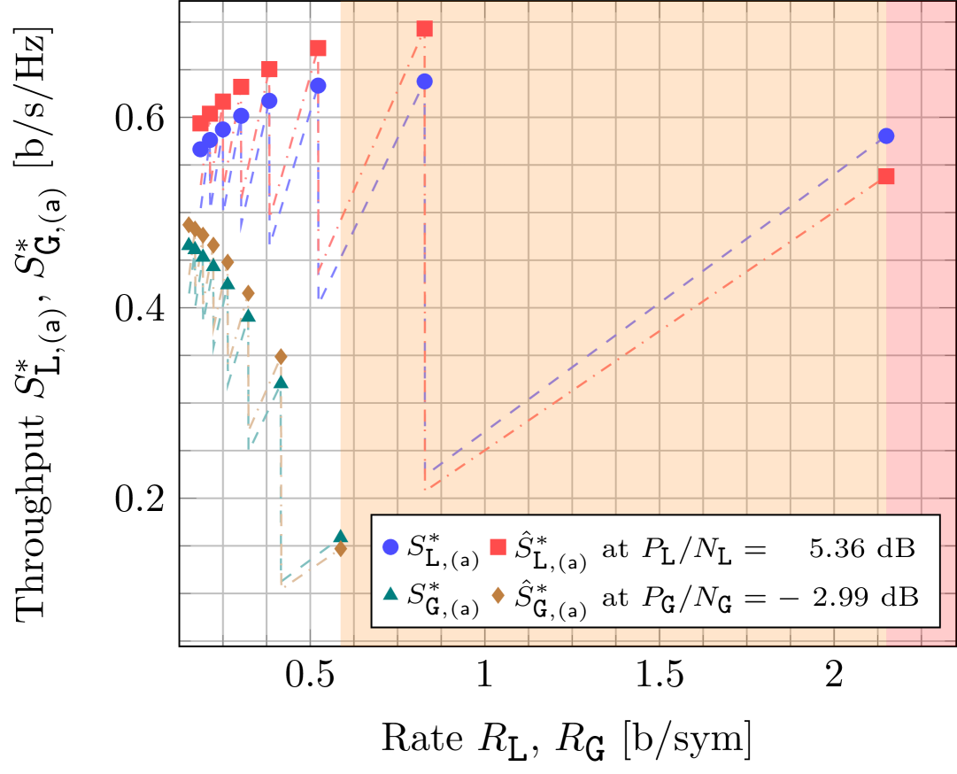
Figure 3: Scenario ($\mathsf{a}$): maximum throughput of LEO traffic received at the LEO satellite and of GEO traffic at the GEO satellite as a function of the rate. Red and orange areas represent the rate values not permitted due to the link budget constraints for the LEO and GEO systems, respectively.

We now investigate the performance of both systems under scenario ($\mathsf{b}$), which assumes that each satellite system accesses the medium with CRDSA on both originally allocated channels at the same time. The discussion is first constrained to the case in which $\beta=1$, where the common satellite coverage area contains the same number of active users serviced by each system. Fig. 4 shows values of maximum throughput grouped according to $\alpha$ for each satellite system when simultaneously sharing the entire band. Each value of throughput is achieved for a specific rate pair $\{R_{\mathtt{L}},R_{\mathtt{G}}\}$. Furthermore, the maximum achievable throughput for each system under scenario ($\mathsf{a}$) is depicted with a dashed line and serves as a benchmark for comparison. The two dashed lines divide the result space into four quadrants of interest. The bottom-left quadrant contains throughput values that are unsatisfactory for both satellite operators, as each would incur a penalty with respect to operating separately on its own band. Consequently, for $\alpha=1$, the operators would be better off by not coexisting. The top-right quadrant, however, depicts the opposite. There are multiple values of $\alpha$ for which the operators have an incentive to coexist, each surpassing the performance it would achieve by operating on segregated bands. We see that the maximum throughput values are achieved for $\alpha=8$. The remaining quadrants represent a conflict of interest. If a throughput pair is in the bottom-right quadrant, the LEO operator would desire coexistence over separation, but exactly the opposite is true for the GEO operator. This holds for a number of rate pairs corresponding to $\alpha\in\{2,4,5\}$. The complementary situation is represented by the top-left quadrant. Here, the GEO operator would rather coexist while the LEO operator would prefer to use its own band exclusively.

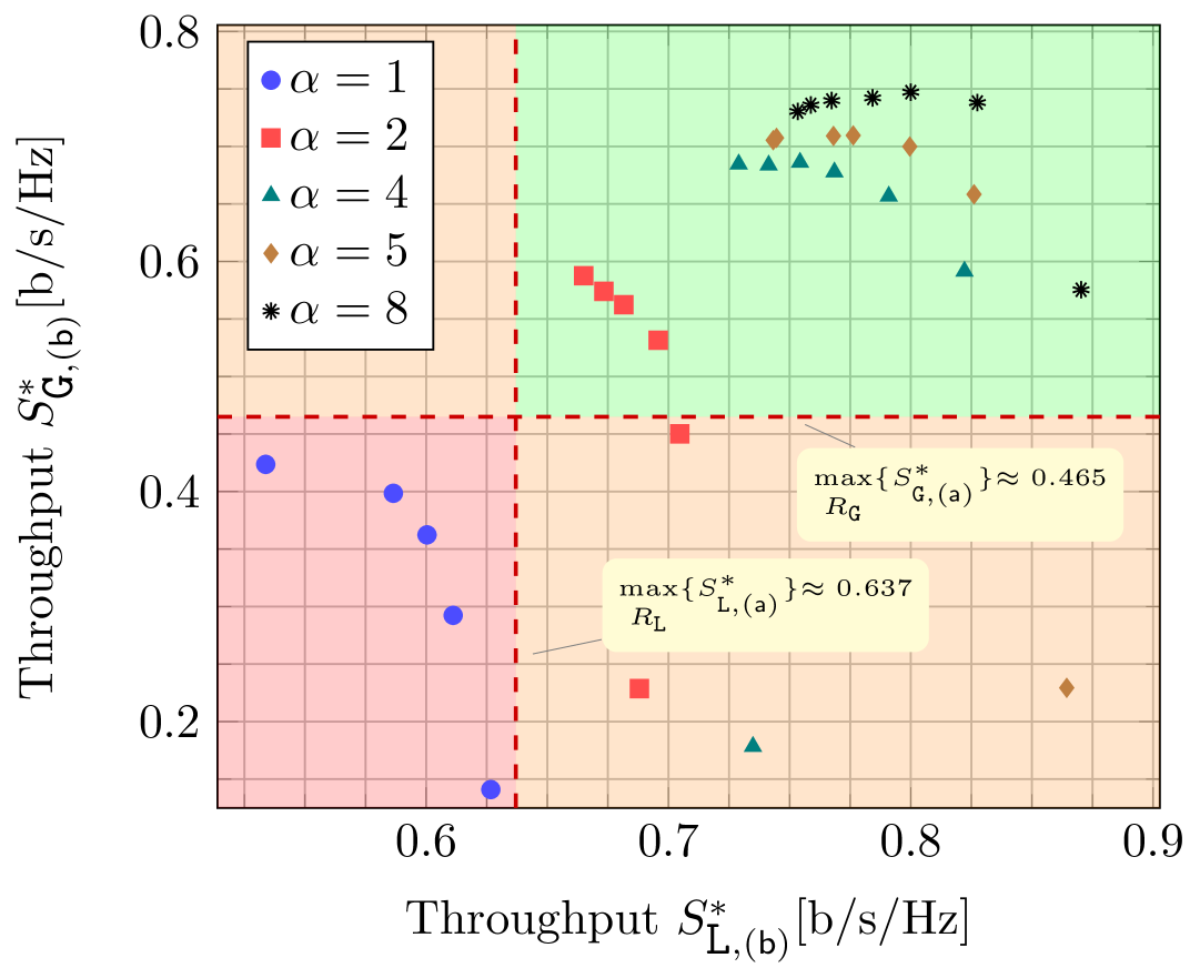
Figure 4: Scenario ($\mathsf{b}$): maximal throughput pairs for $\beta=1$ when both systems coexist on two channels of total bandwidth $B_{s}$.

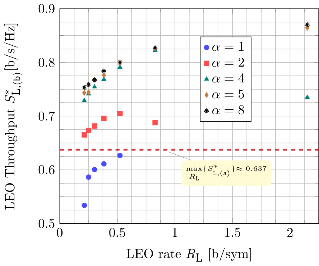
Figure 5: Scenario ($\mathsf{b}$): maximum throughput of LEO traffic received at the LEO satellite for $\beta=1$ as a function of $R_{\mathtt{L}}$ and $\alpha$

In Fig. 5 we inspect the achievable throughput for LEO users for $\beta=1$. For each $\alpha$, there exists a rate choice that maximizes the throughput. Furthermore, despite coexisting with the GEO system, we see that the throughput for the LEO system peaks at $0.870$ [b/s/Hz]. This represents an increase of $36.5\%$ in peak throughput over scenario ($\mathsf{a}$). Similarly, the GEO operator’s performance is captured by Fig. 6, which shows that the throughput values are trending roughly inversely proportional to the rate values available for the GEO users. A peak throughput of $0.747$ [b/s/Hz] is also achieved for $\alpha=8$, which marks a gain of $60.6\%$ over the peak throughput value of scenario ($\mathsf{a}$). While each operator can agree to choose a rate that results in $\alpha=8$, it does not achieve maximum throughput for the same rate pair as the competitor. A mechanism needs to be devised to let the operators agree on a suitable rate pair.

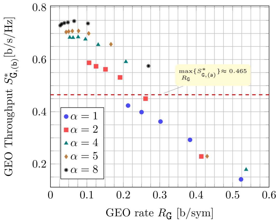
Figure 6: Scenario ($\mathsf{b}$): Maximum throughput of GEO traffic received at the GEO satellite for $\beta=1$ as a function of $R_{\mathtt{G}}$ and $\alpha$.

We now expand the discussion to include results for a case where more active users are serviced by the LEO operator than the GEO one, i.e., for $\beta=4$; and results for the mirrored case, namely for $\beta=0.25$. Fig. 7 shows three sets of throughput pairs corresponding to different $\beta$. Red circular markers correspond to $\beta=0.25$, black diamond markers to $\beta=1$, and blue triangular markers to $\beta=4$. This figure is also divided into four quadrants with the same meaning as per Fig. 4. Should the number of users served by the GEO operator be four times the number serviced by the LEO operator ($\beta=0.25$), then there are no throughput pairs available that would incentivize the LEO operator to choose coexistence, as all throughput values are lower than the peak throughput of scenario ($\mathsf{a}$). The GEO operator, on the other hand, has points available that express a desire for coexistence (top left quadrant). Finally, should $\beta=4$, a case where there are four times as many LEO users than GEO users, then the LEO operator would always prefer to coexist with the GEO (top-right and bottom-right quadrants). The mutual desire to coexist, however, is given when $\alpha=8$. This latter case is represented by throughput pairs marked with blue triangles, which are exclusively located in the top-right quadrant.

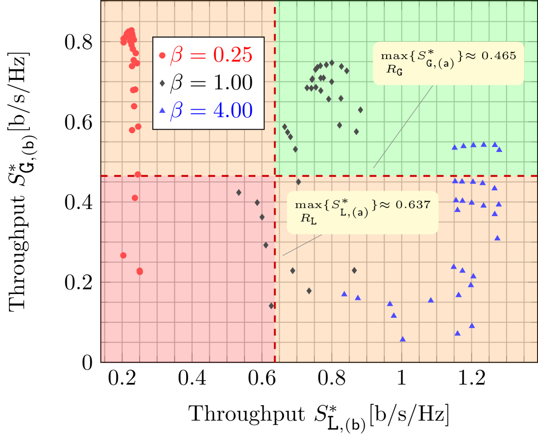
Figure 7: Scenario ($\mathsf{b}$): maximum throughput pairs for $\beta=1/4,~\beta=1$ and $\beta=4$ when both systems coexist on two channels of joint bandwidth $B_{s}$.

V Conclusions

This paper has studied the problem of whether it is better for two distinct satellite operators – one employing exclusively LEO satellites, while the other, just GEO satellites – to share their originally allocated frequency bands and have their users coexist or to keep their allocated band exclusively for themselves. The use-case under consideration is servicing IoT devices in a remote monitoring scenario with bursty traffic which deploys a modern random access policy i.e., CRDSA. We have found that for carefully selected channel code rates, each individual IoT service has a sizeable benefit in the peak throughput by sharing its band. We observed a gain of up to 36.5% for the LEO operator and of up to 60.6% for the GEO operator in peak throughput with respect to the case where each keeps its traffic on the original allocated band.

References

- [1] F. Rinaldi, H.-L. Maattanen, J. Torsner, S. Pizzi, S. Andreev, A. Iera, Y. Koucheryavy, and G. Araniti, “Non-Terrestrial Networks in 5G & Beyond: A Survey,” IEEE Access, vol. 8, pp. 165 178–165 200, 2020.
- [2] A. Guidotti, A. Vanelli-Coralli, M. El Jaafari, N. Chuberre, J. Puttonen, V. Schena, G. Rinelli, and S. Cioni, “Role and Evolution of Non-Terrestrial Networks Toward 6G Systems,” IEEE Access, 2024.
- [3] E. Commision, “Iris2: the new EU secure satellite constellation,” 2024, https://defence-industry-space.ec.europa.eu/eu-space/iris2-secure-connectivity_en [Accessed: 30.04.2025].
- [4] M. Centenaro, C. E. Costa, F. Granelli, C. Sacchi, and L. Vangelista, “A Survey on Technologies, Standards and Open Challenges in Satellite IoT,” IEEE Commun. Surveys Tuts., vol. 23, no. 3, pp. 1693–1720, 2021.
- [5] “Ericsson mobility report data and forecasts, IoT connections outlook,” Ericsson, https://www.ericsson.com/en/reports-and-papers/mobility-report/dataforecasts/iot-connections-outlook, techreport, Nov. 2022.
- [6] L. Zhang, Y.-C. Liang, and M. Xiao, “Spectrum Sharing for Internet of Things: A Survey,” IEEE Wireless Commun., vol. 26, no. 3, pp. 132–139, 2019.
- [7] H. Pirayesh, P. K. Sangdeh, and H. Zeng, “Coexistence of Wi-Fi and IoT Communications in WLANs,” IEEE Internet Things J., vol. 7, no. 8, pp. 7495–7505, 2020.
- [8] F. Clazzer, H. Fuchs, and M. Grec, “Coexistence of IoT Networks in 6G: A MAC Study for 3D NTN Architectures,” in Proc. IEEE Intl. Conf. on Comm. (ICC) WS, 2024, pp. 1462–1468.
- [9] P. Popovski, K. F. Trillingsgaard, O. Simeone, and G. Durisi, “5G Wireless Network Slicing for eMBB, URLLC, and mMTC: A Communication-Theoretic View,” IEEE Access, vol. 6, pp. 55 765–55 779, 2018.
- [10] B. Qian, H. Zhou, T. Ma, K. Yu, Q. Yu, and X. Shen, “Multi-Operator Spectrum Sharing for Massive IoT Coexisting in 5G/B5G Wireless Networks,” IEEE J. Sel. Areas Commun., vol. 39, no. 3, pp. 881–895, 2021.
- [11] A. Munari and F. Clazzer, “Spectral Coexistence of QoS-Constrained and IoT Traffic in Satellite Systems,” Sensors, vol. 21, no. 14, 2021.
- [12] E. Casini, R. De Gaudenzi, and O. del Rio Herrero, “Contention Resolution Diversity Slotted ALOHA (CRDSA): An Enhanced Random Access Scheme for Satellite Access Packet Networks,” IEEE Trans. Wireless Commun., vol. 6, no. 4, pp. 1408–1419, Apr. 2007.
- [13] M. Kanj, V. Savaux, and M. Le Guen, “A Tutorial on NB-IoT Physical Layer Design,” IEEE Commun. Surveys Tuts., vol. 22, no. 4, pp. 2408–2446, 2020.
- [14] T. J. Richardson, M. A. Shokrollahi, and R. L. Urbanke, “Design of capacity-approaching irregular low-density parity-check codes,” IEEE Trans. Inf. Theory, vol. 47, no. 2, pp. 619–637, Feb. 2001.
- [15] G. Liva, “Graph-Based Analysis and Optimization of Contention Resolution Diversity Slotted ALOHA,” IEEE Trans. Commun., vol. 59, no. 2, pp. 477–487, Feb. 2011.
- [16] F. Clazzer, E. Paolini, I. Mambelli, and Č. Stefanović, “Irregular Repetition Slotted ALOHA over the Rayleigh Block Fading Channel with Capture,” in Proc. IEEE Intl. Conf. on Comm. (ICC), Paris, France, May 2017, pp. 1–6.