Automated Test Oracles for Flaky Cyber-Physical System Simulators: Approach and Evaluation

Abstract

Simulation-based testing of cyber-physical systems (CPS) is costly due to the time-consuming execution of CPS simulators. In addition, CPS simulators may be flaky, leading to inconsistent test outcomes and requiring repeated test re-execution for reliable test verdicts. Automated test oracles that do not require system execution are therefore crucial for reducing testing costs. Ideally, such test oracles should be interpretable to facilitate human understanding of test verdicts, and they must be robust against the potential flakiness of CPS simulators. In this article, we propose assertion-based test oracles for CPS as sets of logical and arithmetic predicates defined over the inputs of the system under test. Given a test input, our assertion-based test oracle determines, without requiring test execution, whether the test passes, fails, or if the oracle is inconclusive in predicting a verdict. We describe two methods for generating assertion-based test oracles: one using genetic programming (GP) that employs well-known spectrum-based fault localization (SBFL) ranking formulas, namely Ochiai, Tarantula, and Naish, as fitness functions; and the other using decision trees (DT) and decision rules (DR). We evaluate our assertion-based test oracles through case studies in the domains of aerospace, networking and autonomous driving. We show that test oracles generated using GP with Ochiai are significantly more accurate than those obtained using GP with Tarantula and Naish or using DT or DR. Moreover, this accuracy advantage remains even when accounting for the flakiness of the system under test. We further show that the assertion-based test oracles generated by GP with Ochiai are robust against flakiness with only 4% average variation in their accuracy results across four different network and autonomous driving systems with flaky behaviours.

I Introduction

Testing cyber-physical systems (CPS) typically relies on simulators, which may be virtual or hybrid combinations of hardware and software [1]. Executing tests with these simulators is often expensive and time-consuming. Moreover, simulators are inherently non-deterministic due to environmental variability, unpredictable hardware–software interactions, and stochastic processes. As a result, the same inputs may yield different outputs across executions, causing flakiness in test outcomes [2, 3, 4, 5, 6]. Flakiness – where a test non-deterministically passes or fails – has been observed in domains such as autonomous vehicles, drones, and networked systems. Due to flakiness, engineers may need to run a test multiple times to determine whether it passes or fails. The need to re-run tests, coupled with the high cost of executing CPS simulators, results in substantial overall costs for using test oracles that rely on test executions to determine pass or fail verdicts.

Several approaches automate test oracles through data-driven methods, using supervised machine learning (ML) models trained on data from test executions labelled as pass or fail verdicts. For example, automated test oracles have previously been generated using neural networks [7, 8, 9, 10, 11, 12] and adaptive boosting [13, 14], as well as decision trees, support vector machine and Naïve Bayes [14]. We identify three key limitations in these existing approaches: First, with the exception of a few strands of relatively recent work [12, 7], earlier studies have focused on reducing the cost of human oracles rather than decreasing the number of system executions, and still require executions to determine all test verdicts. This makes such techniques of limited applicability in settings – such as CPS simulators – where system executions are expensive and resource-intensive. Second, apart from decision trees, the ML models previously used as test oracles are not interpretable. In particular, the approaches described in [12, 7] rely on neural networks, which are inherently non-interpretable. Since most CPS undergo stringent quality assurance processes, such as safety certification, it is crucial that the ML models used for test oracle automation be interpretable. This interpretability allows humans to understand how specific test verdicts are determined based on the models’ internal mechanisms. Third, due to the flakiness of CPS simulators, some test verdicts in the training sets used for learning test oracles may be unreliable; that is, the same test input may produce different verdicts upon re-execution. Consequently, test oracles trained on datasets containing identical inputs but inconsistent verdicts may produce less stable and reliable predictions, showing reduced robustness – that is, a reduced ability to provide consistent verdicts for the same inputs. To our knowledge, no prior study has evaluated how flakiness in test verdicts impacts the robustness of test oracles obtained through data-driven techniques.

In this article, we propose assertion-based test oracles for CPS, defined as sets of logical and arithmetic predicates over the inputs of the system under test (SUT). Given a test input, an assertion-based test oracle determines – without requiring system execution – whether the test passes, fails, or if the oracle is inconclusive in predicting a verdict. When the oracle is inconclusive, system execution becomes necessary.

Figure 1(a) shows the classical workflow for verdict assignment: the SUT is executed on a test input to produce an output. A test oracle, typically developed based on system requirements, assesses the input and output to determine the verdict. This workflow requires executing the SUT for each test input, which, as we argued earlier, can be costly for CPS. In contrast, Figure 1(b) shows the workflow for verdict assignment with assertion-based test oracles. These oracles directly evaluate test inputs and determine a pass or fail verdict when possible without executing the SUT. If the oracle is inconclusive, the SUT must, of course, be executed.

As we will see in detail in Section II, assertion-based test oracles are sets of individual assertions constructed so that the set never issues conflicting verdicts. An example of an assertion used in an assertion-based test oracle for an autonomous driving system (ADS) with inputs such as ego-vehicle speed and road angle is: $\mathit{road\_angle}>64^{\circ}\land\mathit{speed}\geq 100\ \mathit{km/h}\Rightarrow\mathit{fail}$. This assertion states that any test input in which the ego vehicle is travelling at least 100 km/h on a sharply turning road (angle greater than $64^{\circ}$), will result in the vehicle veering out of its lane, leading to a failure. In this assertion, the expression $\mathit{road\_angle}>64^{\circ}\land\mathit{speed}\geq 100\ \mathit{km/h}$ represents the condition, while $\mathit{fail}$ denotes the verdict. The verdict for any test input satisfying the condition is fail.

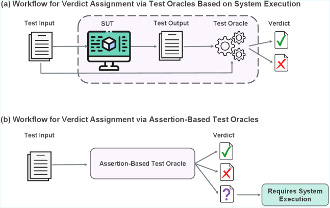
Figure 1: Workflow for verdict assignment using (a) test oracles based on system execution, (b) assertion-based test oracles which avoid system execution when possible. Symbols indicate: ✓ for a pass verdict, ✗ for a fail verdict and ? for an inconclusive verdict. For inconclusive verdicts, system execution is required to determine a pass or fail verdict.

We propose two methods for generating assertions such as the one illustrated above: one based on genetic programming (GP) and the other using interpretable machine learning techniques, specifically decision trees (DT) and decision rules (DR). We use these methods to learn assertions from training sets of test inputs labelled with pass or fail verdicts such that the learned assertions explain these verdicts in the training data. DT and DR are known for their ability to derive classification conditions from data. DT creates a hierarchical, tree-like structure of decisions, while DR establishes a set of if-then rules for classification based on input variables. GP, on the other hand, is an evolutionary algorithm that iteratively evolves complex structures using a fitness function to optimize them for a particular objective. In our work, we employ GP to evolve candidate conditions, such as $\mathit{road\_angle}>64^{\circ}\land\mathit{speed}\geq 100\ \mathit{km/h}$, to identify those that best explain the pass and fail verdicts within the training data.

Contributions. Our contributions are as follows:

(i) We introduce assertion-based test oracles for CPS as sets of assertions that determine pass or fail verdicts whenever it is possible to do so without executing the CPS (Section II-A). Our assertion-based test oracles ensure three important properties: (1) consistency of predicted verdicts, (2) effectiveness in distinguishing passing from failing behaviours, and (3) applicability to signal-based CPS:

1. Combining assertions into a set requires ensuring that the collection remains consistent in the verdicts it issues. Assertions from DT are consistent by construction, whereas those from DR and GP may conflict, since these techniques independently generate assertions for passing and failing behaviours. We propose a pruning mechanism that enforces consistency by preventing assertion-based test oracles from assigning conflicting verdicts (Section III-C).

2. To improve the effectiveness of the test oracles generated using GP, we use spectrum-based fault-localization (SBFL) ranking formulas as the fitness functions of GP (Section III-A2). Specifically, we adopt three well-known SBFL ranking formulas from the literature [15, 16, 17, 18], namely Ochiai, Tarantula, and Naish. These formulas rank the suspiciousness of program statements based on their involvement in passing and failing executions. This ranking mechanism aligns with our goal of deriving assertions from training data that differentiate passing from failing behaviours.

3. To show the applicability of our assertion-based test oracles to signal-based CPS, we present a formal characterization of the expressive power of these oracles in capturing common CPS signal properties (Section IV). We formally show that, for CPS with piecewise-constant input signals, our assertions capture all logical operators as well as the “globally” temporal operator from Signal Temporal Logic (STL) [19]. In addition, our assertions can express arithmetic operations within predicates, which are not part of the core STL formula syntax, thereby extending STL with explicit support for arithmetic expressions. This level of expressiveness is sufficient to capture 85 of the 98 requirements in the Lockheed Martin benchmark [20], as formalized by Menghi et al. [21]. The assumption of piecewise-constant input signals is widely adopted in CPS benchmarks and case studies in the literature [20, 22, 23, 24, 25, 26].

(ii) We empirically evaluate assertion-based test oracles across five different network, autonomous-driving and aerospace systems (Section V), assessing the accuracy and robustness of the test oracles. Accuracy measures how well test oracles predict actual verdicts for unseen test inputs. Inaccuracies occur when actual fail verdicts are wrongly predicted as pass, and actual pass verdicts are wrongly predicted as fail. Robustness is the extent to which test oracles, trained on datasets with identical inputs but inconsistent verdicts due to flakiness, produce consistent predictions. We measure robustness as the variation in prediction accuracy across multiple test oracles trained on datasets with identical test inputs but inconsistent pass or fail verdicts due to flakiness. Our robustness analysis aims to determine whether flaky tests – due to potentially unreliable verdicts – should be excluded from the initial training set used to develop test oracles, or whether they can remain because their inclusion has minimal impact on the accuracy of the resulting test oracle. Our main findings are:

1. Using GP with Ochiai is most effective for generating assertion-based test oracles. Specifically, test oracles generated by GP with Ochiai are significantly more accurate than those generated by GP with Tarantula or Naish, as well as those generated by DT and DR. Furthermore, GP with Ochiai misclassifies fewer failing tests as passing compared to other techniques, thus reducing the likelihood of masking failures as passes (RQ2 in Section V).

2. When using GP with Ochiai, the average variation in test oracle accuracy is approximately 4%. This indicates that the impact on the prediction accuracy of test oracles, caused by pass or fail label inconsistencies, is on average 4%. If such variation is acceptable, practitioners can forgo removing flaky tests – which require multiple test executions – from the initial training set, thus reducing costs (RQ3 in Section V).

Our full replication package is available online [27].

Organization. Section II defines assertion-based test oracles, presents their construction and provides an overview of their evaluation. Section III describes our data-driven framework for deriving assertion-based test oracles, presents alternative approaches using GP and ML to generate assertion-based test oracles, and introduces our pruning strategy for obtaining a consistent set of assertions as a test oracle. Section IV presents assertion-based test oracles for signal-based CPS, focusing on specifying assertions over signals and their expressiveness, with a running example. Section V presents an evaluation of the alternative approaches (GP and ML) for generating assertion-based test oracles. Section VI outlines how our approach can be used in practice. Section VII compares with related work. Section VIII concludes the article.

II Assertion-based Test Oracles

We define and illustrate assertion-based test oracles in Section II-A, and then provide an overview of their construction and evaluation in Sections II-B and II-C, respectively.

II-A Definition

A test oracle is a mechanism that determines a pass or fail verdict for a given test input to a system $S$. Given a system requirement, a test input fails if executing the system with that input produces behaviour that violates the requirement; otherwise, the test input passes. As noted in Section I, our goal is to develop interpretable test oracles that infer verdicts from test inputs. To this end, we propose assertion-based test oracles, formally defined and exemplified in this section.

Definition 1 (Assertion).

An assertion for a system $S$, is an expression of the form $\mathit{condition}\Rightarrow\mathit{verdict}$, where $\mathit{condition}$ is a logical predicate over the inputs of $S$ and $\mathit{verdict}$ is either pass or fail.

For a test input $t$, the assertion $\mathit{condition}\Rightarrow\mathit{fail}$ implies that if $t$ satisfies $\mathit{condition}$, then the verdict for $t$ is fail. Similarly, the assertion $\mathit{condition}\Rightarrow\mathit{pass}$ implies that if $t$ satisfies $\mathit{condition}$, then the verdict for $t$ is pass. We refer to an assertion with a fail verdict as a fail assertion and an assertion with a pass verdict as a pass assertion.

For example, Figure 2 illustrates two pass assertions ($a_{1}$ and $a_{3}$) and one fail assertion ($a_{2}$) for a simplified autonomous driving system (ADS). ADS has one requirement stating that the ego vehicle must not collide with non-ego vehicles. The simplified ADS has four inputs: ego-vehicle speed (denoted by $\mathit{speed}$), the degree of road’s steepness ($\mathit{road\_slope}$), the hour of the day ($\mathit{time\_of\_day}$), and the number of nearby non-ego vehicles ($\mathit{other\_vehicles}$).
As shown in Figure 2, six test inputs $t_{1}$ to $t_{6}$ are provided for the ADS, each assigning specific values to its four inputs. The three assertions ($a_{1}$, $a_{2}$ and $a_{3}$) in Figure 2 constitute an assertion-based test oracle and can determine pass or fail verdicts based on test inputs only, thus avoiding ADS execution whenever possible. For example, test input $t_{1}$ passes since the input values in $t_{1}$ satisfy the condition of assertion $a_{1}$, i.e., $\mathit{speed}\leq 20\land\mathit{road\_slope}<2\land\mathit{other\_vehicles}=0$. The condition for $a_{1}$ is a logical predicate over inputs $\mathit{speed}$ and $\mathit{road\_slope}$ and $\mathit{other\_vehicles}$, stating that tests where the ego vehicle is moving uphill at a speed of at most $20$ km/h, on a road with a slope of less than $2$ degrees and with no nearby non-ego vehicles, do not lead to any collision. Hence these tests satisfy the ADS requirement and are passing.

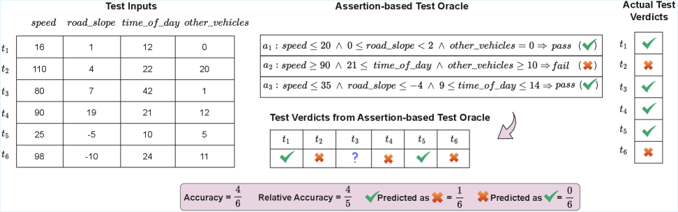
Figure 2: An assertion-based test oracle for a simplified ADS with inputs $\mathit{speed}$, $\mathit{road\_slope}$, $\mathit{time\_of\_day}$ and $\mathit{other\_vehicles}$, along with an example set of test inputs for this system. In this figure, ✓ indicates the pass verdict, ✗ indicates the fail verdict and ? indicates that the verdict is inconclusive.

Definition 2 (Assertion-based Test Oracle).

An assertion-based test oracle $\mathcal{O}$ for a system $S$ is a set of assertions defined for $S$ whose members are pairwise consistent. Two assertions $\mathit{cnd}\Rightarrow\mathit{v}$ and $\mathit{cnd}^{\prime}\Rightarrow\mathit{v^{\prime}}$ are consistent if $v\neq v^{\prime}$ implies that the conjunction $\mathit{cnd}\wedge\mathit{cnd}^{\prime}$ is unsatisfiable (UNSAT).

Definition 2 ensures that a test oracle based on a set of assertions is consistent in the verdicts it predicts. While a test input $t$ may satisfy the conditions of multiple assertions, all such assertions must agree on the verdict – either all pass or all fail. For example, in Figure 2, assertions $a_{1}$, $a_{2}$ and $a_{3}$ form a consistent assertion-based test oracle because their condition conjunctions (i.e., $a_{1}\wedge a_{2}$ and $a_{2}\wedge a_{3}$) are unsatisfiable. However, if we add a fail assertion $a_{4}:\mathit{speed}>15\ \land\ \mathit{road\_slope}\geq 1\Rightarrow\mathit{fail}$, the oracle becomes inconsistent because the conjunction of conditions of $a_{1}$ and $a_{4}$ is satisfiable and these assertions predict opposing verdicts (pass and fail, respectively).

The verdict assigned by an assertion-based test oracle $\mathcal{O}$ for a test input $t$ is determined as follows:

$$\begin{cases}\mathit{fail}&\text{if }\exists(\mathit{cnd}\Rightarrow\mathit{fail})\in\mathcal{O}\ s.t.\ t\models\mathit{cnd}\\ \mathit{pass}&\text{if }\exists(\mathit{cnd}\Rightarrow\mathit{pass})\in\mathcal{O}\ s.t.\ t\models\mathit{cnd}\\ \mathit{inconclusive}&\text{otherwise}\end{cases}$$

Specifically, if $t$ satisfies the condition of any pass assertion ($\mathit{cnd}\Rightarrow\mathit{pass}$) in $\mathcal{O}$, then the verdict for $t$ is pass. Dually, if $t$ satisfies the condition of any fail assertion ($\mathit{cnd}\Rightarrow\mathit{fail}$) in $\mathcal{O}$, then the verdict for $t$ is fail. Since the test oracle $\mathcal{O}$ is consistent, when $t$ satisfies multiple assertions, all such assertions agree on the same verdict. If $t$ does not satisfy the condition of any assertion in $\mathcal{O}$, the verdict is considered inconclusive. For example, among the six test inputs ($t_{1}$ to $t_{6}$) shown in Figure 2, the assertion-based test oracle, composed of assertions $a_{1}$ to $a_{3}$, implies that $t_{1}$ and $t_{5}$ pass as they satisfy the conditions for $a_{1}$ and $a_{3}$, respectively. Test inputs $t_{2}$, $t_{4}$ and $t_{6}$ fail as they satisfy the condition of $a_{2}$. The test oracle is inconclusive for $t_{3}$ as this test input does not satisfy the conditions of any assertions in the test oracle.

II-B Test-Oracle Construction and Verdict Thresholds

To construct assertion-based test oracles, we adopt a data-driven approach that infers assertions from training data consisting of test inputs and their corresponding pass/fail verdicts. Because these assertions are learned from finite datasets, each is associated with a confidence level – expressed as a probability – that reflects the assertion’s reliability in predicting a verdict based on the training data. Specifically, the confidence level of an assertion is defined as its precision in classifying pass or fail tests in the training data. Given an assertion and its associated confidence, we must decide whether the confidence level is sufficient for the assertion to be included in a test oracle for verdict prediction. To this end, we introduce a user-defined lower bound, called the verdict threshold:

Definition 3 (Verdict threshold).

Let $\mathcal{O}$ be an assertion-based test oracle constructed using a data-driven approach. The verdict threshold $\theta$ is a minimum confidence level such that only assertions whose confidence levels meet or exceed $\theta$ are retained in $\mathcal{O}$ for predicting test verdicts.

For example, Figure 3 shows two test oracles, each consisting of the assertions $a_{1}$, $a_{2}$, and $a_{3}$ with confidence levels of 70%, 85%, and 90%, respectively. Assuming that the verdict threshold $\theta$ is set to 70% for the test oracle in Figure 3(a), all assertions $a_{1}$ through $a_{3}$ are included. However, in Figure 3(b), when the verdict threshold $\theta$ is raised to 80%, only assertions $a_{2}$ and $a_{3}$ are included.

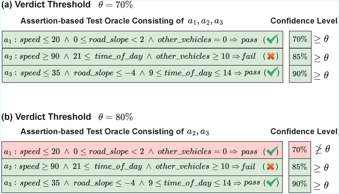
Figure 3: Confidence levels for assertions $a_{1}$, $a_{2}$ and $a_{3}$ in Figure 2, where (a) at a verdict threshold of $\theta=70\%$, all assertions are included in the test oracle, and (b) at a verdict threshold of $\theta=80\%$, only assertions $a_{2}$ and $a_{3}$ are included in the test oracle.

II-C Overview of Assertion-based Test Oracle Evaluation

As discussed in Section I, we evaluate assertion-based test oracles in terms of their accuracy and robustness. This assessment is performed against a ground-truth test oracle, which, as defined by Barr et al. [28], is a “total oracle that always gives the right answer”. A total oracle provides conclusive pass or fail verdicts for all test inputs. Accuracy and robustness are measured by comparing the verdicts predicted by the test oracles against those of the ground-truth oracle. In our work, the ground-truth verdicts are obtained by executing the actual SUT for each test input.

To evaluate the accuracy of test oracles, we measure prediction correctness in two ways: (1) over all predictions, including inconclusive ones, and (2) only over conclusive predictions. For these two cases, we define two metrics: accuracy, the percentage of correctly predicted verdicts across all tests, and relative accuracy, the percentage restricted to conclusive predictions. Accuracy reflects losses from both inconclusive and incorrect predictions, while relative accuracy isolates losses due only to incorrect predictions. We also define the misprediction rate as the percentage of incorrectly predicted verdicts across all tests, distinguishing between (1) passing tests wrongly predicted as failing and (2) failing tests wrongly predicted as passing.
For example, based on the actual (ground-truth) test verdicts shown on the right of Figure 2, the predicted verdicts for $t_{1}$, $t_{2}$, $t_{5}$, and $t_{6}$ are correct, the verdict for $t_{4}$ is incorrect, and the verdict for $t_{3}$ cannot be predicted conclusively. Thus, the accuracy of the test oracle in Figure 2 is $\frac{4}{6}$ and its relative accuracy is $\frac{4}{5}$. In addition, the rate of the pass tests wrongly predicted as fail and the rate of fail tests wrongly predicted as pass of the test oracle in Figure 2 are $\frac{1}{6}$ and $\frac{0}{6}$, respectively.
To evaluate the robustness of test oracles, we measure the variation in prediction accuracy across multiple test oracles trained on datasets with identical test inputs but inconsistent pass/fail verdicts due to flakiness. A robust test oracle should maintain consistent accuracy, showing minimal variation despite such inconsistencies in the training data. In Section V, we evaluate different techniques for generating assertion-based test oracles using the metrics introduced in this section, with RQ2 focusing on accuracy and RQ3 focusing on robustness.

III Generating Assertion-based Test Oracles

Figure 4 shows an overview of GenTC, our framework for deriving assertion-based test oracles. The framework has three steps. The first step of GenTC uses adaptive random testing [29] to generate a training set of test inputs. Adaptive random testing randomly samples test inputs from the search space by maximizing the Euclidean distance between the sampled test inputs, hence increasing diversity among the generated tests [29]. To label these test inputs as either pass or fail, they are executed on the SUT.

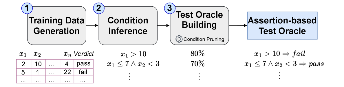
Figure 4: Our approach for deriving assertion-based test oracles

The second step of GenTC uses the training data generated in the first step to learn conditions for assertions. Recall from Definition 1 that conditions are logical predicates defined over SUT’s inputs. For example, $\mathit{speed}\leq 20\ \land\ 0\leq\mathit{road\_slope}<2\ \land\ \mathit{other\_vehicles}=0$ is a condition for assertion $a_{1}$ in Figure 2. This step identifies conditions that best explain pass elements or fail elements in the training data. We consider two alternatives for condition inference: (1) using genetic programming (GP) presented in Sections III-A, and (2) using Decision Trees (DT) and Decision Rules (DR) presented in Section III-B. The third and final step of GenTC, described in Section III-C, introduces a pruning mechanism to ensure the consistency of assertion-based test oracles.

III-A Condition Inference by Genetic Programming (GP)

The first alternative we consider to generate conditions defined over the SUT’s input variables is GP. GP requires a grammar to define its candidate solutions, which in our work, are conditions based on the SUT’s input variables. Below, we first present the grammar that GenTC uses for GP, followed by an explanation of how GP learns conditions that conform to this grammar.

III-A1 Grammar Specification

We provide a grammar that captures conditions over the input variables of the SUT. Given that our work focuses on CPS, where inputs are typically numeric [30, 31], we adopt the following grammar (denoted by $\mathcal{G}$), which has previously been used to define environmental assumptions for CPS [31] and to specify control logic for network systems [32]:

or-term	:: =	or-term $\vee$ or-term $|$ and-term
and-term	:: =	and-term $\wedge$ and-term $|$ rel-term
rel-term	:: =	exp $<$ $0$ $|$ exp $\leq$ $0$ $|$ exp $>$ $0$ $|$ exp $\geq$ $0$ $|$ exp $=$ $0$ $|$ exp $\neq$ $0$
exp	:: =	exp $+$ exp $|$ exp $-$ exp $|$ exp $*$ exp $|$ exp $/$ exp $|$ const $|$ cp

Figure 5: Syntactic rules of the grammar (denoted by $\mathcal{G}$) that define the assertions over system input variables.

The symbol $|$ in the above grammar separates alternatives, const is an ephemeral random constant generator [33] and cp represents an input variable of the SUT. This grammar generates conditions that are either conjunctions of relational expressions over arithmetic terms or disjunctions of such conjunctions.

III-A2 Condition Learning

Algorithm 1 describes our GP-based condition inference algorithm. The inputs to Algorithm 1 are a training set $TS$ generated by the first step of GenTC (Figure 4) and a fitness function $F$ that guides GP to generate conditions that best explain pass or fail results in the training set. Depending on the fitness function $F$, Algorithm 1 either generates conditions that explain the fail results or conditions that explain the pass results. In order to have assertions for both pass and fail verdicts such as those in Figure 2, as we discuss below, we need to execute Algorithm 1 with dual fitness functions designed to generate pass and fail conditions separately.

Algorithm 1 begins by creating an initial population $P_{0}$ (line $2$) of possible conditions (individuals). Each individual is then evaluated using the input fitness function (line $3$). The population is evolved by breeding a new offspring population (line $5$), which is added to the current population. The algorithm uses tournament selection to choose individuals from the population (line $7$) for the next generation’s breeding and evaluation. These steps are repeated until a specified number of generations is reached. Finally, the algorithm returns the individuals with the best fitness values (lines $10$–$11$).

Algorithm 1 Condition Inference by GP

Input $\mathit{TS}$: Training Set
Input $F$: Fitness function for GP
Output $C$: Set of conditions explaining the test outcomes

1: $t\leftarrow$ 0;

2: $\mathit{P_{0}}\leftarrow$ Initialize(); //Initialize the GP population

3: $\mathit{P_{0}.Fit}\leftarrow$ Evaluate($\mathit{P_{0}}$, $\mathit{TS}$, $F$); //Calculate the fitness values of GP individuals. $F$ is a function from Figure 6.

4: while $\neg(\textit{stop condition})$ do

5:  $\mathit{off}\leftarrow$ Breed($P_{t}$);

6:  $\mathit{off.Fit}\leftarrow$ Evaluate($\mathit{off}$, $\mathit{TS}$, $F$);

7:  $\mathit{P_{t+1}}\leftarrow$ select individuals from $\mathit{P_{t}}$ $\cup$ $\mathit{off}$;

8:  $t\leftarrow$ $t$ + 1;

9: $\mathbf{end}$

10: $C\leftarrow$ BestSolutions($P_{t}$);

11: return $C$

Following the standard practice for expressing meta-heuristic search problems [34], we define the individual representation, the genetic operators and fitness function of GP:

Individual Representation. A GP individual represents a condition created by following the grammar $\mathcal{G}$ in Figure 5. The initial population ($P_{0}$) is formed by randomly constructing parse trees employing the grow method [35].

Genetic Operators. We use one-point crossover as well as one-point mutation for population breeding. These operators are adopted from the prior application of GP to similar applications, particularly in learning environmental assumptions for CPS [31]. To ensure that the generated candidate solutions comply with GP’s grammar, we verify them during breeding and mutation and discard any invalid ones.

Fitness Functions. Figure 6 presents the fitness functions we use for GP-based condition inference. These fitness functions are adopted from the spectrum-based fault localization (SBFL) literature [36, 16, 15, 17] and are presented for the fail verdict, noting that the fitness functions for the pass verdict are the duals of those for the fail verdict.

$$\mathit{Tarantula}(c) =\frac{\frac{c_{f}(c)}{|\mathit{TS}_{f}|}}{\frac{c_{p}(c)}{|\mathit{TS}_{p}|}+\frac{c_{f}(c)}{|\mathit{TS}_{f}|}} \mathit{Ochiai}(c) =\frac{c_{f}(c)}{\sqrt{|\mathit{TS}_{f}|\cdot(c_{p}(c)+c_{f}(c))}}$$

$$\mathit{Naish}(c) =\frac{c_{f}(c)}{|\mathit{TS}_{f}|}-\frac{c_{p}(c)}{1+|\mathit{TS}_{p}|}$$

Figure 6: Fitness functions for our GP-based condition inference approach. These functions are adopted from the spectrum-based fault localization (SBFL) literature. The $c_{p}(c)$ and $c_{f}(c)$ functions respectively represent the number of passing and failing tests in the training set $\mathit{TS}$ satisfying the condition $c$. The $\mathit{TS}_{f}$ and $\mathit{TS}_{p}$ sets indicate the set of failing and passing tests in $\mathit{TS}$, respectively. That is, $\mathit{TS}=\mathit{TS}_{p}\cup\mathit{TS}_{f}$.

SBFL aims to identify program statements most likely responsible for program failures. Given a program spectrum – sequences of statements executed by test cases labelled as pass or fail – an SBFL ranking function assigns a suspiciousness score to each statement. The most commonly used ranking functions in SBFL are Tarantula [16], Ochiai [15], and Naish [17] shown in Figure 6. In these ranking functions, $c$ represents a program statement, and $c_{p}(c)$ and $c_{f}(c)$ represent the number of passing and failing tests that execute $c$, respectively. A statement with a high suspiciousness score is one executed by many failing tests but few passing ones.

To use the functions in Figure 6 for condition inference, we interpret $c$ as a candidate condition within the GP’s population. The functions $c_{p}(c)$ and $c_{f}(c)$ then compute, respectively, the number of passing and failing test inputs in the training set $\mathit{TS}$ that satisfy $c$. Figure 7 shows how $c_{p}$ and $c_{f}$ are calculated for two GP individuals, namely $c_{1}$ and $c_{2}$. As shown in the figure, $t_{1}$ satisfies $c_{1}$, and $t_{2}$ and $t_{4}$ satisfy $c_{2}$. Hence, we have $c_{p}(c_{1})=0$, $c_{f}(c_{1})=1$, $c_{p}(c_{2})=1$ and $c_{f}(c_{2})=1$. Any of the SBFL ranking functions in Figure 6 can then be used to compute a fitness value for conditions $c_{1}$ and $c_{2}$.

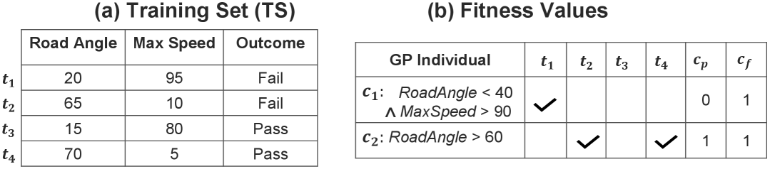
Figure 7: Computing $c_{p}(c)$ and $c_{f}(c)$ in SBFL fitness functions in Figure 6 for our GP-based condition inference.

SBFL functions assign high values to conditions met by many failing and few passing test inputs in the training set. By using SBFL ranking functions as fitness functions, our GP-based approach selects conditions that are more likely to explain and characterize failures effectively. For fitness functions that explain passing test cases, we swap $c_{f}$ with $c_{p}$ and swap $\mathit{TS}_{p}$ with $\mathit{TS}_{f}$ in the functions of Figure 6.

III-B Condition Inference by Interpretable ML

The second alternative we consider for generating conditions defined over the SUT’s input variables is interpretable ML. Specifically, we consider decision trees (DT) and decision rules (DR) as two forms of interpretable supervised ML models. Other interpretable supervised ML models such as linear, logistic, and polynomial regression assume linear or polynomial relations between the input variables and the test verdict [37]. Hence, these models are limited in their ability to capture the conditions required by our test oracles, which take the form of non-linear and rule-based constraints between input variables and test verdicts.

Inferring conditions using either DT or DR involves two steps: (1) Feature Engineering: We define input features for learning, initially using the system’s input variables as default features. However, if only these variables are used, DT and DR can learn only simple conditions that relate a single variable to a constant through a relational operator. For systems where the relationship between input variables and test outcomes is more complex, feature engineering becomes crucial. This process involves creating features that combine input variables using mathematical operators, allowing DT and DR to learn conditions based on these arithmetic combinations, similar to those generated by the grammar $\mathcal{G}$ in Figure 5. (2) Model Training and Condition Generation: With the input features established, we train the DT or DR models using the training set $\mathit{TS}$ generated in the first step of GenTC. DT and DR generate conditions as disjunctions of conjunctions of expressions that relate input features to constants, similar to conditions generated by the grammar $\mathcal{G}$. These models can produce conditions for both pass and fail verdicts.

III-C Test Oracle Building

In the third and final step, we construct consistent assertion-based test oracles from the conditions generated in the second step of GenTC. To do so, we first calculate each condition’s confidence level based on its precision in classifying pass or fail tests in the training set. Specifically, if condition $\mathit{cnd}$ is associated with a fail (or pass) verdict, its confidence level is the percentage of actual fail (or pass) test inputs in the training set that satisfy $\mathit{cnd}$, relative to all test inputs that satisfy $\mathit{cnd}$. For instance, if the condition $c_{2}$ in Figure 7 is associated with a pass verdict, its confidence level is $50\%$ because among the two tests in the training set that satisfy $c_{2}$ (i.e., $t_{2}$ and $t_{4}$), only $t_{4}$ has a pass verdict.

Then, we retain only those conditions whose confidence levels meet or exceed the user-defined verdict threshold $\theta$. Recall from Definition 3 that $\theta$ specifies the minimum confidence level required for a condition to be included in the assertion-based test oracle.

Next, we apply a pruning strategy to obtain a consistent set of assertions in the test oracle. Recall from Definition 2 that a consistent test oracle ensures no conflicting assertions exist, where one assertion indicates a test input passes while another indicates it fails. While DT-inferred assertions are consistent by construction, those inferred by GP or DR may require pruning to maintain consistency. Below, we first establish the necessary notation and definitions, and then describe our pruning strategy for obtaining a consistent set of assertions.

Definition 4 (Bipartite Graph based on Assertion Conditions).

Let $A$ be a set of assertions. We define the bipartite graph $\mathcal{B}=(V,E)$ corresponding to $A$ as follows: each assertion in $A$ corresponds uniquely to a vertex in $V$. The set $V$ is partitioned into two disjoint subsets $V_{p}$ and $V_{f}$, where $V_{p}$ represents conditions of the pass assertions in $A$, and $V_{f}$ represents conditions of the fail assertion in $A$. An edge $(x,y)\in E$ connects a vertex $x\in V_{p}$ to a vertex $y\in V_{f}$ if and only if the conjunction of their associated assertion conditions is satisfiable (SAT). More precisely, an edge between $x$ and $y$ indicates that the pair of assertions corresponding to $x$ and $y$ together represent an inconsistency within $A$ since they, respectively, represent a passing assertion and a failing assertion that can simultaneously hold for some test input.

Figure 8 shows a bipartite graph where $a_{1}$, $a_{2}$, $a_{3}$, and $a_{4}$ represent conditions of pass assertions (i.e., they belong to $V_{p}$), and $a^{\prime}_{1}$, $a^{\prime}_{2}$, and $a^{\prime}_{3}$ represent conditions of fail assertions (i.e., they belong to $V_{f}$). The edges in this graph represent pairs of pass and fail assertions whose conjunctions are satisfiable. For example, there is an edge between $a_{1}$ and $a^{\prime}_{1}$ because $x_{2}<43\wedge x_{1}+x_{2}<10$ is SAT.

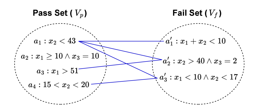
Figure 8: Pruning inconsistent assertions from test oracles using a bipartite graph representation. In this figure, $V_{p}$ denotes pass-class conditions, while $V_{f}$ denotes fail-class conditions.

Let $x\in V$ be a vertex. We denote the length of the condition associated with $x$ by $\mathit{len}(x)$, defined as the number of arithmetic and logical operators present in that condition. For example, in Figure 8, $\mathit{len}(a_{1})=1$ and $\mathit{len}(a_{2})=3$. We also denote the degree of a vertex $x$ by $\mathit{deg}(x)$, defined as the number of edges connected to $x$. For instance, in Figure 8, $\mathit{deg}(a_{1})$ is three, indicating that the passing assertion corresponding to $a_{1}$ is inconsistent with the failing assertions corresponding to $a^{\prime}_{1}$, $a^{\prime}_{2}$, and $a^{\prime}_{3}$.

We now present our pruning method, shown in Algorithm 2, which aims to eliminate inconsistencies (i.e., edges) between pass and fail conditions by removing vertices (i.e., conditions) from $V_{p}$ or $V_{f}$. Since there are multiple ways to eliminate inconsistencies, resulting in alternative consistent sets of assertions, we devise heuristics in Algorithm 2 whose goal is to obtain a consistent set of assertions while minimizing the number of removed vertices. Algorithm 2 takes a potentially inconsistent set of assertions $A$ and generates a consistent subset $A^{\prime}$ of assertions from $A$. Based on Definition 4, the algorithm represents $A$ as a bipartite graph $\mathcal{B}=(V,E)$, where each assertion condition becomes a vertex in $V$ and each satisfiable pass-fail pair is an edge in $E$ (line $1$ in Algorithm 2). We use the Z3 SMT solver [38] to check the satisfiability of the conjunctions of all pairs of pass and fail conditions to establish edges.

Algorithm 2 Pruning strategy to obtain a consistent set of assertions

Input $\mathit{A}$: A (potentially inconsistent) set of assertions
Output $A^{\prime}$: A consistent subset of $\mathit{A}$

1: Let $\mathcal{B}=(V,E)$ be a bipartite graph created based on Definition 4.

2: while $E\neq\emptyset$ do

3:  $S\leftarrow$ $\{x\in V\mid\mathit{deg(x)\geq 1\wedge\forall y\in V:\mathit{len(x)}\leq\mathit{len(y)}}\}$

4:  if $\mid S\mid\ ==1$

5:    $\mathit{vertextToRemove}\leftarrow$ select the vertex in $S$

6:  else

7:    $H\leftarrow$ $\{x\in S\mid\forall y\in S:\mathit{deg(x)}\geq\mathit{deg(y)}\}$

8:    if $\mid H\mid\ ==1$

9:      $\mathit{vertextToRemove}\leftarrow$ select the vertex in $H$

10:    elseif $H\cap V_{p}\neq\emptyset$

11:      $\mathit{vertextToRemove}\leftarrow$ randomly select a vertex in $H\cap V_{p}$

12:    else

13:      $\mathit{vertextToRemove}\leftarrow$ randomly select a vertex in $H$

14:    end

15:  end

16:  $V\leftarrow V\setminus\{\mathit{vertextToRemove}\}$

17:  $E\leftarrow E\setminus\{(u,v)\in E\mid u=\mathit{vertextToRemove}\vee v=\mathit{vertextToRemove}\}$

18: end

19: $A^{\prime}\leftarrow$ $\{x\Rightarrow\mathit{fail}\mid x\in V_{f}\}\cup\{x\Rightarrow\mathit{pass}\mid x\in V_{p}\}$

20: return $A^{\prime}$

In the while-loop from lines 2 to 18, Algorithm 2 iteratively removes vertices until there are no remaining edges between the pass ($V_{p}$) and fail ($V_{f}$) partitions. The loop begins by identifying the set $S$ of vertices with a degree of at least one and the shortest length among such vertices (line 3 in Algorithm 2). If $S$ contains exactly one vertex, that vertex is selected and stored in the variable vertexToRemove (lines 4–5 in Algorithm 2) for removal at the end of the while-loop iteration. This is because the condition corresponding to this vertex is the least constrained, thus having a higher likelihood of conflicting with other conditions, making it a priority candidate for removal.

If multiple vertices exist in $S$, the algorithm computes the subset $H\subseteq S$ containing vertices with the highest degree (line 7 in Algorithm 2). If $H$ contains exactly one vertex, this vertex is selected for removal (lines 8–9 in Algorithm 2). Otherwise, when multiple vertices exist in $H$, the algorithm prioritizes vertices belonging to the pass set ($V_{p}$) by randomly selecting one vertex in $H\cap V_{p}$ (lines 10–11 in Algorithm 2). This prioritization is motivated by the observation that the fail partition ($V_{f}$) typically contains fewer vertices, making fail vertices more valuable to retain. If no vertex in $H$ belongs to the pass set, the algorithm randomly selects a vertex from $H$ (line 13 in Algorithm 2). Having stored a vertex in vertexToRemove, this vertex and all its incident edges are removed from the graph (lines 16–17 in Algorithm 2). The assertions corresponding to the remaining vertices in $V_{p}$ and $V_{f}$ are collected into the set $A^{\prime}$, which is then returned (lines 19–20 in Algorithm 2).

Algorithm 2 ensures that the returned set $A^{\prime}$ is consistent. This is because at each iteration, the algorithm removes exactly one vertex with at least one incident edge. Since the graph $\mathcal{B}=(V,E)$ has a finite number of edges, the algorithm terminates after at most $|E|$ iterations. Upon termination, all edges – representing inconsistent pairs of assertion conditions – have been removed. Hence, the set $A^{\prime}$ is consistent.

For example, in Figure 8, vertex $a_{1}$ is removed first because it has the shortest condition and the highest degree. Next, $a_{3}$ is removed since it has the highest degree and a condition shorter than those of the vertices with the same degree, i.e., $a^{\prime}_{2}$, $a_{4}$ and $a^{\prime}_{3}$. Finally, $a_{4}$ is removed as it belongs to the pass class and has the same length and degree as $a^{\prime}_{3}$. After removing $a_{1}$, $a_{3}$ and $a_{4}$, the remaining conditions are consistent.

IV Assertion-based Test Oracles for Signal-based CPS

In this section, we adapt Definition 2 to signal-based CPS. While Definition 2 provides a notion of assertion-based test oracles for discrete-input CPS, signal-based CPS require a formulation that accounts for inputs expressed as signals – that is, functions over time. In this section, we present a running example to demonstrate assertion-based test oracles for CPS with signal inputs. We then explain how assertions are specified over these signals and characterize the expressiveness of such assertions in capturing signal properties.

IV-A Motivating Example from the CPS Domain

To demonstrate assertion-based test oracles for CPS with signal-based inputs, we introduce, as our running example, a simplified autopilot controller, referred to as Autopilot. Similar to most CPS, Autopilot operates on inputs represented as signals – functions defined over time. Specifically, Autopilot takes three primary inputs: throttle, which represents the engine power adjustment applied by the pilot; pitchwheel, which determines the degree of upward or downward tilt of the aircraft nose; and turnknob, which regulates the aircraft’s turn rate. Based on these input signals, Autopilot issues commands to the aircraft’s actuators to control the aircraft’s orientation and movement.

Autopilot has a requirement stating that the aircraft should reach a specified altitude within 500 seconds. A test input violating this requirement is considered a failure, whereas a test input meeting this requirement is deemed a pass. Determining whether a test passes or fails requires executing the Autopilot model with the given input values. However, test execution is time-consuming, as each run involves simulating Autopilot’s behaviour over a specified duration.

To reduce costs, we develop an assertion-based test oracle for Autopilot to determine test verdicts without the need to simulate the system. Figure 9 shows three assertions defined over Autopilot’s inputs: the pitchwheel signal (denoted by signal variable $p$), the turnknob signal (denoted by signal variable $k$), and the throttle signal (denoted by signal variable $th$). Further, the figure shows four test inputs ($t_{1}$ to $t_{4}$) for Autopilot, each displaying signals for throttle, pitchwheel, and turnknob. Using the assertions, we can determine verdicts for tests $t_{1}$ to $t_{4}$ without executing them. Specifically, the assertions in Figure 9 conclusively determine verdicts for three of the four tests. Hence, only one test input, i.e., $t_{3}$, for which a conclusive verdict cannot be produced, requires actual execution, rather than all four.

Note that these three signal variables, $p$, $k$, and $\mathit{th}$, are defined over time, and the assertions in Figure 9 constrain their values over time. Below, we describe how the assertions over the signal variables in Figure 9 are generated by grammar $\mathcal{G}$ in Figure 5.

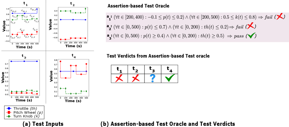
Figure 9: (a) An example set of test inputs for a (signal-based) autopilot system, with input signals $\mathit{Throttle}$, $\mathit{Pitch\ Wheel}$, and $\mathit{Turn\ Knob}$; (b) An assertion-based test oracle for this system. In this figure, ✓ denotes a pass verdict, ✗ denotes a fail verdict, and ? denotes an inconclusive verdict.

IV-B Assertions over Signals

Let $M$ be a CPS with input signals. We denote each test input for $M$ as $\bar{u}=\{u_{1},u_{2},\ldots,u_{m}\}$ where each $u_{i}$ is a signal for an input of $M$ over a time domain $\mathbb{T}=[0,b]$, i.e., $u_{i}:\mathbb{T}\rightarrow\mathbb{R}$. For example, each test input for the Autopilot example in Figure 9 represents the values for the three signals: $\mathit{th}$, $p$ and $k$, over the time domain $\mathbb{T}=[0,500s]$.

To generate signals, we use control-point encoding [39, 40] – a common approach in signal processing and control theory that captures signals in a compact and efficient representation. Specifically, we encode signals as sequences of equally spaced control points, where each index denotes a fixed time interval and each corresponding value approximates the signal’s value during that time interval. Following this encoding, to generate signals, it suffices to generate the control points of the signal. Provided with the control points, the actual signals are constructed through interpolation. An interpolation function (e.g., piecewise constant, linear, or cubic) connects the control points to form a signal [39, 40, 41]. In this article, we assume the interpolation function for system inputs is piecewise constant. Our evaluation of major CPS benchmarks and case studies from the literature indicates that most assume inputs to be piecewise constant. Notably, the Lockheed Martin industrial CPS benchmark and the MathWorks’ publicly available CPS models for automotive driving systems – including the cruise controller [22], clutch lockup controller [23], guidance control system [24], and DC motor controller [25] – explicitly use piecewise-constant input signals. In addition, the ARCH benchmark [26], which includes seven hybrid CPS models, compares two interpolation function types: arbitrary piecewise continuous functions and piecewise constant functions. Results from ARCH-COMP19 [42] show that performance differences between these two interpolation functions are minimal, indicating that our assumption of piecewise-constant signals is not restrictive.

Let $u:\mathbb{T}\rightarrow\mathbb{R}$ be an input signal. We encode $u$ using $n_{u}$ control points, i.e., $c_{u,0}$, $c_{u,1}$, …, $c_{u,n_{u}-1}$, equally distributed over the time domain $\mathbb{T}=[0,b]$, i.e., positioned at a fixed time distance $I=\frac{b}{n_{u}-1}$. Let $c_{x,y}$ be a control point, $x$ is the signal the control point refers to, and $y$ is the position of the control point. The control points $c_{u,0}$, $c_{u,1}$, …, $c_{u,n_{u}-1}$ respectively contain the values of the signal $u$ at time instants $0,I,2\cdot I,\ldots,(n_{u}-1)\cdot I$. For example, in the test inputs in Figure 9, pitchwheel (denoted by $p$) and turnknob (denoted by $k$) are represented using six control points (denoted by $c_{p,0},\ldots,c_{p,5}$ for the pitchwheel and $c_{k,0},\ldots,c_{k,5}$ for the turnknob), while throttle (denoted $\mathit{th}$) is represented using three control points (denoted by $c_{th,0},\ldots,c_{th,2}$) over the $[0,500s]$ time domain.

Assertion conditions over signals are generated according to the syntactic rules of grammar $\mathcal{G}$ in Figure 5 by using cp to represent signal control points. Furthermore, to ensure the well-formedness of the conditions, we constrain each arithmetic expression, exp, to contain only signal control points at the same position. For example, the condition $(c_{k,0}-c_{p,0}\geq 0)\;\land\;(c_{k,1}+c_{th,1}<1)$ can be generated by our grammar and satisfies the constraint that each arithmetic expression must involve control points associated with the same position; $c_{k,0}$ and $c_{p,0}$ in the first expression are control points at position 0, and $c_{k,1}$ and $c_{th,1}$ in the second expression are control points at position 1.

IV-C Expressive Power of Assertions over Signals

We now discuss the expressive power of the assertions generated using grammar $\mathcal{G}$ in Figure 5 over signal control points. To do so, we first present a translation of assertion conditions defined over control points into constraints defined over signal variables directly. Our translation consists of two sets of rewriting rules: The first set of rewriting rules, based on Menghi et al. [21], introduces a $\forall$ quantifier over each arithmetic expression, exp, while replacing signal control points with signal variables in these expressions. The second set of rules consists of standard logic rewriting rules: one for merging universal quantifiers over disjoint domains, and another for conjunction of universal quantifiers over the same domain.

Rules for replacing signal control points with signal variables [21]. Let $u:\mathbb{T}\rightarrow\mathbb{R}$ be an input signal. Suppose we represent $u$ using the following $n_{u}$ control points: $c_{u,0}$, $c_{u,1}$, …, $c_{u,n_{u}-2}$, $c_{u,n_{u}-1}$ such that each control point $c_{u,i}$ is positioned at position $i\cdot I$ where $I=\frac{b}{n_{u}-1}$. Let exp be an arithmetic expression generated by the grammar $\mathcal{G}$ in Figure 5. Based on the definition of assertions over signals given above, exp contains only signal control points in the same position $j$. This expression can then be rewritten into the following equivalent logical expression $\forall t\in[j\cdot I,(j+1)\cdot I):\texttt{exp}^{\prime}$ where $\texttt{exp}^{\prime}$ is obtained by substituting each control point $c_{u,j}$ with the expression $u(t)$ representing the input signal $u$ at time $t$. Note that this rewriting rule is valid because we assume that the interpolation function connecting the control points is piecewise constant.

For example, in Figure 9, consider the control points $c_{k,0}$ to $c_{k,5}$ for the turnknob signal $k$, and the control points $c_{p,0}$ to $c_{p,5}$ for the pitchwheel signal $p$. The first control point of both signals is at time 0s, the second at 100s, the third at 200s, and so on. Now, consider the following condition over these control points which can be generated by our grammar:

$(c_{k,0}-c_{p,0}\leq 20)\wedge(c_{k,1}+c_{p,1}<0)$

The above condition is rewritten into the following logical formula over turnknob ($k$) and pitchwheel ($p$) signals based on the rule discussed above:

$(\forall t\in[0,100):k(t)-p(t)\leq 20)$  $\wedge$ $(\forall t\in[100,200):k(t)+p(t)<0)$

Note that for the control points at position zero, i.e., $c_{k,0}$ and $c_{p,0}$, we quantify the variable $t$ over the domain $[0,100)$, and for the control points at position one, i.e., $c_{k,1}$ and $c_{p,1}$, we quantify the variable $t$ over the next time slot $[100,200)$.

Quantifier conjunction rules. After introducing universal quantifiers and replacing control points with signal variables, we apply the following standard logic rewriting rules:

$$\begin{array}[]{l}\left(\forall t\in A:\texttt{exp}\right)\land\left(\forall t\in B:\texttt{exp}\right)\ \equiv\ \forall t\in A\cup B:\texttt{exp}\\ \left(\forall t\in A:\texttt{exp}\right)\land\left(\forall t\in A:\texttt{exp}^{\prime}\right)\ \equiv\ \forall t\in A:\texttt{exp}\land\texttt{exp}^{\prime}\end{array}$$

where exp and $\texttt{exp}^{\prime}$ are arithmetic expressions containing signals over the time domain $\mathbb{T}=[0,b]$, and $A$ and $B$ are two time domains that are subsets of $\mathbb{T}$.

Figure 10 illustrates the condition assertions generated using our grammar over the control points of the turnknob ($k$), pitchwheel ($p$), and throttle ($\mathit{th}$) signals, along with the step-by-step translation of these conditions into logical formulas over their corresponding signal variables. For example, in Figure 10(b), the condition
$c_{p,0}\leq 0.7\land c_{p,1}\leq 0.7\land c_{p,2}\leq 0.7\land c_{p,3}\leq 0.7\land c_{p,4}\leq 0.7\land c_{th,0}\leq 0.2$
is converted into the logical formula:
$(\forall t\in[0,500):p(t)\leq 0.7)\land(\forall t\in[0,200):th(t)\leq 0.2)$.
To perform this translation, we first rewrite each relational term (e.g., $c_{p,0}\leq 0.7$) in the condition into its logical equivalent using the rule $\mathit{exp}\rightarrow\forall t\in[j.I,(j+1).I]:\mathit{exp^{\prime}}$ where $j$ is the position of the control point and $I$ is the sampling interval. We then apply the quantifier conjunction rules to combine the resulting quantified expressions into a single statement that covers the union of their time ranges.

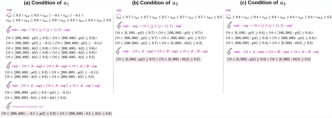
Figure 10: Step-by-step illustration of using rules to derive logical assertion conditions over the signals in Figure 9 from assertion conditions based on the control points of turnknob ($k$), pitchwheel ($p$) and throttle ($th$).

Having provided the rewriting rules above, we can now discuss the expressiveness of the conditions obtained after applying the rewriting rules. Let $\bar{u}={u_{1},\ldots,u_{m}}$ be signals over $\mathbb{T}$, and let $T=\{t_{1},\ldots,t_{d}\}$ be a set of time variables. Suppose we generate conditions over the control points of the signals in $\bar{u}$ using grammar $\mathcal{G}$ in Figure 5. After applying the two rewriting rule sets above, the generated formulas are expressible within the following logic fragment, denoted by $\mathcal{L}$:

$$\psi\Coloneqq \psi_{1}\vee\psi_{2}\mid\phi$$

$$\phi\Coloneqq \rho\sim 0\mid\phi_{1}\wedge\phi_{2}\mid\forall t\in\langle n_{1},n_{2}\rangle\colon\phi$$

$$\rho\Coloneqq u(t)\mid r\mid\rho_{1}+\rho_{2}\mid\rho_{1}-\rho_{2}\mid\rho_{1}\times\rho_{2}\mid\rho_{1}/\rho_{2}$$

where $n_{1},n_{2}$ are non-negative real numbers including zero, $r\in\mathbb{R}$, $t\in\mathbb{T}$, $u\in\bar{u}$, $\sim$ is a relational operator in $\{<,\leq,>,\geq,=,\neq\}$, and $\langle n_{1},n_{2}\rangle$ is a time interval of $\mathbb{T}$ (i.e., $\langle n_{1},n_{2}\rangle\subseteq\mathbb{T}$). The symbols $\langle$ and $\rangle$ are equal to $[$ or $($, respectively to $]$ or $)$, depending on whether $n_{1}$, respectively $n_{2}$, are included or excluded from the interval.

We argue that any condition obtained by our grammar $\mathcal{G}$ and modified through our rewriting rules is a formula in $\mathcal{L}$. Conversely, any formula $\varphi\in\mathcal{L}$ that satisfies the following two conditions corresponds to a condition that can be generated by the grammar $\mathcal{G}$: (1) $\varphi$ is closed, i.e., does not contain any free occurrence of the variable $t$, and (2) $\varphi$ does not involve any nested use of the $\forall$ quantifier.

The argument follows by structural induction and noting that the nonterminal $\psi$ in $\mathcal{L}$ corresponds to or-term in $\mathcal{G}$; the nonterminal $\phi$ in $\mathcal{L}$ corresponds to and-term in $\mathcal{G}$; $\rho\sim 0$ in $\mathcal{L}$ maps to rel-term in $\mathcal{G}$; the nonterminal $\rho$ in $\mathcal{L}$ maps to the nonterminal exp in $\mathcal{G}$; and terminal $r$ in $\mathcal{L}$ maps to const, and terminal $u(t)$ in $\mathcal{L}$ maps to cp in $\mathcal{G}$. The complete proof is in Appendix A.

Comparing $\mathcal{L}$ with Signal Temporal Logic (STL) [19], the logic $\mathcal{L}$ is able to express the temporal operator globally, i.e., $G$, from STL. Specifically, the STL property

$$G_{[0,500)}(\mathit{th}(t)<100)$$

i.e., the throttle should remain less that $100$ from 0s to 500s, corresponding to the following formula in $\mathcal{L}$:

$$\forall t\in[0,500):(\mathit{th}(t)<100)$$

which corresponds to the following condition generated by the grammar $\mathcal{G}$ utilizing control points $c_{th,0}$, $c_{th,1}$, and $c_{th,2}$:

$$c_{th,0}<100\wedge c_{th,1}<100\wedge c_{th,2}<100$$

In addition, $\mathcal{L}$ can express arithmetic operations within predicates, which are not part of the core STL formula syntax, thus extending STL with explicit arithmetic expression support. Specifically the following formula in $\mathcal{L}$, $(\forall t\in[0,100):k(t)-p(t)\leq 20)$ cannot be directly specified in STL, as STL does not include arithmetic operators in its core syntax.

To demonstrate that $\mathcal{L}$ is capable of expressing common CPS properties, we assessed a dataset of 98 industrial CPS requirements previously used by Menghi et al. [21]. Menghi et al. formalized this dataset in restricted signal first-order logic, a logic fragment proposed in their study. Of the 98 formalized requirements, 85 can be expressed in our logic $\mathcal{L}$. The remaining 13 cannot, as they rely on existential quantifiers ($\exists$) or nested universal quantifiers ($\forall$), which lie outside the scope of $\mathcal{L}$. The fact that $86$% of the industrial CPS requirements can be expressed in $\mathcal{L}$ demonstrates that the logic fragment $\mathcal{L}$ remains highly expressive for capturing a wide range of real-world CPS properties. In our replication package [27], we have included the $85$ natural-language requirements along with their corresponding formalizations.

V Evaluation

In this section, we evaluate GenTC using case studies from the CPS domain. Our case studies involve simulators and testbeds that are prone to flakiness, leading to potential variations in the datasets used to infer test oracles. We assess the accuracy of test oracles generated using the alternative condition-inference techniques described in Sections III-A and III-B. We further examine the impact of training-set variations, caused by the SUT’s flakiness, on the accuracy and robustness of the generated test oracles.

Our evaluation starts with RQ1, which assesses the extent of flakiness in the test results from our case-study systems. The goal is to confirm the presence of flakiness in these systems and to estimate its prevalence. In RQ2, we evaluate the accuracy and effectiveness of test oracles generated by the alternative condition-inference techniques in Sections III-A and III-B. In RQ3, we evaluate whether flakiness in the training sets affects the accuracy of test oracles. When the SUT is flaky, re-running tests can produce different verdicts. Ideally, the generated test oracles should remain robust, regardless of which run of the system the training set is derived from.

RQ1 (Existence of Flakiness) How flaky are our case-study systems? We assess the level of flakiness in our network, ADS and aerospace case studies by calculating the percentage of inconsistent test verdicts from multiple re-executions of randomly selected test inputs.

RQ2 (Accuracy) How accurate are the assertion-based test oracles inferred by our approach using different condition-inference methods? We examine the accuracy of the assertion-based test oracles generated by the alternative condition-inference techniques described in Sections III-A and III-B.

RQ3 (Robustness to Flakiness) How is the accuracy of test oracle assertions impacted when using training sets from different executions of the SUT? We study the robustness of our assertion-generation technique as a way to ensure that its accuracy is not significantly affected when using training sets from different executions of the SUT.

V-A Study Subjects

We use five network, aerospace and ADS systems as detailed below:

Router system. Our first case-study system is a router optimized for real-time streaming applications, such as video conferencing and online meetings. The router uses priority-based flow management, dividing the incoming traffic into different priority classes. The router’s real-world deployment involves both hardware and software. We evaluate this router using an open-source virtual testbed we have developed in our earlier work [43], which accurately simulates the router’s operational environment, allowing for large-scale, high-fidelity experimentation. The inputs to the router are bandwidths of data flows passing through the router’s priority classes. To ensure realism in our experiments, we ensure that the total bandwidth of data flows does not exceed the system’s capacity. Further, we consider different traffic profiles – for example, small, frequent UDP packets for VoIP traffic, and larger, bursty TCP flows for background traffic such as file transfers. The router testbed enables us to assess whether the user experience for streaming services is satisfactory (pass) or unsatisfactory (fail). Each test execution takes approximately $4.5$ minutes and is compute-intensive. In addition, there is non-determinism in the test results due to fluctuations in network bandwidth, latency, jitter, asynchrony in network flows, and the CPU and memory load on the machine hosting the testbed.

Aircraft autopilot system. We use an autopilot model of a De Havilland Beaver aircraft derived from a public-domain benchmark of Simulink specifications provided by Lockheed Martin [20]. Simulink [44] is a widely used language for CPS specification and simulation. An example based on this system, simplified to have fewer inputs, is illustrated in Section IV-A. The Simulink model of autopilot captures both the autopilot system, which includes the control logic and algorithms responsible for stabilizing and navigating the aircraft, as well as the simulator, which simulates the aircraft’s physical dynamics and environmental factors such as wind and turbulence. The inputs to the autopilot system are signals related to the flight dynamics of the aircraft such as throttle, pitch angle, turning rate, heading and desired flight objectives such as a target altitude. We encode these signals using control points and apply piecewise interpolation to connect the control points. To ensure realism in our experiments, we avoid abrupt or conflicting changes in signals such as throttle and pitch angle that would violate aircraft dynamics. The autopilot system is expected to satisfy the following system-level requirement: when the autopilot is enabled, the aircraft should reach the desired altitude within $500$ seconds in calm air.

The publicly available Simulink model of the autopilot system, provided by MathWorks, is developed in compliance with the DO-178C standard [45, 46], which requires the software to respond predictably to the same inputs and conditions. Consequently, in this Simulink model, the gust amplitude and direction – despite being inherently stochastic – are fixed to specific values. Furthermore, the turbulence model uses fixed noise seeds to eliminate non-determinism. Thus, while the system’s design incorporates stochastic elements, the publicly available model is intentionally made deterministic. In our experiments, we used this deterministic Simulink model of the autopilot system. The autopilot case study – while deterministic and thus not susceptible to flakiness as also shown in RQ1 – nonetheless involves complex signal-based inputs, making it an interesting system for evaluating the accuracy of the assertion-based test oracle in RQ2.

ADS systems. We use two types of self-driving controllers as our ADS systems, both executed and tested using the BeamNG simulator – a widely used open-source tool for ADS testing [47]. The first system is the autopilot controller of BeamNG, a classical self-driving controller [47, 48]. The second is Dave2 [49], a deep neural network (DNN) model trained for end-to-end self-driving. To test the autopilot controller, we developed two simulation environments in BeamNG: (1) a complex town map with multi-lane roads, other vehicles, and various static objects along the roads, and (2) a simpler environment with a two-lane road without other vehicles and static objects. We refer to the setup that tests the autopilot controller on the town map as AP–TWN, and the one testing it on the simpler road as AP–SNG. We test Dave2 using only the simpler road map, as Dave2 is specifically trained for this environment. The inputs to AP–SNG and Dave2 include road shape, weather conditions, time of day, the initial and target positions of the ego vehicle, as well as its speed and type. In addition to these, AP–TWN also takes as input the number of non-ego vehicles in the map, along with the initial and target positions, speeds, and types of both ego and non-ego vehicles. To ensure realism in our experiments, we enforce plausible vehicle positions, feasible target positions and avoid initial collisions caused by physically implausible starting positions or unsafe spacing between vehicles. The Dave2 model and the single road setup used in our evaluation are provided by the CPS Testing Tool Competition track at the SBFT workshop [50].

To determine whether a test passes or fails in our ADS setups, we consider the following system-level requirements adopted from prior studies [51, 50, 52]: For AP–SNG and Dave2, tested in the single-road environment, a test fails if the ego vehicle veers off the lane (R1). In the case of AP–TWN, operating in the complex town map, a test can fail not only for veering off the main road (R1) but also for three additional reasons: failing to maintain a safe distance from other vehicles (R2), failing to maintain a safe distance from static objects (R3), and not reaching the specified destination within the simulation duration (R4). Test execution time is approximately three minutes for AP–TWN and one minute for AP–SNG and Dave2. Flakiness in these ADS test setups can arise due to inconsistencies in timing between the simulator and ADS controller, which may lead to variations in the images or sensory data received by the ADS. Furthermore, the addition of white noise to the images passed to the ADS may contribute to flakiness [51]. In the more complex town map, factors like the presence of non-ego vehicles and traffic lights introduce additional flakiness in the test outcomes for AP–TWN.

Table I outlines the key characteristics of our study subjects. These subjects include the Router system, the aircraft autopilot (AP–DHB), the ADS autopilot controller tested in a complete town (AP–TWN) and on a single-road map (AP–SNG), as well as the DNN-based controller tested on a single-road map (Dave2). For AP–TWN, tested against the above-mentioned requirements (R1–R4), we present the results for each requirement separately.

TABLE I: Key characteristics of our case-study systems. System refers to the SUT along with the naming convention we adopt in the article. Simulator indicates the environment or testbed used for test execution and Test Execution Time indicates the approximate duration required to run a single test input on the corresponding simulator.

System	Simulator	Test Execution Time
Router [43]	Router Testbed	$\sim 4.5$ min
Aircraft autopilot system of De Havilland Beaver aircraft (AP–DHB) [46]	Simulink models of environmental factors (e.g., wind, turbulence, temperature, and atmospheric conditions) and aircraft’s physical dynamics	$\sim 0.5$ min
ADS autopilot tested in a complete town (AP–TWN)	BeamNG	$\sim 3$ min
ADS autopilot tested on a single road map (AP–SNG)		$\sim 1$ min
DNN self-driving controller tested on a single road map (Dave2)

V-B RQ1 (Existence of Flakiness)

Experiment setting. RQ1 measures the degree of flakiness in our case studies, namely the Router, AP–TWN, AP–SNG, Dave2, and AP-DHB. We randomly generate 100 test inputs for the router case study and 200 test inputs for each of our ADS-based and aerospace case studies. Since the router is our most resource-intensive system to execute, we generate a smaller number of test inputs for it. Each test input is executed 10 times to detect any non-determinism in the test outcomes. We then prepare ten datasets for each case study where each dataset contains the verdicts from a distinct execution of test inputs. We refer to each dataset as $\mathit{TS}_{n}$ where $n$ denotes the $n$-th execution of the test inputs. Consequently, for each case study, we obtain datasets $\mathit{TS}_{1}$, $\mathit{TS}_{2}$, $\ldots$, $\mathit{TS}_{10}$.

Results. Table II shows the percentage of flaky tests observed for each case study across $\mathit{TS}_{1}$ to $\mathit{TS}_{10}$. We consider a test case to be flaky unless all ten runs produce the same outcome. The percentage of flaky tests for AP–DHB is $0\%$, indicating the absence of flakiness in this system. In contrast, the percentage of flaky tests for Router is $11\%$. The percentage of flakiness for the tests exercising AP–TWN for requirements R1 to R4 ranges between $21\%$ and $79\%$.

TABLE II: Percentage of flaky tests in the systems of Table I

Router	AP–DHB	AP–TWN				AP–SNG	Dave2
		R1	R2	R3	R4
11%	0%	79%	64%	70%	21%	1.5 %	33%

V-C RQ2 (Accuracy)

Experiment setting. To answer RQ2, we generate test oracles using the GP, DT, and DR alternatives by applying these methods to the training sets for each case study. Specifically, for each case study, we select one of the ten datasets from RQ1 to serve as the training set. This enables us to assess each method without regard to the variations caused by flakiness across the different datasets from RQ1. Analyzing the impact of the variations caused by flakiness is left for RQ3. We tune the hyper-parameters of DT and DR using Bayesian Optimization [53]. We configure GP using the parameters in Table III and apply GP with each of the fitness functions from Figure 6: Naish denoted by $\mathit{GP_{N}}$, Tarantula denoted by $\mathit{GP_{T}}$, and Ochiai denoted by $\mathit{GP_{O}}$. To account for the randomness of GP, DT, and DR, we apply each technique 20 times to the training set for each case study.

In addition to considering the test oracle generation methods individually, we also consider an ensemble approach. Specifically, for each run of $\mathit{GP_{N}}$, $\mathit{GP_{T}}$, $\mathit{GP_{O}}$, DT, and DR, the ensemble method computes the union of the conditions generated by these techniques. Then, we derive a consistent set of assertions by applying the third step of GenTC (Section III-C) to this union. We then compare the assertion-based test oracles generated by the ensemble with those generated by each method individually.

Recall from Definition 3 that each SUT is associated with a user-defined verdict threshold $\theta$, which specifies the minimum confidence level required for an assertion to be included in the test oracle. We vary the user-defined verdict threshold $\theta$, from $0.5$ to $1$ in increments of $0.05$. We do not consider $\theta<0.5$, since verdict predictions by assertions with less than $50\%$ confidence are unlikely to be trusted and used in practice. In Section VI, we present actionable guidelines derived from our empirical analysis to select an optimal verdict threshold.

TABLE III: Parameters of GP: mutation rate (Mut_rate), crossover rate (Cr_rate), population size (Pop_size), number of generations (Num_gen), max. tree depth (Max_d), tournament size (T_size), split Criterion (Criterion), split strategy (Splitter), min. samples to split a node (Min_split), min. samples per leaf (Min_sample)

Parameter	Value	Parameter	Value	Parameter	Value	Parameter	Value
							ADS: 100
Mut_rate	0.1	Num_gen	50	Pop_size	50	Max_const	Router: 400
							Autopilot: 45
Cr_rate	0.7	T_size	7	Max_d	5	Min_const	ADS: 0
							Router: 0
							Autopilot: -30

Note: The values within the framed box 00 are from [32, 31, 54]. The values within the framed box 00 are set by assessing the average number of generations required to reach a plateau. The values within the framed box 00 are based on the lowest and highest values that the input variables of our systems can assume.

We generate each case study’s test set by randomly creating inputs and executing them on the case-study system to obtain ground-truth verdicts. To mitigate the impact of flaky behaviour on the ground-truth verdicts for test sets, we do as follows:

• For systems with a flaky test rate below 50%, we include only tests that exhibit consistent behaviour in all ten runs. Any test that shows flakiness in those runs is excluded from the test set.

• For systems with a flaky test rate above $50\%$, since completely excluding flaky tests is cost-prohibitive, we include tests that produce consistent verdicts in at least eight out of ten runs. Their final verdicts are determined by majority voting.

We ensure that each test set for each case study ultimately contained $200$ elements.

Results. To answer RQ2, we assess the accuracy of the generated test oracles using the metrics from Section II-C: accuracy, misprediction rates – i.e., the rate of pass verdicts predicted as fail, and the rate of fail verdicts predicted as pass – and relative accuracy. In addition to these metrics, we compare the test oracle generation methods based on the percentage of unique correct predictions. Specifically, given a pair of methods $A$ and $B$ and a test set $\mathit{TestSet}$, the percentage of unique correct predictions for method $A$ is the percentage of tests in $\mathit{TestSet}$ whose verdicts are correctly predicted by $A$ but not by $B$. Figure 11 illustrates using a Venn diagram notation the percentage of unique correct predictions for methods $A$ and $B$ as the “only $A$” and “only $B$” areas, respectively. The percentage of unique correct predictions indicates how well a method complements other methods. Below, we assess different test oracle generation methods using accuracy, misprediction rates, relative accuracy, and the percentage of unique correct predictions.

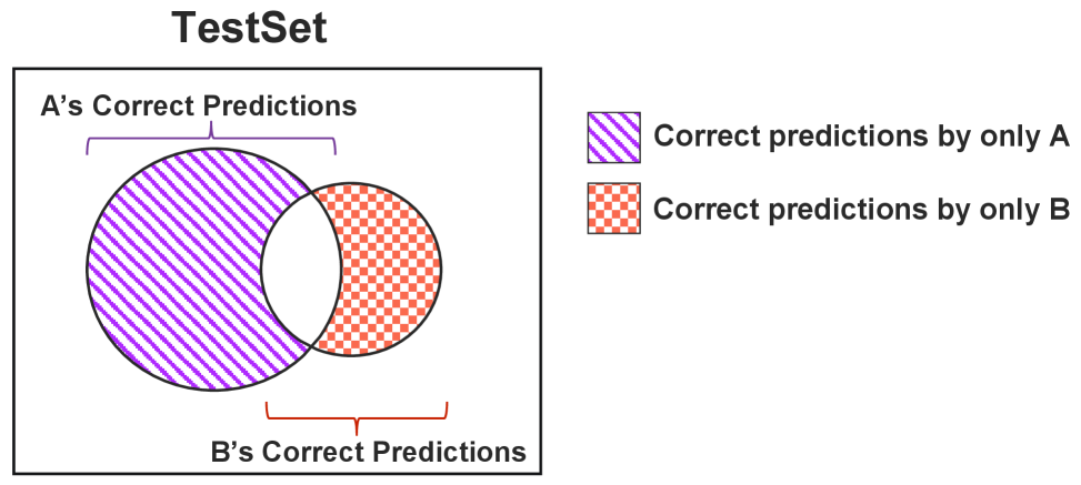
Figure 11: Illustrations of the percentage of unique correct predictions on a $\mathit{TestSet}$ made by methods A and B

All statistical tests are performed using the Mann-Whitney U test [55] and the Vargha-Delaney’s $\hat{A}_{12}$ effect size [56]. All statistical significance tests in RQ2 are reported with p-values adjusted using the Benjamini–Hochberg (BH) procedure [57]. We classify effect size values for accuracy and relative accuracy, where higher values indicate better performance, as follows: effect sizes are classified as small, medium, and large when their values are greater than or equal to 0.56, 0.64, and 0.71, respectively [56]. For misprediction rates, where lower values indicate better performance, effect sizes are classified as small, medium, and large when their values are lower than or equal to 0.44, 0.36, and 0.29, respectively [56].

(1) Accuracy. Figure 12 shows the average accuracy of the test oracles generated by each technique for all case studies when $\theta$ varies from $0.5$ to $1$. The average accuracy of test oracles generated by $\mathit{GP_{T}}$, $\mathit{GP_{O}}$, $\mathit{GP_{N}}$ and ensemble decreases as $\theta$ increases because a higher value of $\theta$ results in fewer assertions in these test oracles, as we only retain those with a confidence level of at least $\theta$. In contrast, since the confidence levels of assertions produced by DT and DR are generally high (i.e., above $0.8$), the accuracy of DT and DR remains relatively stable as $\theta$ increases.

For $0.5\leq\theta\leq 0.85$, $\mathit{GP_{O}}$ produces most accurate test oracles compared to other techniques. Statistical tests comparing the accuracy results in Figure 12 are provided in Table IX in the Appendix B. Based this table, for $0.5\leq\theta\leq 0.85$, test oracles generated by $\mathit{GP_{O}}$ are significantly more accurate than those generated by other techniques. The effect-size values for the comparisons of $\mathit{GP_{O}}$ with $\mathit{GP_{T}}$, DT, DR, and the ensemble are all large, while the comparisons of $\mathit{GP_{O}}$ with $\mathit{GP_{N}}$ show both large and small effect sizes. For $\theta\geq 0.9$, there are no statistically significant differences in accuracy between $\mathit{GP_{O}}$ and $\mathit{GP_{N}}$, DT or the ensemble method.

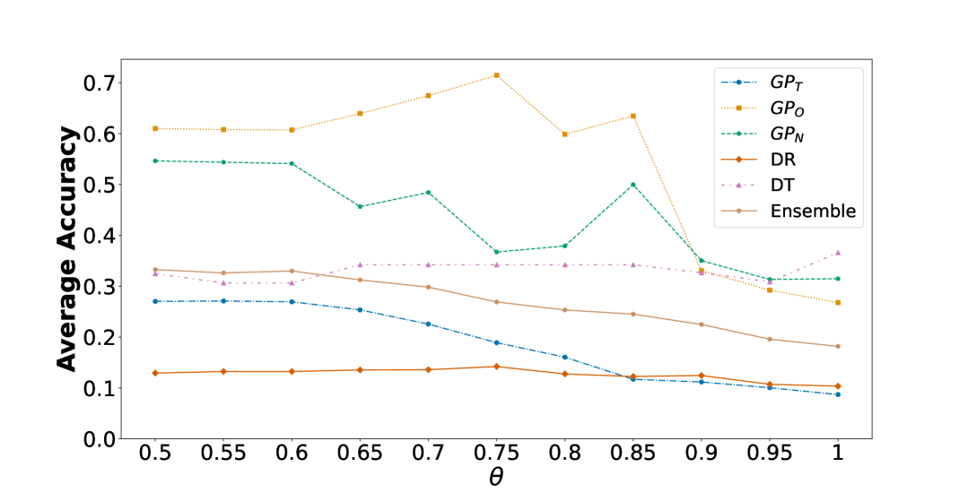
Figure 12: Average accuracies of the test oracles generated by $\mathit{GP_{T}}$, $\mathit{GP_{O}}$, $\mathit{GP_{N}}$, DT, DR and ensemble for all case studies when the verdict threshold $\theta$ varies from $0.5$ to $1$.

Statistical tests comparing the accuracy results of $\mathit{GP_{O}}$ with $\mathit{GP_{T}}$, $\mathit{GP_{N}}$, DT, DR, and the ensemble for each study subject across all values of $\theta$ are provided in Table X in Appendix B. Based on these results, test oracles from $\mathit{GP_{O}}$ are significantly more accurate than those from $\mathit{GP_{T}}$ and DR in all eight subjects, outperform ensemble in seven, DT in six, and $\mathit{GP_{N}}$ in five of the eight case studies. The effect size values for these comparisons are small, medium and large.

For AP–TWN (R4), test oracles generated by DT fail to predict any verdicts across all values of $\theta$. This is shown in Table X by stating DT is not applicable and highlighting the corresponding cells in yellow. We do not show the comparisons of $\mathit{GP_{T}}$, $\mathit{GP_{N}}$, DT, DR and ensemble with each method, as these comparisons provide no additional insights beyond Figure 12 and Tables IX and X. Full comparisons are available in our supplementary material [27].

(2) Misprediction Rates. Figures 13 and 14 show the rate of actual pass verdicts predicted as fail, and the rate of actual fail verdicts predicted as pass, respectively, for all case studies when $\theta$ varies from $0.5$ to $1$. For clarity, we report these two rates across the following three aggregated $\theta$-ranges, since presenting them for each individual $\theta$ does not provide a concise overview: low ($0.5\leq\theta<0.7$), medium ($0.7\leq\theta<0.9$), and high ($0.9\leq\theta$). We refer to the rate of pass verdicts predicted as fail as Pass-as-Fail, and the rate of fail verdicts predicted as pass as Fail-as-Pass.

As shown in Figure 13, across all $\theta$ ranges, DR consistently achieves the lowest (best) average Pass-as-Fail rates compared to all GP techniques – $\mathit{GP_{T}}$, $\mathit{GP_{O}}$, and $\mathit{GP_{N}}$ – as well as the ensemble and DT. In contrast, for the Fail-as-Pass misprediction results, the GP techniques overall, and in particular $\mathit{GP_{O}}$, produce better results compared to DT, DR, and the ensemble. Statistical tests comparing the Pass-as-Fail (Figure 13) and Fail-as-Pass (Figure 14) results are provided in Tables XI(a) and (b), respectively, in Appendix B. Specifically, for the Pass-as-Fail rate, we compare the best-performing method for this metric, DR, with the other techniques, and for the Fail-as-Pass rate, we compare its best-performing method, $\mathit{GP_{O}}$, with the others. Based on Table XI(a), test oracles generated by DR lead to a significantly lower rate of Pass-as-Fail compared to those obtained by other techniques with small, medium and large effect sizes. Based on Table XI(b) for $0.5\leq\theta<0.9$, $\mathit{GP_{O}}$ either achieves a significantly lower Fail-as-Pass rate (with small, medium and large effect sizes) or shows no statistically significant difference in Fail-as-Pass rate compared to other techniques. For $0.9\leq\theta\leq 1$, $\mathit{GP_{T}}$ results in a significantly lower Fail-as-Pass rate compared to other techniques.

Table XII in Appendix B presents the statistical tests comparing the Pass-as-Fail rate of DR and the Fail-as-Pass rate of $\mathit{GP_{O}}$ with those of the other techniques, for each study subject and across all values of $\theta$. Based on Table XII(a), test oracles generated by DR have a significantly lower Pass-as-Fail rate than those obtained by $\mathit{GP_{N}}$ in all eight study subjects, by $\mathit{GP_{T}}$ and $\mathit{GP_{O}}$ in seven, by ensemble in six, and by DT in four out of eight study subjects. Based on Table XII(b), test oracles generated by $\mathit{GP_{O}}$ have a significantly lower Fail-as-Pass rate than those obtained by DR in five study subjects, and by $\mathit{GP_{T}}$ and ensemble in four study subjects. The effect size values in all the comparisons are negligible, small, medium and large.

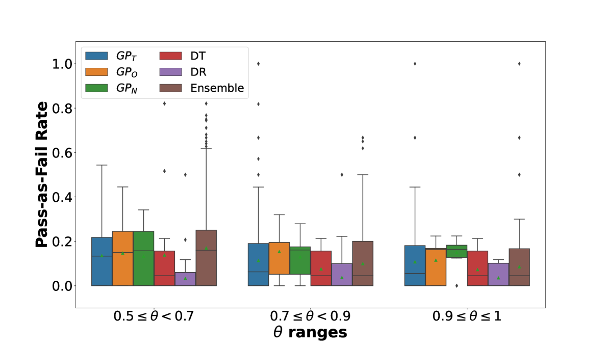
Figure 13: Pass-as-Fail rates of the test oracles generated by $\mathit{GP_{T}}$, $\mathit{GP_{O}}$, $\mathit{GP_{N}}$, DT, DR and ensemble for all case studies when the verdict threshold $\theta$ varies from $0.5$ to $1$.

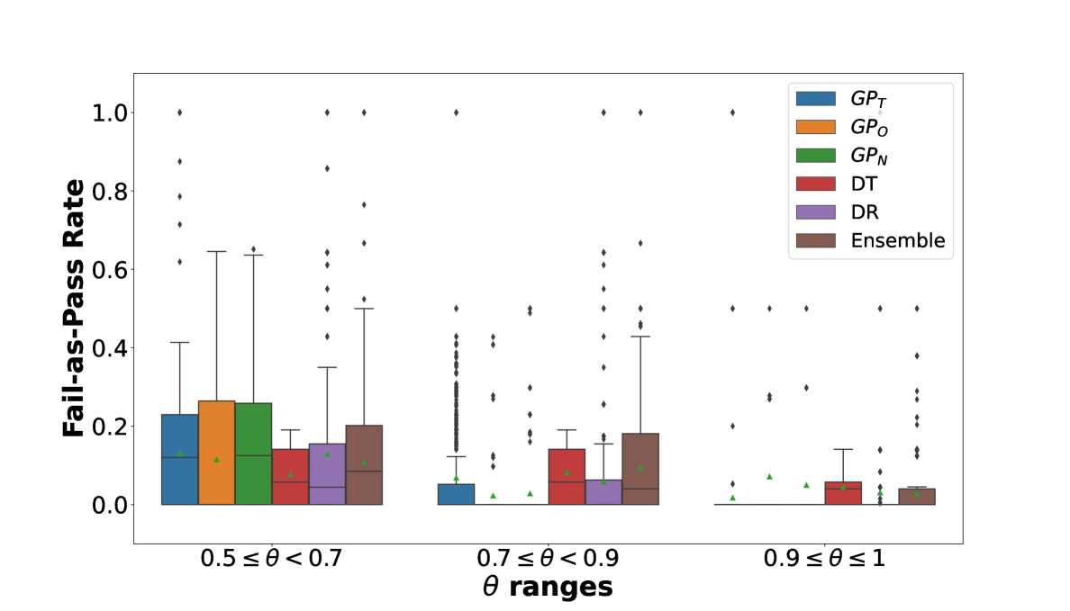
Figure 14: Fail-as-Pass rates of the test oracles generated by $\mathit{GP_{T}}$, $\mathit{GP_{O}}$, $\mathit{GP_{N}}$, DT, DR and ensemble for all case studies when the verdict threshold $\theta$ varies from $0.5$ to $1$.

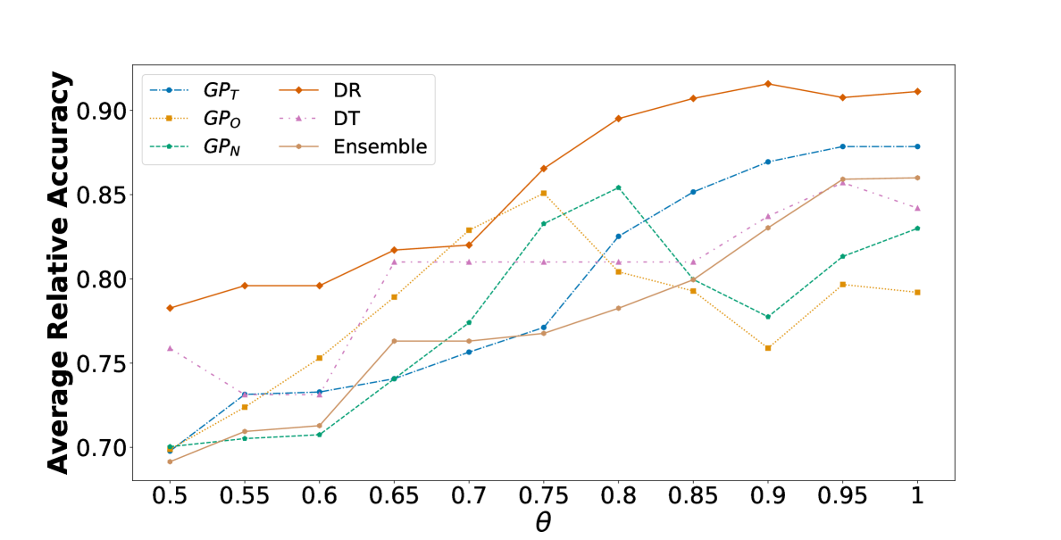
Figure 15: Average relative accuracies of the test oracles generated by $\mathit{GP_{T}}$, $\mathit{GP_{O}}$, $\mathit{GP_{N}}$, DT, DR and ensemble for all case studies when the verdict threshold $\theta$ varies from $0.5$ to $1$.

(3) Relative Accuracy. Figure 15 presents the average relative accuracy of the test oracles generated by GP, DT, DR and ensemble for all our case studies and for $0.5\leq\theta\leq 1$. Recall from Section IV that while accuracy is the percentage of correct predictions among all predictions, relative accuracy is the percentage of correct predictions excluding inconclusive predictions. Based on Figure 15, the average relative accuracies of GP, DT and DR, for all values of $\theta$, exceed $0.7$, indicating that all the compared methods have high levels of correctness when they make conclusive predictions.

The test oracles generated by DR show consistently higher average relative accuracy compared to the other techniques across all values of $\theta$, with the exception of $\theta=0.7$, where test oracles generated by $\mathit{GP_{O}}$ achieve a higher average of relative accuracy than those of DR. This superior relative accuracy over GP techniques – $\mathit{GP_{T}}$, $\mathit{GP_{O}}$ and $\mathit{GP_{N}}$ – is because DR generates stronger assertions containing multiple logical terms. In contrast, GP techniques generate assertions with fewer logical terms. The weaker assertions generated by GP techniques can provide predictions for more test inputs compared to DR. However, the higher number of predictions made by GP techniques also increases their susceptibility to mispredictions compared to DR.

Statistical tests comparing the relative accuracy results in Figure 15 are in Table XIII in Appendix B. These statistical tests are consistent with the average comparisons discussed above. Specifically, test oracles generated by DR lead to significantly higher relative accuracy compared to those obtained by the other techniques across all values of $\theta$, except for $\theta=0.7$ and $\theta=0.95$, where no statistically significant differences in relative accuracy are observed between DR and $\mathit{GP_{O}}$, and between DR and $\mathit{GP_{T}}$, respectively.

Table XIV in Appendix B presents the statistical tests comparing the relative accuracy of DR with $\mathit{GP_{T}}$, $\mathit{GP_{O}}$, $\mathit{GP_{N}}$, DT and the ensemble for each study subject across all values of $\theta$. Based on this table, test oracles generated by DR lead to a significantly higher relative accuracy than those generated by $\mathit{GP_{O}}$ and $\mathit{GP_{N}}$ in all eight study subjects, by $\mathit{GP_{T}}$ and DT in six, and by ensemble in five study subjects. For the router case study, test oracles generated by $\mathit{GP_{T}}$ and the ensemble yield significantly higher relative accuracy compared to DR.

(4) Unique Correct Predictions. We compare DR, which performs best in relative accuracy and Pass-as-Fail rate, with $\mathit{GP_{O}}$, which performs best in accuracy and Fail-as-Pass rate, based on the percentage of unique correct predictions made by each method. Table IV(a) presents the results of this comparison for all values of $\theta$ across all study subjects and Table IV(b) shows the results for all study subjects across all values of $\theta$.

Based on Table IV(a), on average, the percentage of unique correct predictions for $\mathit{GP_{O}}$ is higher than the percentage of unique correct predictions for DR (20% for $\mathit{GP_{O}}$ versus 6% for DR). For $0.5\leq\theta<0.9$, the percentage of unique correct predictions for $\mathit{GP_{O}}$ is significantly higher than the percentage of unique correct predictions for DR, with a large effect size. In contrast, for $0.9\leq\theta\leq 1$, the percentage of unique correct predictions for DR is significantly higher than the percentage of unique correct predictions for $\mathit{GP_{O}}$ with a large effect size. In addition, based on Table IV(b), $\mathit{GP_{O}}$ achieves a higher average percentage of unique correct predictions than DR for six out of eight study subjects.

TABLE IV: Percentage of unique correct predictions by $\mathit{GP_{O}}$ and DR.

(a) Comparison for different values of verdict threshold $\theta$ across all study subjects

$\mathbf{\theta}$	$\mathit{GP_{O}}$: Correct Prediction DR: Incorrect or Inconclusive Prediction	DR: Correct Prediction $\mathit{GP_{O}}$: Incorrect or Inconclusive Prediction
0.5	42%	5%
0.55	41%	5%
0.6	35%	6%
0.65	30%	6%
0.7	25%	6%
0.75	19%	7%
0.8	11%	7%
0.85	9%	6%
0.9	2%	8%
0.95	1%	5%
1	1%	4%
Average	20%	6%

(b) Comparison for each study subject across all values of the verdict threshold $\theta$

Study Subject	$\mathit{GP_{O}}$: Correct Prediction DR: Incorrect or Inconclusive Prediction	DR: Correct Prediction $\mathit{GP_{O}}$: Incorrect or Inconclusive Prediction
Router	27%	7%
AP–DHB	10%	2%
AP–TWN (R1)	4%	8%
AP–TWN (R2)	15%	7%
AP–TWN (R3)	36%	4%
AP–TWN (R4)	22%	$\sim 0\%$
AP–SNG	32%	5%
Dave2	8%	18%

Summary. Table V summarizes the results of RQ2 by showing which technique(s) perform the best according to each metric. Overall, the RQ2 results indicate that for low and medium verdict thresholds ($0.5\leq\theta<0.9$), $\mathit{GP_{O}}$ consistently outperforms the other techniques in three out of five metrics: accuracy, Fail-as-Pass rate and percentage of unique correct predictions when compared with DR. For strictly high verdict thresholds ($0.9\leq\theta\leq 1$), DR outperforms other techniques in Pass-as-Fail rate, relative accuracy, and percentage of unique correct predictions when compared with $\mathit{GP_{O}}$.

TABLE V: Summary of RQ2 results indicating the best-performing technique(s) across different ranges of the verdict threshold $\theta$, based on accuracy, Pass-as-Fail rate, Fail-as-Pass rate, relative accuracy, and unique correct predictions.

	$\mathbf{0.5\leq\theta<0.7}$	$\mathbf{0.7\leq\theta<0.9}$	$\mathbf{0.9\leq\theta\leq 1}$
Accuracy	$\mathit{GP_{O}}$	$\mathit{GP_{O}}$	$\mathit{GP_{O}}$, $\mathit{GP_{N}}$, DT
Pass-as-Fail rate	DR	DR	DR
Fail-as-Pass rate	$\mathit{GP_{O}}$	$\mathit{GP_{O}}$	$\mathit{GP_{T}}$
Relative accuracy	DR	DR	DR
Unique correct predictions	$\mathit{GP_{O}}$	$\mathit{GP_{O}}$	DR

Overall, our observations show that $\mathit{GP_{O}}$, and GP techniques in general, generate weaker and lower-confidence assertions, characterized by a smaller number of relational terms. We measure the length of the generated assertions as the number of relational terms they contain. Assertions generated by GP techniques contain, on average, $2.1$ relational terms involving one or two input variables. This pattern is consistent across both the autopilot case study, which has seven input variables and the ADS case studies, which have eight input variables. In the router system, where assertions often involve arithmetic combinations of data flows, GP-generated assertions include summations over up to four of the eight input variables. For the autopilot and ADS case studies, DT-generated assertions contain, on average, $3.5$ relational terms involving up to three input variables, while DR-generated assertions contain, on average, $2.3$ relational terms involving up to two input variables. For the router system, DT-generated assertions contain, on average, $3.2$ relational terms, involving summations over up to three of the eight input variables, while DR-generated assertions include, on average, $2.1$ relational terms, with summations over at most three input variables. Our analysis shows that, across all case-study systems, the generated assertions, include no more than five relational terms. Further, as discussed in Section III-B, unlike GP techniques, DT and DR require feature engineering, which may impact their usability in practice.

The Fail-as-Pass rate (i.e., the rate of actual fail verdicts predicted as pass) is especially critical compared to its dual, the Pass-as-Fail rate. A higher Fail-as-Pass rate means we may overlook real failures by mistakenly considering the system correct. When safety is a major concern, it is more acceptable to wrongly classify a passing test as failing than to wrongly classify a failing test as passing. Hence, test oracles that minimize the Fail-as-Pass rate are preferred, which makes $\mathit{GP_{O}}$ more favourable than DR.

Furthermore, an interesting benefit of assertion-based test oracles is that failed assertions can help determine whether the SUT’s prerequisites are properly accounted for in restricting the system’s inputs to valid, safe ranges for each requirement. For instance, consider the fail assertion

$$(\forall t\in[0,500):\,p(t)\leq 0)\Rightarrow\mathit{fail},$$

where $p$ represents the pitchwheel signal in our aircraft autopilot system. This assertion reflects a missing SUT’s prerequisite, highlighting that, during ascent, pitchwheel should not be negative. Our analysis of the autopilot system shows that approximately 47% of the fail assertions learned by $\mathit{GP_{O}}$ in this case study point to missing environment assumptions. If we make these assumptions explicit (i.e., use them to restrict the system’s inputs to valid safe ranges), the Pass-as-Fail rate of $\mathit{GP_{O}}$ decreases by at least 14%. Doing so for all the case studies leads to the actual Pass-as-Fail rate of $\mathit{GP_{O}}$’s test oracles considerably decreasing, and hence, we do not consider the Pass-as-Fail rate indicated in Table V as a disadvantage of $\mathit{GP_{O}}$.

V-D RQ3 (Robustness to Flakiness)

Experiment setting. For RQ3, we use the ten datasets, $\mathit{TS_{1}}$ to $\mathit{TS}_{10}$, from RQ1 for each flaky case-study system, i.e., Router, AP–TWN (R1) to (R4), AP–SNG and Dave2. As noted in RQ1, while these datasets contain identical test inputs for a given system, the verdicts assigned to these inputs may vary due to flakiness. In RQ3, we assess the robustness of each assertion-inference technique across these ten datasets for each case-study system. Specifically, we apply the $\mathit{GP_{T}}$, $\mathit{GP_{O}}$, $\mathit{GP_{N}}$, DT, DR, and ensemble methods to each dataset to generate assertion-based test oracles. Each technique is configured using the same parameters as in RQ2, and similarly to RQ2, we apply each technique 20 times to each dataset to account for randomness.

For each case study, we use the same test sets generated in RQ2 to measure the accuracy of the generated test oracles. To assess variations in the accuracy of test oracles, we report the average absolute deviation (AAD) of accuracy values for each case study. Specifically, given a distribution of accuracy values, AAD is computed as the average deviation of individual accuracy values from the mean accuracy. A low AAD indicates that the test oracles’ accuracy is less impacted by variations in verdicts across the different training datasets.

All statistical tests are performed using the Mann-Whitney U test and the Vargha-Delaney’s effect size. All statistical significance tests in RQ3 are reported with p-values adjusted using BH procedure [57].

Results. Table VI shows the average accuracy of the test oracles for all verdict thresholds $\theta$ and computed using the ten datasets, $\mathit{TS_{1}}$ to $\mathit{TS}_{10}$, generated in RQ1. Based on this table, the average accuracy of the test oracles generated by $\mathit{GP_{O}}$ surpasses that of other techniques across all case studies, except for Dave2, where the test oracles generated by $\mathit{GP_{N}}$ achieve the highest average accuracy.

TABLE VI: Average accuracy of $\mathit{GP_{T}}$, $\mathit{GP_{O}}$, $\mathit{GP_{N}}$, DT, DR and ensemble when datasets $TS_{1}$ to $TS_{10}$ are used for each study subject in RQ3. The cells highlighted in blue represent the maximum average accuracy obtained for each case study.

	Router	AP–TWN				AP–SNG	Dave2	Average
		R1	R2	R3	R4
$\mathbf{GP_{T}}$	6%	8%	13%	17%	9%	8%	16%	11%
$\mathbf{GP_{O}}$	57%	60%	41%	97%	54%	81%	37%	60%
$\mathbf{GP_{N}}$	40%	44%	37%	45%	36%	42%	48%	42%
DT	24%	19%	34%	23%	15%	18%	19%	22%
DR	14%	8%	10%	8%	1%	12%	22%	11%
Ensemble	23%	10%	25%	19%	6%	17%	28%	18%

Statistical tests comparing the accuracy results in Table VI for each verdict threshold $\theta$ are provided in Table XV in Appendix B. As shown in this table, test oracles generated by $\mathit{GP_{O}}$ lead to significantly higher accuracy compared to those obtained by other techniques across all values of $\theta$, except for $\theta=1$ (i.e., 100%), where no statistically significant differences in accuracy are observed between $\mathit{GP_{O}}$ and $\mathit{GP_{N}}$.

Table VII presents the AAD in the accuracy of test oracles generated based on the $\mathit{TS_{1}}$ to $\mathit{TS}_{10}$ datasets for our case studies. Based on this table, variations in the $\mathit{TS_{1}}$ to $\mathit{TS}_{10}$ datasets result in an average fluctuation of 4% in the accuracy of test oracles generated by $\mathit{GP_{O}}$. In contrast, oracles produced by $\mathit{GP_{T}}$, $\mathit{GP_{N}}$, and ensemble exhibit larger fluctuations. Similarly, test oracles generated by DT and DR have accuracy fluctuations of 5% and 3%, respectively, indicating they are less affected by flakiness in the datasets. However, as shown in Tables VI and XV, these test oracles under-perform in terms of accuracy compared to those generated by $\mathit{GP_{O}}$. Hence, test oracles generated by $\mathit{GP_{O}}$ yield the highest accuracy and robustness compared to those produced by other methods.

TABLE VII: Average Absolute Deviation (AAD) of accuracy of $\mathit{GP_{T}}$, $\mathit{GP_{O}}$, $\mathit{GP_{N}}$, DT, DR and ensemble for ten datasets generated by executing a set of test inputs ten times for our case studies in RQ3

	Router	AP–TWN				AP–SNG	Dave2	Average
		R1	R2	R3	R4
$\mathbf{GP_{T}}$	7%	4%	9%	10%	5%	7%	9%	7%
$\mathbf{GP_{O}}$	7%	5%	10%	0%	4%	0%	4%	4%
$\mathbf{GP_{N}}$	13%	12%	10%	13%	9%	13%	7%	11%
DT	15%	4%	6%	3%	2%	1%	4%	5%
DR	9%	3%	1%	1%	2%	1%	6%	3%
Ensemble	17%	7%	10%	12%	7%	2%	7%	9%

V-E Threats to Validity

Internal Validity. To ensure a fair comparison among GP, DT, DR, and Ensemble we use the same training and test sets for these approaches across all experiments. These sets are created by generating test cases using adaptive random testing [29] and executing them on the SUT to obtain their verdicts. This ensures that the generated sets are representative of the underlying input space and the SUT’s behaviour.

We rigorously subjected DT and DR to hyper-parameter tuning via Bayesian optimization [53], and configured GP based on the best practice recommendations from prior studies [32, 31, 54]. To enable DT and DR to generate assertions with the same expressive power as those generated by GP, we performed feature engineering for DT and DR. This ensures that the conditions they learn for our case study systems are comparable in structure and expressive power to those generated by our GP grammar. Consistent with prior research on identifying flaky tests [51, 58, 4], we re-executed each test ten times in our study to distinguish flaky tests.

The test sets used to assess test oracle accuracy in RQ2 and RQ3 contain no flaky tests for systems with flakiness rates below 50%. Furthermore, for other systems, we minimized the presence of flaky tests in the test sets by including only those tests that achieved at least 80% consistent verdicts across their re-executions. This approach to building test sets is not biased towards any specific test oracle generation technique. Further, since the accuracy of these techniques is assessed using the same test sets, we have not favoured any technique when computing the accuracy variation results for RQ3.

Conclusion Validity. We note that when evaluating multiple alternatives – e.g., various assertion inference methods in our context – some researchers advise initially conducting the Kruskal–Wallis Test to determine if there are significant differences among the alternatives as a whole before proceeding with pairwise Mann-Whitney U Tests. However, because we had only a small number of pairwise comparisons and were primarily focused on direct comparisons between pairs of alternatives, we chose to skip the Kruskal–Wallis Test and move directly to Mann-Whitney U Tests. Since running multiple statistical tests can increase the risk of Type I error inflation [59], we apply the Benjamini-Hochberg (BH) procedure [57] to control the false discovery rate, as noted in Sections V-C and V-D. BH procedure is preferred over family-wise error rate corrections such as Bonferroni, which have been criticized in the literature [59]. As mentioned in RQ2 and RQ3, all statistical significance tests are reported using BH-adjusted p-values.

External Validity. Our experiments are based on five different CPS and network systems. The aircraft autopilot system that we used in our study is from the Lockheed Martin benchmark and has been previously used in the literature on testing CPS models [60, 61]. Our router case study is one of the few examples of industrial network systems in the literature and has been previously used in studies on non-robustness analysis [43] and failure model inference [30]. The ADS systems we used in our study are based on BeamNG, a leading open-source simulator widely referenced for virtual and hybrid testing in ADS research, and used by the software testing community for benchmarking and competitions [47, 50]. In addition, one of our ADS relies on Dave2 which is a DNN that has been successfully employed in real-world road testing conducted by NVIDIA [62]. Further experiments with a broader range of CPS would strengthen generalizability. In addition, our signal encoding in Section IV assumes a piecewise constant interpolation function. Our evaluation of major CPS benchmarks and case studies from the literature indicates that this assumption is commonly made [26, 20, 22, 23, 24, 25]. While this choice is well suited to our case study domains, applying our encoding to systems in other domains may require adapting the interpolation strategy to better match domain-specific signal characteristics.

VI GenTC in Practice

In this section, we outline a practical approach for developing the required inputs for GenTC: (1) a training set of test inputs paired with their verdicts, (2) the grammar from Section III-A1 for capturing conditions over the SUT’s input variables, and (3) effective values for the verdict threshold $\theta$. Based on the recommendations from RQ2 and RQ3, we assume that GenTC is used with GP and Ochiai as the test oracle generation technique.

Training sets. The training set required for GenTC is obtained automatically, without any manual effort, by leveraging automatic test generation techniques such as adaptive random testing [29] and executing SUT for each generated test to obtain the verdicts. Based on our take-away for RQ3, practitioners are not required to exclude flaky tests from training sets as doing so would have negligible effect on the accuracy of the inferred test oracles. Hence, tests in training sets are not required to be executed multiple times to identify the flaky ones. In our experiments, we used training sets of size 200 for each case study, except for the Router case study, which used a training set of size 100. As our results confirm, $\mathit{GP_{O}}$ can effectively learn test oracles from these training set sizes.

GP Grammar. In Section III-A1, we presented a flexible GP grammar that practitioners can either use as is or modify to better suit their system. In particular, they can exclude arithmetic operators or introduce new ones, depending on the SUT’s characteristics and how its inputs are related. For instance, in our router system, the addition operator $(+)$ is useful for capturing the total traffic load on a router, whereas other arithmetic operators are less relevant and can be omitted. Hence, in our experiments for the router system, we removed the $(-)$, $(*)$ and $(/)$ operators and only kept the $(+)$ in the grammar. An example condition for the router system is $\mathit{flow}_{1}+\mathit{flow}_{2}+\mathit{flow}_{3}>300$, where each $\mathit{flow}_{i}$ denotes the bandwidth of data flows passing through the priority class $i$ of the router.

The verdict threshold ($\theta$). We recommend computing an optimal range of values for $\theta$ as follows. Using GenTC, compute test oracles for each value of $\theta$ in the sequence $0.5,0.55,0.6,\ldots,0.95$. For each $\theta$, calculate the relative accuracy and the inconclusiveness of the generated test oracle based on the training set used as input to GenTC. Then, select the desired values for $\theta$ by balancing the trade-off between the relative accuracy and the inconclusiveness rate of the generated test oracles. Specifically, if test execution is costly, choose $\theta$ values that minimize the inconclusiveness rate. Conversely, if accuracy is the primary objective, select $\theta$ values that maximize relative accuracy.

For instance, Figure 16 illustrates how varying $\theta$ affects the relative accuracy and inconclusiveness rates of the test oracles for our router case study system. Since, for the router system, each test execution is expensive – approximately 4.5 minutes per execution (see Table I) – selecting $\theta$ between 0.6 and 0.7 is most practical, as it achieves a relative accuracy of 0.78 while keeping the inconclusiveness rate around 0.20. In contrast, increasing $\theta$ for this system to 0.8 yields only a modest (under 5%) gain in relative accuracy but increases inconclusiveness by 25%. This jump leads to at least 25% more test executions, requiring four or more additional hours of execution time for the router system.

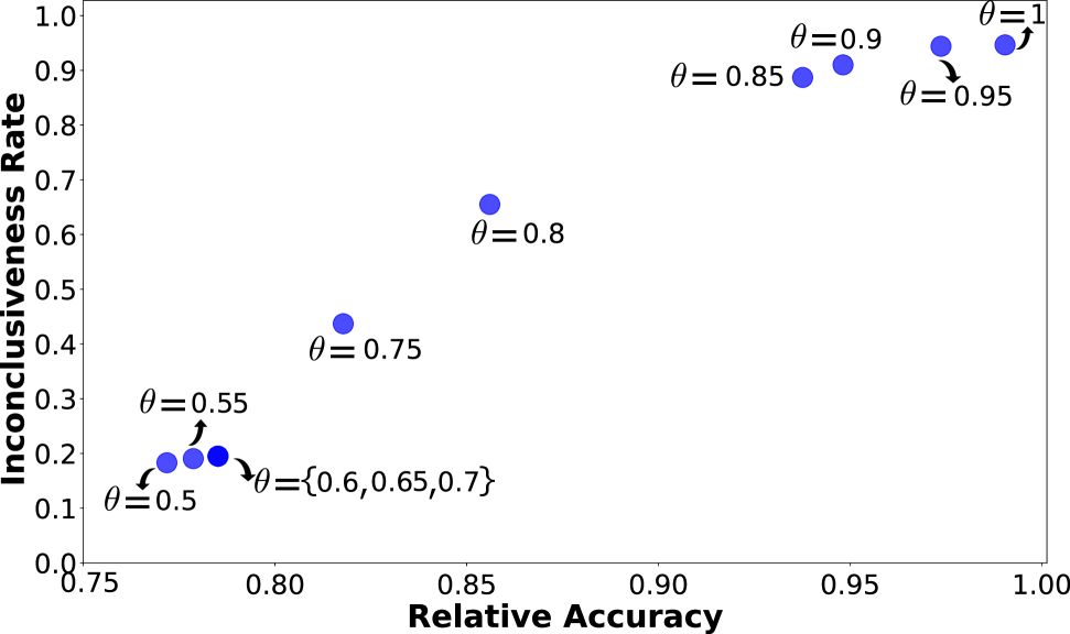
Figure 16: Trade-off between relative accuracy and inconclusiveness rate of test oracles generated by $\mathit{GP_{O}}$ for the router case study

For systems where minimizing the likelihood of mistakenly predicting a fail verdict as a pass is critical, we recommend setting $\theta$ to a high value (e.g., $\theta\geq 0.9$). At this threshold, pass/fail predictions are highly accurate, with zero or negligible (<3%) instances of this error. However, higher verdict thresholds (e.g., $\theta\geq 0.9$) typically increase the inconclusiveness rate, resulting in fewer tests receiving a conclusive verdict. In CPS simulators, where each test execution takes several minutes and multiple executions of the same test input are needed due to flakiness, high verdict thresholds can still yield substantial time savings. For instance, with $\theta\geq 0.9$, test oracles generated by GenTC for the AP–TWN(R3) case study produce conclusive predictions for 24% of tests, with 100% relative accuracy. Given the high flakiness rate and time-consuming nature of ADS simulations (each taking at least three minutes, as shown in Table I), skipping execution for 24% of tests represents significant time savings.

To determine optimal values for $\theta$, we calculate both inconclusiveness and relative accuracy using GenTC’s training set alone, eliminating the need for developing any additional set. As previously noted in this section, GenTC’s training sets are generated directly from the actual system’s executions, employing test generation techniques that diversify test inputs. This ensures that the training set represents the behaviour of the underlying SUT and can be used to identify the optimal $\theta$ values.

VII Related Work

This section compares our work with the relevant strands in five areas: (a) automating test oracles, (b) inferring assertions or grammars to explain system behaviours and their underlying causes, (c) SBFL ranking functions, (d) surrogate modelling, and (e) flaky tests.

VII-A Test Oracle Automation

To better position our work within the literature on test oracle generation, we present in Table VIII a structured comparison with the research strands most closely related to our work. We use the following criteria for the comparison:

TABLE VIII: Comparison of GenTC with related work strands on automating test oracles and inferring assertions to explain system behaviours

Approach(es)	Oracle Basis	Interpretability	Application Domain	Inference Method	Flakiness Studied?	Scope	Approach Access Level
[63, 64, 65]	Program variables (SUT execution needed)	✓	Generic-input Systems	Assertions generated by dynamic analysis	✗	Test Oracle Generation	White box
[66, 67, 68, 69, 70, 71]	System inputs and outputs (SUT execution needed)	✓	Generic-input Systems	Metamorphic relations designed manually or learned using GP	✗	Test Oracle Generation	White box
[13, 12, 72, 73, 74, 75, 76, 77, 9, 10, 11, 8, 78, 79]	System inputs and outputs (SUT execution needed)	✗	Generic-input Systems	Test oracles are Adaptive boosting, Neural networks	✗	Test Oracle Generation	Black box
[80, 81, 82]	System inputs and outputs (SUT execution needed)	✓	Numeric-input Systems	Metamorphic relations designed manually or learned using GP or partical swarm optimization	✗	Test Oracle Generation	Black box
[13, 12, 72, 73, 74, 75, 76, 77, 9, 10, 11, 8, 78, 79]	System inputs and outputs (SUT execution needed)	✗	Generic-input Systems	Test oracles are Adaptive boosting, Neural networks	✗	Test Oracle Generation	Black box
[14]	System inputs (SUT execution not needed)	✓	Numeric-input Systems	Test oracles are Incremental SMT Constraint Learner (INCAL), DT, Adaptive boosting, Support vector machine, Naïve bayes, Neural networks	✗	Automatic Program Repair, Test Oracle Generation	Black box
[83]	System inputs (SUT execution not needed)	✓	String-input Systems	Grammars inferred by input-abstraction methods	✗	Test Oracle Generation	Black box
[84]	System inputs (SUT execution not needed)	✓	String-input Systems	Grammars inferred by input-abstraction methods	✗	Learning Circumstances of System Behaviour	Black box
[85]	System inputs (SUT execution not needed)	✓	String-input Systems	Probabilistic grammars inferred by statistical methods	✗	Test Generation	Black box
[86]	System inputs (SUT execution not needed)	✓	String-input Systems	Test oracle is DT	✗	Learning Circumstances of System Behaviour	Black box
[30, 43, 31]	System inputs (SUT execution not needed)	✓	Numeric-input Systems	Assertions generated by DT, DR or GP	✗	Learning Circumstances of System Behaviour	Black box
[87, 88, 89]	System outputs (SUT execution needed)	✓	Generic-input Systems	Approximate assertions developed manually or by statistical methods	✓	Test Oracle Generation	Black box
GenTC	System inputs (SUT execution not needed)	✓	Numeric-input Systems	Assertions generated by GP	✓	Test Oracle Generation	Black box

¹ Manually designed metamorphic relations do not require executing the SUT, making the study of flakiness irrelevant to these approaches.
² Test oracles generated by adaptive boosting, support vector machine, naïve bayes and neural networks are not interpretable.
³ Inference method requires an input grammar of SUT.

(1) Oracle basis refers to the elements used to define test oracles. Oracle bases typically include program-specific elements – such as variables and function returns – as well as system-level inputs and outputs. For example, dynamic analysis techniques such as Daikon [63] build test oracles as program invariants defined based on program variables, while black-box approaches such as GAssertMRs [80] typically infer test oracles defined based on system-level inputs and/or outputs. When test oracles rely only on test inputs, they predict verdicts without requiring the execution of the SUT. In contrast, test oracles that depend on both inputs and outputs necessitate system execution.

(2) Interpretability refers to the test oracle’s ability to provide an understandable explanation of the reasoning behind the verdict it predicts. Typically, test oracles based on assertions, interpretable ML models, formal grammars and metamorphic relations are considered interpretable because their decision-making processes can be traced and explained through explicit rules. In contrast, non-interpretable test oracles are those based on non-interpretable ML models, such as neural networks or support vector machines.

(3) Application domain denotes the specific types of SUTs an approach targets. As shown in Table VIII, some approaches are designed for generic-input systems with no assumptions about input types. In contrast, others are tailored specifically to systems with string inputs [83, 84] or numeric inputs [30, 31, 14].

(4) Inference method refers to the approach used to generate test oracles. For string-input systems, test oracles may be inferred as context-free grammars that can distinguish syntactically valid and invalid test inputs for the SUT. Test oracles for generic-input and numeric-input systems are typically captured using metamorphic relations or ML models such as neural networks, Naïve Bayes, DT, or DR. Metamorphic relations may either be manually designed or automatically generated using heuristic techniques such as GP or particle swarm optimization.

(5) Flakiness studied indicates whether the approach considers potential flakiness in the SUT and examines its impact on the generated test oracles. Most approaches listed in Table VIII require executing the underlying SUT, making potential flakiness a relevant consideration for them.

(6) Scope indicates the primary objective of the proposed approach in the study. As shown in Table VIII, some approaches focus on test oracle generation, while others aim to learn or explain the circumstances underlying SUT behaviour. In some cases, the goal is to generate a test suite for program repair.

(7) Approach access-level refers to the level of access required by the inference method. Access-level can be categorized as either white box or black box. A white-box approach requires access to the SUT’s source code for instrumentation, while a black-box approach operates without needing insight into the SUT’s code.

Having set the stage with Table VIII, we now discuss the specific work strands listed in the table. We begin with an overview of test oracle automation techniques, followed by an outline of techniques aimed at explaining the circumstances behind SUT behaviour.

Automating test oracles. Recent research aims to reduce the oracle cost problem by developing automated test oracles that generate verdicts without human intervention or system execution [90]. Dynamic analysis techniques have been proposed to infer such oracles [64, 91, 65]. For example, Ernst et al. [63] introduced Daikon, a dynamic analysis tool that observes program behaviour by running the software with various inputs and capturing values at different points in the code. These values are analyzed to infer potential invariants, such as variable relationships and properties that hold across executions. This approach requires direct access to the program’s code for instrumentation, which restricts its use in heterogeneous CPS that may include proprietary or closed subsystems where effective instrumentation is not feasible.

Several studies use metamorphic testing to detect system failures by identifying violations of metamorphic relations (MRs) [66, 67, 68, 69, 70, 71, 81]. MRs predict expected outputs for different test inputs, and hence, can be used as test oracles [92]. Identifying MRs is primarily a manual, time-consuming task that requires domain expertise [93]. Automated identification methods for MRs often rely on access to the source code [67, 68, 69], datasets of test inputs and outputs [82, 80, 71], or existing MRs of the SUT [66, 68]. Our work is closely related to studies that learn MRs from test inputs and outputs; however, we focus on learning assertions instead. Unlike these studies, our work explicitly investigates the impact of flakiness on the learned assertions.

Recent research has focused on adopting a data-driven approach to test oracle automation, where test oracles are developed using ML models such as Adaptive Boosting [13, 14] or Neural Networks [12, 14, 72, 73, 74, 75, 76, 77, 78, 79]. However, these ML models lack interpretability, which is crucial for CPS systems. An exception is the learn2fix framework [14] that develops test oracles using two interpretable models, DT and the Incremental SMT Constraint Learner (INCAL) [94]. We show that assertion-based test oracles generated using GP are significantly more accurate than those generated using DT. While assertion-based test oracles can theoretically be derived using INCAL, we excluded INCAL from our evaluation due to its scalability limitations. When applied to our case studies, INCAL failed to generate assertion-based test oracles even after providing it with a large time budget of several hours.

Inferring assertions or grammars to explain behaviours of SUT and their underlying causes. Several studies have explored inferring assertions or grammars that explain particular behaviours of a SUT [83, 84, 85, 86, 30, 31, 43]. For instance, approaches that aim to explain the circumstances of failure typically start with one or more known examples. They then generate additional tests iteratively, and infer assertions or grammars that explain the underlying causes of these failures. Such assertions can serve as test oracles and be used to predict test verdicts [83, 86, 30, 43]. Several other studies have developed approximate assertions for ML frameworks and probabilistic programming systems [87, 88, 89]. Approximate assertions determine test verdicts by comparing the SUT’s outputs against expected ranges defined by statistical bounds or probabilistic thresholds. Rather than requiring exact output matches, the assertions check whether the observed outputs fall within these predefined acceptable bounds. Because these assertions rely on output evaluation, they require executing the SUT to collect output data for comparison. These studies mainly focus on detecting and fixing flaky tests by adjusting the thresholds that define acceptable output deviations for assertions [88, 89].

In contrast to existing assertion-inferring approaches, our work is the first to define assertion-based test oracles over the inputs of the SUT specifically for CPS. We propose a novel approach that employs interpretable techniques to generate assertion-based test oracles. Our evaluation focuses on flaky CPS simulators where we examine the impact of flakiness on the accuracy of the generated oracles for these systems.

VII-B SBFL Ranking Functions

Several studies use SBFL ranking functions to pinpoint faulty program statements [95]. There are more than $30$ ranking functions studied in the SBFL literature [96, 17]. Among these, Tarantula, Ochiai and Naish have been studied more extensively compared to other ranking functions. Tarantula [16] is among the first ranking functions proposed for SBFL. Ochiai was originally used in molecular biology for measuring genetic similarity and was later adopted by SBFL for fault localization [15]. Naish has been introduced more recently and has shown competitive performance compared to Ochiai in some studies [17, 97]. These functions have proven effective in correlating program statements (i.e., assertions in our work) with the pass and fail verdicts of a test suite.

Most SBFL ranking functions are designed manually [98]. GP has been employed to automatically generate SBFL ranking functions [98]. The ranking functions generated by GP are usually complex and involve various mathematical operators. This risks overfitting to specific SUT behaviours that only appear in the training sets. Consequently, using the GP-learned ranking functions to derive assertion-based test oracles may lead to test oracles that fail to generalize. In our work, we show that test oracles generated using Ochiai are more accurate than those generated using Tarantula or Naish, as well as those generated by DT and DR. Further, we are the first to explore the effectiveness of SBFL ranking functions as fitness functions of GP for generating accurate and robust test oracles for CPS. SBFL ranking functions are particularly suitable as GP fitness functions for assertion generation, as they provide a smooth fitness landscape – an essential property for the effectiveness of GP [29]. In contrast, fitness functions such as the one used by Gaaloul et al. [31] strictly prioritize soundness of candidate assertions, rewarding coverage only when no pass (resp. fail) tests satisfy a fail (resp. pass) candidate assertion. While this helps reduce incorrect predictions by assertions, it results in a non-smooth fitness landscape – small changes to a candidate assertion can cause abrupt shifts in fitness. As a result, fail (resp. pass) assertions that correctly capture a large portion of fail (resp. pass) tests but include a small number of pass (resp. fail) tests are penalized heavily and prematurely discarded. Heuristic search is less effective for fitness functions with a non-smooth landscape [29].

VII-C Surrogate Modelling

Recent research suggests using surrogate models to bypass system executions by creating models that approximate complex mathematical systems [30, 99, 100]. These surrogate models predict system outputs or test verdicts based on test inputs without running the actual system. Most existing surrogate models rely on non-interpretable ML techniques such as neural networks [101, 102], or on regression approaches such as polynomial regression [103, 99]. Because we consider interpretability essential, we focus only on models that can generate human-readable assertions. We note that decision trees and decision rules have been used in the literature as surrogate models [30, 104, 105]; to our knowledge, they are the only surrogate-modelling techniques capable of producing interpretable assertions. These models are included in our evaluation, and we have compared them with GP techniques in terms of both accuracy and robustness. Our results in RQ2 and RQ3 show that GP with Ochiai generates more accurate and robust test oracles than decision trees or decision rules.

VII-D Flaky Tests

Recent studies show that flaky tests are prevalent in both commercial and open-source software projects. For example, Google reported that nearly $16\%$ of their $4.2$ million test cases are flaky [106], and the Microsoft Windows and Dynamics teams estimated a $5\%$ rate of flaky test failures [107]. Prior research has explored the root causes of flaky tests and proposed techniques for addressing them across a range of systems, including open-source software [5], embedded systems [108], probabilistic programming systems [88], and ML frameworks [88, 89]. Common sources of flakiness include asynchronous waits, concurrency, test-order dependencies, and non-determinism in algorithmic behaviour. As shown in RQ1 (Section V), our study subjects – drawn from aerospace, networking, and autonomous driving domains – show varying levels of flakiness, often due to environmental variability, unpredictable hardware-software interactions, and underlying stochastic processes.

Several techniques have been developed to detect flaky tests, such as analyzing test execution order [109], identifying data dependencies among tests [110], and rerunning tests under different random seeds [88]. Our work differs from this line of research: rather than detecting or fixing flaky tests, we focus on evaluating the robustness of test oracles learned from training sets that include flaky tests. Our robustness analysis helps determine whether flaky tests should be excluded from training sets or retained, depending on whether their inclusion significantly impacts the accuracy of the test oracles. Our findings from RQ3 indicate that, when using GP with Ochiai, the average variation in prediction accuracy is around 4%. If this variation is acceptable, flaky tests can remain in training sets, thereby reducing costs associated with detecting and removing them.

VIII Conclusion

In this article, we introduced assertion-based test oracles and evaluated them for accuracy and robustness. These oracles reduce dependence on simulator executions by enabling the prediction of pass and fail verdicts directly from test inputs. Our approach to building test oracles ensures that they issue consistent verdicts and provide human-understandable explanations of those verdicts. We constructed test oracles using genetic programming (GP) and machine learning (ML), leveraging spectrum-based fault localization formulas – Tarantula, Ochiai, and Naish – as fitness functions to evolve accurate and effective assertions. Our formal analysis demonstrated that assertion-based test oracles possess sufficient expressive power to capture a wide range of CPS properties, and our empirical evaluation across diverse domains showed that they deliver accurate and robust predictions even under conditions of test flakiness. Specifically, based on empirical results from five aerospace, autonomous driving, and networked systems, we showed that test oracles generated by GP using Ochiai achieve high accuracy and robustness, even when inferred from training sets that include flaky tests. In particular, test oracles generated by GP with Ochiai were robust to flakiness, with only a $4$% variation in accuracy. Our full replication package is available online [27].

Appendix A Equivalence between logic fragment $\mathcal{L}$ and grammar $\mathcal{G}$

We show equivalence by constructing bidirectional transformations between any formula in $\mathcal{L}$ and conditions expressed by the grammar $\mathcal{G}$ defined in Figure 5.

(1) Transforming a formula in $\mathcal{L}$ to a condition based on grammar $\mathcal{G}$. We show that any formula $\phi$ written in $\mathcal{L}$ can be expressed as a condition based on our grammar $\mathcal{G}$.

Proof.

We proceed by structural induction on the structure of $\phi\in\mathcal{L}$.

Base Cases.

• Base Case 1: $\mathbf{\phi=r\sim 0}$
  Let $\phi=r\sim 0$ where $\sim\in\{<,\leq,>,\geq,=,\neq\}$. Based on the definition of $\mathcal{L}$ in Section IV-C, we have $r\in\mathbb{R}$. Therefore, $r$ maps to const in grammar $\mathcal{G}$. Thus, $r\sim 0$ corresponds to const $\sim$ 0, which is a rel-term in grammar $\mathcal{G}$.

• Base Case 2: $\mathbf{\phi=\forall t\in\langle n_{1},n_{2}\rangle:u(t)\sim 0}$
  Let $\phi=\forall t\in\langle n_{1},n_{2}\rangle:u(t)\sim 0$, where $u$ is a signal over the time domain $\mathbb{T}=[0,b]$, and $\langle n_{1},n_{2}\rangle$ is a subinterval of $\mathbb{T}$. Based on Section IV-B, $u$ is encoded using $n_{u}$ control points, i.e., $c_{u,0},\ldots,c_{u,n_{u}-1}$ each placed at time instants $0,I,2\cdot I,\ldots,(n_{u}-1)\cdot I$, where $I=\frac{b}{n_{u}-1}$. Under the piecewise constant interpolation assumption, the value of $u(t)$ is constant within each interval $[j\cdot I,(j+1)\cdot I)$ and equal to $c_{u,j}$.

  If the interval $\langle n_{1},n_{2}\rangle$ is contained within a single time interval $[j\cdot I,(j+1)\cdot I)$, then $\forall t\in\langle n_{1},n_{2}\rangle:u(t)$ maps to $c_{u,j}$ which is control point cp in grammar $\mathcal{G}$. Thus, $\forall t\in\langle n_{1},n_{2}\rangle:u(t)\sim 0$ corresponds to cp $\sim 0$ which is a rel-term in grammar $\mathcal{G}$.

  If $\langle n_{1},n_{2}\rangle$ spans multiple control-point intervals (e.g., $[j\cdot I,(j+k)\cdot I)$ for some $k\geq 2$), then $\forall t\in\langle n_{1},n_{2}\rangle:u(t)\sim 0$ can be decomposed into conjunctions over each unit interval:

  $\forall t\in[j\cdot I,(j+1)\cdot I):u(t)\sim 0\ \land\ldots\land\forall t\in[(j+k-1)\cdot I,(j+k)\cdot I):u(t)\sim 0$.

  Each subformula $\forall t\in[i\cdot I,(i+1)\cdot I):u(t)\sim 0$ is semantically equivalent to $c_{u,i}\sim 0$. Hence, the entire formula corresponds to:

  $c_{u,j}\sim 0\ \land c_{u,j+1}\sim 0\ \land\ldots\land c_{u,j+k-1}\sim 0$

  which is an and-term over rel-terms in grammar $\mathcal{G}$.

• Base Case 3: $\mathbf{\phi=\forall t\in\langle n_{1},n_{2}\rangle:\rho\sim 0}$
  Based on the definition of $\mathcal{L}$ in Section IV-C, $\rho::=u(t)\mid r\mid\rho_{1}+\rho_{2}\mid\rho_{1}-\rho_{2}\mid\rho_{1}\times\rho_{2}\mid\rho_{1}/\rho_{2}$. By the inductive structure of $\rho$, $\rho_{1}$ and $\rho_{2}$ are each either $u(t)$ or a constant $r$, or further composed of arithmetic terms. We note that based on Section IV-C, $\mathcal{L}$ does not allow nested quantifiers, hence, no additional quantifiers (i.e., $\forall t$) appear in $\phi$.

  As in Base Cases 1 and 2, each occurrence of $u(t)$ within the interval $\langle n_{1},n_{2}\rangle$ can be replaced with the corresponding control point $c_{u,j}$. Further, each occurrence of $r$ remains as is. Therefore, $\rho_{1}$ and $\rho_{2}$ can be rewritten into arithmetic expressions over control points and constants, i.e., valid exps in $\mathcal{G}$. Hence, the formula $\forall t\in\langle n_{1},n_{2}\rangle:\rho\sim 0$ corresponds to an expression like exp $\sim 0$ over control points and constants, which is a rel-term in grammar $\mathcal{G}$.

Inductive Cases.

• Inductive Case 1: $\mathbf{\phi=\phi_{1}\wedge\phi_{2}}$
  The inductive hypothesis is that $\phi_{1}$ and $\phi_{2}$ correspond to rel-terms or and-terms in grammar $\mathcal{G}$. Since we assume that no free time variables exist in $\phi_{1}$ and $\phi_{2}$ based on Section IV-C, $\phi_{1}$ and $\phi_{2}$ ultimately reduce to one of the base cases—either a simple relational expression over constants (Base Case 1), over control points (Base Case 2) or over arithmetic expressions (Base Case 3). Hence, $\phi_{1}\wedge\phi_{2}$ is a conjunction of expressions derived from base cases and hence corresponds to an and-term in grammar $\mathcal{G}$.

• Inductive Case 2: $\mathbf{\phi=\phi_{1}\vee\phi_{2}}$
  Similar to Inductive Case 1, by the inductive hypothesis, both $\phi_{1}$ and $\phi_{2}$ correspond to rel-terms or and-terms in grammar $\mathcal{G}$. As there are no free time variables, all expressions in $\phi_{1}$ and $\phi_{2}$ are grounded in the base cases, making them structurally reducible to rel-terms or and-terms. Hence, $\phi_{1}\vee\phi_{2}$ is a disjunction of expressions derived from base cases and hence corresponds to an or-term in grammar $\mathcal{G}$.

Therefore, every formula $\phi\in\mathcal{L}$ corresponds to a well-formed condition in grammar $\mathcal{G}$. ∎

(2) Transforming a condition in $\mathcal{G}$ to a formula in $\mathcal{L}$. The transformation of any condition in $\mathcal{G}$ into a formula in $\mathcal{L}$ can be established analogously, using structural induction on the grammar $\mathcal{G}$. Briefly,

• Each control point cp corresponds to a sub-interval of the time domain where the signal $u(t)$ is constant; thus, each control point maps to a formula $\forall t\in\langle n_{1},n_{2}\rangle:u(t)$ in $\mathcal{L}$ by the piecewise constant assumption. Further, each const corresponds to $r$ in logic $\mathcal{L}$.

• Each rel-term corresponds directly to a formula of the form $\rho\sim 0$ in $\mathcal{L}$, where $\rho$ is an arithmetic expression over signals and constants.

• Each and-term corresponds to conjunction $\phi_{1}\wedge\phi_{2}$, and each or-term corresponds to disjunction $\psi_{1}\vee\psi_{2}$ in $\mathcal{L}$.

Hence, the transformation from grammar $\mathcal{G}$ to logic $\mathcal{L}$ follows the same structural induction as in (1) and is omitted for brevity.

Conclusion. Based on (1) and (2), we have equivalence between logic fragment $\mathcal{L}$ and grammar $\mathcal{G}$, meaning that for every formula in $\mathcal{L}$ there exists a condition in $\mathcal{G}$, and for every condition in $\mathcal{G}$ there exists a formula in $\mathcal{L}$, with both transformations preserving the original semantics.

Appendix B Supplementary results for RQ2 and RQ3

This section presents the statistical-test results for RQ2 and RQ3. Detailed discussions of these tables are provided in Sections V-C and  V-D.

TABLE IX: Statistical tests comparing the accuracy results of $\mathit{GP_{O}}$ against those of $\mathit{GP_{T}}$, $\mathit{GP_{N}}$, DT, DR and ensemble. The p-values highlighted in blue represent cases where $\mathit{GP_{O}}$ significantly outperforms the compared alternative. The significance level is $0.05$.

	$\mathit{GP_{O}}$ vs $\mathit{GP_{T}}$		$\mathit{GP_{O}}$ vs $\mathit{GP_{N}}$		$\mathit{GP_{O}}$ vs DT		$\mathit{GP_{O}}$ vs DR		$\mathit{GP_{O}}$ vs Ensemble
$\theta$	P-value	$\mathbf{\hat{A}_{12}}$	P-value	$\mathbf{\hat{A}_{12}}$	P-value	$\mathbf{\hat{A}_{12}}$	P-value	$\mathbf{\hat{A}_{12}}$	P-value	$\mathbf{\hat{A}_{12}}$
0.5	1.05E-25 $GP_{O}>GP_{T}$	0.86 (L)	0.03 $GP_{O}>GP_{N}$	0.57 (S)	1.59E-25 $GP_{O}>DT$	0.85 (L)	4.3E-45 $GP_{O}>DR$	0.98 (L)	7.83E-21 $GP_{O}>Ensemble$	0.82 (L)
0.55	3.59E-26 $GP_{O}>GP_{T}$	0.87 (L)	0.01 $GP_{O}>GP_{N}$	0.59 (S)	2.14E-25 $GP_{O}>DT$	0.85 (L)	2.56E-44 $GP_{O}>DR$	0.97 (L)	1.98E-19 $GP_{O}>Ensemble$	0.81 (L)
0.6	1.5E-21 $GP_{O}>GP_{T}$	0.84 (L)	0.04 $GP_{O}>GP_{N}$	0.57 (S)	3.33E-22 $GP_{O}>DT$	0.84 (L)	5.07E-41 $GP_{N}>DR$	0.98 (L)	7E-16 $GP_{O}>Ensemble$	0.79 (L)
0.65	9.03E-23 $GP_{O}>GP_{T}$	0.88 (L)	5.55E-08 $GP_{O}>GP_{N}$	0.71 (L)	7.74E-18 $GP_{O}>DT$	0.83 (L)	3.68E-36 $GP_{O}>DR$	0.98 (L)	9.48E-18 $GP_{O}>Ensemble$	0.83 (L)
0.7	1.19E-24 $GP_{O}>GP_{T}$	0.92 (L)	1.51E-07 $GP_{O}>GP_{N}$	0.73 (L)	3.37E-16 $GP_{O}>DT$	0.84 (L)	8.42E-32 $GP_{O}>DR$	0.98 (L)	1.6E-20 $GP_{O}>Ensemble$	0.88 (L)
0.75	1.24E-19 $GP_{O}>GP_{T}$	0.94 (L)	4.42E-11 $GP_{O}>GP_{N}$	0.85 (L)	1.09E-14 $GP_{O}>DT$	0.87 (L)	1.14E-22 $GP_{O}>DR$	0.97 (L)	1.51E-17 $GP_{O}>Ensemble$	0.91 (L)
0.8	2.9E-14 $GP_{O}>GP_{T}$	0.94 (L)	6.45E-06 $GP_{O}>GP_{N}$	0.78 (L)	3.33E-08 $GP_{O}>DT$	0.81 (L)	6.42E-17 $GP_{O}>DR$	0.97 (L)	2.33E-11 $GP_{O}>Ensemble$	0.88 (L)
0.85	3.61E-13 $GP_{O}>GP_{T}$	0.96 (L)	0.004 $GP_{O}>GP_{N}$	0.72 (L)	3.15E-08 $GP_{O}>DT$	0.84 (L)	2.47E-14 $GP_{O}>DR$	0.97 (L)	3.3E-10 $GP_{O}>Ensemble$	0.89 (L)
0.9	0.0004 $GP_{O}>GP_{T}$	0.85 (L)	0.97 $GP_{O}\approx GP_{N}$	0.50 (N)	0.81 $GP_{O}\approx DT$	0.52 (N)	0.0003 $GP_{O}>DR$	0.85 (L)	0.12 $GP_{O}\approx Ensemble$	0.65 (M)
0.95	0.001 $GP_{O}>GP_{T}$	0.89 (L)	0.67 $GP_{O}\approx GP_{N}$	0.57 (S)	0.84 $GP_{O}\approx DT$	0.47 (N)	0.0002 $GP_{O}>DR$	0.93 (L)	0.16 $GP_{O}\approx Ensemble$	0.66 (M)
1	0.001 $GP_{O}>GP_{T}$	0.91 (L)	0.74 $GP_{O}\approx GP_{N}$	0.57 (S)	0.28 $GP_{O}\approx DT$	0.36 (M)	0.001 $GP_{O}>DR$	0.91 (L)	0.18 $GP_{O}\approx Ensemble$	0.67 (M)

TABLE X: Statistical tests comparing the accuracy results of $\mathit{GP_{O}}$ against those of $\mathit{GP_{T}}$, $\mathit{GP_{N}}$, DT, DR and ensemble for each study subject. The p-values highlighted in blue represent cases where $\mathit{GP_{O}}$ significantly outperforms the compared alternative. The p-values highlighted in orange indicate cases where the compared alternative outperforms $\mathit{GP_{O}}$. The cells highlighted in yellow represent cases where DT is not applicable. The significance level is $0.05$.

	$\mathit{GP_{O}}$ vs $\mathit{GP_{T}}$		$\mathit{GP_{O}}$ vs $\mathit{GP_{N}}$		$\mathit{GP_{O}}$ vs DT		$\mathit{GP_{O}}$ vs DR		$\mathit{GP_{O}}$ vs Ensemble
Study Subject	P-value	$\mathbf{\hat{A}_{12}}$	P-value	$\mathbf{\hat{A}_{12}}$	P-value	$\mathbf{\hat{A}_{12}}$	P-value	$\mathbf{\hat{A}_{12}}$	P-value	$\mathbf{\hat{A}_{12}}$
Router	1.9E-33 $GP_{O}>GP_{T}$	0.87 (L)	8.4E-05 $GP_{O}>GP_{N}$	0.62 (S)	4.55E-15 $DT>GP_{O}$	0.29 (L)	4.72E-51 $GP_{O}>DR$	0.91 (L)	6.58E-07 $GP_{O}>Ensemble$	0.65 (M)
AP–DHB	0.0001 $GP_{O}>GP_{T}$	0.68 (L)	0.16 $GP_{N}\approx GP_{O}$	0.43 (S)	1.64E-59 $GP_{O}>DT$	1 (L)	2.75E-26 $GP_{O}>DR$	1 (L)	1.93E-09 $GP_{O}>Ensemble$	0.77 (L)
AP–TWN (R1)	1.37E-11 $GP_{O}>GP_{T}$	1 (L)	6.69E-11 $GP_{O}>GP_{N}$	1 (L)	9.01E-12 $GP_{O}>DT$	1 (L)	4.42E-13 $GP_{O}>DR$	1 (L)	2.06E-11 $GP_{O}>Ensemble$	1 (L)
AP–TWN (R2)	0.002 $GP_{O}>GP_{T}$	0.60 (S)	0.17 $GP_{N}\approx GP_{O}$	0.54 (N)	1.83E-12 $GP_{O}>DT$	0.72 (L)	7.52E-66 $GP_{O}>DR$	1 (L)	0.01 $Ensemble>GP_{O}$	0.41 (S)
AP–TWN (R3)	9.1E-33 $GP_{O}>GP_{T}$	1 (L)	1.01E-22 $GP_{O}>GP_{N}$	0.91 (L)	3.66E-69 $GP_{O}>DT$	1 (L)	4.72E-51 $GP_{O}>DR$	1 (L)	3.48E-43 $GP_{O}>Ensemble$	1 (L)
AP–TWN (R4)	1.41E-33 $GP_{O}>GP_{T}$	1 (L)	2.03E-15 $GP_{O}>GP_{N}$	0.82 (L)	DT is not applicable		6.13E-21 $GP_{O}>DR$	1 (L)	8.76E-33 $GP_{O}>Ensemble$	1 (L)
AP–SNG	8.5E-46 $GP_{O}>GP_{T}$	1 (L)	2.48E-42 $GP_{O}>GP_{N}$	1 (L)	7.42E-68 $GP_{O}>DT$	1 (L)	1.17E-50 $GP_{O}>DR$	1 (L)	1.83E-58 $GP_{O}>Ensemble$	1 (L)
Dave2	7.11E-13 $GP_{O}>GP_{T}$	0.78 (L)	0.02 $GP_{N}>GP_{O}$	0.40 (S)	1.24E-46 $GP_{O}>DT$	1 (L)	1.23E-22 $GP_{O}>DR$	0.86 (L)	6.78E-09 $GP_{O}>Ensemble$	0.72 (L)

TABLE XI: Statistical test results comparing (a) the rate of pass verdicts predicted as fail achieved with DR against those of $\mathit{GP_{T}}$, $\mathit{GP_{O}}$, $\mathit{GP_{N}}$, DT and ensemble (b) the rate of fail verdicts predicted as pass achieved with $\mathit{GP_{O}}$ against those of $\mathit{GP_{T}}$, $\mathit{GP_{N}}$, DT, DR and ensemble. The p-values highlighted in blue represent cases where the method on the left significantly outperforms the compared alternative. The p-values highlighted in orange indicate cases where the compared alternative significantly outperforms the method on the left. The significance level is $0.05$.

(a) Rate of pass verdicts predicted as fail

	DR vs $\mathit{GP_{T}}$		DR vs $\mathit{GP_{O}}$		DR vs $\mathit{GP_{N}}$		DR vs DT		DR vs Ensemble
$\theta$	P-value	$\mathbf{\hat{A}_{12}}$	P-value	$\mathbf{\hat{A}_{12}}$	P-value	$\mathbf{\hat{A}_{12}}$	P-value	$\mathbf{\hat{A}_{12}}$	P-value	$\mathbf{\hat{A}_{12}}$
0.5	2.85E-11 $DR>GP_{T}$	0.29 (L)	3.56E-15 $DR>GP_{O}$	0.24 (L)	6.28E-18 $DR>GP_{N}$	0.22 (L)	1.11E-10 $DR>DT$	0.30 (M)	1.32E-12 $DR>Ensemble$	0.28 (L)
0.55	3.72E-11 $DR>GP_{T}$	0.29 (L)	5.52E-15 $DR>GP_{O}$	0.24 (L)	3.83E-17 $DR>GP_{N}$	0.22 (L)	3E-10 $DR>DT$	0.30 (M)	1.1E-12 $DR>Ensemble$	0.28 (L)
0.6	9.75E-11 $DR>GP_{T}$	0.30 (M)	3.78E-14 $DR>GP_{O}$	0.24 (L)	3.83E-17 $DR>GP_{N}$	0.22 (L)	3E-10 $DR>DT$	0.30 (M)	1.09E-12 $DR>Ensemble$	0.28 (L)
0.65	3.24E-10 $DR>GP_{T}$	0.30 (M)	2.2E-13 $DR>GP_{O}$	0.23 (L)	2.31E-08 $DR>GP_{N}$	0.31 (M)	5.28E-06 $DR>DT$	0.35 (M)	2.09E-07 $DR>Ensemble$	0.34 (M)
0.7	3.94E-08 $DR>GP_{T}$	0.32 (M)	5.93E-22 $DR>GP_{O}$	0.11 (L)	3.68E-20 $DR>GP_{N}$	0.16 (L)	5.01E-06 $DR>DT$	0.35 (M)	1.83E-07 $DR>Ensemble$	0.34 (M)
0.75	1.88E-05 $DR>GP_{T}$	0.36 (M)	2.76E-12 $DR>GP_{O}$	0.17 (L)	2.52E-15 $DR>GP_{N}$	0.19 (L)	1.99E-05 $DR>DT$	0.36 (M)	0.0007 $DR>Ensemble$	0.39 (S)
0.8	0.0001 $DR>GP_{T}$	0.37 (S)	1.64E-13 $DR>GP_{O}$	0.10 (L)	3.82E-13 $DR>GP_{N}$	0.20 (L)	1.9E-05 $DR>DT$	0.36 (M)	6.5E-05 $DR>Ensemble$	0.37 (S)
0.85	0.0003 $DR>GP_{T}$	0.37 (S)	9.42E-14 $DR>GP_{O}$	0.06 (L)	3.19E-15 $DR>GP_{N}$	0.05 (L)	1.23E-05 $DR>DT$	0.35 (M)	7.44E-05 $DR>Ensemble$	0.37 (S)
0.9	4.3E-05 $DR>GP_{T}$	0.35 (M)	0.002 $DR>GP_{O}$	0.23 (L)	8.94E-07 $DR>GP_{N}$	0.11 (L)	3.26E-06 $DR>DT$	0.34 (M)	5.12E-05 $DR>Ensemble$	0.36 (M)
0.95	0.0006 $DR>GP_{T}$	0.37 (S)	0.01 $DR>GP_{O}$	0.23 (L)	6.06E-06 $DR>GP_{N}$	0.07 (L)	0.0003 $DR>DT$	0.37 (S)	0.003 $DR>Ensemble$	0.39 (S)
1	2.82E-05 $DR>GP_{T}$	0.33 (M)	0.03 $DR>GP_{O}$	0.26 (L)	3.69E-05 $DR>GP_{N}$	0.09 (L)	2.13E-05 $DR>DT$	0.33 (M)	0.001 $DR>Ensemble$	0.38 (S)

(b) Rate of fail verdicts predicted as pass

	$\mathit{GP_{O}}$ vs $\mathit{GP_{T}}$		$\mathit{GP_{O}}$ vs $\mathit{GP_{N}}$		$\mathit{GP_{O}}$ vs DT		$\mathit{GP_{O}}$ vs DR		$\mathit{GP_{O}}$ vs Ensemble
$\theta$	P-value	$\mathbf{\hat{A}_{12}}$	P-value	$\mathbf{\hat{A}_{12}}$	P-value	$\mathbf{\hat{A}_{12}}$	P-value	$\mathbf{\hat{A}_{12}}$	P-value	$\mathbf{\hat{A}_{12}}$
0.5	0.03 $GP_{O}>GP_{T}$	0.43 (S)	0.07 $GP_{O}\approx GP_{N}$	0.43 (S)	0.02 $GP_{O}>DT$	0.42 (S)	0.0006 $GP_{O}>DR$	0.38 (S)	0.08 $GP_{O}\approx Ensemble$	0.44 (N)
0.55	0.61 $GP_{O}\approx GP_{T}$	0.48 (N)	0.06 $GP_{O}\approx GP_{N}$	0.43 (S)	0.72 $GP_{O}\approx DT$	0.51 (N)	0.20 $GP_{O}\approx DR$	0.45 (N)	0.88 $GP_{O}\approx Ensemble$	0.50 (N)
0.6	0.03 $GP_{O}>GP_{T}$	0.43 (S)	0.001 $GP_{O}>GP_{N}$	0.39 (S)	0.03 $GP_{O}>DT$	0.43 (S)	0.0001 $GP_{O}>DR$	0.36 (M)	0.06 $GP_{O}\approx Ensemble$	0.43 (S)
0.65	0.02 $GP_{O}>GP_{T}$	0.42 (S)	0.03 $GP_{O}\approx GP_{N}$	0.42 (S)	0.0005 $GP_{O}>DT$	0.37 (S)	0.0002 $GP_{O}>DR$	0.36 (M)	0.01 $GP_{O}>Ensemble$	0.41 (S)
0.7	3.47E-06 $GP_{O}>GP_{T}$	0.34 (M)	0.008 $GP_{O}>GP_{N}$	0.42 (S)	9.12E-15 $GP_{O}>DT$	0.19 (L)	1.91E-13 $GP_{O}>DR$	0.21 (L)	8.52E-10 $GP_{O}>Ensemble$	0.27 (L)
0.75	0.001 $GP_{O}>GP_{T}$	0.38 (S)	0.27 $GP_{O}\approx GP_{N}$	0.52 (N)	7.6E-11 $GP_{O}>DT$	0.19 (L)	7.67E-08 $GP_{O}>DR$	0.25 (L)	6.19E-07 $GP_{O}>Ensemble$	0.28 (L)
0.8	0.32 $GP_{O}\approx GP_{T}$	0.46 (N)	0.05 $GP_{O}\approx GP_{N}$	0.54 (N)	7.79E-07 $GP_{O}>DT$	0.22 (L)	0.19 $GP_{O}\approx DR$	0.44 (N)	0.0005 $GP_{O}>Ensemble$	0.32 (M)
0.85	0.89 $GP_{O}\approx GP_{T}$	0.50 (N)	0.63 $GP_{O}\approx GP_{N}$	0.52 (N)	8.38E-06 $GP_{O}>DT$	0.22 (L)	0.45 $GP_{O}\approx DR$	0.46 (N)	0.002 $GP_{O}>Ensemble$	0.32 (M)
0.9	0.002 $GP_{T}>GP_{O}$	0.64 (M)	0.50 $GP_{O}\approx GP_{N}$	0.56 (S)	0.80 $GP_{O}\approx DT$	0.47 (N)	0.18 $GP_{O}\approx DR$	0.59 (S)	0.56 $GP_{O}\approx Ensemble$	0.54 (N)
0.95	0.0003 $GP_{T}>GP_{O}$	0.65 (M)	0.44 $GP_{O}\approx GP_{N}$	0.59 (S)	0.83 $GP_{O}\approx DT$	0.52 (N)	0.39 $GP_{O}\approx DR$	0.57 (S)	0.26 $GP_{O}\approx Ensemble$	0.59 (S)
1	6.99E-05 $GP_{T}>GP_{O}$	0.68 (M)	0.52 $GP_{O}\approx GP_{N}$	0.60 (S)	0.88 $GP_{O}\approx DT$	0.52 (N)	0.34 $GP_{O}\approx DR$	0.60 (S)	0.24 $GP_{O}\approx Ensemble$	0.61 (S)

TABLE XII: Statistical test results comparing (a) the rate of pass verdicts predicted as fail achieved with DR against those of $\mathit{GP_{T}}$, $\mathit{GP_{O}}$, $\mathit{GP_{N}}$, DT and ensemble (b) the rate of fail verdicts predicted as pass achieved with $\mathit{GP_{O}}$ against those of $\mathit{GP_{T}}$, $\mathit{GP_{N}}$, DT, DR and ensemble for each study subject. The p-values highlighted in blue represent cases where the method on the left significantly outperforms the compared alternative. The p-values highlighted in orange indicate cases where the compared alternative significantly outperforms the method on the left. The cells highlighted in yellow represent cases where DT is not applicable. The significance level is $0.05$.

(a) Rate of pass verdicts predicted as fail

	DR vs $\mathit{GP_{T}}$		DR vs $\mathit{GP_{O}}$		DR vs $\mathit{GP_{N}}$		DR vs DT		DR vs Ensemble
Study Subject	P-value	$\mathbf{\hat{A}_{12}}$	P-value	$\mathbf{\hat{A}_{12}}$	P-value	$\mathbf{\hat{A}_{12}}$	P-value	$\mathbf{\hat{A}_{12}}$	P-value	$\mathbf{\hat{A}_{12}}$
Router	1.37E-49 $DR>GP_{T}$	0.13 (L)	4.95E-14 $DR>GP_{O}$	0.29 (L)	7.06E-17 $DR>GP_{N}$	0.27 (L)	1.18E-62 $DR>DT$	0.16 (L)	1.75E-58 $DR>Ensemble$	0.1 (L)
AP–DHB	2.34E-46 $DR>GP_{T}$	0.001 (L)	1.14E-24 $DR>GP_{O}$	0.01 (L)	5.19E-44 $DR>GP_{N}$	0 (L)	3.07E-67 $DR>DT$	0.03 (L)	8.41E-59 $DR>Ensemble$	0.01 (L)
AP–TWN (R1)	5.88E-38 $DR>GP_{T}$	0.19 (L)	1 $DR\approx GP_{O}$	0.5 (N)	6.48E-36 $DR>GP_{N}$	0.18 (L)	2.09E-59 $DR>DT$	0 (L)	9.9E-38 $DR>Ensemble$	0.19 (L)
AP–TWN (R2)	1 $DR\approx GP_{T}$	0.5 (N)	1.61E-21 $DR>GP_{O}$	0.31 (M)	2.35E-25 $DR>GP_{N}$	0.28 (L)	1 $DR\approx DT$	0.5 (N)	1 $DR\approx Ensemble$	0.5 (N)
AP–TWN (R3)	0.005 $DR>GP_{T}$	0.48 (N)	7.63E-63 $DR>GP_{O}$	0 (L)	1.2E-50 $DR>GP_{N}$	0 (L)	1 $DR\approx DT$	0.5 (N)	0.004 $DR>Ensemble$	0.47 (N)
AP–TWN (R4)	0.0009 $DR>GP_{T}$	0.30 (M)	0.0001 $DR>GP_{O}$	0.29 (L)	0.001 $DR>GP_{N}$	0.29 (L)	DT is not applicable		0.001 $DR>Ensemble$	0.30 (M)
AP–SNG	2.15E-13 $DR>GP_{T}$	0.27 (L)	6.34E-44 $DR>GP_{O}$	0.03 (L)	1.16E-45 $DR>GP_{N}$	0.03 (L)	2.42E-76 $DR>DT$	0.005 (L)	1.06E-71 $DR>Ensemble$	0.008 (L)
Dave2	1.23E-10 $DR>GP_{T}$	0.39 (S)	3.99E-42 $DR>GP_{O}$	0.09 (L)	3.11E-32 $DR>GP_{N}$	0.20 (L)	1 $DR\approx DT$	0.5 (N)	0.19 $DR\approx Ensemble$	0.49 (N)

(b) Rate of fail verdicts predicted as pass

	$\mathit{GP_{O}}$ vs $\mathit{GP_{T}}$		$\mathit{GP_{O}}$ vs $\mathit{GP_{N}}$		$\mathit{GP_{O}}$ vs DT		$\mathit{GP_{O}}$ vs DR		$\mathit{GP_{O}}$ vs Ensemble
Study Subject	P-value	$\mathbf{\hat{A}_{12}}$	P-value	$\mathbf{\hat{A}_{12}}$	P-value	$\mathbf{\hat{A}_{12}}$	P-value	$\mathbf{\hat{A}_{12}}$	P-value	$\mathbf{\hat{A}_{12}}$
Router	1.88E-19 $GP_{T}>GP_{O}$	0.70 (M)	0.18 $GP_{O}\approx GP_{N}$	0.53 (N)	0.006 $GP_{O}>DT$	0.42 (S)	0.0007 $GP_{O}>DR$	0.40 (S)	9.37E-13 $Ensemble>GP_{O}$	0.67 (M)
AP–DHB	0.0007 $GP_{O}>GP_{T}$	0.33 (M)	0.04 $GP_{O}\approx GP_{N}$	0.40 (S)	0.02 $GP_{O}>DT$	0.42 (S)	3.2E-10 $DR>GP_{O}$	0.78 (L)	0.002 $GP_{O}>Ensemble$	0.36 (M)
AP–TWN (R1)	0.19 $GP_{O}\approx GP_{T}$	0.59 (S)	0.01 $GP_{N}>GP_{O}$	0.69 (M)	9.02E-12 $DT>GP_{O}$	1 (L)	5.06E-11 $DR>GP_{O}$	0.95 (L)	0.04 $Ensemble>GP_{O}$	0.64 (M)
AP–TWN (R2)	1.41E-06 $GP_{T}>GP_{O}$	0.66 (M)	0.24 $GP_{O}\approx GP_{N}$	0.54 (N)	1.82E-07 $DT>GP_{O}$	0.66 (M)	9.25E-36 $DR>GP_{O}$	0.81 (L)	3.4E-06 $Ensemble>GP_{O}$	0.66 (M)
AP–TWN (R3)	0.1 $GP_{O}\approx GP_{T}$	0.48 (N)	1 $GP_{O}\approx GP_{N}$	0.5 (N)	1 $GP_{O}\approx DT$	0.5 (N)	0.0008 $GP_{O}>DR$	0.44 (S)	0.0003 $GP_{O}>Ensemble$	0.43 (S)
AP–TWN (R4)	0.04 $GP_{O}>GP_{T}$	0.46 (N)	1 $GP_{O}\approx GP_{N}$	0.5 (N)	DT is not applicable		7.01E-14 $GP_{O}>DR$	0.14 (L)	0.005 $GP_{O}>Ensemble$	0.44 (S)
AP–SNG	0.002 $GP_{O}>GP_{T}$	0.45 (S)	1 $GP_{O}\approx GP_{N}$	0.5 (N)	1 $GP_{O}\approx DT$	0.5 (N)	2.61E-20 $GP_{O}>DR$	0.22 (L)	1 $GP_{O}\approx Ensemble$	0.5 (N)
Dave2	0.002 $GP_{O}>GP_{T}$	0.39 (S)	3.14E-05 $GP_{O}>GP_{N}$	0.34 (M)	5.33E-11 $GP_{O}>DT$	0.27 (L)	6.38E-07 $GP_{O}>DR$	0.31 (M)	4.78E-08 $GP_{O}>Ensemble$	0.29 (L)

TABLE XIII: Statistical tests comparing the relative accuracy results of DR against those of $\mathit{GP_{T}}$, $\mathit{GP_{O}}$, $\mathit{GP_{N}}$, DT and ensemble. The p-values highlighted in blue represent cases where DR significantly outperforms the compared alternative. The significance level is $0.05$.

	DR vs $\mathit{GP_{T}}$		DR vs $\mathit{GP_{O}}$		DR vs $\mathit{GP_{N}}$		DR vs DT		DR vs Ensemble
$\theta$	P-value	$\mathbf{\hat{A}_{12}}$	P-value	$\mathbf{\hat{A}_{12}}$	P-value	$\mathbf{\hat{A}_{12}}$	P-value	$\mathbf{\hat{A}_{12}}$	P-value	$\mathbf{\hat{A}_{12}}$
0.5	3.31E-07 $DR>GP_{T}$	0.66 (M)	5.89E-08 $DR>GP_{O}$	0.68 (M)	2.38E-09 $DR>GP_{N}$	0.70 (M)	0.001 $DR>DT$	0.60 (S)	1.33E-08 $DR>Ensemble$	0.68 (M)
0.55	1.39E-05 $DR>GP_{T}$	0.64 (M)	1.83E-07 $DR>GP_{O}$	0.67 (M)	3.4E-10 $DR>GP_{N}$	0.71 (L)	8.32E-05 $DR>DT$	0.62 (S)	2.37E-07 $DR>Ensemble$	0.66 (M)
0.6	2.15E-05 $DR>GP_{T}$	0.63 (S)	3.4E-05 $DR>GP_{O}$	0.64 (M)	6.58E-10 $DR>GP_{N}$	0.70 (M)	8.32E-05 $DR>DT$	0.62 (S)	2.36E-07 $DR>Ensemble$	0.66 (M)
0.65	2.09E-06 $DR>GP_{T}$	0.65 (M)	0.001 $DR>GP_{O}$	0.62 (S)	1.13E-10 $DR>GP_{N}$	0.72 (L)	0.0009 $DR>DT$	0.61 (S)	2.98E-07 $DR>Ensemble$	0.66 (M)
0.7	9.62E-06 $DR>GP_{T}$	0.64 (M)	0.07 $DR\approx GP_{O}$	0.57 (S)	2.79E-06 $DR>GP_{N}$	0.67 (M)	0.0003 $DR>DT$	0.61 (S)	8.32E-08 $DR>Ensemble$	0.67 (M)
0.75	2.89E-06 $DR>GP_{T}$	0.66 (M)	0.04 $DR>GP_{O}$	0.59 (S)	0.005 $DR>GP_{N}$	0.61 (S)	5.57E-09 $DR>DT$	0.69 (M)	1.54E-13 $DR>Ensemble$	0.74 (L)
0.8	0.0002 $DR>GP_{T}$	0.62 (S)	5.82E-08 $DR>GP_{O}$	0.80 (L)	8.56E-05 $DR>GP_{N}$	0.66 (M)	1.38E-12 $DR>DT$	0.74 (L)	1.24E-14 $DR>Ensemble$	0.76 (L)
0.85	0.002 $DR>GP_{T}$	0.60 (S)	4.08E-09 $DR>GP_{O}$	0.85 (L)	2.92E-09 $DR>GP_{N}$	0.83 (L)	3.01E-15 $DR>DT$	0.76 (L)	1.57E-14 $DR>Ensemble$	0.76 (L)
0.9	0.01 $DR>GP_{T}$	0.59 (S)	2.88E-05 $DR>GP_{O}$	0.88 (L)	6.35E-06 $DR>GP_{N}$	0.86 (L)	1.19E-09 $DR>DT$	0.70 (M)	1.68E-08 $DR>Ensemble$	0.69 (M)
0.95	0.09 $DR\approx GP_{T}$	0.56 (N)	0.0007 $DR>GP_{O}$	0.88 (L)	0.0002 $DR>GP_{N}$	0.84 (L)	0.0004 $DR>DT$	0.62 (S)	0.006 $DR>Ensemble$	0.59 (S)
1	0.04 $DR>GP_{T}$	0.57 (S)	0.001 $DR>GP_{O}$	0.87 (L)	0.004 $DR>GP_{N}$	0.79 (L)	4.59E-05 $DR>DT$	0.66 (M)	0.01 $DR>Ensemble$	0.59 (S)

TABLE XIV: Statistical tests comparing the relative accuracy results of DR against those of $\mathit{GP_{T}}$, $\mathit{GP_{O}}$, $\mathit{GP_{N}}$, DT and ensemble for each study subject. The p-values highlighted in blue represent cases where $DR$ significantly outperforms the compared alternative. The p-values highlighted in orange indicate cases where the compared alternative outperforms $DR$. The cells highlighted in yellow represent cases where DT is not applicable. The significance level is $0.05$.

	DR vs $\mathit{GP_{T}}$		DR vs $\mathit{GP_{O}}$		DR vs $G_{N}$		DR vs DT		DR vs Ensemble
Study Subject	P-value	$\mathbf{\hat{A}_{12}}$	P-value	$\mathbf{\hat{A}_{12}}$	P-value	$\mathbf{\hat{A}_{12}}$	P-value	$\mathbf{\hat{A}_{12}}$	P-value	$\mathbf{\hat{A}_{12}}$
Router	0.0001 $GP_{T}>DR$	0.40 (S)	6.72E-18 $DR>GP_{O}$	0.74 (L)	4.3E-09 $DR>GP_{N}$	0.65 (M)	3.99E-14 $DR>DT$	0.65 (M)	2.6E-05 $Ensemble>DR$	0.39 (S)
AP–DHB	0.04 $DR>GP_{T}$	0.56 (S)	0.01 $DR>GP_{O}$	0.61 (S)	0.01 $DR>GP_{N}$	0.59 (S)	0.23 $DR\approx DT$	0.53 (N)	0.06 $DR\approx Ensemble$	0.55 (N)
AP–TWN (R1)	3.43E-39 $DR>GP_{T}$	0.89 (L)	5.06E-11 $DR>GP_{O}$	0.95 (L)	1.85E-37 $DR>GP_{N}$	0.98 (L)	2.64E-34 $DR>DT$	1 (L)	4.35E-51 $DR>Ensemble$	0.97 (L)
AP–TWN (R2)	1.17E-49 $DR>GP_{T}$	0.85 (L)	7.52E-66 $DR>GP_{O}$	1 (L)	1.68E-66 $DR>GP_{N}$	1 (L)	2.36E-66 $DR>DT$	0.90 (L)	6.82E-62 $DR>Ensemble$	0.91 (L)
AP–TWN (R3)	0.08 $DR\approx GP_{T}$	0.47 (N)	2.74E-33 $DR>GP_{O}$	0.88 (L)	2.06E-21 $DR>GP_{N}$	0.88 (L)	2.4E-07 $DR>DT$	0.44 (S)	0.23 $DR\approx Ensemble$	0.52 (N)
AP–TWN (R4)	2.02E-15 $DR>GP_{T}$	0.02 (L)	5.77E-21 $DR>GP_{O}$	0 (L)	1.31E-15 $DR>GP_{N}$	0 (L)	DT is not applicable		5.77E-10 $DR>Ensemble$	0.12 (L)
AP–SNG	8.78E-08 $DR>GP_{T}$	0.66 (M)	2.69E-40 $DR>GP_{O}$	0.94 (L)	6.89E-42 $DR>GP_{N}$	0.94 (L)	8.92E-62 $DR>DT$	0.94 (L)	2.97E-58 $DR>Ensemble$	0.94 (L)
Dave2	0.002 $DR>GP_{T}$	0.59 (S)	1.11E-10 $DR>GP_{O}$	0.74 (L)	9.29E-13 $DR>GP_{N}$	0.72 (L)	1.38E-31 $DR>DT$	0.82 (L)	3.73E-12 $DR>Ensemble$	0.70 (L)

TABLE XV: Statistical test results comparing the accuracy of $\mathit{GP_{O}}$ against $\mathit{GP_{T}}$, $\mathit{GP_{N}}$, DT, DR, and the ensemble when datasets $TS_{1}$ to $TS_{10}$ are used. The p-values highlighted in blue indicate cases where $\mathit{GP_{O}}$ significantly outperforms the alternative it is being compared to. The significance level is $0.05$.

	$\mathit{GP_{O}}$ vs $\mathit{GP_{T}}$		$\mathit{GP_{O}}$ vs $\mathit{GP_{N}}$		$\mathit{GP_{O}}$ vs DT		$\mathit{GP_{O}}$ vs DR		$\mathit{GP_{O}}$ vs Ensemble
$\theta$	P-value	$\mathbf{\hat{A}_{12}}$	P-value	$\mathbf{\hat{A}_{12}}$	P-value	$\mathbf{\hat{A}_{12}}$	P-value	$\mathbf{\hat{A}_{12}}$	P-value	$\mathbf{\hat{A}_{12}}$
0.5	1E-23 $GP_{O}>GP_{T}$	0.94 (L)	2.15E-05 $GP_{O}>GP_{N}$	0.60 (S)	3.29E-20 $GP_{O}>DT$	0.92 (L)	1.47E-25 $GP_{O}>DR$	0.98 (L)	2.74E-21 $GP_{O}>Ensemble$	0.89 (L)
0.55	3.73E-23 $GP_{O}>GP_{T}$	0.94 (L)	3.29E-06 $GP_{O}>GP_{N}$	0.61 (S)	2.22E-19 $GP_{O}>DT$	0.91 (L)	3.71E-25 $GP_{O}>DR$	0.97 (L)	4.74E-21 $GP_{O}>Ensemble$	0.88 (L)
0.6	1.23E-21 $GP_{O}>GP_{T}$	0.94 (L)	3.83E-06 $GP_{O}>GP_{N}$	0.66 (M)	6.28E-18 $GP_{O}>DT$	0.91 (L)	2.63E-23 $GP_{O}>DR$	0.97 (L)	1.29E-19 $GP_{O}>Ensemble$	0.89 (L)
0.65	7.65E-20 $GP_{O}>GP_{T}$	0.95 (L)	8.94E-06 $GP_{O}>GP_{N}$	0.70 (M)	5.28E-16 $GP_{O}>DT$	0.90 (L)	1.47E-20 $GP_{O}>DR$	0.96 (L)	5.07E-17 $GP_{O}>Ensemble$	0.90 (L)
0.7	5.14E-18 $GP_{O}>GP_{T}$	0.97 (L)	1.97E-06 $GP_{O}>GP_{N}$	0.78 (L)	2.79E-14 $GP_{O}>DT$	0.93 (L)	1.13E-17 $GP_{O}>DR$	0.96 (L)	8.92E-15 $GP_{O}>Ensemble$	0.92 (L)
0.75	8.1E-14 $GP_{O}>GP_{T}$	0.98 (L)	5.34E-08 $GP_{O}>GP_{N}$	0.86 (L)	3.37E-12 $GP_{O}>DT$	0.94 (L)	8.78E-14 $GP_{O}>DR$	0.98 (L)	7.87E-13 $GP_{O}>Ensemble$	0.95 (L)
0.8	1.1E-11 $GP_{O}>GP_{T}$	0.98 (L)	1.71E-07 $GP_{O}>GP_{N}$	0.86 (L)	1.61E-10 $GP_{O}>DT$	0.94 (L)	7.45E-12 $GP_{O}>DR$	0.98 (L)	2.81E-11 $GP_{O}>Ensemble$	0.96 (L)
0.85	5.21E-10 $GP_{O}>GP_{T}$	0.99 (L)	5.49E-06 $GP_{O}>GP_{N}$	0.84 (L)	2.06E-09 $GP_{O}>DT$	0.97 (L)	2.9E-10 $GP_{O}>DR$	0.99 (L)	5.21E-10 $GP_{O}>Ensemble$	0.99 (L)
0.9	2.1E-04 $GP_{O}>GP_{T}$	0.99 (L)	0.01 $GP_{O}>GP_{N}$	0.89 (L)	0.001 $GP_{O}>DT$	0.95 (L)	0.0001 $GP_{O}>DR$	0.99 (L)	1.39E-06 $GP_{O}>Ensemble$	0.97 (L)
0.95	0.00021 $GP_{O}>GP_{T}$	0.99 (L)	0.01 $GP_{O}>GP_{N}$	0.82 (L)	0.001 $GP_{O}>DT$	0.92 (L)	0.0001 $GP_{O}>DR$	0.99 (L)	0.0002 $GP_{O}>Ensemble$	0.95 (L)
1	0.009 $GP_{O}>GP_{T}$	0.92 (L)	$0.08$ $GP_{O}\approx GP_{N}$	0.83 (L)	0.02 $GP_{O}>DT$	0.91 (L)	0.003 $GP_{O}>DR$	0.99 (L)	0.005 $GP_{O}>Ensemble$	0.95 (L)

References

- [1] (Accessed: September 2025) Raquel urtasun’s tech company develops self-driving vehicle simulator. [Online]. Available: https://www.thestar.com/business/raquel-urtasun-s-tech-company-develops-self-driving-vehicle-simulator/article_4fc552f3-cbec-523c-ad3a-ec6aa93cdad7.html
- [2] C. Birchler, S. Khatiri, B. Bosshard, A. Gambi, and S. Panichella, “Machine learning-based test selection for simulation-based testing of self-driving cars software,” Empirical Software Engineering, vol. 28, no. 3, p. 71, 2023.
- [3] V. Nguyen, S. Huber, and A. Gambi, “Salvo: Automated generation of diversified tests for self-driving cars from existing maps,” in 2021 IEEE International Conference on Artificial Intelligence Testing (AITest). IEEE, 2021, pp. 128–135.
- [4] S. Khatiri, S. Panichella, and P. Tonella, “Simulation-based testing of unmanned aerial vehicles with aerialist,” in Proceedings of the 2024 IEEE/ACM 46th International Conference on Software Engineering: Companion Proceedings, 2024, pp. 134–138.
- [5] Q. Luo, F. Hariri, L. Eloussi, and D. Marinov, “An empirical analysis of flaky tests,” in Proceedings of the 22nd ACM SIGSOFT international symposium on foundations of software engineering, 2014, pp. 643–653.
- [6] O. Parry, G. M. Kapfhammer, M. Hilton, and P. McMinn, “A survey of flaky tests,” ACM Transactions on Software Engineering and Methodology (TOSEM), vol. 31, no. 1, pp. 1–74, 2021.
- [7] M. Valueian, N. Attar, H. Haghighi, and M. Vahidi-Asl, “Constructing automated test oracle for low observable software,” Scientia Iranica, vol. 27, no. 3, pp. 1333–1351, 2020.
- [8] M. Vanmali, M. Last, and A. Kandel, “Using a neural network in the software testing process,” International Journal of Intelligent Systems, vol. 17, no. 1, pp. 45–62, 2002.
- [9] S. R. Shahamiri, W. M. N. W. Kadir, S. Ibrahim, and S. Z. M. Hashim, “An automated framework for software test oracle,” Information and Software Technology, vol. 53, no. 7, pp. 774–788, 2011.
- [10] S. R. Shahamiri, W. M. Wan-Kadir, S. Ibrahim, and S. Z. M. Hashim, “Artificial neural networks as multi-networks automated test oracle,” Automated Software Engineering, vol. 19, pp. 303–334, 2012.
- [11] A. Singhal, A. Bansal, and A. Kumar, “An approach to design test oracle for aspect oriented software systems using soft computing approach,” International Journal of System Assurance Engineering and Management, vol. 7, pp. 1–5, 2016.
- [12] F. Gholami, N. Attar, H. Haghighi, M. V. Asl, M. Valueian, and S. Mohamadyari, “A classifier-based test oracle for embedded software,” in 2018 Real-Time and Embedded Systems and Technologies (RTEST). IEEE, 2018, pp. 104–111.
- [13] R. Braga, P. S. Neto, R. Rabêlo, J. Santiago, and M. Souza, “A machine learning approach to generate test oracles,” in Proceedings of the XXXII Brazilian Symposium on Software Engineering, 2018, pp. 142–151.
- [14] C. Geethal, M. Böhme, and V.-T. Pham, “Human-in-the-loop automatic program repair,” IEEE Transactions on Software Engineering, 2023.
- [15] R. Abreu, P. Zoeteweij, and A. J. Van Gemund, “On the accuracy of spectrum-based fault localization,” in Testing: Academic and industrial conference practice and research techniques-MUTATION (TAICPART-MUTATION 2007). IEEE, 2007, pp. 89–98.
- [16] J. A. Jones and M. J. Harrold, “Empirical evaluation of the tarantula automatic fault-localization technique,” in Proceedings of the 20th IEEE/ACM international Conference on Automated software engineering, 2005, pp. 273–282.
- [17] L. Naish, H. J. Lee, and K. Ramamohanarao, “A model for spectra-based software diagnosis,” ACM Transactions on software engineering and methodology (TOSEM), vol. 20, no. 3, pp. 1–32, 2011.
- [18] B. Liu, Lucia, S. Nejati, L. C. Briand, and T. Bruckmann, “Localizing multiple faults in simulink models,” in IEEE 23rd International Conference on Software Analysis, Evolution, and Reengineering, SANER 2016, Suita, Osaka, Japan, March 14-18, 2016 - Volume 1. IEEE Computer Society, 2016, pp. 146–156.
- [19] O. Maler and D. Nickovic, “Monitoring temporal properties of continuous signals,” in International Symposium on Formal Techniques in Real-Time and Fault-Tolerant Systems. Springer, 2004, pp. 152–166.
- [20] (Accessed: September 2025) Lockheed martin. [Online]. Available: https://www.lockheedmartin.com
- [21] C. Menghi, S. Nejati, K. Gaaloul, and L. C. Briand, “Generating automated and online test oracles for simulink models with continuous and uncertain behaviors,” in Proceedings of the 2019 27th acm joint meeting on european software engineering conference and symposium on the foundations of software engineering, 2019, pp. 27–38.
- [22] (Accessed: September 2025) Cruise control test generation. [Online]. Available: https://www.mathworks.com/help/sldv/ug/cruise-control-test-generation.html
- [23] (Accessed: September 2025) Building a clutch lock-up model. [Online]. Available: https://www.mathworks.com/help/simulink/slref/building-a-clutch-lock-up-model.html
- [24] (Accessed: September 2025) Design a guidance system in matlab and simulink. [Online]. Available: https://www.mathworks.com/help/simulink/slref/designing-a-guidance-system-in-matlab-and-simulink.html
- [25] (Accessed: September 2025) Dc motor model simulink model. [Online]. Available: https://www.mathworks.com/matlabcentral/fileexchange/11587-dc-motor-model-simulink
- [26] T. Khandait, F. Formica, P. Arcaini, S. Chotaliya, G. Fainekos, A. Hekal, A. Kundu, E. Lew, M. Loreti, C. Menghi et al., “Arch-comp 2024 category report: Falsification,” in Proceedings of the 11th Int. Workshop on Applied, vol. 103, 2024, pp. 122–144.
- [27] (Accessed: September 2025) Replication package for the article. [Online]. Available: https://doi.org/10.5281/zenodo.16912908
- [28] E. T. Barr, M. Harman, P. McMinn, M. Shahbaz, and S. Yoo, “The oracle problem in software testing: A survey,” Transactions on Software Engineering, vol. 41, no. 5, pp. 507–525, 2015.
- [29] S. Luke, Essentials of Metaheuristics, 2nd ed. Lulu, 2013, available for free at http://cs.gmu.edu/sean/book/metaheuristics/.
- [30] B. A. Jodat, A. Chandar, S. Nejati, and M. Sabetzadeh, “Test generation strategies for building failure models and explaining spurious failures,” ACM Transactions on Software Engineering and Methodology, vol. 33, no. 4, pp. 1–32, 2024.
- [31] K. Gaaloul, C. Menghi, S. Nejati, L. C. Briand, and Y. I. Parache, “Combining genetic programming and model checking to generate environment assumptions,” IEEE Transactions on Software Engineering, vol. 48, no. 9, pp. 3664–3685, 2021.
- [32] J. Li, S. Nejati, and M. Sabetzadeh, “Using genetic programming to build self-adaptivity into software-defined networks,” ACM Transactions on Autonomous and Adaptive Systems, vol. 19, no. 1, pp. 1–35, 2024.
- [33] C. B. Veenhuis, “Structure-based constants in genetic programming,” in Progress in Artificial Intelligence: 16th Portuguese Conference on Artificial Intelligence, EPIA 2013, Angra do Heroísmo, Azores, Portugal, September 9-12, 2013. Proceedings 16. Springer, 2013, pp. 126–137.
- [34] M. Harman, P. McMinn, J. T. de Souza, and S. Yoo, Search Based Software Engineering: Techniques, Taxonomy, Tutorial. Berlin, Heidelberg: Springer Berlin Heidelberg, 2012, pp. 1–59, ISBN: 978-3-642-25231-0. [Online]. Available: https://doi.org/10.1007/978-3-642-25231-0_1
- [35] R. Poli, W. B. Langdon, and N. F. McPhee, A Field Guide to Genetic Programming. Lulu.com, 2008, ISBN: 978-1-4092-0073-4.
- [36] D. Landsberg, H. Chockler, D. Kroening, and M. Lewis, “Evaluation of measures for statistical fault localisation and an optimising scheme,” in Fundamental Approaches to Software Engineering: 18th International Conference, FASE 2015, Held as Part of the European Joint Conferences on Theory and Practice of Software, ETAPS 2015, London, UK, April 11-18, 2015, Proceedings 18. Springer, 2015, pp. 115–129.
- [37] C. Molnar, Interpretable machine learning. Lulu. com, 2020, ISBN: 979-8411463330.
- [38] L. De Moura and N. Bjørner, “Z3: An efficient smt solver,” in International conference on Tools and Algorithms for the Construction and Analysis of Systems. Springer, 2008, pp. 337–340.
- [39] C. E. Tuncali, G. Fainekos, D. Prokhorov, H. Ito, and J. Kapinski, “Requirements-driven test generation for autonomous vehicles with machine learning components,” IEEE Transactions on Intelligent Vehicles, vol. 5, no. 2, pp. 265–280, 2019.
- [40] A. Arrieta, S. Wang, U. Markiegi, A. Arruabarrena, L. Etxeberria, and G. Sagardui, “Pareto efficient multi-objective black-box test case selection for simulation-based testing,” Information and Software Technology, 2019.
- [41] K. Gaaloul, C. Menghi, S. Nejati, L. C. Briand, and D. Wolfe, “Mining assumptions for software components using machine learning,” in Proceedings of the 28th ACM Joint Meeting on European Software Engineering Conference and Symposium on the Foundations of Software Engineering, 2020, pp. 159–171.
- [42] G. Ernst, P. Arcaini, A. Donze, G. Fainekos, L. Mathesen, G. Pedrielli, S. Yaghoubi, Y. Yamagata, and Z. Zhang, “Arch-comp 2019 category report: Falsification.” in ARCH@ CPSIoTWeek, 2019, pp. 129–140.
- [43] B. A. Jodat, S. Nejati, M. Sabetzadeh, and P. Saavedra, “Learning non-robustness using simulation-based testing: a network traffic-shaping case study,” in 2023 IEEE Conference on Software Testing, Verification and Validation (ICST). IEEE, 2023, pp. 386–397.
- [44] D. K. Chaturvedi, Modeling and simulation of systems using MATLAB® and Simulink®. CRC press, 2017, ISBN: 978-1439806722.
- [45] (Accessed: September 2025) Navigating the do-178c certification process for airborne software. [Online]. Available: https://thecloudstrap.com/navigating-the-do-178c-certification-process/
- [46] (Accessed: September 2025) Autopilot online benchmark. [Online]. Available: https://www.mathworks.com/matlabcentral/fileexchange/41490-autopilot-demo-for-arp4754a-do-178c-and-do-331
- [47] (Accessed: September 2025) Beamng.tech. [Online]. Available: https://beamng.tech
- [48] C. V. Samak, T. V. Samak, and S. Kandhasamy, “Control strategies for autonomous vehicles,” in Autonomous driving and advanced driver-assistance systems (ADAS). CRC Press, 2021, pp. 37–86.
- [49] M. Bojarski, D. W. del Testa, D. Dworakowski, B. Firner, B. Flepp, P. Goyal, L. D. Jackel, M. Monfort, U. Muller, J. Zhang, X. Zhang, J. Zhao, and K. Zieba, “End to end learning for self-driving cars,” ArXiv, vol. abs/1604.07316, 2016. [Online]. Available: https://api.semanticscholar.org/CorpusID:15780954
- [50] (Accessed: September 2025) Github repo for cyber-physical systems testing tool competition. [Online]. Available: https://github.com/sbft-cps-tool-competition/cps-tool-competition
- [51] M. H. Amini, S. Naseri, and S. Nejati, “Evaluating the impact of flaky simulators on testing autonomous driving systems,” Empirical Software Engineering, vol. 29, no. 2, pp. 1–30, 2024.
- [52] M. Borg, R. B. Abdessalem, S. Nejati, F. Jegeden, and D. Shin, “Digital twins are not monozygotic - cross-replicating ADAS testing in two industry-grade automotive simulators,” in 14th IEEE Conference on Software Testing, Verification and Validation, ICST 2021, Porto de Galinhas, Brazil, April 12-16, 2021. IEEE, 2021, pp. 383–393.
- [53] J. Snoek, H. Larochelle, and R. P. Adams, “Practical bayesian optimization of machine learning algorithms,” Advances in neural information processing systems, vol. 25, 2012.
- [54] S. Luke and L. Panait, “A comparison of bloat control methods for genetic programming,” Evolutionary computation, vol. 14, no. 3, pp. 309–344, 2006.
- [55] H. B. Mann and D. R. Whitney, “On a test of whether one of two random variables is stochastically larger than the other,” The annals of mathematical statistics, pp. 50–60, 1947.
- [56] A. Vargha and H. D. Delaney, “A critique and improvement of the cl common language effect size statistics of mcgraw and wong,” Journal of Educational and Behavioral Statistics, vol. 25, no. 2, pp. 101–132, 2000.
- [57] Y. Benjamini and Y. Hochberg, “Controlling the false discovery rate: a practical and powerful approach to multiple testing,” Journal of the Royal statistical society: series B (Methodological), vol. 57, no. 1, pp. 289–300, 1995.
- [58] S. Khatiri, S. Panichella, and P. Tonella, “Simulation-based test case generation for unmanned aerial vehicles in the neighborhood of real flights,” in 2023 IEEE Conference on Software Testing, Verification and Validation (ICST). IEEE, 2023, pp. 281–292.
- [59] A. Arcuri and L. Briand, “A practical guide for using statistical tests to assess randomized algorithms in software engineering,” in Proceedings of the 33rd international conference on software engineering, 2011, pp. 1–10.
- [60] D. Giannakopoulou, T. Pressburger, A. Mavridou, and J. Schumann, “Automated formalization of structured natural language requirements,” Information and Software Technology, vol. 137, p. 106590, 2021.
- [61] S. Nejati, K. Gaaloul, C. Menghi, L. C. Briand, S. Foster, and D. Wolfe, “Evaluating model testing and model checking for finding requirements violations in simulink models,” in Proceedings of the 2019 27th acm joint meeting on european software engineering conference and symposium on the foundations of software engineering, 2019, pp. 1015–1025.
- [62] (Accessed: September 2025) End-to-end deep learning for self-driving cars. [Online]. Available: https://developer.nvidia.com/blog/deep-learning-self-driving-cars/
- [63] M. D. Ernst, J. H. Perkins, P. J. Guo, S. McCamant, C. Pacheco, M. S. Tschantz, and C. Xiao, “The daikon system for dynamic detection of likely invariants,” Science of computer programming, vol. 69, no. 1-3, pp. 35–45, 2007.
- [64] G. Jahangirova, D. Clark, M. Harman, and P. Tonella, “Test oracle assessment and improvement,” in Proceedings of the 25th international symposium on software testing and analysis, 2016, pp. 247–258.
- [65] V. Terragni, G. Jahangirova, P. Tonella, and M. Pezzè, “Evolutionary improvement of assertion oracles,” in Proceedings of the 28th ACM Joint Meeting on European Software Engineering Conference and Symposium on the Foundations of Software Engineering, 2020, pp. 1178–1189.
- [66] B. Hardin and U. Kanewala, “Using semi-supervised learning for predicting metamorphic relations,” in Proceedings of the 3rd International Workshop on Metamorphic Testing, 2018, pp. 14–17.
- [67] U. Kanewala and J. M. Bieman, “Using machine learning techniques to detect metamorphic relations for programs without test oracles,” in 2013 IEEE 24th International Symposium on Software Reliability Engineering (ISSRE). IEEE, 2013, pp. 1–10.
- [68] U. Kanewala, J. M. Bieman, and A. Ben-Hur, “Predicting metamorphic relations for testing scientific software: a machine learning approach using graph kernels,” Software testing, verification and reliability, vol. 26, no. 3, pp. 245–269, 2016.
- [69] A. Nair, K. Meinke, and S. Eldh, “Leveraging mutants for automatic prediction of metamorphic relations using machine learning,” in Proceedings of the 3rd ACM SIGSOFT International Workshop on Machine Learning Techniques for Software Quality Evaluation, 2019, pp. 1–6.
- [70] P. Zhang, X. Zhou, P. Pelliccione, and H. Leung, “Rbf-mlmr: A multi-label metamorphic relation prediction approach using rbf neural network,” IEEE access, vol. 5, pp. 21 791–21 805, 2017.
- [71] J. Ayerdi, V. Terragni, G. Jahangirova, A. Arrieta, and P. Tonella, “Genmorph: Automatically generating metamorphic relations via genetic programming,” IEEE Transactions on Software Engineering, 2024.
- [72] W. Makondo, R. Nallanthighal, I. Mapanga, and P. Kadebu, “Exploratory test oracle using multi-layer perceptron neural network,” in 2016 International Conference on Advances in Computing, Communications and Informatics (ICACCI). IEEE, 2016, pp. 1166–1171.
- [73] S. R. Shahamiri, W. M. N. W. Kadir, and S. bin Ibrahim, “An automated oracle approach to test decision-making structures,” in 2010 3rd International Conference on Computer Science and Information Technology, vol. 5. IEEE, 2010, pp. 30–34.
- [74] K. Aggarwal, Y. Singh, A. Kaur, and O. Sangwan, “A neural net based approach to test oracle,” ACM SIGSOFT Software Engineering Notes, vol. 29, no. 3, pp. 1–6, 2004.
- [75] H. Jin, Y. Wang, N.-W. Chen, Z.-J. Gou, and S. Wang, “Artificial neural network for automatic test oracles generation,” in 2008 International Conference on Computer Science and Software Engineering, vol. 2. IEEE, 2008, pp. 727–730.
- [76] A. K. Monsefi, B. Zakeri, S. Samsam, and M. Khashehchi, “Performing software test oracle based on deep neural network with fuzzy inference system,” in High-Performance Computing and Big Data Analysis: Second International Congress, TopHPC 2019, Tehran, Iran, April 23–25, 2019, Revised Selected Papers 2. Springer, 2019, pp. 406–417.
- [77] O. P. Sangwan, P. K. Bhatia, and Y. Singh, “Radial basis function neural network based approach to test oracle,” ACM SIGSOFT Software Engineering Notes, vol. 36, no. 5, pp. 1–5, 2011.
- [78] M. Ye, B. Feng, L. Zhu, and Y. Lin, “Automated test oracle based on neural networks,” in 2006 5th IEEE International Conference on Cognitive Informatics, vol. 1. IEEE, 2006, pp. 517–522.
- [79] R. Zhang, Y.-w. Wang, and M.-z. Zhang, “Automatic test oracle based on probabilistic neural networks,” in Recent Developments in Intelligent Computing, Communication and Devices: Proceedings of ICCD 2017. Springer, 2019, pp. 437–445.
- [80] J. Ayerdi, V. Terragni, A. Arrieta, P. Tonella, G. Sagardui, and M. Arratibel, “Generating metamorphic relations for cyber-physical systems with genetic programming: an industrial case study,” in Proceedings of the 29th ACM Joint Meeting on European Software Engineering Conference and Symposium on the Foundations of Software Engineering, 2021, pp. 1264–1274.
- [81] Y. Tian, K. Pei, S. Jana, and B. Ray, “Deeptest: Automated testing of deep-neural-network-driven autonomous cars,” in Proceedings of the 40th international conference on software engineering, 2018, pp. 303–314.
- [82] J. Zhang, J. Chen, D. Hao, Y. Xiong, B. Xie, L. Zhang, and H. Mei, “Search-based inference of polynomial metamorphic relations,” in Proceedings of the 29th ACM/IEEE international conference on Automated software engineering, 2014, pp. 701–712.
- [83] C. G. Kapugama, V.-T. Pham, A. Aleti, and M. Böhme, “Human-in-the-loop oracle learning for semantic bugs in string processing programs,” in Proceedings of the 31st ACM SIGSOFT International Symposium on Software Testing and Analysis, 2022, pp. 215–226.
- [84] R. Gopinath, A. Kampmann, N. Havrikov, E. O. Soremekun, and A. Zeller, “Abstracting failure-inducing inputs,” in Proceedings of the 29th ACM SIGSOFT international symposium on software testing and analysis, 2020, pp. 237–248.
- [85] E. Soremekun, E. Pavese, N. Havrikov, L. Grunske, and A. Zeller, “Inputs from hell,” IEEE Transactions on Software Engineering, vol. 48, no. 4, pp. 1138–1153, 2020.
- [86] A. Kampmann, N. Havrikov, E. O. Soremekun, and A. Zeller, “When does my program do this? learning circumstances of software behavior,” in Proceedings of the 28th ACM joint meeting on european software engineering conference and symposium on the foundations of software engineering, 2020, pp. 1228–1239.
- [87] M. Nejadgholi and J. Yang, “A study of oracle approximations in testing deep learning libraries,” in 2019 34th IEEE/ACM International Conference on Automated Software Engineering (ASE). IEEE, 2019, pp. 785–796.
- [88] S. Dutta, A. Shi, R. Choudhary, Z. Zhang, A. Jain, and S. Misailovic, “Detecting flaky tests in probabilistic and machine learning applications,” in Proceedings of the 29th ACM SIGSOFT international symposium on software testing and analysis, 2020, pp. 211–224.
- [89] S. Dutta, A. Shi, and S. Misailovic, “Flex: fixing flaky tests in machine learning projects by updating assertion bounds,” in Proceedings of the 29th ACM Joint Meeting on European Software Engineering Conference and Symposium on the Foundations of Software Engineering, 2021, pp. 603–614.
- [90] M. Harman, P. McMinn, M. Shahbaz, and S. Yoo, “A comprehensive survey of trends in oracles for software testing,” University of Sheffield, Department of Computer Science, Tech. Rep. CS-13-01, 2013.
- [91] E. T. Barr, M. Harman, P. McMinn, M. Shahbaz, and S. Yoo, “The oracle problem in software testing: A survey,” IEEE transactions on software engineering, vol. 41, no. 5, pp. 507–525, 2014.
- [92] A. Fontes and G. Gay, “Using machine learning to generate test oracles: A systematic literature review,” in Proceedings of the 1st International Workshop on Test Oracles, 2021, pp. 1–10.
- [93] S. Segura, D. Towey, Z. Q. Zhou, and T. Y. Chen, “Metamorphic testing: Testing the untestable,” IEEE Software, vol. 37, no. 3, pp. 46–53, 2018.
- [94] S. M. Kolb, S. Teso, A. Passerini, L. De Raedt et al., “Learning smt (lra) constraints using smt solvers,” in Proceedings of the Twenty-Seventh International Joint Conference on Artificial Intelligence ((IJCAI-18). IJCAI, 2018, pp. 2333–2340.
- [95] H. A. de Souza, M. L. Chaim, and F. Kon, “Spectrum-based software fault localization: A survey of techniques, advances, and challenges,” arXiv preprint arXiv:1607.04347, 2016.
- [96] W. E. Wong, R. Gao, Y. Li, R. Abreu, and F. Wotawa, “A survey on software fault localization,” IEEE Transactions on Software Engineering, vol. 42, no. 8, pp. 707–740, 2016.
- [97] S. Moon, Y. Kim, M. Kim, and S. Yoo, “Ask the mutants: Mutating faulty programs for fault localization,” in 2014 IEEE Seventh International Conference on Software Testing, Verification and Validation. IEEE, 2014, pp. 153–162.
- [98] S. Yoo, “Evolving human competitive spectra-based fault localisation techniques,” in International Symposium on Search Based Software Engineering. Springer, 2012, pp. 244–258.
- [99] R. Matinnejad, S. Nejati, L. Briand, and T. Brcukmann, “Mil testing of highly configurable continuous controllers: scalable search using surrogate models,” in Proceedings of the 29th ACM/IEEE international conference on Automated software engineering, 2014, pp. 163–174.
- [100] S. Nejati, L. Sorokin, D. Safin, F. Formica, M. M. Mahboob, and C. Menghi, “Reflections on surrogate-assisted search-based testing: A taxonomy and two replication studies based on industrial ADAS and simulink models,” Inf. Softw. Technol., vol. 163, p. 107286, 2023.
- [101] D. S. Broomhead and D. Lowe, “Radial basis functions, multi-variable functional interpolation and adaptive networks,” Tech. Rep., 1988.
- [102] R. Ben Abdessalem, S. Nejati, L. C. Briand, and T. Stifter, “Testing advanced driver assistance systems using multi-objective search and neural networks,” in Proceedings of the 31st IEEE/ACM international conference on automated software engineering, 2016, pp. 63–74.
- [103] S. M. Stigler, “Gergonne’s 1815 paper on the design and analysis of polynomial regression experiments,” Historia Mathematica, vol. 1, no. 4, pp. 431–439, 1974.
- [104] J. Yuan, B. Barr, K. Overton, and E. Bertini, “Visual exploration of machine learning model behavior with hierarchical surrogate rule sets,” IEEE Transactions on Visualization and Computer Graphics, vol. 30, no. 2, pp. 1470–1488, 2022.
- [105] X. Zhu, D. Wang, W. Pedrycz, and Z. Li, “Fuzzy rule-based local surrogate models for black-box model explanation,” IEEE Transactions on Fuzzy Systems, vol. 31, no. 6, pp. 2056–2064, 2022.
- [106] J. Micco, “Advances in continuous integration testing at google,” Retrieved March, vol. 25, p. 2022, 2018.
- [107] K. Herzig and N. Nagappan, “Empirically detecting false test alarms using association rules,” in 2015 IEEE/ACM 37th IEEE International Conference on Software Engineering, vol. 2. IEEE, 2015, pp. 39–48.
- [108] P. E. Strandberg, T. J. Ostrand, E. J. Weyuker, W. Afzal, and D. Sundmark, “Intermittently failing tests in the embedded systems domain,” in Proceedings of the 29th ACM SIGSOFT International Symposium on Software Testing and Analysis, 2020, pp. 337–348.
- [109] W. Lam, R. Oei, A. Shi, D. Marinov, and T. Xie, “idflakies: A framework for detecting and partially classifying flaky tests,” in 2019 12th ieee conference on software testing, validation and verification (icst). IEEE, 2019, pp. 312–322.
- [110] A. Gambi, J. Bell, and A. Zeller, “Practical test dependency detection,” in 2018 IEEE 11th International Conference on Software Testing, Verification and Validation (ICST). IEEE, 2018, pp. 1–11.