Improving in-context learning with a better scoring function

Abstract

Large language models (LLMs) exhibit a remarkable capacity to learn by analogy, known as in-context learning (ICL). However, recent studies have revealed limitations in this ability. In this paper, we examine these limitations on tasks involving first-order quantifiers such as all and some, as well as on ICL with linear functions. We identify Softmax, the scoring function in attention mechanism, as a contributing factor to these constraints. To address this, we propose scaled signed averaging (SSA), a novel alternative to Softmax. Empirical results show that SSA dramatically improves performance on our target tasks. Furthermore, we evaluate both encoder-only and decoder-only transformers models with SSA, demonstrating that they match or exceed their Softmax-based counterparts across a variety of linguistic probing tasks.

Improving in-context learning with a better scoring function

Omar Naim IRIT France Université de Toulouse          Swarnadeep Bhar IRIT France Université de Toulouse          Jérôme Bolte Toulouse School of Economics Université Toulouse Capitole          Nicholas Asher IRIT France CNRS

1 Introduction

Large language models have shown an impressive ability to solve new tasks without parameter updates by leveraging examples provided in the input, known as in-context learning Brown et al. (2020). While this behavior has drawn considerable attention, McCoy et al. (2024); Ye et al. (2024) have suggested there are important limitations to ICL; LLMs in-context learn much better in situations (tasks, data and algorithms) that they are likely to have frequently encountered than in so-called low-probability situations. There is a growing literature attesting to problems with generalizability in ICL.

To further investigate limitations of ICL, We look at two tasks, one linguistic and one mathematical, using clean, simple data (sequences of numbers) and linked to transparent prompting; which mitigate issues related to prompt engineering. The first task is to learn the quantification concepts “every" and “some" in a restricted setting. The second, is to learn a one-dimensional linear function, a task studied in (Garg et al., 2022). Since ICL capabilities inherently depend on a model’s pre-training, we train small transformers from scratch. Our training reflects the standard NLP next token prediction training of language models; but our data and tasks are simpler than with most NLP tasks, allowing us to concentrate on the ICL mechanism itself.

Our results are as follows. While the small models we train from scratch demonstrate remarkable capabilities within their training domain, we confirm that they have difficulties generalizing beyond them on both tasks. We identify the Softmax scoring function in the attention mechanism as a key factor limiting generalization. To overcome this, we introduce a new scoring function, scaled signed averaging (SSA), which significantly improves generalization in our models across our tasks in comparison to alternatives proposed in the literature.

We also evaluate SSA’s effectiveness on NLP tasks through two experimental settings. First, we trained decoder-only GPT-2 models with 124 million parameters from scratch on the OpenWebText dataset, one using SSA and the other using Softmax. The SSA model consistently outperformed the Softmax baseline. Second, we trained two versions of “BabyBERTa", an encoder-only transformer model (Huebner et al., 2021) on a 5-million-word corpus of child-directed speech: one with Softmax and several variants with SSA. When tested on the grammatical probing suite from (Huebner et al., 2021), the SSA models demonstrated superior performance compared to their Softmax counterparts.

2 Related Work

Brown et al. (2020) introduced ICL as a paradigm where the model learn at inference from the prompt by analogy, without changing any training parameters. Dong et al. (2022) survey the successes and challenges for ICL, arguing that existing research has primarily focused on “on simple tasks and small models", such as learning linear or basic Boolean functions. This limitation arises from the requirement to train models from scratch in such studies. We study versions of both of these tasks.

With regards to the quantification task, Asher et al. (2023) proposed evaluating a generative model’s understanding of quantification by using input sequences to describe semantic models. We adopt their approach, testing a model’s grasp of basic quantification concepts by encoding situations in the input context and evaluating its ability to interpret them correctly.

For the function task, Garg et al. (2022) showed that a transformer trained from scratch can perform ICL of linear functions, given identical train and test Gaussian distributions.Bhattamishra et al. (2023) trained small GPT-2-like models from scratch and found that transformers can in-context learn simple Boolean functions, but their performance degrades on more complex tasks. Raventós et al. (2024) investigated how ICL in models evolves as the number of pretraining examples increases, under a regime where training and test examples are drawn from the same distribution.

Concerning our NLP tasks, Huebner et al. (2021) demonstrates that transformer-based masked language models can effectively learn core grammatical structures from a small, child-directed dataset. BabyBERTa uses a lightweight RoBERTa-like model, with 8M parameters, no unmasking, single-sentence sequences, and 5M words of input to achieve grammatical understanding on par with RoBERTa-base pretrained on 30B words. They develop a grammar evaluation suite compatible with child-level vocabularies. We use this suite to compare SSA and Softmax as scoring functions in encoder-only models.

Olsson et al. (2022) introduce the notion of induction head as a key feature of ICL across tasks in small transformer models, and hypothesize that similar mechanisms underlie ICL in larger models as well. reddy2023 demonstrates that ICL in a simple classification task emerges abruptly, once the model learns to use an induction head to replicate label patterns from previous examples.

Concerning the limits of ICL, Xie et al. (2021); Zhang et al. (2024); Giannou et al. (2024) show that when the training and inference distributions are shifted performance degrades. Naim and Asher (2024) made a systematic study and showed substantial degradation in shifts in distributions, in contrast to Garg et al. (2022) who only looked at small perturbations. Ye et al. (2024); McCoy et al. (2024) show general limits to autoregressive training. Naim and Asher (2024) introduce the notion of “boundary values" to describe how model behavior degrades. These values are hard limits on predictions. They argue convincingly that the lack of generalizability does not come from the models overfitting the data and that boundary values’ effects on performance are not just the result of memorization.

Prior research has also investigated the scoring functions for attention layers in transformers, primarily for enhancing performance on long-context sequences. Zheng et al. (2025) introduce SA-Softmax, which multiplies the Softmax output by the input scores to enhance gradient flow and mitigate vanishing gradients in deep models. Qin et al. (2022) propose CosFormer, an alternative to Softmax that enables linear time complexity without relying on kernel approximations. None of the alternatives address the problems we detail with Softmax below.

3 Our ICL tasks and experimental set up

Despite their apparent simplicity, our tasks are conceptually fundamental. In particular, failure on the quantification task suggests deeper limitations in a model’s reasoning capabilities. The notion of logical or semantic consequence, for instance, crucially involves quantification; a failure to understand quantification implies a failure to understand what it means to reason in a logically correct fashion. This will entail mistakes in reasoning not only with quantifiers but also in downstream tasks like question answering Chaturvedi et al. (2024).

The function prediction task tests a model’s ability to extrapolate patterns from from contextual data to novel situations, a core requirement of ICL. While large models often succeed by relying on extensive encoded knowledge, true generalization requires the ability to go beyond the training distribution. Our function task isolates this challenge in a controlled setting. The implication is clear: if a model fails to generalize here, we should be cautious about claims of generalization in more complex, less controlled scenarios involving noisy or unknown data.

Our ICL tasks involve training from scratch on sequences that contain in-context examples (input-output pairs) of the form $(x_{1},y_{1},...,x_{i})$ ending with a query input $x_{i}$, for which the model must predict the corresponding output $y_{i}$. Inputs are sampled from one or more training distributions. We employ curriculum learning on a set $S$ of training sequences of varying lengths, ranging from 1 to 40.

We trained several transformer models from scratch, ranging from small 1 layer model to models with 18 layers, 8 attention heads, and an embedding size of 256. We feature results here from a 12 layers and 8 attention heads (22.5M parameters) model with and without MLP on our tasks, as larger models did not yield significantly better predictions. To identify the component responsible for ICL in transformers and what hinders their generalization, we did an ablation study by removing components from the architecture to examine ICL tasks in models with fewer components.

Our quantification task is to predict the truth of the simple quantified sentences LABEL:every and 3 given a contextually given string of numbers of length 40. Our training set of strings $S$ contain numbers chosen from a training distribution $D_{\cal I}$, which we set to the Gaussian distribution ${\mathcal{N}}(0,1)$.. ˙every Every number in the sequence is positive. .̱ Some number in the sequence is positive.

At inference time, we test generalization by shifting both the input distribution $D^{\text{test}}_{\cal I}$ and the sequence length $S^{\text{test}}$. The set $S^{\text{test}}$ includes sequences ranging in length from $10$ to $200$, while $D^{\text{test}}_{\cal I}$ ranges over Gaussian distributions ${\mathcal{N}}(0,\sigma)$ for $\sigma\geq 1$.

In the linear function task, the target function is an affine map of the form $y_{i}=f(x_{i})=ax_{i}+b$. To construct the training set, we first sample coefficients $a$ and $b$ for $f$ from a distribution denoted $D_{\cal F}$. Each training sequence is then populated with input elements $x_{i}$ drawn from a separate distribution $D_{\cal I}$. At inference time, we evaluate generalization by shifting both the input distribution $D^{\text{test}}_{\cal I}\sim{\mathcal{N}}(0,\sigma_{1})$ for $\sigma_{1}\geq 1$ and the function parameters distribution $D^{\text{test}}_{\cal F}\sim{\mathcal{N}}(0,\sigma_{2})$ for $\sigma_{2}\geq 1$.

We train a model ${\cal L}_{\theta}$ parameterized by $\theta$ to minimize the expected loss over all prompts:

$$\min_{\theta}\mathbb{E}_{P}{\left[\frac{1}{k+1}\sum_{i=0}^{k}\ell\left(y_{i+1},{\cal L}_{\theta}\left((x_{1},y_{1},...,x_{i+1})\right)\right)\right]}$$ (1)

where $\ell(.,.)$ represents the loss function: we use squared error for the linear function task and cross-entropy for the quantifier task. In the quantifier task, $y$ represents the ground truth given a sequence ending with the input $x$. In the function task, $y$ is the ground truth value of $f(x)$, where $f$ is the underlying function generating the sequence up to $x$. We train models for 500k steps using a batch size of 64, resulting in over 1.3 billion training examples seen per distribution.

For the quantifier task, we evaluate a model’s ICL performance on each pair $(S^{\text{test}},D^{\text{test}}_{\cal I})$ by generating 100 samples, each consisting of 64 batches. For each sample, the model receives a score of 1 if the model’s prediction is incorrect and 0 otherwise. The final evaluation measure is obtained by averaging the error across all samples.

For the linear function task, we assess ICL performance on each pair $(D_{\cal I}^{\text{test}},D_{\cal F}^{\text{test}})$ by sampling $N=100$ functions from $D_{\cal F}^{\text{test}}$. For each function $f_{j}$, we generate $N_{b}=64$ batches, each containing $N_{p}=40$ input points drawn from $D_{\cal I}^{\text{test}}$. Within each batch b, we predict $f_{j}(x_{k}^{b})$ for every $x_{k}^{b}$ with $k\geq 2$, given the prompt sequence $(x_{1}^{b},f_{j}(x_{1}^{b}),...,x_{k-1}^{b},f_{j}(x_{k-1}^{b}),x_{k}^{b})$. For each function, we compute the mean squared error (MSE) across all predicted points in all batches. The final ICL performance metric is obtained by averaging the MSE across all sampled functions:

$${\epsilon_{\sigma}=\frac{1}{N}\sum_{j=1}^{N}\sum_{b=1}^{N_{b}}\frac{1}{N_{b}}\left(\frac{1}{N_{p}}\sum_{k=3}^{N_{p}}(\text{pred}_{k}^{b,j}-f_{j}(x^{b}_{k}))^{2}\right)}$$ (2)

This evaluation (2) across different distributions provides a comprehensive assessment of the model’s ability to generalize its learning.

4 ICL for quantifiers and linear functions

ICL with quantifiers Experiments on quantification task showed that when test samples are drawn from the same distribution as training, i.e. $D_{\cal I},D^{\text{test}}_{\cal I}\sim{\mathcal{N}}(0,1)$, models successfully learned to predict the correct truth values for LABEL:every or 3 on test sequences $S^{\text{test}}$ that were significantly longer than those seen during training $S$, as illustrated in Figure 4. However, model performance dropped sharply when inference inputs included one or more $x_{i}$ values far outside the training distribution (see Figure 2). We refer to such sequence as deviant.
ICL with linear functions In the linear function task, when both training and test data were sampled from ${\mathcal{N}}(0,1)$, even small models achieved near-zero average error. However, when the target function $f$ was sampled from a shifted distribution $D^{\text{test}}_{\cal F}={\mathcal{N}}(0,\sigma)$ for $\sigma>2$, all models had systematic and non 0 average errors (For details, see Appendix J).

5 Error analysis

In the quantification task, we found that models base their predictions for an entire deviant sequence $S$ solely on their prediction for the largest element in $S$ (see Figure 2). The presence of a single sufficiently large number in $S$ was enough to trigger this behavior consistently. In the linear function task, we also observed Naim and Asher (2024)’s boundary values —values that the model fails to exceed during inference (see Figures 1 and 10). These boundary values are responsible for generalization failures: they restrict the model to generate outputs only within a specific range, effectively preventing the model from generalizing its good performance on the task over a small interval to values outside that interval. We found such boundary effects in both attention-only and full transformer models across all our training and testing setups.

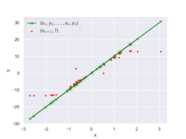
Figure 1: Plots showing examples of boundary values for different models. (Left) Full transformer 12L8AH model tested on $f(x)=9x$ and (Right) Transformer 12L8AH without MLP model trained on $D_{\cal I}=D_{\cal F}={\cal N}(0,1)$ and tested on $f(x)=10x$.

5.1 Comparison with larger fine-tuned and prompted LLMs

Figure 2: Attention maps for an ICL example for the task "every" of type $(x_{1},f(x_{1}),x_{2},f(x_{2}),...,x_{n})$, where the query $x_{n}$ is a big value.

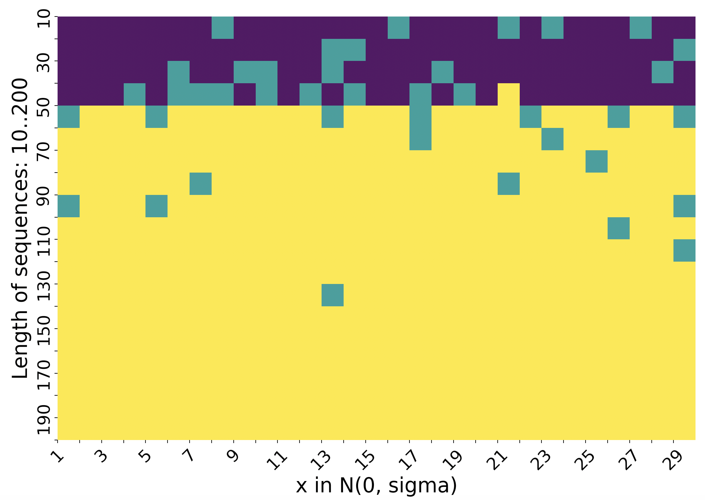
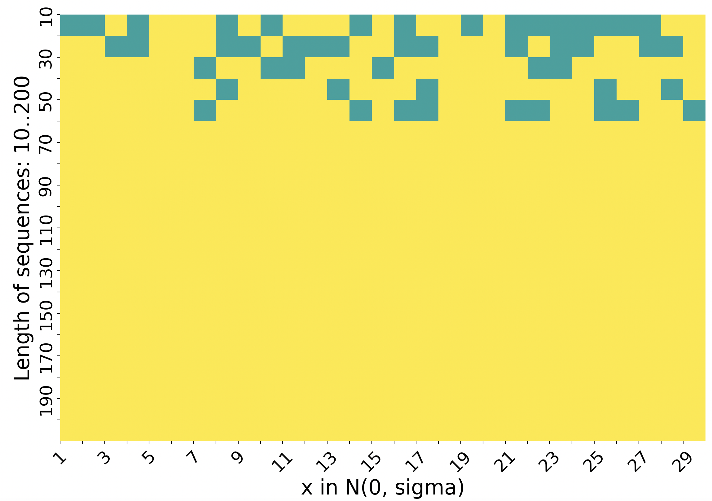
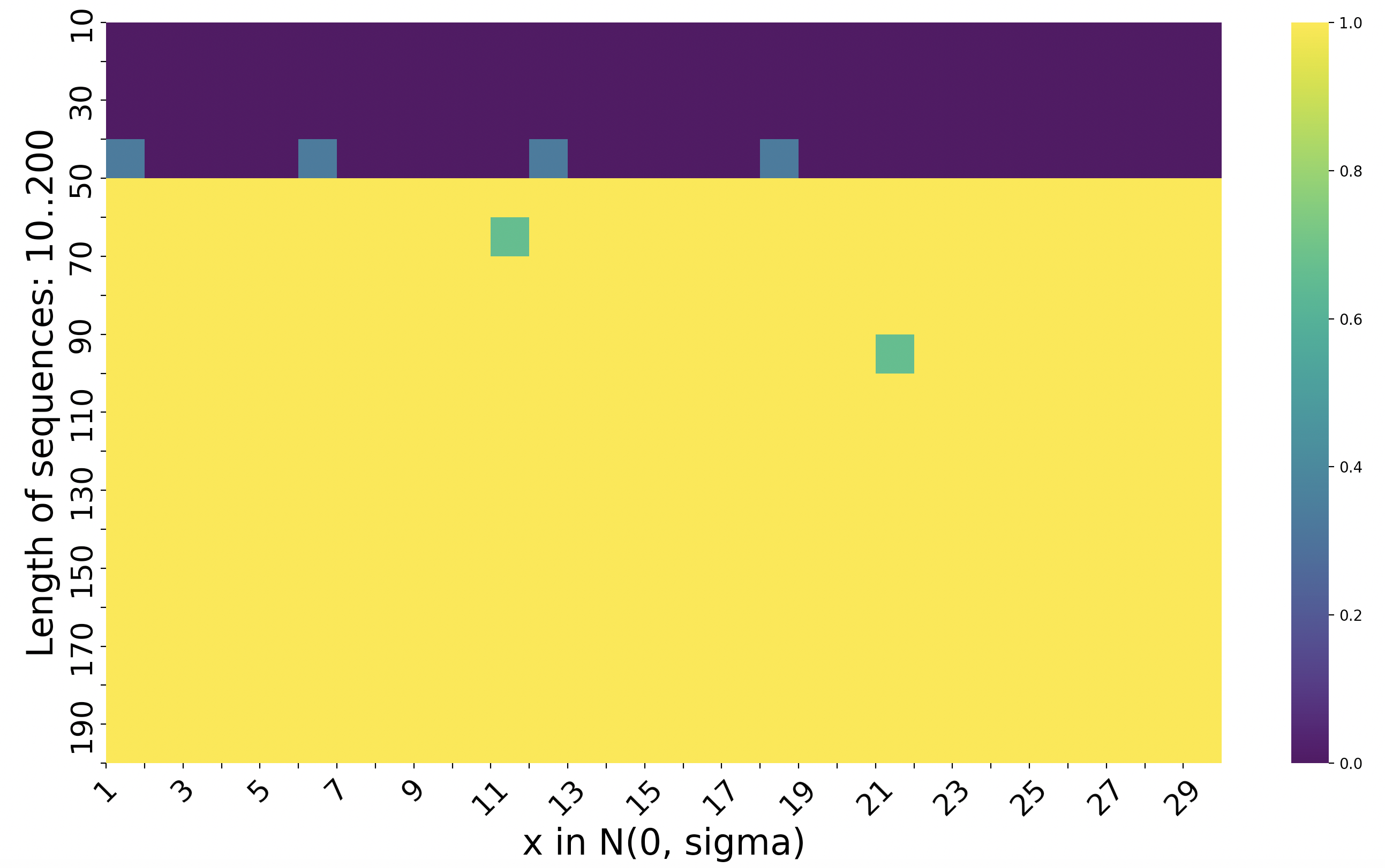
Figure 8: Heatmap showing the evolution of errors for the task "every" on "Pretrained Llama 3.3 70B" (First), "Pretrained Llama 3.1 8B" (Second) with 5 shot learning and finetuned on Llama 31 8B" (Third), on data in $D_{\cal I}={\mathcal{N}}(0,1)$ for lengths from 1 to 40 and tested in $D^{t}_{\cal I}={\mathcal{N}}(0,\sigma)$ for $\sigma\in\{1,...,10\}$ and lengths from 10 to 200.

Generalization from training data was a challenge not only for our smaller models but also for much larger ones. We evaluated performance on the quantification task using both fine-tuned (see Appendix A for details) and prompted versions of LLaMA 3.1 8B, as well as the prompted LLaMA 3.3 70B model. In a 5-shot setting, prompted LLaMA 3.1 8B failed to master numerical inputs from $D^{\text{test}}_{\cal I}$ and showed no generalization to longer sequences. LLaMA 3.3 70B performed better on numerical inputs drawn from distributions outside ${\mathcal{N}}(0,1)$ but, similarly, failed to generalize to longer sequence lengths. Interestingly, the fine-tuned LLaMA 3.1 8B was able to handle large numbers within a sequence, as shown in Figure 8, but still did not generalize beyond the sequence lengths seen during training.
We also tested the prompted LLaMA 3.3 70B on the linear function task with inputs and target functions sampled from $D_{\cal I},D_{\cal F}\sim{\mathcal{N}}(0,1)$. While the model sometimes appeared to assume linearity and apply a regression-like strategy, it still underperformed relative to our small models (see Table 1).

5.2 Ablation studies: the sources of ICL and limits to generalization

We looked at what might be responsible for ICL and its limitations. As with Olsson et al. (2022), we found that ICL was effective on our tasks even in models composed solely of attention layers, with no feedforward components (FF); these attention-only models performed comparably to their full transformer counterparts (see Figure 14). In contrast, small models consisting only of feedforward layers failed to perform ICL. This indicates that the attention mechanism is both necessary and sufficient for ICL on our tasks. As in Naim and Asher (2024), models without FF components also show boundary values, which means that boundary values originate from the multi-head attention itself.

We then examined various components of our models to identify the source of their generalization failures. To understand why the models struggled to generalize on the quantification task, we first tested whether they could correctly classify individual numbers in deviant sequences as positive or negative. The models performed well on this subtask, and so had the information needed to complete the quantification task successfully. But they could not use the information in the right way.

Given the importance of numerical representation in this task, we examined the way numbers were encoded. Since the quantification task depends on numerical magnitudes, and since large or rarely seen numbers can pose representational challenges, we used a linear embedding $Emb:x\mapsto x\cdot W$, for $(x,W)\in\mathbb{R}\times\mathbb{R}^{d}$. This mapping preserves numerical ordering simple and interpretable and maintains the ordering of magnitudes, such that if $|x|<|y|$ then $||emb(x)||<||emb(y)||$, where $||\cdot||$ denotes the vector norm. Crucially, this encoding mechanism did not introduce boundary effects. It preserved natural magnitude orderings and did not appear to contribute to the model’s failure on the quantification task.

5.3 The issues with Softmax

We then looked in more detail at the workings of the attention matrix. To recall the basics of attention, let $\vec{e}^{l}=(e_{1}^{l},...,e_{n}^{l})$ be the input embeddings processed by the multi-head attention mechanism at layer $l$, where $e_{i}^{l}$ denotes the embedding of the $i$-th token in that layer. Each attention head $h$ in layer $l$ is parameterized by Query, Key, and Value weight matrices, denoted as $Q^{h,l},K^{h,l}$, and $V^{h,l}$, respectively. The dimension $d_{k}$ corresponds to the embedding size divided by the number of heads. The output of each attention head $h$ in a layer $l$ is a sequence of vectors $(C_{1}^{h,l},C_{2}^{h,l},...,C_{n}^{h,l})$ where each:

$${C_{i}^{h,l}=\sum^{n}_{j=1}\left(\mathrm{softmax}\left(\frac{(Q^{h,l}e_{i}^{l})^{\top}(K^{h,l}e_{j}^{l})}{\sqrt{d_{k}}}\right)\right)V^{h,l}e_{j}^{l}}$$ (3)

The primary role of an attention head is to refine the embedding of each input $e^{l}_{i}$ by incorporating contextual information from surrounding tokens. However, once the gap between the input values $e^{l}_{j}$ in the argument of the Softmax operator in equation 3 become large —specifically, when the gap between the largest value and the others exceeds a threshold (a difference of 4 is typically sufficient), the resulting Softmax weights rapidly saturate. In such cases, the attention weight assigned to the maximum value approaches 1, while the weights for all other values approach 0. As a result, the model focuses almost entirely on a single token, the one associated with the maximum value, while effectively ignoring the rest of the context.

$$C_{i}^{h,l}=V^{h,l}e_{j_{0}}^{l}$$ (4)

As our embedding function is linear, if $|x|$ is significantly larger than $|y|$, then $||e(x)||$ will be significantly larger than $||e(y)||$ and so large differences in number inputs will have the effect noted in equation 4.

It is important that the values in deviant sequences that yield equation 4 come from inputs that the model has seldom seen in training, because then the $Q$ and $K$ matrices cannot have been trained to handle them, ensuring that the large $x_{j}$ affects Softmax as in equation 4.

We verified these predictions by examining the outputs from the attention matrices of the last layer of the model in the quantification task. Figure 2 confirms experimentally what we showed mathematically: in the case of a significant gap between values, the attention layer puts all the weight on the largest value in the sequence; the other elements in the sequence which determined the truth value for LABEL:every are ignored. In Figure 2, the model focuses only on the maximum value $70$ and falsely predicts the sequence as all positive based only on this value.

With significant differences in input values, the Softmax function increasingly resembles a Hardmax operation , assigning a weight close to 1 to the largest element and weights near 0 to all others. In addition, it makes the score of negative values tend towards 0 due to the exponential. Significant differences that can affect Softmax occur not only with numerical inputs but with linguistic tokens. Tokens from OpenWebtext can have such differences (see Figure 9 in Appendix F).

Training on distributions with a much larger range of elements like $D_{\cal I}={\mathcal{N}}(0,10)$ or $D_{\cal I}={\mathcal{N}}(0,100)$ improved model performance on deviant sequences but significantly increased squared errors on ${\mathcal{N}}(0,\sigma)$ for small $\sigma$. This training gave the $Q$ and $K$ matrices small weights to compensate. Since Softmax makes the scores on a set of very small values constant, the model becomes less accurate. Additionally, all models suffered in performance once the out of distribution elements $x_{i}$ in deviant inputs became sufficiently large.

In the linear functions task, when a value $x_{i}$ in the sequence input to the attention mechanism is larger than the other elements of the sequence and other elements in its training, mathematically Softmax should assign $x_{i}$ probability $1$ and all other elements in the sequence probability $0$. This affect models performances. Consider, for example, a 12L8AH model’s predictions for $f(x)=x$ with this input sequence with $x_{1}=100$: $[100,-1.09,0.78,0.26,0.42]$. The model’s predictions are: $[-1.21,-0.28,2.15,0.96,0.65]$. Given this large value, model fails to reasonably approximate the function.

Softmax treats comparatively large values as very significant. This makes sense in the abstract; a large value in the attention mechanism intuitively signals a strong statistical correlation in context sensitive aspects of meaning Asher (2011); Softmax amplifies this value. However, in our tasks this is problematic. While an input token representing a large number may carry higher semantic magnitude than surrounding tokens, its importance for the task is not necessarily disproportionately greater. Our tasks require the model to look at many tokens in the context; but with deviant sequences, Softmax prevents the models from doing this.

6 Some alternatives to Softmax

Attempting to remedy the deficiencies of Softmax we observed, we investigated a hybrid attention mechanism. We partitioned the attention heads such that half utilized Softmax-based scoring, while the remaining half employed uniform averaging over all tokens. This design, we thought, would preserve contextual breadth, reduce the risk of focusing to specific tokens, and also increase the model’s expressiveness through multiple scoring functions. However, empirical results showed that this approach did not yield expected improvements in performance. We further extended this approach by experimenting with four distinct known scoring functions (tanh, average, ReLU, and $x^{2}$), assigning two heads to each (For detailed results see Table 1). This approach improved over than Softmax on ${\cal N}(0,1)$ but was less good elsewhere. It did not solve the observed problems either. We also tested CosFormer Qin et al. (2022) and SA-Softmax Zheng et al. (2025). Both performed worse than Softmax in our experiments.

7 Solution: Signed scaled averaging (SSA)

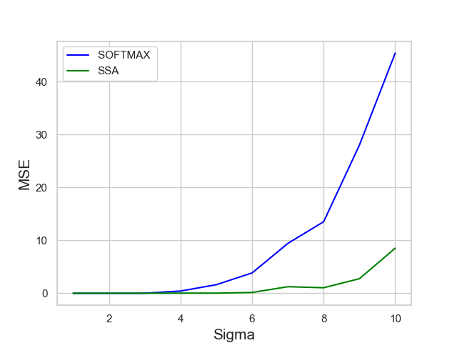
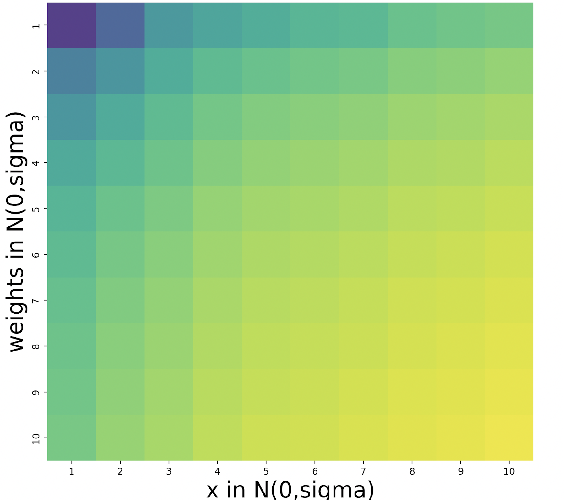
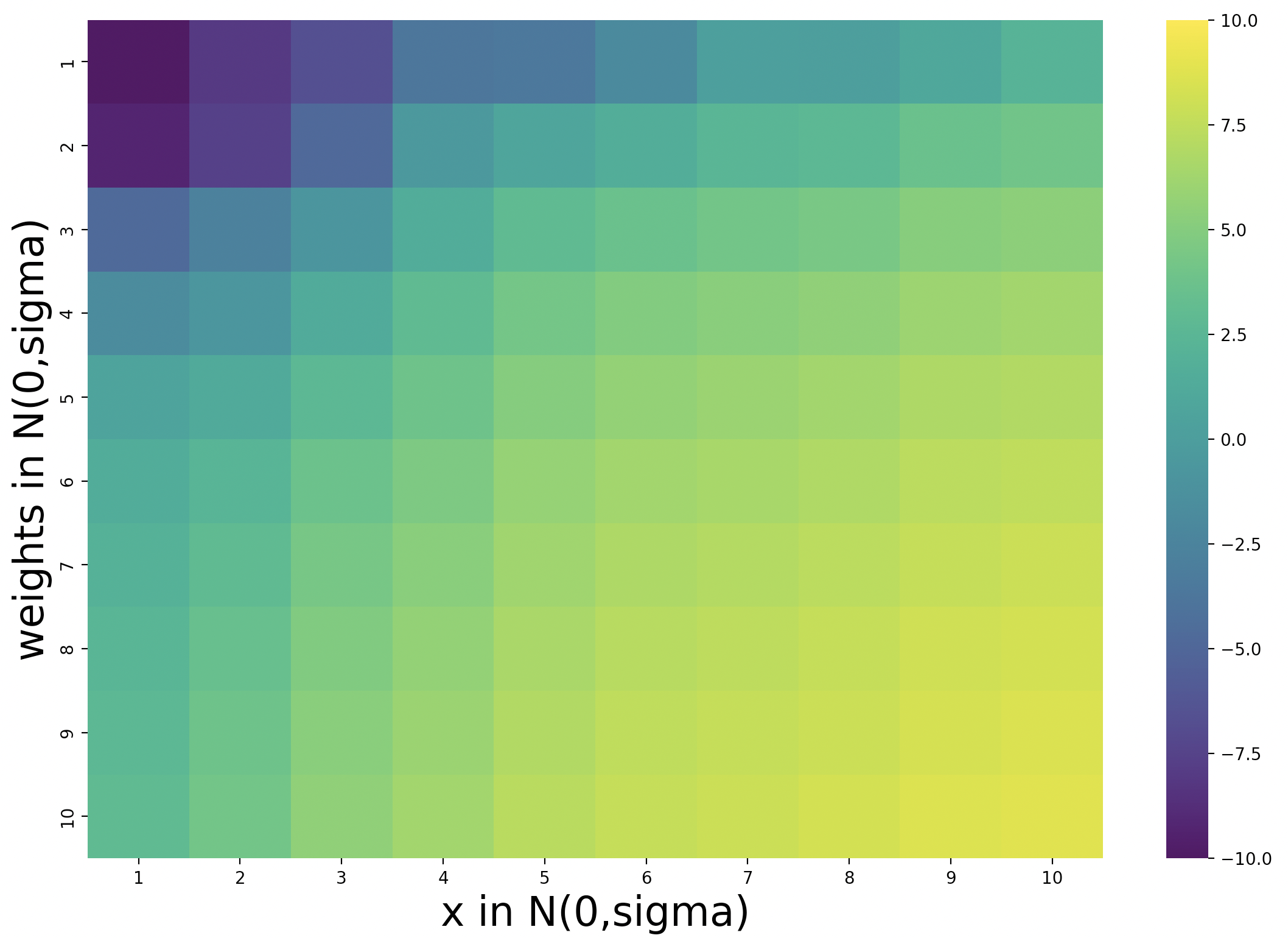
Figure 3: (Left) Comparison plot showing the evolution of MSE for SSA and Softmax-based models (12L8AH) with $D_{\cal F},D_{\cal I},D^{test}_{\cal I}\sim{\mathcal{N}}(0,1)$ and $D^{test}_{\cal F}$ and varying $D_{\cal F}^{test}\sim{\mathcal{N}}(0,\sigma)$. The heatmap shows the evolution of logarithm of MSE for the Softmax (Middle) and SSA (Right) model when varying both $D^{test}_{\cal I}$ and $D^{test}_{\cal F}$.

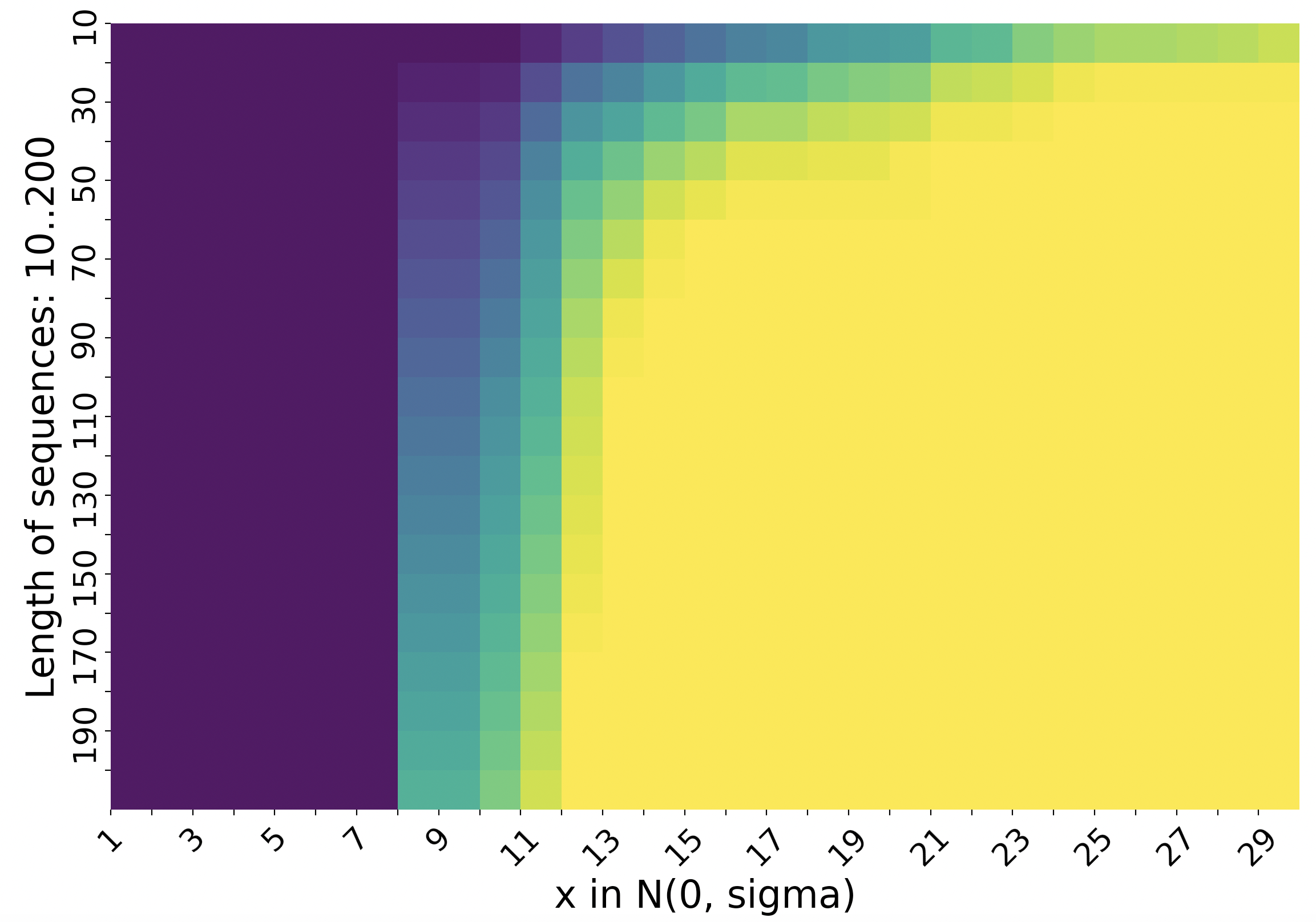
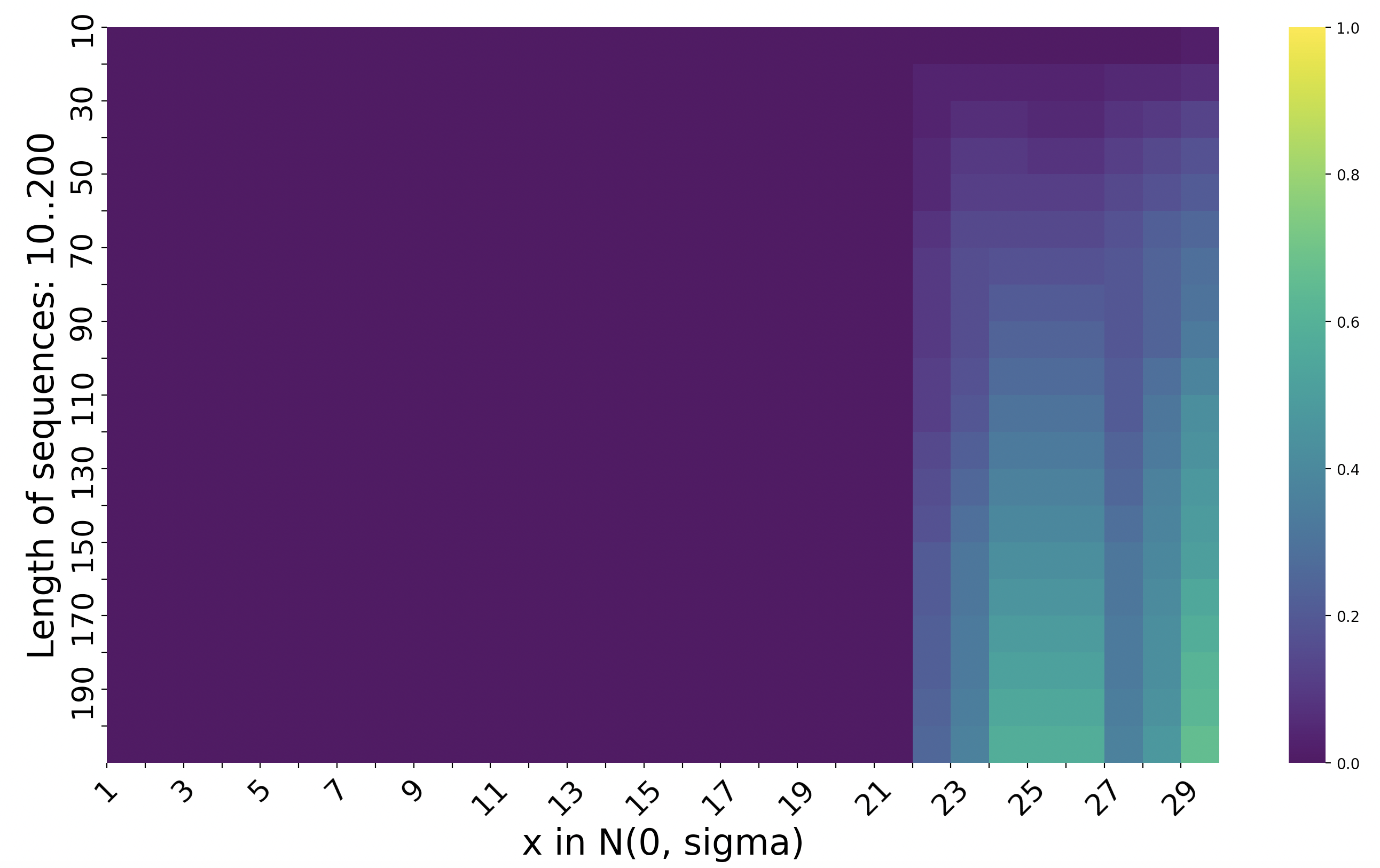
Figure 4: Heatmaps showing the evolution of errors for the 12L8AH model with Softmax (Left) and SSA (Right) on the "every" task. Model was trained on data in $D_{\cal I}={\mathcal{N}}(0,1)$ for lengths from 11 to 40 and tested in $D^{test}_{\cal I}={\mathcal{N}}(0,\sigma)$ for $\sigma\in\{1,...,10\}$ and lengths from 10 to 200 for each task. Yellow represents a much higher error rate than purple.

models $\backslash$ $\sigma$	1	2	3	4	5	6	7	8	9	10
SSA	$4\times 10^{-5}$	$3\times 10^{-4}$	$10^{-3}$	$0.02$	$0.02$	$0.15$	$1.24$	$1.04$	$2.74$	$8.5$
Softmax	$8\times 10^{-5}$	$3\times 10^{-4}$	$6\times 10^{-3}$	$0.42$	$1.62$	$3.84$	$9.42$	$13.51$	$27.99$	$45.35$
SOFT/AVG	$7\times 10^{-5}$	$3\times 10^{-3}$	$0.30$	$1.22$	$2.91$	$7.52$	$10.32$	$22.97$	$38.97$	$60.03$
4 Scoring fts	$5\times 10^{-5}$	$3\times 10^{-3}$	$0.34$	$1.33$	$3.18$	$8.28$	$10.99$	$26.31$	$42.42$	$70.33$
CosFormer	$2\times 10^{-4}$	$5.6\times 10^{-3}$	$0.43$	$2.07$	$5.10$	$12.54$	$16.91$	$46.68$	$66.22$	$91.02$
SA-Softmax	$6\times 10^{-5}$	$2.8\times 10^{-3}$	$0.37$	$1.83$	$3.83$	$11.94$	$13.72$	$39.29$	$58.43$	$80.31$
Llama 3.3 70b	$2\times 10^{-3}$	$5.50$	$3.16$	$13.71$	$18.21$	$23.91$	$28.99$	$33.51$	$40.25$	$48.02$

Table 1: Comparison showing the evolution of squared errors for models tested on $x\in D^{t}_{\cal I}={\mathcal{N}}(0,1)$ and weights $a,b\in D^{t}_{\cal F}={\mathcal{N}}(0,\sigma)$. SSA, CosFormer and Softmax are 12 layer, 8 attention head full transformer models.

linguistic probe	MLM				Holistic
	Softmax	SSA 1.1	SSA 1.5	SSA 2	Softmax	SSA 1.1	SSA 1.5	SSA 2
agreement_Det_N-across_1_adj	75.35	76.7	73.5	73.3	56.45	57.55	54.95	56.40
agreement_subject_verb-across_PP	56	55.75	58.95	65.95	51.55	51.25	51.35	52.05
agreement_subject_verb-across_RC	55.5	55.75	57.7	61.55	51.9	52.15	52.15	50.05
agreement_subject_verb-in_Q+aux	76.5	69.6	79.0	70.45	50.1	48.95	49.95	49.05
anaphor_agreement-pronoun_gender	48.1	50.25	51.45	53.7	52.7	49.9	52.75	52.75
argument_structure-dropped_arg	79.65	74.65	74.65	85.55	70.7	80.9	72.85	75.85
argument_structure-swapped_args	83.3	83.1	92.0	88.0	62.45	58.4	53.3	33.15
argument_structure-transitive	53.44	55.3	53.85	57.2	55.3	53.7	56	55.6
binding-principle_a	78.25	79.55	87.9	80.2	66.4	68.2	75.0	68.85
case-subjective_pronoun	85.55	86.5	89.7	91.75	67.55	81.1	59.6	46.9
ellipsis-n_bar	60.75	56.25	53.3	53.45	35.15	43.3	34.7	33.65
filler-gap-wh_question_object	91.7	90.65	89.4	87.15	91.9	89.15	91.05	80.3
filler-gap-wh_question_subject	79.2	79.1	83.3	68.25	65.3	89.25	89.25	48.55
irregular-verb	70.05	64.85	78.3	69.2	50.15	58.8	72.1	52.5
local_attractor-in_question_with_aux	85.45	87.35	81.85	85.0	87.8	89.7	87.65	86.1
quantifiers-existential_there	91.3	86.6	85.25	76.25	86.15	87.3	80.9	85.15
quantifiers-superlative	71.2	76.1	83.95	65.25	51.2	47.45	38.9	31.85
OVERALL	73.01	72.23	74.94	72.48	61.92	65.12	63.08	56.39

Table 2: BabyBERTa Model performance trained from scratch on AO-CHILDES with Softmax and three settings of SSA, evaluated with the holistic metric on various linguistic probes from Huebner et al. (2021). PP: prepositional phrase; RC: relative clause; Det: determiner; N: noun. arg: argument.

Having found that previously proposed alternatives to Softmax did not lead to performance improvements in our settings, we explored a new approach. Inspired by $\lim\limits_{n\to+\infty}(1+\frac{x}{n})^{n}=e^{x}$, we replaced the exponential in the scoring function by a parametrized form: $x\mapsto(1+b|x|)^{{\rm sgn}(x)n}$ where $b>0$ is a trainable parameter and $n>1$ a fixed exponent (we typically set $1.1$ or $1.5$, though it can also be learned). This formulation allows us to approximate the exponential while controlling its sharpness. It allows interpolation between linear and exponential behaviors. By training $b$ and selecting (or training) different values of $n$, the model gains flexibility: it can mimic Softmax-like behavior when appropriate, while also tempering the dominance of large input values. This provides a better balance between focus and diversity in attention.
For positive inputs, the function behaves similarly to Softmax, but with a slower growth that prevents early Hardmax saturation. For negative inputs, the presence of $sign(x)$ ensures the score decays toward zero, like Softmax, but less abruptly. This allows the model to still consider low-scoring elements rather than suppressing them entirely.
For a vector $z=(z_{1},\cdots,z_{K})\in\mathbb{R}^{K}$ with parameters $b>0$ and $n>1$, we replace Softmax by:

$${\rm score}(z_{i})=\frac{(1+b|z_{i}|)^{{\rm sgn}(z_{i})n}}{\sum^{K}_{k=1}(1+b|z_{k}|)^{{\rm sgn}(z_{k})n}}$$ (5)

Substituting Softmax with SSA improves our models’ generalization ability dramatically, both with respect to the length of test sequences and the magnitude of deviant inputs. The heat map in Figure 4 shows the improvement for the predictions of our standard full transformer model with 12L8AH with SSA on the right compared to the same model with Softmax on the left for the every task. The improvement with SSA on the "some" task is also significant (see Appendix C).

Our best 12L8AH model also dramatically increased performance in learning linear functions on out-of-distribution data for function parameters when we used SSA instead of Softmax as scoring a function (see Figure 3). SSA was the best scoring function we tested on our tasks.

8 SSA and NLP tasks

To assess the applicability of SSA beyond our synthetic tasks and to more complex natural language processing scenarios, we trained three GPT-2 models (each with 134 million parameters) from scratch on the OpenWebText corpus (9B tokens) for 20,000 steps. One model used the standard Softmax scoring function, while the other two employed SSA: one with a fixed exponent $n=1.5$, and the other with $n$ treated as a trainable parameter. We evaluated model performance using perplexity, as this is a widely accepted metric for language modeling tasks and provides a direct, quantitative comparison across models trained with different scoring functions.

The model with trainable SSA had a loss of 3.19 and SSA 1.5 model had a loss of 3.15 after 20k training steps, instead of 3.27 for the Softmax. Trainable SSA had a minimum loss of 2.76 after 26k steps. While the baseline Softmax model achieved a perplexity of 31.73, The SSA 1.5 and trainable SSA models achieved a significantly lower perplexity of 27.71 and 29.35 respectively, all on 20K step training. All models also share the same architecture and parameter count. SSA’s better perplexity is thus compelling. Trainable SSA achieved a perplexity of 27.21 after 30K steps.

In a further study, we trained multiple variants of the BabyBERTa model (Huebner et al., 2021) on the AO-CHILDES dataset: one using the standard Softmax scoring function, and three separate models using SSA with fixed exponents $n=1.1$, $n=1.5$, and $n=2$, respectively. BabyBERTa has demonstrated performance comparable to much larger RoBERTa models on linguistic probing tasks, despite being trained on substantially smaller datasets (Huebner et al., 2021). For these experiments, we used the BabyBERTa encoder-only model, as encoder architectures have been shown to perform better on grammar classification tasks involving masking. We evaluated our four models on 17 of the linguistic probes from (Huebner et al., 2021). We used two metrics for testing on linguistic probes: holistic scoring Zaczynska et al. (2020) which measures the correct prediction of all masked elements, and masked language model (MLM) scoring Salazar et al. (2020), which assesses the accuracy of predicting correct tokens versus distractors. On the stricter holistic method, SSA 1.1 BabyBERTa averaged over 2 percentage points higher than Softmax BabyBERTa. SSA1.1 had the highest score over the other models in 8 probes. Softmax only beat the SSA models on 4 probes (see Table 2). On the MLM metric, SSA 1.5 averaged almost 2 percentage points higher than Softmax, SSA 1.1 and SSA 2. Softmax BabyBERTa scored highest on 3 probes while SSA 1.5 and SSA 2 scored best on six of the probes.

9 Conclusion

The literature has noted that small transformer models struggle to generalize effectively to out-of-distribution data, a limitation we have also empirically confirmed. We identified the Softmax scoring function in the attention mechanism as a factor contributing to this challenge and introduced a novel scoring method that significantly improves the performance of small transformer models on both mathematical and NLP tasks. SSA enhances a model’s ability to predict linguistic structure, offering improved performance without increasing model complexity. The fact that SSA is parametrizable and adaptable to different tasks adds to its attractiveness and shows its advantages over a one-size-fits-all scoring function like Softmax.

Limitations

Due to hardware and data limitations, we could not train all the SSA tasks with the parameter $n$ as trainable. We were also unable to train models larger than 124M parameters from scratch with SSA.

While SSA provides noticeable improvements in generalization, it does not fully address all the shortcomings of the attention mechanism. In particular, our heatmaps indicate that SSA struggles to generalize in scenarios where both the input $x_{i}$ and the test-time function distribution $D^{\text{test}}_{\mathcal{F}}$ diverge significantly from the training distribution $D_{\mathcal{F}}$.

Thus, SSA does not address the fact that, as we have noted above, the simple mathematical structure of the attention mechanism conflates the value of tokens with their importance for the particular task.

Appendix A Training details

Additional training information: We use the Adam optimizer Diederik (2014) , and a learning rate of $10^{-4}$ for all models.
Computational resources: We used Nvidia A-100 GPUs to train the different versions of transformer models from scratch and used Nvidia Volta (V100 - 7,8 Tflops DP) GPUs for the fine-tuning of LLaMA 3.1 8B involved in these experiments.

Fine-tuning LLaMA 3.1 8B was fine tuned on 26000 randomly generated sequences $S$ progressing from 1 to $40$ for 2 epochs using LoRA (Hu et al., 2022). The input values were drawn from ${\mathcal{N}}(0,1)$. At test time, we were only able to run a few sequences for each possible we examined sequence lengths from 10 to 200 and number distributions from ${\cal N}(0,\sigma)$ for $1\leq\sigma\leq 30$. This meant that we could only run a few test batches, since we need to look at 600 total pairs for each task. We averaged the prediction errors on the each $(S^{\text{test}},D^{\text{test}}_{\cal I})$ possibility.

For our attempted fine-tuning of LLaMA 3.1 8B on the function task, we set the input sequence to be of the form $(x_{1},f(x_{1}),x_{2},f(x_{2}),....,x_{n})$ requiring that the output be of the form $f(x_{n})$, a single numerical value. The model returned a list of values $(w_{1},w2,...)$. It failed to capture the basic input and output pattern.

Appendix B Some base functions for SSA

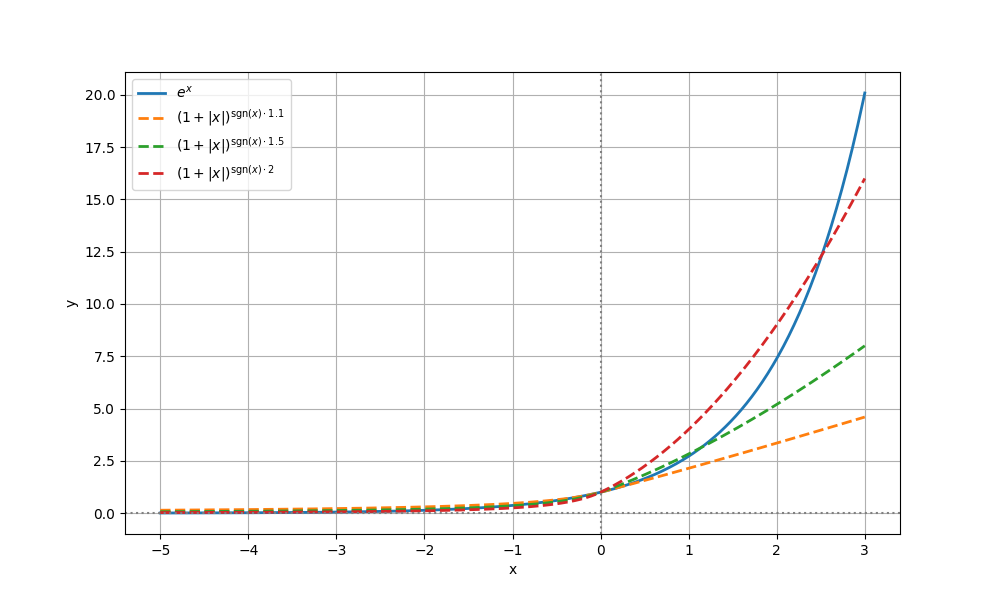
Figure 5: Figures showing plots for the base function $(1+b|x|)^{sgn(x)n}$ for SSA with $b=1$ and $n=\{1.1,1.5,2\}$

Appendix C Heat map for the "some" task with SSA for model trained from scratch

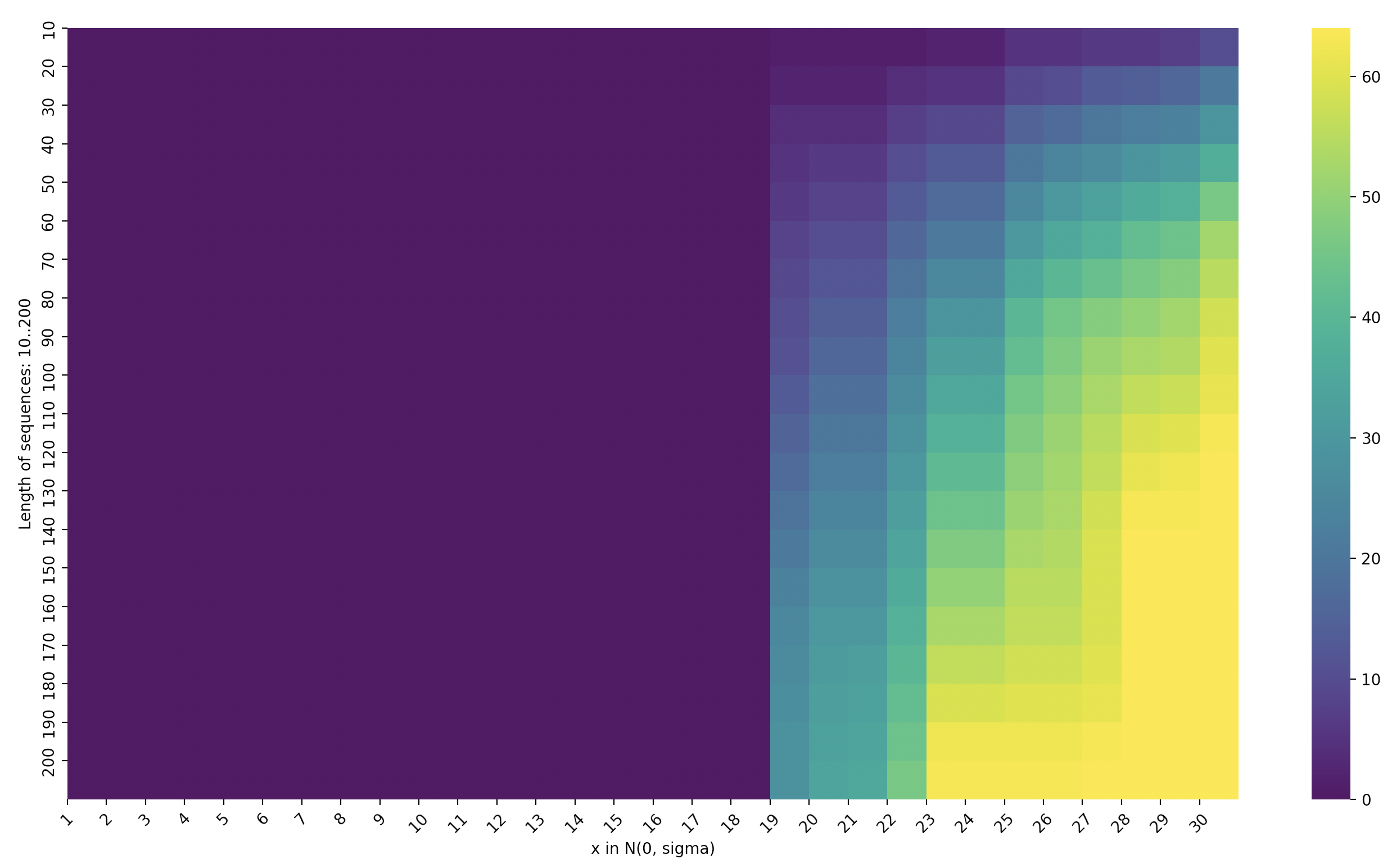
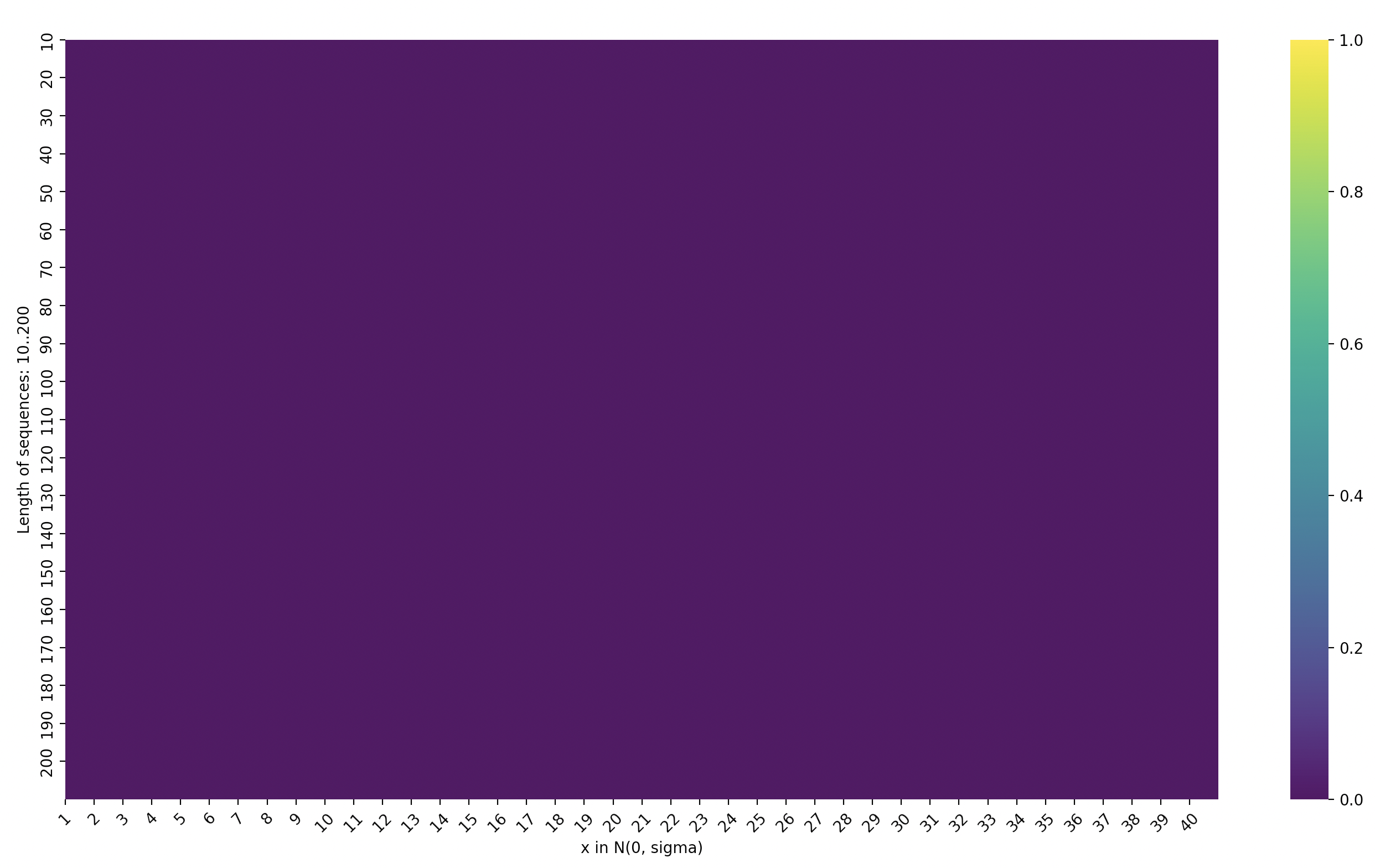
Figure 6: Heatmap showing the evolution of errors for the task "some" trained on data in $D_{\cal I}={\mathcal{N}}(0,1)$ for lengths from 11 to 40 and tested in $D^{\text{test}}_{\cal I}={\mathcal{N}}(0,\sigma)$ for $\sigma\in\{1,...,10\}$ and lengths from 10 to 200. The first figure is for the Softmax-based model and the second with SSA.

Appendix D Heat map for the "some" task with pretrained and finetuned models

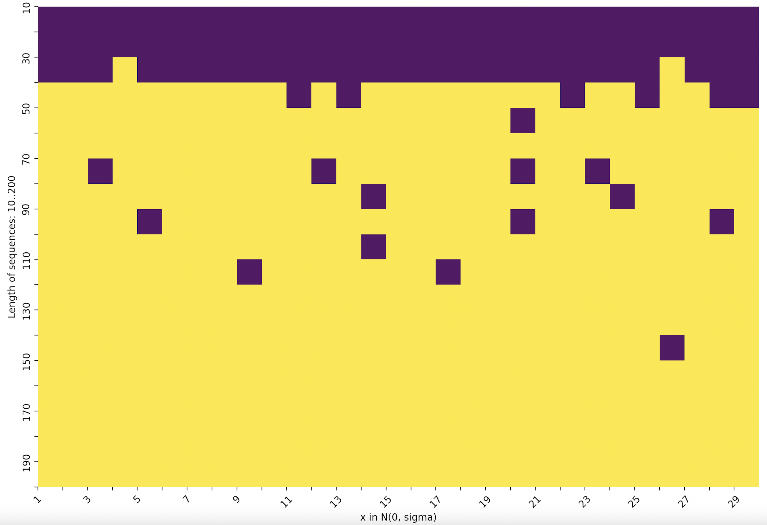
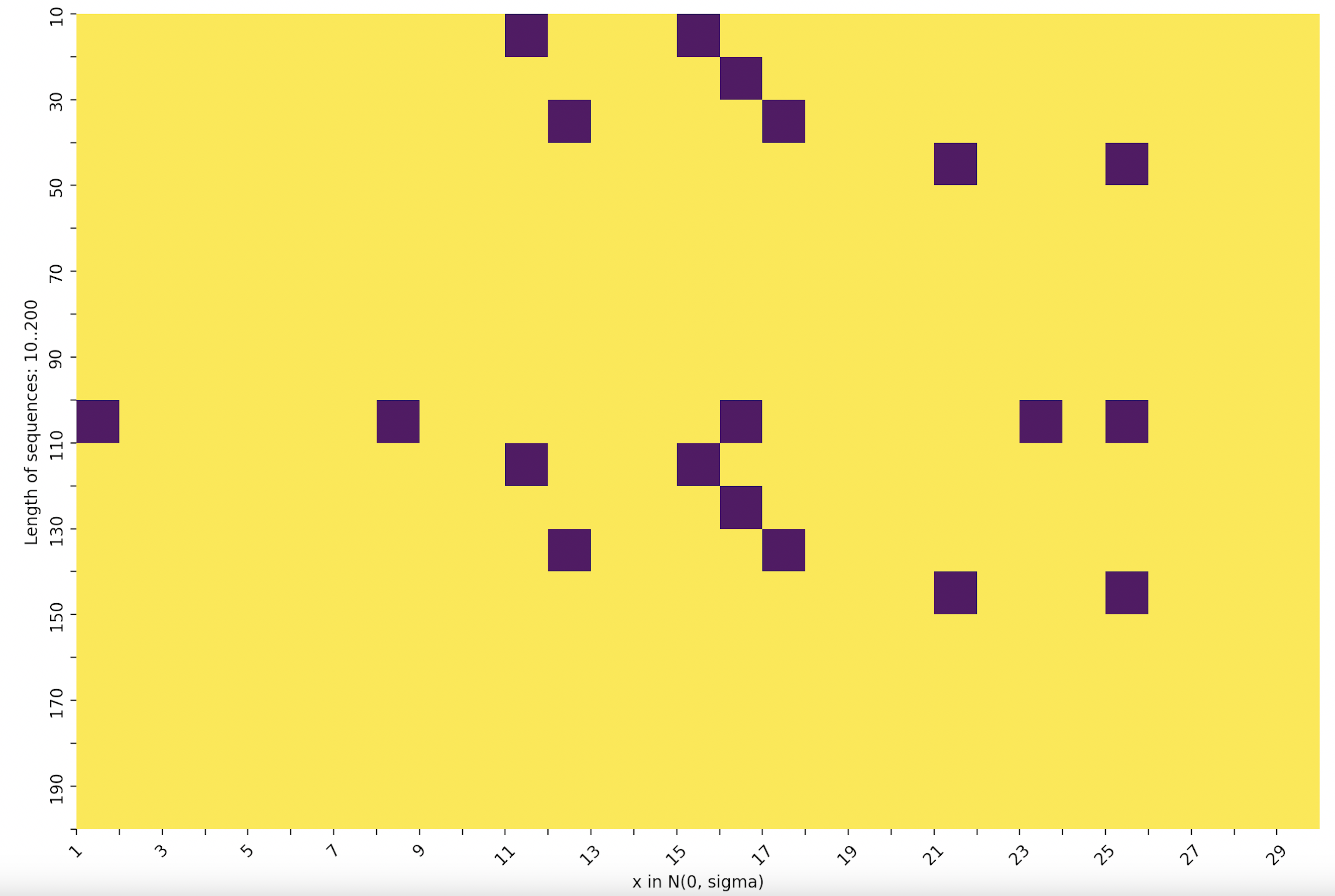
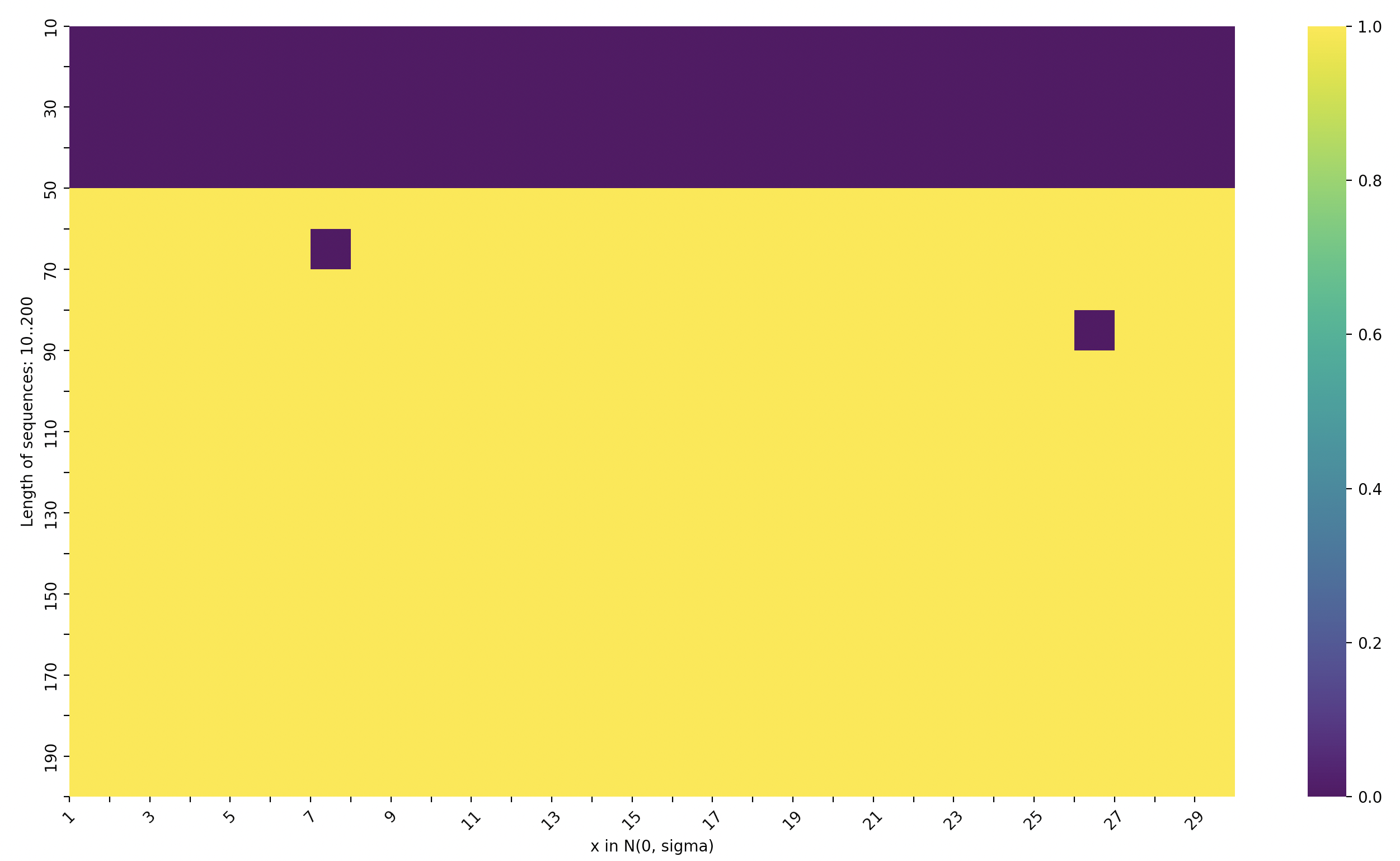
Figure 7: Heatmap showing the evolution of errors for the task "some" on different models "Pretrained Llama 3.3 70B", "Pretrained Llama 3.1 8B" and finetuned on Llama 31 8B", respectively from top to bottom on data in $D_{\cal I}={\mathcal{N}}(0,1)$ for lengths from 11 to 40 and tested in $D^{t}_{\cal I}={\mathcal{N}}(0,\sigma)$ for $\sigma\in\{1,...,10\}$ and lengths from 10 to 200.

Appendix E Heat map for the "every" task with pretrained and finetuned models

Appendix F Repartition of token norms in the OpenWebText

Figure 9: Plot showing how many tokens have a norm of value x, for OpenWebText using GPT-2 Tokenizer. The x-axis is token embedding norm and the y-axis is token count (log scale)

Appendix G Example showing that Boundary values behaviors

Figure 10: Plots for model 12L8AH, trained on $D_{\cal I},D_{\cal F}\sim{\mathcal{N}}(0,1)$ for $f(x)=x$ for high values (First) of $x$ and $f(x)=10x$ for normal (Second) then for low values of $x$ (Third)

models $\backslash$ $\sigma$	1	10	20	30	40	50	60	70	80	90	100
12L8AH	6.4e-05	0.05	0.25	0.50	0.82	1.21	1.66	1.87	2.02	2.14	2.20

Table 3: Table showing the influence of deviant inputs: Comparison showing the evolution of squared errors for models tested on $x\in D^{t}_{\cal I}={\mathcal{N}}(0,1)$, except the first element $x_{0}\in D^{t}_{\cal I}={\mathcal{N}}(0,\sigma)$ and weights $a,b\in D^{t}_{\cal F}={\mathcal{N}}(0,1)$.

models $\backslash$ $\sigma$	1	2	3	4	5	6	7	8	9	10
1L1AH	0.1	0.8	5.1	13.1	26.9	39.7	53.0	84.8	120.0	153.2
1L2AH	0.1	0.8	5.3	14.4	29.8	41.1	55.0	93.8	120.4	159.2
1L4AH	0.0	0.2	2.7	8.7	19.9	32.0	42.8	64.5	92.3	131.2
2L1AH	0.0	0.1	2.0	4.9	13.7	27.0	36.1	64.9	99.0	134.0
2L2AH	0.0	0.0	1.6	3.2	9.3	25.5	32.0	61.1	92.9	127.8
2L4AH	0.0	0.0	0.9	2.6	7.5	19.3	27.3	51.8	90.2	119.4
3L1AH	0.0	0.0	0.9	3.0	8.2	16.8	24.4	48.4	76.7	113.2
3L2AH	0.0	0.0	0.7	2.3	6.5	15.9	22.5	43.1	74.0	102.5
3L4AH	0.0	0.0	0.6	1.9	5.5	13.8	20.4	42.2	70.3	100.4
6L4AH	0.0	0.0	0.5	1.6	4.6	11.6	16.8	33.7	58.3	87.9
12L8AH	0.0	0.0	0.3	1.1	2.9	7.9	11.9	28.3	46.9	73.5
18L8AH	0.0	0.0	0.2	1.1	2.8	7.1	10.3	22.9	40.3	64.6
$2Al32AH$	1.17	2.64	3.47	5.01	7.88	16.85	24.1	40.98	66.04	95.03
$12Al8AH$	0.0	0.0	0.41	1.70	3.92	10.40	14.04	30.20	52.69	79.13

Table 4: Comparison to show the evolution of squared error over different models. $D_{\cal I}^{test}\sim N(0,1)$.

Appendix H Prompts used for tests on pretrained models

The prompts are in the Figures 11, 12 and 13.

Figure 11: Prompt used for the task "every"

Figure 12: Prompt used for the task "some"

Figure 13: Prompt used for the task "Linear Function"

Appendix I Example of an output generated by a fine-tuned Llama 3.1 8b on Linear functions

Llama 3.1 8b fine-tuned on Linear Function did not understand the task and was not consistent even with the size of the output generated, which was different from an example to another. Here is an example of the generated output $[1.33,0.79,2.61,0.0,0.9]$.

Appendix J Error values for different models

To ensure that comparisons between models are meaningful, for each ${\mathcal{N}}(0,\sigma)$, we set a seed when generating the 100 random linear functions, ensuring that each model sees the same randomly chosen functions and the same set of prompting points $x_{i}$.

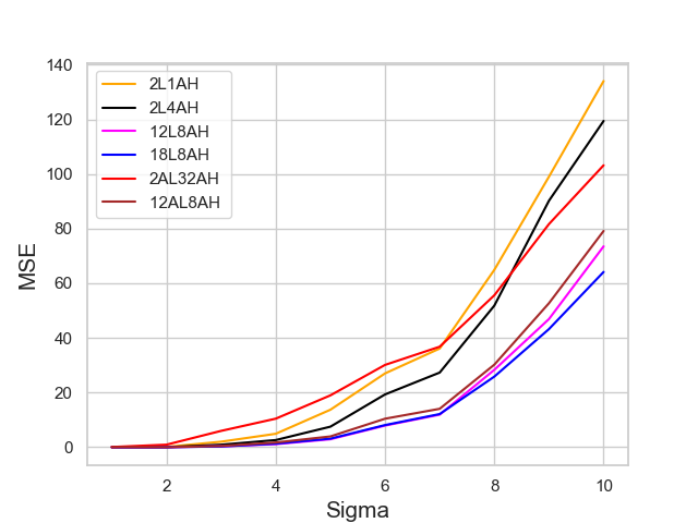
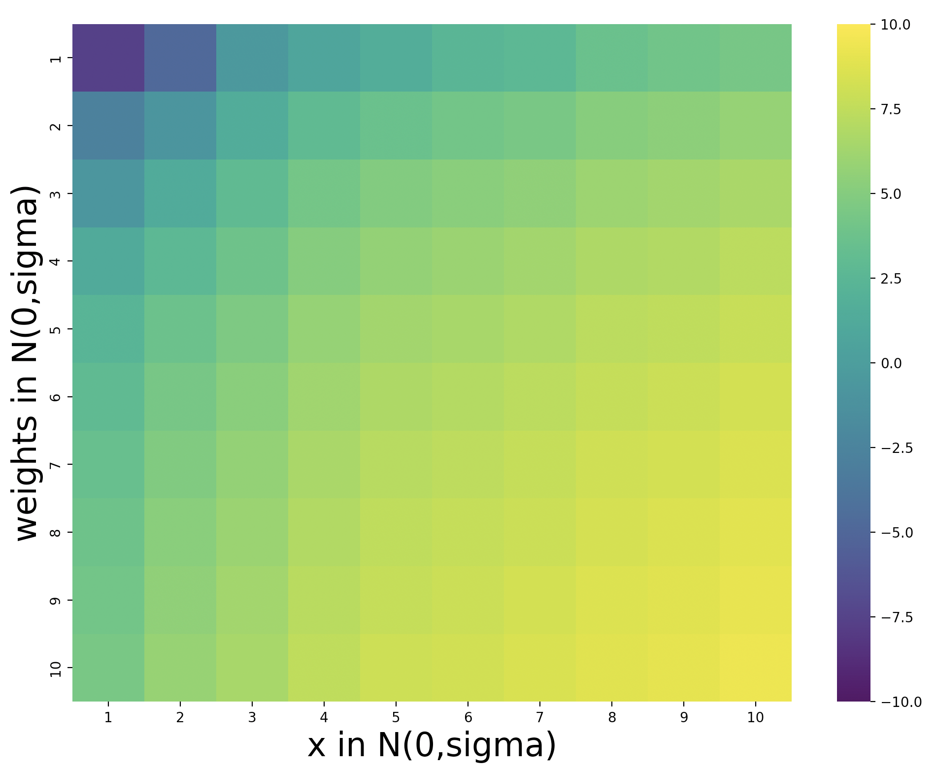
Figure 14: Evolution of MSE for various models with $D_{\cal F},D_{\cal I},D^{test}_{\cal I}\sim{\mathcal{N}}(0,1)$ and $D^{test}_{\cal F}\sim{\mathcal{N}}(0,\sigma)$ for various $n$. The heatmap shows error evolution when varying $D^{test}_{\cal I}$ and $D^{test}_{\cal F}$

.

The heatmap on the right in Figure 14 shows how our models generalized outside of the training distributions $D_{\cal F},D_{\cal I}\sim{\mathcal{N}}(0,1)$. Shifts both in $D^{test}_{\cal I}$ from $D_{\cal I}$ and in $D^{test}_{\cal F}$ from $D_{\cal F}$ prompted performance to degrade as can be seen in Figure 14. For error values on various distributions and models see Table 4 in Appendix J.

References

- Asher (2011) Nicholas Asher. 2011. Lexical Meaning in Context: A web of words. Cambridge University Press.
- Asher et al. (2023) Nicholas Asher, Swarnadeep Bhar, Akshay Chaturvedi, Julie Hunter, and Soumya Paul. 2023. Limits for learning with large language models. In 12th Joint Conference on Lexical and Computational Semantics (*Sem). Association for Computational Linguistics.
- Bhattamishra et al. (2023) Satwik Bhattamishra, Arkil Patel, Phil Blunsom, and Varun Kanade. 2023. Understanding in-context learning in transformers and llms by learning to learn discrete functions. arXiv preprint arXiv:2310.03016.
- Brown et al. (2020) Tom Brown, Benjamin Mann, Nick Ryder, Melanie Subbiah, Jared D Kaplan, Prafulla Dhariwal, Arvind Neelakantan, Pranav Shyam, Girish Sastry, Amanda Askell, and 1 others. 2020. Language models are few-shot learners. Advances in neural information processing systems, 33:1877–1901.
- Chaturvedi et al. (2024) Akshay Chaturvedi, Swarnadeep Bhar, Soumadeep Saha, Utpal Garain, and Nicholas Asher. 2024. Analyzing Semantic Faithfulness of Language Models via Input Intervention on Question Answering. Computational Linguistics, pages 1–37.
- Diederik (2014) P Kingma Diederik. 2014. Adam: A method for stochastic optimization. (No Title).
- Dong et al. (2022) Qingxiu Dong, Lei Li, Damai Dai, Ce Zheng, Jingyuan Ma, Rui Li, Heming Xia, Jingjing Xu, Zhiyong Wu, Tianyu Liu, and 1 others. 2022. A survey on in-context learning. arXiv preprint arXiv:2301.00234.
- Garg et al. (2022) Shivam Garg, Dimitris Tsipras, Percy S Liang, and Gregory Valiant. 2022. What can transformers learn in-context? a case study of simple function classes. Advances in Neural Information Processing Systems, 35:30583–30598.
- Giannou et al. (2024) Angeliki Giannou, Liu Yang, Tianhao Wang, Dimitris Papailiopoulos, and Jason D Lee. 2024. How well can transformers emulate in-context newton’s method? arXiv preprint arXiv:2403.03183.
- Hu et al. (2022) Edward J Hu, Yelong Shen, Phillip Wallis, Zeyuan Allen-Zhu, Yuanzhi Li, Shean Wang, Lu Wang, Weizhu Chen, and 1 others. 2022. Lora: Low-rank adaptation of large language models. ICLR, 1(2):3.
- Huebner et al. (2021) Philip A Huebner, Elior Sulem, Fisher Cynthia, and Dan Roth. 2021. Babyberta: Learning more grammar with small-scale child-directed language. In Proceedings of the 25th conference on computational natural language learning, pages 624–646.
- McCoy et al. (2024) R Thomas McCoy, Shunyu Yao, Dan Friedman, Mathew D Hardy, and Thomas L Griffiths. 2024. Embers of autoregression show how large language models are shaped by the problem they are trained to solve. Proceedings of the National Academy of Sciences, 121(41):e2322420121.
- Naim and Asher (2024) Omar Naim and Nicholas Asher. 2024. Re-examining learning linear functions in context. ArXiv:2411.11465 [cs.LG].
- Olsson et al. (2022) Catherine Olsson, Nelson Elhage, Neel Nanda, Nicholas Joseph, Nova DasSarma, Tom Henighan, Ben Mann, Amanda Askell, Yuntao Bai, Anna Chen, and 1 others. 2022. In-context learning and induction heads. arXiv preprint arXiv:2209.11895.
- Qin et al. (2022) Zhen Qin, Weixuan Sun, Hui Deng, Dongxu Li, Yunshen Wei, Baohong Lv, Junjie Yan, Lingpeng Kong, and Yiran Zhong. 2022. cosformer: Rethinking softmax in attention. In International Conference on Learning Representations.
- Raventós et al. (2024) Allan Raventós, Mansheej Paul, Feng Chen, and Surya Ganguli. 2024. Pretraining task diversity and the emergence of non-bayesian in-context learning for regression. Advances in Neural Information Processing Systems, 36.
- Salazar et al. (2020) Julian Salazar, Davis Liang, Toan Q. Nguyen, and Katrin Kirchhoff. 2020. Masked language model scoring. In Proceedings of the 58th Annual Meeting of the Association for Computational Linguistics, pages 2699–2712, Online. Association for Computational Linguistics.
- Xie et al. (2021) Sang Michael Xie, Aditi Raghunathan, Percy Liang, and Tengyu Ma. 2021. An explanation of in-context learning as implicit bayesian inference. arXiv preprint arXiv:2111.02080.
- Ye et al. (2024) Jiacheng Ye, Jiahui Gao, Shansan Gong, Lin Zheng, Xin Jiang, Zhenguo Li, and Lingpeng Kong. 2024. Beyond autoregression: Discrete diffusion for complex reasoning and planning. arXiv preprint arXiv:2410.14157.
- Zaczynska et al. (2020) Karolina Zaczynska, Nils Feldhus, Robert Schwarzenberg, Aleksandra Gabryszak, and Sebastian Möller. 2020. Evaluating german transformer language models with syntactic agreement tests. arXiv preprint arXiv:2007.03765.
- Zhang et al. (2024) Ruiqi Zhang, Spencer Frei, and Peter L Bartlett. 2024. Trained transformers learn linear models in-context. Journal of Machine Learning Research, 25(49):1–55.
- Zheng et al. (2025) Chuanyang Zheng, Yihang Gao, Guoxuan Chen, Han Shi, Jing Xiong, Xiaozhe Ren, Chao Huang, Xin Jiang, Zhenguo Li, and Yu Li. 2025. Self-adjust softmax. arXiv preprint arXiv:2502.18277.