A Systematic Evaluation of the Potential of Carbon-Aware Execution for Scientific Workflows

Abstract

Scientific workflows are widely used to automate scientific data analysis and often involve computationally intensive processing of large datasets on compute clusters. As such, their execution tends to be long-running and resource-intensive, resulting in substantial energy consumption and, depending on the energy mix, carbon emissions. Meanwhile, a wealth of carbon-aware computing methods have been proposed, yet little work has focused specifically on scientific workflows, even though they present a substantial opportunity for carbon-aware computing because they are often significantly delay tolerant, efficiently interruptible, highly scalable and widely heterogeneous.

In this study, we first exemplify the problem of carbon emissions associated with running scientific workflows, and then show the potential for carbon-aware workflow execution. For this, we estimate the carbon footprint of seven real-world Nextflow workflows executed on different cluster infrastructures using both average and marginal carbon intensity data. Furthermore, we systematically evaluate the impact of carbon-aware temporal shifting, and the pausing and resuming of the workflow. Moreover, we apply resource scaling to workflows and workflow tasks. Finally, we report the potential reduction in overall carbon emissions, with temporal shifting capable of decreasing emissions by over 80%, and resource scaling capable of decreasing emissions by 67%.

1 Introduction

Scientists across domains rely on increasingly large datasets and complex workflows to perform, for example, image processing [1], genome analysis [2], and material simulations [3]. These scientific workflows are composed of orchestrated computational tasks [4]. Scientific workflow management systems (SWMS) such as Nextflow [5] allow for the execution and monitoring of scientific workflows on distributed cluster infrastructure.

Scientific workflows often process vast quantities of data in parallel across numerous cluster nodes, and thus tend to be resource-intensive with runtimes spanning hours to weeks [6]. This leads to significant energy consumption and carbon emissions. For example, the Galactic Plane project [7] ran 16 workflows that consumed 318,000 core hours to generate image mosaics. Similarly, an Earth observation workflow [8] showed runtime variations ranging from five to 81 hours per execution, depending on available resources, highlighting the need to assess and optimize the carbon footprint of such workflows.

Prior initiatives to enhance the sustainability of scientific workflows have focused on improving energy efficiency through techniques such as energy-efficient scheduling [9, 10, 11, 12, 13], and Dynamic Voltage and Frequency Scaling (DVFS) [9, 14, 15, 16]. While these approaches can decrease energy consumption, they face increasing challenges from hardware constraints, with recent estimations suggesting that the increase in energy efficiency of devices has slowed to doubling only every 2.29 years [17]. Techniques like DVFS are limited by device capabilities, i.e., it affects all tasks sharing CPU resources, requires privileged access, and is commonly unavailable in cloud environments. Moreover, the applicability of DVFS is limited due to lower limits for safe processor frequencies.

More recent works aim to align computational loads with the availability of low-carbon energy through carbon-aware computing [18, 19, 20, 21, 22]. This alignment can be achieved by temporally shifting and scaling flexible compute workloads against energy signals like carbon intensity (CI), which is a measure of the emissions produced per kilowatt-hour ($kWh$) of electricity consumed. Temporal shifting involves scheduling applications to consume electricity when the CI is relatively low and to pause the workload otherwise [18, 21]. Resource scaling entails dynamically allocating resources to workloads based on the CI of electricity to make use of more resources when the CI is low, and to reduce demand when it is higher [20, 19]. There are two practically relevant CI signals: average and marginal. Average CI reflects the overall grid emissions, factoring in each energy source’s relative share and emission rate. In contrast, marginal CI measures the emissions of the specific energy source meeting an additional load. In many regions, both CI signals vary significantly due to intermittent renewables and demand fluctuations [18, 23].

While these methods demonstrate the potential of carbon-aware computing, no study to date has systematically explored its application to scientific workflows across diverse applications, regions, and CI signals, using both carbon-aware scheduling and scaling methods. At the same time, scientific workflows appear particularly well-suited to carbon-aware computing owing to the following properties:

• Delay tolerance: Many scientific workflows will not have strict deadlines (e.g., executing against a new dataset or with a new algorithm when it becomes available). This allows time-shifting of executions based on low-carbon energy availability.

• Interruptibility: Workflows are modelled as directed acyclic graphs of computational tasks that typically exchange intermediate results between tasks using disks, allowing to pause execution temporarily and to execute subsequent tasks from persisted data when lower carbon energy becomes available again.

• Scalability: Resource allocation can be adjusted so that individual tasks are executed on machines of varying scales and entire workflows are run on clusters of different sizes. Furthermore, tasks can be embarrassingly parallel, allowing for parallel execution. This enables the shaping of runtimes and resource usage against upcoming periods of low-carbon energy.

• Heterogeneity: The tasks of a workflow can have varying resource demands, including possibly both CPU-intensive and I/O-intensive analysis steps, so energy-intensive tasks could utilize the lowest carbon energy available.

Addressing the identified gap, this paper rigorously and systematically assesses the potential of carbon-aware execution for scientific workflows. When evaluating the potential reduction in carbon emissions, we assume perfect knowledge of task and workflow executions, CI forecasts, and infinite resource availability. These assumptions serve to establish an upper bound on possible carbon savings when applying carbon-aware computing techniques.

We expand significantly on preliminary results first presented in a short paper [24], and we evaluate the potential emission savings for seven real-world workflows, implemented in Nextflow, and stemming from bioinformatics, remote sensing, and astronomy applications. We assess carbon-aware temporal shifting of workflows, both with and without interruptions, alongside resource scaling at node and cluster levels. Crucially, we quantify emissions and achievable savings by applying both average and marginal CI using real commercial-grade data. Through this comprehensive analysis, we make the following contributions:

• We demonstrate the scale of the problem by estimating the carbon footprint of seven popular real-world Nextflow workflows from diverse scientific fields on varied cluster infrastructures.

• We systematically evaluate the potential of both carbon-aware temporal shifting and resource scaling of scientific workflows using average and marginal carbon intensity data.

• We provide our simulation and results analysis code as open source to enable reproducibility and future research.

2 Background

We explain scientific workflows and carbon intensity.

2.1 Scientific Workflows

Scientific workflows are typically depicted as directed acyclic graphs (DAGs). In these graphs, nodes represent computational tasks, and edges illustrate the data or control dependencies between them. Scientific workflow systems automate the execution of workflows. Fig. 1 shows an example workflow, consisting of seven tasks that depend on each other; e.g., Task G requires input from Tasks D, E, and F.

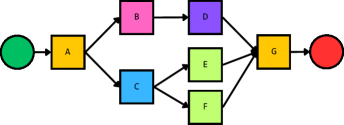
Figure 1: A scientific workflow formed of seven tasks.

Such tasks are typically self-contained programs that are often shared in binary form or as containers. Individual tasks are considered atomic and executed independently on a single machine. To decrease runtime, tasks can be executed on faster machines, and workflows can be executed on clusters in which more resources can be assigned. This enables some tasks to run in parallel when no dependency exists, such as Tasks B and C in Fig. 1. In addition, workflows are often executed on multiple inputs, which allows for data-parallel execution of entire workflows on the allocated cluster resources. Typically, the intermediate results that become inputs of subsequent tasks are exchanged through network file systems, providing flexibility to schedule subsequent tasks on different nodes as well as to recover from persisted intermediate results in case of task failures.

2.2 Carbon Intensity (CI)

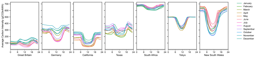
Figure 2: Daily mean average carbon intensity per month in 2024 for the seven regions we studied: Great Britain, Germany, California (USA), Texas (USA), South Africa, Tokyo (Japan), and New South Wales (Australia).

CI measures the carbon emissions produced per unit of electricity consumed. Renewables have lower CI than fossil fuels, but their output levels vary over time. We analyze this fluctuation in seven regions during 2023 in Fig. 2, expanding on a previous analysis in the literature [18].

As CI can be quantified by the average or marginal signal, there has been an ongoing discourse on which signal should be used for carbon-aware optimizations [25]. Average reflects the overall grid emissions, factoring in each energy source’s relative share and emission rate. In contrast, marginal measures the emissions of the specific energy source meeting an additional load. Marginal CI is preferred for measuring the impact of load shifting [23]. However, there are challenges in obtaining the metric owing to computational complexity – marginal CI is only estimated and lacks granularity for accurate reporting. In contrast, average CI can be measured and is often readily available and, therefore, commonly used for reporting. It could also help incentivize investment in renewable energy generation by aligning electricity usage with renewable sources for greater long-term impact [26]. As both signals have advantages and disadvantages, we consider both signals in our exploration of the potential impact of carbon-aware computing methods.

Further, the marginal signal is highly variable and does not follow a predictable pattern in the same way that the average signal often does. In Fig. 3, we plot the average and marginal CI on the 20^th and 27^th of January, 2023. On the same day a week apart, the average CI follows a similar pattern, whereas the marginal CI varies significantly. These dips could indicate windows of time in which electricity has a CI near zero, potentially due to renewable energy being curtailed. Curtailment is the deliberate reduction of electricity generation to balance supply and demand in a grid. It occurs when generation exceeds current grid demand, and the excess power cannot be stored or traded with neighbouring grids.

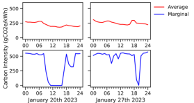
Figure 3: A comparison of average and marginal CI signals for Northern Texas between two days, 20th and 27th of January 2023.

2.3 Operational vs. Embodied Carbon Emissions

Operational carbon refers to emissions generated during the in-use phase of hardware, resulting from the generation of electricity consumed to power computations, data storage, and networking. These emissions are ongoing and directly correlate with the system’s energy efficiency, workload intensity, and the real-time carbon intensity of the electricity grid.

In contrast, embodied carbon emissions are all emissions associated with the manufacturing and lifecycle of the physical hardware. This includes raw material extraction, component fabrication, transportation, assembly, and end-of-life activities such as e-waste processing and disposal. While operational emissions can be mitigated dynamically through strategies like energy-efficient scheduling and carbon-aware load shifting, embodied emissions are a front-loaded carbon investment that is locked in once the hardware is manufactured.

3 Study Design

We capitalize on the fact that scientific workflows are particularly suited to carbon-aware computing, given their delay tolerance, interruptibility, scalability, and heterogeneity. In this paper, we focus on systematically exploring delay tolerance, interruptibility, and scalability leaving the exploitation of heterogeneity for future work. To explore the potential reduction in carbon emissions, we assume perfect knowledge of task and workflow executions – where their execution behaviour aligns with the relevant trace. We also assume that the CI forecasts have no error, making use of historical data. We also assume that we have infinite resource availability when performing time shifting and resource scaling, and do not consider available resource capacity. The identified potential reduction will differ from the actual reduction possible in practice.

For all experiments, we first estimate energy consumption based on resource utilization with linear power models, and then translate this to operational carbon emissions based on commercial-grade average and marginal CI data. We focus on the operational emissions of carbon-aware temporal shifting and resource scaling, but also analyze the impact that optimizations have on embodied emissions.

We describe the experimental setup used in the following evaluation sections. This includes: (1) the selection of real-world Nextflow workflows, (2) the compute resources on which workflows and their tasks were executed, and (3) the CI data for the region where these were executed.

3.1 Scientific Workflows

We study five of the ten most popular real-world bioinformatics workflows from Nextflow’s community-curated nf-core library [27], an astronomy workflow, and another from the Earth observation domain. These are representative of the domains they work with. Table 1 details these workflows.

Table 1: The seven real-world workflows selected for investigation.

Workflow	Domain	# Physical Tasks
Chip-Seq [28]	Bioinformatics	3,536
MAG [29]	Bioinformatics	7,477
Montage [1]	Astronomy	197
Nano-Seq [30]	Bioinformatics	91
Rangeland [8]	Earth Observation	4,417
RNA-Seq [31]	Bioinformatics	1,268
Sarek [32, 33]	Bioinformatics	8,954

To minimize carbon emissions in our study, we rely on existing historical traces wherever possible. Specifically, we used trace files [34] for MAG and Rangeland [35] and for Chip-Seq, Montage, RNA-Seq, and Sarek from [36]. Meanwhile, we ran the Nano-Seq workflow on an edge server, as well as several individual workflow tasks on cloud and cluster resources.

3.2 Compute Resources

In this study, we work with various nodes, which are detailed in Table 2. We used three types of Google Compute Platform (GCP) nodes, all prefixed with “gcp”, and five other types of nodes – some of which are individual edge servers while others like – olympus, atlantis and camelot are part of homogeneous clusters. These resources represent diverse and relevant compute environments for scientific workflow execution. We also document the Life Cycle Assessment (LCA), that is, the associated carbon emissions tied to each compute resource over its lifetime, retrieved from the Boavizta API [37].

Table 2: The compute resources used in the study, and their associated LCA emissions.

		Memory	LCA Emissions
Name	Hardware	(GB)	($kgCO2e$)
gcp-c2	c2-standard-8	32	19.00
gcp-n1	n1-standard-2	7.5	19.00
gcp-n2	n2-highmem-8	32	19.00
atlantis	AMD EPYC 7282	128	23.17
camelot	Intel Xeon Silver 4314	256	21.00
elysium	Intel Xeon Gold 6426Y	128	46.73
olympus	Intel Xeon E5-2640	64	19.80
sherwood	Intel i7-10700T	32	12.37

3.3 Energy Consumption Estimation

In our experiments, we estimate the carbon footprint from executing scientific workflows and their tasks. To achieve this, we used Ichnos [38]. It is a tool built to estimate the carbon footprint of Nextflow workflows from workflow traces, and allows users to provide power models for the compute resources utilized. We utilized Ichnos’s implementation of a linear power model to estimate the energy consumption of resources, translating this to a carbon footprint with fine-grained CI data aligning with each workflow’s execution. Ichnos enables post-hoc energy consumption estimation. When we compared the actual energy consumed, monitored using RAPL, we found that Ichnos’ estimations were more accurate (4–10% error) than other estimation methodologies like CCF  (14–48% error) or GA  (81–98%).

3.4 Carbon Intensity Data

We performed all footprint estimations using average and marginal CI data sourced from Electricity Maps and WattTime. Given that Electricity Maps’ average CI data was offered with hourly intervals, and WattTime’s marginal CI data was offered with 5m intervals, we used the most granular CI data available for associated experiments, i.e., 5m for marginal CI and 60m for average CI.

We selected seven regions, including those where the workflows were originally executed and others where electricity was generated from different renewable sources, prioritizing regions that have a significant data center presence. We selected regions from each continent to increase our representativeness. We selected Great Britain and Germany as they were the regions in which the scientific workflows were originally executed. We selected Texas, as it has led the US in energy generation from wind renewables; California, as it is the highest solar power generating state in the US; along with New South Wales, Tokyo and South Africa, as they, similar to Texas and California, have a significant data center presence as well as variable renewable energy sources.

4 Carbon Footprint Estimation for Workflows

To further motivate our paper’s focus, as well as to establish baselines for the subsequent experiments, we first estimate the operational and embodied carbon emissions generated from the original workflow executions.

We begin by estimating the carbon footprint for the Chip-Seq, MAG, Montage, Nano-Seq, Rangeland, RNA-Seq, and Sarek workflows. These estimations are collated in Table 3. They are based on the mean of three executions of each identified workflow. We present each workflow’s energy consumption on the utilized compute resources. We then translate this into carbon emissions, using either average and marginal CI data, based on the original start and execution times. We estimated the embodied carbon footprint for the execution of each workflow by dividing the workflow’s runtime by the hardware’s expected lifetime (taken as 4 years for CPUs following the CCF methodology ²) and attributing this share to the utilised hardware’s LCA emissions.

Table 3: Operational and embodied (Emb.) carbon emissions (emis) estimated for the selected workflows’ original execution, using average (Avg.) and marginal (Marg.) CI.

		Energy	Avg. emis	Marg. emis	Emb. emis
Workflow	Resources	(kWh)	(gCO2e)	(gCO2e)	(gCO2e)
Chip-Seq	atlantis x8	23.20	12,795.40	18,823.90	117.89
MAG	camelot x8	32.88	6,649.07	23,261.00	213.10
Montage	atlantis x8	0.95	510.29	142.05	5.05
Nano-Seq	sherwood	0.35	30.29	142.05	2.82
Rangeland	camelot x8	11.18	2,724.57	7,901.27	70.23
RNA-Seq	atlantis x8	14.70	3,832.38	11,698.40	74.52
Sarek	atlantis x8	42.45	16,645.90	33,220.40	225.00

Energy consumption varied significantly across workflows executed and resources utilized. However, the carbon emissions produced from each execution also depend on when and in which region workflows were executed. In this paragraph, we focus on estimating the produced carbon emissions using the average CI signal. Nano-Seq was executed in Great Britain, producing emissions of 86.5 $g/kWh$ of energy consumed. Montage was executed in Germany, producing 537.1 $g/kWh$. These rates depend on how carbon-intensive electricity in each region is, e.g., Great Britain being notably lower than Germany. If we compare two different workflows that were executed in Germany on the same compute resources, we see that their emission rate differs significantly. While RNA-Seq produced emissions of 260.7 $g/kWh$, Chip-Seq produced 551.5 $g/kWh$. These rates differ due to the CI fluctuating over time, with both workflows running at different times.

These estimates of carbon emissions account for the energy consumption of all individual workflow tasks. This considers each task’s runtime, CPU utilization over this period, and the memory allocated for each task. However, the compute resources used were assumed to be reserved solely for these workflows, so we can also factor in the whole memory available on each node. We, therefore, estimated the energy consumption for the ‘reserved memory’, which refers to the full memory available on all utilized nodes over the workflow’s execution. These are listed in Table 4. Here, we show the percentage of the overall total (the sum of workflow emissions and reserved memory emissions) that memory accounts for, which is between 5–34% of overall emissions. This percentage of overall emissions depends on the compute resources utilized, the memory available on those resources, and the runtime of the workflow executed. Since workflows can also be executed on shared compute resources, we do not consider full node memory emissions in this way in our evaluation of carbon-aware shifting and scaling in Sections 5– 6.

Table 4: Carbon emissions (emis) produced from reserving node memory over workflow execution, using average CI.

		Energy	Avg. emis	Overall
Workflow	Resources	(kWh)	(gCO2e)	emis (%)
Chip-Seq	atlantis x8	1.49	817.55	6.0
MAG	camelot x8	10.14	2,049.77	23.6
Montage	atlantis x8	0.21	114.31	18.3
Nano-Seq	sherwood	0.07	5.75	16.0
Rangeland	camelot x8	5.53	1,379.30	33.6
RNA-Seq	atlantis x8	1.23	319.14	7.7
Sarek	atlantis x8	2.04	793.84	4.6

It is clear that the carbon emissions produced by scientific workflows are significant. Executing these workflows resulted in up to 17 $\mathrm{kg}$ of carbon emissions for a single run (0.3–78 $\mathrm{kg}$ for three executions). For comparison, 17 $\mathrm{kg}$ of carbon emissions is equivalent to the greenhouse gas emissions produced by driving $\approx$70 $\mathrm{km}$ in an average petrol-powered car.

5 Potential of Carbon-Aware Load Shifting

In this section, we explore how entire workflow applications can be temporally shifted, how workflows can be paused and resumed to further reduce their carbon footprint, and the impact of temporal shifting in seven regions around the world.

5.1 Entire Workflow Shifting

In our first experiment, the start time of an entire workflow’s execution is systematically adjusted by an hour, for every hour within a specified “flexibility window” to measure the potential reduction possible without further adjusting the workflow’s execution.

To ensure that our results were comparable and that we considered the changing seasons of the year, we shifted each workflow’s start time to 9AM on the second Monday of each month in 2024. We then considered two such flexibility windows from this start time: one of 24 hours and the other of 96 hours. This is to mimic the scenario where scientists could delay starting their workflow for up to a day, or over the working week. We explored the possible reduction using average and marginal CI signals, with the full results in A. We performed the experiment for all seven regions, and discuss the impact of the entire workflow shifting in selected regions.

Results Interpretation

In the figures that follow, we present the maximum possible reduction in footprint of each workflow (on the y-axis), for each month of the year (on the x-axis) – this reduction is shown for a 24h window on the left, and a 96h window on the right. The heatmap shows reductions according to the shade of green, with darker shades meaning greater reductions. The percentage reduction is also shown on the heatmap. A reduction of 100% is denoted as “X”.

Average CI

In Fig. 4, we show the reduction possible using the average CI in Great Britain, which has a significant renewables presence. We see that longer shifting windows enable greater carbon reductions, with most workflows responding well to entire workflow shifting.

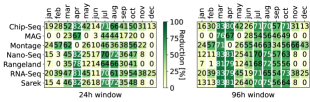
Figure 4: Reduction using entire workflow shifting in Great Britain

However, the reduction potential depended on where and when the original workflows were executed, and the CI levels of the surrounding weekdays. For example, Fig. 5 shows the reduction potential in South Africa, using the average CI signal. Here, we see that there is little to no benefit from entire workflow shifting in either window. The region of South Africa’s has a consistently high CI, with notably lower variability than other regions examined in this study (Fig. 2).

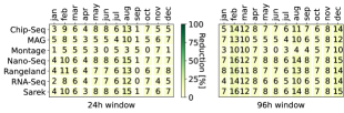
Figure 5: Reduction using entire workflow shifting in South Africa

Marginal CI

When we performed the same experiments with the marginal CI signal, the potential impact of the entire workflow shifting was highlighted further. Given that the marginal signal is likely to indicate periods of time where the grid is curtailing renewable energy generation, or under low demand, we can observe a CI near zero over these periods.

In Fig. 6, we show the reduction possible for California, which has a significant solar renewable generation presence. Here, we see that there is little-to-no reduction in a 24h window; but this increases significantly in a 96h window, most notably in September, where there was a period of low CI. This highlights the potential for reductions with increased flexibility of longer time horizons.

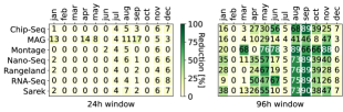
Figure 6: Reduction using Entire Workflow Shifting in California

In Fig. 7, we show the reduction possible for Texas, which has a significant wind renewable generation presence. We similarly observe that increasing the length of the window offers significant benefits for all workflows in several months of the year. In particular, we see that in some months like April, we can reduce the footprint by more than 86%. However, this is reliant on the renewable signal capturing appropriate periods of low-carbon energy, and those periods occurring in a given region.

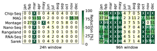
Figure 7: Reduction using entire workflow shifting in Texas

Summary

In this experiment, we observed that the potential reduction in emissions depends on where and when workflows could be executed, as the CI fluctuation is more pronounced in some regions with a greater renewables presence, while others may offer little benefit. Increasing the duration of the flexibility window tends to yield further reductions especially in regions with greater CI fluctuations.

Impact on Embodied Emissions

When we perform entire workflow shifting, we focus on the impact of delaying a workflow’s execution, therefore we do not alter the runtime. Consequently, we observe no changes to the embodied carbon footprint when compared to the baseline executions (refer to Table 3).

5.2 Interrupted Workflow Shifting

In our second experiment, we considered how scientific workflows could be interrupted to exploit multiple shorter periods of low-carbon energy. For this experiment, we reflect that individual tasks cannot generally be paused and resumed, but that their start can be delayed without significant overhead. As workflow systems like Nextflow use disk storage to exchange intermediate results, there will be negligible runtime overhead for reading the inputs of tasks from disks at a later point in time. The overhead of pausing and resuming entire workflow applications, hence, mainly stems from having to align task executions with multiple shorter periods of low-carbon energy availability, so that all tasks executed in a given time period finish fully within the given periods.

Overhead Estimation

As we used hourly granularity for CI data from both Electricity Maps and WattTime, we divided tasks from each entire workflow’s execution into hourly windows as illustrated in Fig. 8. These windows contain two types of tasks: (i) complete tasks that start and finish in the current hour, e.g., task a; and (ii) partial tasks that start in the current hour but finish later, e.g., tasks b and c.

Dividing tasks into hourly windows allows their execution to be aligned with multiple non-consecutive low-carbon windows of the CI time series. However, interrupting workflows introduces overhead, as tasks unable to finish within an hourly window have to be delayed to a later window. As multiple tasks are possibly delayed in this way, we can consider the task that is most delayed, that is, the longest partial task that runs within the window (the purple box around task c), as an upper bound of overhead. The overall overhead is the sum of the overheads of individual windows for every interval where an interruption occurred.

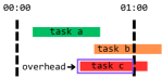
Figure 8: Defining hourly execution windows for workflow tasks and overheads.

We mapped the task execution windows to the lowest carbon intervals in a given flexibility window, in chronological order, to align with the workflow’s original execution and data dependencies. Our results for average and marginal CI explore the potential reduction in carbon emissions for our selected workflows, highlighting the potential for temporal shifting in each original execution environment. In each of our selected regions, we explored the reduction possible by applying temporal shifting with interruptions. The full results are available in B.

Results Interpretation

In each graph, we show the percentage reduction in the carbon footprint, taking the mean reduction for our selected workflows with bar plots (on the y-axis). We calculated this reduction for each month of the year, using the same week as in the entire workflow shifting experiment (Section 5.1). Each bar plot is formed of five blocks, representing the reduction possible in each of five flexibility windows. For example, in Fig. 9, we see that in January, we could save around 20% with the 12-hour window. Increasing the window to 24h, savings are increased to 25%. Increasing the window size further does not yield additional reductions.

Average CI

In Fig. 9, which shows the reduction possible using interrupted shifting in Great Britain, we see that we can reduce the footprint by over 20% in each month of the year, with much greater reductions possible by extending the flexibility window to at least 48h in some months of the year. We also see that the additional benefit in waiting 96h is small, and is only found in some months of the year. While these figures are similar to those from the entire workflow shifting experiment, we can achieve similar savings in a window of just 48h instead of 96h.

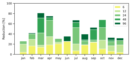
Figure 9: Footprint Reduction using Interrupted Shifting in Great Britain over windows of 6–96h.

In Fig. 10, we show the reduction possible in California. Here, we see that our workflows footprint can be reduced by 40–65% across all months of the year in a flexibility window of just 6–12h. Such underlines the potential of interrupted shifting over a short window, such as waiting from the morning until the evening, or from night to day. In contrast, using entire workflow shifting in the same region offers far lower reduction potential – showing the benefit of interruptions in a region with a significantly variable solar renewable generation.

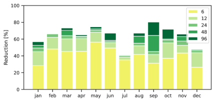
Figure 10: Footprint Reduction using Interrupted Shifting in California over windows of 6–96h.

However, some regions, such as South Africa (see Fig. 11) have relatively steady CI due to being heavily reliant on fossil fuels like coal. In such regions, there is little reduction potential from workflow shifting with and without interruptions.

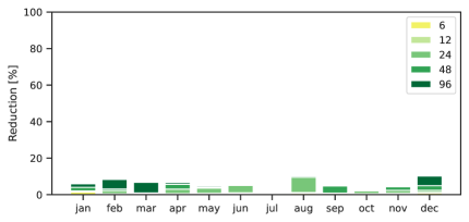
Figure 11: Footprint Reduction using Interrupted Shifting in South Africa over windows of 6–96h.

Given that our implementation of interrupted workflow shifting relies on workflow executions being divided into set execution windows, it may not find the ‘optimal’ schedule for a workflow. However, it implements a form of interrupted workflow shifting that can outperform entire workflow shifting, or achieve savings in a shorter time – highlighting its potential.

Marginal CI

When using the marginal signal, our results from interrupted workflow shifting were much less consistent, given that the signal exhibits less regular patterns in CI fluctuation, leading to shorter windows of low-carbon energy. In Germany, which typically has fluctuating CI (see Fig. 2), we see little reduction in the footprint of our workflows throughout the year. The most potential is observed in May, with a potential reduction of around 45%, due to the presence of low-carbon intensity windows.

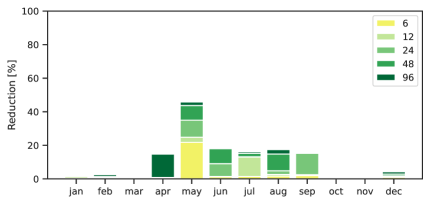
Figure 12: Footprint Reduction using Interrupted Shifting in Germany over windows of 6–96h.

This is different for regions like California, which produces a significant amount of energy from solar. When using the marginal signal, we see potential for the footprint to be significantly reduced in February–June and October of 2024, with reductions of more than 70% in the 96h window. However, in July–September, we note fewer low-carbon windows, potentially caused by the combination of increased energy usage and lower energy curtailment, resulting in a higher CI and less footprint reduction potential.

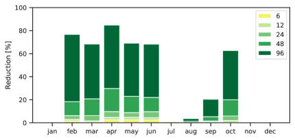
Figure 13: Footprint Reduction using Interrupted Shifting in California over windows of 6–96h.

Summary

Using marginal CI highlights the potential of leveraging a signal that could indicate energy curtailment or low grid demand, enabling scientists to execute workflows with essentially zero operational carbon emissions.

Impact on Embodied Emissions

When we perform interrupted workflow shifting, we introduce time overhead by pausing and resuming execution. This is because the nodes used to run the workflow remain reserved during interruptions, despite being inactive. We observe a resultant increase in embodied carbon emissions of 0.03$g$. However, the mean reduction in average carbon emissions from applying interrupted shifting is 1,612.1$g$. Therefore, the increase in embodied emissions has a negligible impact on the overall carbon footprint.

6 Potential of Resource Scaling

We explored the potential of carbon-aware scaling across two dimensions: (i) Resource selection, the impact of using different devices for individual workflow tasks; and (ii) Frequency scaling, the impact of using different processor governors for individual tasks and entire workflows. We also include an example of adjusting the cluster size for the execution of an entire workflow.

We study the following workflow tasks: bowtie2_build, fastp, fastqc and trimgalore. All four of these tasks are from the twenty most used bioinformatics tasks from Nextflow’s community-curated nf-core library [27].

6.1 Adjusting Compute Resources Used

In our first experiment, we explored the impact of choosing different nodes to execute the individual workflow tasks. We executed each task three times on each resource: three GCP nodes, three olympus nodes, elysium, camelot and sherwood (see Table 2).

To ensure our results were comparable, we adjusted the start time consistently for each task, where bowtie2_build started at 09:00, fastp at 11:00, fastqc at 13:00 and trimgalore at 15:00. Each task was adjusted for the ’median’ day of each month of the year (the day which fell in the middle of the month), in each of our selected regions. Task runtime, energy consumption, and carbon emissions from the mean of three executions on each node are shown in Table 5.

Task	Dimension	Machines
		gcp-c2	gcp-n2	gcp-n1	olympus-1	olympus-2	olympus-3	elysium	camelot	sherwood
	runtime	0.16	0.18	0.25	0.25	0.25	0.25	0.15	0.16	0.14
bowtie2	energy	0.003	0.001	0.001	0.016	0.016	0.017	0.029	0.014	0.004
_build	avg. emis	0.99	0.34	0.38	5.18	5.28	5.67	9.43	4.74	1.33
	marg. emis	0.83	0.33	0.45	6.11	6.25	6.74	7.18	4.03	0.96
	emb. emis	0.09	0.10	0.13	0.13	0.13	0.14	0.19	0.09	0.06
fastp	runtime	0.06	0.08	0.15	0.14	0.16	0.17	0.11	0.05	0.05
	energy	0.001	0.001	0.001	0.009	0.010	0.012	0.022	0.005	0.002
	avg emis	0.49	0.26	0.35	3.03	3.47	3.87	7.24	1.50	0.53
	marg emis	0.87	0.46	0.28	2.33	3.04	3.92	3.41	2.67	0.96
	emb. emis	0.03	0.04	0.08	0.08	0.09	0.09	0.15	0.03	0.02
fastqc	runtime	0.18	0.21	0.26	0.26	0.26	0.26	0.13	0.16	0.16
	energy	0.003	0.001	0.001	0.016	0.017	0.018	0.025	0.015	0.005
	avg emis	1.18	0.41	0.42	5.72	5.87	6.24	8.67	5.13	1.65
	marg emis	1.12	0.44	0.51	6.88	7.03	7.49	5.19	4.41	1.35
	emb. emis	0.10	0.11	0.14	0.14	0.14	0.14	0.17	0.09	0.07
trimgalore	runtime	1.07	1.28	1.93	1.50	1.49	1.56	0.86	1.05	1.0
	energy	0.002	0.002	0.006	0.032	0.032	0.039	0.168	0.087	0.020
	avg emis	0.58	0.75	2.31	11.77	11.62	14.00	59.16	36.93	7.26
	marg emis	12.70	5.17	7.44	53.74	53.97	60.05	92.30	51.44	16.25
	emb. emis	0.58	0.69	1.04	0.81	0.81	0.84	1.14	0.57	0.29

Table 5: Resource Assignment results: each task’s runtime is reported in hours, its energy in $kWh$, and its average (avg.), marginal (marg.), and embodied (emb.) emissions (emis), in $gCO_{2}e$, using CI data for Great Britain. Values in bold represent the minimum runtime, energy and emissions.

Across all nodes, the bowtie2_build task took between 9–15m to run. The execution on elysium had the shortest runtime, but consumed the most energy, 0.029$kWh$. This was almost two times the energy consumed by olympus-1, which took longer but only consumed 0.016$kWh$. The choice of node significantly impacted the runtime of these tasks, with the trimgalore task taking between 52m–1h56m across all nodes.

We note that the GCP machines show comparatively low energy consumption, and separate these results in the table. It is more challenging to accurately estimate energy consumption in the cloud, given that we could not perform power measurements on the nodes to fit power models. Therefore, we were reliant on average energy coefficients used by CCF ², and believe that there is greater potential for discrepancies here.

While the results from the experiment show that the sherwood and gcp-n2 nodes would allow for carbon emissions to be minimised (from each set of devices), changing the device that a task runs on can significantly impact the runtime, energy consumption and carbon emissions. It is important to consider workflow constraints such as scientists’ deadlines or subsequent workflow tasks being dependent on the results produced by tasks to choose particular devices during workflow execution. Additionally, it is possible that task executions could be aligned with low-carbon intervals by selecting appropriate devices.

Impact on Embodied Emissions

Table 5 shows the estimated embodied carbon emissions of each task on each machine. Two factors impact the embodied emissions: the LCA emissions associated with each machine, and the runtime of the task on each machine. For the individual compute nodes, we found that sherwood minimised the embodied carbon emissions for all tasks, given that the node had the lowest LCA emissions and the lowest task runtimes. For the GCP nodes, gcp-c2 had the lowest emissions, given that it had the lowest task runtimes.

6.2 Adjusting Processor Governor Settings

Next, we explored the impact of frequency scaling, by running individual workflow tasks on nodes where the processor governor was changed. We focused on processor governor settings, as scientists might not have the permissions or expertise required to choose a specific frequency, and nodes may operate using pre-selected governors.

A processor’s governor is a component that is used to manage the CPU clock speed in response to changes in system load. We focus on two Intel governors: performance, which forces the CPU to always run at the highest possible frequency; powersave, which forces the CPU to run at the lowest possible frequency. For each selected resource, we took separate power measurements as a basis for estimating energy consumption for each governor setting.

We executed the tasks on three olympus nodes, elysium, camelot and sherwood, as presented in Table 2. For all executions of the selected tasks, we adjusted the start times to the same as that of the resource assignment experiment, again using the median day in each month. In our discussion we use the estimated carbon emissions using CI data for Great Britain.

In Table 6, we compare the nodes elysium and camelot. The elysium node is the most powerful and newest node that we studied, while camelot is several years older. We observed that for elysium, changing the governor from performance to powersave had little impact on the runtime of each task – with the powersave governor consuming slightly less energy, and producing slightly less carbon emissions. In contrast, we observe a far greater difference between governor settings for camelot. The runtime of each task is around four times longer when using the powersave governor. Given the increase in task runtime, using the powersave governor consumes around twice the energy of the performance governor. On this node, we might therefore generally prefer to use the performance governor to reduce our runtime, energy consumption, and carbon emissions. Furthermore, when comparing these nodes, using camelot with the performance governor would offer the minimum energy consumption and carbon emissions, despite not always having the shortest runtime.

		Node elysium		Node camelot
Task	Dimension	Governor		Governor
		perf.	save.	perf.	save.
	runtime	0.15	0.15	0.16	0.64
bowtie2	energy	0.029	0.027	0.014	0.028
_build	avg. emis	2.77	2.59	1.39	2.72
	marg. emis	4.98	4.67	2.79	9.9
	emb. emis	0.16	0.16	0.07	0.28
fastp	runtime	0.11	0.11	0.05	0.20
	energy	0.022	0.021	0.005	0.009
	avg. emis	2.13	2.02	0.44	0.86
	marg. emis	2.29	2.48	1.78	2.0
	emb. emis	0.12	0.12	0.02	0.08
fastqc	runtime	0.13	0.13	0.16	0.63
	energy	0.025	0.023	0.015	0.028
	avg. emis	2.99	2.6	1.77	3.35
	marg. emis	3.37	7.29	2.87	9.75
	emb. emis	0.13	0.14	0.07	0.27
trimgalore	runtime	0.86	0.86	1.05	4.27
	energy	0.168	0.158	0.004	0.145
	avg. emis	18.6	19.28	0.45	14.7
	marg. emis	63.22	62.34	35.04	75.28
	emb. emis	0.92	0.92	0.02	1.42

Table 6: Frequency Scaling for elysium and camelot using the performance (perf.) and powersave (save.) governors: each task’s runtime is reported in hours, its energy in $kWh$, its average (avg.), marginal (marg.), and embodied (emb.) emissions in $gCO_{2}e$ using CI data from Great Britain. Values in bold represent the minimum runtime, energy and emissions.

However, the task-level experiment did not consider the impact of frequency scaling on an entire workflow. So, our next experiment considered the execution of full workflows, Chip-Seq and RNA-Seq, exploring the impact of the same governors on overall energy consumption and carbon emissions. The results are shown in Table 7. We used the average CI for all selected regions to consider the impact across the world.

Both workflows were executed on a cluster of eight camelot nodes. The Chip-Seq workflow took around 3h18m to execute using the performance governor, consuming 15.3$kWh$ of energy, and around 8h30m to execute using the powersave governor, consuming 21.9$kWh$ of energy. Meanwhile, the RNA-Seq workflow took around 2h24m to execute using the performance governor, consuming 8.5$kWh$ of energy, and around 7h30m to execute on the powersave governor, consuming 11.2$kWh$ of energy. We observe that using the powersave governor results in runtimes of around 2.5–3x the duration of the performance governor when these workflows are executed on this cluster. However, the energy consumption is only around 1.3x higher using the powersave governor. While consuming more overall energy leads to greater carbon emissions using the average CI signal in most of our regions, we notice that in California, we would produce slightly less emissions (2.9$kg$ instead of 3.1$kg$) by using the powersave governor. Therefore, the processor’s governor setting could be adjusted to control the energy consumption over time, to reduce overall emissions.

			Regions
			Great				South		New South
Workflow	Governor	Energy	Britain	Germany	California	Texas	Africa	Tokyo	Wales
Chip-Seq	perf.	15.33	780.68	3484.25	3079.97	4839.22	10012.64	6421.12	8867.67
	save.	21.89	2313.26	4582.53	2909.21	7572.87	14300.91	10365.23	12017.58
RNA-Seq	perf.	8.46	331.42	1438.31	666.72	2273.10	5570.98	4137.80	5347.54
	save.	11.20	687.63	2223.62	1119.74	3753.44	7468.06	4845.66	6163.67

Table 7: Frequency Scaling for Chip-Seq and RNA-Seq workflows using the performance (perf.) and powersave (save.) governors in all regions using average. Values in bold represent the minimum emissions for each workflow in each region.

Impact on Embodied Emissions

Table 6 shows the estimated embodied carbon emissions of each task running with the performance and powersave governors on each machine. We observe that changing the governor impacts the runtime of each task, impacting the embodied emissions. We observed that using camelot with the performance governor resulted in the lowest embodied carbon emissions for all tasks due to the machine’s lower LCA emissions, despite having longer task runtimes.

For entire workflow execution, we observed that using the performance governor resulted in lower embodied carbon emissions than the powersave governor, as it reduced the workflow’s runtime.

6.3 Adjusting Cluster Size for Entire Workflow Execution

We additionally used workflow traces to explore the execution of the Chip-Seq workflow on a cluster formed of 2, 4 and 8 atlantis nodes using CI data for Germany during October to December 2023.

Table 8: Carbon Emissions (emis) for Chip-Seq on different cluster sizes. Values in bold represent the minimum runtime, energy and emissions.

#	Runtime	Energy	Avg. emis	Marg. emis	Emb. emis
Nodes	(h)	(kWh)	(gCO2e)	(gCO2e)	(gCO2e)
2	11.84	34.13	11,862.16	25,387.30	15.65
4	5.97	34.39	9,616.61	25,968.88	15.78
8	3.13	34.17	6,817.35	23,639.88	16.55

As shown in Table 8, executing the workflow consumed the same amount of energy at different scales, yet the runtime reduced as the number of nodes increased. We see that the execution on two nodes took 12 hours, while the execution on eight nodes took only 3 hours. These decreases in runtime lead to a reduction in the carbon footprint due to the given CI data. However, further reductions could be made by aligning shorter executions optimally with low-carbon windows of electricity.

Impact on Embodied Emissions

In this case, the total LCA emissions scale with the number of nodes utilised. However, since the runtime reduction will never perfectly scale with additional nodes, we expect the embodied emissions to increase slightly. This is reflected in Table 8.

7 Discussion

In this section, we discuss the key takeaways from our experiments and threats to the validity of our evaluation.

7.1 Key Takeaways

Carbon-Aware Workflow Shifting

In Section 5.1, we shifted the execution of entire workflows within a flexibility window to assess the potential reduction in carbon emissions. As the length of this flexibility window was increased, the potential reduction in carbon emissions also increased. This demonstrates that the delay tolerance of many scientific workflows can be leveraged for low-carbon execution. While temporal shifting achieved carbon emission reductions in most of our selected regions, some regions, such as South Africa, exhibited minimal reductions due to their lower renewable energy generation and, accordingly, fewer fluctuations in the energy mix compared to regions like Great Britain.

Finding 1.

In regions with a significant presence of renewable energy sources and fluctuating CI, temporal shifting of entire workflows could result in carbon footprint reductions of over 80% using average CI.

Interruptible Workload Shifting

In Section 5.2, we went beyond shifting entire workflows by dividing execution into execution windows that could be mapped to multiple lowest-carbon CI intervals. These experiments found that interrupted workflow shifting could achieve greater savings in carbon emissions in a shorter time than entire workflow shifting. In particular, California showed the potential for reductions of 30–70% in a flexibility window of 6–24h, and up to 80% in a window of 96h, throughout the year. This significantly improves over the reductions possible for California when shifting entire workflows.

Moreover, our experiments with Marginal CI highlighted that the choice of signal used when shifting is important, and impacts potential reductions. The marginal signal could indicate periods of time where energy is curtailed, or the grid has low demand, to execute workflows with little-to-no operational emissions.

Finding 2.

Shifting workflows with interruptions can amplify savings, e.g., 30–70% in a 24h window, improving from reductions of $<$20% using entire workflow shifting in the same window for all workflows within regions that have a significant presence of renewable energy, using average CI.

Carbon-Aware Resource Scaling

In Section 6, we demonstrated how choosing different nodes impacted the runtime, energy consumption and carbon emissions of four tasks. We found that the choice of device significantly changed these properties of tasks. If we wanted to execute a workflow in a carbon-aware manner, we could choose to run tasks on specific devices to closely align with low-carbon windows. Next, we explored the impact of frequency scaling, comparing the powersave and performance governors at an individual task and entire workflow granularity. Here, we saw that each governor offered different benefits. Powersave tended to take longer but consumed less energy over the same period of time, while performance led to more work being completed in a shorter time, but consumed more energy to achieve this goal. Alternating between these governors could lead to a workflow’s energy consumption being adjusted depending on the region’s CI. We also showed that adjusting the cluster size for the Chip-Seq workflow could significantly impact runtime to highlight the potential for carbon-aware resource scaling for entire workflows. For example, more computing resources could be allocated to low-carbon windows to reduce the workflow footprint. Such methods could be combined with carbon-aware interruptible shifting to divide workloads into groups of tasks that maintain workflow data dependencies, while making the best use of forecasted low-carbon windows.

Finding 3.

Resource scaling can shape runtimes of workflows and their tasks to fit upcoming low-carbon energy availability, e.g., if Chip-Seq used the performance governor instead of powersave, it could reduce carbon emissions by 67% on the same compute cluster.

7.2 Threats to Validity

Power Estimation vs. Measurement

To estimate the carbon footprint of workflow and task execution, we used readily available Nextflow trace files to avoid unnecessary emissions. Consequently, we could only estimate energy consumption using a linear power model, which is less accurate than directly monitoring energy consumption of compute resources with hardware or software power meters [39, 38]. However, consistently using the same methodology for baseline footprint estimates and footprints from applying carbon-aware computing methods should result in representative relative values reporting the potential footprint reduction. Moreover, widely used footprint assessment methodologies, such as CCF² and Green Algorithms³ also rely on linear power models.

Temporal Shifting and Scaling Assumptions

We estimated the footprint for all possible time-shifting scenarios within a given flexibility window with and without interruptions. This approach is based on unrealistic knowledge of workflow runtimes, resource availability, and error-free CI forecasts. These assumptions represent idealised conditions that do not necessarily reflect real-world conditions.

However, many schedulers are reliant on such signals [40, 13, 41], and existing methods used to predict the runtime and energy consumption of workflow tasks can have a low error [42, 43, 44]. Meanwhile, CI forecast services like ElectricityMaps (reports a 10–15% error) and WattTime (reports a 1–9% error) are widely used.

We also made the assumption that we had unlimited capacity and resource availability when time-shifting, or choosing between devices or scaling a compute cluster in our resource scaling experiments.

Nevertheless, we emphasize that our study explored the potential emissions reduction, providing an upper bound on the possible gains, but not how this potential can be achieved in practice. We maintain that these results help us by quantifying the maximum environmental impact of carbon-aware computing techniques for scientific workflow execution.

Coverage of Renewable Energy Signals

In our experiments, we estimated the carbon footprint using hourly average and marginal CI data. This aligns with most carbon-aware computing research that uses these signals presented in Section 8. Future work could consider more granular data – in line with available CI forecasting, as the most granular historical data were only available at an hourly level. While other metrics for renewable energy accounting exist (e.g., market-based measures such as RECs and PPAs), we did not focus on these as they do not necessarily reflect low-carbon energy availability at a certain time and place.

Workflow System Representativeness

While this study only focuses on a single SWMS (Nextflow), the workflow properties we highlight (delay tolerance, interruptibility, scalability, and heterogeneity) are common across many SWMSs. Therefore, the potential reduction in emissions from applying carbon-aware methods should apply to using other SWMS as well.

Scale of Footprint Reduction

Our evaluation demonstrates the potential for substantial emission savings, e.g., kilograms of carbon emissions for medium-scale workflows that run for up to 12h. While these workflows may have a smaller individual footprint than those running for thousands of core hours (e.g.,  [7]), they are frequently executed by scientists. We expect the potential emission savings identified for medium-scale workflows to scale proportionally to larger computational tasks, given also larger infrastructures and larger flexibility windows.

8 Related Work

Temporal Shifting

Various works propose to schedule or interrupt applications to only consume electricity when CI is low. Through simulations, Wiesner et al. [18] explored delaying or interrupting flexible workloads, such as ML training, to reduce carbon emissions. Google’s Carbon-Intelligent Compute Management [21] uses average CI forecasts to set capacity limits for data centers, thereby delaying flexible workloads. Lin et al. [45] create capacity plans for hyperscale data centers using day-ahead forecasting, and share these plans with the grid to avoid grid instability.

Other studies aim to only leverage excess renewable energy. Zheng et al. [46] discuss the potential for load to be migrated between data centers to make use of energy that would otherwise be curtailed. Cucumber [47] is a configurable admission control policy to execute delay-tolerant workloads in edge data centers equipped with on-site renewable energy sources. Similarly, FedZero [48] schedules Federated Learning exclusively on renewable excess energy and spare compute capacity. None of these works specifically optimizes workflow applications.

Resource Scaling

Carbon-aware resource scaling dynamically allocates more resources when CI is low and reduces demand when it is higher. CarbonScaler [20] performs horizontal scaling based on one-time offline profiling, executing the job for a short period to determine a scaling factor. As such, this factor may not accurately reflect the later stages of a distributed job, such as the various tasks of larger workflows.

Carbon Containers [22] proposes a system-level method that combines vertical scaling, container migration, and temporal shifting to control and limit the carbon emissions rate of containerized applications. The approach focuses on individual containers and is not directly applicable to multi-stage applications like scientific workflows.

Other Carbon-Aware Computing Techniques

Other work has yielded carbon-aware computing techniques and tools to prioritize sustainability. Carbon Explorer [49] is a tool to predict carbon-optimal strategies for operating data centers, considering renewable energy investment, energy storage, and carbon-aware shifting. Chien et al. [50] studied the impact of carbon-aware algorithms on emissions generated by generative AI through shifting requests to locations with low-carbon power. Ecovisor [19] virtualizes the energy system to allow applications to control how they use renewable energy, relying on application developers to manage carbon emissions at runtime. Wen et al. [51] propose an algorithm to increase the usage of green energy when executing industrial workflows, but they only evaluate the impact of location-based load shifting, assigning data centers a static measure for how ‘green’ the energy mix is, without considering the dynamic nature of renewable energy generation. Lotaru [52] is a method for predicting the runtime of scientific workflows using microbenchmarks that has been shown to be useful for simple carbon-aware time shifting [44]. Crucially, none of these techniques specifically exploits the characteristics of workflows for carbon-aware execution. Schweisgut et al. [53] propose scheduling algorithms to decrease the carbon footprint of scientific workflows by aligning their execution with low-carbon energy. They simulate their algorithms and compare against other scheduling approaches, considering the impact on carbon emissions and workflow runtime. Their work focuses on the carbon-aware scheduling, and does not consider carbon-aware interrupted shifting or resource scaling. In our previous work [24], we highlighted that scientific workflows are typically delay tolerant, interruptible, scalable and heterogeneous, increasing their aptitude for carbon-aware execution. We significantly build on our preliminary results in this study, extending our previous experiments and conduct new ones considering more workflows, tasks and regions.

9 Conclusion

In this paper, we have systematically explored the potential of carbon-aware execution for scientific workflows. To begin with, we estimated the carbon footprint from running seven real-world workflows; they produced up to 17$kg$ of operational carbon emissions. Using these estimates as baselines, we first assessed carbon-aware time shifting, finding that this could reduce the footprint by over 80% using the average CI, and in some scenarios, completely using the marginal CI. We found that interrupted shifting could amplify savings, potentially outperforming entire workflow shifting over the same flexibility windows. We also evaluated resource assignment and frequency scaling, finding that selecting appropriate devices to run workflow tasks could align their execution with low-carbon windows. We also saw that choosing between available processor governors could reduce the footprint of workflow execution by 67%, using the average CI. Based on these results, we discussed how three specific properties of scientific workflows – their delay tolerance, interruptibility, and scalability – could be exploited when applying carbon-aware computing methods.

However, our evaluation of the potential of carbon-aware execution assumed that we had perfect knowledge of task and workflow executions, perfect CI forecasts and infinite resource availability. As such, our evaluation did not consider how this carbon footprint reduction can be achieved in practice. Future work will explore how real-world profiling techniques can be used to measure and predict the performance of workflows, focusing on their runtime, energy consumption and expected carbon footprint on heterogeneous infrastructure. We would then explore how workflow profiles could be combined with CI forecasting and resource availability data to execute workflows in a carbon-aware manner, in practice.

Appendix A Entire Workflow Shifting for all regions

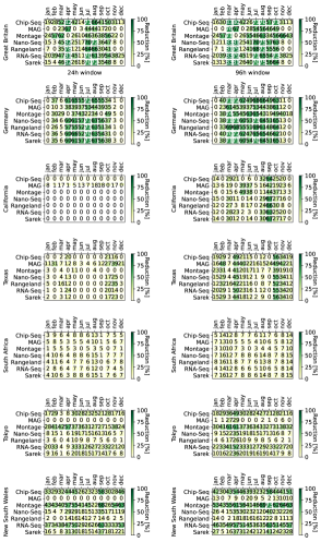
Figure 14: Entire Workflow Shifting – Reduction using Average CI.

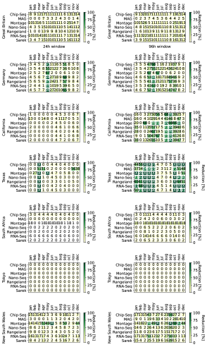
Figure 15: Entire Workflow Shifting – Reduction using Marginal CI.

Appendix B Interrupted Workflow Shifting for all regions

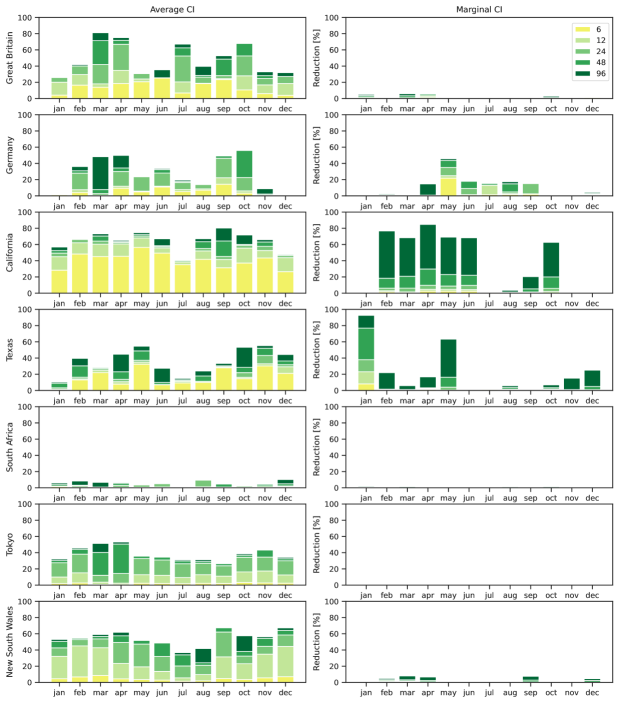
Figure 16: Interrupted Workflow Shifting – Reduction over 12–96h windows using average and marginal CI.

References

- [1] B. Berriman, E. Deelman, J. Good, J. Jacob, D. Katz, C. Kesselman, A. Laity, T. Prince, G. Singh, M.-H. Su, Montage: A grid enabled engine for delivering custom science-grade mosaics on demand, in: Optimizing Scientific Return for Astronomy through Information Technologies, Vol. 5493, SPIE, 2004, pp. 221–232.
- [2] J. A. Fellows Yates, T. C. Lamnidis, M. Borry, A. Andrades Valtueña, Z. Fagernäs, S. Clayton, M. U. Garcia, J. Neukamm, A. Peltzer, Reproducible, portable, and efficient ancient genome reconstruction with nf-core/eager, PeerJ 9.
- [3] J. Schaarschmidt, J. Yuan, T. Strunk, I. Kondov, S. Huber, G. Pizzi, L. Kahle, F. Bölle, I. Castelli, T. Vegge, F. Hanke, T. Hickel, J. Neugebauer, C. Rêgo, W. Wenzel, Workflow Engineering in Materials Design within the BATTERY 2030 + Project, Advanced Energy Materials 12.
- [4] B. Ludäscher, S. Bowers, T. McPhillips, Scientific workflows, in: Ling. Liu, M. T. Özsu (Eds.), Encyclopedia of Database Systems, Springer, 2009.
- [5] P. Di Tommaso, M. Chatzou, E. W. Floden, P. P. Barja, E. Palumbo, C. Notredame, Nextflow enables reproducible computational workflows, Nat. Biotechnol. 35 (4).
- [6] J. Dias, G. Guerra, F. Rochinha, A. L. G. A. Coutinho, P. Valduriez, M. Mattoso, Data-centric iteration in dynamic workflows, Future Gener. Comput. Syst. 46.
- [7] E. Deelman, K. Vahi, M. Rynge, G. Juve, R. Mayani, R. F. da Silva, Pegasus in the Cloud: Science Automation through Workflow Technologies, IEEE Internet Computing 20 (1).
- [8] F. Lehmann, D. Frantz, S. Becker, U. Leser, P. Hostert, Force on nextflow: Scalable analysis of earth observation data on commodity clusters., in: CIKM Workshops, 2021.
- [9] A. Choudhary, M. C. Govil, G. Singh, L. K. Awasthi, E. S. Pilli, Energy-aware scientific workflow scheduling in cloud environment, Cluster Computing 25 (6).
- [10] L. Zhang, L. Wang, Z. Wen, M. Xiao, J. Man, Minimizing energy consumption scheduling algorithm of workflows with cost budget constraint on heterogeneous cloud computing systems, IEEE Access 8.
- [11] P. V. Reddy, K. G. Reddy, A multi-objective based scheduling framework for effective resource utilization in cloud computing, IEEE Access 11.
- [12] Q. Zhu, J. Zhu, G. Agrawal, Power-aware consolidation of scientific workflows in virtualized environments, in: SuperComputing, 2010.
- [13] J. J. Durillo, V. Nae, R. Prodan, Multi-objective energy-efficient workflow scheduling using list-based heuristics, Future Gener. Comput. Syst. 36.
- [14] I. T. Cotes-Ruiz, R. P. Prado, S. García-Galán, J. E. Muñoz-Expósito, N. Ruiz-Reyes, Dynamic voltage frequency scaling simulator for real workflows energy-aware management in green cloud computing, PloS one 12 (1).
- [15] M. Safari, R. Khorsand, Energy-aware scheduling algorithm for time-constrained workflow tasks in DVFS-enabled cloud environment, Simulation Modelling Practice and Theory 87.
- [16] E. Cao, S. Musa, M. Chen, T. Wei, X. Wei, X. Fu, M. Qiu, Energy and reliability-aware task scheduling for cost optimization of DVFS-enabled cloud workflows, IEEE Transactions on Cloud Computing 11 (2).
- [17] A. Prieto, B. Prieto, J. J. Escobar, T. Lampert, Evolution of computing energy efficiency: Koomey’s law revisited, Cluster Computing 28 (1).
- [18] P. Wiesner, I. Behnke, D. Scheinert, K. Gontarska, L. Thamsen, Let’s wait awhile: How temporal workload shifting can reduce carbon emissions in the cloud, in: Middleware, 2021.
- [19] A. Souza, N. Bashir, J. Murillo, W. Hanafy, Q. Liang, D. Irwin, P. Shenoy, Ecovisor: A virtual energy system for carbon-efficient applications, in: ASPLOS, 2023.
- [20] W. A. Hanafy, Q. Liang, N. Bashir, D. Irwin, P. Shenoy, Carbonscaler: Leveraging cloud workload elasticity for optimizing carbon-efficiency, Proc. ACM Meas. Anal. Comput. Syst. 7 (3).
- [21] A. Radovanović, R. Koningstein, I. Schneider, B. Chen, A. Duarte, B. Roy, D. Xiao, M. Haridasan, P. Hung, N. Care, S. Talukdar, E. Mullen, K. Smith, M. Cottman, W. Cirne, Carbon-aware computing for datacenters, IEEE Trans. on Power Systems 38 (2).
- [22] J. Thiede, N. Bashir, D. Irwin, P. Shenoy, Carbon containers: A system-level facility for managing application-level carbon emissions, in: SoCC, 2023.
- [23] H. He, A. Rudkevich, X. Li, R. Tabors, A. Derenchuk, P. Centolella, N. Kumthekar, C. Ling, I. Shavel, Using marginal emission rates to optimize investment in carbon dioxide displacement technologies, The Electricity Journal 34 (9).
- [24] K. West, F. Lehmann, V. Bountris, U. Leser, Y. Elkhatib, L. Thamsen, Exploring the potential of carbon-aware execution for scientific workflows, in: 2025 IEEE 25th International Symposium on Cluster, Cloud and Internet Computing (CCGrid), 2025.
- [25] T. Sukprasert, N. Bashir, A. Souza, D. Irwin, P. Shenoy, On the implications of choosing average versus marginal carbon intensity signals on carbon-aware optimizations, in: e-Energy, 2024.
- [26] N. A. Ryan, J. X. Johnson, G. A. Keoleian, Comparative assessment of models and methods to calculate grid electricity emissions, Environmental science & technology 50 (17).
- [27] P. A. Ewels, A. Peltzer, S. Fillinger, H. Patel, J. Alneberg, A. Wilm, M. U. Garcia, P. Di Tommaso, S. Nahnsen, The nf-core framework for community-curated bioinformatics pipelines, Nat. Biotechnol. 38 (3).
- [28] H. Patel, et al., nf-core/chipseq v2.1.0 - platinum willow sparrow (2024). doi:10.5281/zenodo.3240506.
- [29] S. Krakau, D. Straub, H. Gourlé, G. Gabernet, S. Nahnsen, nf-core/mag: a best-practice pipeline for metagenome hybrid assembly and binning, NAR Genomics and Bioinformatics 4 (1). doi:10.1093/nargab/lqac007.
- [30] H. Patel, et al., nf-core/nanoseq v3.1.0 - nobelium guppy (2023). doi:10.5281/zenodo.3697959.
- [31] H. Patel, et al., nf-core/rnaseq v3.17.0 - neon newt (2024). doi:10.5281/zenodo.1400710.
- [32] F. Hanssen, M. U. Garcia, L. Folkersen, A. Pedersen, F. Lescai, S. Jodoin, E. Miller, M. Seybold, O. Wacker, N. Smith, G. Gabernet, S. Nahnsen, Scalable and efficient DNA sequencing analysis on different compute infrastructures aiding variant discovery, NAR Genomics and Bioinformatics 6 (2).
- [33] M. Garcia, S. Juhos, M. Larsson, P. Olason, M. Martin, J. Eisfeldt, S. DiLorenzo, J. Sandgren, T. Díaz De Ståhl, P. Ewels, V. Wirta, M. Nistér, M. Käller, B. Nystedt, Sarek: A portable workflow for whole-genome sequencing analysis of germline and somatic variants, F1000Research 9 (63).
- [34] F. Lehmann, WOW with Nextflow and Kubernetes – traces and evaluation (Feb. 2025). doi:10.5281/zenodo.14894648.
- [35] F. Lehmann, J. Bader, N. De Mecquenem, X. Wang, V. Bountris, F. Friederici, U. Leser, L. Thamsen, Ponder: Online prediction of task memory requirements for scientific workflows, in: e-Science, 2024.
- [36] F. Lehmann, J. Bader, F. Tschirpke, N. De Mecquenem, A. Lößer, S. Becker, K. Ewa Lewińska, L. Thamsen, U. Leser, WOW: Workflow-Aware Data Movement and Task Scheduling for Dynamic Scientific Workflows, in: IEEE 25th International Symposium on Cluster, Cloud and Internet Computing (CCGrid), Tromsø, Norway, 2025.
- [37] T. Simon, D. Ekchajzer, A. Berthelot, E. Fourboul, S. Rince, R. Rouvoy, Boaviztapi: A bottom-up model to assess the environmental impacts of cloud services, SIGENERGY Energy Inform. Rev. 4 (5).
- [38] K. West, M. Reid, Y. Elkhatib, L. Thamsen, Ichnos: A carbon footprint estimator for scientific workflows, in: LOCO Workshop, 2025.
- [39] M. Jay, V. Ostapenco, L. Lefevre, D. Trystram, A.-C. Orgerie, B. Fichel, An experimental comparison of software-based power meters: focus on cpu and gpu, in: CCGrid, 2023.
- [40] H. Topcuoglu, S. Hariri, M.-Y. Wu, Performance-effective and low-complexity task scheduling for heterogeneous computing, Trans. on Par. and Dist. Sys. 13 (3).
- [41] V. Arabnejad, K. Bubendorfer, B. Ng, Budget and deadline aware e-science workflow scheduling in clouds, IEEE Transactions on Parallel and Distributed Systems 30 (1).
- [42] M. H. Hilman, M. A. Rodriguez, R. Buyya, Task Runtime Prediction in Scientific Workflows Using an Online Incremental Learning Approach, in: UCC, 2018.
- [43] D. Huang, L. Costero, A. Pahlevan, M. Zapater, D. Atienza, CloudProphet: A Machine Learning-Based Performance Prediction for Public Clouds, IEEE Trans. on Sust. Computing 9 (4).
- [44] J. Bader, F. Lehmann, L. Thamsen, U. Leser, O. Kao, Lotaru: Locally predicting workflow task runtimes for resource management on heterogeneous infrastructures, Future Gener. Comput. Syst. 150.
- [45] L. Lin, A. A. Chien, Adapting datacenter capacity for greener datacenters and grid, in: e-Energy, 2023.
- [46] J. Zheng, A. A. Chien, S. Suh, Mitigating curtailment and carbon emissions through load migration between data centers, Joule 4 (10).
- [47] P. Wiesner, D. Scheinert, T. Wittkopp, L. Thamsen, O. Kao, Cucumber: Renewable-aware admission control for delay-tolerant cloud and edge workloads, in: Euro-Par, 2022.
- [48] P. Wiesner, R. Khalili, D. Grinwald, P. Agrawal, L. Thamsen, O. Kao, Fedzero: Leveraging renewable excess energy in federated learning, in: e-Energy, 2024.
- [49] B. Acun, B. Lee, F. Kazhamiaka, K. Maeng, U. Gupta, M. Chakkaravarthy, D. Brooks, C.-J. Wu, Carbon explorer: A holistic framework for designing carbon aware datacenters, in: ASPLOS, 2023.
- [50] A. A. Chien, L. Lin, H. Nguyen, V. Rao, T. Sharma, R. Wijayawardana, Reducing the carbon impact of generative AI inference, in: HotCarbon, 2023.
- [51] Z. Wen, S. Garg, G. S. Aujla, K. Alwasel, D. Puthal, S. Dustdar, A. Y. Zomaya, R. Ranjan, Running industrial workflow applications in a software-defined multicloud environment using green energy aware scheduling algorithm, IEEE Trans. on Industrial Informatics 17 (8).
- [52] J. Bader, F. Lehmann, L. Thamsen, J. Will, U. Leser, O. Kao, Lotaru: Locally estimating runtimes of scientific workflow tasks in heterogeneous clusters, in: SSDBM, 2022.
- [53] D. Schweisgut, A. Benoit, Y. Robert, H. Meyerhenke, Carbon-aware workflow scheduling with fixed mapping and deadline constraint, arXiv preprint arXiv:2507.08725.