Entanglement-enabled imaging through complex media

Abstract

Scattering in complex media scrambles light, obscuring images and hindering applications ranging from astronomy to microscopy. While computational algorithms and wavefront shaping can, in principle, reverse this mixing by exploiting the near-linear nature of light propagation, in practice the inversion process is highly susceptible to limitations such as the finite number of controllable modes, noise, losses, and inaccuracies in the forward model. Consequently, these approaches are only effective under tightly controlled conditions, limiting their impact on real-world imaging. Here, we present a quantum entanglement-based approach that transmits images through complex media without inverting the scattering process. This method exploits a fundamental property of quantum entanglement: the preservation of photon correlations across multiple measurement bases. By tailoring the optical disorder induced by a scattering layer to access one such basis, entanglement-encoded images of arbitrary objects hidden behind the medium can be reconstructed via coincidence detection at the output. In contrast, classical imaging under identical conditions fails, producing only speckle patterns with no object information. Our work introduces a fundamentally new approach to imaging through complex media by leveraging the unique properties of quantum entanglement beyond simple optical correlations. This opens up new avenues for quantum-enhanced imaging and communication in challenging environments.

Transmitting optical spatial information, such as the image of an object, with high fidelity is crucial for numerous applications in optics. Yet, it becomes highly challenging when light propagates through complex disordered media, such as biological tissues, turbulent atmosphere, or multimode fibers, where spatial information is scrambled and the image becomes unreadable [1, 2, 3]. In recent years, efforts to overcome scattering and enable imaging through complex media have led to the development of many techniques [4].

Among these, wavefront shaping has emerged as a powerful tool [5, 6]. In this context, spatial light modulators (SLMs) can be used, for example, to focus light through a complex medium by shaping its wavefront at the input [7]. In non-invasive scenarios, where access to the far side or inside of the medium is not possible, the wavefront correction applied via the SLM can be retrieved for example by optimizing guide stars [7, 8, 9], image quality metrics [10, 11, 12, 13], or via medium modeling [14]. Once the correction is known, wide-field imaging becomes possible within a limited field of view (FOV), allowing light to be steered through the medium to form an image as if it were transparent. This FOV is limited by the medium’s memory effect [15], but can be extended via multiple measurements [16, 17] and multi-plane wavefront correction [18].

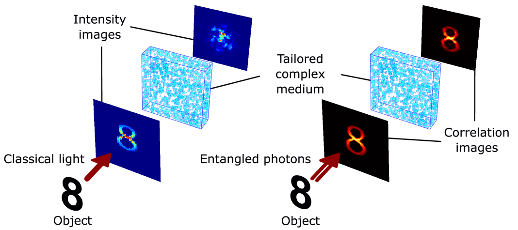
Figure 1: Rendering a complex medium transparent to entangled photons while remaining opaque to classical light. Two imaging scenarios through a complex medium are shown. On the left, an object encoded in classical light intensity is scattered, producing a speckle pattern at the output. On the right, the object is encoded in the spatial correlations of entangled photon pairs. Despite propagation through the same medium, the measured correlation image reveals the object as if the medium were transparent. This is achieved by tailoring the optical disorder of the medium for implementing a specific basis transformation that preserves quantum correlations and thus the encoded image. Both intensity and correlation images are from numerical simulations detailed in Methods and Supplementary Section IV.

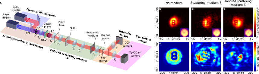
Figure 2: Experimental setup and results. a, A continuous-wave laser at 405nm illuminates an object placed in the object plane of a lens $f_{0}$. The beam is then focused onto a 0.5mm-thick nonlinear $\beta$-barium borate (BBO) crystal, where type-I spontaneous parametric down conversion (SPDC) generates degenerate spatially entangled photon pairs at 810nm. A long-pass filter (LPF) removes the residual pump beam after the crystal. The photon pairs are Fourier-imaged by another lens $f_{1}$ onto the input plane, which is conjugate to the object plane. Before the object, a dichroic mirror (DM) combines the paths of a superluminescent diode (SLED) and the pump laser. The lasers are switched on or off depending on whether the system operates under quantum or classical illumination. Two confocal telescopes formed by the lenses $f_{2}$–$f_{5}$ link the input plane to the output plane. A spatial light modulator (SLM) and a scattering medium (a layer of Parafilm) are positioned in the Fourier planes of the telescopes. The optical transformation $S^{\prime}$ linking the input plane to the output plane is tailored by programming phase patterns onto the SLM. Lenses $f_{i}$ and $f_{c}$, along with movable mirrors, represent two separate imaging systems with magnification $1$, mapping the output plane onto a Charge-Coupled Device (CCD) camera and a time-stamping Tpx3Cam, respectively. A bandpass filter at $810\pm 5$nm (not shown) is used to suppress stray light on both cameras. In the quantum case, correlation images of an entanglement-encoded object (the digit ‘8’) are measured (b) without the scattering medium, (c) after propagation through it, and (d) after tailoring the medium via wavefront shaping. The corresponding intensity images, shown in the insets, reveal no information about the object. In the classical case, intensity images are recorded (e) without the scattering medium, (f) after propagation through it, and (g) after tailoring it. The same scattering medium and tailoring function (i.e. the same SLM phase pattern) are used in both quantum and classical configurations. Correlations images required $8$-second acquisitions, while classical intensity images were acquired withing a few tens of milliseconds. Each image is normalized to its maximum value. See Supplementary Section I for more details about the experimental setup.

Alternatively, computational imaging methods can bypass physical correction performed by an SLM. If part of the scattering matrix of the medium is known [19], it is then possible to reconstruct an object hidden behind the medium from a measured output field or intensity using linear inverse problem algorithms [20, 21]. Even without knowing the matrix, its intrinsic correlations can be exploited to reconstruct an object. For example, provided the object lies within the memory effect range of the medium, direct reconstruction from speckle patterns is achievable using phase retrieval algorithms [22, 23] and bispectrum analysis [24]. Under similar experimental conditions, machine learning approaches have also been used to retrieve hidden objects from speckle image datasets [25, 26, 27].

Despite their diversity, all these techniques share a common principle: restoring imaging by inverting the scattering process. Computational approaches estimate the inverse of the scattering matrix to reconstruct the input field, while wavefront shaping methods physically implement this inverse. Both are based on the same fundamental physics - linear wave propagation in complex media - which is valid in nearly all practical situations and described by a unified framework [19]:

$$E^{\text{out}}=SE^{\text{in}},$$ (1)

where $E^{\text{in}}$ and $E^{\text{out}}$ are vectors representing the input and output fields, and $S$ is the scattering matrix encompassing both the complex medium and the imaging optics.

Paradoxically, the simplicity of Equation (1) is also its main limitation, as it inherently constrains all resolution strategies to the fundamental challenges of linear inverse problems, such as incomplete measurements and sensitivity to noise and losses. Although some approaches incorporate nonlinear effects [28, 29, 30], these are typically used only to aid convergence towards a solution of Equation (1), rather than to fundamentally redefine the problem itself. In this work, we propose a radically novel approach for imaging through complex media by harnessing the physics of non-classical wave propagation. When entangled photon pairs propagate through disordered media, they undergo complex interference processes producing output correlation patterns known as two-photon speckles [31, 32, 33, 34, 35, 36, 37, 38, 39, 40, 41]. Unlike the classical case, the output two-photon field depends bilinearly on the scattering matrix:

$$\Psi^{\text{out}}=S\Psi^{\text{in}}S^{t},$$ (2)

where $S^{t}$ is the transpose of the scattering matrix, and $\Psi^{\text{in}}$ and $\Psi^{\text{out}}$ are matrices representing the discrete input and output two-photon wavefunctions, respectively (see Methods). This quantum framework is fundamentally richer than its classical counterpart, offering access to solutions that are inaccessible using classical light. As illustrated in Figure 1, we demonstrate that the medium’s disorder can be tailored to become transparent to entangled photon pairs, while remaining opaque under classical illumination. We exploit this concept to experimentally transmit images of arbitrary objects encoded in the photons spatial correlations, under conditions where classical intensity-based imaging fails.

Experimental results

Figure 2a shows the experimental setup. In the quantum case, images of arbitrary objects are encoded in the spatial correlations of entangled photon pairs using the method described in Ref. [42]. For that, the object is illuminated with a 405 nm blue pump beam, which is Fourier-transformed by a lens onto a type-I Beta Barium Borate (BBO) crystal. This crystal generates frequency-degenerate (810 nm) spatially-entangled photon pairs via spontaneous parametric down-conversion (SPDC). In the classical case, the object is illuminated with a superluminescent diode (SLED) centered at 810 nm. The light then propagates through a tailored complex medium, described by a matrix $S^{\prime}$, consisting of a SLM and a scattering medium (a parafilm layer), both placed in planes close to the Fourier plane of the object. At the output, a Charge Coupled Device (CCD) camera measures intensity images in the classical case, while a Tpx3Cam camera records correlation images in the quantum case.

When no medium is present, Figure 2b shows the correlation image of a binary digit ‘8’ object obtained using the quantum-encoding scheme. As detailed in Methods, this image, denoted $\Gamma_{+}$, is obtained by measuring the second-order correlation function with the Tpx3Cam camera [43, 44] and projecting it along the sum-coordinate axis $\mathbf{r_{i}}+\mathbf{r_{s}}$. After propagation through the scattering medium, the spatial information becomes scrambled, resulting in a fully diffused object in the output correlation image (Fig.2c). By tailoring the medium’s optical disorder via wavefront shaping, the object’s image is recovered at the output (Fig.2d). In contrast, illuminating the same object with a classical source (Fig.2e) under identical conditions produces a speckle intensity pattern at the output (Fig.2f), which persists even after tailoring (Fig. 2g). Although the tailored scattering medium induces a transformation $S^{\prime}$ that differs from both the original $S$ and the identity, it nonetheless preserves the photons’ quantum correlations and the encoded image.

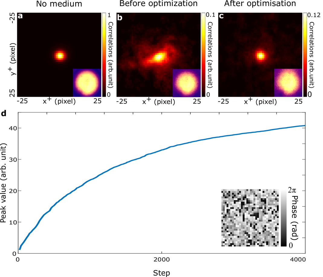
Figure 3: Optimization process. Correlation images measured experimentally using a maximally entangled two-photon state at the input (‘guide state’) without the scattering medium (a), with the scattering medium and before optimization (b), and after optimization (c). d, Optimization curve, showing the variation of the central value in the correlation image in function of the number of steps. The optimization is performed computationally by simulating the experiment on a computer using experimentally measured transmission matrix and two-photon input state. The optimization converges towards an SLM phase mask (inset) that is then used experimentally to tailor the scattering medium.

Tailoring optical disorder

To understand how $S^{\prime}$ is implemented, we first examine the two-photon wavefunction in the input plane:

$${\psi^{\text{in}}}({\mathbf{r_{i}},\mathbf{r_{s}}})={t}\left(\frac{\mathbf{r_{i}}+\mathbf{r_{s}}}{M}\right)\exp{\frac{-|\mathbf{r_{i}}-\mathbf{r_{s}}|^{2}\pi^{2}\sigma_{\mathbf{r}}^{2}}{4\lambda_{p}^{2}f_{1}^{2}}},$$ (3)

where $\mathbf{r_{i}}$ and $\mathbf{r_{s}}$ are the idler and signal photons transverse positions, $M=2f_{1}/f_{0}$ is a magnification factor, ${t}$ is the encoded object function, $\sigma_{\mathbf{r}}=\sqrt{2L\lambda_{p}/(3\pi)}$ is the position correlation width, $\lambda_{p}$ the pump wavelength in the crystal and $L$ its thickness (derivation of Equation (3) is provided in Supplementary Section III, based on the general formalism of Ref. [45]). Then, we make the assumption that $L$ is sufficiently small such that $\sigma_{\mathbf{r}}\approx 0$. The output wavefunction after propagation through the optical transformation $S^{\prime}$ simplifies as:

$$\psi^{\text{out}}({\mathbf{r_{i}^{\prime}},\mathbf{r_{s}^{\prime}}})=\int t(\mathbf{r_{+}})H_{s^{\prime}}(\mathbf{r_{i}^{\prime}},\mathbf{r_{s}^{\prime}},{\mathbf{r_{+}}})d\mathbf{r_{+}},$$ (4)

where $H_{s^{\prime}}(\mathbf{r_{i}^{\prime}},\mathbf{r_{s}^{\prime}},{\mathbf{r_{+}}})=\int s^{\prime}(\mathbf{r_{i}^{\prime}},M\mathbf{r_{+}}/2+\mathbf{r_{-}})s^{\prime}(\mathbf{r_{s}^{\prime}},M\mathbf{r_{+}}/2-\mathbf{r_{-}})d\mathbf{r_{-}}$, $s^{\prime}$ is the coherent point spread function (PSF) associated with $S^{\prime}$, $\mathbf{r_{i}^{\prime}}$ and $\mathbf{r_{s}^{\prime}}$ are idler and signal photons transverse positions in the output plane, respectively. Under this assumption, a class of non-trivial functions $s^{\prime}$ can be found that restore the object image at the output, and are written as:

$$s_{g}^{\prime}(\mathbf{r^{\prime}},\mathbf{r})=\mathcal{F}\{\operatorname{sign}(g)\}(\mathbf{r^{\prime}}-\mathbf{r}),$$ (5)

where $\mathcal{F}$ is the Fourier transform, $g(\mathbf{r})\in\mathbb{R}$ is an arbitrary function and $\operatorname{sign}(g)=1$ if $g>0$, and $-1$ otherwise. Each solution is thus a function of $\mathbf{r}-\mathbf{r}^{\prime}$ whose Fourier transform is a discontinuous function taking values 1 and -1 (i.e. phases 0 and $\pi$) randomly distributed in the transverse plane. By selecting a function $g$ and applying Equation (5), one can construct a non-trivial optical transformation $S^{\prime}$ that renders the system transparent to quantum-encoded images. Because $g$ can be chosen arbitrarily, this approach yields an infinite number of possible solutions. See Methods and Supplementary Section XIII for more details.

In our experiment, however, (i) the approximation $\sigma_{\mathbf{r}}\approx 0$ is not satisfied (see Supplementary Section IX), and (ii) we use a single SLM, which prevents arbitrary tailoring of the transformation $S\rightarrow S^{\prime}$. The general solutions given by Equation (5) are therefore not only approximate but also difficult to implement. Still, they are essential, as they guide our practical implementation of $S^{\prime}$. To achieve this, we first restrict ourselves to the case of thin complex media (e.g. a parafilm layer). Indeed, such media provide a complex but shift-invariant PSF over a wide FOV, a property shared by the solutions of Equation (5). The case of thicker media is discussed in Figure 4 and Supplementary Section IV and X. Then, we use an iterative optimization approach to determine $S^{\prime}$. A two-photon ‘guide state’ is prepared at the input by removing both the object and the $f_{0}$ lens. This state closely approximates the maximally entangled state i.e. $\int a^{\dagger}(\mathbf{r})a^{\dagger}(-\mathbf{r})\ket{0}d\mathbf{r}$ and, as shown in Figure 3a, produces a sharp peak at the center of the correlation image when no medium is present. After propagation through the complex medium, the peak becomes diffuse and significantly broadened (Fig. 3b). To restore it, we use a partitioning algorithm on the SLM [46]. By analogy with classical methods [9, 8], the maximally entangled state effectively acts as a ‘guidestar’ in the correlation image, which the optimization process seeks to restore. Finally, we observe that this process drives the system toward a non-trivial matrix $S^{\prime}$, closely resembling one of the solutions of Equation (5). A detailed comparison between the experimental solutions and those derived from Equation (5) is provided in Supplementary Section X.

While experimentally feasible, this procedure is time-consuming (see Supplementary Section VIII), which motivates our choice to perform the optimization numerically. To do so, we simulated the experiment by propagating the input state through a scattering matrix $S$, both of which were previously measured experimentally, and optimized a virtual SLM. Once an optimal phase pattern is found, it is then programmed on the real SLM, enabling the recovery of a sharp peak in the output correlation image (Fig. 3c). Figure 3d presents the optimization curve i.e. the evolution of the correlation value at the target point as a function of iteration steps, along with the final SLM phase mask. Further details are provided in the Methods and Supplementary section VI.

Demonstration in other complex media

To evaluate the versatility of our method, we applied it to various objects and different types of complex media. For example, Figures 4a,e and i show the measured correlation and intensity images obtained through a random phase mask displayed on the SLM (instead of the physical parafilm layer), where the level of disorder can be precisely controlled. In this case as well, the system becomes transparent to quantum correlations while remaining opaque in classical intensity imaging (Fig. 4c). This effect holds for different levels of disorder, provided that the number of active SLM pixels remains larger than the correlation width of the applied phase mask (see Supplementary Section XII). To better approximate real imaging conditions, we also replaced the scattering layer with a 1-cm-thick layer of polydimethylsiloxane (PDMS), a material commonly used in microscopy to simulate low-order aberrations [47, 48]. Whether placed in a plane conjugate to the SLM (Figs. 4b, f, and j) or in a non-conjugate plane (Figs. 4c, g, and k), our method remains effective, correcting aberrations in the correlation image but not in the classical intensity image. For more complex and thicker media, experiments are challenging to perform due to the very low transmitted photon flux. However, numerical simulations using matrices that reproduce light scattering in thick media show that the approach still works (Figs. 4d, h, and l), albeit over a reduced FOV, similar to that encountered in classical wavefront shaping [9]. The optimized phase masks obtained in these four cases are presented in Supplementary section X.

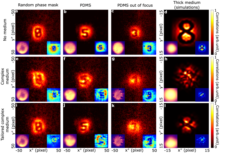
Figure 4: Results for different objects and complex media. Experimental (a-c) and simulated (d) correlation images obtained with different objects and no medium. e-h, Correlation images obtained with the complex medium and no tailoring. Complex media includes a random phase mask with controllable disorder displayed on the SLM (e), a 1-cm-thick layer of polydimethylsiloxane (PDMS) positioned in a plane conjugate to the SLM (f) and out of plane (g), and a simulated thick scattering medium (h). i-l, Correlation images obtained after tailoring the medium. Insets at the bottom left of each panel show intensity images measured under photon-pair illumination; bottom right insets show the corresponding intensity images acquired under classical illumination. Each image is normalized to its maximum value. See Methods for more details on the simulations.

Conclusion

We have demonstrated a method for transmitting images of arbitrary objects through a complex medium using entangled photons. By applying an optimization-based wavefront shaping technique, we tailor the optical disorder to implement a non-trivial transformation that renders the medium transparent to entangled photons, while remaining opaque to classical light.

Quantum entanglement - beyond classical correlations - is essential to our approach, as it enables the preservation of photon correlations across multiple optical bases [49]. This fundamental property is widely exploited in protocols such as entanglement certification and state tomography [50, 51, 52]. In our work, we apply this concept in an imaging context involving two distinct spatial bases: (i) the imaging basis, corresponding to the input image, and (ii) the tailored scattering medium basis $S^{\prime}$. The similarity between the correlation images measured in these two different bases validates the success of our method - a result that cannot be replicated with classically correlated photons, as demonstrated in Supplementary Section XI.

In our approach, the structure of the input states encoding the object - described by Equation (3) - constrains the class of non-trivial solutions $S^{\prime}$ (Eq. (5)). While other solution classes may still exist for the same encoding (but have not been found them), we show in Supplementary Section XIV that using a different encoding, for instance by engineering the nonlinear crystal geometry [53] instead of modulating the pump, leads to a distinct class of non-trivial solutions for $S^{\prime}$. Exploring alternative input state encodings and their associated solution spaces could help overcome limitations encountered here, such as the reduced FOV with increasing medium complexity.

By harnessing the unique physics of non-classical wave propagation in complex media, our work introduces a major conceptual shift by demonstrating that inverting the scattering process is no longer required for imaging. In the near term, this approach promises advances in quantum-secured image transmission through challenging environments such as atmospheric turbulence and mode mixing in fibers, with potential integration of physical unclonable functions for enhanced security [54, 55]. Looking further ahead, our strategy could inspire breakthrough imaging techniques in complex environment, such as biological tissues. It indeed offers multiple accessible solutions (see Supplementary Section XIII) without requiring inversion of the scattering process, and benefits from multimode optimization, which can increase the isoplanatic patch size (i.e. FOV), albeit at the cost of reduced contrast.

Methods

Correlation image. The correlation image $\Gamma^{+}$ is the sum-coordinate projection of the spatial second-order correlation function $G^{(2)}$. To measure it, we use the Tpx3Cam camera, which provides a time-tagged list of photon detection events for each acquisition [56]. Among these events, genuine coincidences are identified as pairs $(x_{i},y_{i},t_{i})$ and $(x_{s},y_{s},t_{s})$ that satisfy $|t_{i}-t_{s}|<6\,\text{ns}$. All other pairs are treated as accidental and discarded. By definition, $G^{(2)}(x_{i},y_{i},x_{s},y_{s})$ is the number of genuine coincidences between the positions $(x_{i},y_{i})$ and $(x_{s},y_{s})$, and $\Gamma^{+}(x_{+},y_{+})$ is the number of such coincidences for which the position sum satisfies $(x_{i}+x_{s},y_{i}+y_{s})=(x_{+},y_{+})$. Formally, the two quantities are related by:

$$\Gamma^{+}(\mathbf{r}_{+})=\iint G^{(2)}(\mathbf{r},\mathbf{r}_{+}-\mathbf{r})\,d\mathbf{r}.$$ (6)

$\Gamma^{+}$ is interpreted as a probability map of the photon-pair barycenter. For example, in the case of near-perfect anti-correlations i.e. when a photon detected at $\mathbf{r}_{i}$ implies its twin is likely at $\mathbf{r}_{s}=-\mathbf{r}_{i}$ - as observed when the object and lens $f_{0}$ are removed - the barycenter remains close to the image center, a sharp peak appears at the center of the correlation image $\Gamma^{+}$. In our work, all correlation images were acquired using acquisition time ranging between $2$s and $30$s. Further details are provided in Supplementary Section II.

Matrix formalism. Assuming that the photon pairs occupy the same polarization and spectral mode, the two-photon state generated by the crystal can be written as:

$$|\psi\rangle=A\iint\psi^{\text{in}}({\mathbf{r_{i}},\mathbf{r_{s}}})a^{\dagger}_{\mathbf{r_{i}}}a^{\dagger}_{\mathbf{r_{s}}}|0\rangle d\mathbf{r_{i}}d\mathbf{r_{s}},$$ (7)

where $A$ is a normalization constant, $\psi^{\text{in}}$ is the spatial two-photon wavefunction, and $\mathbf{r_{i}}=(x_{i},y_{i})$, $\mathbf{r_{s}}=(x_{s},y_{s})$ are the transverse spatial coordinates of the idler and signal photons, respectively, in the input plane. Upon propagation through an arbitrary complex linear optical system, the two-photon wavefunction in the output plane becomes [57]:

$$\psi^{\text{out}}({\mathbf{r_{i}^{\prime}},\mathbf{r_{s}^{\prime}}})=\iint\psi^{\text{in}}({\mathbf{r_{i}},\mathbf{r_{s}}})s(\mathbf{r_{i}^{\prime}},\mathbf{r_{i}})s(\mathbf{r_{s}^{\prime}},\mathbf{r_{s}})d\mathbf{r_{i}}d\mathbf{r_{s}},$$ (8)

where $\psi^{\text{out}}$ is the output wavefunction, $\mathbf{r_{i}^{\prime}}$ and $\mathbf{r_{s}^{\prime}}$ are the transverse positions in the output plane, and $s$ is the coherent point spread function (PSF) of the system. After discretization and ordering of the transverse positions, the wavefunctions $\psi^{\text{in}}$, $\psi^{\text{out}}$, and the PSF $s$ can be represented by matrices $\Psi^{\mathbf{in}}$, $\Psi^{\mathbf{out}}$, and $S$, respectively. Equation (8) then becomes the matrix equation given in Equation (2).

Image encoding. The second-order spatial correlation $G^{(2)}$ in the input plane is obtained by taking the squared modulus of the two-photon field given in Equation (3):

$$G^{(2)}(\mathbf{r_{i}},\mathbf{r_{s}})=\left|t\left(\frac{\mathbf{r_{i}}+\mathbf{r_{s}}}{M}\right)\exp{\frac{-|\mathbf{r_{i}}-\mathbf{r_{s}}|^{2}\pi^{2}\sigma_{\mathbf{r}}^{2}}{4\lambda_{p}^{2}f_{1}^{2}}}\right|^{2}.$$ (9)

The correlation image $\Gamma^{+}$ measured in the camera plane (output plane) without the scattering medium is thus obtained using Equation (6), accounting for the magnification $M^{\prime}$ between the input and output planes:

$$\Gamma^{+}(\mathbf{r_{+}})\approx C\left|t\left(\frac{\mathbf{r_{+}}}{M^{\prime}M}\right)\right|^{2},$$ (10)

where $C$ is a constant. Further details are provided in Refs. [42, 57] and in Supplementary Section III.

Non-trivial solutions $S^{\prime}$. Combining equations (3) and (8), the two-photon field in the output plane can be simplified as:

$$\psi^{\text{out}}({\mathbf{r_{i}^{\prime}},\mathbf{r_{s}^{\prime}}})=\int t(\mathbf{r_{+}})H_{s^{\prime}}(\mathbf{r_{i}^{\prime}},\mathbf{r_{s}^{\prime}},\mathbf{r_{+}})d\mathbf{r_{+}},$$ (11)

where $H$ is defined as:

$$H_{s^{\prime}}(\mathbf{r_{i}^{\prime}},\mathbf{r_{s}^{\prime}},\mathbf{r_{+}}) = \int s^{\prime}\left(\mathbf{r_{i}^{\prime}},\frac{M\mathbf{r_{+}}}{2}+\mathbf{r_{-}}\right)$$ (12)

$$s^{\prime}\left(\mathbf{r_{s}^{\prime}},\frac{M\mathbf{r_{+}}}{2}-\mathbf{r_{-}}\right)$$

$$\exp{\frac{-|\mathbf{r_{-}}|^{2}\pi^{2}\sigma_{\mathbf{r}}^{2}}{\lambda_{p}^{2}f_{1}^{2}}}d\mathbf{r_{-}},$$

where $s^{\prime}$ is the coherent PSF associated with $S^{\prime}$. For $S^{\prime}$ to be a non-trivial solution, $s^{\prime}$ must simultaneously verify:

$$s^{\prime}(\mathbf{r^{\prime}},\mathbf{r})\neq\delta\left(\mathbf{r^{\prime}}+\alpha\mathbf{r}\right),$$ (13)

and

$$H_{s^{\prime}}(\mathbf{r_{i}^{\prime}},\mathbf{r_{s}^{\prime}},\mathbf{r_{+}})=\delta\left((\mathbf{r_{i}^{\prime}}\pm\mathbf{r_{s}^{\prime}})-\mathbf{r_{+}}\right),$$ (14)

where $\alpha\in[-1,1]$ are arbitrary coefficient taking into account potential magnification. In the limit $\sigma_{\mathbf{r}}\rightarrow 0$, equation (12) simplifies to:

$$H_{s^{\prime}}(\mathbf{r_{i}^{\prime}},\mathbf{r_{s}^{\prime}},\mathbf{r_{+}})=\int s^{\prime}(\mathbf{r_{i}^{\prime}},M\mathbf{r_{+}}/2+\mathbf{r_{-}})\,s^{\prime}(\mathbf{r_{s}^{\prime}},M\mathbf{r_{+}}/2-\mathbf{r_{-}})\,d\mathbf{r_{-}}.$$ (15)

Substituting the general form of $s^{\prime}$ from equation (5) into the expression above yields:

$$H_{s^{\prime}}(\mathbf{r_{i}^{\prime}},\mathbf{r_{s}^{\prime}},\mathbf{r_{+}})=\delta\left(\mathbf{r_{i}^{\prime}}+\mathbf{r_{s}^{\prime}}-M\mathbf{r_{+}}\right),$$ (16)

which, when inserted into equation (11), shows that $\psi^{\text{out}}(\mathbf{r_{i}^{\prime}},\mathbf{r_{s}^{\prime}})=t((\mathbf{r_{i}^{\prime}}+\mathbf{r_{s}^{\prime}})/M)$; that is, the object is perfectly restored at the output. See Supplementary Sections III and XIV for more details.
Numerical simulations. All numerical simulations were performed using MATLAB. The input states were propagated via matrix multiplication following the formalism described in Equation (2). To optimize computation time, the simulations were carried out on a discretized transverse space of size less than $51\times 51$ pixels, resulting in matrices of size $2601\times 2601$. Unless otherwise specified, both the input state $\Psi^{\text{in}}$ and the propagation matrix $S$ used in the simulations were experimentally characterized beforehand to closely match the experimental conditions. Further details on the numerical simulations are provided in Supplementary Sections IV.

Optimization process. The optimization process is used to determine the SLM phase mask that implements the optical transformation $S^{\prime}$. It is carried out by numerically simulating the experiment, following an initial experimental characterization phase.
First, the input state - corresponding to the state produced at the output of the crystal without the object and lens $f_{0}$ - is characterized experimentally from spatial correlation measurements in both the input and SLM planes, following the methods described in Refs. [58, 43, 44]. The state is then modeled as a Double-Gaussian distribution [59] and discretized into two matrices $\Psi^{\text{in}}$ and $\Psi^{\text{SLM}}$, the former describing the state in the input plane and the latter in the SLM plane. Second, the matrix $S_{m}$ that links the SLM plane to the output plane (i.e. including the scattering medium) is experimentally measured. For this, the SLM is discretized into $32\times 32$ macropixels, and the matrix is obtained using a classical coherent light source following the method described in Ref. [19]. This measurement enables us to construct the full imaging system matrix i.e. the matrix that links the input to the output plane, denoted $S^{\prime}$. It is given by the product $S^{\prime}=S_{m}D_{\text{SLM}}F_{f_{1}}$, where $D_{\text{SLM}}$ is a diagonal phase matrix representing the action of the SLM, and $F_{f_{1}}$ is a discrete Fourier transform performed by the lens $f_{1}$.
Following this characterization phase, the optimization consists of numerically propagating the input state $\Psi^{\text{in}}$ through the optical system $S^{\prime}$ using Equation (2), for various phase masks displayed on the virtual SLM - that is, by modifying the phase terms in $D_{\text{SLM}}$ - in order to optimize a target in the output correlation image. In practice, to minimize numerical errors introduced by the discrete Fourier transform $F_{f_{1}}$, we simulate the propagation of the experimentally measured state in the SLM plane, $\Psi^{\text{SLM}}$, through the system described by $S_{m}$. In this case, the propagation is given by: $\Psi^{\text{out}}=S_{m}D_{\text{SLM}}\Psi^{\text{SLM}}(S_{m}D_{\text{SLM}})^{t}$. At each optimization step, half of the SLM macropixels - randomly selected - are modulated with a phase delay swept from $0$ to $2\pi$ in 7 steps. This is known as a partitioning algorithm [46]. For each phase value, the numerical propagation is performed, and the central value of the output correlation image, noted $\Gamma^{+}_{0}$, is recorded. As shown in Ref. [38], these data are fitted with the function $a\cos(\theta+\theta_{a})+b\cos(2\theta+\theta_{b})+c$ where $a$, $b$, $c$, $\theta_{a}$, and $\theta_{b}$ are fitting parameters, and $\theta$ is the applied phase shift. The phase shift $\theta_{opt}$ that maximizes this function is then applied to all pixels in the selected group. The procedure is repeated iteratively with new randomly selected subsets of pixels.
At each step, the central peak value of the correlation image increases. As shown in Figure 4d, approximately $4000$ optimization steps are required to reach a plateau. At the end of the optimization, a phase pattern $D_{\text{SLM}}$ that maximizes the correlation peak is obtained, thereby realizing the transformation $S^{\prime}$. This phase pattern is then programmed onto the SLM in the real experiment, assuming that the experimental conditions remain stable over the tens of minutes required for performing the numerical optimization. Further details on the optimization procedure, as well as the experimental characterization of the input state and scattering matrix, are provided in Supplementary Sections V, VI and VII.

Data availability

Data are available from the corresponding author upon reasonnable request.

Author Contributions

C.V. analyzed the data, designed and performed the experiments, with support from B.C. and R.G. C.V. and H.D. conceived the original ideal. All authors discussed the results and contributed to the manuscript. H.D supervised the project.

References

- Davies and Kasper [2012] R. Davies and M. Kasper, Annual Review of Astronomy and Astrophysics 50, 305 (2012).
- Ntziachristos [2010] V. Ntziachristos, Nature Methods 7, 603 (2010), bandiera_abtest: a Cg_type: Nature Research Journals Number: 8 Primary_atype: Reviews Publisher: Nature Publishing Group Subject_term: Microscopy;Optical imaging Subject_term_id: microscopy;optical-imaging.
- Yoon et al. [2020] S. Yoon, M. Kim, M. Jang, Y. Choi, W. Choi, S. Kang, and W. Choi, Nature Reviews Physics 2, 141 (2020).
- Bertolotti and Katz [2022] J. Bertolotti and O. Katz, Nature Physics 18, 1008 (2022).
- Cao et al. [2022] H. Cao, A. P. Mosk, and S. Rotter, Nature Physics 18, 994 (2022).
- Rotter and Gigan [2017] S. Rotter and S. Gigan, Reviews of Modern Physics 89, 015005 (2017), publisher: American Physical Society.
- Vellekoop and Mosk [2007] I. M. Vellekoop and A. P. Mosk, Optics Letters 32, 2309 (2007).
- Horstmeyer et al. [2015] R. Horstmeyer, H. Ruan, and C. Yang, Nature Photonics 9, 563 (2015), number: 9 Publisher: Nature Publishing Group.
- Katz et al. [2012] O. Katz, E. Small, and Y. Silberberg, Nature Photonics 6, 549 (2012), number: 8 Publisher: Nature Publishing Group.
- Yeminy and Katz [2021] T. Yeminy and O. Katz, Science Advances 7, eabf5364 (2021), publisher: American Association for the Advancement of Science.
- Haim et al. [2025] O. Haim, J. Boger-Lombard, and O. Katz, Nature Photonics 19, 44 (2025), publisher: Nature Publishing Group.
- Daniel et al. [2019] A. Daniel, D. Oron, and Y. Silberberg, Optics Express 27, 21778 (2019), publisher: Optica Publishing Group.
- Boniface et al. [2020] A. Boniface, J. Dong, and S. Gigan, Nature Communications 11, 6154 (2020), publisher: Nature Publishing Group.
- Thendiyammal et al. [2020] A. Thendiyammal, G. Osnabrugge, T. Knop, and I. M. Vellekoop, Optics Letters 45, 5101 (2020), publisher: Optical Society of America.
- Freund et al. [1988] I. Freund, M. Rosenbluh, and S. Feng, Physical Review Letters 61, 2328 (1988), publisher: American Physical Society.
- Badon et al. [2020] A. Badon, V. Barolle, K. Irsch, A. C. Boccara, M. Fink, and A. Aubry, Science Advances 6, eaay7170 (2020), publisher: American Association for the Advancement of Science Section: Research Article.
- Boniface et al. [2019] A. Boniface, B. Blochet, J. Dong, and S. Gigan, Optica 6, 1381 (2019), publisher: Optica Publishing Group.
- Kupianskyi et al. [2024] H. Kupianskyi, S. A. R. Horsley, and D. B. Phillips, Optica 11, 101 (2024), publisher: Optica Publishing Group.
- Popoff et al. [2010a] S. M. Popoff, G. Lerosey, R. Carminati, M. Fink, A. C. Boccara, and S. Gigan, Phys. Rev. Lett. 104, 100601 (2010a).
- Popoff et al. [2010b] S. Popoff, G. Lerosey, M. Fink, A. C. Boccara, and S. Gigan, Nature Communications 1, 81 (2010b).
- Liutkus et al. [2014] A. Liutkus, D. Martina, S. Popoff, G. Chardon, O. Katz, G. Lerosey, S. Gigan, L. Daudet, and I. Carron, Scientific Reports 4, 5552 (2014), publisher: Nature Publishing Group.
- Bertolotti et al. [2012] J. Bertolotti, E. G. van Putten, C. Blum, A. Lagendijk, W. L. Vos, and A. P. Mosk, Nature 491, 232 (2012).
- Katz et al. [2014] O. Katz, P. Heidmann, M. Fink, and S. Gigan, Nature Photonics 8, 784 (2014).
- Wu et al. [2016] T. Wu, O. Katz, X. Shao, and S. Gigan, Optics Letters 41, 5003 (2016), publisher: Optica Publishing Group.
- Li et al. [2018a] S. Li, M. Deng, J. Lee, A. Sinha, and G. Barbastathis, Optica 5, 803 (2018a), publisher: Optica Publishing Group.
- Li et al. [2018b] Y. Li, Y. Xue, and L. Tian, Optica 5, 1181 (2018b), publisher: Optica Publishing Group.
- Caramazza et al. [2019] P. Caramazza, O. Moran, R. Murray-Smith, and D. Faccio, Nature Communications 10, 2029 (2019), publisher: Nature Publishing Group.
- Yaqoob et al. [2008] Z. Yaqoob, D. Psaltis, M. S. Feld, and C. Yang, Nature Photonics 2, 110 (2008).
- Tang et al. [2012] J. Tang, R. N. Germain, and M. Cui, Proceedings of the National Academy of Sciences 109, 8434 (2012).
- Papadopoulos et al. [2017] I. N. Papadopoulos, J.-S. Jouhanneau, J. F. A. Poulet, and B. Judkewitz, Nature Photonics 11, 116 (2017).
- Beenakker et al. [2009] C. W. J. Beenakker, J. W. F. Venderbos, and M. P. van Exter, Physical Review Letters 102, 193601 (2009).
- Peeters et al. [2010] W. H. Peeters, J. J. D. Moerman, and M. P. van Exter, Physical Review Letters 104, 10.1103/PhysRevLett.104.173601 (2010).
- Defienne et al. [2016] H. Defienne, M. Barbieri, I. A. Walmsley, B. J. Smith, and S. Gigan, Science Advances 2, e1501054 (2016).
- Valencia et al. [2020] N. H. Valencia, S. Goel, W. McCutcheon, H. Defienne, and M. Malik, Nature Physics 16, 1112 (2020).
- Defienne et al. [2018a] H. Defienne, M. Reichert, and J. W. Fleischer, Physical Review Letters 121, 233601 (2018a), publisher: American Physical Society.
- Courme et al. [2023a] B. Courme, P. Cameron, D. Faccio, S. Gigan, and H. Defienne, PRX Quantum 4, 010308 (2023a).
- Lib et al. [2020] O. Lib, G. Hasson, and Y. Bromberg, Science Advances 6, eabb6298 (2020), publisher: American Association for the Advancement of Science Section: Research Article.
- Courme et al. [2025] B. Courme, C. Vernière, M. Joly, D. Faccio, S. Gigan, and H. Defienne, Non-classical optimization through complex media (2025), arXiv:2503.24283 [quant-ph] .
- van Exter et al. [2012] M. P. van Exter, J. Woudenberg, H. Di Lorenzo Pires, and W. H. Peeters, Phys. Rev. A 85, 033823 (2012).
- Safadi et al. [2023] M. Safadi, O. Lib, H.-C. Lin, C. W. Hsu, A. Goetschy, and Y. Bromberg, Nature Physics , 1 (2023), publisher: Nature Publishing Group.
- Lib and Bromberg [2022] O. Lib and Y. Bromberg, Nature Physics 18, 986 (2022).
- Vernière and Defienne [2024] C. Vernière and H. Defienne, Phys. Rev. Lett. 133, 093601 (2024).
- Defienne et al. [2018b] H. Defienne, M. Reichert, and J. W. Fleischer, In.preparation (2018b).
- Courme et al. [2023b] B. Courme, C. Vernière, P. Svihra, S. Gigan, A. Nomerotski, and H. Defienne, Optics Letters 48, 3439 (2023b).
- Schneeloch and Howell [2016] J. Schneeloch and J. C. Howell, Journal of Optics 18, 053501 (2016).
- Vellekoop and Mosk [2008] I. M. Vellekoop and A. P. Mosk, Optics Communications 281, 3071 (2008).
- Kang et al. [2017] S. Kang, P. Kang, S. Jeong, Y. Kwon, T. D. Yang, J. H. Hong, M. Kim, K.-D. Song, J. H. Park, J. H. Lee, M. J. Kim, K. H. Kim, and W. Choi, Nature Communications 8, 2157 (2017).
- Cameron et al. [2024] P. Cameron, B. Courme, C. Vernière, R. Pandya, D. Faccio, and H. Defienne, Science 383, 1142 (2024), publisher: American Association for the Advancement of Science.
- Spengler et al. [2012] C. Spengler, M. Huber, S. Brierley, T. Adaktylos, and B. C. Hiesmayr, Physical Review A 86, 022311 (2012), publisher: APS.
- Wootters and Fields [1989] W. K. Wootters and B. D. Fields, Annals of Physics 191, 363 (1989).
- Bavaresco et al. [2018] J. Bavaresco, N. Herrera Valencia, C. Klöckl, M. Pivoluska, P. Erker, N. Friis, M. Malik, and M. Huber, Nature Physics 14, 1032 (2018).
- Li et al. [2025] N. K. H. Li, M. Huber, and N. Friis, npj Quantum Information 11, 1 (2025).
- Yesharim et al. [2023] O. Yesharim, S. Pearl, J. Foley-Comer, I. Juwiler, and A. Arie, Science Advances 9, eade7968 (2023).
- Malik et al. [2012] M. Malik, O. S. Magaña-Loaiza, and R. W. Boyd, Applied Physics Letters 101, 241103 (2012), publisher: American Institute of Physics.
- Goorden et al. [2014] S. A. Goorden, M. Horstmann, A. P. Mosk, B. Škorić, and P. W. H. Pinkse, Optica 1, 421 (2014).
- Nomerotski et al. [2023] A. Nomerotski, M. Chekhlov, D. Dolzhenko, R. Glazenborg, B. Farella, M. Keach, R. Mahon, D. Orlov, and P. Svihra, Journal of Instrumentation 18 (01), C01023, publisher: IOP Publishing.
- Abouraddy et al. [2002] A. F. Abouraddy, B. E. A. Saleh, A. V. Sergienko, and M. C. Teich, JOSA B 19, 1174 (2002).
- Edgar et al. [2012] M. Edgar, D. Tasca, F. Izdebski, R. Warburton, J. Leach, M. Agnew, G. Buller, R. Boyd, and M. Padgett, Nature Communications 3, 984 (2012).
- Fedorov et al. [2009] M. V. Fedorov, Y. M. Mikhailova, and P. A. Volkov, Journal of Physics B: Atomic, Molecular and Optical Physics 42, 175503 (2009).