DualNILM: Energy Injection Identification Enabled Disaggregation with Deep Multi-Task Learning

Abstract

Non-Intrusive Load Monitoring (NILM) offers a cost-effective method to obtain fine-grained appliance-level energy consumption in smart homes and building applications. However, the increasing adoption of behind-the-meter energy sources, such as solar panels and battery storage, poses new challenges for conventional NILM methods that rely solely on at-the-meter data. The injected energy from the behind-the-meter sources can obscure the power signatures of individual appliances, leading to a significant decline in NILM performance. To address this challenge, we present DualNILM, a deep multi-task learning framework designed for the dual tasks of appliance state recognition and injected energy identification in NILM. By integrating sequence-to-point and sequence-to-sequence strategies within a Transformer-based architecture, DualNILM can effectively capture multi-scale temporal dependencies in the aggregate power consumption patterns, allowing for accurate appliance state recognition and energy injection identification. We conduct validation of DualNILM using both self-collected and synthesized open NILM datasets that include both appliance-level energy consumption and energy injection. Extensive experimental results demonstrate that DualNILM maintains an excellent performance for the dual tasks in NILM, much outperforming conventional methods.

I Introduction

Non-Intrusive Load Monitoring (NILM) technique enables disaggregation of total household energy consumption into individual appliance usage patterns [1], offering a cost-effective solution for fine-grained energy monitoring. This capability is increasingly critical for smart grid applications, enabling targeted energy-saving recommendations, supporting demand response programs, and enhancing overall grid efficiency [2]. Traditional NILM methods leverage unique electrical signatures of appliances to infer their operating states from aggregate measurements at the utility meter [3, 4, 5]. The value of accurate appliance-level monitoring becomes particularly pronounced during peak demand periods, where granular consumption insights enable utilities to implement precise demand response strategies and maintain grid stability without costly infrastructure upgrades [6].

However, the rapid adoption of behind-the-meter renewable energy systems, particularly residential solar photovoltaic (PV) installations, fundamentally challenges the core assumptions of conventional NILM methods. Modern residential PV systems’ energy injection patterns can completely dominate household consumption profiles during peak generation periods [7, 5]. This paradigm shift invalidates the traditional assumption that aggregate power measurements represent purely consumptive loads, as behind-the-meter generation creates bidirectional power flows that obscure appliance signatures [8].

The resulting “signal eclipse” phenomenon manifests through multiple interconnected challenges. At the signal level, routine appliance operations become indistinguishable from generation fluctuations. For instance, a refrigerator’s compressor activation, normally visible as a distinct step increase in aggregate power, vanishes when offset by simultaneous solar generation. At the temporal level, natural solar variability driven by cloud transients, atmospheric conditions, and diurnal patterns introduces non-stationary variations that mimic appliance switching events. This creates a perfect storm of ambiguity where traditional pattern recognition catastrophically fails. At the system level, when generation exceeds consumption, the net power flow reversal transforms the mathematical structure of the disaggregation problem from a constrained optimization with unique solutions to an under-determined inverse problem with infinite feasible solutions.

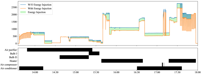
Figure 1: Laboratory measurement of Aggregate power (Watts) showing the impact of micro-inverter energy injection on aggregate power and appliance visibility. The blue line represents aggregate power without injection, orange shows the distorted signal with injection, and green indicates the injected energy. Bottom panels display actual appliance operating states (ON:$\blacksquare$/OFF:$\square$), illustrating how energy injection obscures their detection in the aggregate signal.

The technical complexity of this challenge cannot be overstated. When PV generation exceeds instantaneous consumption, the disaggregation problem undergoes a fundamental mathematical transformation. Traditional NILM benefits from non-negativity constraints that bound the solution space. Each appliance contributes positively to the aggregate, creating a convex optimization landscape. Behind-the-meter generation shatters these constraints, expanding the feasible region to include arbitrary combinations of positive consumption and negative generation that yield identical net measurements. This transformation is further complicated by the electrical characteristics of modern grid-tied inverters, which operate at near-unity power factors to maximize generation efficiency. While optimal for energy production, this operational mode eliminates the reactive power signatures that traditionally help distinguish different load types, removing a critical disambiguation channel just when it is most needed.

Figure 1 empirically demonstrates these theoretical challenges through controlled laboratory experiments. Our micro-inverter injection setup reveals how even modest energy generation fundamentally distorts the aggregate signal morphology. During injection periods (shown in green), the expected additive structure of load aggregation breaks down entirely. The aggregate signal (orange) deviates dramatically from the consumption-only baseline (blue), while the actual appliance states (bottom panels) become completely obscured. This controlled demonstration validates that the challenge transcends simple noise addition; it represents a fundamental incompatibility between conventional NILM architectures and the bidirectional power flows increasingly common in modern residential settings.

To address these challenges, we propose DualNILM, a deep multi-task learning framework specifically designed for simultaneous appliance state recognition and energy injection disaggregation. Our key insight is that generation and consumption, rather than being antagonistic signals, contain complementary information that can be leveraged for mutual disambiguation. The framework integrates sequence-to-point learning for discrete appliance state detection with sequence-to-sequence modeling for continuous injection estimation, unified through a Transformer-based architecture that captures both short-term switching events and long-term generation trends. Critically, DualNILM natively processes multi-channel feature sequences, incorporating active power, reactive power, and extensible to additional electrical signatures. This design exploits cross-dimensional correlations to resolve ambiguities intractable in single-channel analysis. The attention mechanism dynamically weights these feature channels based on the instantaneous generation-consumption balance, effectively performing context-aware feature selection.

Our main contributions are:

• Systematic characterization of the behind-the-meter challenge: We provide rigorous analysis of how residential-scale PV injection fundamentally transforms the NILM problem from constrained optimization to under-determined inverse problem, identifying specific failure modes including signal eclipse effects, temporal aliasing, and constraint relaxation pathologies.

• Novel dual-task architecture with adaptive multi-feature fusion: We present DualNILM, which jointly optimizes appliance state recognition and energy injection estimation through complementary neural pathways. The architecture’s native multi-channel processing with attention-based feature weighting enables robust disaggregation even when generation completely dominates consumption signals.

• Comprehensive validation across diverse operational regimes: Through experiments spanning controlled laboratory environments (500W micro-inverter) and synthetic augmentation with realistic residential-scale generation (2kW PV), we demonstrate DualNILM’s ability to effectively identify appliances’ state and the behind-the-meter injection.

• Open research infrastructure: We release the synthetic PV-augmented versions (with realistic weather data) of REDD and UK-DALE datasets and the corresponding benchmark suites to facilitate continued research in this critical area.

The significance of this work extends beyond addressing an immediate technical challenge. With global residential solar capacity projected to exceed 5.5 TW by 2030, representing a threefold increase from 2023 levels [9, 10], the ability to maintain load visibility despite bidirectional power flows becomes critical infrastructure for grid intelligence. The dual-task paradigm we propose provides a scalable framework naturally extensible to emerging energy scenarios involving battery storage, vehicle-to-grid systems, and peer-to-peer energy trading. By demonstrating that generation and consumption can be simultaneously tracked using existing smart meter infrastructure, without requiring expensive smart inverters or dedicated generation meters, this work democratizes access to advanced energy analytics and accelerates the transition toward a truly intelligent and sustainable energy future.

The rest of the paper is organized as follows. Section II discusses and gives the literature on related work. Section III presents the problem formulation and highlights the challenge. Section IV details our proposed DualNILM framework. Section V describes the experimental setup, including the realistic energy injection data simulation, and Section VI presents the experimental results and analysis. Finally, Section VII concludes the paper and discusses future directions.

II Related work

II-1 Evolution of NILM Technique

Non-Intrusive Load Monitoring (NILM) has been a subject of extensive research since its introduction by Hart [1]. Traditional NILM approaches rely on identifying unique appliance signatures in the aggregate power signal to disaggregate individual appliance usage [3]. Techniques such as Hidden Markov Models (HMMs) [11], factorial HMMs [12], and combinatorial optimization [13] have been widely used. With the advent of deep learning, neural network-based methods have significantly advanced NILM performance. Convolutional Neural Networks (CNNs) and Recurrent Neural Networks (RNNs) have been employed to capture temporal dependencies and extract features from power signals [14, 15, 16]. Sequence-to-point and sequence-to-sequence models have been proposed to improve disaggregation accuracy [15, 17]. Recently, researchers have also introduced advanced deep architectures, such as transformer-based models and graph neural networks, to further enhance disaggregation performance [18, 19]. These approaches leverage long-range temporal context and inter-appliance relationships to achieve higher accuracy on benchmark datasets while improving the generalization ability of NILM models.

II-2 Categories of NILM Methods

NILM methods can also be categorized based on their task-oriented objectives. Many approaches focus on event-based detection, where the key aim is to recognize appliance switching events (ON/OFF transitions) and label those events with the corresponding device [20, 21]. This category typically relies on detecting changes in aggregate power that exceed a certain threshold, followed by a classification stage to identify which appliance caused the event. Various improvements to event detection have been proposed, including hybrid schemes that combine primary event triggers with secondary verification algorithms to reduce false detections [22]. By isolating transition points in the time series, event-based NILM methods can be highly interpretable and computationally efficient, but they may struggle with appliances that exhibit gradual power variations or multiple internal states [23]. On the other hand, the steady-state-based approaches emphasize continuous monitoring of power consumption, estimating the exact load of each device over time. These NILM methods often employ more complex models (e.g., HMMs or deep neural networks) and can capture multi-level operating states of appliances [24].

II-3 NILM Methods amid RE Integration

Previous work addressing NILM with renewable energy integration is limited. In [25], the authors investigate methods to manage power injection systems in renewable setups, emphasizing system stability. Similarly, Aygen et al. [26] consider a zero-sequence current injection technique for mitigating unbalanced loads in systems integrated with renewables, which, however, is not directly applicable to NILM. Only a few studies have attempted to explicitly disaggregate solar generation from the net metered signal. Noori et al. [27] recently examined solar disaggregation and highlighted that incorporating external context like solar irradiance can improve the detection of solar generation. In [8], the authors investigate solar energy disaggregation but rely on high-frequency data and additional features, which may not be practical in real-world deployments. Other studies have considered the use of additional sensors or prior knowledge of the energy injection [28], which limits their applicability.

Our work differs from existing approaches by explicitly addressing the challenge of energy injection in NILM using a deep multi-task learning framework. By simultaneously performing appliance state recognition and energy injection disaggregation, our proposed DualNILM effectively handles the complexities introduced by RE sources without relying on additional sensors or impractical data requirements.

III Challenge and Problem Formulation

This section clarifies the underlying NILM challenge when a portion of the household power flow originates from behind-the-meter sources, such as micro-inverters or PV and battery storage. We start by revisiting the traditional NILM setup and note its known complexity. Subsequently, we describe how negative (export) flows from renewable micro-inverters break the standard constraints, broadening the search space and hindering standard disaggregation techniques. Then, we introduce the DNN-based NILM with extra features and propose a multi-task formulation—covering both conventional appliances and a dedicated injection channel—that motivates modern deep-learning solutions to this harder scenario.

III-A Motivation and Overview

Traditional NILM approaches aim to infer appliance-level power consumption from aggregated household measurements, typically under the assumption that all loads are strictly nonnegative [1, 13]. In practice, however, many residences now include small-scale renewable generation (e.g., rooftop solar). The micro-inverter responsible for turning this generation into usable AC power can appear as a “negative appliance” from the meter’s perspective whenever produced electricity exceeds local consumption.

In our laboratory studies, the introduction of even a modest 500 W micro-inverter often distorted the aggregate load profile enough to render certain appliance signatures indistinct (see Fig. 1). This distortion led to substantially higher disaggregation error for methods that assume strictly nonnegative loads, as evidenced in Table III. Moreover, the difficulty can be exacerbated by low sampling rates or the lack of multi-feature data, both common in real-world metering systems [14, 5].

III-B Classic Single-Blind NILM

Let $y(t)$ be the aggregate power at time $t$, and assume there are $N$ distinct appliances. Denote $s_{n}(t)\in\{0,1\}$ as the on/off state of the $n$-th appliance and $x_{n}(t)\geq 0$ as its power consumption when active. In this classical viewpoint, the total load is

$$y(t)\;=\;\sum_{n=1}^{N}s_{n}(t)\,x_{n}(t)\;+\;\epsilon(t),$$ (1)

where $\epsilon(t)$ is measurement noise. Equivalently, over a horizon of length $T$,

$$\mathbf{y}\;=\;\sum_{n=1}^{N}\Bigl(\mathbf{s}_{n}\odot\mathbf{x}_{n}\Bigr)\;+\;\boldsymbol{\epsilon},$$

with $\mathbf{y},\,\mathbf{x}_{n},\boldsymbol{\epsilon}\in\mathbb{R}^{T}$ and $\mathbf{s}_{n}\in\{0,1\}^{T}$. Since NILM typically focuses on a smaller subset of $K$ target appliances, the remainder of the loads can be aggregated into a single term $v(t)$, as in

$$y(t)\;=\;\sum_{n=1}^{K}s_{n}(t)\,x_{n}(t)\;+\;v(t).$$ (2)

Solving for $\{s_{n}(t),x_{n}(t)\}$ is known to be NP-hard in general [1], but the purely nonnegative structure has historically allowed heuristic or machine-learning-based methods to achieve acceptable performance [3, 4, 2].

III-C When Negative Flows Disrupt Classical NILM

As household renewable penetration increases, at least one “appliance” (the micro-inverter) can feed power back to the grid, producing negative net load. The aggregated signal then becomes

$$y(t)\;=\;\sum_{n=1}^{N-1}\Bigl[s_{n}(t)\,x_{n}(t)\Bigr]\;+\;\underbrace{s_{k}(t)\,x_{k}(t)}_{\text{behind-the-meter injection}}\;+\;\epsilon(t),$$

where the $k$-th device’s power, $x_{k}(t)$, may be negative at some time points.

III-C1 Why Behind-the-Meter Injection Complicates NILM (a Theoretical Signal Processing Perspective)

In the language of signal processing and blind source separation (BSS), classical NILM can be viewed as a single-channel mixture of purely nonnegative sources. The geometry of such mixtures is conic: if each device’s load lies in the nonnegative orthant, standard factorization approaches (e.g., nonnegative matrix factorization) can leverage convexity to help isolate distinct appliance patterns [29].

Once one or more sources are allowed to take negative values (e.g., exporting solar power), the total load no longer resides in the same conic space. Mathematically, the feasible solution set expands:

$$\mathcal{F}_{\text{injection}}=\;\Bigl\{(\mathbf{s},\mathbf{x}):\mathbf{x}_{n}\in\mathbb{R}_{+}^{T},\,\mathbf{x}_{k}\in\mathbb{R}^{T},\,\mathbf{y}=\sum_{n=1}^{N-1}\bigl(\mathbf{s}_{n}\odot\mathbf{x}_{n}\bigr)+\bigl(\mathbf{s}_{k}\odot\mathbf{x}_{k}\bigr)\Bigr\}.$$

Because one column (the injection device) spans a broader region than the nonnegative orthant, various identifiability arguments from conic geometry and nonnegative matrix factorization lose traction. In essence:

• Larger Search Space: With fewer constraints, multiple plausible ways to explain any observed dip or negative interval emerge, inflating ambiguity.

• Broken Uniqueness: Nonnegative factorizations often depend on convexity-based uniqueness results; negative entries undermine these results and can make standard disaggregation fall back on naive assumptions.

• Low-Dimensional Data Shortcomings: If the meter only provides a single power reading or a low-resolution signal, there is insufficient structure to separate negative flows from positive loads, compounding the difficulty.

Consequently, traditional NILM methods that treat all loads as nonnegative typically fail to disentangle consumption from behind-the-meter generation when measurements dip below zero or remain subdued for extended intervals. Figure 1 highlights how the micro-inverter depresses the net power curve, obscuring appliance signatures; Table III further illustrates that classical NILM approaches suffer markedly when negative flows are not accounted for, especially under limited feature sets or learning capacity. More discussion of the theoretical analysis is given in Appendix A.

III-D DNN-Based Approaches and Richer Feature Spaces

Deep learning methods, ranging from different artificial neural networks, have demonstrated promise for NILM by exploiting additional data dimensions (e.g., voltage, current, reactive power) or learning more expressive latent representations [14, 15, 30]. Formally, let $\mathbf{f}(t)\in\mathbb{R}^{F-1}$ denote supplementary measurements at time $t$ (with $F$ being the total feature dimension if one counts active power as well). A neural model can then be structured as

$$[\hat{s}_{n},\,\hat{x}_{n}]\;=\;\mathrm{DNN}_{\theta}\bigl([\mathbf{y},\,\mathbf{f}]\bigr),\quad n=1,\dots,K,$$ (3)

where $\theta$ are trainable parameters. In scenarios where the meter data are more comprehensive (e.g., capturing phase angles or higher sampling rates), the negative injection component can be learned as a distinct pattern. However, when only low-dimensional features are available, the challenge described in Section III-C remains severe, necessitating specialized modeling.

III-E A Multi-Task Formulation for Injection and Appliance Disaggregation

A practical way to handle negative flows is to treat the micro-inverter (or any injecting source) as a separate “task” alongside conventional appliances. Specifically, if $K$ total devices are considered, define the $k$-th as the injection device with $x_{k}(t)\in\mathbb{R}$. Then, a hybrid multi-task network can produce:

$$\Bigl[\hat{s}_{1},\ldots,\hat{s}_{K},\;\hat{x}_{k}\Bigr]\;=\;\mathrm{DNN}_{\theta}\!\bigl(\mathbf{y},\,\mathbf{f}\bigr),$$ (4)

where $\hat{x}_{k}$ explicitly models the behind-the-meter source. This architecture allows leveraging correlations between appliance load patterns and injection events (e.g., solar generation peaks), enforcing physical constraints such as capacity limits, and ultimately improving interpretability.

III-F Key Takeaways

1. Classical Single-Blind NILM: Cast as an NP-hard but structured problem in which nonnegative loads provide some conic geometric constraints.

2. Behind-the-Meter Injection: Relaxing nonnegativity for at least one source broadens the solution set, complicates identifiability, and necessitates a refined treatment in order to avoid large errors.

3. Towards a Multi-Task Solution: Leveraging multi-feature data, explicit modeling of the injecting source, and modern deep architectures can partially restore identifiability and improve real-world performance.

The next section introduces our proposed methodology, which exploits these insights by combining sequence-to-point and sequence-to-sequence deep learning strategies while explicitly modeling injection as a dedicated task.

IV DualNILM

To address the challenges outlined in Section III, we propose DualNILM, a novel deep multi-task learning framework for simultaneous energy disaggregation and injection identification. This section details the architecture of DualNILM, its key components, and the motivations behind our design choices. More implementation details can be found in Appendix. B.

IV-A Method Overview and Design Rationale

In Section III, we established that behind-the-meter negative power flows from micro-inverters expand the solution space beyond the typical nonnegative constraint, compounding disaggregation ambiguity. DualNILM mitigates this difficulty by:

• Separately Modeling Injection: Instead of forcing a single model head to predict all appliance consumptions (including negative flows), we assign a distinct output channel for the injection source. This explicit handling of negative values helps isolate the behind-the-meter signal from conventional appliances.

• Multi-Scale Feature Extraction: Appliance usage patterns often manifest as short-term events (e.g., on/off transients) superimposed on longer-term trends, whereas injection can exhibit relatively smooth variations (e.g., daily solar generation). To capture both fine-grained patterns and global context, DualNILM combines convolutional layers (for local feature learning) with Transformer layers (for longer-range sequence dependencies).

• Multi-Task Optimization: The model jointly learns to classify appliance states (binary on/off) and predict the magnitude of the injected power. This multi-task approach leverages shared feature representations, improved regularization, and explicit constraints (such as maximum injection capacity) to handle overlapping load signatures more effectively.

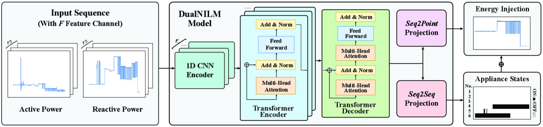
Figure 2: Architecture of DualNILM

IV-B Model Architecture

The overall architecture of DualNILM is illustrated in Fig. 2. Our model comprises four main components: 1) CNN encoders, 2) transformer encoders, 3) a transformer decoder, and 4) task-specific projection layers. This design allows for the effective capture of both local and global temporal dependencies in the power consumption patterns while enabling multi-task learning.

IV-B1 CNN Encoders

The input to our model is a multi-channel time series $\mathbf{X}\in\mathbb{R}^{T\times F}$, where $T$ is the sequence length and $F$ is the number of input features (e.g., active power, reactive power). We employ a separate 1D CNN Encoder for each feature channel to extract local temporal patterns. Each CNN Encoder consists of multiple 1D convolutional layers interleaved with LayerNorm operations:

$$\mathbf{H}_{f}=\text{CNN}_{f}(\mathbf{X}_{f}),\quad f=1,\ldots,F$$ (5)

where $\mathbf{X}_{f}\in\mathbb{R}^{T}$ is the $f$-th feature channel and $\mathbf{H}_{f}\in\mathbb{R}^{T\times D}$ is the corresponding encoded representation. Using separate CNN Encoders for each feature allows the model to learn feature-specific local patterns, enhancing its ability to capture the unique characteristics of different electrical measurements [14].

IV-B2 Transformer Encoder

The outputs of the CNN Encoders are concatenated along the feature dimension and fed into Transformer Encoders [31]. The Transformer Encoder employs multi-head attention mechanisms to capture long-range dependencies in the input sequence:

$$\mathbf{Z}=\text{TransformerEncoder}([\mathbf{H}_{1};\ldots;\mathbf{H}_{F}])$$ (6)

where $\mathbf{Z}\in\mathbb{R}^{T\times D^{\prime}}$ is the output of the Transformer Encoder. This component allows DualNILM to model complex interactions between different appliances and the energy injection source over time, which is crucial for accurate disaggregation and injection estimation [15].

IV-B3 Transformer Decoder and Task-Specific Projections

To address the dual tasks of appliance state detection and energy injection estimation, we employ a hybrid approach combining sequence-to-point (Seq2Point) and sequence-to-sequence (Seq2Seq) strategies:

• For appliance state detection, we use a Seq2Point approach. The last time step of the Transformer Encoder output is projected to predict the states of certain appliances $i$:

  $$\hat{\mathbf{s_{i}}}=\sigma(\mathbf{W}_{s_{i}}\mathbf{z}_{T}+\mathbf{b}_{s_{i}})$$ (7)

  where $\mathbf{z}_{T}$ is the last time step of $\mathbf{Z}$, $\mathbf{W}_{s_{i}}$ and $\mathbf{b}_{s_{i}}$ are learnable parameters, and $\sigma$ is the sigmoid activation function.

• For energy injection estimation, we employ a Seq2Seq approach using a transformer decoder:

  $$\hat{\mathbf{x}}_{K}=\sigma(\mathbf{W}_{x}\cdot\text{TransformerDecoder}(\mathbf{Z})+\mathbf{b}_{x})$$ (8)

  where $\hat{\mathbf{x}}_{K}\in\mathbb{R}^{T}$ is the predicted energy injection sequence, and $\mathbf{W}_{x}$ and $\mathbf{b}_{x}$ are learnable parameters.

IV-C Highlights of DualNILM

• Robust in Real Settings: Apply LayerNorm [32] instead of normalization for inputs to ensure numerical stability when faced with unscaled, continuous data. In practice, DualNILM can process raw meter readings without mandatory preprocessing, mitigating performance drops due to distributional shifts between training and deployment.

• Scalable & Incremental: Each appliance’s state recognition is handled by its own projection layer, allowing new appliances to be added without retraining the entire network. This modular “add-on” structure preserves performance for existing appliances and only requires fitting new parameters for the introduced appliance.

• Cross-Task Synergy: Jointly modeling appliance states and energy injection helps disentangle negative power flows from reduced consumption. Accurate inverter detection can prevent misclassifying low-usage intervals as “off,” while robust appliance recognition clarifies whether dips in aggregate load stem from actual load decrease or solar export.

Overall, DualNILM integrates CNN-based local feature extraction, transformer-level global context, and dual-task outputs to tackle behind-the-meter injection challenges with stable performance, easy expandability, and improved separation of negative flows.

IV-D Training Objective and Optimization

Denote $\mathbf{Y}$ is the set of ground truth, e.g $(\mathbf{S},\mathbf{X})$. Our optimization target is:

$$\operatorname*{arg\,min}_{\theta}\mathcal{L}(\mathbf{Y},\text{{{DualNILM}}}_{\theta}([\mathbf{y},\mathbf{f}]))$$ (9)

The multi-task nature of DualNILM is reflected in its loss function $\mathcal{L}$, which combines binary classification/recognition loss for appliance state detection and the disaggregation error loss for energy injection estimation:

$$\mathcal{L}=\lambda_{1}\mathcal{L}_{\text{Rec}}(\hat{\mathbf{S}},\mathbf{S})+\lambda_{2}\mathcal{L}_{\text{Disagg}}(\hat{\mathbf{x}}_{K},\mathbf{x}_{K})$$ (10)

where $\lambda_{1}$ and $\lambda_{2}$ are weighting factors to balance the two tasks. The model can be optimized via gradient backpropagation approaches like SGD [33], Adam [34], etc. Specifically, we employ the Dice loss [35], which is particularly effective for imbalanced binary classification problems for appliance state recognition:

$$\mathcal{L}_{\text{Rec}}=\sum_{i=1}^{K}(1-\frac{2|\hat{\mathbf{s_{i}}}\cap\mathbf{s_{i}}|}{|\hat{\mathbf{s_{i}}}|+|\mathbf{s_{i}}|})$$ (11)

For injection estimation, we can use a standard L1 or L2 measure: MAE (Mean Absolute Error) and Mean Square Error (MSE). Note that we can apply constraints/normalization on injection disaggregation targets as the maximum output of micro-inverters or community solar installations often adheres to standardized designed values like EN50583 [36].

V Experimental Setup

To thoroughly evaluate the performance of DualNILM, we conducted extensive experiments using both real-world data collected in our laboratory and simulated data based on widely used public datasets. This section details our experimental setup, including datasets and simulations, evaluation metrics, benchmark methods, and experiment procedures.

V-A Datasets and Simulation

V-A1 Laboratory Dataset

We collected a real-world dataset in our laboratory and conducted extensive experiments. The dataset includes individual power consumption data for multiple appliances and the behind-the-meter energy injection from a micro-inverter. The data was collected from December 6 to December 15, 2023, and was sampled at 2-second intervals using sub-meters for each appliance on both active power and reactive power. The dataset includes the following appliances: i) Air purifier, ii) Heater, iii) Light bulb Type I, iv) Light bulb Type II, v) Air compressor, vi) Air conditioner, vii) Micro-inverter (energy injection). Table. I presents the key statistics of our laboratory dataset.

TABLE I: Statistics of the Laboratory Dataset

Appliance	Mean Power (W)	Std Dev (W)	On-time (%)
Air purifier	34.25	2.35	40.57
Heater	1345.73	476.90	28.69
Light bulb Type I	204.84	13.64	10.54
Light bulb Type II	412.99	49.39	10.59
Air compressor	1408.04	287.72	0.4885
Air conditioner	695.59	82.92	38.61
Micro-inverter	219.31	115.77	63.56
Micro-inverter’s value means the power injection

Furthermore, in our experiments on our laboratory datasets, we perform cross-validation by using data from one day for testing and the data from the remaining days for training, iterating over all days in the dataset.

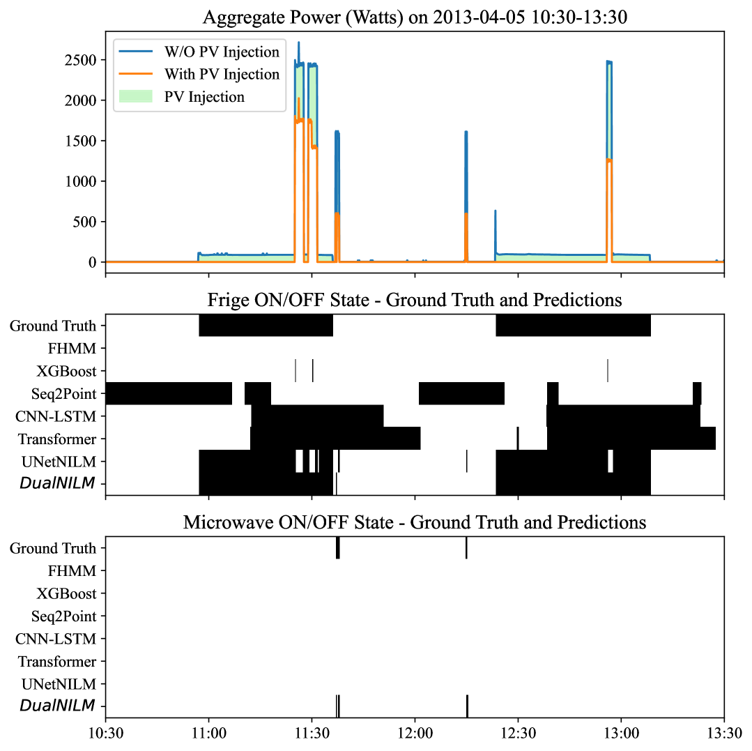
Figure 3: Simulated Photovoltaic energy injection on UKDALE House1 on Apr. 05, 2013, and the corresponding appliances states (ON:$\blacksquare$/OFF:$\square$) for Fridge and Microwave and their predictions from DualNILM and benchmarks.

V-A2 Synthetic Public Datasets

To evaluate the generalizability of DualNILM and facilitate comparison with existing methods, we simulate energy injection scenarios using two widely-used public NILM datasets: REDD [13] and UK-DALE [37]. Our simulation leverages real-world solar irradiance data and photovoltaic (PV) system modeling to create realistic scenarios of residential solar energy injection. The simulation process involved the following steps:

1. Selection of Houses: Select houses from each dataset with suitable appliance combinations. Specifically, we focused on houses with the appliances commonly used in prior works: microwave, fridge, dishwasher, and washing machine for REDD; and kettle, microwave, fridge, dishwasher, and washing machine for UK-DALE.

2. Acquisition of Solar Irradiance Data: We obtain historical solar irradiance data from the National Solar Radiation Database (NSRDB) provided by the National Renewable Energy Laboratory (NREL) [38]. The NSRDB offers detailed solar radiation data, including Global Horizontal Irradiance (GHI), Direct Normal Irradiance (DNI), and Diffuse Horizontal Irradiance (DHI), with a temporal resolution of 30 minutes. We collect data for the rough geographical locations corresponding to the datasets:

   • REDD Location: Boston, MA, USA (Latitude: 42.3601^∘N, Longitude: 71.0589^∘W)

   • UK-DALE Location: London, UK (Latitude: 51.5074^∘N, Longitude: 0.1278^∘W)

3. Simulation of Photovoltaic System Output: Using the collected irradiance data, we simulate a residential PV system with a designed maximum output capacity of 120 W, representing a small-scale household solar installation. The simulation accounts for temperature effects on PV efficiency, following the methods described in [39, 40].

   The cell temperature $T_{\text{cell}}$ is calculated as:

   $$T_{\text{cell}}=T_{\text{ambient}}+\frac{\text{GHI}}{1000}\times\left(\frac{T_{\text{NOCT}}-20}{0.8}\right),$$ (12)

   where $T_{\text{ambient}}$ is the ambient temperature in degrees Celsius, GHI is the Global Horizontal Irradiance in W/m², and $T_{\text{NOCT}}$ is the Nominal Operating Cell Temperature, typically 45^∘C. The efficiency adjustment $\eta_{\text{adj}}$ due to temperature is computed as:

   $$\eta_{\text{adj}}=1+\gamma\times(T_{\text{cell}}-25),$$ (13)

   where $\gamma$ is the temperature coefficient ($-0.005$ ^∘C^-1 for silicon-based PV modules). The PV power output $P_{\text{PV}}$ is then calculated using:

   $$P_{\text{PV}}=\min\left(P_{\text{rated}},\frac{\text{GHI}\times P_{\text{rated}}}{1000}\times\eta_{\text{adj}}\times\eta_{\text{inv}}\right),$$ (14)

   where $P_{\text{rated}}$ is the rated capacity (120 W in our simulation) and $\eta_{\text{inv}}$ is the inverter efficiency (0.96 based on [41]).

4. Reactive Power Simulation: For comprehensive power analysis, we simulate reactive power characteristics for both appliances and the PV system based on typical power factors from industry standards [42]. For each appliance with active power $P$, its reactive power $Q$ is calculated as:

   $$Q=P\times\tan(\arccos(\text{PF}))$$ (15)

   where PF varies by appliance type following established standards [43, 44]: refrigerator (0.85), microwave (0.95), washing machine (0.75), dishwasher (0.80), kettle (0.99), and micro-inverter (0.98).

5. Integration with Household Consumption: We integrate the simulated PV output with the aggregate power consumption data from the datasets. To reflect realistic scenarios where excess generation is not exported to the grid, we cap the PV output at the household’s instantaneous consumption:

   $$P_{\text{PV}}^{\text{adjusted}}=\min\left(P_{\text{PV}},P_{\text{agg}}\right),$$ (16)

   where $P_{\text{agg}}$ is the original aggregate power consumption. The aggregate power with PV injection is then:

   $$P_{\text{agg}}^{\text{injected}}=P_{\text{agg}}-P_{\text{PV}}^{\text{adjusted}}.$$ (17)

   We ensure that $P_{\text{agg}}^{\text{injected}}\geq 0$ by setting any negative values to zero.

Figure 3 demonstrates the challenging disaggregation scenario on UKDALE House 1 during midday hours (10:30-13:30) on April 05, 2013, when PV injection interacts with typical household consumption. The aggregate power exhibits dramatic variations as appliances cycle, yet the PV injection (green shaded area) creates subtle but critical distortions in the net measurement. During periods of low baseline consumption, such as when only the refrigerator operates between switching events, even modest PV generation can mask appliance signatures entirely.

We use the following cross-validation setup for each dataset:

• REDD: Houses 1, 2, and 3: 1-week training, 3-day testing.

• UK-DALE: Houses 1 and 2: 2-week training, 1-week testing.

Table. VI shows the key statistics of our synthetic datasets. More detailed dataset descriptions on both laboratory and simulated public data, including detailed configuration and simulation and appliance state labeling, are described in Appendix. C.

V-B Evaluation Metrics

We employ different metrics to evaluate the performance of DualNILM on appliance state recognition and energy injection estimation tasks.

V-B1 Appliance State Recognition Metrics

For each appliance and the overall model performance, we compute the following metrics:

• Accuracy: The proportion of correct predictions (both true positives and true negatives) among the total number of cases examined.

• Recall: The proportion of actual positive cases that were correctly identified.

• Precision: The proportion of positive identifications that were actually correct.

• F1-score: The harmonic mean of precision and recall, providing a single score that balances both metrics.

These metrics are calculated for each appliance individually and then averaged across all appliances to provide an overall performance assessment. Noted that since the

V-B2 Energy Injection Estimation Metric

For the energy injection estimation task, we use the Root Mean Square Error (RMSE) and Mean Absolute Error (MAE) as the metrics:

$$RMSE =\sqrt{\frac{1}{T}\sum_{t=1}^{T}(x_{K}(t)-\hat{x}_{K}(t))^{2}}$$ (18)

$$MAE =\frac{1}{T}\sum_{t=1}^{T}|x_{K}(t)-\hat{x}_{K}(t)|$$

where $x_{K}(t)$ is the true injection value and $\hat{x}_{K}(t)$ is the estimated injection value at time $t$. These metrics quantify the accuracy of the model’s energy injection estimates over time.

V-C Benchmark Methods

To comprehensively evaluate DualNILM, we compare it with representative and state-of-the-art methods in both appliance state recognition and energy injection disaggregation tasks. Table II summarizes our benchmark methods.

TABLE II: Summary of Benchmark Methods

Category	Method	Key Characteristics	Primary Strengths	Tasks*
Traditional	FHMM [11]	Parallel hidden Markov chains	Interpretable state modeling	Both
	XGBoost [45]	Tree-based ensemble	Non-linear pattern recognition	State Recognition
Deep Learning	Seq2Point [15]	CNN-based architecture	Local temporal features	State Recognition
	CNN-LSTM [46]	Hybrid CNN-LSTM	Local-global temporal modeling	State Recognition
	Transformer [31]	Self-attention mechanism	Long-range dependencies	State Recognition
	Seq2Seq [17]	Encoder-decoder LSTM	Sequence mapping	Disaggregation
	DAE [47]	Denoising autoencoder	Signal reconstruction	Disaggregation
	UNetNILM [48]	Skip-connected encoder-decoder	Multi-task learning	Both
*Tasks include State Recognition (appliance state recognition), Disaggregation (energy injection disaggregation), and Both (both tasks).

For fair comparison and evaluation, we select both traditional NILM methods like FHMM and modern deep learning approaches. While some methods specialize in either appliance state recognition or energy injection disaggregation, methods like FHMM and UNetNILM handle both tasks simultaneously. This diverse selection enables comprehensive evaluation of DualNILM’s performance across different technical approaches and computational paradigms, with particular attention to the unique challenges posed by behind-the-meter energy injection.

Detailed configurations and implementation specifics are provided in Appendix D-A. All benchmark models were implemented with carefully tuned hyperparameters to ensure fair comparison. This comprehensive selection enables evaluation across different technical approaches, with particular attention to methods capable of handling behind-the-meter energy injection.

VI Experimental Results

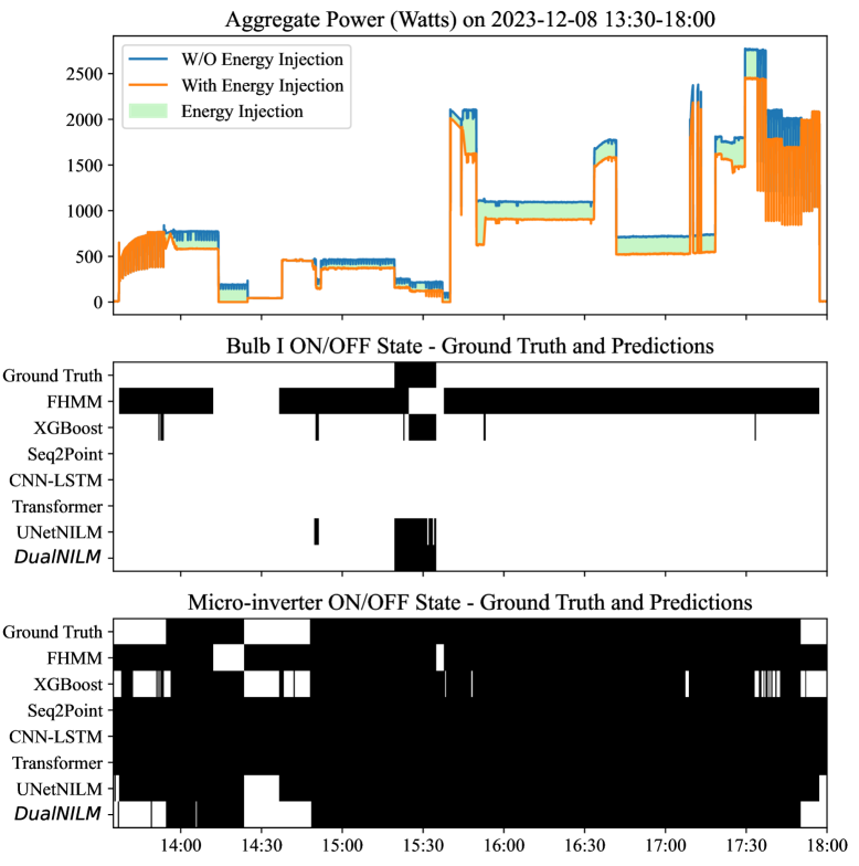
Figure 4: Visualization of Bulb I and Micro-inverter State’s Ground Truth and Predictions across All Benchmark Methods on Dec.8, 2023 of our data (ON:$\blacksquare$/OFF:$\square$).

This section presents comprehensive evaluation of DualNILM across real-world laboratory measurements and synthetic public datasets augmented with PV injection. We analyze performance on controlled micro-inverter injection collected in our laboratory and validate generalization through synthetic augmentation of REDD and UK-DALE datasets, demonstrating the framework’s effectiveness across diverse behind-the-meter injection scenarios.

TABLE III: Overall Avg. Performance Metrics of Appliance State Recognition (Cross-validation on all splits of each Dataset)

Dataset		Method	Accuracy $\uparrow$(%)	Recall $\uparrow$(%)	Precision $\uparrow$(%)	F1 $\uparrow$(%)
Laboratory Dataset (Real Behind-the-Meter Injection)		FHMM	60.95${}_{\scriptstyle\,\pm 27.96}$	28.32${}_{\scriptstyle\,\pm 40.81}$	16.84${}_{\scriptstyle\,\pm 28.20}$	17.25${}_{\scriptstyle\,\pm 27.23}$
		XGBoost	85.82${}_{\scriptstyle\,\pm 2.07}$	48.20${}_{\scriptstyle\,\pm 7.69}$	52.10${}_{\scriptstyle\,\pm 6.02}$	47.75${}_{\scriptstyle\,\pm 6.75}$
		Seq2Point	67.63${}_{\scriptstyle\,\pm 17.08}$	53.06${}_{\scriptstyle\,\pm 10.80}$	27.86${}_{\scriptstyle\,\pm 14.16}$	34.27${}_{\scriptstyle\,\pm 13.29}$
		CNN-LSTM	74.03${}_{\scriptstyle\,\pm 15.51}$	52.97${}_{\scriptstyle\,\pm 11.02}$	30.29${}_{\scriptstyle\,\pm 14.28}$	36.67${}_{\scriptstyle\,\pm 13.25}$
		Transformer	81.79${}_{\scriptstyle\,\pm 12.65}$	52.91${}_{\scriptstyle\,\pm 10.76}$	38.16${}_{\scriptstyle\,\pm 15.53}$	42.76${}_{\scriptstyle\,\pm 14.02}$
		UNetNILM	89.20${}_{\scriptstyle\,\pm 9.76}$	54.01${}_{\scriptstyle\,\pm 27.35}$	60.81${}_{\scriptstyle\,\pm 30.96}$	53.89${}_{\scriptstyle\,\pm 27.00}$
		DualNILM	98.54${}_{\scriptstyle\,\pm 1.71}$	85.43${}_{\scriptstyle\,\pm 28.03}$	84.16${}_{\scriptstyle\,\pm 28.45}$	84.54${}_{\scriptstyle\,\pm 27.93}$
REDD (Synthetic PV Injection)	House 1	FHMM	79.52${}_{\scriptstyle\,\pm 39.21}$	1.46${}_{\scriptstyle\,\pm 3.60}$	13.47${}_{\scriptstyle\,\pm 33.46}$	2.07${}_{\scriptstyle\,\pm 6.20}$
		XGBoost	97.90${}_{\scriptstyle\,\pm 0.38}$	74.50${}_{\scriptstyle\,\pm 2.64}$	88.74${}_{\scriptstyle\,\pm 2.08}$	79.18${}_{\scriptstyle\,\pm 1.79}$
		Seq2Point	97.65${}_{\scriptstyle\,\pm 0.46}$	42.20${}_{\scriptstyle\,\pm 3.43}$	56.42${}_{\scriptstyle\,\pm 1.16}$	46.07${}_{\scriptstyle\,\pm 4.03}$
		CNN-LSTM	98.67${}_{\scriptstyle\,\pm 0.46}$	46.32${}_{\scriptstyle\,\pm 2.41}$	50.75${}_{\scriptstyle\,\pm 3.19}$	47.96${}_{\scriptstyle\,\pm 2.07}$
		Transformer	95.99${}_{\scriptstyle\,\pm 1.10}$	56.08${}_{\scriptstyle\,\pm 5.37}$	54.10${}_{\scriptstyle\,\pm 8.04}$	53.42${}_{\scriptstyle\,\pm 6.31}$
		UNetNILM	99.05${}_{\scriptstyle\,\pm 0.31}$	76.11${}_{\scriptstyle\,\pm 3.42}$	85.22${}_{\scriptstyle\,\pm 5.99}$	75.27${}_{\scriptstyle\,\pm 4.25}$
		DualNILM	99.84${}_{\scriptstyle\,\pm 0.07}$	96.26${}_{\scriptstyle\,\pm 3.15}$	97.11${}_{\scriptstyle\,\pm 1.90}$	96.64${}_{\scriptstyle\,\pm 2.42}$
	House 2	FHMM	75.08${}_{\scriptstyle\,\pm 42.51}$	0.58${}_{\scriptstyle\,\pm 1.35}$	0.34${}_{\scriptstyle\,\pm 0.79}$	0.43${}_{\scriptstyle\,\pm 1.00}$
		XGBoost	98.43${}_{\scriptstyle\,\pm 0.09}$	92.47${}_{\scriptstyle\,\pm 3.94}$	95.58${}_{\scriptstyle\,\pm 1.21}$	93.53${}_{\scriptstyle\,\pm 3.15}$
		Seq2Point	91.43${}_{\scriptstyle\,\pm 1.50}$	52.90${}_{\scriptstyle\,\pm 2.47}$	58.44${}_{\scriptstyle\,\pm 1.59}$	50.85${}_{\scriptstyle\,\pm 2.27}$
		CNN-LSTM	98.86${}_{\scriptstyle\,\pm 0.32}$	49.19${}_{\scriptstyle\,\pm 0.39}$	48.74${}_{\scriptstyle\,\pm 0.15}$	48.96${}_{\scriptstyle\,\pm 0.26}$
		Transformer	97.92${}_{\scriptstyle\,\pm 0.19}$	47.78${}_{\scriptstyle\,\pm 0.35}$	47.98${}_{\scriptstyle\,\pm 0.50}$	47.87${}_{\scriptstyle\,\pm 0.22}$
		UNetNILM	99.57${}_{\scriptstyle\,\pm 0.22}$	64.16${}_{\scriptstyle\,\pm 16.03}$	77.22${}_{\scriptstyle\,\pm 20.61}$	67.28${}_{\scriptstyle\,\pm 17.02}$
		DualNILM	99.70${}_{\scriptstyle\,\pm 0.22}$	92.48${}_{\scriptstyle\,\pm 5.55}$	94.00${}_{\scriptstyle\,\pm 5.47}$	93.11${}_{\scriptstyle\,\pm 4.96}$
	House 3	FHMM	83.84${}_{\scriptstyle\,\pm 27.80}$	4.53${}_{\scriptstyle\,\pm 8.79}$	0.90${}_{\scriptstyle\,\pm 1.69}$	1.49${}_{\scriptstyle\,\pm 2.80}$
		XGBoost	94.89${}_{\scriptstyle\,\pm 2.15}$	46.22${}_{\scriptstyle\,\pm 0.48}$	56.38${}_{\scriptstyle\,\pm 2.49}$	50.51${}_{\scriptstyle\,\pm 1.28}$
		Seq2Point	98.10${}_{\scriptstyle\,\pm 0.88}$	42.78${}_{\scriptstyle\,\pm 7.36}$	50.90${}_{\scriptstyle\,\pm 11.98}$	44.47${}_{\scriptstyle\,\pm 7.97}$
		CNN-LSTM	95.92${}_{\scriptstyle\,\pm 2.70}$	28.85${}_{\scriptstyle\,\pm 5.34}$	38.17${}_{\scriptstyle\,\pm 0.75}$	32.62${}_{\scriptstyle\,\pm 3.48}$
		Transformer	97.81${}_{\scriptstyle\,\pm 0.61}$	40.21${}_{\scriptstyle\,\pm 5.32}$	38.89${}_{\scriptstyle\,\pm 4.60}$	39.43${}_{\scriptstyle\,\pm 4.67}$
		UNetNILM	99.07${}_{\scriptstyle\,\pm 0.32}$	59.91${}_{\scriptstyle\,\pm 0.04}$	54.73${}_{\scriptstyle\,\pm 1.56}$	57.10${}_{\scriptstyle\,\pm 0.95}$
		DualNILM	99.69${}_{\scriptstyle\,\pm 0.24}$	77.42${}_{\scriptstyle\,\pm 17.13}$	84.46${}_{\scriptstyle\,\pm 12.18}$	80.04${}_{\scriptstyle\,\pm 15.51}$
UKDALE (Synthetic PV Injection)	House 1	FHMM	89.25${}_{\scriptstyle\,\pm 23.05}$	1.58${}_{\scriptstyle\,\pm 3.57}$	0.76${}_{\scriptstyle\,\pm 1.87}$	1.01${}_{\scriptstyle\,\pm 2.39}$
		XGBoost	93.64${}_{\scriptstyle\,\pm 0.42}$	41.74${}_{\scriptstyle\,\pm 1.40}$	68.04${}_{\scriptstyle\,\pm 3.98}$	45.97${}_{\scriptstyle\,\pm 2.56}$
		Seq2Point	88.70${}_{\scriptstyle\,\pm 0.58}$	41.47${}_{\scriptstyle\,\pm 2.83}$	43.29${}_{\scriptstyle\,\pm 5.22}$	36.79${}_{\scriptstyle\,\pm 3.32}$
		CNN-LSTM	98.33${}_{\scriptstyle\,\pm 0.24}$	31.76${}_{\scriptstyle\,\pm 0.20}$	31.29${}_{\scriptstyle\,\pm 0.24}$	31.52${}_{\scriptstyle\,\pm 0.15}$
		Transformer	96.90${}_{\scriptstyle\,\pm 0.29}$	33.65${}_{\scriptstyle\,\pm 1.03}$	27.76${}_{\scriptstyle\,\pm 2.49}$	30.26${}_{\scriptstyle\,\pm 1.69}$
		UNetNILM	98.76${}_{\scriptstyle\,\pm 0.16}$	52.03${}_{\scriptstyle\,\pm 5.14}$	72.01${}_{\scriptstyle\,\pm 18.92}$	55.20${}_{\scriptstyle\,\pm 7.02}$
		DualNILM	99.72${}_{\scriptstyle\,\pm 0.21}$	95.23${}_{\scriptstyle\,\pm 3.53}$	94.30${}_{\scriptstyle\,\pm 4.09}$	94.71${}_{\scriptstyle\,\pm 3.63}$
	House 2	FHMM	82.95${}_{\scriptstyle\,\pm 36.49}$	0.62${}_{\scriptstyle\,\pm 1.17}$	0.52${}_{\scriptstyle\,\pm 1.01}$	0.55${}_{\scriptstyle\,\pm 1.06}$
		XGBoost	96.13${}_{\scriptstyle\,\pm 0.61}$	66.61${}_{\scriptstyle\,\pm 5.32}$	79.19${}_{\scriptstyle\,\pm 9.68}$	70.67${}_{\scriptstyle\,\pm 6.81}$
		Seq2Point	98.83${}_{\scriptstyle\,\pm 0.18}$	42.68${}_{\scriptstyle\,\pm 3.09}$	46.49${}_{\scriptstyle\,\pm 12.53}$	41.92${}_{\scriptstyle\,\pm 3.19}$
		CNN-LSTM	97.81${}_{\scriptstyle\,\pm 0.86}$	41.65${}_{\scriptstyle\,\pm 5.05}$	45.48${}_{\scriptstyle\,\pm 3.20}$	43.33${}_{\scriptstyle\,\pm 4.21}$
		Transformer	99.13${}_{\scriptstyle\,\pm 0.14}$	59.88${}_{\scriptstyle\,\pm 5.10}$	77.44${}_{\scriptstyle\,\pm 7.86}$	61.73${}_{\scriptstyle\,\pm 4.66}$
		UNetNILM	99.17${}_{\scriptstyle\,\pm 0.19}$	64.25${}_{\scriptstyle\,\pm 5.53}$	68.74${}_{\scriptstyle\,\pm 5.74}$	65.43${}_{\scriptstyle\,\pm 4.72}$
		DualNILM	99.73${}_{\scriptstyle\,\pm 0.04}$	90.63${}_{\scriptstyle\,\pm 5.01}$	94.46${}_{\scriptstyle\,\pm 3.36}$	92.31${}_{\scriptstyle\,\pm 3.76}$

VI-A Overall Performance Overview

Tables III and IV report comprehensive performance metrics for appliance-state recognition and energy-injection disaggregation. We evaluate under two complementary settings: i) controlled laboratory experiments using a real 500 W micro-inverter as the behind-the-meter injection; and ii) household datasets (REDD and UK-DALE) augmented with synthetic PV profiles to emulate typical residential consumption–generation patterns. This multi-faceted design enables robust validation across diverse, realistic household usage regimes.

VI-B Performance on Laboratory Dataset

Appliance State Recognition.

The laboratory experiments provide critical insights into real-world performance with actual hardware effects. Table III (first block) reveals fundamental challenges that bidirectional power flows pose to conventional NILM methods. FHMM, despite its theoretical ability to model multiple hidden states, achieves only 17.25% F1-score. This poor performance stems from its factorial hidden Markov model structure, which assumes discrete state transitions and cannot accommodate the continuous power variations introduced by inverter operation. The model essentially interprets injection-induced fluctuations as rapid appliance state changes, leading to excessive false positives.

Among deep learning approaches, we observe a clear performance gradient correlating with architectural complexity. Seq2Point, designed for point-wise load disaggregation, achieves 34.27% F1-score as its narrow temporal window cannot distinguish between appliance transitions and injection variations. CNN-LSTM improves to 36.67% by incorporating temporal memory, while the Transformer reaches 42.76% through self-attention mechanisms that capture longer-range dependencies. UNetNILM, with its U-Net architecture originally designed for multi-task NILM, achieves 53.89% F1-score by jointly modeling states and power consumption, though it lacks explicit injection modeling.

DualNILM achieves 84.54% F1-score, representing a 57% relative improvement over the best baseline. This dramatic improvement validates our dual-task hypothesis: explicitly modeling injection as a parallel objective enables the network to disambiguate genuine appliance activities from generation-induced variations. Figure 4 visualizes this capability, showing accurate state detection even during concurrent inverter operation periods.

Energy Injection Disaggregation.

For continuous injection estimation (Table IV), the laboratory results reveal interesting trade-offs between different regression approaches. Seq2Seq achieves competitive MAE (0.2622) through its sequence-to-sequence architecture optimized for time series prediction. However, its higher RMSE (0.3512) indicates susceptibility to outliers during rapid injection transitions. DAE shows the poorest performance (RMSE: 0.8830), as its denoising objective is misaligned with the injection estimation task. UNetNILM demonstrates reasonable performance (RMSE: 0.2305) by leveraging its multi-scale feature extraction.

DualNILM achieves the best overall performance with RMSE of 0.1429 and MAE of 0.0804. The superior accuracy stems from the synergistic relationship between tasks: accurate appliance state detection helps refine injection estimates by accounting for consumption changes, while precise injection estimation prevents false appliance detections during generation fluctuations.

TABLE IV: Overall Avg. Performance Metrics of Energy Injection Disaggregation (Cross-validation on all splits of each Dataset)

Dataset		Method	Avg. RMSE $\downarrow$	Avg. MAE $\downarrow$
Laboratory Dataset (Real Behind-the-Meter Injection)		FHMM	0.5015${}_{\scriptstyle\,\pm 0.0823}$	0.4492${}_{\scriptstyle\,\pm 0.0867}$
		Seq2Seq	0.3512${}_{\scriptstyle\,\pm 0.1111}$	0.2622${}_{\scriptstyle\,\pm 0.0888}$
		DAE	0.8830${}_{\scriptstyle\,\pm 0.0803}$	0.7851${}_{\scriptstyle\,\pm 0.1410}$
		UNetNILM	0.2305${}_{\scriptstyle\,\pm 0.0858}$	0.1883${}_{\scriptstyle\,\pm 0.0802}$
		DualNILM	0.1429${}_{\scriptstyle\,\pm 0.0896}$	0.0804${}_{\scriptstyle\,\pm 0.0677}$
REDD (Synthetic PV Injection)	House 1	FHMM	0.8093${}_{\scriptstyle\,\pm 0.0141}$	0.2200${}_{\scriptstyle\,\pm 0.0054}$
		Seq2Seq	0.6834${}_{\scriptstyle\,\pm 0.0217}$	0.2370${}_{\scriptstyle\,\pm 0.0121}$
		DAE	0.8115${}_{\scriptstyle\,\pm 0.0172}$	0.2171${}_{\scriptstyle\,\pm 0.0069}$
		UNetNILM	0.7589${}_{\scriptstyle\,\pm 0.1951}$	0.1983${}_{\scriptstyle\,\pm 0.0164}$
		DualNILM	0.6661${}_{\scriptstyle\,\pm 0.0145}$	0.1777${}_{\scriptstyle\,\pm 0.0056}$
	House 2	FHMM	0.8403${}_{\scriptstyle\,\pm 0.1384}$	0.3367${}_{\scriptstyle\,\pm 0.0629}$
		Seq2Seq	0.7217${}_{\scriptstyle\,\pm 0.1521}$	0.3287${}_{\scriptstyle\,\pm 0.0624}$
		DAE	0.8448${}_{\scriptstyle\,\pm 0.1703}$	0.3356${}_{\scriptstyle\,\pm 0.0782}$
		UNetNILM	2.2077${}_{\scriptstyle\,\pm 0.6670}$	0.6601${}_{\scriptstyle\,\pm 0.1903}$
		DualNILM	0.7065${}_{\scriptstyle\,\pm 0.1419}$	0.2768${}_{\scriptstyle\,\pm 0.0648}$
	House 3	FHMM	0.5575${}_{\scriptstyle\,\pm 0.0574}$	0.1766${}_{\scriptstyle\,\pm 0.0532}$
		Seq2Seq	0.4974${}_{\scriptstyle\,\pm 0.0543}$	0.1940${}_{\scriptstyle\,\pm 0.0505}$
		DAE	0.5606${}_{\scriptstyle\,\pm 0.0704}$	0.1743${}_{\scriptstyle\,\pm 0.0660}$
		UNetNILM	2.2517${}_{\scriptstyle\,\pm 0.2121}$	0.4708${}_{\scriptstyle\,\pm 0.1640}$
		DualNILM	0.4261${}_{\scriptstyle\,\pm 0.0582}$	0.1422${}_{\scriptstyle\,\pm 0.0546}$
UKDALE (Synthetic PV Injection)	House 1	FHMM	1.1905${}_{\scriptstyle\,\pm 0.0936}$	0.3331${}_{\scriptstyle\,\pm 0.0015}$
		Seq2Seq	0.9055${}_{\scriptstyle\,\pm 0.0211}$	0.2758${}_{\scriptstyle\,\pm 0.0103}$
		DAE	0.9197${}_{\scriptstyle\,\pm 0.0255}$	0.2948${}_{\scriptstyle\,\pm 0.0128}$
		UNetNILM	7.5014${}_{\scriptstyle\,\pm 0.5703}$	1.3871${}_{\scriptstyle\,\pm 0.1633}$
		DualNILM	0.9008${}_{\scriptstyle\,\pm 0.0957}$	0.2731${}_{\scriptstyle\,\pm 0.0020}$
	House 2	FHMM	1.1477${}_{\scriptstyle\,\pm 0.0213}$	0.3521${}_{\scriptstyle\,\pm 0.0101}$
		Seq2Seq	0.9252${}_{\scriptstyle\,\pm 0.0256}$	0.2833${}_{\scriptstyle\,\pm 0.0165}$
		DAE	0.9594${}_{\scriptstyle\,\pm 0.0309}$	0.3368${}_{\scriptstyle\,\pm 0.0202}$
		UNetNILM	1.1285${}_{\scriptstyle\,\pm 0.0022}$	0.3043${}_{\scriptstyle\,\pm 0.0046}$
		DualNILM	0.9344${}_{\scriptstyle\,\pm 0.0216}$	0.2883${}_{\scriptstyle\,\pm 0.0103}$

VI-C Performance on Synthetic Public Datasets

The synthetic experiments validate generalization across diverse household types and consumption patterns. We augment REDD and UK-DALE with realistic PV generation profiles derived from solar irradiance data, creating challenging scenarios where generation can exceed baseload consumption during peak hours. Figure 3 reveals a challenging disaggregation scenario on UKDALE House 1 during midday hours, where only DualNILM successfully captures both the refrigerator’s cycling pattern and the microwave’s short operation compared with other benchmark methods.

Traditional NILM Approaches.

FHMM demonstrates severe degradation on both datasets, with F1-scores below 3% on most houses. This catastrophic failure occurs because the factorial model cannot handle negative net power when generation exceeds consumption. The hidden states, designed to represent appliance on/off combinations, become meaningless when the observation can be negative.

XGBoost, as a gradient boosting ensemble method, shows interesting dataset-dependent behavior. On REDD, it maintains reasonable performance (F1: 79.18% House 1, 93.53% House 2) through handcrafted features including time-of-day, power derivatives, and statistical aggregates. However, it degrades significantly on UK-DALE (F1: 45.97% House 1, 70.67% House 2), suggesting that its feature engineering is less effective for UK appliance signatures and usage patterns. This highlights a fundamental limitation of traditional machine learning: the need for manual feature design that may not generalize across different geographical contexts.

Deep Learning Methods Performance Analysis.

Deep learning methods exhibit varied resilience to injection based on their architectural inductive biases:

• Seq2Point maintains high accuracy ($>88\%$) but suffers from precision-recall imbalance. Its point-wise prediction cannot leverage temporal context to distinguish injection from load reduction, resulting in conservative predictions biased toward ”off” states (F1: 36-50%).

• CNN-LSTM shows similar patterns with slightly better recall due to LSTM memory, but still achieves F1-scores below 50% on most houses. The convolutional features capture local patterns but lack the global context needed for injection disambiguation.

• Transformer demonstrates improved resilience (F1: 30-61%) through self-attention, which can correlate time-of-day with typical solar generation patterns. However, without explicit injection modeling, it still confuses cloud-induced generation drops with appliance activations.

• UNetNILM exhibits high variance across houses, from 57.10% (REDD House 3) to 75.27% (REDD House 1). This instability suggests difficulty balancing its dual objectives of state classification and power regression when injection is present but not explicitly modeled.

DualNILM Performance Consistency.

DualNILM maintains robust performance across all test scenarios. On REDD, it achieves F1-scores of 96.64%, 93.11%, and 80.04% for Houses 1-3 respectively. On UK-DALE, it achieves 94.71% and 92.31% for Houses 1-2. This consistency across geographically diverse datasets with different appliance types, usage patterns, and synthetic injection profiles demonstrates genuine generalization capability.

The slightly lower performance on REDD House 3 (80.04%) provides valuable insights. This house contains more low-power appliances whose signatures are easily masked by injection variations. Yet DualNILM still substantially outperforms all baselines, validating the robustness of the dual-task approach even in challenging scenarios.

Injection Disaggregation Across Datasets.

Table IV reveals that injection estimation becomes more challenging on public datasets compared to laboratory settings. This is expected as the synthetic injection exhibits more complex temporal dynamics including cloud transients and seasonal variations. Seq2Seq occasionally achieves competitive RMSE on individual houses but shows less consistent MAE performance. Notably, UNetNILM exhibits severe instability on UK-DALE House 1 (RMSE: 7.5014), suggesting training convergence issues when the injection magnitude varies widely.

DualNILM delivers balanced performance across all metrics and houses. While not always achieving the absolute lowest RMSE on every house, it consistently ranks among the top performers for both RMSE and MAE, demonstrating robust generalization. The multi-task learning enables better handling of the complex interaction between varying consumption patterns and injection profiles.

VI-D Key Insights and Analysis

Several critical insights emerge from the comprehensive evaluation:

Importance of Explicit Injection Modeling.

The performance gap between DualNILM and UNetNILM, both multi-task architectures, underscores the importance of explicitly modeling injection rather than treating it as a general regression target. While UNetNILM jointly performs classification and regression, it lacks the architectural separation that enables DualNILM to learn distinct representations for consumption and generation.

Complementary Value of Real and Synthetic Data.

The laboratory experiments capture real hardware effects including inverter switching noise, electromagnetic interference, and actual appliance transients that are difficult to simulate. Conversely, the synthetic datasets provide diversity in household types, appliance portfolios, and usage patterns essential for evaluating generalization. Together, they provide comprehensive validation that neither alone could achieve.

Method-Specific Failure Modes.

Traditional methods (FHMM) fail due to violated mathematical assumptions. Machine learning methods (XGBoost) struggle with feature engineering that doesn’t generalize. Deep learning methods without temporal modeling (Seq2Point) cannot disambiguate temporal patterns. Even sophisticated architectures (Transformer, UNetNILM) fail without explicit injection modeling. These diverse failure modes validate that the injection challenge requires fundamental architectural innovation, not incremental improvements.

Practical Deployment Implications.

The results have immediate practical implications for smart grid deployment. Existing NILM systems will experience severe degradation in solar-equipped homes, particularly during peak generation hours. The consistent performance of DualNILM across diverse scenarios suggests it could be deployed as a software upgrade to existing smart meter infrastructure, enabling continued load monitoring despite distributed generation.

VII Conclusion

We presented DualNILM, a deep multi-task learning framework tailored to address the challenges of NILM in the presence of behind-the-meter energy injection, such as micro-inverters. By jointly performing appliance state recognition and energy injection disaggregation within a Transformer-based architecture, DualNILM effectively captures multi-scale temporal dependencies and leverages the interrelated nature of these tasks. Extensive experiments on real-world laboratory datasets with micro-inverter injection, as well as synthesized PV injection datasets derived from well-known NILM benchmarks, demonstrate that DualNILM significantly outperforms both conventional and deep learning-based methods, maintaining robust performance even under challenging conditions.

Despite these promising results, applying DualNILM to more complex household scenarios, such as those involving intricate appliance interactions (e.g., Vehicle-to-Grid systems [49] or home battery management systems [50, 51]), remains a challenge. However, the flexibility of the DualNILM framework provides a strong foundation for future improvements. Incorporating additional features, such as environmental data, or integrating contextual insights from large language models (LLMs) [52, 53], presents opportunities to enhance its performance and extend its applicability. The inclusion of synthesized PV injection datasets, which approximate real-world conditions, also serves as a valuable resource for advancing NILM research. These datasets enable researchers to investigate NILM in the context of renewable energy integration and uncover deeper challenges in this domain.

In conclusion, our work demonstrates strong potential for advancing NILM solutions in modern energy systems with Behind-the-Meter energy injection. Addressing the aforementioned challenges is crucial for developing smarter, more sustainable energy management systems in the era of increasing renewable energy adoption.

Appendix A Theoritical Analysis of the Challenge: When Negative Flows Disrupt Classical NILM

In the classic NILM framework, the observed signal $\mathbf{y}\!\in\!\mathbb{R}^{T}$ (where $T$ is the number of time samples) is seen as a single-channel mixture of multiple component signals (appliances), each assumed to be nonnegative over time. When behind-the-meter injection is introduced, at least one component can take negative values, increasing the dimensionality of the solution space and weakening certain identifiability properties that hold under nonnegativity constraints. We make this more precise below.

A-A Matrix Formulation of NILM

Consider $N$ appliances in a building (including the “injection appliance”). For each appliance $n\in\{1,\dots,N\}$, define

$$\mathbf{x}_{n}\;=\;(x_{n}(1),\,x_{n}(2),\,\ldots,\,x_{n}(T))^{\top}\;\in\;\mathbb{R}^{T},$$

where $x_{n}(t)$ is the instantaneous power consumption (or production, if negative). A binary activation sequence

$$\mathbf{s}_{n}\;\in\;\{0,1\}^{T}$$

indicates whether appliance $n$ is operating at each time $t$. Thus, the aggregate measured load $\mathbf{y}\in\mathbb{R}^{T}$ satisfies

$$\mathbf{y}\;=\;\sum_{n=1}^{N}\bigl(\mathbf{s}_{n}\odot\mathbf{x}_{n}\bigr)\;+\;\boldsymbol{\epsilon},$$ (19)

where $\odot$ denotes the elementwise (Hadamard) product and $\boldsymbol{\epsilon}\in\mathbb{R}^{T}$ is measurement noise. In classical NILM, it is assumed that $\mathbf{x}_{n}(t)\geq 0$ for every $n$ and $t$, reflecting purely consumptive loads. This naturally constrains the solution space to a nonnegative cone, aiding disaggregation methods that leverage structure from Nonnegative Matrix Factorization (NMF) or other constrained dictionary approaches.

A-B Relaxation to Negative Flows and Identifiability

When behind-the-meter solar (or other storage/generation) is present, the corresponding $\mathbf{x}_{k}$ for that source may take negative values at certain time points—i.e.,

$$x_{k}(t)\;\;<\;0\quad\text{(exporting energy to the grid at time $t$)}.$$

Hence, at least one column in the set $\{\mathbf{x}_{1},\ldots,\mathbf{x}_{N}\}$ is no longer restricted to $\mathbb{R}_{0}^{+}$ but spans $\mathbb{R}$, effectively dilating the feasible solution set:

$$\mathcal{F}_{\text{injection}}\;=\;\Bigl\{\,(\mathbf{S},\mathbf{X}):\;\mathbf{X}\in\underbrace{\mathbb{R}^{T}\times\cdots\times\mathbb{R}_{+}^{T}}_{\text{$N{-}1$ nonnegative sources}}\times\mathbb{R}^{T},$$ (20)

$$\mathbf{y}=\sum_{n=1}^{N}\bigl(\mathbf{s}_{n}\odot\mathbf{x}_{n}\bigr)\Bigr\}.$$

In words, once any $\mathbf{x}_{k}$ is free to be negative, the dimension of this feasible set grows, potentially yielding multiple plausible explanations of the same aggregate signal $\mathbf{y}$.

Loss of Uniqueness and Identifiability.

Under classical NILM assumptions (fully nonnegative), unique or near-unique decompositions can sometimes be proven when the underlying sources have distinct support or exhibit certain “sparse plus low-rank” structures. These uniqueness arguments are often reminiscent of theorems in blind source separation (BSS) and NMF, where the nonnegative cone enforces a geometric structure that “pins down” solutions. Once negative values are allowed (even for a single source), the problem is closer to an unconstrained BSS, for which uniqueness is well known to degrade. In more formal terms, NMF-based identifiability relies on the fact that data points lie in a convex cone generated by the basis columns [29]; introducing negative components breaks those convex cone arguments.

A-C Signal Space Interpretation and Rank Constraints

To add further clarity, consider that we often (implicitly) factorize $\mathbf{y}$ over time into a linear combination of dictionary columns:

$$\mathbf{y}\;\approx\;\sum_{n=1}^{N}\mathbf{D}_{n}\,\boldsymbol{\alpha}_{n},$$ (21)

where $\mathbf{D}_{n}\in\mathbb{R}^{T\times d_{n}}$ represents a small dictionary of “candidate appliance patterns” for device $n$, and $\boldsymbol{\alpha}_{n}\in\mathbb{R}^{d_{n}}$ are nonnegative coefficients that specify which pattern from $\mathbf{D}_{n}$ is used at each time. In a purely consumptive (classical) case, $\boldsymbol{\alpha}_{n}\succeq\mathbf{0}$ imposes a conic constraint. For behind-the-meter injection, the dictionary for the injecting device must allow negative entries. Thus, while the classical (nonnegative) scenario yields

$$\mathbf{y}\in\operatorname{cone}(\mathbf{D}_{1}\cup\dots\cup\mathbf{D}_{N})\;,$$

the new scenario broadens the feasible set to

$$\mathbf{y}\in\operatorname{span}\bigl(\mathbf{D}_{k}\bigr)\;+\;\operatorname{cone}\!\bigl(\mathbf{D}_{1}\cup\dots\cup\mathbf{D}_{k-1}\cup\mathbf{D}_{k+1}\cup\dots\cup\mathbf{D}_{N}\bigr),$$

where $\mathbf{D}_{k}$ is the dictionary for the injecting device $k$. Removing the nonnegativity restriction on that column effectively transforms the conic geometry into a partial subspace, increasing the rank of the set spanned by all feasible combinations. Consequently, some of the identifiability claims from nonnegative dictionary learning no longer apply.

In short, allowing negative flows expands the solution space beyond the convex cone imposed by nonnegative appliances. This expansion degrades the ability to isolate unique solutions and increases the difficulty of load disaggregation.

Appendix B Details of Model Design and Implementation

B-A Model Hyperparameters

The overall architecture of DualNILM is illustrated in Fig. 2. Our model comprises four main components: 1) CNN Encoders, 2) Transformer Encoders, 3) a Transformer Decoder, and 4) Task-specific projection layers. This design allows for the effective capture of both local and global temporal dependencies in the power consumption patterns while enabling multi-task learning.

Our DualNILM model is implemented with the following configurations:

• Input: Sequences of length $T=300$ with $F=2$ features (active power and reactive power).

• CNN Encoders:

  • Three 1D convolutional layers per feature, each with $C=64$ filters, kernel size of 5, and padding of 2.

  • Each convolutional layer is followed by ReLU activation and Layer Normalization.

• Transformer Encoder:

  • One Transformer Encoder layer.

  • Model dimension $D=F\times C=128$.

  • Number of heads: 8.

  • Feedforward network dimension: 128.

  • Layer Normalization applied after the encoder.

• Transformer Decoder:

  • One Transformer Decoder layer.

  • Same model dimension and number of heads as the encoder.

• Task-Specific Projections:

  • For energy injection estimation: a linear layer mapping from $D$ to 256 units, followed by a ReLU activation, a dropout layer (dropout rate 0.2), another linear layer mapping to 1 unit, and a sigmoid activation.

  • For appliance state detection: for each appliance, a linear layer mapping from $D$ to 1 unit, followed by a sigmoid activation.

Appendix C Datasets and Solar Simulation Details

C-A Simulated Datasets

C-A1 Data Alignment and Resampling

To integrate the solar data with the energy consumption data, we perform the following steps:

1. Time Zone Conversion: All timestamps are converted to UTC to ensure temporal alignment.

2. Resampling: The solar irradiance data is resampled to match the sampling rate of the consumption data (e.g., every 6 seconds for REDD).

3. Interpolation: Missing values are filled using forward-fill and back-fill methods.

C-A2 Appliance State Labeling Thresholds

The fixed thresholds for appliance state detection are based on typical operating powers observed in the datasets and are consistent with prior research [14, 13]. Table V summarizes the thresholds used.

TABLE V: Appliance Power Thresholds for State Detection

Appliance	Threshold (W)	Dataset
Microwave	200	REDD, UK-DALE
Fridge	50	REDD, UK-DALE
Dishwasher	700	REDD, UK-DALE
Washing Machine	500	REDD, UK-DALE
Kettle	1500	UK-DALE

C-A3 Data Splitting

The datasets are split into training and testing sets based on the dates specified in Section V-A2.

Dataset Configuration: We evaluate our approach on two public datasets with the following setup:

• REDD [13]: The dataset contains power sequence data for 6 US houses of 24 to 36 days between Apr. 2011 and Jun. 2011, with 1 Hz sampling frequency for the mains meter and 3 Hz for the 10 $\sim$ 25 types of appliance meters. We utilize Houses 1–3, with different monitoring periods for each house:

  • House 1: Training period from 2011-04-19 to 2011-05-03, testing period from 2011-05-04 to 2011-05-11; monitored appliances include microwave, refrigerator, dishwasher, and washing machine.

  • House 2: Training period from 2011-04-19 to 2011-04-25, testing period from 2011-04-26 to 2011-04-29; monitored appliances include microwave, refrigerator, and dishwasher.

  • House 3: Training period from 2011-04-19 to 2011-04-25, testing period from 2011-04-26 to 2011-04-29; monitored appliances include microwave, refrigerator, dishwasher, and washing machine.

• UK-DALE [37]: The dataset contains aggregate power consumption and measurements of 4$\sim$54 appliances from 5 UK houses. For house 1, the mains readings were recorded every 1 second, and appliances power readings were recorded every 6 seconds from Nov. 2012 to Jan. 2015, while for the other 4 houses, the recording periods are about half a year in 2013 or 2014. We analyze Houses 1–2, with consistent monitoring of five major appliances (kettle, microwave, refrigerator, dishwasher, and washing machine):

  • House 1: Training period from 2013-04-01 to 2013-04-14, testing period from 2013-04-15 to 2013-04-21.

  • House 2: Training period from 2013-06-01 to 2013-06-14, testing period from 2013-06-15 to 2013-06-21.

For cross-validation purposes, we implement three distinct evaluation modes: (1) standard chronological split as specified above, (2) testing on the initial period while training on the remainder, and (3) testing on a mid-period segment while training on the surrounding data. All test periods maintain consistent durations across different splits for fair comparison.

C-A4 Simulation Details

Our data processing pipeline is implemented using Python and leverages libraries such as pandas for data manipulation and NumPy for numerical computations. The code for the simulation and data processing will be available after this paper is accepted.

TABLE VI: Statistics of the Simulated Public Datasets (Based on Combined Training and Testing Data)

Appliance	Threshold (W)	Max Power (W)	Mean Power (W)	Std Dev (W)	On-time (%)
REDD House 1 (Period: 2011-04-19 to 2011-05-11)
Aggregate Power	-	5036.50	120.82	374.56	-
Micro-inverter	-	1330.46	28.21	96.58	38.23%
Microwave	200.00	2905.00	18.71	146.26	1.00%
Fridge	50.00	2143.00	48.50	82.95	21.73%
Dish Washer	700.00	1396.00	21.00	137.61	1.52%
Washing Machine	500.00	3769.00	32.50	291.40	1.18%
REDD House 2 (Period: 2011-04-19 to 2011-04-29)
Aggregate Power	-	2195.00	99.77	160.38	-
Micro-inverter	-	1170.78	31.78	75.29	34.86%
Microwave	200.00	1967.00	14.43	100.72	0.32%
Fridge	50.00	2188.00	77.60	86.89	43.34%
Dish Washer	700.00	1457.00	7.74	89.20	0.54%
Washing Machine	500.00	28.00	2.04	0.49	-
REDD House 3 (Period: 2011-04-19 to 2011-04-29)
Aggregate Power	-	7036.00	126.08	569.50	-
Micro-inverter	-	1330.46	15.89	51.70	11.29%
Microwave	200.00	1805.50	6.87	87.59	0.28%
Fridge	50.00	1550.00	42.32	63.74	33.90%
Dish Washer	200.00	780.00	5.35	54.65	0.72%
Washing Machine	500.00	5535.00	71.52	549.41	1.41%
UK-DALE House 1 (Period: 2013-04-01 to 2013-04-21)
Aggregate Power	-	5432.00	118.77	391.46	-
Micro-inverter	-	1289.01	33.00	118.07	18.92%
Kettle	1500.00	2761.00	18.17	199.54	0.73%
Microwave	200.00	3113.00	7.57	100.01	0.46%
Fridge	50.00	1902.00	35.70	52.15	38.32%
Dish Washer	700.00	2967.00	21.96	208.99	0.80%
Washing Machine	500.00	3918.00	35.14	231.69	1.52%
UK-DALE House 2 (Period: 2013-06-01 to 2013-06-21)
Aggregate Power	-	6101.00	129.10	438.83	-
Micro-inverter	-	1320.32	34.43	109.78	48.54%
Kettle	1500.00	3993.00	26.60	273.63	0.87%
Microwave	200.00	2500.00	7.63	98.18	0.58%
Fridge	50.00	1352.00	41.90	45.95	39.39%
Dish Washer	700.00	3955.00	42.62	282.46	2.04%
Washing Machine	500.00	2974.00	10.34	118.48	0.32%
There is no washing machine in REDD house2 in reality. According to the meter readings of REDD house 2.

Appendix D Details of Experiment

The dataset and code used in this study will be made publicly available after acceptance, providing a benchmark for future research in NILM with energy injection.

D-A Details of Benchmark Methods

To evaluate the performance of our proposed approach in the new scenario, we conducted benchmark experiments using several state-of-the-art models for appliance state identification and micro-inverter signal decomposition. All models were configured with carefully selected hyperparameters to ensure a fair comparison. The input data consisted of sequences of length 300, with two input features: active power and reactive power.

For appliance state identification, we compared the following methods:

• FHMM (Factorial Hidden Markov Model): A classical probabilistic model that represents the aggregate power consumption as the sum of multiple hidden Markov chains, each modeling an individual appliance’s state [11]. We implemented FHMM using the hmmlearn library, modeling each appliance with a two-state (ON/OFF) HMM. The model was trained using the Expectation-Maximization algorithm over sequences of length 300.

• XGBoost: An efficient implementation of gradient boosting decision trees capable of capturing complex nonlinear relationships in the data [45]. We utilized the XGBoost classifier with parameters set as use_label_encoder=False and eval_metric=’logloss’. The model was trained on flattened input sequences, leveraging both active power and reactive power features.

• Seq2Point: A neural network architecture that maps a sequence of aggregate power readings to a point estimate of an individual appliance’s state [15]. Our implementation used a convolutional neural network with five convolutional layers:

  • Conv1: 2 input channels, 30 filters, kernel size 10

  • Conv2: 30 filters, kernel size 8

  • Conv3: 40 filters, kernel size 6

  • Conv4: 50 filters, kernel size 5

  • Conv5: 50 filters, kernel size 5

  Each convolutional layer was followed by a ReLU activation function. After flattening, a fully connected layer with 1,024 units and ReLU activation was applied, followed by a dropout layer with a rate of 0.2. The output layer had units equal to the number of appliance classes, using a sigmoid activation function for binary classification.

• CNN-LSTM: A hybrid deep learning model combining Convolutional Neural Networks (CNNs) for feature extraction and Long Short-Term Memory (LSTM) networks for temporal sequence modeling [46]. The CNN component consisted of:

  • Conv1: 64 filters, kernel size 3, padding 1

  • Conv2: 64 filters, kernel size 3, padding 1

  Each convolutional layer was followed by a ReLU activation and a max-pooling layer. The output was reshaped and passed to an LSTM layer with 128 hidden units. A fully connected layer with sigmoid activation provided the final appliance state predictions.

• Transformer: A deep learning model based on the self-attention mechanism, allowing for efficient sequence modeling without relying on recurrence [31]. We implemented a Transformer encoder with the following parameters:

  • Input Embedding: Linear layer mapping 2 input features to a model dimension of 128

  • Positional Encoding: Added to input embeddings to retain temporal information

  • Encoder Layers: 2 layers, each with 4 attention heads and a feedforward network dimension of 256

  • Dropout Rate: 0.1

  The output from the final time step was passed through a linear layer to map to the number of appliance classes, followed by a sigmoid activation function.

• UNetNILM: An adaptation of the U-Net architecture for NILM tasks, designed to capture multiscale temporal patterns in the data [48]. The model featured an encoder-decoder structure with skip connections:

  Encoder:

  • Conv1: 2 input channels, 16 filters, kernel size 3, padding 1

  • Conv2: 16 filters, 32 filters, kernel size 3, padding 1

  • Conv3: 32 filters, 64 filters, kernel size 3, padding 1

  • Conv4: 64 filters, 128 filters, kernel size 3, padding 1

  Max-pooling layers with kernel size 2 and stride 2 were applied after each convolutional layer.

  Decoder:

  • UpConv1: Transposed convolution from 128 to 64 filters, kernel size 2, stride 2, output padding 1

  • DecConv1: Convolutional layer after concatenation, 128 input filters, 64 output filters

  • UpConv2: Transposed convolution from 64 to 32 filters, kernel size 2, stride 2

  • DecConv2: Convolutional layer after concatenation, 64 input filters, 32 output filters

  • UpConv3: Transposed convolution from 32 to 16 filters, kernel size 2, stride 2

  • DecConv3: Convolutional layer after concatenation, 32 input filters, 16 output filters

  The model had two output heads:

  • Classification Head: Convolutional layer mapping 16 filters to 7 appliance classes, followed by a sigmoid activation. The classification output was taken from the last time step.

  • Regression Head: Convolutional layer mapping 16 filters to 1 output, providing the estimated power consumption sequence.

  The model was trained to jointly predict appliance states and estimate power consumption sequences, leveraging the encoder-decoder structure to capture both local and global features.

For the micro-inverter signal decomposition, we employed the following benchmark methods:

• FHMM: Similar to its application in appliance state identification, FHMM was used to model the aggregate power consumption, focusing on isolating the micro-inverter signal. Each appliance, including the micro-inverter, was modeled as a separate HMM.

• Seq2Seq: A sequence-to-sequence neural network model that learns to map input sequences of aggregate power to output sequences of disaggregated signals [17]. Our implementation used an encoder-decoder LSTM architecture with:

  • Input Size: 2 features (active power and reactive power)

  • Hidden Size: 64 units

  • Number of Layers: 2

  The encoder processed the input sequence, and the decoder generated the estimated micro-inverter power sequence. A fully connected layer mapped the decoder outputs to the final predictions.

• DAE (Denoising Autoencoder): An autoencoder model trained to reconstruct the target signal from a corrupted version of the input, effectively isolating the micro-inverter’s contribution from the aggregate power [47]. The model consisted of:

  Encoder:

  • Input Layer: Flattened sequence of length 300

  • Linear Layer 1: 300 inputs to 128 units, ReLU activation

  • Linear Layer 2: 128 units to 64 units, ReLU activation

  Decoder:

  • Linear Layer 3: 64 units to 128 units, ReLU activation

  • Output Layer: 128 units to 300 outputs

  The output was reshaped back to the sequence format, representing the reconstructed micro-inverter signal.

• UNetNILM: Utilizing the same architecture as in the appliance state identification task, UNetNILM was applied to the micro-inverter signal decomposition. The regression output provided the estimated power sequence of the micro-inverter. The model effectively captured both global and local temporal patterns through its encoder-decoder structure with skip connections.

These benchmark methods offer a comprehensive evaluation of different modeling approaches for NILM tasks. FHMM serves as a foundational baseline, allowing us to compare traditional probabilistic methods with modern machine-learning techniques. XGBoost provides a powerful gradient-boosting framework for classification tasks. Deep learning models like Seq2Point, CNN-LSTM, Transformer, and UNetNILM exploit advanced architectures to capture intricate patterns in the data. The Transformer model leverages self-attention mechanisms for improved performance, while UNetNILM benefits from multiscale feature learning through its encoder-decoder architecture with skip connections.

For the micro-inverter decomposition task, Seq2Seq models effectively handle sequence mapping, DAE focuses on learning robust representations to reconstruct the micro-inverter signals, and UNetNILM offers joint modeling of classification and regression tasks, enhancing disaggregation performance.

All models were trained using the Adam optimizer, with learning rates and training epochs carefully adjusted for each model to ensure optimal convergence. The models were evaluated based on their ability to accurately identify appliance states and decompose the micro-inverter signal from the aggregated power data.

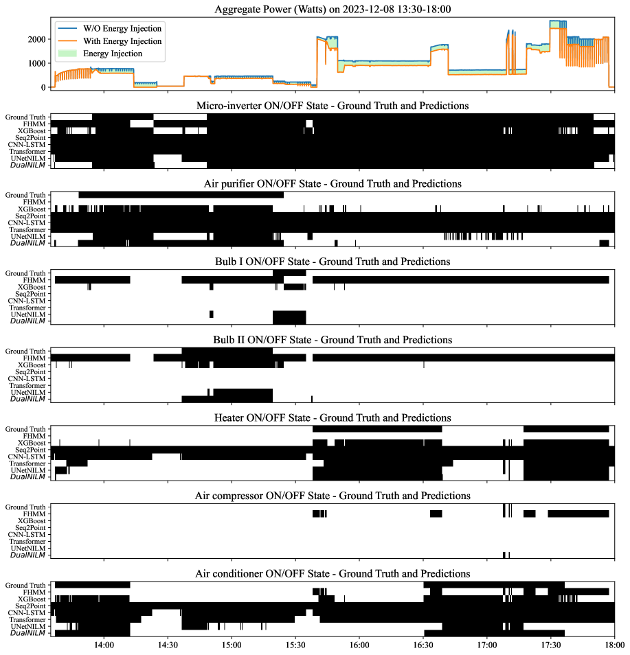
Figure 5: Visualization the Predictions of Appliances State (ON:$\blacksquare$/OFF:$\square$) on Dec.8, 2023 of our dataset

Appendix E More Details of Experiment Result

In this section, we will present the full version of all experiment results on all datasets, including our laboratory dataset and synthetic datasets.

E-A Overview of all Results Cross all Dataset

TableVII and VIII show the overall average performance metrics on appliance state recognization and energy injection disaggregation tasks.

TABLE VII: Overall Avg. Performance Metrics (Cross-validation on all splits of each Dataset)

Dataset		Method	Accuracy (%)	Recall (%)	Precision (%)	F1 (%)
Laboratory Dataset (Real Behind-the-Meter Injection)		FHMM	60.95${}_{\scriptstyle\,\pm 27.96}$	28.32${}_{\scriptstyle\,\pm 40.81}$	16.84${}_{\scriptstyle\,\pm 28.20}$	17.25${}_{\scriptstyle\,\pm 27.23}$
		XGBoost	85.82${}_{\scriptstyle\,\pm 2.07}$	48.20${}_{\scriptstyle\,\pm 7.69}$	52.10${}_{\scriptstyle\,\pm 6.02}$	47.75${}_{\scriptstyle\,\pm 6.75}$
		Seq2Point	67.63${}_{\scriptstyle\,\pm 17.08}$	53.06${}_{\scriptstyle\,\pm 10.80}$	27.86${}_{\scriptstyle\,\pm 14.16}$	34.27${}_{\scriptstyle\,\pm 13.29}$
		CNN-LSTM	74.03${}_{\scriptstyle\,\pm 15.51}$	52.97${}_{\scriptstyle\,\pm 11.02}$	30.29${}_{\scriptstyle\,\pm 14.28}$	36.67${}_{\scriptstyle\,\pm 13.25}$
		Transformer	81.79${}_{\scriptstyle\,\pm 12.65}$	52.91${}_{\scriptstyle\,\pm 10.76}$	38.16${}_{\scriptstyle\,\pm 15.53}$	42.76${}_{\scriptstyle\,\pm 14.02}$
		UNetNILM	89.20${}_{\scriptstyle\,\pm 9.76}$	54.01${}_{\scriptstyle\,\pm 27.35}$	60.81${}_{\scriptstyle\,\pm 30.96}$	53.89${}_{\scriptstyle\,\pm 27.00}$
		DualNILM	98.54${}_{\scriptstyle\,\pm 1.71}$	85.43${}_{\scriptstyle\,\pm 28.03}$	84.16${}_{\scriptstyle\,\pm 28.45}$	84.54${}_{\scriptstyle\,\pm 27.93}$
REDD (Synthetic PV Injection)	House 1	FHMM	79.52${}_{\scriptstyle\,\pm 39.21}$	1.46${}_{\scriptstyle\,\pm 3.60}$	13.47${}_{\scriptstyle\,\pm 33.46}$	2.07${}_{\scriptstyle\,\pm 6.20}$
		XGBoost	97.90${}_{\scriptstyle\,\pm 0.38}$	74.50${}_{\scriptstyle\,\pm 2.64}$	88.74${}_{\scriptstyle\,\pm 2.08}$	79.18${}_{\scriptstyle\,\pm 1.79}$
		Seq2Point	97.65${}_{\scriptstyle\,\pm 0.46}$	42.20${}_{\scriptstyle\,\pm 3.43}$	56.42${}_{\scriptstyle\,\pm 1.16}$	46.07${}_{\scriptstyle\,\pm 4.03}$
		CNN-LSTM	98.67${}_{\scriptstyle\,\pm 0.46}$	46.32${}_{\scriptstyle\,\pm 2.41}$	50.75${}_{\scriptstyle\,\pm 3.19}$	47.96${}_{\scriptstyle\,\pm 2.07}$
		Transformer	95.99${}_{\scriptstyle\,\pm 1.10}$	56.08${}_{\scriptstyle\,\pm 5.37}$	54.10${}_{\scriptstyle\,\pm 8.04}$	53.42${}_{\scriptstyle\,\pm 6.31}$
		UNetNILM	99.05${}_{\scriptstyle\,\pm 0.31}$	76.11${}_{\scriptstyle\,\pm 3.42}$	85.22${}_{\scriptstyle\,\pm 5.99}$	75.27${}_{\scriptstyle\,\pm 4.25}$
		DualNILM	99.84${}_{\scriptstyle\,\pm 0.07}$	96.26${}_{\scriptstyle\,\pm 3.15}$	97.11${}_{\scriptstyle\,\pm 1.90}$	96.64${}_{\scriptstyle\,\pm 2.42}$
	House 2	FHMM	75.08${}_{\scriptstyle\,\pm 42.51}$	0.58${}_{\scriptstyle\,\pm 1.35}$	0.34${}_{\scriptstyle\,\pm 0.79}$	0.43${}_{\scriptstyle\,\pm 1.00}$
		XGBoost	98.43${}_{\scriptstyle\,\pm 0.09}$	92.47${}_{\scriptstyle\,\pm 3.94}$	95.58${}_{\scriptstyle\,\pm 1.21}$	93.53${}_{\scriptstyle\,\pm 3.15}$
		Seq2Point	91.43${}_{\scriptstyle\,\pm 1.50}$	52.90${}_{\scriptstyle\,\pm 2.47}$	58.44${}_{\scriptstyle\,\pm 1.59}$	50.85${}_{\scriptstyle\,\pm 2.27}$
		CNN-LSTM	98.86${}_{\scriptstyle\,\pm 0.32}$	49.19${}_{\scriptstyle\,\pm 0.39}$	48.74${}_{\scriptstyle\,\pm 0.15}$	48.96${}_{\scriptstyle\,\pm 0.26}$
		Transformer	97.92${}_{\scriptstyle\,\pm 0.19}$	47.78${}_{\scriptstyle\,\pm 0.35}$	47.98${}_{\scriptstyle\,\pm 0.50}$	47.87${}_{\scriptstyle\,\pm 0.22}$
		UNetNILM	99.57${}_{\scriptstyle\,\pm 0.22}$	64.16${}_{\scriptstyle\,\pm 16.03}$	77.22${}_{\scriptstyle\,\pm 20.61}$	67.28${}_{\scriptstyle\,\pm 17.02}$
		DualNILM	99.70${}_{\scriptstyle\,\pm 0.22}$	92.48${}_{\scriptstyle\,\pm 5.55}$	94.00${}_{\scriptstyle\,\pm 5.47}$	93.11${}_{\scriptstyle\,\pm 4.96}$
	House 3	FHMM	83.84${}_{\scriptstyle\,\pm 27.80}$	4.53${}_{\scriptstyle\,\pm 8.79}$	0.90${}_{\scriptstyle\,\pm 1.69}$	1.49${}_{\scriptstyle\,\pm 2.80}$
		XGBoost	94.89${}_{\scriptstyle\,\pm 2.15}$	46.22${}_{\scriptstyle\,\pm 0.48}$	56.38${}_{\scriptstyle\,\pm 2.49}$	50.51${}_{\scriptstyle\,\pm 1.28}$
		Seq2Point	98.10${}_{\scriptstyle\,\pm 0.88}$	42.78${}_{\scriptstyle\,\pm 7.36}$	50.90${}_{\scriptstyle\,\pm 11.98}$	44.47${}_{\scriptstyle\,\pm 7.97}$
		CNN-LSTM	95.92${}_{\scriptstyle\,\pm 2.70}$	28.85${}_{\scriptstyle\,\pm 5.34}$	38.17${}_{\scriptstyle\,\pm 0.75}$	32.62${}_{\scriptstyle\,\pm 3.48}$
		Transformer	97.81${}_{\scriptstyle\,\pm 0.61}$	40.21${}_{\scriptstyle\,\pm 5.32}$	38.89${}_{\scriptstyle\,\pm 4.60}$	39.43${}_{\scriptstyle\,\pm 4.67}$
		UNetNILM	99.07${}_{\scriptstyle\,\pm 0.32}$	59.91${}_{\scriptstyle\,\pm 0.04}$	54.73${}_{\scriptstyle\,\pm 1.56}$	57.10${}_{\scriptstyle\,\pm 0.95}$
		DualNILM	99.69${}_{\scriptstyle\,\pm 0.24}$	77.42${}_{\scriptstyle\,\pm 17.13}$	84.46${}_{\scriptstyle\,\pm 12.18}$	80.04${}_{\scriptstyle\,\pm 15.51}$
UKDALE (Synthetic PV Injection)	House 1	FHMM	89.25${}_{\scriptstyle\,\pm 23.05}$	1.58${}_{\scriptstyle\,\pm 3.57}$	0.76${}_{\scriptstyle\,\pm 1.87}$	1.01${}_{\scriptstyle\,\pm 2.39}$
		XGBoost	93.64${}_{\scriptstyle\,\pm 0.42}$	41.74${}_{\scriptstyle\,\pm 1.40}$	68.04${}_{\scriptstyle\,\pm 3.98}$	45.97${}_{\scriptstyle\,\pm 2.56}$
		Seq2Point	88.70${}_{\scriptstyle\,\pm 0.58}$	41.47${}_{\scriptstyle\,\pm 2.83}$	43.29${}_{\scriptstyle\,\pm 5.22}$	36.79${}_{\scriptstyle\,\pm 3.32}$
		CNN-LSTM	98.33${}_{\scriptstyle\,\pm 0.24}$	31.76${}_{\scriptstyle\,\pm 0.20}$	31.29${}_{\scriptstyle\,\pm 0.24}$	31.52${}_{\scriptstyle\,\pm 0.15}$
		Transformer	96.90${}_{\scriptstyle\,\pm 0.29}$	33.65${}_{\scriptstyle\,\pm 1.03}$	27.76${}_{\scriptstyle\,\pm 2.49}$	30.26${}_{\scriptstyle\,\pm 1.69}$
		UNetNILM	98.76${}_{\scriptstyle\,\pm 0.16}$	52.03${}_{\scriptstyle\,\pm 5.14}$	72.01${}_{\scriptstyle\,\pm 18.92}$	55.20${}_{\scriptstyle\,\pm 7.02}$
		DualNILM	99.72${}_{\scriptstyle\,\pm 0.21}$	95.23${}_{\scriptstyle\,\pm 3.53}$	94.30${}_{\scriptstyle\,\pm 4.09}$	94.71${}_{\scriptstyle\,\pm 3.63}$
	House 2	FHMM	82.95${}_{\scriptstyle\,\pm 36.49}$	0.62${}_{\scriptstyle\,\pm 1.17}$	0.52${}_{\scriptstyle\,\pm 1.01}$	0.55${}_{\scriptstyle\,\pm 1.06}$
		XGBoost	96.13${}_{\scriptstyle\,\pm 0.61}$	66.61${}_{\scriptstyle\,\pm 5.32}$	79.19${}_{\scriptstyle\,\pm 9.68}$	70.67${}_{\scriptstyle\,\pm 6.81}$
		Seq2Point	98.83${}_{\scriptstyle\,\pm 0.18}$	42.68${}_{\scriptstyle\,\pm 3.09}$	46.49${}_{\scriptstyle\,\pm 12.53}$	41.92${}_{\scriptstyle\,\pm 3.19}$
		CNN-LSTM	97.81${}_{\scriptstyle\,\pm 0.86}$	41.65${}_{\scriptstyle\,\pm 5.05}$	45.48${}_{\scriptstyle\,\pm 3.20}$	43.33${}_{\scriptstyle\,\pm 4.21}$
		Transformer	99.13${}_{\scriptstyle\,\pm 0.14}$	59.88${}_{\scriptstyle\,\pm 5.10}$	77.44${}_{\scriptstyle\,\pm 7.86}$	61.73${}_{\scriptstyle\,\pm 4.66}$
		UNetNILM	99.17${}_{\scriptstyle\,\pm 0.19}$	64.25${}_{\scriptstyle\,\pm 5.53}$	68.74${}_{\scriptstyle\,\pm 5.74}$	65.43${}_{\scriptstyle\,\pm 4.72}$
		DualNILM	99.73${}_{\scriptstyle\,\pm 0.04}$	90.63${}_{\scriptstyle\,\pm 5.01}$	94.46${}_{\scriptstyle\,\pm 3.36}$	92.31${}_{\scriptstyle\,\pm 3.76}$

TABLE VIII: Overall Avg. Performance Metrics of Energy Injection Disaggregation (Cross-validation on all splits of each Dataset)

Dataset		Method	Avg. RMSE	Avg. MAE
Laboratory Dataset (Real Behind-the-Meter Injection)		FHMM	0.5015${}_{\scriptstyle\,\pm 0.0823}$	0.4492${}_{\scriptstyle\,\pm 0.0867}$
		Seq2Seq	0.3512${}_{\scriptstyle\,\pm 0.1111}$	0.2622${}_{\scriptstyle\,\pm 0.0888}$
		DAE	0.8830${}_{\scriptstyle\,\pm 0.0803}$	0.7851${}_{\scriptstyle\,\pm 0.1410}$
		UNetNILM	0.2305${}_{\scriptstyle\,\pm 0.0858}$	0.1883${}_{\scriptstyle\,\pm 0.0802}$
		DualNILM	0.1429${}_{\scriptstyle\,\pm 0.0896}$	0.0804${}_{\scriptstyle\,\pm 0.0677}$
REDD (Synthetic PV Injection)	House 1	FHMM	0.8093${}_{\scriptstyle\,\pm 0.0141}$	0.2200${}_{\scriptstyle\,\pm 0.0054}$
		Seq2Seq	0.6834${}_{\scriptstyle\,\pm 0.0217}$	0.2370${}_{\scriptstyle\,\pm 0.0121}$
		DAE	0.8115${}_{\scriptstyle\,\pm 0.0172}$	0.2171${}_{\scriptstyle\,\pm 0.0069}$
		UNetNILM	0.7589${}_{\scriptstyle\,\pm 0.1951}$	0.1983${}_{\scriptstyle\,\pm 0.0164}$
		DualNILM	0.6661${}_{\scriptstyle\,\pm 0.0145}$	0.1777${}_{\scriptstyle\,\pm 0.0056}$
	House 2	FHMM	0.8403${}_{\scriptstyle\,\pm 0.1384}$	0.3367${}_{\scriptstyle\,\pm 0.0629}$
		Seq2Seq	0.7217${}_{\scriptstyle\,\pm 0.1521}$	0.3287${}_{\scriptstyle\,\pm 0.0624}$
		DAE	0.8448${}_{\scriptstyle\,\pm 0.1703}$	0.3356${}_{\scriptstyle\,\pm 0.0782}$
		UNetNILM	2.2077${}_{\scriptstyle\,\pm 0.6670}$	0.6601${}_{\scriptstyle\,\pm 0.1903}$
		DualNILM	0.7065${}_{\scriptstyle\,\pm 0.1419}$	0.2768${}_{\scriptstyle\,\pm 0.0648}$
	House 3	FHMM	0.5575${}_{\scriptstyle\,\pm 0.0574}$	0.1766${}_{\scriptstyle\,\pm 0.0532}$
		Seq2Seq	0.4974${}_{\scriptstyle\,\pm 0.0543}$	0.1940${}_{\scriptstyle\,\pm 0.0505}$
		DAE	0.5606${}_{\scriptstyle\,\pm 0.0704}$	0.1743${}_{\scriptstyle\,\pm 0.0660}$
		UNetNILM	2.2517${}_{\scriptstyle\,\pm 0.2121}$	0.4708${}_{\scriptstyle\,\pm 0.1640}$
		DualNILM	0.4261${}_{\scriptstyle\,\pm 0.0582}$	0.1422${}_{\scriptstyle\,\pm 0.0546}$
UKDALE (Synthetic PV Injection)	House 1	FHMM	1.1905${}_{\scriptstyle\,\pm 0.0936}$	0.3331${}_{\scriptstyle\,\pm 0.0015}$
		Seq2Seq	0.9055${}_{\scriptstyle\,\pm 0.0211}$	0.2758${}_{\scriptstyle\,\pm 0.0103}$
		DAE	0.9197${}_{\scriptstyle\,\pm 0.0255}$	0.2948${}_{\scriptstyle\,\pm 0.0128}$
		UNetNILM	7.5014${}_{\scriptstyle\,\pm 0.5703}$	1.3871${}_{\scriptstyle\,\pm 0.1633}$
		DualNILM	0.9008${}_{\scriptstyle\,\pm 0.0957}$	0.2731${}_{\scriptstyle\,\pm 0.0020}$
	House 2	FHMM	1.1477${}_{\scriptstyle\,\pm 0.0213}$	0.3521${}_{\scriptstyle\,\pm 0.0101}$
		Seq2Seq	0.9252${}_{\scriptstyle\,\pm 0.0256}$	0.2833${}_{\scriptstyle\,\pm 0.0165}$
		DAE	0.9594${}_{\scriptstyle\,\pm 0.0309}$	0.3368${}_{\scriptstyle\,\pm 0.0202}$
		UNetNILM	1.1285${}_{\scriptstyle\,\pm 0.0022}$	0.3043${}_{\scriptstyle\,\pm 0.0046}$
		DualNILM	0.9344${}_{\scriptstyle\,\pm 0.0216}$	0.2883${}_{\scriptstyle\,\pm 0.0103}$

E-B Laboratory Dataset Results

Table. IX shows the details of the laboratory dataset performance metrics for DualNILM and benchmarks.

Fig. 5 shows all seven different appliances (including micro-inverter)’s ground truth state, DualNILM, and benchmarks prediction on Dec.8, 2023 of our dataset.

TABLE IX: Laboratory Dataset Performance Metrics (cross-validation on all dates)

Appliance	Method	Accuracy (%)	Recall (%)	Precision (%)	F1 (%)
Air compressor	FHMM	99.56${}_{\scriptstyle\,\pm 0.20}$	14.29${}_{\scriptstyle\,\pm 34.99}$	14.29${}_{\scriptstyle\,\pm 34.99}$	14.29${}_{\scriptstyle\,\pm 34.99}$
	XGBoost	99.55${}_{\scriptstyle\,\pm 0.23}$	0.00${}_{\scriptstyle\,\pm 0.00}$	0.00${}_{\scriptstyle\,\pm 0.00}$	0.00${}_{\scriptstyle\,\pm 0.00}$
	Seq2Point	99.52${}_{\scriptstyle\,\pm 0.25}$	0.00${}_{\scriptstyle\,\pm 0.00}$	0.00${}_{\scriptstyle\,\pm 0.00}$	0.00${}_{\scriptstyle\,\pm 0.00}$
	CNN-LSTM	99.52${}_{\scriptstyle\,\pm 0.25}$	0.00${}_{\scriptstyle\,\pm 0.00}$	0.00${}_{\scriptstyle\,\pm 0.00}$	0.00${}_{\scriptstyle\,\pm 0.00}$
	Transformer	99.52${}_{\scriptstyle\,\pm 0.25}$	0.00${}_{\scriptstyle\,\pm 0.00}$	0.00${}_{\scriptstyle\,\pm 0.00}$	0.00${}_{\scriptstyle\,\pm 0.00}$
	UNetNILM	99.52${}_{\scriptstyle\,\pm 0.25}$	0.00${}_{\scriptstyle\,\pm 0.00}$	0.00${}_{\scriptstyle\,\pm 0.00}$	0.00${}_{\scriptstyle\,\pm 0.00}$
	DualNILM	99.97${}_{\scriptstyle\,\pm 0.03}$	83.77${}_{\scriptstyle\,\pm 37.10}$	83.40${}_{\scriptstyle\,\pm 36.97}$	83.52${}_{\scriptstyle\,\pm 36.91}$
Air conditioner	FHMM	60.46${}_{\scriptstyle\,\pm 24.50}$	0.06${}_{\scriptstyle\,\pm 0.14}$	14.29${}_{\scriptstyle\,\pm 34.99}$	0.11${}_{\scriptstyle\,\pm 0.28}$
	XGBoost	85.28${}_{\scriptstyle\,\pm 8.06}$	79.10${}_{\scriptstyle\,\pm 21.44}$	78.25${}_{\scriptstyle\,\pm 21.04}$	77.24${}_{\scriptstyle\,\pm 18.25}$
	Seq2Point	41.63${}_{\scriptstyle\,\pm 26.47}$	100.00${}_{\scriptstyle\,\pm 0.00}$	41.63${}_{\scriptstyle\,\pm 26.47}$	55.46${}_{\scriptstyle\,\pm 20.96}$
	CNN-LSTM	63.85${}_{\scriptstyle\,\pm 21.92}$	99.40${}_{\scriptstyle\,\pm 1.59}$	52.71${}_{\scriptstyle\,\pm 24.63}$	66.29${}_{\scriptstyle\,\pm 18.88}$
	Transformer	73.70${}_{\scriptstyle\,\pm 21.33}$	99.92${}_{\scriptstyle\,\pm 0.10}$	61.77${}_{\scriptstyle\,\pm 26.68}$	73.58${}_{\scriptstyle\,\pm 19.57}$
	UNetNILM	84.72${}_{\scriptstyle\,\pm 13.12}$	68.70${}_{\scriptstyle\,\pm 38.16}$	71.17${}_{\scriptstyle\,\pm 37.78}$	69.50${}_{\scriptstyle\,\pm 37.22}$
	DualNILM	99.57${}_{\scriptstyle\,\pm 0.74}$	99.41${}_{\scriptstyle\,\pm 0.89}$	98.94${}_{\scriptstyle\,\pm 2.45}$	99.17${}_{\scriptstyle\,\pm 1.61}$
Air purifier	FHMM	36.96${}_{\scriptstyle\,\pm 12.04}$	48.72${}_{\scriptstyle\,\pm 30.24}$	36.41${}_{\scriptstyle\,\pm 26.63}$	36.37${}_{\scriptstyle\,\pm 20.83}$
	XGBoost	58.30${}_{\scriptstyle\,\pm 10.43}$	44.27${}_{\scriptstyle\,\pm 29.30}$	45.73${}_{\scriptstyle\,\pm 26.07}$	40.50${}_{\scriptstyle\,\pm 21.78}$
	Seq2Point	42.71${}_{\scriptstyle\,\pm 30.69}$	85.71${}_{\scriptstyle\,\pm 37.80}$	42.71${}_{\scriptstyle\,\pm 30.69}$	53.99${}_{\scriptstyle\,\pm 32.38}$
	CNN-LSTM	42.71${}_{\scriptstyle\,\pm 30.69}$	85.71${}_{\scriptstyle\,\pm 37.80}$	42.71${}_{\scriptstyle\,\pm 30.69}$	53.99${}_{\scriptstyle\,\pm 32.38}$
	Transformer	42.71${}_{\scriptstyle\,\pm 30.69}$	85.71${}_{\scriptstyle\,\pm 37.80}$	42.71${}_{\scriptstyle\,\pm 30.69}$	53.99${}_{\scriptstyle\,\pm 32.38}$
	UNetNILM	74.15${}_{\scriptstyle\,\pm 22.59}$	60.96${}_{\scriptstyle\,\pm 38.01}$	66.36${}_{\scriptstyle\,\pm 31.88}$	60.32${}_{\scriptstyle\,\pm 31.63}$
	DualNILM	93.58${}_{\scriptstyle\,\pm 6.52}$	81.38${}_{\scriptstyle\,\pm 36.60}$	80.01${}_{\scriptstyle\,\pm 36.09}$	80.38${}_{\scriptstyle\,\pm 35.81}$
Heater	FHMM	54.31${}_{\scriptstyle\,\pm 21.71}$	85.71${}_{\scriptstyle\,\pm 34.99}$	37.34${}_{\scriptstyle\,\pm 28.83}$	48.05${}_{\scriptstyle\,\pm 30.75}$
	XGBoost	95.37${}_{\scriptstyle\,\pm 3.89}$	81.65${}_{\scriptstyle\,\pm 36.30}$	80.21${}_{\scriptstyle\,\pm 36.74}$	80.51${}_{\scriptstyle\,\pm 35.85}$
	Seq2Point	31.97${}_{\scriptstyle\,\pm 27.87}$	85.71${}_{\scriptstyle\,\pm 37.80}$	31.97${}_{\scriptstyle\,\pm 27.87}$	43.00${}_{\scriptstyle\,\pm 30.73}$
	CNN-LSTM	54.57${}_{\scriptstyle\,\pm 21.39}$	85.65${}_{\scriptstyle\,\pm 37.77}$	37.94${}_{\scriptstyle\,\pm 30.61}$	48.92${}_{\scriptstyle\,\pm 32.57}$
	Transformer	99.01${}_{\scriptstyle\,\pm 1.95}$	84.77${}_{\scriptstyle\,\pm 37.44}$	83.94${}_{\scriptstyle\,\pm 37.28}$	84.29${}_{\scriptstyle\,\pm 37.24}$
	UNetNILM	98.33${}_{\scriptstyle\,\pm 3.80}$	82.59${}_{\scriptstyle\,\pm 37.28}$	85.00${}_{\scriptstyle\,\pm 37.49}$	83.62${}_{\scriptstyle\,\pm 37.14}$
	DualNILM	98.77${}_{\scriptstyle\,\pm 1.95}$	84.88${}_{\scriptstyle\,\pm 37.47}$	79.08${}_{\scriptstyle\,\pm 38.35}$	81.11${}_{\scriptstyle\,\pm 37.16}$
Light bulb Type I	FHMM	74.81${}_{\scriptstyle\,\pm 14.33}$	0.00${}_{\scriptstyle\,\pm 0.00}$	0.00${}_{\scriptstyle\,\pm 0.00}$	0.00${}_{\scriptstyle\,\pm 0.00}$
	XGBoost	87.75${}_{\scriptstyle\,\pm 9.90}$	4.26${}_{\scriptstyle\,\pm 7.87}$	23.20${}_{\scriptstyle\,\pm 36.84}$	6.88${}_{\scriptstyle\,\pm 12.93}$
	Seq2Point	88.53${}_{\scriptstyle\,\pm 12.75}$	0.00${}_{\scriptstyle\,\pm 0.00}$	0.00${}_{\scriptstyle\,\pm 0.00}$	0.00${}_{\scriptstyle\,\pm 0.00}$
	CNN-LSTM	88.53${}_{\scriptstyle\,\pm 12.75}$	0.00${}_{\scriptstyle\,\pm 0.00}$	0.00${}_{\scriptstyle\,\pm 0.00}$	0.00${}_{\scriptstyle\,\pm 0.00}$
	Transformer	88.53${}_{\scriptstyle\,\pm 12.75}$	0.00${}_{\scriptstyle\,\pm 0.00}$	0.00${}_{\scriptstyle\,\pm 0.00}$	0.00${}_{\scriptstyle\,\pm 0.00}$
	UNetNILM	89.83${}_{\scriptstyle\,\pm 11.82}$	16.59${}_{\scriptstyle\,\pm 35.97}$	51.65${}_{\scriptstyle\,\pm 49.12}$	17.93${}_{\scriptstyle\,\pm 34.46}$
	DualNILM	99.63${}_{\scriptstyle\,\pm 0.57}$	67.66${}_{\scriptstyle\,\pm 46.76}$	64.40${}_{\scriptstyle\,\pm 47.41}$	65.59${}_{\scriptstyle\,\pm 46.77}$
Light bulb Type II	FHMM	74.81${}_{\scriptstyle\,\pm 14.33}$	0.00${}_{\scriptstyle\,\pm 0.00}$	0.00${}_{\scriptstyle\,\pm 0.00}$	0.00${}_{\scriptstyle\,\pm 0.00}$
	XGBoost	91.48${}_{\scriptstyle\,\pm 7.08}$	39.80${}_{\scriptstyle\,\pm 41.77}$	48.57${}_{\scriptstyle\,\pm 37.99}$	41.06${}_{\scriptstyle\,\pm 37.49}$
	Seq2Point	90.35${}_{\scriptstyle\,\pm 7.49}$	0.00${}_{\scriptstyle\,\pm 0.00}$	0.00${}_{\scriptstyle\,\pm 0.00}$	0.00${}_{\scriptstyle\,\pm 0.00}$
	CNN-LSTM	90.35${}_{\scriptstyle\,\pm 7.49}$	0.00${}_{\scriptstyle\,\pm 0.00}$	0.00${}_{\scriptstyle\,\pm 0.00}$	0.00${}_{\scriptstyle\,\pm 0.00}$
	Transformer	90.35${}_{\scriptstyle\,\pm 7.49}$	0.00${}_{\scriptstyle\,\pm 0.00}$	0.00${}_{\scriptstyle\,\pm 0.00}$	0.00${}_{\scriptstyle\,\pm 0.00}$
	UNetNILM	94.97${}_{\scriptstyle\,\pm 4.49}$	50.57${}_{\scriptstyle\,\pm 40.13}$	68.62${}_{\scriptstyle\,\pm 47.29}$	56.37${}_{\scriptstyle\,\pm 40.50}$
	DualNILM	99.05${}_{\scriptstyle\,\pm 1.33}$	81.57${}_{\scriptstyle\,\pm 36.42}$	83.89${}_{\scriptstyle\,\pm 37.05}$	82.63${}_{\scriptstyle\,\pm 36.59}$
Micro-inverter	FHMM	25.73${}_{\scriptstyle\,\pm 10.43}$	49.49${}_{\scriptstyle\,\pm 39.18}$	15.59${}_{\scriptstyle\,\pm 13.83}$	21.93${}_{\scriptstyle\,\pm 18.81}$
	XGBoost	83.04${}_{\scriptstyle\,\pm 13.23}$	88.33${}_{\scriptstyle\,\pm 9.13}$	88.75${}_{\scriptstyle\,\pm 12.75}$	88.09${}_{\scriptstyle\,\pm 9.65}$
	Seq2Point	78.68${}_{\scriptstyle\,\pm 14.06}$	100.00${}_{\scriptstyle\,\pm 0.00}$	78.68${}_{\scriptstyle\,\pm 14.06}$	87.46${}_{\scriptstyle\,\pm 8.93}$
	CNN-LSTM	78.68${}_{\scriptstyle\,\pm 14.06}$	100.00${}_{\scriptstyle\,\pm 0.00}$	78.68${}_{\scriptstyle\,\pm 14.06}$	87.46${}_{\scriptstyle\,\pm 8.93}$
	Transformer	78.68${}_{\scriptstyle\,\pm 14.06}$	100.00${}_{\scriptstyle\,\pm 0.00}$	78.68${}_{\scriptstyle\,\pm 14.06}$	87.46${}_{\scriptstyle\,\pm 8.93}$
	UNetNILM	82.85${}_{\scriptstyle\,\pm 12.23}$	98.64${}_{\scriptstyle\,\pm 1.91}$	82.87${}_{\scriptstyle\,\pm 13.19}$	89.48${}_{\scriptstyle\,\pm 8.09}$
	DualNILM	99.17${}_{\scriptstyle\,\pm 0.81}$	99.37${}_{\scriptstyle\,\pm 0.93}$	99.42${}_{\scriptstyle\,\pm 0.80}$	99.39${}_{\scriptstyle\,\pm 0.63}$
Avg.	FHMM	60.95${}_{\scriptstyle\,\pm 27.96}$	28.32${}_{\scriptstyle\,\pm 40.81}$	16.84${}_{\scriptstyle\,\pm 28.20}$	17.25${}_{\scriptstyle\,\pm 27.23}$
	XGBoost	85.82${}_{\scriptstyle\,\pm 2.07}$	48.20${}_{\scriptstyle\,\pm 7.69}$	52.10${}_{\scriptstyle\,\pm 6.02}$	47.75${}_{\scriptstyle\,\pm 6.75}$
	Seq2Point	67.63${}_{\scriptstyle\,\pm 17.08}$	53.06${}_{\scriptstyle\,\pm 10.80}$	27.86${}_{\scriptstyle\,\pm 14.16}$	34.27${}_{\scriptstyle\,\pm 13.29}$
	CNN-LSTM	74.03${}_{\scriptstyle\,\pm 15.51}$	52.97${}_{\scriptstyle\,\pm 11.02}$	30.29${}_{\scriptstyle\,\pm 14.28}$	36.67${}_{\scriptstyle\,\pm 13.25}$
	Transformer	81.79${}_{\scriptstyle\,\pm 12.65}$	52.91${}_{\scriptstyle\,\pm 10.76}$	38.16${}_{\scriptstyle\,\pm 15.53}$	42.76${}_{\scriptstyle\,\pm 14.02}$
	UNetNILM	89.20${}_{\scriptstyle\,\pm 9.76}$	54.01${}_{\scriptstyle\,\pm 27.35}$	60.81${}_{\scriptstyle\,\pm 30.96}$	53.89${}_{\scriptstyle\,\pm 27.00}$
	DualNILM	98.54${}_{\scriptstyle\,\pm 1.71}$	85.43${}_{\scriptstyle\,\pm 28.03}$	84.16${}_{\scriptstyle\,\pm 28.45}$	84.54${}_{\scriptstyle\,\pm 27.93}$
Injection Disaggregation	FHMM	Avg. RMSE: 0.5015${}_{\scriptstyle\,\pm 0.0823}$		Avg. MAE: 0.4492${}_{\scriptstyle\,\pm 0.0867}$
	Seq2Seq	Avg. RMSE: 0.3512${}_{\scriptstyle\,\pm 0.1111}$		Avg. MAE: 0.2622${}_{\scriptstyle\,\pm 0.0888}$
	DAE	Avg. RMSE: 0.8830${}_{\scriptstyle\,\pm 0.0803}$		Avg. MAE: 0.7851${}_{\scriptstyle\,\pm 0.1410}$
	UNetNILM	Avg. RMSE: 0.2305${}_{\scriptstyle\,\pm 0.0858}$		Avg. MAE: 0.1883${}_{\scriptstyle\,\pm 0.0802}$
	DualNILM	Avg. RMSE: 0.1429${}_{\scriptstyle\,\pm 0.0896}$		Avg. MAE: 0.0804${}_{\scriptstyle\,\pm 0.0677}$

E-C REDD Dataset Results

E-C1 Full Results on House 1

See Table X.

TABLE X: REDD House 1 Performance Metrics (cross-validation on all splits)

Appliance	Method	Accuracy (%)	Recall (%)	Precision (%)	F1 (%)
Microwave	FHMM	99.13${}_{\scriptstyle\,\pm 0.53}$	0.06${}_{\scriptstyle\,\pm 0.09}$	33.33${}_{\scriptstyle\,\pm 47.14}$	0.12${}_{\scriptstyle\,\pm 0.17}$
	XGBoost	99.40${}_{\scriptstyle\,\pm 0.32}$	44.51${}_{\scriptstyle\,\pm 21.18}$	72.75${}_{\scriptstyle\,\pm 8.68}$	52.40${}_{\scriptstyle\,\pm 17.83}$
	Seq2Point	99.37${}_{\scriptstyle\,\pm 0.60}$	35.85${}_{\scriptstyle\,\pm 15.53}$	98.67${}_{\scriptstyle\,\pm 0.41}$	51.25${}_{\scriptstyle\,\pm 17.22}$
	CNN-LSTM	99.11${}_{\scriptstyle\,\pm 0.66}$	0.00${}_{\scriptstyle\,\pm 0.00}$	0.00${}_{\scriptstyle\,\pm 0.00}$	0.00${}_{\scriptstyle\,\pm 0.00}$
	Transformer	99.11${}_{\scriptstyle\,\pm 0.66}$	0.00${}_{\scriptstyle\,\pm 0.00}$	0.00${}_{\scriptstyle\,\pm 0.00}$	0.00${}_{\scriptstyle\,\pm 0.00}$
	UNetNILM	99.22${}_{\scriptstyle\,\pm 0.63}$	20.76${}_{\scriptstyle\,\pm 10.51}$	84.45${}_{\scriptstyle\,\pm 15.52}$	31.96${}_{\scriptstyle\,\pm 14.16}$
	DualNILM	99.90${}_{\scriptstyle\,\pm 0.07}$	88.10${}_{\scriptstyle\,\pm 10.07}$	95.87${}_{\scriptstyle\,\pm 5.23}$	91.75${}_{\scriptstyle\,\pm 7.75}$
Fridge	FHMM	99.96${}_{\scriptstyle\,\pm 0.02}$	0.00${}_{\scriptstyle\,\pm 0.00}$	0.00${}_{\scriptstyle\,\pm 0.00}$	0.00${}_{\scriptstyle\,\pm 0.00}$
	XGBoost	91.91${}_{\scriptstyle\,\pm 1.33}$	59.20${}_{\scriptstyle\,\pm 5.63}$	91.80${}_{\scriptstyle\,\pm 2.41}$	71.92${}_{\scriptstyle\,\pm 4.81}$
	Seq2Point	93.99${}_{\scriptstyle\,\pm 0.98}$	80.91${}_{\scriptstyle\,\pm 0.46}$	84.44${}_{\scriptstyle\,\pm 5.25}$	82.58${}_{\scriptstyle\,\pm 2.37}$
	CNN-LSTM	97.02${}_{\scriptstyle\,\pm 0.70}$	91.32${}_{\scriptstyle\,\pm 1.50}$	91.93${}_{\scriptstyle\,\pm 1.54}$	91.61${}_{\scriptstyle\,\pm 0.56}$
	Transformer	84.18${}_{\scriptstyle\,\pm 3.66}$	78.06${}_{\scriptstyle\,\pm 3.21}$	53.95${}_{\scriptstyle\,\pm 4.15}$	63.72${}_{\scriptstyle\,\pm 3.14}$
	UNetNILM	97.52${}_{\scriptstyle\,\pm 0.45}$	89.83${}_{\scriptstyle\,\pm 1.18}$	95.82${}_{\scriptstyle\,\pm 0.99}$	92.73${}_{\scriptstyle\,\pm 1.09}$
	DualNILM	99.63${}_{\scriptstyle\,\pm 0.13}$	99.49${}_{\scriptstyle\,\pm 0.59}$	98.46${}_{\scriptstyle\,\pm 0.24}$	98.97${}_{\scriptstyle\,\pm 0.33}$
Dish Washer	FHMM	98.64${}_{\scriptstyle\,\pm 0.34}$	4.80${}_{\scriptstyle\,\pm 6.79}$	32.49${}_{\scriptstyle\,\pm 45.95}$	8.37${}_{\scriptstyle\,\pm 11.83}$
	XGBoost	99.61${}_{\scriptstyle\,\pm 0.25}$	89.32${}_{\scriptstyle\,\pm 17.39}$	82.77${}_{\scriptstyle\,\pm 10.17}$	85.03${}_{\scriptstyle\,\pm 9.91}$
	Seq2Point	98.75${}_{\scriptstyle\,\pm 0.23}$	0.00${}_{\scriptstyle\,\pm 0.00}$	0.00${}_{\scriptstyle\,\pm 0.00}$	0.00${}_{\scriptstyle\,\pm 0.00}$
	CNN-LSTM	98.93${}_{\scriptstyle\,\pm 0.29}$	40.75${}_{\scriptstyle\,\pm 10.08}$	62.29${}_{\scriptstyle\,\pm 14.22}$	48.66${}_{\scriptstyle\,\pm 9.54}$
	Transformer	99.12${}_{\scriptstyle\,\pm 0.58}$	76.22${}_{\scriptstyle\,\pm 11.98}$	65.42${}_{\scriptstyle\,\pm 15.59}$	69.89${}_{\scriptstyle\,\pm 13.03}$
	UNetNILM	99.00${}_{\scriptstyle\,\pm 0.35}$	96.16${}_{\scriptstyle\,\pm 2.64}$	56.51${}_{\scriptstyle\,\pm 5.36}$	71.02${}_{\scriptstyle\,\pm 3.45}$
	DualNILM	99.96${}_{\scriptstyle\,\pm 0.02}$	99.47${}_{\scriptstyle\,\pm 0.77}$	97.33${}_{\scriptstyle\,\pm 1.25}$	98.39${}_{\scriptstyle\,\pm 0.56}$
Washing Machine	FHMM	98.78${}_{\scriptstyle\,\pm 0.30}$	0.00${}_{\scriptstyle\,\pm 0.00}$	0.00${}_{\scriptstyle\,\pm 0.00}$	0.00${}_{\scriptstyle\,\pm 0.00}$
	XGBoost	99.74${}_{\scriptstyle\,\pm 0.14}$	81.06${}_{\scriptstyle\,\pm 15.03}$	97.88${}_{\scriptstyle\,\pm 2.06}$	88.10${}_{\scriptstyle\,\pm 9.32}$
	Seq2Point	98.67${}_{\scriptstyle\,\pm 0.42}$	0.00${}_{\scriptstyle\,\pm 0.00}$	0.00${}_{\scriptstyle\,\pm 0.00}$	0.00${}_{\scriptstyle\,\pm 0.00}$
	CNN-LSTM	98.67${}_{\scriptstyle\,\pm 0.42}$	0.00${}_{\scriptstyle\,\pm 0.00}$	0.00${}_{\scriptstyle\,\pm 0.00}$	0.00${}_{\scriptstyle\,\pm 0.00}$
	Transformer	98.79${}_{\scriptstyle\,\pm 0.13}$	26.20${}_{\scriptstyle\,\pm 11.62}$	54.27${}_{\scriptstyle\,\pm 18.90}$	35.11${}_{\scriptstyle\,\pm 14.56}$
	UNetNILM	99.54${}_{\scriptstyle\,\pm 0.11}$	73.82${}_{\scriptstyle\,\pm 2.72}$	89.40${}_{\scriptstyle\,\pm 8.06}$	80.68${}_{\scriptstyle\,\pm 2.55}$
	DualNILM	99.85${}_{\scriptstyle\,\pm 0.07}$	94.26${}_{\scriptstyle\,\pm 4.32}$	94.23${}_{\scriptstyle\,\pm 2.63}$	94.23${}_{\scriptstyle\,\pm 3.39}$
Micro-inverter	FHMM	1.10${}_{\scriptstyle\,\pm 0.25}$	2.45${}_{\scriptstyle\,\pm 0.37}$	1.52${}_{\scriptstyle\,\pm 0.39}$	1.86${}_{\scriptstyle\,\pm 0.37}$
	XGBoost	98.83${}_{\scriptstyle\,\pm 0.08}$	98.41${}_{\scriptstyle\,\pm 0.82}$	98.51${}_{\scriptstyle\,\pm 0.94}$	98.45${}_{\scriptstyle\,\pm 0.19}$
	Seq2Point	97.46${}_{\scriptstyle\,\pm 0.07}$	94.22${}_{\scriptstyle\,\pm 1.15}$	99.01${}_{\scriptstyle\,\pm 0.13}$	96.55${}_{\scriptstyle\,\pm 0.57}$
	CNN-LSTM	99.63${}_{\scriptstyle\,\pm 0.25}$	99.54${}_{\scriptstyle\,\pm 0.46}$	99.53${}_{\scriptstyle\,\pm 0.17}$	99.54${}_{\scriptstyle\,\pm 0.27}$
	Transformer	98.78${}_{\scriptstyle\,\pm 0.46}$	99.93${}_{\scriptstyle\,\pm 0.02}$	96.86${}_{\scriptstyle\,\pm 1.58}$	98.36${}_{\scriptstyle\,\pm 0.81}$
	UNetNILM	99.96${}_{\scriptstyle\,\pm 0.00}$	99.97${}_{\scriptstyle\,\pm 0.03}$	99.92${}_{\scriptstyle\,\pm 0.03}$	99.95${}_{\scriptstyle\,\pm 0.00}$
	DualNILM	99.87${}_{\scriptstyle\,\pm 0.07}$	100.00${}_{\scriptstyle\,\pm 0.00}$	99.68${}_{\scriptstyle\,\pm 0.16}$	99.84${}_{\scriptstyle\,\pm 0.08}$
Avg.	FHMM	79.52${}_{\scriptstyle\,\pm 39.21}$	1.46${}_{\scriptstyle\,\pm 3.60}$	13.47${}_{\scriptstyle\,\pm 33.46}$	2.07${}_{\scriptstyle\,\pm 6.20}$
	XGBoost	97.90${}_{\scriptstyle\,\pm 0.38}$	74.50${}_{\scriptstyle\,\pm 2.64}$	88.74${}_{\scriptstyle\,\pm 2.08}$	79.18${}_{\scriptstyle\,\pm 1.79}$
	Seq2Point	97.65${}_{\scriptstyle\,\pm 0.46}$	42.20${}_{\scriptstyle\,\pm 3.43}$	56.42${}_{\scriptstyle\,\pm 1.16}$	46.07${}_{\scriptstyle\,\pm 4.03}$
	CNN-LSTM	98.67${}_{\scriptstyle\,\pm 0.46}$	46.32${}_{\scriptstyle\,\pm 2.41}$	50.75${}_{\scriptstyle\,\pm 3.19}$	47.96${}_{\scriptstyle\,\pm 2.07}$
	Transformer	95.99${}_{\scriptstyle\,\pm 1.10}$	56.08${}_{\scriptstyle\,\pm 5.37}$	54.10${}_{\scriptstyle\,\pm 8.04}$	53.42${}_{\scriptstyle\,\pm 6.31}$
	UNetNILM	99.05${}_{\scriptstyle\,\pm 0.31}$	76.11${}_{\scriptstyle\,\pm 3.42}$	85.22${}_{\scriptstyle\,\pm 5.99}$	75.27${}_{\scriptstyle\,\pm 4.25}$
	DualNILM	99.84${}_{\scriptstyle\,\pm 0.07}$	96.26${}_{\scriptstyle\,\pm 3.15}$	97.11${}_{\scriptstyle\,\pm 1.90}$	96.64${}_{\scriptstyle\,\pm 2.42}$
Injection Disaggregation	FHMM	Avg. RMSE: 0.8093${}_{\scriptstyle\,\pm 0.0141}$		Avg. MAE: 0.2200${}_{\scriptstyle\,\pm 0.0054}$
	Seq2Seq	Avg. RMSE: 0.6834${}_{\scriptstyle\,\pm 0.0217}$		Avg. MAE: 0.2370${}_{\scriptstyle\,\pm 0.0121}$
	DAE	Avg. RMSE: 0.8115${}_{\scriptstyle\,\pm 0.0172}$		Avg. MAE: 0.2171${}_{\scriptstyle\,\pm 0.0069}$
	UNetNILM	Avg. RMSE: 0.7589${}_{\scriptstyle\,\pm 0.1951}$		Avg. MAE: 0.1983${}_{\scriptstyle\,\pm 0.0164}$
	DualNILM	Avg. RMSE: 0.6661${}_{\scriptstyle\,\pm 0.0145}$		Avg. MAE: 0.1777${}_{\scriptstyle\,\pm 0.0056}$

E-C2 Full Results on House 2

See Table XI.

TABLE XI: REDD House 2 Performance Metrics (cross-validation on all splits)

Appliance	Method	Accuracy (%)	Recall (%)	Precision (%)	F1 (%)
Microwave	FHMM	99.56${}_{\scriptstyle\,\pm 0.21}$	0.00${}_{\scriptstyle\,\pm 0.00}$	0.00${}_{\scriptstyle\,\pm 0.00}$	0.00${}_{\scriptstyle\,\pm 0.00}$
	XGBoost	99.93${}_{\scriptstyle\,\pm 0.01}$	80.21${}_{\scriptstyle\,\pm 16.43}$	99.08${}_{\scriptstyle\,\pm 0.83}$	87.95${}_{\scriptstyle\,\pm 10.38}$
	Seq2Point	99.51${}_{\scriptstyle\,\pm 0.21}$	91.55${}_{\scriptstyle\,\pm 3.13}$	42.30${}_{\scriptstyle\,\pm 5.03}$	57.73${}_{\scriptstyle\,\pm 4.52}$
	CNN-LSTM	99.63${}_{\scriptstyle\,\pm 0.16}$	0.00${}_{\scriptstyle\,\pm 0.00}$	0.00${}_{\scriptstyle\,\pm 0.00}$	0.00${}_{\scriptstyle\,\pm 0.00}$
	Transformer	99.63${}_{\scriptstyle\,\pm 0.16}$	0.00${}_{\scriptstyle\,\pm 0.00}$	0.00${}_{\scriptstyle\,\pm 0.00}$	0.00${}_{\scriptstyle\,\pm 0.00}$
	UNetNILM	99.70${}_{\scriptstyle\,\pm 0.16}$	24.67${}_{\scriptstyle\,\pm 6.83}$	77.10${}_{\scriptstyle\,\pm 24.08}$	37.26${}_{\scriptstyle\,\pm 10.51}$
	DualNILM	99.91${}_{\scriptstyle\,\pm 0.03}$	79.18${}_{\scriptstyle\,\pm 5.06}$	93.96${}_{\scriptstyle\,\pm 6.97}$	85.67${}_{\scriptstyle\,\pm 0.33}$
Fridge	FHMM	99.99${}_{\scriptstyle\,\pm 0.01}$	0.00${}_{\scriptstyle\,\pm 0.00}$	0.00${}_{\scriptstyle\,\pm 0.00}$	0.00${}_{\scriptstyle\,\pm 0.00}$
	XGBoost	98.97${}_{\scriptstyle\,\pm 0.49}$	98.34${}_{\scriptstyle\,\pm 0.83}$	99.35${}_{\scriptstyle\,\pm 0.26}$	98.84${}_{\scriptstyle\,\pm 0.50}$
	Seq2Point	87.57${}_{\scriptstyle\,\pm 3.49}$	74.39${}_{\scriptstyle\,\pm 6.08}$	97.04${}_{\scriptstyle\,\pm 0.52}$	84.13${}_{\scriptstyle\,\pm 3.90}$
	CNN-LSTM	97.34${}_{\scriptstyle\,\pm 0.59}$	97.27${}_{\scriptstyle\,\pm 0.84}$	96.73${}_{\scriptstyle\,\pm 0.33}$	97.00${}_{\scriptstyle\,\pm 0.56}$
	Transformer	93.64${}_{\scriptstyle\,\pm 0.29}$	91.38${}_{\scriptstyle\,\pm 1.28}$	93.99${}_{\scriptstyle\,\pm 1.70}$	92.65${}_{\scriptstyle\,\pm 0.77}$
	UNetNILM	99.05${}_{\scriptstyle\,\pm 0.33}$	99.32${}_{\scriptstyle\,\pm 0.69}$	98.53${}_{\scriptstyle\,\pm 0.56}$	98.92${}_{\scriptstyle\,\pm 0.36}$
	DualNILM	99.15${}_{\scriptstyle\,\pm 0.90}$	99.94${}_{\scriptstyle\,\pm 0.06}$	98.20${}_{\scriptstyle\,\pm 1.85}$	99.06${}_{\scriptstyle\,\pm 0.97}$
Dish Washer	FHMM	99.30${}_{\scriptstyle\,\pm 0.13}$	0.00${}_{\scriptstyle\,\pm 0.00}$	0.00${}_{\scriptstyle\,\pm 0.00}$	0.00${}_{\scriptstyle\,\pm 0.00}$
	XGBoost	99.92${}_{\scriptstyle\,\pm 0.03}$	99.48${}_{\scriptstyle\,\pm 0.61}$	90.22${}_{\scriptstyle\,\pm 2.48}$	94.61${}_{\scriptstyle\,\pm 1.34}$
	Seq2Point	99.29${}_{\scriptstyle\,\pm 0.16}$	0.00${}_{\scriptstyle\,\pm 0.00}$	0.00${}_{\scriptstyle\,\pm 0.00}$	0.00${}_{\scriptstyle\,\pm 0.00}$
	CNN-LSTM	99.29${}_{\scriptstyle\,\pm 0.16}$	0.00${}_{\scriptstyle\,\pm 0.00}$	0.00${}_{\scriptstyle\,\pm 0.00}$	0.00${}_{\scriptstyle\,\pm 0.00}$
	Transformer	99.29${}_{\scriptstyle\,\pm 0.16}$	0.00${}_{\scriptstyle\,\pm 0.00}$	0.00${}_{\scriptstyle\,\pm 0.00}$	0.00${}_{\scriptstyle\,\pm 0.00}$
	UNetNILM	99.57${}_{\scriptstyle\,\pm 0.35}$	32.67${}_{\scriptstyle\,\pm 56.59}$	33.33${}_{\scriptstyle\,\pm 57.74}$	33.00${}_{\scriptstyle\,\pm 57.16}$
	DualNILM	99.92${}_{\scriptstyle\,\pm 0.08}$	96.73${}_{\scriptstyle\,\pm 5.35}$	94.06${}_{\scriptstyle\,\pm 8.19}$	95.13${}_{\scriptstyle\,\pm 3.96}$
Micro-inverter	FHMM	1.46${}_{\scriptstyle\,\pm 0.77}$	2.31${}_{\scriptstyle\,\pm 1.83}$	1.36${}_{\scriptstyle\,\pm 1.05}$	1.71${}_{\scriptstyle\,\pm 1.33}$
	XGBoost	94.91${}_{\scriptstyle\,\pm 0.80}$	91.83${}_{\scriptstyle\,\pm 1.00}$	93.68${}_{\scriptstyle\,\pm 3.19}$	92.73${}_{\scriptstyle\,\pm 1.76}$
	Seq2Point	79.33${}_{\scriptstyle\,\pm 2.15}$	45.65${}_{\scriptstyle\,\pm 0.67}$	94.42${}_{\scriptstyle\,\pm 0.83}$	61.54${}_{\scriptstyle\,\pm 0.66}$
	Transformer	99.13${}_{\scriptstyle\,\pm 0.14}$	99.73${}_{\scriptstyle\,\pm 0.10}$	97.92${}_{\scriptstyle\,\pm 0.30}$	98.82${}_{\scriptstyle\,\pm 0.10}$
	UNetNILM	99.96${}_{\scriptstyle\,\pm 0.03}$	99.99${}_{\scriptstyle\,\pm 0.01}$	99.90${}_{\scriptstyle\,\pm 0.09}$	99.95${}_{\scriptstyle\,\pm 0.04}$
	DualNILM	97.61${}_{\scriptstyle\,\pm 0.32}$	95.32${}_{\scriptstyle\,\pm 0.91}$	98.02${}_{\scriptstyle\,\pm 0.25}$	96.65${}_{\scriptstyle\,\pm 0.43}$
Avg.	FHMM	75.08${}_{\scriptstyle\,\pm 42.51}$	0.58${}_{\scriptstyle\,\pm 1.35}$	0.34${}_{\scriptstyle\,\pm 0.79}$	0.43${}_{\scriptstyle\,\pm 1.00}$
	XGBoost	98.43${}_{\scriptstyle\,\pm 0.09}$	92.47${}_{\scriptstyle\,\pm 3.94}$	95.58${}_{\scriptstyle\,\pm 1.21}$	93.53${}_{\scriptstyle\,\pm 3.15}$
	Seq2Point	91.43${}_{\scriptstyle\,\pm 1.50}$	52.90${}_{\scriptstyle\,\pm 2.47}$	58.44${}_{\scriptstyle\,\pm 1.59}$	50.85${}_{\scriptstyle\,\pm 2.27}$
	CNN-LSTM	98.86${}_{\scriptstyle\,\pm 0.32}$	49.19${}_{\scriptstyle\,\pm 0.39}$	48.74${}_{\scriptstyle\,\pm 0.15}$	48.96${}_{\scriptstyle\,\pm 0.26}$
	Transformer	97.92${}_{\scriptstyle\,\pm 0.19}$	47.78${}_{\scriptstyle\,\pm 0.35}$	47.98${}_{\scriptstyle\,\pm 0.50}$	47.87${}_{\scriptstyle\,\pm 0.22}$
	UNetNILM	99.57${}_{\scriptstyle\,\pm 0.22}$	64.16${}_{\scriptstyle\,\pm 16.03}$	77.22${}_{\scriptstyle\,\pm 20.61}$	67.28${}_{\scriptstyle\,\pm 17.02}$
	DualNILM	99.70${}_{\scriptstyle\,\pm 0.22}$	92.48${}_{\scriptstyle\,\pm 5.55}$	94.00${}_{\scriptstyle\,\pm 5.47}$	93.11${}_{\scriptstyle\,\pm 4.96}$
Injection Disaggregation	FHMM	Avg. RMSE: 0.8403${}_{\scriptstyle\,\pm 0.1384}$		Avg. MAE: 0.3367${}_{\scriptstyle\,\pm 0.0629}$
	Seq2Seq	Avg. RMSE: 0.7217${}_{\scriptstyle\,\pm 0.1521}$		Avg. MAE: 0.3287${}_{\scriptstyle\,\pm 0.0624}$
	DAE	Avg. RMSE: 0.8448${}_{\scriptstyle\,\pm 0.1703}$		Avg. MAE: 0.3356${}_{\scriptstyle\,\pm 0.0782}$
	UNetNILM	Avg. RMSE: 2.2077${}_{\scriptstyle\,\pm 0.6670}$		Avg. MAE: 0.6601${}_{\scriptstyle\,\pm 0.1903}$
	DualNILM	Avg. RMSE: 0.7065${}_{\scriptstyle\,\pm 0.1419}$		Avg. MAE: 0.2768${}_{\scriptstyle\,\pm 0.0648}$

E-C3 Full Results on House 3

See Table XII.

TABLE XII: REDD House 3 Performance Metrics (cross-validation on all splits)

Appliance	Method	Accuracy (%)	Recall (%)	Precision (%)	F1 (%)
Microwave	FHMM	97.95${}_{\scriptstyle\,\pm 0.12}$	16.22${}_{\scriptstyle\,\pm 12.44}$	2.77${}_{\scriptstyle\,\pm 2.10}$	4.73${}_{\scriptstyle\,\pm 3.59}$
	XGBoost	99.78${}_{\scriptstyle\,\pm 0.10}$	42.67${}_{\scriptstyle\,\pm 36.96}$	52.10${}_{\scriptstyle\,\pm 45.65}$	46.80${}_{\scriptstyle\,\pm 40.60}$
	Seq2Point	99.80${}_{\scriptstyle\,\pm 0.13}$	25.54${}_{\scriptstyle\,\pm 31.35}$	66.67${}_{\scriptstyle\,\pm 57.74}$	34.37${}_{\scriptstyle\,\pm 38.14}$
	CNN-LSTM	99.75${}_{\scriptstyle\,\pm 0.10}$	0.00${}_{\scriptstyle\,\pm 0.00}$	0.00${}_{\scriptstyle\,\pm 0.00}$	0.00${}_{\scriptstyle\,\pm 0.00}$
	Transformer	99.75${}_{\scriptstyle\,\pm 0.10}$	0.00${}_{\scriptstyle\,\pm 0.00}$	0.00${}_{\scriptstyle\,\pm 0.00}$	0.00${}_{\scriptstyle\,\pm 0.00}$
	UNetNILM	99.70${}_{\scriptstyle\,\pm 0.03}$	0.00${}_{\scriptstyle\,\pm 0.00}$	0.00${}_{\scriptstyle\,\pm 0.00}$	0.00${}_{\scriptstyle\,\pm 0.00}$
	DualNILM	99.88${}_{\scriptstyle\,\pm 0.10}$	65.70${}_{\scriptstyle\,\pm 28.90}$	93.19${}_{\scriptstyle\,\pm 4.45}$	75.20${}_{\scriptstyle\,\pm 21.05}$
Fridge	FHMM	97.33${}_{\scriptstyle\,\pm 0.18}$	4.74${}_{\scriptstyle\,\pm 6.71}$	1.44${}_{\scriptstyle\,\pm 2.04}$	2.21${}_{\scriptstyle\,\pm 3.13}$
	XGBoost	87.11${}_{\scriptstyle\,\pm 5.36}$	67.22${}_{\scriptstyle\,\pm 2.53}$	97.50${}_{\scriptstyle\,\pm 0.45}$	79.56${}_{\scriptstyle\,\pm 1.93}$
	Seq2Point	93.89${}_{\scriptstyle\,\pm 2.85}$	93.92${}_{\scriptstyle\,\pm 3.88}$	90.19${}_{\scriptstyle\,\pm 1.29}$	91.97${}_{\scriptstyle\,\pm 1.27}$
	CNN-LSTM	85.64${}_{\scriptstyle\,\pm 9.50}$	68.17${}_{\scriptstyle\,\pm 14.03}$	93.58${}_{\scriptstyle\,\pm 1.44}$	78.25${}_{\scriptstyle\,\pm 9.59}$
	Transformer	93.35${}_{\scriptstyle\,\pm 0.90}$	96.98${}_{\scriptstyle\,\pm 0.61}$	85.76${}_{\scriptstyle\,\pm 2.84}$	91.01${}_{\scriptstyle\,\pm 1.79}$
	UNetNILM	96.51${}_{\scriptstyle\,\pm 0.65}$	99.66${}_{\scriptstyle\,\pm 0.16}$	91.25${}_{\scriptstyle\,\pm 1.41}$	95.26${}_{\scriptstyle\,\pm 0.84}$
	DualNILM	98.82${}_{\scriptstyle\,\pm 0.84}$	99.00${}_{\scriptstyle\,\pm 0.51}$	98.13${}_{\scriptstyle\,\pm 1.10}$	98.56${}_{\scriptstyle\,\pm 0.78}$
Dish Washer	FHMM	97.65${}_{\scriptstyle\,\pm 0.43}$	0.00${}_{\scriptstyle\,\pm 0.00}$	0.00${}_{\scriptstyle\,\pm 0.00}$	0.00${}_{\scriptstyle\,\pm 0.00}$
	XGBoost	99.81${}_{\scriptstyle\,\pm 0.17}$	24.60${}_{\scriptstyle\,\pm 42.60}$	32.31${}_{\scriptstyle\,\pm 55.97}$	27.93${}_{\scriptstyle\,\pm 48.38}$
	Seq2Point	99.60${}_{\scriptstyle\,\pm 0.69}$	0.00${}_{\scriptstyle\,\pm 0.00}$	0.00${}_{\scriptstyle\,\pm 0.00}$	0.00${}_{\scriptstyle\,\pm 0.00}$
	CNN-LSTM	99.60${}_{\scriptstyle\,\pm 0.69}$	0.00${}_{\scriptstyle\,\pm 0.00}$	0.00${}_{\scriptstyle\,\pm 0.00}$	0.00${}_{\scriptstyle\,\pm 0.00}$
	Transformer	98.96${}_{\scriptstyle\,\pm 0.63}$	11.46${}_{\scriptstyle\,\pm 19.84}$	10.17${}_{\scriptstyle\,\pm 17.62}$	10.78${}_{\scriptstyle\,\pm 18.67}$
	UNetNILM	99.60${}_{\scriptstyle\,\pm 0.69}$	0.00${}_{\scriptstyle\,\pm 0.00}$	0.00${}_{\scriptstyle\,\pm 0.00}$	0.00${}_{\scriptstyle\,\pm 0.00}$
	DualNILM	99.93${}_{\scriptstyle\,\pm 0.11}$	29.00${}_{\scriptstyle\,\pm 50.22}$	31.84${}_{\scriptstyle\,\pm 55.15}$	30.35${}_{\scriptstyle\,\pm 52.57}$
Washing Machine	FHMM	98.02${}_{\scriptstyle\,\pm 0.07}$	0.00${}_{\scriptstyle\,\pm 0.00}$	0.00${}_{\scriptstyle\,\pm 0.00}$	0.00${}_{\scriptstyle\,\pm 0.00}$
	XGBoost	99.93${}_{\scriptstyle\,\pm 0.03}$	96.63${}_{\scriptstyle\,\pm 1.60}$	100.00${}_{\scriptstyle\,\pm 0.00}$	98.28${}_{\scriptstyle\,\pm 0.83}$
	Seq2Point	98.18${}_{\scriptstyle\,\pm 0.24}$	0.00${}_{\scriptstyle\,\pm 0.00}$	0.00${}_{\scriptstyle\,\pm 0.00}$	0.00${}_{\scriptstyle\,\pm 0.00}$
	CNN-LSTM	98.18${}_{\scriptstyle\,\pm 0.24}$	0.00${}_{\scriptstyle\,\pm 0.00}$	0.00${}_{\scriptstyle\,\pm 0.00}$	0.00${}_{\scriptstyle\,\pm 0.00}$
	Transformer	98.18${}_{\scriptstyle\,\pm 0.24}$	0.00${}_{\scriptstyle\,\pm 0.00}$	0.00${}_{\scriptstyle\,\pm 0.00}$	0.00${}_{\scriptstyle\,\pm 0.00}$
	UNetNILM	99.56${}_{\scriptstyle\,\pm 0.20}$	100.00${}_{\scriptstyle\,\pm 0.00}$	82.45${}_{\scriptstyle\,\pm 6.32}$	90.29${}_{\scriptstyle\,\pm 3.88}$
	DualNILM	99.86${}_{\scriptstyle\,\pm 0.11}$	93.51${}_{\scriptstyle\,\pm 5.88}$	99.29${}_{\scriptstyle\,\pm 0.13}$	96.25${}_{\scriptstyle\,\pm 3.09}$
Micro-inverter	FHMM	28.27${}_{\scriptstyle\,\pm 2.10}$	1.67${}_{\scriptstyle\,\pm 0.69}$	0.30${}_{\scriptstyle\,\pm 0.07}$	0.50${}_{\scriptstyle\,\pm 0.10}$
	XGBoost	87.80${}_{\scriptstyle\,\pm 5.16}$	0.00${}_{\scriptstyle\,\pm 0.00}$	0.00${}_{\scriptstyle\,\pm 0.00}$	0.00${}_{\scriptstyle\,\pm 0.00}$
	Seq2Point	99.02${}_{\scriptstyle\,\pm 0.49}$	94.45${}_{\scriptstyle\,\pm 1.56}$	97.66${}_{\scriptstyle\,\pm 0.88}$	96.02${}_{\scriptstyle\,\pm 0.43}$
	CNN-LSTM	96.40${}_{\scriptstyle\,\pm 2.95}$	76.06${}_{\scriptstyle\,\pm 12.67}$	97.27${}_{\scriptstyle\,\pm 2.30}$	84.87${}_{\scriptstyle\,\pm 7.83}$
	Transformer	98.79${}_{\scriptstyle\,\pm 1.18}$	92.62${}_{\scriptstyle\,\pm 6.17}$	98.55${}_{\scriptstyle\,\pm 2.52}$	95.38${}_{\scriptstyle\,\pm 2.91}$
	UNetNILM	99.99${}_{\scriptstyle\,\pm 0.01}$	99.90${}_{\scriptstyle\,\pm 0.06}$	99.96${}_{\scriptstyle\,\pm 0.05}$	99.93${}_{\scriptstyle\,\pm 0.05}$
	DualNILM	99.96${}_{\scriptstyle\,\pm 0.03}$	99.90${}_{\scriptstyle\,\pm 0.13}$	99.83${}_{\scriptstyle\,\pm 0.06}$	99.86${}_{\scriptstyle\,\pm 0.04}$
Avg.	FHMM	83.84${}_{\scriptstyle\,\pm 27.80}$	4.53${}_{\scriptstyle\,\pm 8.79}$	0.90${}_{\scriptstyle\,\pm 1.69}$	1.49${}_{\scriptstyle\,\pm 2.80}$
	XGBoost	94.89${}_{\scriptstyle\,\pm 2.15}$	46.22${}_{\scriptstyle\,\pm 0.48}$	56.38${}_{\scriptstyle\,\pm 2.49}$	50.51${}_{\scriptstyle\,\pm 1.28}$
	Seq2Point	98.10${}_{\scriptstyle\,\pm 0.88}$	42.78${}_{\scriptstyle\,\pm 7.36}$	50.90${}_{\scriptstyle\,\pm 11.98}$	44.47${}_{\scriptstyle\,\pm 7.97}$
	CNN-LSTM	95.92${}_{\scriptstyle\,\pm 2.70}$	28.85${}_{\scriptstyle\,\pm 5.34}$	38.17${}_{\scriptstyle\,\pm 0.75}$	32.62${}_{\scriptstyle\,\pm 3.48}$
	Transformer	97.81${}_{\scriptstyle\,\pm 0.61}$	40.21${}_{\scriptstyle\,\pm 5.32}$	38.89${}_{\scriptstyle\,\pm 4.60}$	39.43${}_{\scriptstyle\,\pm 4.67}$
	UNetNILM	99.07${}_{\scriptstyle\,\pm 0.32}$	59.91${}_{\scriptstyle\,\pm 0.04}$	54.73${}_{\scriptstyle\,\pm 1.56}$	57.10${}_{\scriptstyle\,\pm 0.95}$
	DualNILM	99.69${}_{\scriptstyle\,\pm 0.24}$	77.42${}_{\scriptstyle\,\pm 17.13}$	84.46${}_{\scriptstyle\,\pm 12.18}$	80.04${}_{\scriptstyle\,\pm 15.51}$
Injection Disaggregation	FHMM	Avg. RMSE: 0.5575${}_{\scriptstyle\,\pm 0.0574}$		Avg. MAE: 0.1766${}_{\scriptstyle\,\pm 0.0532}$
	Seq2Seq	Avg. RMSE: 0.4974${}_{\scriptstyle\,\pm 0.0543}$		Avg. MAE: 0.1940${}_{\scriptstyle\,\pm 0.0505}$
	DAE	Avg. RMSE: 0.5606${}_{\scriptstyle\,\pm 0.0704}$		Avg. MAE: 0.1743${}_{\scriptstyle\,\pm 0.0660}$
	UNetNILM	Avg. RMSE: 2.2517${}_{\scriptstyle\,\pm 0.2121}$		Avg. MAE: 0.4708${}_{\scriptstyle\,\pm 0.1640}$
	DualNILM	Avg. RMSE: 0.4261${}_{\scriptstyle\,\pm 0.0582}$		Avg. MAE: 0.1422${}_{\scriptstyle\,\pm 0.0546}$

E-C4 Overview on REDD

See Table XIII.

TABLE XIII: REDD Overall Avg. Performance Metrics (cross-validation on all splits)

Task	House	Method	Accuracy (%)	Recall (%)	Precision (%)	F1 (%)
State Recognition	House 1	FHMM	79.52${}_{\scriptstyle\,\pm 39.21}$	1.46${}_{\scriptstyle\,\pm 3.60}$	13.47${}_{\scriptstyle\,\pm 33.46}$	2.07${}_{\scriptstyle\,\pm 6.20}$
		XGBoost	97.90${}_{\scriptstyle\,\pm 0.38}$	74.50${}_{\scriptstyle\,\pm 2.64}$	88.74${}_{\scriptstyle\,\pm 2.08}$	79.18${}_{\scriptstyle\,\pm 1.79}$
		Seq2Point	97.65${}_{\scriptstyle\,\pm 0.46}$	42.20${}_{\scriptstyle\,\pm 3.43}$	56.42${}_{\scriptstyle\,\pm 1.16}$	46.07${}_{\scriptstyle\,\pm 4.03}$
		CNN-LSTM	98.67${}_{\scriptstyle\,\pm 0.46}$	46.32${}_{\scriptstyle\,\pm 2.41}$	50.75${}_{\scriptstyle\,\pm 3.19}$	47.96${}_{\scriptstyle\,\pm 2.07}$
		Transformer	95.99${}_{\scriptstyle\,\pm 1.10}$	56.08${}_{\scriptstyle\,\pm 5.37}$	54.10${}_{\scriptstyle\,\pm 8.04}$	53.42${}_{\scriptstyle\,\pm 6.31}$
		UNetNILM	99.05${}_{\scriptstyle\,\pm 0.31}$	76.11${}_{\scriptstyle\,\pm 3.42}$	85.22${}_{\scriptstyle\,\pm 5.99}$	75.27${}_{\scriptstyle\,\pm 4.25}$
		DualNILM	99.84${}_{\scriptstyle\,\pm 0.07}$	96.26${}_{\scriptstyle\,\pm 3.15}$	97.11${}_{\scriptstyle\,\pm 1.90}$	96.64${}_{\scriptstyle\,\pm 2.42}$
	House 2	FHMM	75.08${}_{\scriptstyle\,\pm 42.51}$	0.58${}_{\scriptstyle\,\pm 1.35}$	0.34${}_{\scriptstyle\,\pm 0.79}$	0.43${}_{\scriptstyle\,\pm 1.00}$
		XGBoost	98.43${}_{\scriptstyle\,\pm 0.09}$	92.47${}_{\scriptstyle\,\pm 3.94}$	95.58${}_{\scriptstyle\,\pm 1.21}$	93.53${}_{\scriptstyle\,\pm 3.15}$
		Seq2Point	91.43${}_{\scriptstyle\,\pm 1.50}$	52.90${}_{\scriptstyle\,\pm 2.47}$	58.44${}_{\scriptstyle\,\pm 1.59}$	50.85${}_{\scriptstyle\,\pm 2.27}$
		CNN-LSTM	98.86${}_{\scriptstyle\,\pm 0.32}$	49.19${}_{\scriptstyle\,\pm 0.39}$	48.74${}_{\scriptstyle\,\pm 0.15}$	48.96${}_{\scriptstyle\,\pm 0.26}$
		Transformer	97.92${}_{\scriptstyle\,\pm 0.19}$	47.78${}_{\scriptstyle\,\pm 0.35}$	47.98${}_{\scriptstyle\,\pm 0.50}$	47.87${}_{\scriptstyle\,\pm 0.22}$
		UNetNILM	99.57${}_{\scriptstyle\,\pm 0.22}$	64.16${}_{\scriptstyle\,\pm 16.03}$	77.22${}_{\scriptstyle\,\pm 20.61}$	67.28${}_{\scriptstyle\,\pm 17.02}$
		DualNILM	99.70${}_{\scriptstyle\,\pm 0.22}$	92.48${}_{\scriptstyle\,\pm 5.55}$	94.00${}_{\scriptstyle\,\pm 5.47}$	93.11${}_{\scriptstyle\,\pm 4.96}$
	House 3	FHMM	83.84${}_{\scriptstyle\,\pm 27.80}$	4.53${}_{\scriptstyle\,\pm 8.79}$	0.90${}_{\scriptstyle\,\pm 1.69}$	1.49${}_{\scriptstyle\,\pm 2.80}$
		XGBoost	94.89${}_{\scriptstyle\,\pm 2.15}$	46.22${}_{\scriptstyle\,\pm 0.48}$	56.38${}_{\scriptstyle\,\pm 2.49}$	50.51${}_{\scriptstyle\,\pm 1.28}$
		Seq2Point	98.10${}_{\scriptstyle\,\pm 0.88}$	42.78${}_{\scriptstyle\,\pm 7.36}$	50.90${}_{\scriptstyle\,\pm 11.98}$	44.47${}_{\scriptstyle\,\pm 7.97}$
		CNN-LSTM	95.92${}_{\scriptstyle\,\pm 2.70}$	28.85${}_{\scriptstyle\,\pm 5.34}$	38.17${}_{\scriptstyle\,\pm 0.75}$	32.62${}_{\scriptstyle\,\pm 3.48}$
		Transformer	97.81${}_{\scriptstyle\,\pm 0.61}$	40.21${}_{\scriptstyle\,\pm 5.32}$	38.89${}_{\scriptstyle\,\pm 4.60}$	39.43${}_{\scriptstyle\,\pm 4.67}$
		UNetNILM	99.07${}_{\scriptstyle\,\pm 0.32}$	59.91${}_{\scriptstyle\,\pm 0.04}$	54.73${}_{\scriptstyle\,\pm 1.56}$	57.10${}_{\scriptstyle\,\pm 0.95}$
		DualNILM	99.69${}_{\scriptstyle\,\pm 0.24}$	77.42${}_{\scriptstyle\,\pm 17.13}$	84.46${}_{\scriptstyle\,\pm 12.18}$	80.04${}_{\scriptstyle\,\pm 15.51}$
	Overall Avg.	FHMM	79.48${}_{\scriptstyle\,\pm 3.58}$	2.19${}_{\scriptstyle\,\pm 1.69}$	4.90${}_{\scriptstyle\,\pm 6.06}$	1.33${}_{\scriptstyle\,\pm 0.68}$
		XGBoost	97.07${}_{\scriptstyle\,\pm 1.56}$	71.06${}_{\scriptstyle\,\pm 19.04}$	80.23${}_{\scriptstyle\,\pm 17.10}$	74.41${}_{\scriptstyle\,\pm 17.88}$
		Seq2Point	95.73${}_{\scriptstyle\,\pm 3.04}$	45.96${}_{\scriptstyle\,\pm 4.91}$	55.25${}_{\scriptstyle\,\pm 3.19}$	47.13${}_{\scriptstyle\,\pm 2.71}$
		CNN-LSTM	97.82${}_{\scriptstyle\,\pm 1.34}$	41.45${}_{\scriptstyle\,\pm 8.99}$	45.89${}_{\scriptstyle\,\pm 5.52}$	43.18${}_{\scriptstyle\,\pm 7.48}$
		Transformer	97.24${}_{\scriptstyle\,\pm 0.89}$	48.02${}_{\scriptstyle\,\pm 6.48}$	46.99${}_{\scriptstyle\,\pm 6.25}$	46.91${}_{\scriptstyle\,\pm 5.75}$
		UNetNILM	99.23${}_{\scriptstyle\,\pm 0.24}$	66.73${}_{\scriptstyle\,\pm 6.86}$	72.39${}_{\scriptstyle\,\pm 12.91}$	66.55${}_{\scriptstyle\,\pm 7.44}$
		DualNILM	99.74${}_{\scriptstyle\,\pm 0.07}$	88.72${}_{\scriptstyle\,\pm 8.14}$	91.86${}_{\scriptstyle\,\pm 5.38}$	89.93${}_{\scriptstyle\,\pm 7.14}$
Injection Disaggregation	House 1	FHMM	Avg. RMSE: 0.8093${}_{\scriptstyle\,\pm 0.0141}$		Avg. MAE: 0.2200${}_{\scriptstyle\,\pm 0.0054}$
		Seq2Seq	Avg. RMSE: 0.6834${}_{\scriptstyle\,\pm 0.0217}$		Avg. MAE: 0.2370${}_{\scriptstyle\,\pm 0.0121}$
		DAE	Avg. RMSE: 0.8115${}_{\scriptstyle\,\pm 0.0172}$		Avg. MAE: 0.2171${}_{\scriptstyle\,\pm 0.0069}$
		UNetNILM	Avg. RMSE: 0.7589${}_{\scriptstyle\,\pm 0.1951}$		Avg. MAE: 0.1983${}_{\scriptstyle\,\pm 0.0164}$
		DualNILM	Avg. RMSE: 0.6661${}_{\scriptstyle\,\pm 0.0145}$		Avg. MAE: 0.1777${}_{\scriptstyle\,\pm 0.0056}$
	House 2	FHMM	Avg. RMSE: 0.8403${}_{\scriptstyle\,\pm 0.1384}$		Avg. MAE: 0.3367${}_{\scriptstyle\,\pm 0.0629}$
		Seq2Seq	Avg. RMSE: 0.7217${}_{\scriptstyle\,\pm 0.1521}$		Avg. MAE: 0.3287${}_{\scriptstyle\,\pm 0.0624}$
		DAE	Avg. RMSE: 0.8448${}_{\scriptstyle\,\pm 0.1703}$		Avg. MAE: 0.3356${}_{\scriptstyle\,\pm 0.0782}$
		UNetNILM	Avg. RMSE: 2.2077${}_{\scriptstyle\,\pm 0.6670}$		Avg. MAE: 0.6601${}_{\scriptstyle\,\pm 0.1903}$
		DualNILM	Avg. RMSE: 0.7065${}_{\scriptstyle\,\pm 0.1419}$		Avg. MAE: 0.2768${}_{\scriptstyle\,\pm 0.0648}$
	House 3	FHMM	Avg. RMSE: 0.5575${}_{\scriptstyle\,\pm 0.0574}$		Avg. MAE: 0.1766${}_{\scriptstyle\,\pm 0.0532}$
		Seq2Seq	Avg. RMSE: 0.4974${}_{\scriptstyle\,\pm 0.0543}$		Avg. MAE: 0.1940${}_{\scriptstyle\,\pm 0.0505}$
		DAE	Avg. RMSE: 0.5606${}_{\scriptstyle\,\pm 0.0704}$		Avg. MAE: 0.1743${}_{\scriptstyle\,\pm 0.0660}$
		UNetNILM	Avg. RMSE: 2.2517${}_{\scriptstyle\,\pm 0.2121}$		Avg. MAE: 0.4708${}_{\scriptstyle\,\pm 0.1640}$
		DualNILM	Avg. RMSE: 0.4261${}_{\scriptstyle\,\pm 0.0582}$		Avg. MAE: 0.1422${}_{\scriptstyle\,\pm 0.0546}$
	Overall Avg.	FHMM	Avg. RMSE: 0.7357${}_{\scriptstyle\,\pm 0.1266}$		Avg. MAE: 0.2444${}_{\scriptstyle\,\pm 0.0676}$
		Seq2Seq	Avg. RMSE: 0.6342${}_{\scriptstyle\,\pm 0.0980}$		Avg. MAE: 0.2532${}_{\scriptstyle\,\pm 0.0562}$
		DAE	Avg. RMSE: 0.7390${}_{\scriptstyle\,\pm 0.1269}$		Avg. MAE: 0.2423${}_{\scriptstyle\,\pm 0.0682}$
		UNetNILM	Avg. RMSE: 1.7394${}_{\scriptstyle\,\pm 0.6936}$		Avg. MAE: 0.4431${}_{\scriptstyle\,\pm 0.1895}$
		DualNILM	Avg. RMSE: 0.5996${}_{\scriptstyle\,\pm 0.1238}$		Avg. MAE: 0.1989${}_{\scriptstyle\,\pm 0.0570}$

E-D UKDALE Dataset Results

E-D1 Full Results on House 1

See Table XIV.

TABLE XIV: UKDALE House 1 Performance Metrics (cross-validation on all splits)

Appliance	Method	Accuracy (%)	Recall (%)	Precision (%)	F1 (%)
Kettle	FHMM	99.29${}_{\scriptstyle\,\pm 0.01}$	0.00${}_{\scriptstyle\,\pm 0.00}$	0.00${}_{\scriptstyle\,\pm 0.00}$	0.00${}_{\scriptstyle\,\pm 0.00}$
	XGBoost	99.35${}_{\scriptstyle\,\pm 0.01}$	28.44${}_{\scriptstyle\,\pm 4.62}$	60.26${}_{\scriptstyle\,\pm 5.34}$	38.30${}_{\scriptstyle\,\pm 2.95}$
	Seq2Point	99.53${}_{\scriptstyle\,\pm 0.12}$	77.53${}_{\scriptstyle\,\pm 8.96}$	64.00${}_{\scriptstyle\,\pm 6.66}$	70.11${}_{\scriptstyle\,\pm 7.60}$
	CNN-LSTM	99.29${}_{\scriptstyle\,\pm 0.01}$	0.00${}_{\scriptstyle\,\pm 0.00}$	0.00${}_{\scriptstyle\,\pm 0.00}$	0.00${}_{\scriptstyle\,\pm 0.00}$
	Transformer	99.29${}_{\scriptstyle\,\pm 0.01}$	0.00${}_{\scriptstyle\,\pm 0.00}$	0.00${}_{\scriptstyle\,\pm 0.00}$	0.00${}_{\scriptstyle\,\pm 0.00}$
	UNetNILM	99.59${}_{\scriptstyle\,\pm 0.07}$	63.16${}_{\scriptstyle\,\pm 8.46}$	74.47${}_{\scriptstyle\,\pm 4.53}$	68.28${}_{\scriptstyle\,\pm 6.88}$
	DualNILM	99.88${}_{\scriptstyle\,\pm 0.10}$	91.33${}_{\scriptstyle\,\pm 7.23}$	91.17${}_{\scriptstyle\,\pm 6.44}$	91.24${}_{\scriptstyle\,\pm 6.72}$
Microwave	FHMM	99.62${}_{\scriptstyle\,\pm 0.10}$	0.00${}_{\scriptstyle\,\pm 0.00}$	0.00${}_{\scriptstyle\,\pm 0.00}$	0.00${}_{\scriptstyle\,\pm 0.00}$
	XGBoost	99.52${}_{\scriptstyle\,\pm 0.16}$	5.14${}_{\scriptstyle\,\pm 6.36}$	19.21${}_{\scriptstyle\,\pm 18.52}$	8.01${}_{\scriptstyle\,\pm 9.62}$
	Seq2Point	99.58${}_{\scriptstyle\,\pm 0.14}$	5.96${}_{\scriptstyle\,\pm 3.86}$	69.73${}_{\scriptstyle\,\pm 16.91}$	10.89${}_{\scriptstyle\,\pm 6.70}$
	CNN-LSTM	99.57${}_{\scriptstyle\,\pm 0.13}$	0.00${}_{\scriptstyle\,\pm 0.00}$	0.00${}_{\scriptstyle\,\pm 0.00}$	0.00${}_{\scriptstyle\,\pm 0.00}$
	Transformer	99.57${}_{\scriptstyle\,\pm 0.13}$	0.00${}_{\scriptstyle\,\pm 0.00}$	0.00${}_{\scriptstyle\,\pm 0.00}$	0.00${}_{\scriptstyle\,\pm 0.00}$
	UNetNILM	99.58${}_{\scriptstyle\,\pm 0.12}$	2.92${}_{\scriptstyle\,\pm 2.74}$	65.64${}_{\scriptstyle\,\pm 41.18}$	5.57${}_{\scriptstyle\,\pm 5.15}$
	DualNILM	99.84${}_{\scriptstyle\,\pm 0.10}$	84.71${}_{\scriptstyle\,\pm 10.38}$	79.13${}_{\scriptstyle\,\pm 14.35}$	81.56${}_{\scriptstyle\,\pm 11.46}$
Fridge	FHMM	99.99${}_{\scriptstyle\,\pm 0.00}$	0.00${}_{\scriptstyle\,\pm 0.00}$	0.00${}_{\scriptstyle\,\pm 0.00}$	0.00${}_{\scriptstyle\,\pm 0.00}$
	XGBoost	82.81${}_{\scriptstyle\,\pm 1.49}$	57.75${}_{\scriptstyle\,\pm 3.18}$	96.29${}_{\scriptstyle\,\pm 0.52}$	72.17${}_{\scriptstyle\,\pm 2.58}$
	Seq2Point	39.74${}_{\scriptstyle\,\pm 2.39}$	66.57${}_{\scriptstyle\,\pm 2.45}$	35.35${}_{\scriptstyle\,\pm 3.32}$	46.12${}_{\scriptstyle\,\pm 3.12}$
	CNN-LSTM	95.34${}_{\scriptstyle\,\pm 0.51}$	95.97${}_{\scriptstyle\,\pm 0.68}$	92.35${}_{\scriptstyle\,\pm 0.15}$	94.12${}_{\scriptstyle\,\pm 0.26}$
	Transformer	90.70${}_{\scriptstyle\,\pm 0.66}$	99.05${}_{\scriptstyle\,\pm 0.18}$	81.07${}_{\scriptstyle\,\pm 2.41}$	89.15${}_{\scriptstyle\,\pm 1.41}$
	UNetNILM	95.45${}_{\scriptstyle\,\pm 0.38}$	98.86${}_{\scriptstyle\,\pm 0.11}$	90.25${}_{\scriptstyle\,\pm 1.35}$	94.36${}_{\scriptstyle\,\pm 0.74}$
	DualNILM	98.85${}_{\scriptstyle\,\pm 0.90}$	98.26${}_{\scriptstyle\,\pm 1.26}$	98.86${}_{\scriptstyle\,\pm 1.00}$	98.56${}_{\scriptstyle\,\pm 1.09}$
Dish Washer	FHMM	99.19${}_{\scriptstyle\,\pm 0.18}$	0.00${}_{\scriptstyle\,\pm 0.00}$	0.00${}_{\scriptstyle\,\pm 0.00}$	0.00${}_{\scriptstyle\,\pm 0.00}$
	XGBoost	99.63${}_{\scriptstyle\,\pm 0.08}$	84.16${}_{\scriptstyle\,\pm 16.65}$	75.48${}_{\scriptstyle\,\pm 10.74}$	78.02${}_{\scriptstyle\,\pm 2.90}$
	Seq2Point	99.19${}_{\scriptstyle\,\pm 0.22}$	0.00${}_{\scriptstyle\,\pm 0.00}$	0.00${}_{\scriptstyle\,\pm 0.00}$	0.00${}_{\scriptstyle\,\pm 0.00}$
	CNN-LSTM	99.19${}_{\scriptstyle\,\pm 0.22}$	0.00${}_{\scriptstyle\,\pm 0.00}$	0.00${}_{\scriptstyle\,\pm 0.00}$	0.00${}_{\scriptstyle\,\pm 0.00}$
	Transformer	99.19${}_{\scriptstyle\,\pm 0.22}$	0.00${}_{\scriptstyle\,\pm 0.00}$	0.00${}_{\scriptstyle\,\pm 0.00}$	0.00${}_{\scriptstyle\,\pm 0.00}$
	UNetNILM	99.07${}_{\scriptstyle\,\pm 0.19}$	6.75${}_{\scriptstyle\,\pm 11.70}$	28.68${}_{\scriptstyle\,\pm 49.68}$	10.93${}_{\scriptstyle\,\pm 18.94}$
	DualNILM	99.99${}_{\scriptstyle\,\pm 0.01}$	99.52${}_{\scriptstyle\,\pm 0.13}$	99.14${}_{\scriptstyle\,\pm 1.04}$	99.33${}_{\scriptstyle\,\pm 0.57}$
Washing Machine	FHMM	98.60${}_{\scriptstyle\,\pm 0.21}$	0.00${}_{\scriptstyle\,\pm 0.00}$	0.00${}_{\scriptstyle\,\pm 0.00}$	0.00${}_{\scriptstyle\,\pm 0.00}$
	XGBoost	99.09${}_{\scriptstyle\,\pm 0.21}$	68.87${}_{\scriptstyle\,\pm 19.31}$	72.44${}_{\scriptstyle\,\pm 13.56}$	68.06${}_{\scriptstyle\,\pm 3.45}$
	Seq2Point	98.00${}_{\scriptstyle\,\pm 0.30}$	1.98${}_{\scriptstyle\,\pm 1.08}$	5.26${}_{\scriptstyle\,\pm 3.47}$	2.87${}_{\scriptstyle\,\pm 1.68}$
	CNN-LSTM	98.55${}_{\scriptstyle\,\pm 0.29}$	0.00${}_{\scriptstyle\,\pm 0.00}$	0.00${}_{\scriptstyle\,\pm 0.00}$	0.00${}_{\scriptstyle\,\pm 0.00}$
	Transformer	98.06${}_{\scriptstyle\,\pm 0.34}$	3.55${}_{\scriptstyle\,\pm 5.49}$	6.94${}_{\scriptstyle\,\pm 10.37}$	4.69${}_{\scriptstyle\,\pm 7.19}$
	UNetNILM	98.94${}_{\scriptstyle\,\pm 0.22}$	40.79${}_{\scriptstyle\,\pm 7.79}$	73.12${}_{\scriptstyle\,\pm 16.79}$	52.24${}_{\scriptstyle\,\pm 10.38}$
	DualNILM	99.94${}_{\scriptstyle\,\pm 0.05}$	97.97${}_{\scriptstyle\,\pm 1.89}$	97.93${}_{\scriptstyle\,\pm 1.39}$	97.95${}_{\scriptstyle\,\pm 1.64}$
Micro-inverter	FHMM	38.81${}_{\scriptstyle\,\pm 11.51}$	9.49${}_{\scriptstyle\,\pm 1.27}$	4.54${}_{\scriptstyle\,\pm 1.97}$	6.03${}_{\scriptstyle\,\pm 2.00}$
	XGBoost	81.47${}_{\scriptstyle\,\pm 1.32}$	6.06${}_{\scriptstyle\,\pm 1.42}$	84.59${}_{\scriptstyle\,\pm 4.66}$	11.29${}_{\scriptstyle\,\pm 2.52}$
	Seq2Point	96.14${}_{\scriptstyle\,\pm 0.29}$	96.77${}_{\scriptstyle\,\pm 0.62}$	85.39${}_{\scriptstyle\,\pm 0.99}$	90.73${}_{\scriptstyle\,\pm 0.83}$
	CNN-LSTM	98.05${}_{\scriptstyle\,\pm 0.25}$	94.58${}_{\scriptstyle\,\pm 0.51}$	95.42${}_{\scriptstyle\,\pm 1.26}$	94.99${}_{\scriptstyle\,\pm 0.65}$
	Transformer	94.57${}_{\scriptstyle\,\pm 0.40}$	99.32${}_{\scriptstyle\,\pm 0.49}$	78.52${}_{\scriptstyle\,\pm 2.17}$	87.70${}_{\scriptstyle\,\pm 1.52}$
	UNetNILM	99.92${}_{\scriptstyle\,\pm 0.01}$	99.71${}_{\scriptstyle\,\pm 0.07}$	99.89${}_{\scriptstyle\,\pm 0.01}$	99.80${}_{\scriptstyle\,\pm 0.03}$
	DualNILM	99.84${}_{\scriptstyle\,\pm 0.12}$	99.62${}_{\scriptstyle\,\pm 0.28}$	99.58${}_{\scriptstyle\,\pm 0.34}$	99.60${}_{\scriptstyle\,\pm 0.31}$
Avg.	FHMM	89.25${}_{\scriptstyle\,\pm 23.05}$	1.58${}_{\scriptstyle\,\pm 3.57}$	0.76${}_{\scriptstyle\,\pm 1.87}$	1.01${}_{\scriptstyle\,\pm 2.39}$
	XGBoost	93.64${}_{\scriptstyle\,\pm 0.42}$	41.74${}_{\scriptstyle\,\pm 1.40}$	68.04${}_{\scriptstyle\,\pm 3.98}$	45.97${}_{\scriptstyle\,\pm 2.56}$
	Seq2Point	88.70${}_{\scriptstyle\,\pm 0.58}$	41.47${}_{\scriptstyle\,\pm 2.83}$	43.29${}_{\scriptstyle\,\pm 5.22}$	36.79${}_{\scriptstyle\,\pm 3.32}$
	CNN-LSTM	98.33${}_{\scriptstyle\,\pm 0.24}$	31.76${}_{\scriptstyle\,\pm 0.20}$	31.29${}_{\scriptstyle\,\pm 0.24}$	31.52${}_{\scriptstyle\,\pm 0.15}$
	Transformer	96.90${}_{\scriptstyle\,\pm 0.29}$	33.65${}_{\scriptstyle\,\pm 1.03}$	27.76${}_{\scriptstyle\,\pm 2.49}$	30.26${}_{\scriptstyle\,\pm 1.69}$
	UNetNILM	98.76${}_{\scriptstyle\,\pm 0.16}$	52.03${}_{\scriptstyle\,\pm 5.14}$	72.01${}_{\scriptstyle\,\pm 18.92}$	55.20${}_{\scriptstyle\,\pm 7.02}$
	DualNILM	99.72${}_{\scriptstyle\,\pm 0.21}$	95.23${}_{\scriptstyle\,\pm 3.53}$	94.30${}_{\scriptstyle\,\pm 4.09}$	94.71${}_{\scriptstyle\,\pm 3.63}$
Injection Disaggregation	FHMM	Avg. RMSE: 1.1905${}_{\scriptstyle\,\pm 0.0936}$		Avg. MAE: 0.3331${}_{\scriptstyle\,\pm 0.0015}$
	Seq2Seq	Avg. RMSE: 0.9055${}_{\scriptstyle\,\pm 0.0211}$		Avg. MAE: 0.2758${}_{\scriptstyle\,\pm 0.0103}$
	DAE	Avg. RMSE: 0.9197${}_{\scriptstyle\,\pm 0.0255}$		Avg. MAE: 0.2948${}_{\scriptstyle\,\pm 0.0128}$
	UNetNILM	Avg. RMSE: 7.5014${}_{\scriptstyle\,\pm 0.5703}$		Avg. MAE: 1.3871${}_{\scriptstyle\,\pm 0.1633}$
	DualNILM	Avg. RMSE: 0.9008${}_{\scriptstyle\,\pm 0.0957}$		Avg. MAE: 0.2731${}_{\scriptstyle\,\pm 0.0020}$

E-D2 Full Results on House 2

See Table XV.

TABLE XV: UKDALE House 2 Performance Metrics (cross-validation on all splits)

Appliance	Method	Accuracy (%)	Recall (%)	Precision (%)	F1 (%)
Kettle	FHMM	99.10${}_{\scriptstyle\,\pm 0.29}$	0.00${}_{\scriptstyle\,\pm 0.00}$	0.00${}_{\scriptstyle\,\pm 0.00}$	0.00${}_{\scriptstyle\,\pm 0.00}$
	XGBoost	99.75${}_{\scriptstyle\,\pm 0.05}$	79.59${}_{\scriptstyle\,\pm 4.32}$	89.75${}_{\scriptstyle\,\pm 3.88}$	84.36${}_{\scriptstyle\,\pm 4.12}$
	Seq2Point	99.31${}_{\scriptstyle\,\pm 0.12}$	92.62${}_{\scriptstyle\,\pm 2.90}$	55.65${}_{\scriptstyle\,\pm 7.98}$	69.24${}_{\scriptstyle\,\pm 6.13}$
	CNN-LSTM	99.10${}_{\scriptstyle\,\pm 0.35}$	0.00${}_{\scriptstyle\,\pm 0.00}$	0.00${}_{\scriptstyle\,\pm 0.00}$	0.00${}_{\scriptstyle\,\pm 0.00}$
	Transformer	99.08${}_{\scriptstyle\,\pm 0.35}$	0.12${}_{\scriptstyle\,\pm 0.21}$	3.70${}_{\scriptstyle\,\pm 6.42}$	0.24${}_{\scriptstyle\,\pm 0.41}$
	UNetNILM	99.35${}_{\scriptstyle\,\pm 0.26}$	56.70${}_{\scriptstyle\,\pm 4.48}$	65.70${}_{\scriptstyle\,\pm 17.14}$	60.34${}_{\scriptstyle\,\pm 8.76}$
	DualNILM	99.87${}_{\scriptstyle\,\pm 0.05}$	87.66${}_{\scriptstyle\,\pm 6.22}$	94.82${}_{\scriptstyle\,\pm 4.91}$	91.10${}_{\scriptstyle\,\pm 5.63}$
Microwave	FHMM	99.54${}_{\scriptstyle\,\pm 0.07}$	0.00${}_{\scriptstyle\,\pm 0.00}$	0.00${}_{\scriptstyle\,\pm 0.00}$	0.00${}_{\scriptstyle\,\pm 0.00}$
	XGBoost	99.61${}_{\scriptstyle\,\pm 0.08}$	56.15${}_{\scriptstyle\,\pm 10.71}$	62.13${}_{\scriptstyle\,\pm 21.80}$	56.70${}_{\scriptstyle\,\pm 9.74}$
	Seq2Point	99.54${}_{\scriptstyle\,\pm 0.09}$	1.88${}_{\scriptstyle\,\pm 0.73}$	92.31${}_{\scriptstyle\,\pm 13.32}$	3.67${}_{\scriptstyle\,\pm 1.39}$
	CNN-LSTM	99.53${}_{\scriptstyle\,\pm 0.09}$	0.00${}_{\scriptstyle\,\pm 0.00}$	0.00${}_{\scriptstyle\,\pm 0.00}$	0.00${}_{\scriptstyle\,\pm 0.00}$
	Transformer	99.53${}_{\scriptstyle\,\pm 0.09}$	0.00${}_{\scriptstyle\,\pm 0.00}$	0.00${}_{\scriptstyle\,\pm 0.00}$	0.00${}_{\scriptstyle\,\pm 0.00}$
	UNetNILM	99.65${}_{\scriptstyle\,\pm 0.11}$	42.22${}_{\scriptstyle\,\pm 13.89}$	71.32${}_{\scriptstyle\,\pm 10.42}$	52.23${}_{\scriptstyle\,\pm 11.38}$
	DualNILM	99.85${}_{\scriptstyle\,\pm 0.02}$	81.57${}_{\scriptstyle\,\pm 6.88}$	85.33${}_{\scriptstyle\,\pm 8.39}$	83.29${}_{\scriptstyle\,\pm 6.37}$
Fridge	FHMM	99.87${}_{\scriptstyle\,\pm 0.04}$	0.93${}_{\scriptstyle\,\pm 1.31}$	0.44${}_{\scriptstyle\,\pm 0.63}$	0.60${}_{\scriptstyle\,\pm 0.85}$
	XGBoost	79.81${}_{\scriptstyle\,\pm 2.01}$	50.64${}_{\scriptstyle\,\pm 4.25}$	96.59${}_{\scriptstyle\,\pm 0.95}$	66.39${}_{\scriptstyle\,\pm 3.84}$
	Seq2Point	96.90${}_{\scriptstyle\,\pm 0.23}$	97.54${}_{\scriptstyle\,\pm 0.42}$	94.78${}_{\scriptstyle\,\pm 0.78}$	96.13${}_{\scriptstyle\,\pm 0.20}$
	CNN-LSTM	96.74${}_{\scriptstyle\,\pm 0.49}$	96.31${}_{\scriptstyle\,\pm 0.95}$	95.46${}_{\scriptstyle\,\pm 0.40}$	95.88${}_{\scriptstyle\,\pm 0.58}$
	Transformer	96.48${}_{\scriptstyle\,\pm 0.13}$	95.16${}_{\scriptstyle\,\pm 1.14}$	95.89${}_{\scriptstyle\,\pm 0.87}$	95.52${}_{\scriptstyle\,\pm 0.16}$
	UNetNILM	97.02${}_{\scriptstyle\,\pm 0.51}$	94.82${}_{\scriptstyle\,\pm 0.49}$	97.59${}_{\scriptstyle\,\pm 1.27}$	96.18${}_{\scriptstyle\,\pm 0.57}$
	DualNILM	98.94${}_{\scriptstyle\,\pm 0.09}$	98.73${}_{\scriptstyle\,\pm 0.17}$	98.60${}_{\scriptstyle\,\pm 0.33}$	98.66${}_{\scriptstyle\,\pm 0.10}$
Dish Washer	FHMM	98.20${}_{\scriptstyle\,\pm 0.48}$	0.00${}_{\scriptstyle\,\pm 0.00}$	0.00${}_{\scriptstyle\,\pm 0.00}$	0.00${}_{\scriptstyle\,\pm 0.00}$
	XGBoost	99.62${}_{\scriptstyle\,\pm 0.11}$	90.35${}_{\scriptstyle\,\pm 13.72}$	85.96${}_{\scriptstyle\,\pm 3.85}$	87.89${}_{\scriptstyle\,\pm 8.49}$
	Seq2Point	98.84${}_{\scriptstyle\,\pm 0.23}$	62.44${}_{\scriptstyle\,\pm 6.46}$	70.09${}_{\scriptstyle\,\pm 14.24}$	65.31${}_{\scriptstyle\,\pm 5.35}$
	CNN-LSTM	98.49${}_{\scriptstyle\,\pm 0.57}$	64.30${}_{\scriptstyle\,\pm 14.94}$	56.99${}_{\scriptstyle\,\pm 28.06}$	59.39${}_{\scriptstyle\,\pm 21.81}$
	Transformer	99.34${}_{\scriptstyle\,\pm 0.16}$	68.99${}_{\scriptstyle\,\pm 27.06}$	86.35${}_{\scriptstyle\,\pm 4.64}$	74.77${}_{\scriptstyle\,\pm 19.01}$
	UNetNILM	99.43${}_{\scriptstyle\,\pm 0.11}$	91.74${}_{\scriptstyle\,\pm 14.31}$	77.83${}_{\scriptstyle\,\pm 5.63}$	83.83${}_{\scriptstyle\,\pm 7.60}$
	DualNILM	99.88${}_{\scriptstyle\,\pm 0.01}$	98.00${}_{\scriptstyle\,\pm 2.55}$	94.95${}_{\scriptstyle\,\pm 1.27}$	96.44${}_{\scriptstyle\,\pm 1.43}$
Washing Machine	FHMM	99.61${}_{\scriptstyle\,\pm 0.11}$	0.00${}_{\scriptstyle\,\pm 0.00}$	0.00${}_{\scriptstyle\,\pm 0.00}$	0.00${}_{\scriptstyle\,\pm 0.00}$
	XGBoost	99.54${}_{\scriptstyle\,\pm 0.18}$	23.49${}_{\scriptstyle\,\pm 12.63}$	43.11${}_{\scriptstyle\,\pm 26.21}$	30.15${}_{\scriptstyle\,\pm 16.94}$
	Seq2Point	99.58${}_{\scriptstyle\,\pm 0.15}$	0.00${}_{\scriptstyle\,\pm 0.00}$	0.00${}_{\scriptstyle\,\pm 0.00}$	0.00${}_{\scriptstyle\,\pm 0.00}$
	CNN-LSTM	99.63${}_{\scriptstyle\,\pm 0.17}$	19.24${}_{\scriptstyle\,\pm 19.56}$	81.51${}_{\scriptstyle\,\pm 3.42}$	27.91${}_{\scriptstyle\,\pm 23.34}$
	Transformer	99.62${}_{\scriptstyle\,\pm 0.13}$	11.55${}_{\scriptstyle\,\pm 10.28}$	48.84${}_{\scriptstyle\,\pm 42.29}$	18.63${}_{\scriptstyle\,\pm 16.43}$
	UNetNILM	99.58${}_{\scriptstyle\,\pm 0.15}$	0.00${}_{\scriptstyle\,\pm 0.00}$	0.00${}_{\scriptstyle\,\pm 0.00}$	0.00${}_{\scriptstyle\,\pm 0.00}$
	DualNILM	99.88${}_{\scriptstyle\,\pm 0.08}$	77.93${}_{\scriptstyle\,\pm 14.19}$	93.10${}_{\scriptstyle\,\pm 5.22}$	84.45${}_{\scriptstyle\,\pm 9.03}$
Micro-inverter	FHMM	1.38${}_{\scriptstyle\,\pm 0.14}$	2.79${}_{\scriptstyle\,\pm 0.45}$	2.66${}_{\scriptstyle\,\pm 0.11}$	2.72${}_{\scriptstyle\,\pm 0.26}$
	XGBoost	98.43${}_{\scriptstyle\,\pm 2.04}$	99.43${}_{\scriptstyle\,\pm 0.10}$	97.62${}_{\scriptstyle\,\pm 3.63}$	98.50${}_{\scriptstyle\,\pm 1.91}$
	Seq2Point	99.46${}_{\scriptstyle\,\pm 0.14}$	99.87${}_{\scriptstyle\,\pm 0.04}$	99.07${}_{\scriptstyle\,\pm 0.25}$	99.47${}_{\scriptstyle\,\pm 0.12}$
	CNN-LSTM	99.94${}_{\scriptstyle\,\pm 0.00}$	99.91${}_{\scriptstyle\,\pm 0.02}$	99.97${}_{\scriptstyle\,\pm 0.02}$	99.94${}_{\scriptstyle\,\pm 0.00}$
	Transformer	99.85${}_{\scriptstyle\,\pm 0.05}$	99.76${}_{\scriptstyle\,\pm 0.10}$	99.94${}_{\scriptstyle\,\pm 0.04}$	99.85${}_{\scriptstyle\,\pm 0.05}$
	UNetNILM	100.00${}_{\scriptstyle\,\pm 0.00}$	100.00${}_{\scriptstyle\,\pm 0.00}$	100.00${}_{\scriptstyle\,\pm 0.00}$	100.00${}_{\scriptstyle\,\pm 0.00}$
	DualNILM	99.94${}_{\scriptstyle\,\pm 0.01}$	99.91${}_{\scriptstyle\,\pm 0.04}$	99.98${}_{\scriptstyle\,\pm 0.04}$	99.94${}_{\scriptstyle\,\pm 0.01}$
Avg.	FHMM	82.95${}_{\scriptstyle\,\pm 36.49}$	0.62${}_{\scriptstyle\,\pm 1.17}$	0.52${}_{\scriptstyle\,\pm 1.01}$	0.55${}_{\scriptstyle\,\pm 1.06}$
	XGBoost	96.13${}_{\scriptstyle\,\pm 0.61}$	66.61${}_{\scriptstyle\,\pm 5.32}$	79.19${}_{\scriptstyle\,\pm 9.68}$	70.67${}_{\scriptstyle\,\pm 6.81}$
	Seq2Point	98.83${}_{\scriptstyle\,\pm 0.18}$	42.68${}_{\scriptstyle\,\pm 3.09}$	46.49${}_{\scriptstyle\,\pm 12.53}$	41.92${}_{\scriptstyle\,\pm 3.19}$
	CNN-LSTM	97.81${}_{\scriptstyle\,\pm 0.86}$	41.65${}_{\scriptstyle\,\pm 5.05}$	45.48${}_{\scriptstyle\,\pm 3.20}$	43.33${}_{\scriptstyle\,\pm 4.21}$
	Transformer	99.13${}_{\scriptstyle\,\pm 0.14}$	59.88${}_{\scriptstyle\,\pm 5.10}$	77.44${}_{\scriptstyle\,\pm 7.86}$	61.73${}_{\scriptstyle\,\pm 4.66}$
	UNetNILM	99.17${}_{\scriptstyle\,\pm 0.19}$	64.25${}_{\scriptstyle\,\pm 5.53}$	68.74${}_{\scriptstyle\,\pm 5.74}$	65.43${}_{\scriptstyle\,\pm 4.72}$
	DualNILM	99.73${}_{\scriptstyle\,\pm 0.04}$	90.63${}_{\scriptstyle\,\pm 5.01}$	94.46${}_{\scriptstyle\,\pm 3.36}$	92.31${}_{\scriptstyle\,\pm 3.76}$
Injection Disaggregation	FHMM	Avg. RMSE: 1.1477${}_{\scriptstyle\,\pm 0.0213}$		Avg. MAE: 0.3521${}_{\scriptstyle\,\pm 0.0101}$
	Seq2Seq	Avg. RMSE: 0.9252${}_{\scriptstyle\,\pm 0.0256}$		Avg. MAE:0.2833${}_{\scriptstyle\,\pm 0.0165}$
	DAE	Avg. RMSE: 0.9594${}_{\scriptstyle\,\pm 0.0309}$		Avg. MAE: 0.3368${}_{\scriptstyle\,\pm 0.0202}$
	UNetNILM	Avg. RMSE: 1.1285${}_{\scriptstyle\,\pm 0.0022}$		Avg. MAE: 0.3043${}_{\scriptstyle\,\pm 0.0046}$
	DualNILM	Avg. RMSE: 0.9344${}_{\scriptstyle\,\pm 0.0216}$		Avg. MAE: 0.2883${}_{\scriptstyle\,\pm 0.0103}$

E-D3 Overall on UKDALE

See Table XVI.

TABLE XVI: UKDALE Overall Avg. Performance Metrics (cross-validation on all splits)

Task	House	Method	Accuracy (%)	Recall (%)	Precision (%)	F1 (%)
State Recognition	House 1	FHMM	89.25${}_{\scriptstyle\,\pm 23.05}$	1.58${}_{\scriptstyle\,\pm 3.57}$	0.76${}_{\scriptstyle\,\pm 1.87}$	1.01${}_{\scriptstyle\,\pm 2.39}$
		XGBoost	93.64${}_{\scriptstyle\,\pm 0.42}$	41.74${}_{\scriptstyle\,\pm 1.40}$	68.04${}_{\scriptstyle\,\pm 3.98}$	45.97${}_{\scriptstyle\,\pm 2.56}$
		Seq2Point	88.70${}_{\scriptstyle\,\pm 0.58}$	41.47${}_{\scriptstyle\,\pm 2.83}$	43.29${}_{\scriptstyle\,\pm 5.22}$	36.79${}_{\scriptstyle\,\pm 3.32}$
		CNN-LSTM	98.33${}_{\scriptstyle\,\pm 0.24}$	31.76${}_{\scriptstyle\,\pm 0.20}$	31.29${}_{\scriptstyle\,\pm 0.24}$	31.52${}_{\scriptstyle\,\pm 0.15}$
		Transformer	96.90${}_{\scriptstyle\,\pm 0.29}$	33.65${}_{\scriptstyle\,\pm 1.03}$	27.76${}_{\scriptstyle\,\pm 2.49}$	30.26${}_{\scriptstyle\,\pm 1.69}$
		UNetNILM	98.76${}_{\scriptstyle\,\pm 0.16}$	52.03${}_{\scriptstyle\,\pm 5.14}$	72.01${}_{\scriptstyle\,\pm 18.92}$	55.20${}_{\scriptstyle\,\pm 7.02}$
		DualNILM	99.72${}_{\scriptstyle\,\pm 0.21}$	95.23${}_{\scriptstyle\,\pm 3.53}$	94.30${}_{\scriptstyle\,\pm 4.09}$	94.71${}_{\scriptstyle\,\pm 3.63}$
	House 2	FHMM	82.95${}_{\scriptstyle\,\pm 36.49}$	0.62${}_{\scriptstyle\,\pm 1.17}$	0.52${}_{\scriptstyle\,\pm 1.01}$	0.55${}_{\scriptstyle\,\pm 1.06}$
		XGBoost	96.13${}_{\scriptstyle\,\pm 0.61}$	66.61${}_{\scriptstyle\,\pm 5.32}$	79.19${}_{\scriptstyle\,\pm 9.68}$	70.67${}_{\scriptstyle\,\pm 6.81}$
		Seq2Point	98.83${}_{\scriptstyle\,\pm 0.18}$	42.68${}_{\scriptstyle\,\pm 3.09}$	46.49${}_{\scriptstyle\,\pm 12.53}$	41.92${}_{\scriptstyle\,\pm 3.19}$
		CNN-LSTM	97.81${}_{\scriptstyle\,\pm 0.86}$	41.65${}_{\scriptstyle\,\pm 5.05}$	45.48${}_{\scriptstyle\,\pm 3.20}$	43.33${}_{\scriptstyle\,\pm 4.21}$
		Transformer	99.13${}_{\scriptstyle\,\pm 0.14}$	59.88${}_{\scriptstyle\,\pm 5.10}$	77.44${}_{\scriptstyle\,\pm 7.86}$	61.73${}_{\scriptstyle\,\pm 4.66}$
		UNetNILM	99.17${}_{\scriptstyle\,\pm 0.19}$	64.25${}_{\scriptstyle\,\pm 5.53}$	68.74${}_{\scriptstyle\,\pm 5.74}$	65.43${}_{\scriptstyle\,\pm 4.72}$
		DualNILM	99.73${}_{\scriptstyle\,\pm 0.04}$	90.63${}_{\scriptstyle\,\pm 5.01}$	94.46${}_{\scriptstyle\,\pm 3.36}$	92.31${}_{\scriptstyle\,\pm 3.76}$
	Overall Avg.	FHMM	86.10${}_{\scriptstyle\,\pm 3.15}$	1.10${}_{\scriptstyle\,\pm 0.48}$	0.64${}_{\scriptstyle\,\pm 0.12}$	0.78${}_{\scriptstyle\,\pm 0.23}$
		XGBoost	94.88${}_{\scriptstyle\,\pm 1.24}$	54.18${}_{\scriptstyle\,\pm 12.43}$	73.62${}_{\scriptstyle\,\pm 5.57}$	58.32${}_{\scriptstyle\,\pm 12.35}$
		Seq2Point	93.77${}_{\scriptstyle\,\pm 5.06}$	42.07${}_{\scriptstyle\,\pm 0.61}$	44.89${}_{\scriptstyle\,\pm 1.60}$	39.36${}_{\scriptstyle\,\pm 2.57}$
		CNN-LSTM	98.07${}_{\scriptstyle\,\pm 0.26}$	36.71${}_{\scriptstyle\,\pm 4.94}$	38.39${}_{\scriptstyle\,\pm 7.09}$	37.43${}_{\scriptstyle\,\pm 5.90}$
		Transformer	98.02${}_{\scriptstyle\,\pm 1.11}$	46.77${}_{\scriptstyle\,\pm 13.12}$	52.60${}_{\scriptstyle\,\pm 24.84}$	46.00${}_{\scriptstyle\,\pm 15.73}$
		UNetNILM	98.97${}_{\scriptstyle\,\pm 0.20}$	58.14${}_{\scriptstyle\,\pm 6.11}$	70.38${}_{\scriptstyle\,\pm 1.64}$	60.32${}_{\scriptstyle\,\pm 5.12}$
		DualNILM	99.73${}_{\scriptstyle\,\pm 0.01}$	92.93${}_{\scriptstyle\,\pm 2.30}$	94.38${}_{\scriptstyle\,\pm 0.08}$	93.51${}_{\scriptstyle\,\pm 1.20}$
Injection Disaggregation	House 1	FHMM	Avg. RMSE: 1.1905${}_{\scriptstyle\,\pm 0.0936}$		Avg. MAE: 0.3331${}_{\scriptstyle\,\pm 0.0015}$
		Seq2Seq	Avg. RMSE: 0.9055${}_{\scriptstyle\,\pm 0.0211}$		Avg. MAE: 0.2758${}_{\scriptstyle\,\pm 0.0103}$
		DAE	Avg. RMSE: 0.9197${}_{\scriptstyle\,\pm 0.0255}$		Avg. MAE: 0.2948${}_{\scriptstyle\,\pm 0.0128}$
		UNetNILM	Avg. RMSE: 7.5014${}_{\scriptstyle\,\pm 0.5703}$		Avg. MAE: 1.3871${}_{\scriptstyle\,\pm 0.1633}$
		DualNILM	Avg. RMSE: 0.9008${}_{\scriptstyle\,\pm 0.0957}$		Avg. MAE: 0.2731${}_{\scriptstyle\,\pm 0.0020}$
	House 2	FHMM	Avg. RMSE: 1.1477${}_{\scriptstyle\,\pm 0.0213}$		Avg. MAE: 0.3521${}_{\scriptstyle\,\pm 0.0101}$
		Seq2Seq	Avg. RMSE: 0.9252${}_{\scriptstyle\,\pm 0.0256}$		Avg. MAE:0.2833${}_{\scriptstyle\,\pm 0.0165}$
		DAE	Avg. RMSE: 0.9594${}_{\scriptstyle\,\pm 0.0309}$		Avg. MAE: 0.3368${}_{\scriptstyle\,\pm 0.0202}$
		UNetNILM	Avg. RMSE: 1.1285${}_{\scriptstyle\,\pm 0.0022}$		Avg. MAE: 0.3043${}_{\scriptstyle\,\pm 0.0046}$
		DualNILM	Avg. RMSE: 0.9344${}_{\scriptstyle\,\pm 0.0216}$		Avg. MAE: 0.2883${}_{\scriptstyle\,\pm 0.0103}$
	Overall Avg.	FHMM	Avg. RMSE: 1.1691${}_{\scriptstyle\,\pm 0.0214}$		Avg. MAE: 0.3426${}_{\scriptstyle\,\pm 0.0095}$
		Seq2Seq	Avg. RMSE: 0.9154${}_{\scriptstyle\,\pm 0.0099}$		Avg. MAE: 0.2796${}_{\scriptstyle\,\pm 0.0038}$
		DAE	Avg. RMSE: 0.9396${}_{\scriptstyle\,\pm 0.0199}$		Avg. MAE: 0.3158${}_{\scriptstyle\,\pm 0.0210}$
		UNetNILM	Avg. RMSE: 4.3150${}_{\scriptstyle\,\pm 3.1865}$		Avg. MAE: 0.8457${}_{\scriptstyle\,\pm 0.5414}$
		DualNILM	Avg. RMSE: 0.9176${}_{\scriptstyle\,\pm 0.0168}$		Avg. MAE: 0.2807${}_{\scriptstyle\,\pm 0.0076}$

References

- [1] G. W. Hart, “Nonintrusive appliance load monitoring,” Proceedings of the IEEE, vol. 80, no. 12, pp. 1870–1891, 1992.
- [2] A. Zoha, A. Gluhak, M. A. Imran, and S. Rajasegarar, “Non-intrusive load monitoring approaches for disaggregated energy sensing: A survey,” Sensors, vol. 12, no. 12, pp. 16 838–16 866, 2012.
- [3] S. Makonin and F. Popowich, “Nonintrusive load monitoring (nilm) performance evaluation: A unified approach for accuracy reporting,” Energy Efficiency, vol. 8, pp. 809–814, 2015.
- [4] N. Batra, J. Kelly, O. Parson, H. Dutta, W. Knottenbelt, A. Rogers, A. Singh, and M. Srivastava, “Nilmtk: An open source toolkit for non-intrusive load monitoring,” in Proceedings of the 5th international conference on Future energy systems, 2014, pp. 265–276.
- [5] H. Rafiq, P. Manandhar, E. Rodriguez-Ubinas, O. A. Qureshi, and T. Palpanas, “A review of current methods and challenges of advanced deep learning-based non-intrusive load monitoring (nilm) in residential context,” Energy and Buildings, p. 113890, 2024.
- [6] K. C. Armel, A. Gupta, G. Shrimali, and A. Albert, “Is disaggregation the holy grail of energy efficiency? the case of electricity,” Energy policy, vol. 52, pp. 213–234, 2013.
- [7] M. Saleem, S. Saha, U. Izhar, and L. Ang, “Integration challenges of inverter based renewable energy sources in weak grids,” in 2022 IEEE Industry Applications Society Annual Meeting (IAS), 2022, pp. 1–18.
- [8] X. Chen and O. Ardakanian, “Solar disaggregation: State of the art and open challenges,” in Proceedings of the 5th International Workshop on Non-Intrusive Load Monitoring, ser. NILM’20. New York, NY, USA: Association for Computing Machinery, 2020, p. 6–10. [Online]. Available: https://doi.org/10.1145/3427771.3429387
- [9] International Energy Agency, “Solar pv global supply chains,” IEA, Paris, Tech. Rep., 2023. [Online]. Available: https://www.iea.org/reports/solar-pv-global-supply-chains
- [10] World energy transitions outlook 2023: 1.5°C pathway. Abu Dhabi: International Renewable Energy Agency IRENA, 2023.
- [11] H. Kim, M. Marwah, M. Arlitt, N. Lyon, and J. Han, “Unsupervised disaggregation of low frequency power measurements,” in Proceedings of the 2011 SIAM International Conference on Data Mining. SIAM, 2011, pp. 747–758.
- [12] J. Z. Kolter and T. Jaakkola, “Approximate inference in additive factorial hmms with application to energy disaggregation,” in Proceedings of the Fifteenth International Conference on Artificial Intelligence and Statistics, ser. Proceedings of Machine Learning Research, N. D. Lawrence and M. Girolami, Eds., vol. 22. La Palma, Canary Islands: PMLR, 21–23 Apr 2012, pp. 1472–1482. [Online]. Available: https://proceedings.mlr.press/v22/zico12.html
- [13] J. Z. Kolter and M. J. Johnson, “Redd: A public data set for energy disaggregation research,” in Workshop on data mining applications in sustainability (SIGKDD), San Diego, CA, vol. 25, no. Citeseer. Citeseer, 2011, pp. 59–62.
- [14] J. Kelly and W. Knottenbelt, “Neural nilm: Deep neural networks applied to energy disaggregation,” In Proceedings of the 2nd ACM International Conference on Embedded Systems for Energy-Efficient Built Environments, pp. 55–64, 2015.
- [15] C. Zhang, M. Zhong, Z. Wang, N. Goddard, and C. Sutton, “Sequence-to-point learning with neural networks for non-intrusive load monitoring,” In Proceedings of the 32nd AAAI Conference on Artificial Intelligence, 2018.
- [16] M. Ayub and E.-S. M. El-Alfy, “Contextual sequence-to-point deep learning for household energy disaggregation,” IEEE Access, 2023.
- [17] J. Du, Y. Tu, L.-R. Dai, and C.-H. Lee, “A regression approach to single-channel speech separation via high-resolution deep neural networks,” IEEE/ACM Transactions on Audio, Speech, and Language Processing, vol. 24, no. 8, pp. 1424–1437, 2016.
- [18] İ. H. Çavdar and V. Feryad, “Efficient design of energy disaggregation model with bert-nilm trained by adax optimization method for smart grid,” Energies, vol. 14, no. 15, p. 4649, 2021.
- [19] R. Shang et al., “Graphnilm: A graph neural network for energy disaggregation,” in Proceedings of the IEEE Conference on Computer Vision and Pattern Recognition (CVPR) Workshops. IEEE, 2024, pp. 234–242.
- [20] X. Wang, G. Tang, Y. Wang, S. Keshav, and Y. Zhang, “Evsense: A robust and scalable approach to non-intrusive ev charging detection,” in Proceedings of the Thirteenth ACM International Conference on Future Energy Systems, 2022, pp. 307–319.
- [21] R. Liaqat and I. A. Sajjad, “An event matching energy disaggregation algorithm using smart meter data,” Electronics, 2022.
- [22] M. Lu and Z. Li, “A hybrid event detection approach for non-intrusive load monitoring,” IEEE Transactions on Smart Grid, vol. 11, no. 1, pp. 528–540, 2019.
- [23] M. N. Meziane, P. Ravier, G. Lamarque, J.-L. Bunetel, and Y. Raingeaud, “High accuracy event detection for non-intrusive load monitoring,” in 2017 IEEE International Conference on Acoustics, Speech and Signal Processing (ICASSP), 2017, pp. 2452–2456.
- [24] Y. Cao, D. Chang, H. Liu, J. Cui, and C. Ba, “Multi-task learning for non-intrusive load monitoring,” in 2023 5th International Conference on Frontiers Technology of Information and Computer (ICFTIC), 2023, pp. 259–267.
- [25] S. S. Hamidi and H. Gholizade-Narm, “Power injection of renewable energy sources using modified model predictive control,” Environmental Engineering Science, vol. 4, pp. 215–224, 2016.
- [26] M. S. Aygen and M. Inci, “Zero-sequence current injection based power flow control strategy for grid inverter interfaced renewable energy systems,” Energy Sources, Part A: Recovery, Utilization, and Environmental Effects, vol. 44, pp. 7782–7803, 2020.
- [27] S. M. N. RA, M. Mahmoodi, A. Attarha, J. Iria, P. Scott, and D. Gordon, “Behind-the-meter solar disaggregation: The value of information,” in 2023 IEEE PES 15th Asia-Pacific Power and Energy Engineering Conference (APPEEC). IEEE, 2023, pp. 1–6.
- [28] S. A. A. Abir, A. Anwar, J. Choi, and A. Kayes, “Iot-enabled smart energy grid: Applications and challenges,” IEEE access, vol. 9, pp. 50 961–50 981, 2021.
- [29] D. D. Lee and H. S. Seung, “Learning the parts of objects by non-negative matrix factorization,” nature, vol. 401, no. 6755, pp. 788–791, 1999.
- [30] M. Kaselimi, E. Protopapadakis, A. Voulodimos, N. Doulamis, and A. Doulamis, “Multi-channel recurrent convolutional neural networks for energy disaggregation,” IEEE Access, vol. 7, pp. 81 047–81 056, 2019.
- [31] A. Vaswani, N. Shazeer, N. Parmar, J. Uszkoreit, L. Jones, A. N. Gomez, Ł. Kaiser, and I. Polosukhin, “Attention is all you need,” Advances in Neural Information Processing Systems, vol. 30, 2017.
- [32] J. L. Ba, J. R. Kiros, and G. E. Hinton, “Layer normalization,” 2016. [Online]. Available: https://arxiv.org/abs/1607.06450
- [33] S.-i. Amari, “Backpropagation and stochastic gradient descent method,” Neurocomputing, vol. 5, no. 4-5, pp. 185–196, 1993.
- [34] D. P. Kingma and J. Ba, “Adam: A method for stochastic optimization,” arXiv preprint arXiv:1412.6980, 2014.
- [35] F. Milletari, N. Navab, and S.-A. Ahmadi, “V-net: Fully convolutional neural networks for volumetric medical image segmentation,” in 2016 fourth international conference on 3D vision (3DV). IEEE, 2016, pp. 565–571.
- [36] Photovoltaics in buildings, European Committee for Electrotechnical Standardization (CENELEC) Std. EN 50 583, 2016.
- [37] J. Kelly and W. Knottenbelt, “The uk-dale dataset, domestic appliance-level electricity demand and whole-house demand from five uk homes,” Scientific data, vol. 2, no. 1, pp. 1–14, 2015.
- [38] National Renewable Energy Laboratory (NREL), “National solar radiation database (nsrdb),” https://nsrdb.nrel.gov/, 2020, accessed: [Insert date accessed].
- [39] J. A. Duffie and W. A. Beckman, Solar engineering of thermal processes. John Wiley & Sons, 2013.
- [40] B. Marion, M. Anderberg, P. Gray-Hann, R. George, D. Heimiller, and C. Gueymard, “Pvwatts version 2–enhanced spatial resolution for calculating grid-connected pv performance,” National Renewable Energy Lab., Golden, CO (US), Tech. Rep., 2002.
- [41] Rotating electrical machines – Part 1: Rating and performance, International Electrotechnical Commission Std. IEC 60 034-1:2022, 2022. [Online]. Available: https://webstore.iec.ch/publication/65446
- [42] IEEE Standard Definitions for the Measurement of Electric Power Quantities Under Sinusoidal, Nonsinusoidal, Balanced, or Unbalanced Conditions, Institute of Electrical and Electronics Engineers Std. IEEE Std 1459-2010, 2010. [Online]. Available: https://ieeexplore.ieee.org/document/5439063
- [43] M. A. S. Masoum and E. F. Fuchs, Power Quality in Power Systems and Electrical Machines. Academic Press, 2015.
- [44] B. Singh, B. N. Singh, A. Chandra, K. Al-Haddad, A. Pandey, and D. P. Kothari, “A review of single-phase improved power quality ac-dc converters,” IEEE Transactions on Industrial Electronics, vol. 50, no. 5, pp. 962–981, 2003.
- [45] T. Chen and C. Guestrin, “Xgboost: A scalable tree boosting system,” in Proceedings of the 22nd ACM SIGKDD International Conference on Knowledge Discovery and Data Mining, 2016, pp. 785–794.
- [46] M. Kaselimi, A. Arsalis, N. Doulamis, A. Doulamis, and E. Kaldoudi, “Multi-channel recurrent convolutional neural networks for energy disaggregation,” Energy, vol. 189, p. 116129, 2020.
- [47] Y. Jia, S. Huang, K. Sun, and Z. O’Neill, “Matrix profile and denoising autoencoder for power disaggregation,” IEEE Transactions on Smart Grid, vol. 10, no. 6, pp. 6367–6377, 2019.
- [48] A. Faustine, L. Pereira, H. Bousbiat, and S. Kulkarni, “Unet-nilm: A deep neural network for multi-tasks appliances state detection and power estimation in nilm,” in Proceedings of the 5th International Workshop on Non-Intrusive Load Monitoring, 2020, pp. 84–88.
- [49] M. Escoto, A. Guerrero, E. Ghorbani, and A. A. Juan, “Optimization challenges in vehicle-to-grid (v2g) systems and artificial intelligence solving methods,” Applied Sciences, vol. 14, no. 12, p. 5211, 2024.
- [50] H. Rahimi-Eichi, U. Ojha, F. Baronti, and M.-Y. Chow, “Battery management system: An overview of its application in the smart grid and electric vehicles,” IEEE industrial electronics magazine, vol. 7, no. 2, pp. 4–16, 2013.
- [51] W. Liu, T. Placke, and K. Chau, “Overview of batteries and battery management for electric vehicles,” Energy Reports, vol. 8, pp. 4058–4084, 2022.
- [52] W. X. Zhao, K. Zhou, J. Li, T. Tang, X. Wang, Y. Hou, Y. Min, B. Zhang, J. Zhang, Z. Dong et al., “A survey of large language models,” arXiv preprint arXiv:2303.18223, 2023.
- [53] J. Xue, X. Wang, X. He, S. Liu, Y. Wang, and G. Tang, “Prompting large language models for training-free non-intrusive load monitoring,” 2025. [Online]. Available: https://arxiv.org/abs/2505.06330