Scalar induced gravitational waves in PV symmetric teleparallel gravity with non-minimally coupled boundary term

Abstract

The question of whether the parity violation occurs in gravitational interaction has recently attracted much attention. In this paper, we investigate the scalar induced gravitational waves (SIGWs) in symmetric teleparallel gravity incorporating a parity-violating (PV) term and a non-minimally coupled boundary term. The presence of this non-minimally coupled boundary term help to avoid the strong coupling problem inherent in PV symmetric teleparallel gravity, thereby enabling our study of the SIGWs in this PV symmetric teleparallel gravity. We calculate the SIGWs generated during the radiation-dominated era and compute the corresponding energy density spectrum with a monochromatic primordial power spectrum, numerically. The resulting energy density spectrum of SIGWs exhibits significant deviations from that is predicted by general relativity, particularly at high frequencies. This different feature is detectable by future space-based GW detectors like LISA, TianQin and Taiji .

I Introduction

The successful detection of gravitational waves (GWs) generated from the compact binary mergers by the Laser Interferometer Gravitational-Wave Observatory (LIGO) scientific collaboration and Virgo collaboration Abbott et al. (2016, 2017a, 2017b, 2017c, 2019, 2020) has opened a new avenue for probing the nature of gravity in the strong gravitational field and nonlinear regimes, marking the dawn of multi-messenger astronomy. As one of the components of stochastic gravitational wave background, primordial GWs carry valuable information about the primordial universe. However, primordial GWs have not been detected on cosmic microwave background (CMB), the upper bound of tensor-to-scalar ratio is constrained as $r<0.036$ at $95\%$ confidence Ade et al. (2021); Akrami et al. (2020). Beyond linear order, scalar induced gravitational waves (SIGWs) generated through the nonlinear interactions between the tensor and scalar perturbations Ananda et al. (2007); Saito and Yokoyama (2009); Kohri and Terada (2018); Espinosa et al. (2018); Lu et al. (2020); Domènech (2021), can be large enough to be detected by future space-based GW detectors such as Laser Interferometer Space Antenna (LISA) Danzmann (1997); Amaro-Seoane et al. (2017); Robson et al. (2019), TianQin Luo et al. (2016); Gong et al. (2021) and Taiji Hu and Wu (2017); Ruan et al. (2020), as long as the scalar perturbations are significantly enhanced on small scales Domènech (2020); Sato-Polito et al. (2019); Lu et al. (2019); Fu et al. (2020); Lin et al. (2020); Zhang et al. (2021); Zhang (2022); Yi and Fei (2023); Lin et al. (2023). Moreover, the SIGWs is also the potential signal source detected by pulsar timing array Afzal et al. (2023); Antoniadis et al. (2024); Yi et al. (2023); Liu et al. (2024); Chen et al. (2024).

Discrete symmetries, particularly parity, play a fundamental role in modern physics. While parity violation is well established in weak interaction Lee and Yang (1956); Wu et al. (1957), which prompts the explorations on whether the parity violation occurs in gravitational interaction. The recent cosmological observations in our universe from galaxy trispectrum and the cross-correlation of the $E$ and $B$ modes polarization also provide tentative hints of parity violation Philcox (2022); Hou et al. (2022); Minami and Komatsu (2020); Eskilt and Komatsu (2022). The PV theories of gravity have gained widespread attention recently. Within Riemannian geometry, the simplest PV gravity is the Chern-Simons (CS) gravity Jackiw and Pi (2003), in which the PV term is quadratic in the Riemann tensor, $\widetilde{R}R=\varepsilon^{\rho\gamma\alpha\beta}R^{\mu\nu}_{\ \ \ \alpha\beta}R_{\mu\nu\rho\gamma}/2$. Since CS gravity was proposed, it was extensively studied in cosmology, linear GWs and SIGWs Lue et al. (1999); Alexander and Yunes (2009); Gluscevic and Kamionkowski (2010); Myung and Moon (2014); Nishizawa and Kobayashi (2018); Bartolo et al. (2019); Zhang et al. (2022); Feng et al. (2023). Besides CS gravity, the PV gravity models including Hořava gravity Horava (2009), ghost free scalar-tensor PV gravity Crisostomi et al. (2018) and the PV spatially covariant gravity Gao and Hong (2020); Hu and Gao (2022, 2024) have also been proposed and the chiral GWs in these frameworks were also studied Takahashi and Soda (2009); Wang et al. (2013); Zhu et al. (2013); Cannone et al. (2015); Zhao et al. (2020); Qiao et al. (2020, 2022); Gong et al. (2022); Wang et al. (2013); Zhang et al. (2025); Guo et al. (2025); Feng et al. (2024), various interesting features were exhibited in chiral GWs, such as the velocity and amplitude birefringence and circular polarization.

Recent interests has grown in gravity theories based on non-Riemannian geometry for the purpose of explaining inflation and dark energy. In particular, teleparallel gravity, characterized by non-metricity tensor $Q_{\rho\mu\nu}$ and/or torsion $T^{\rho}_{\ \mu\nu}$, has emerged as a particularly active research area Nieh and Yan (1982); Cai et al. (2016, 2022); Långvik et al. (2021); Li et al. (2020); Li and Zhao (2022); Conroy and Koivisto (2019); Pagani and Percacci (2015); Chen et al. (2022); Gialamas and Tamvakis (2023); Bahamonde et al. (2023); D’Ambrosio et al. (2022); Heisenberg (2024); Zhang et al. (2023); Yu et al. (2024); Zhang et al. (2024). In this work, we specifically focus on the PV symmetric teleparallel gravity. Analogous to the CS gravity, the simplest PV term constructed from the non-metricity tensor is $\widetilde{Q}Q=\varepsilon_{\mu\nu\rho\sigma}Q^{\mu\nu}_{\phantom{\mu\nu}\lambda}Q^{\rho\sigma\lambda}$, which is quadratic in the non-metricity tensor. The simplest symmetric teleparallel gravity with PV term was constructed by appending the above mentioned PV non-metricity tensor to the symmetric teleparallel equivalent Einstein-Hilbert Lagrangian Li and Zhao (2022), of which the linear cosmological perturbation has also been studied, it was shown that the PV term has no contribution to the background evolution and the linear scalar perturbations.

This paper investigates the nonlinear perturbations, specifically the SIGWs within the aforementioned PV symmetric teleparallel gravity. However, when the nonlinear perturbations are taken into account, the aforementioned simplest PV symmetric teleparallel gravity exhibits inconsistencies due to the strong coupling problem Zhang et al. (2023). This arises because the PV term introduces additional scalar degrees of freedom that remain absent in linear perturbations around homogeneous and isotropic backgrounds. Specifically, the scalar perturbations from the connection do not have the linear equations of motion (EOMs) of their own, which arise in the EOMs of SIGWs. This strong coupling problem precludes reliable SIGW calculations in this PV symmetric teleparallel gravity. To avoid this strong coupling problem, in our previous paper Zhang et al. (2023), we replace the symmetric teleparallel equivalent Einstein-Hilbert Lagrangian with a general linear combination of quadratic monomials of the non-metricity tensor. Although this approach effectively circumvents the strong coupling problem, it introduces five free parameters. Crucially, even after imposing the no-higher-order-derivatives constraint, two independent parameters persist.

In this work, we implement an alternative approach to avoid the aforementioned strong coupling problem. As noted previously, the strong coupling problem in model Li and Zhao (2022) originates from the absence of the linear EOMs for the connection perturbations. To resolve this, We consider a non-minimally coupled boundary term that incorporates the connection perturbations into the quadratic action, thereby eliminating the strong coupling problem in this model. We then obtain the EOMs of connection perturbations, and numerically solve the linear EOMs during the radiation-dominated era. Based on these results, we also compute energy density spectrum of SIGWs generated in our model.

This paper is organized as follows. In section II, we revisit the symmetric teleparallel gravity and introduce our model. In section III, we present the EOMs for the background evolution and the linear scalar perturbations, subsequently solving them during the radiation-dominated era. In section IV, we derive the EOMs for the SIGWs. In section V, we compute both the power spectra of the SIGWs and the corresponding energy density spectrum of SIGWs with the monochromatic power spectrum of primordial curvature perturbation. Our conclusions are presented in section VI.

II Revisiting the symmetric teleparallel gravity

In symmetric teleparallel gravity, the affine connection satisfies vanishing curvature and torsion, i.e.,

$$R^{\mu}_{\ \nu\rho\sigma}=\partial_{\rho}\Gamma^{\mu}_{\ \nu\sigma}-\partial_{\sigma}\Gamma^{\mu}_{\ \nu\rho}+\Gamma^{\mu}_{\ \alpha\rho}\Gamma^{\alpha}_{\ \nu\sigma}-\Gamma^{\mu}_{\ \alpha\sigma}\Gamma^{\alpha}_{\ \nu\rho}=0,$$ (1)

$$T^{\mu}_{\ \nu\rho}=\Gamma^{\mu}_{\ \rho\nu}-\Gamma^{\mu}_{\ \nu\rho}=0.$$ (2)

The gravitational interaction is governed by the non-metricity tensor, which is defined as follows

$$Q_{\rho\mu\nu}=\nabla_{\rho}g_{\mu\nu}=\partial_{\rho}g_{\mu\nu}-\Gamma^{\sigma}_{\ \rho\mu}g_{\sigma\nu}-\Gamma^{\sigma}_{\ \rho\nu}g_{\sigma\mu},$$ (3)

where $g_{\mu\nu}$ denotes the spacetime metric and $\nabla$ represents the covariant derivative.

The coefficients of the connection maintaining the spacetime to be flat (1) and torsionless (2) adopt the following general form Beltrán Jiménez et al. (2018); D’Ambrosio et al. (2020); Heisenberg (2024)

$$\Gamma^{\rho}_{\ \mu\nu}=\frac{\partial x^{\rho}}{\partial\xi^{\sigma}}\partial_{\mu}\partial_{\nu}\xi^{\sigma},$$ (4)

where $\xi^{\mu}(x)$ are four general scalar functions of coordinates $x^{\mu}$. Obviously, if we choose $\xi^{\mu}(x)=x^{\mu}$, then $\Gamma^{\rho}_{\ \mu\nu}=0$. This is the so-called “coincident gauge”, this gauge choice significantly simplifies the calculations and is widely adopted in symmetric teleparallel gravity studies.

The model proposed in Li and Zhao (2022) is defined by the action

$$S_{g}=\int\mathrm{d}^{4}x\sqrt{-g}\left(\frac{\mathbb{Q}}{2}-g_{2}(\varphi)\widetilde{Q}Q\right)+\int\mathrm{d}^{4}x\sqrt{-g}\left(\frac{1}{2}g^{\mu\nu}\partial_{\mu}\varphi\partial_{\nu}\varphi-V(\varphi)\right),$$ (5)

where the non-metricity scalar

$$\mathbb{Q}=\frac{1}{4}Q_{\rho\mu\nu}Q^{\rho\mu\nu}-\frac{1}{2}Q_{\rho\mu\nu}Q^{\mu\nu\rho}-\frac{1}{4}Q^{\alpha}Q_{\alpha}+\frac{1}{2}\bar{Q}^{\alpha}Q_{\alpha}=-\overcirc{R}-B,$$ (6)

with $B$ is the boundary term,

$$B=\overcirc{\nabla}_{\alpha}\left(Q^{\alpha}-\bar{Q}^{\alpha}\right),$$ (7)

and

$$Q_{\mu}=Q_{\mu\ \alpha}^{\ \alpha},\ \ \bar{Q}^{\mu}=Q_{\alpha}^{\ \mu\alpha},$$ (8)

with $\overcirc{\nabla}$ is the metric-compatible covariant derivative and $\overcirc{R}$ in Eq. (6) is the Ricci scalar computed by the Levi-Civita connection. $\mathbb{Q}$ in the action Eq. (5) corresponds to the teleparallel equivalent Einstein-Hilbert Lagrangian.

The PV term takes the following form Conroy and Koivisto (2019)

$$\widetilde{Q}Q=\varepsilon^{\mu\nu\rho\sigma}Q_{\mu\nu\alpha}Q_{\rho\sigma}^{\ \ \alpha},$$ (9)

where $\varepsilon^{\mu\nu\rho\sigma}=\epsilon^{\mu\nu\rho\sigma}/\sqrt{-g}$ is the Levi-Civita tensor, with $\epsilon^{\mu\nu\rho\sigma}$ the antisymmetric symbol. The scalar field $\varphi$ in action (5) effectively describes the matter filled in the universe.

Although both the PV term and the boundary term involve the connection contributions, only the PV term enters the system (5). Crucially, in Friedmann-Robertson-Walker (FRW) universe, the PV term does not contribute to the EOMs of the background and linear perturbations. However, the connection perturbations from PV term manifest in higher-order perturbation EOMs, for example, the EOM of SIGWs. These modes of connection perturbations participate in nonlinear interactions without independent dynamics, which results in the strong coupling problem, as the identified in Ref. Zhang et al. (2023). Introducing a non-minimally coupled boundary term to the action (5) would incorporate connection perturbations into linear perturbation EOMs. This provides a viable pathway to resolve the strong coupling problem. This is the reason we consider the non-minimally coupled boundary in this paper.

To avoid the aforementioned strong coupling problem, we consider the following action

$$S_{g}=\int\mathrm{d}^{4}x\sqrt{-g}\left(-\frac{\overcirc{R}}{2}-g_{1}(\varphi)B-g_{2}(\varphi)\widetilde{Q}Q\right)+\int\mathrm{d}^{4}x\sqrt{-g}\left(\frac{1}{2}g^{\mu\nu}\partial_{\mu}\varphi\partial_{\nu}\varphi-V(\varphi)\right),$$ (10)

where $g_{1}$ and $g_{2}$ are two coupling functions of the scalar field $\varphi$. Compared to the model in Li and Zhao (2022), this action incorporates an additional non-minimally coupled boundary term. As demonstrated in the following section, this term facilitates a resolution of the strong coupling problem.

Recent studies have investigated $f(\mathbb{Q},B)$ gravity in cosmology Bhoyar and Ingole (2025); Subramaniam et al. (2024); Myrzakulov et al. (2025, 2024); Shaily et al. (2024); Capozziello et al. (2023, 2024); Lohakare and Mishra (2025), noting that $f(\overcirc{R})$ gravity is recovered completely when $f(\mathbb{Q},B)=f(-\mathbb{Q}-B)$. The first two terms in action (10) can be viewed as a particular case of $f(\mathbb{Q},B)$ gravity featuring explicit non-minimal coupling to the boundary term.

III The evolution of background and linear perturbations

To compute the SIGWs in gravity model (10), we must first establish the evolution of background and the linear scalar cosmological perturbations. In this section, we introduce the parameterization of both the metric and affine connection, then we derive the EOMs for the background and the linear perturbations, from which we can see that the strong coupling problem is avoided effectively.

Consider the spatially flat Friedmann-Robertson-Walker (FRW) universe with small perturbations around it. In the Newtonian gauge, the metric takes the form

$$\mathrm{d}s^{2}=a^{2}\left\{(1+2\phi+2\phi^{2})\mathrm{d}\tau^{2}-\left[(1-2\psi+2\psi^{2})\delta_{ij}+h_{ij}+\frac{1}{2}h_{ik}h^{k}_{\ j}\right]\mathrm{d}x^{i}\mathrm{d}x^{j}\right\},$$ (11)

retaining terms up to the second order in scalar perturbations $\phi$, $\psi$ and tensor perturbations $h_{ij}$. Using the relation $g^{\mu\nu}g_{\mu\rho}=\delta^{\nu}_{\ \rho}$, we derive the components of the inverse metric

$$g^{00}=\frac{1}{a^{2}}\left(1-2\phi+2\phi^{2}\right),\ \ g^{0i}=0,$$ (12)

$$g^{ij}=-\frac{1}{a^{2}}\left[\left(1+2\psi+2\psi^{2}\right)\delta^{ij}-h^{ij}-4\psi h^{ij}+\frac{1}{2}h^{i}_{\ l}h^{lj}+8\psi^{2}h^{ij}-4\psi h_{l}^{\ i}h^{jl}\right].$$ (13)

For purpose to calculate SIGWs, we restrict our attention to quadratic terms containing either two scalar modes or two tensor modes and cubic terms with exactly two scalar modes and one tensor mode.

The connection components in symmetric teleparallel gravity are fully determined by four scalar fields $\xi^{\mu}$ Eq. (4), thus we can view the four scalar fields $\xi^{\mu}$ and metric $g_{\mu\nu}$ as the fundamental variables in symmetric teleparallel gravity. While the coincident gauge, $\xi^{\mu}=x^{\mu}$ significantly simplifies the cosmological perturbation calculation, this gauge maybe incompatible with the parameterization of metric that we usually used in cosmology. Crucially, this coincident gauge dose maintain compatibility with the spatially flat FRW universe at background level (11) Zhao (2022). We therefore adopt the background solution $\bar{\xi}^{\mu}=x^{\mu}$, and introduce perturbations $\delta\xi$ such that

$$\xi^{\mu}=\bar{\xi}^{\mu}+\delta\xi^{\mu}=x^{\mu}+\delta\xi^{\mu},$$ (14)

where $x^{\mu}$ are spacetime coordinates and $\delta\xi^{\mu}$ represents the small deviation from the background configuration, namely the perturbation of the scalar fields $\xi^{\mu}$. We further decompose $\delta\xi^{\mu}$ as $\delta\xi^{\mu}=\{C,\partial^{i}D\}$, where $C$ and $D$ are scalar perturbations. Then the components of the perturbed connection can be expressed as

$$\Gamma^{\rho}_{\ \mu\nu}=\partial_{\mu}\partial_{\nu}\delta\xi^{\rho}-\partial_{\sigma}\delta\xi^{\rho}\partial_{\mu}\partial_{\nu}\delta\xi^{\sigma},$$ (15)

up to the second order.

Similarly, we split the scalar field $\varphi$ to be $\bar{\varphi}+\delta\varphi$, where $\bar{\varphi}(t)$ is the background value and $\delta\varphi$ represents the perturbation of the scalar field.

III.1 The EOMs for the background and linear perturbations

The background EOMs are derived by expanding action (5) to linear order

$$\begin{split}S_{1}=&\int\text{d}x^{3}\text{d}\tau a^{2}\left[-\left(a^{2}V_{\varphi}+2\mathcal{H}\varphi^{\prime}+\varphi^{\prime\prime}+12g_{1\varphi}\mathcal{H}^{2}+6g_{1\varphi}\mathcal{H}^{\prime}\right)\delta\varphi\right.\\ &\left.-\left(\frac{1}{2}(\varphi^{\prime})^{2}+a^{2}V-3\mathcal{H}^{2}+6g^{{}^{\prime}}_{1}\mathcal{H}\right)\phi\right.\\ &\left.-3\left(\frac{1}{2}(\varphi^{\prime})^{2}-a^{2}V+2\mathcal{H}^{\prime}+\mathcal{H}^{2}+2g^{{}^{\prime}}_{1}\mathcal{H}-2g^{{}^{\prime\prime}}_{1}\right)\psi\right],\end{split}$$ (16)

where the primes denote the derivative with respect to the conformal time. Varying the linear action (16) with respect to the perturbations, we obtain the corresponding background EOMs

$$\varphi^{\prime\prime}+2\mathcal{H}\varphi^{\prime}+a^{2}V_{\varphi}+12g_{1\varphi}\mathcal{H}^{2}+6g_{1\varphi}\mathcal{H}^{\prime}=0,$$ (17)

$$3\mathcal{H}^{2}-6\mathcal{H}g^{\prime}_{1}=\frac{1}{2}(\varphi^{\prime})^{2}+a^{2}V,$$ (18)

and

$$-(\mathcal{H}^{2}+2\mathcal{H}^{\prime})-2g^{{}^{\prime}}_{1}\mathcal{H}+2g^{{}^{\prime\prime}}_{1}=\frac{1}{2}(\varphi^{\prime})^{2}-a^{2}V.$$ (19)

For the SIGWs computations, we require the EOMs for the linear perturbations. Expanding the action (5) to quadratic order gives

$$\begin{split}S_{2}=&\int\text{d}x^{3}\text{d}\tau a^{2}\left[-\frac{1}{2}\partial_{i}\delta\varphi\partial^{i}\delta\varphi-a^{2}V_{\varphi}(\phi-3\psi)\delta\varphi-\frac{1}{2}a^{2}V_{\varphi\varphi}\delta\varphi^{2}+\frac{1}{2}(\delta\varphi^{\prime})^{2}\right.\\ &\left.-(\phi+3\psi)\delta\varphi^{\prime}\varphi^{\prime}+(2\phi-\psi)\partial^{i}\partial_{i}\psi\right.\\ &\left.-3\left(2\mathcal{H}\phi\psi^{\prime}+6\mathcal{H}\psi\psi^{\prime}+\left(\psi^{\prime}\right)^{2}-6g^{{}^{\prime}}_{1}\psi\psi^{\prime}-2g^{{}^{\prime}}_{1}\phi\psi^{\prime}\right)\right.\\ &\left.-\left(9\psi^{2}+\phi^{2}\right)\left(3\mathcal{H}^{2}-\frac{1}{2}\left(\varphi^{\prime}\right)^{2}-6g^{{}^{\prime}}_{1}\mathcal{H}\right)-3g_{1\varphi\varphi}\left(\mathcal{H}^{\prime}+2\mathcal{H}^{2}\right)\delta\varphi^{2}\right.\\ &\left.+6g_{1\varphi}\left(\phi\mathcal{H}^{\prime}+\mathcal{H}\phi^{\prime}+2\mathcal{H}^{2}\phi+3\psi\mathcal{H}^{\prime}+5\mathcal{H}\psi^{\prime}+\psi^{\prime\prime}+6\mathcal{H}^{2}\psi\right)\delta\varphi\right.\\ &\left.+2g_{1\varphi}\left(\partial_{i}\partial^{i}\phi-2\partial_{i}\partial^{i}\psi\right)\delta\varphi+2g_{1\varphi}\mathcal{H}\delta\varphi\left(\partial^{i}\partial_{i}D^{\prime}+\partial_{i}\partial^{i}C\right)\right.\\ &\left.-g^{{}^{\prime}}_{1}\phi\left(\partial^{i}\partial_{i}C-\partial^{i}\partial_{i}D^{\prime}\right)+g^{{}^{\prime}}_{1}\psi\left(3\partial^{i}\partial_{i}D^{\prime}+\partial^{i}\partial_{i}C\right)\right.\\ &\left.+g^{{}^{\prime}}_{1}\left(C^{\prime}-\partial^{j}\partial_{j}D\right)\left(\partial^{i}\partial_{i}C-\partial^{i}\partial_{i}D^{\prime}\right)\right],\end{split}$$ (20)

The EOMs of linear perturbations can be obtained by varying the above action with respect to the perturbations,

$$\begin{split}&(6g_{1\varphi}\mathcal{H}+\varphi^{\prime})\delta\varphi^{\prime}+\left(6\mathcal{H}g^{\prime}_{1\varphi}+a^{2}V_{\varphi}\right)\delta\varphi-2g_{1\varphi}\partial_{i}\partial^{i}\delta\varphi+6(\mathcal{H}-g^{{}^{\prime}}_{1})\psi^{\prime}\\ &-2\partial_{i}\partial^{i}\psi+\left(6\mathcal{H}^{2}-\left(\varphi^{\prime}\right)^{2}-12\mathcal{H}g^{{}^{\prime}}_{1}\right)\phi+g^{{}^{\prime}}_{1}\partial_{i}\partial^{i}\left(C-D^{\prime}\right)=0,\end{split}$$ (21)

$$\begin{split}&6g_{1\varphi}\delta\varphi^{\prime\prime}-3\left(2g_{1\varphi}\mathcal{H}-4g^{{}^{\prime}}_{1\varphi}+\varphi^{\prime}\right)\delta\varphi^{\prime}+3\left(a^{2}V_{\varphi}-2\mathcal{H}g^{{}^{\prime}}_{1\varphi}+2g^{{}^{\prime\prime}}_{1\varphi}\right)\delta\varphi-4g_{1\varphi}\partial_{i}\partial^{i}\delta\varphi\\ &+6\psi^{\prime\prime}+12\mathcal{H}\psi^{\prime}-9\left(2\mathcal{H}^{2}-\left(\varphi^{\prime}\right)^{2}-8\mathcal{H}g^{{}^{\prime}}_{1}-2\mathcal{H}^{\prime}+2g^{{}^{\prime\prime}}_{1}\right)\psi-2\partial_{i}\partial^{i}\psi\\ &+6\left(\mathcal{H}-g^{{}^{\prime}}_{1}\right)\phi^{\prime}+6\left(2\mathcal{H}^{2}-2\mathcal{H}g^{{}^{\prime}}_{1}+\mathcal{H}^{\prime}-g^{{}^{\prime\prime}}_{1}\right)\phi+2\partial_{i}\partial^{i}\phi+g^{{}^{\prime}}_{1}\partial_{i}\partial^{i}\left(C+3D^{\prime}\right)=0,\end{split}$$ (22)

$$\begin{split}&\delta\varphi^{\prime\prime}+2\mathcal{H}\delta\varphi^{\prime}+\left(a^{2}V_{\varphi\varphi}+12g_{1\varphi\varphi}\mathcal{H}^{2}+6g_{1\varphi\varphi}\mathcal{H}^{\prime}\right)\delta\varphi-\partial_{i}\partial^{i}\delta\varphi\\ &-6g_{1\varphi}\psi^{\prime\prime}-3\left(10g_{1\varphi}\mathcal{H}+\varphi^{\prime}\right)\psi^{\prime}+4g_{1\varphi}\partial_{i}\partial^{i}\psi-\left(6g_{1\varphi}\mathcal{H}+\varphi^{\prime}\right)\phi^{\prime}\\ &-2\left(12g_{1\varphi}\mathcal{H}^{2}+6g_{1\varphi}\mathcal{H}^{\prime}+2\mathcal{H}\varphi^{\prime}+\varphi^{\prime\prime}\right)\phi-2g_{1\varphi}\partial_{i}\partial^{i}\phi-2g_{1\varphi}\mathcal{H}\partial_{i}\partial^{i}\left(C+D^{\prime}\right)=0,\end{split}$$ (23)

$$\begin{split}&2g_{1\varphi}\mathcal{H}\partial_{i}\partial^{i}\delta\varphi-g^{{}^{\prime}}_{1}\partial_{i}\partial^{i}\left(\phi-\psi\right)-(2g^{{}^{\prime}}_{1}\mathcal{H}+g^{{}^{\prime\prime}}_{1})\partial_{i}\partial^{i}\left(C-D^{\prime}\right)-g^{{}^{\prime}}_{1}\partial_{i}\partial^{i}\left(\partial_{j}\partial^{j}D-D^{\prime\prime}\right)=0,\end{split}$$ (24)

$$\begin{split}&2g_{1\varphi}\mathcal{H}\partial_{i}\partial^{i}\delta\varphi^{\prime}+2\left(2g_{1\varphi}\mathcal{H}^{2}+\mathcal{H}g^{{}^{\prime}}_{1\varphi}+g_{1\varphi}\mathcal{H}^{\prime}\right)\partial_{i}\partial^{i}\delta\varphi+3g^{{}^{\prime}}_{1}\partial_{i}\partial^{i}\psi^{\prime}\\ &+3(2\mathcal{H}g^{{}^{\prime}}_{1}+g^{{}^{\prime\prime}}_{1})\partial_{i}\partial^{i}\psi+g^{{}^{\prime}}_{1}\partial_{i}\partial^{i}\phi^{\prime}+(g^{{}^{\prime\prime}}_{1}+2\mathcal{H}g^{{}^{\prime}}_{1})\partial_{i}\partial^{i}\phi-g^{{}^{\prime}}_{1}\partial_{i}\partial^{i}C^{\prime\prime}\\ &+g^{{}^{\prime}}_{1}\partial_{j}\partial^{j}\partial_{i}\partial^{i}C-(2\mathcal{H}g^{{}^{\prime}}_{1}+g^{{}^{\prime\prime}}_{1})\partial_{i}\partial^{i}(C^{\prime}-\partial_{j}\partial^{j}D)=0.\end{split}$$ (25)

Analysis of the EOMs (17)-(19) and (21)-(25) reveals that a constant coupling function $g_{1}$ eliminates the boundary term’s contribution to the system, reducing the background equations to general relativity (GR). In this case, the connection perturbations $C$ and $D$ vanish entirely from the linear EOMs. However, as demonstrated in the following section, $C$ and $D$ reappear through the PV term in the EOMs of SIGWs, which results in the strong coupling problem. By introducing the non-minimally coupled boundary term, the strong coupling problem is effectively avoided provided $g_{1}(\varphi)$ is not constant. This is the reason we consider the boundary term in action (10).

III.2 The solutions for background and linear perturbations

Solving the complex background equations (17)-(19) and linear perturbation equations (21)-(25) analytically is difficult for arbitrary coupling functions $g_{1}(\varphi)$ and cosmological epochs. In this paper, we consider the SIGWs generated in radiation dominated era. In this epoch, the universe expands according to a power law $a=a_{0}\tau$. Furthermore, we adopt the linear coupling function $g_{1}(\varphi)=c\varphi$, which maintains the boundary term’s shift symmetry while simplifying calculations.

The equations yield the solutions for background

$$\mathcal{H}=\frac{1}{\tau},$$ (26)

and

$$\varphi(\tau)=-2c\log\left(\tau^{\sqrt{4+25c^{2}}/c}+C_{1}\right)+\left(\sqrt{25c^{2}+4}-5c\right)\log(\tau)+C_{2}.$$ (27)

where $C_{1}$ and $C_{2}$ are integration constants. If we choose $C_{1}=0$, then $\varphi(\tau)\propto\log(\tau)$, which is same as that in GR Zhang et al. (2023). Then the scalar field reduce to

$$\varphi(\tau)=\mathbb{C}\log(\tau/\tau_{0}),$$ (28)

with the coefficient $\mathbb{C}=-\left(5c+\sqrt{25c^{2}+4}\right)$, and $\tau_{0}=\text{e}^{-C_{2}/\mathbb{C}}$.

To facilitate subsequent SIGWs calculations, we decompose the perturbations into the primordial components and the transfer functions as follows

$$\delta\varphi(\bm{k},\tau)=\frac{2}{3}\zeta(\bm{k})T_{\delta\varphi}(x),$$ (29)

$$\phi(\bm{k},\tau)=\frac{2}{3}\zeta(\bm{k})T_{\phi}(x),$$ (30)

$$\psi(\bm{k},\tau)=\frac{2}{3}\zeta(\bm{k})T_{\psi}(x),$$ (31)

$$C(\bm{k},\tau)=\frac{2}{3}\zeta(\bm{k})\frac{1}{k}T_{C}(x),$$ (32)

and

$$D(\bm{k},\tau)=\frac{2}{3}\zeta(\bm{k})\frac{1}{k^{2}}T_{D}(x).$$ (33)

where $x=k\tau$. Consequently, the linear perturbation equations (21)-(25) can be reformulated in terms of transfer functions as follows

$$\begin{split}&(6c+\mathbb{C})xT^{*}_{\delta\varphi}(x)-(6c+\mathbb{C})T_{\delta\varphi}(x)+2cx^{2}T_{\delta\varphi}(x)+6(1-c\mathbb{C})xT^{*}_{\psi}(x)\\ &+2x^{2}T_{\psi}(x)-(\mathbb{C}^{2}+12c\mathbb{C}-6)T_{\phi}(x)-c\mathbb{C}x\left(T_{C}(x)-T^{*}_{D}(x)\right)=0,\end{split}$$ (34)

$$\begin{split}&6cx^{2}T^{**}_{\delta\varphi}(x)-3(2c+\mathbb{C})xT^{*}_{\delta\varphi}(x)-3(6c+\mathbb{C})T_{\delta\varphi}(x)+4cx^{2}T_{\delta\varphi}(x)+6x^{2}T^{**}_{\psi}(x)\\ &+12xT^{*}_{\psi}(x)-9(4-\mathbb{C}^{2}-10c\mathbb{C})T_{\psi}(x)+2x^{2}T_{\psi}(x)+6(1-c\mathbb{C})xT^{*}_{\phi}(x)\\ &+6(1-c\mathbb{C})T_{\phi}(x)-2x^{2}T_{\phi}(x)-c\mathbb{C}x\left(T_{C}(x)+3T^{*}_{D}(x)\right)=0,\end{split}$$ (35)

$$\begin{split}&\mathbb{C}x^{2}T^{**}_{\delta\varphi}+2\mathbb{C}xT^{*}_{\delta\varphi}(x)-4(6c+\mathbb{C})T_{\delta\varphi}(x)+\mathbb{C}x^{2}T_{\delta\varphi}(x)-6c\mathbb{C}x^{2}T^{**}_{\psi}\\ &-3(10c+\mathbb{C})\mathbb{C}xT^{*}_{\psi}-4c\mathbb{C}x^{2}T_{\psi}(x)-(6c+\mathbb{C})\mathbb{C}xT^{*}_{\phi}(x)-2(6c+\mathbb{C})\mathbb{C}T_{\phi}(x)\\ &+2c\mathbb{C}x^{2}T_{\phi}(x)+2c\mathbb{C}x\left(T_{C}(x)+T^{*}_{D}(x)\right)=0,\end{split}$$ (36)

$$\begin{split}&2xT_{\delta\varphi}(x)-\mathbb{C}x\left(T_{\phi}(x)-T_{\psi}(x)\right)-\mathbb{C}\left(T_{C}(x)-T^{*}_{D}(x)\right)+\mathbb{C}x\left(T_{D}(x)+T^{**}_{D}(x)\right)=0,\end{split}$$ (37)

$$\begin{split}&2xT^{*}_{\delta\varphi}+2T_{\delta\varphi}(x)+3\mathbb{C}xT^{*}_{\psi}(x)+3\mathbb{C}T_{\psi}(x)+\mathbb{C}xT^{*}_{\phi}(x)+\mathbb{C}T_{\phi}(x)-\mathbb{C}xT^{**}_{C}(x)\\ &-\mathbb{C}xT_{C}(x)-\mathbb{C}(T^{*}_{C}(x)+T_{D}(x))=0,\end{split}$$ (38)

where “$*$” represents the derivative with respect to the argument.

The complexity of the EOMs of perturbation Eqs. (34)-(38) necessitates numerical solution. Furthermore, these EOMs (34)-(38) are not independent due to the diffeomorphism invariance in symmetric teleparallel gravity Beltrán Jiménez et al. (2018); Järv et al. (2018); Hohmann (2021); Li and Zhao (2022). To isolate the boundary and parity-violating (PV) term contributions to SIGWs while maintaining minimal deviation from GR, and to enable numerical computation, in this paper, we assume the scalar perturbations in metric satisfy $\phi=\psi$, which is the same as that in GR. This particular solution will be employed throughout subsequent linear perturbation and SIGW calculations. Derivation of general and analytic solutions and exact SIGW computations is interesting and important, we leave this to our future work.

IV The EOMs for SIGWs

Expanding the action (10) to cubic order, we obtain the action of the SIGWs

$$S_{\text{GW}}=S_{TT}+S_{SST},$$ (39)

where the quadratic action is

$$S_{TT}=\int\mathrm{d}^{3}x\mathrm{d}\tau a^{2}\left[\frac{1}{8}\left(h^{{}^{\prime}}_{ij}h^{{}^{\prime}ij}-\partial_{k}h_{ij}\partial^{k}h^{ij}\right)+\frac{1}{2}\mathcal{M}\epsilon^{ijk}\partial_{j}h_{kl}h^{\ l}_{i}\right],$$ (40)

with

$$\mathcal{M}=2(2\mathcal{H}g_{2}(\varphi)+g^{{}^{\prime}}_{2}(\varphi)).$$ (41)

The cubic scalar-scalar-tensor interaction takes the form

$$S_{SST}=\int\text{d}x^{3}\text{d}\tau a^{2}\left(\mathcal{L}^{1}_{ij}+\mathcal{L}^{\text{B}}_{ij}+\mathcal{L}^{\text{PV}}_{ij}\right)h^{ij},$$ (42)

where

$$\begin{split}\mathcal{L}^{1}_{ij}=&\frac{1}{2}\partial_{i}\delta\varphi\partial_{j}\delta\varphi+\partial_{i}\phi\partial_{j}\psi,\end{split}$$ (43)

$\mathcal{L}^{\text{B}}_{ij}$ is the contribution from the boundary term,

$$\begin{split}\mathcal{L}^{\text{B}}_{ij}=&-2g_{1\varphi}\partial_{i}\partial_{j}(\phi-\psi)\delta\varphi+g^{{}^{\prime}}_{1}(\phi+\psi)\partial_{i}\partial_{j}C+g^{{}^{\prime}}_{1\varphi}\delta\varphi\partial_{i}\partial_{j}C\\ &+g_{1\varphi}(\partial^{k}\delta\varphi\partial_{k}\partial_{i}\partial_{j}D+\delta\varphi\partial^{k}\partial_{k}\partial_{i}\partial_{j}D+\delta\varphi^{\prime}\partial_{i}\partial_{j}C+\delta\varphi\partial_{i}\partial_{j}C^{\prime})\\ &-g^{{}^{\prime}}_{1}\left(C^{\prime}\partial_{i}\partial_{j}C-\partial^{k}C\partial_{k}\partial_{i}\partial_{j}D\right),\end{split}$$ (44)

and

$$\begin{split}\mathcal{L}^{\mathrm{PV}}_{ij}=&\mathcal{M}\epsilon_{jkl}(\partial^{k}\partial^{m}D\partial^{l}\partial_{m}\partial_{i}D-\partial^{k}\partial_{i}C\partial^{l}D^{\prime})+2g_{2\varphi}\epsilon_{jkl}\partial^{l}\delta\varphi(\partial^{k}\partial_{i}C+\partial^{k}\partial_{i}D^{\prime})\\ &+2g_{2}\epsilon_{jkl}(2\partial^{k}\partial_{i}C\partial^{l}\phi-2\partial^{k}\partial_{i}D^{\prime}\partial^{l}\phi+4\partial^{k}\psi\partial^{l}\partial_{i}D^{\prime}\\ &-\partial^{k}\partial_{i}C\partial^{l}C^{\prime}-\partial^{k}C^{\prime}\partial^{l}\partial_{i}D^{\prime}-\partial^{k}\partial_{i}C\partial^{l}D^{\prime\prime}-2\partial^{k}\partial_{i}\partial_{m}D\partial^{l}\partial^{m}C\\ &+2\partial^{k}\partial^{m}D\partial^{l}\partial_{m}\partial_{i}D^{\prime}-\partial^{k}D^{\prime\prime}\partial^{l}\partial_{i}D^{\prime}),\end{split}$$ (45)

corresponds to the PV term’s contribution.

From Eq. (45), the perturbation $C$ and $D$ appear in the action of the SIGWs. Without the non-minimally coupled boundary term, these perturbations lack governing EOMs despite contributing to the cubic interaction action, which results in the strong coupling problem. By introducing the non-minimally coupled boundary term, the strong coupling problem was effectively avoided.

Varying the action (39) with respect to $h^{ij}$ yields the EOM for SIGWs,

$$h^{{}^{\prime\prime}}_{ij}+2\mathcal{H}h^{{}^{\prime}}_{ij}-\nabla^{2}h_{ij}-2\mathcal{M}\left(\epsilon_{ilk}\partial_{l}h_{kj}+\epsilon_{jlk}\partial_{l}h_{ki}\right)=4\mathcal{T}^{lm}_{\ \ ij}s_{lm},$$ (46)

where $\mathcal{T}^{lm}_{\ \ ij}$ is the projection tensor, and the source term is given by

$$s_{ij}=\frac{1}{2}(\mathcal{L}^{1}_{ij}+\mathcal{L}^{2}_{ij}+\mathcal{L}^{\mathrm{PV}}_{ij}+i\leftrightarrow j).$$ (47)

The source term has been symmetrized under $i\leftrightarrow j$ to facilitate subsequent calculations.

To solve the EOM of SIGWs (46), we decompose $h_{ij}$ into circularly polarized modes

$$h_{ij}(\bm{x},\tau)=\sum\limits_{A=R,L}\int\frac{\mathrm{d}^{3}k}{(2\pi)^{3/2}}e^{i\bm{k}\cdot\bm{x}}p^{A}_{ij}h^{A}_{\bm{k}}(\tau),$$ (48)

with the circular polarization tensors defined as

$$p^{R}_{ij}=\frac{1}{\sqrt{2}}(\mathbf{e}^{+}_{ij}+i\mathbf{e}^{\times}_{ij}),\ \ p^{L}_{ij}=\frac{1}{\sqrt{2}}(\mathbf{e}^{+}_{ij}-i\mathbf{e}^{\times}_{ij}),$$ (49)

here $\mathbf{e}^{+}_{ij}$ and $\mathbf{e}^{\times}_{ij}$ represent the plus and cross polarization tensors, respectively, and can be expressed as follows

$$\begin{split}\mathbf{e}^{+}_{ij}=&\frac{1}{\sqrt{2}}(\mathbf{e}_{i}\mathbf{e}_{j}-\bar{\mathbf{e}}_{i}\bar{\mathbf{e}}_{j}),\\ \mathbf{e}_{ij}^{\times}=&\frac{1}{\sqrt{2}}(\mathbf{e}_{i}\bar{\mathbf{e}}_{j}+\bar{\mathbf{e}}_{i}\mathbf{e}_{j}),\end{split}$$ (50)

where ${\mathbf{e}_{i}\left(\bm{k}\right)}$ and ${\bar{\mathbf{e}}_{i}\left(\bm{k}\right)}$ form an orthonormal basis orthogonal to the wavevector ${\bm{k}}$.

In Eq. (46), the projection tensor extracts the transverse and trace-free part of the source, of which the definition is

$$\mathcal{T}^{lm}_{\ \ \ ij}s_{lm}(\bm{x},\tau)=\sum\limits_{A=R,L}\int\frac{\mathrm{d}^{3}\bm{k}}{(2\pi)^{3/2}}e^{i{\bm{k}}\cdot{\bm{x}}}p_{ij}^{A}p^{Alm}\tilde{s}_{lm}(\bm{k},\tau),$$ (51)

with $\tilde{s}_{ij}$ denoting the Fourier transformation of the source $s_{ij}$.

Within this framework, the EOM for SIGWs can be recast in Fourier space as

$$u^{A^{\prime\prime}}_{\bm{k}}+\left(\omega^{2}_{A}-\frac{a^{\prime\prime}}{a}\right)u^{A}_{\bm{k}}=4aS^{A}_{\bm{k}},$$ (52)

where $u^{A}_{\bm{k}}=ah^{A}_{\bm{k}}$,

$$\omega^{2}_{A}=k^{2}-4\mathcal{M}\lambda^{A}k,\ \ (\lambda^{R}=1,\ \lambda^{L}=-1),$$ (53)

and

$$S^{A}_{\bm{k}}=p^{Aij}\tilde{s}_{ij}(\bm{k},\tau).$$ (54)

We decompose $S^{A}_{\bm{k}}$ into two parts: the parity-conserving part and the parity-violating part

$$S^{A}_{\bm{k}}=S^{A(\mathrm{PC})}_{\bm{k}}+S^{A(\mathrm{PV})}_{\bm{k}},$$ (55)

where

$$\begin{split}S^{A(\mathrm{PC})}_{\bm{k}}=&\int\frac{\mathrm{d}^{3}\bm{k}^{\prime}}{(2\pi)^{3/2}}p^{Aij}k^{{}^{\prime}}_{i}k^{{}^{\prime}}_{j}\zeta(\bm{k}^{\prime})\zeta(\bm{k}-\bm{k}^{\prime})f_{\mathrm{PC}}(u,v,x),\\ S^{A(\mathrm{PV})}_{\bm{k}}=&\int\frac{\mathrm{d}^{3}\bm{k}^{\prime}}{(2\pi)^{3/2}}p^{Aij}k^{{}^{\prime}}_{i}k^{{}^{\prime}}_{j}\zeta(\bm{k}^{\prime})\zeta(\bm{k}-\bm{k}^{\prime})f_{\mathrm{PV}}(k,u,v,x),\end{split}$$ (56)

with $u=k^{\prime}/k$, $v=|\bm{k}-\bm{k}^{\prime}|/k$, and

$$p^{Aij}k^{{}^{\prime}}_{i}k^{{}^{\prime}}_{j}=\frac{1}{2}k^{{}^{\prime}2}\sin^{2}(\theta)\text{e}^{2i\lambda^{A}\ell},$$ (57)

where $\theta$ is the angle between $\bm{k}^{\prime}$ and $\bm{k}$, while $\ell$ is the azimuthal angle of $\bm{k}^{\prime}$. The parity-conserving part $f_{\mathrm{PC}}(u,v,x)=f_{\mathrm{PC1}}(u,v,x)+f_{\mathrm{PC2}}(u,v,x)$ contains two components

$$\begin{split}f_{\mathrm{PC1}}(u,v,x)=&\frac{2}{9}\left[T_{\delta\varphi}(ux)T_{\delta\varphi}(vx)+2T_{\phi}(ux)T_{\phi}(vx)\right],\end{split}$$ (58)

and $f_{\mathrm{PC2}}(u,v,x)$ representing the boundary term’s contributions,

$$\begin{split}f_{\mathrm{PC2}}(u,v,x)=&\frac{2}{9}c\left[\frac{1-u^{2}+v^{2}}{2v^{2}}T_{\delta\varphi}(ux)T_{D}(vx)-\frac{u}{v}T^{*}_{\delta\varphi}(ux)T_{C}(vx)-T_{\delta\varphi}(ux)T^{*}_{C}(vx)\right.\\ &\left.+\mathbb{C}\left(\frac{T^{*}_{C}(ux)T_{C}(vx)}{vx}+\frac{1-u^{2}-v^{2}}{2uv^{2}x}T_{C}(ux)T_{D}(vx)\right)\right.\\ &\left.-2\mathbb{C}\frac{T_{\phi}(ux)T_{C}(vx)}{vx}+(u\leftrightarrow v)\right].\end{split}$$ (59)

$f^{A}_{\mathrm{PV}}(u,v,x)$ corresponds to the contribution from the PV term,

$$\begin{split}f^{A}_{\mathrm{PV}}(u,v,x)=&\frac{2}{9}\lambda^{A}\left[\frac{\mathcal{M}}{k}\left(\frac{1-u^{2}-v^{2}}{2uv^{2}}T_{D}(ux)T_{D}(vx)-\frac{1}{v}T_{C}(ux)T^{*}_{D}(vx)\right)\right.\\ &\left.+2g_{2\varphi}\frac{u}{v}T_{\delta\varphi}(ux)(T_{C}(vx)+T^{*}_{D}(vx))\right.\\ &\left.+2g_{2}\left(2T_{\phi}(ux)(T_{C}(vx)-T^{*}_{D}(vx))-\frac{4u}{v}T_{\phi}(ux)T^{*}_{D}(vx)\right.\right.\\ &\left.\left.+\frac{v}{u}T_{C}(ux)(T^{*}_{C}(vx)+T^{**}_{D}(vx))+\frac{u}{v}T^{*}_{C}(ux)T^{*}_{D}(vx)\right.\right.\\ &\left.\left.+2\frac{1-u^{2}-v^{2}}{uv}T_{D}(ux)T_{C}(vx)+2\frac{1-u^{2}-v^{2}}{uv}T_{D}(ux)T^{*}_{D}(vx)\right.\right.\\ &\left.\left.+\frac{u}{v}T^{**}_{D}(ux)T^{*}_{D}(vx)\right)+u\leftrightarrow v\right].\end{split}$$ (60)

Eq. (52) can be solved by the method of Green’s function,

$$h^{A}_{\bm{k}}\left(\tau\right)=\frac{4}{a(\tau)}\int^{\tau}_{0}\mathrm{d}\bar{\tau}~G^{A}_{k}\left(\tau,\bar{\tau}\right)a\left(\bar{\tau}\right)S^{A}_{\bm{k}}\left(\bar{\tau}\right),$$ (61)

where the Green’s function $G^{A}_{k}\left(\tau,\bar{\tau}\right)$ satisfies the following differential equation

$$G^{A^{\prime\prime}}_{k}(\tau,\bar{\tau})+\left(\omega_{A}^{2}-\frac{a^{\prime\prime}}{a}\right)G^{A}_{k}(\tau,\bar{\tau})=\delta(\tau-\bar{\tau}).$$ (62)

The parameter $\mathcal{M}$ characterizes the deviation of the Green’s function from the standard GR. Generally, for an arbitrary coupling function $g_{2}(\varphi)$, the angle frequency $\omega_{A}$ defined in Eq. (53) depends complexly on both the conformal time $\tau$ and the wavenumber $k$, making analytic solution of Eq. (62) intractable. On the one hand, for our purpose of investigating the boundary term’s role in avoiding the strong coupling problem and the contribution from the scalar perturbations to the SIGWs, we assume that the change in Green’s function is also as minimal as possible relative to that in GR. Meanwhile, $\omega_{A}$ is associated with the propagation speed of the GWs, therefore we assume that $\omega_{A}$ is approximately time-independent during the generation and propagation of SIGWs. Considering an exponential form of the coupling function

$$g_{2}(\varphi)=g_{0}\mathrm{e}^{\alpha\varphi},$$ (63)

which renders $\omega_{A}$ independent of time. Recalling the evolution of background (26) and (28), we can express $\mathcal{M}$ (41) as

$$\mathcal{M}=\frac{2(2+\alpha\mathbb{C})g_{0}\tau^{\alpha\mathbb{C}-1}}{\tau^{\alpha\mathbb{C}}_{0}}.$$ (64)

From Eq. (64), it is obvious that if we set $\alpha\mathbb{C}-1=0$, $\mathcal{M}$ becomes constant. As a result,

$$\omega^{2}_{A}=k^{2}\left(1-\frac{4\lambda^{A}\mathcal{M}_{0}}{k}\right),$$ (65)

with

$$\mathcal{M}_{0}=6g_{0}/\tau_{0},$$ (66)

which is independent of time. With these assumptions, we can solve Eq. (62) analytically and get the expression of Green’s function,

$$G^{A}_{k}(\tau,\bar{\tau})=\frac{\sin[\omega_{A}(\tau-\bar{\tau})]}{\omega_{A}}\Theta(\tau-\bar{\tau}),$$ (67)

where $\Theta$ is the Heaviside step function.

The constant $\mathcal{M}_{0}$ defined in Eq. (66) having the dimension of energy, represents the characteristic energy scale of parity violation in our model. Current observational constraints allow us to estimate the magnitude of $\mathcal{M}_{0}$. Joint analyses of GWs and gamma-ray burst events Abbott et al. (2017d, e) constrain the speed of GWs to be

$$-3\times 10^{-15}\leq c_{\rm{gw}}-1\leq 7\times 10^{-16}.$$ (68)

Recalling the definition of $\omega_{A}$ in Eq. (53), we can get the propagation speed of GWs in our model

$$c_{\rm{gw}}=\frac{\omega_{A}}{k}\simeq 1-\frac{2\mathcal{M}_{0}\lambda^{A}}{k},$$ (69)

yielding the constraint

$$\frac{|\mathcal{M}_{0}|}{k}<3.5\times 10^{-16}.$$ (70)

This implies the typical energy scale of parity violation is significantly smaller than the relevant wavenumbers.

Further constraints from GW events of binary black hole mergers in the LIGO-Virgo catalogs GWTC-1 and GWTC-2 yield $\mathcal{M}_{0}<6.4\times 10^{-42}$ GeV at $90\%$ confidence level Wu et al. (2022), equivalent to $\mathcal{M}_{0}\sim\mathcal{O}(10^{-3})$ Mpc^-1. Since SIGWs are generated on small scales $k\gg 1$ Mpc^-1, we have $\mathcal{M}_{0}/k\ll 1$. Recalling the coupling function (63), the EOM of SIGWs (46) and the source term (60), the PV term is also suppressed by $|\mathcal{M}_{0}|/k$, namely, $f^{A}_{\mathrm{PV}}\propto\mathcal{M}_{0}/k$, which means the effect of PV term on SIGWs is negligible.

V The power spectra of the SIGWs

The circularly polarized modes in Fourier space are expressed as

$$h^{A}_{\bm{k}}(\tau)=4\int\frac{\mathrm{d}^{3}\bm{k}^{\prime}}{(2\pi)^{3/2}}p^{Aij}k^{{}^{\prime}}_{i}k^{{}^{\prime}}_{j}\zeta(\bm{k}^{\prime})\zeta(\bm{k}-\bm{k}^{\prime})\frac{1}{k^{2}}I^{A}(k,u,v,x),$$ (71)

with the integral kernel

$$\begin{split}I^{A}(k,u,v,x)&=\int_{0}^{x}\mathrm{d}\bar{x}\frac{a(\bar{\tau})}{a(\tau)}kG^{A}_{k}(\tau,\bar{\tau})\left(f_{\mathrm{PC}}(u,v,\bar{x})+f^{A}_{\mathrm{PV}}(u,v,\bar{x})\right)\\ &=I^{A}_{\mathrm{PC}}(k,u,v,x)+I^{A}_{\mathrm{PV}}(k,u,v,x),\end{split}$$ (72)

where

$$I^{A}_{\mathrm{PC}}(k,u,v,x)=\int_{0}^{x}\mathrm{d}\bar{x}\frac{a(\bar{\tau})}{a(\tau)}kG^{A}_{k}(\tau,\bar{\tau})f_{\mathrm{PC}}(u,v,\bar{x}),\\$$ (73)

and

$$I^{A}_{\mathrm{PV}}(k,u,v,x)=\int_{0}^{x}\mathrm{d}\bar{x}\frac{a(\bar{\tau})}{a(\tau)}kG^{A}_{k}(\tau,\bar{\tau})f^{A}_{\mathrm{PV}}(u,v,\bar{x}),$$ (74)

here $I^{A}_{\mathrm{PC}}$ and $I^{A}_{\mathrm{PV}}$ represent the parity-conserving and parity-violating contributions, respectively, which we compute numerically.

The power spectra of the SIGWs $\mathcal{P}_{h}^{A}$ are defined by

$$\langle h^{A}_{\bm{k}}h^{C}_{\bm{k}^{\prime}}\rangle=\frac{2\pi^{2}}{k^{3}}\delta^{3}(\bm{k}+\bm{k}^{\prime})\delta^{AC}\mathcal{P}^{A}_{h}(k).$$ (75)

Combining the definition of $\mathcal{P}_{h}^{A}$ and the solution of SIGWs, we obtain the expression of the power spectra of SIGWs as

$$\mathcal{P}^{A}_{h}(k,x)=4\int_{0}^{\infty}\mathrm{d}u\int_{|1-u|}^{1+u}\mathrm{d}v\mathcal{J}(u,v)I^{A}(u,v,x)^{2}\mathcal{P}_{\zeta}(uk)\mathcal{P}_{\zeta}(vk),$$ (76)

where

$$\mathcal{J}(u,v)=\left[\frac{4u^{2}-(1+u^{2}-v^{2})^{2}}{4uv}\right]^{2},$$ (77)

with the power spectrum of primordial curvature perturbation is defined as

$$\langle\zeta_{\bm{k}}\zeta_{\bm{k}^{\prime}}\rangle=\frac{2\pi^{2}}{k^{3}}\delta^{3}(\bm{k}+\bm{k}^{\prime})\mathcal{P}_{\zeta}(k).$$ (78)

The fractional energy density of the SIGWs is given by

$$\begin{split}\Omega_{\mathrm{GW}}(k,x)&=\frac{1}{12}\left(\frac{k}{\mathcal{H}}\right)^{2}\sum\limits_{A=R,L}\overline{\mathcal{P}^{A}_{h}(k,x)}=\frac{x^{2}}{12}\sum\limits_{A=R,L}\overline{\mathcal{P}^{A}_{h}(k,x)}\\ &=\frac{1}{3}\int_{0}^{\infty}\mathrm{d}u\int_{|1-u|}^{1+u}\mathrm{d}v\mathcal{J}(u,v)\sum\limits_{A=R,L}\overline{\tilde{I}^{A}(k,u,v,x)^{2}}\mathcal{P}_{\zeta}(uk)\mathcal{P}_{\zeta}(vk),\end{split}$$ (79)

where the overline represents the time average, and $\overline{\tilde{I}^{A}(k,u,v,x)^{2}}=\overline{I^{A}(k,u,v,x)^{2}}x^{2}$. The GWs behave as free radiation, taking the thermal history of the universe into account, the energy density spectrum of the SIGWs at the present time $\Omega_{\mathrm{GW},0}$ is Espinosa et al. (2018)

$$\Omega_{\mathrm{GW},0}\left(k\right)=\Omega_{\mathrm{GW}}\left(k,\eta\rightarrow\infty\right)\Omega_{r,0},$$ (80)

where $\Omega_{r,0}\approx 9\times 10^{-5}$ represents the current fractional energy density of the radiation Sato-Polito et al. (2019).

To analyze the features of the SIGWs in our model (10), we adopt a concrete power spectrum of the primordial curvature perturbation to compute the energy density of the SIGWs. We have to numerically solve EOMs of scalar perturbations and compute the SIGWs due to the lack of analytic solutions. For simplicity, we consider the energy density spectrum of SIGWs induced by the monochromatic power spectrum,

$$\mathcal{P}_{\zeta}(k)=\mathcal{A}_{\zeta}\delta(\ln(k/k_{p})),$$ (81)

yielding the present-day energy density

$$\Omega_{\text{GW},0}(k)=\frac{1}{3}\Omega_{r,0}\mathcal{A}_{\zeta}^{2}\tilde{k}^{-2}\mathcal{J}(\tilde{k}^{-1},\tilde{k}^{-1})\sum\limits_{A=R,L}\overline{\tilde{I}^{A}(k,\tilde{k}^{-1},\tilde{k}^{-1},x\rightarrow\infty)^{2}}\Theta(2-\tilde{k}),$$ (82)

where $\tilde{k}=k/k_{p}$.

We compute the energy density of SIGWs numerically, the results are shown in Fig. 1. Although the PV term is negligible, the effect of boundary term on the SIGWs is significant, particularly in high-frequency regimes. The existence of non-minimally coupled boundary term not only helps to avoid the strong coupling problem, but also alters the evolution of the scalar perturbation and further results in distinct SIGW signatures compared to GR. At low frequency, the behavior of SIGWs is similar to that in GR. However at high frequency, they exhibit different features. For the SIGWs in GR, there is a divergence at $\tilde{k}=2/\sqrt{3}$ due to the resonant amplification Ananda et al. (2007); Kohri and Terada (2018). In our model, the spectrum of energy density of SIGWs is regular across all frequencies, and the peaks in SIGWs exhibit obviously rightward shifting relative to GR. These distinctive features can be detected by the future space-based GW detectors, such as LISA, TianQin and Taiji Robson et al. (2019); Luo et al. (2016); Gong et al. (2021); Ruan et al. (2020).

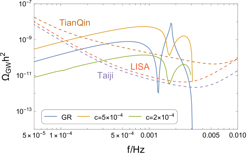
Figure 1: The energy density spectrum of SIGWs generated by the monochromatic primordial power spectrum with the amplitude $\mathcal{A}_{\zeta}=10^{-2}$. The peak scale $k_{p}=10^{12}\text{Mpc}^{-1}$ corresponds to the maximum sensitivity range of TianQin and LISA. The dashed curves represent the sensitive curves of LISA and TianQin, while solid curves represent the energy density spectrum of SIGWs in GR and PV symmetric teleparallel gravity, respectively.

VI Conclusion

The phenomenon of gravitational parity violation has recently attracted significant theoretical interest. In Ref. Li and Zhao (2022), the authors proposed a simple PV gravity model within the framework of symmetric teleparallel gravity, and furthermore studied the linear cosmological perturbations. To evade the strong coupling problem inherent in this model, we introduced a non-minimally coupled boundary term described by action (10). This non-minimally coupled boundary term incorporates connection perturbations $C$ and $D$ into the linear scalar perturbation EOMs (21)-(25), thereby eliminating the strong coupling problem provided the coupling function $g_{1}(\varphi)$ is not constant.

Having resolved the strong coupling problem, we derive the EOMs of linear perturbations and the SIGWs. We then calculated the SIGWs in model (10) during radiation dominated era. To maintain the shift symmetry of the boundary term while ensuring computational tractability, we select the coupling function $g_{1}(\varphi)=c\varphi$. For the parity-violating term, we adopt an exponential coupling form that guarantees time-independent SIGW propagation speeds. Numerically solving the scalar perturbation equations, we calculate the SIGW energy density spectrum with monochromatic power spectrum (81). The non-minimally coupled boundary term not only eliminates the strong coupling problem but also modifies scalar perturbation evolution, producing distinct SIGW signatures, particularly at high frequencies compared to GR. The peaks in the energy density spectrum of SIGWs exhibit an obviously rightward shifting relative to GR predictions, this different feature can be detected by future space-based detectors, such as LISA, TianQin and Taiji.

The linear EOMs in Eqs. (34)-(38) exhibit significant complexity, necessitating numerical solution. Additionally, the metric and connection EOMs are not independent due to the diffeomorphism invariance in action (10). To enable numerical tractability, we therefore impose an constraint $\phi=\psi$, which is the same as that in GR. Consequently, our solutions represent a specific numerical solution subset. The absence of analytic solutions precludes comprehensive analysis of SIGW behavior. Derivation of general and analytic solutions constitutes an important direction for our future work.