SN 2024hpj: a perspective on SN 2009ip-like events

Supernovae (SNe) IIn are terminal explosions of massive stars that are surrounded by a dense circumstellar medium (CSM). Among SNe IIn, a notable subset is the SNe 2009ip-like, which exhibit an initial, fainter peak attributed to stellar variability in the late evolutionary stages, followed by a brighter peak, interpreted as the SN explosion itself. We analyse the spectrophotometric evolution of SN 2024hpj, a SN IIn with signs of precursor activity. Comparing it with similar objects in the literature, we identify star-forming regions as their preferred environments, while a statistical analysis on the observed rate of SNe 2009ip-like indicates progenitor masses around $25-31\;\rm{M_{\odot}}$ and lower. The diversity of spectrophotometric features within the sample suggests that variations in CSM mass and distribution influence the observed characteristics, indicating a shared progenitor scenario.

1 Introduction

Massive stars ($M\gtrsim 8\;\rm{M_{\odot}}$) are thought to end their life in a terminal explosion as core-collapse supernovae (SNe). Throughout their evolution, they can shed their outer layers, which then form a circumstellar medium (CSM) that embeds the progenitor. The mass of the progenitor star, its composition at the moment of explosion, as well as the composition, geometry and distribution of the CSM, give rise to a variety of SNe, which show diversity both in the properties of their light curves and spectra.

The presence of a CSM might be important for the energetics of the SN: when the SN explodes, photons from the ejecta ionise the CSM, producing narrow lines in the spectra and when the ejecta and CSM collide, the shock produces extra energy that powers the light curve. In fact, interacting SNe are usually brighter and have a slower spectro-photometric evolution with respect to non-interacting core-collapse SNe. Moreover, interaction can hide the explosion mechanism, as for example it can mask the ⁵⁶Ni tail with (possibly multiple) shallower decays or rebrightenings, especially if the CSM is structured in shells or clumps (Arcavi et al., 2017). Also the spectra are affected, showing broad boxy lines intertwined with narrow ones (Dessart et al., 2023).

Among all the SN subclasses, SNe IIn (Schlegel, 1990) are brighter, with average peak magnitude $\sim-19\;\rm{mag}$ (Nyholm et al., 2020) and their H-rich spectra show broad ($v\sim 10^{4}\;\rm{km\,s^{-1}}$) emission lines topped by narrower ($v\sim 100\;\rm{km\,s^{-1}}$) components (Smith, 2017) produced in the unshocked CSM, photoionised by shock-collisions occurring in the inner CSM regions (Chugai, 1991; Chugai et al., 2004). On the other hand, if a star is completely stripped of H before the explosion and the CSM is relatively He-rich, the SN will appear as a SN Ibn (Pastorello et al., 2015; Smith, 2017).

Mass-loss is common in massive stars and it can happen via several distinct channels, mainly, steady winds or eruptions. With a steady wind, the mass-loss rate is high and constant for decades (Moriya et al., 2014, $>10^{-3}\;\rm{M_{\odot}\,yr^{-1}}$,), resulting in a large amount of total mass lost before the explosion, while eruptive episodes can account for an enhanced mass-loss rate just before the explosion, possibly, even triggered by pair-instability (Das et al., 2024). Luminous Blue Variables (LBVs), for example, are erupting stars that in some cases have produced SNe IIn (Gal-Yam et al., 2009, e.g.,). Wolf-Rayet (WR) stars, instead, have been associated to SNe Ibn (Pastorello et al., 2007, but see Dwarkadas, 2011). Moreover, it is worth mentioning that stripping of the outer layers can happen also in cases of binary interaction with a companion star. Stars that are stripped with different mechanisms will have a different pre-SN structure and the SN properties will be affected, e.g., binary-stripped SNe have higher ⁵⁶Ni yields that their single-star counterparts (Laplace et al., 2021; Schneider et al., 2021).

Some SNe show a peculiar light curve, with a first peak, called “Event A”, which is less luminous than a SN ($\lesssim-14/-15$ mag at peak) and has a variable duration, from a few weeks (Tartaglia et al., 2016) to months (Elias-Rosa et al., 2016). The spectra of these SNe at this time resemble those of a SN II (Filippenko, 1997), with broad P-Cygni profiles. Afterwards, the light curve brightens once again in the so-called “Event B”, with a higher luminosity at peak and spectra of a SN IIn. The best-studied case was SN 2009ip (Smith et al., 2010; Pastorello et al., 2013; Fraser et al., 2013; Mauerhan et al., 2013; Prieto et al., 2013; Graham et al., 2014; Margutti et al., 2014; Smith et al., 2014, 2022), which showed signs of erratic variability since 2009, then it faded and reappeared again in 2012, with a light curve with the two peaks: Event A and Event B. The mechanism generating the two events of SNe 2009ip-like is disputed. While for many SNe, 2009ip included, Event A was interpreted as the result of pre-explosion outburst activity and Event B as the actual SN explosion (Pastorello et al., 2013; Elias-Rosa et al., 2016; Tartaglia et al., 2016), it is also possible that a faint SN explosion is responsible for Event A, while Event B would be almost entirely due to ejecta-CSM interaction. This latter interpretation was proposed, for example, in the case of SN 1996al (Benetti et al., 2016), based on light curve modeling, although Event A was not observed in that case. More exotic scenarios, such as mergerburst in a binary system, have also been proposed (Brennan et al., 2025), and more recent research seems to support the latter hypothesis that SNe 2009ip-like originate from intermediate mass ($17-20\;\rm{M_{\odot}}$) progenitors, possibly in binary systems (Brennan et al., 2022c; Kilpatrick et al., 2018; Brennan et al., 2025, e.g.,).

In this paper, we present the results of our follow-up campaign of SN 2024hpj, a SN IIn with a light curve composed of a dimmer Event A, a subsequent, brighter Event B and a secondary, dimmer peak after Event B.

The paper is organised as follows: the observations and data reduction procedures are presented in Sect. 2, the spectrophotometric evolution of SN 2024hpj is analysed in Sect. 3, and a comparison with other SNe 2009ip-like and their host environments is given in Sect. 4. Results are discussed in Sect. 5 and conclusions drawn in Sect. 6.

2 Observations and data reduction

SN 2024hpj (a.k.a. PS24dff, GOTO24bjv, ATLAS24gww, ZTF24aaleeji) was first discovered by Rehemtulla et al. (2024) on 30 April 2024 (MJD 60430.9) with magnitude 20.0 mag in the $g$ band of the Zwicky Transient Facility (ZTF, Bellm et al. 2019; Graham et al. 2019; Masci et al. 2019), while the last reported non-detection was also by ZTF, at $m_{g}=19.9\;\rm{mag}$ on 23 April 2024, 7 days before the first detection. It was classified as SN IIn on 11 May 2024 (Pérez-Fournon et al., 2024a). Its coordinates are $\alpha$=17:48:47.759, $\delta$=+37:13:02.01 [J2000] and it is located 2$\aas@@fstack{\prime\prime}$49 N, 2$\aas@@fstack{\prime\prime}$10 E from the centre of the host galaxy WISEA J174847.58+371259.4 (Cutri et al., 2013, a.k.a. GALEXASC J174847.58+371259.4,). The SN position is marked in the finding chart shown in Fig. 1.

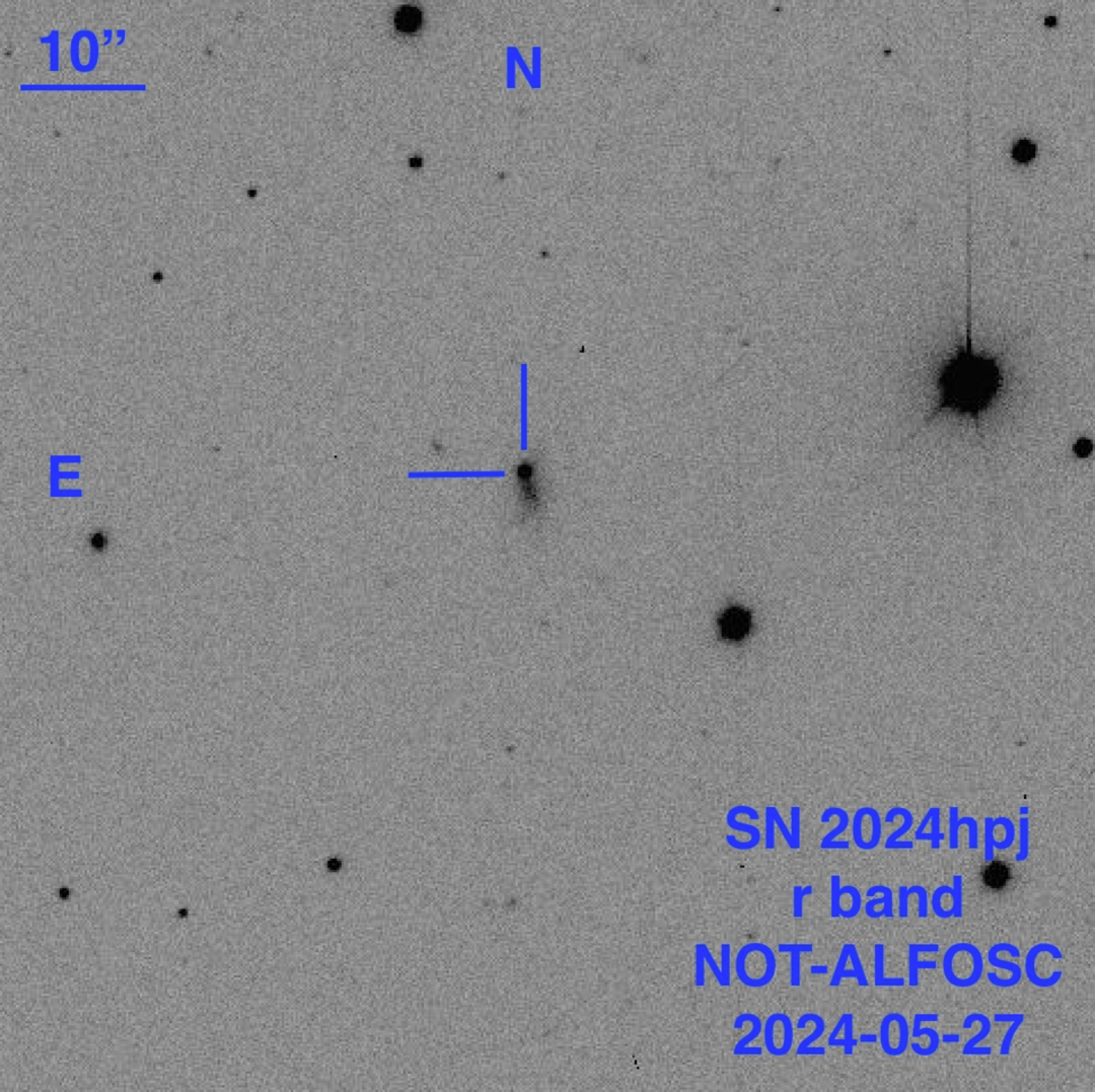
Figure 1: Finding chart for SN 2024hpj. Observed on 27 May 2024 with ALFOSC@NOT in the $r$ band.

2.1 Photometry

We obtained photometry of SN 2024hpj by exploiting our proprietary time at the Schmidt and Copernico telescopes of the Asiago Observatory, INAF (Italy), at the Telescopio Nazionale Galileo (TNG), at the Gran Telescopio CANARIAS (GTC), both located in La Palma (Spain), and at the 2.2m telescope of the Calar Alto Observatory (CAHA-2.2) in Andalucía (Spain). We also made use of the time allocated to the Nordic Optical Telescope (NOT) in La Palma (Spain) through the international collaboration NUTS2 (Nordic-Optical-Telescope Un-biased Transient Survey). Finally, we also retrieved publicly available data from ZTF, the Panoramic Survey Telescope and Rapid Response System (Pan-STARRS, Chambers et al. 2019), and the Asteroid Terrestrial-impact Last Alert System (ATLAS, Tonry et al. 2018; Smith et al. 2020).

Pre-reduction of photometric data was performed using standard techniques in IRAF along with various python packages, notably, astropy (Astropy Collaboration et al., 2022) and affiliated packages (astroquery, ccdproc, photutils). The initial steps included removing the detector signature through bias and flat-field corrections. Following this, a cosmic-ray rejection algorithm was applied to clean the data further.

Astrometric and photometric calibration, as well as SN magnitude measurements, were conducted using routines from the ecsnoopy package. When the SN was too faint (below $\sim 18$ mag), template subtraction was applied to the observed frames to reduce host galaxy contamination. To create the host galaxy templates, archival reference images from Pan-STARRS were utilized. With ecsnoopy, template images were aligned to the pixel grid of science images, and hotpants (Becker, 2015) was then used to convolve the images, ensuring a consistent Point Spread Function (PSF) and photometric scale.

Instrumental magnitudes (or upper limits) were calibrated using photometric zero points derived from local stars, with photometry sourced from Pan-STARRS. For Near Infrared (NIR) observations, the same reduction process was applied, with an additional sky background subtraction step achieved by median-combining dithered images in each filter. In this case, nightly zero points were established using photometry from the Two Micron All-Sky Survey (2MASS, Skrutskie et al. 2003) catalogue. The measured magnitudes are plotted alongside those retrieved from forced photometry on publicly available data by ZTF, ATLAS, and Pan-STARRS in Fig. 2 We were provided with the Pan-STARRS photometry from the Pan-STARRS Search For Transients from the ongoing Pan-STARRS NEO survey (as described in Fulton et al., 2025). There are detections in the $y$ and $w$ band but no historic detections on around 60 nights between MJD=57448 and 60234, through forced photometry.

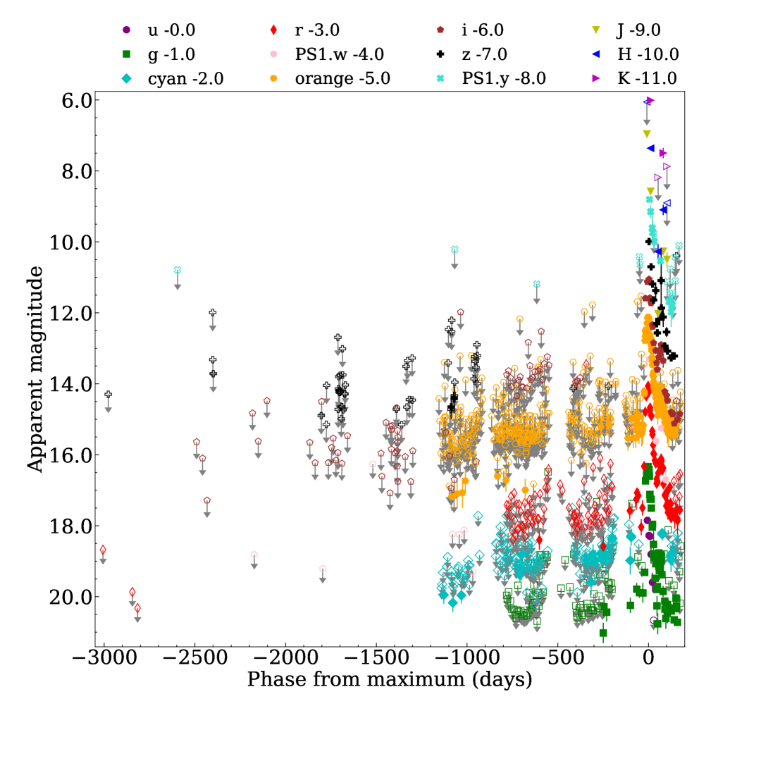
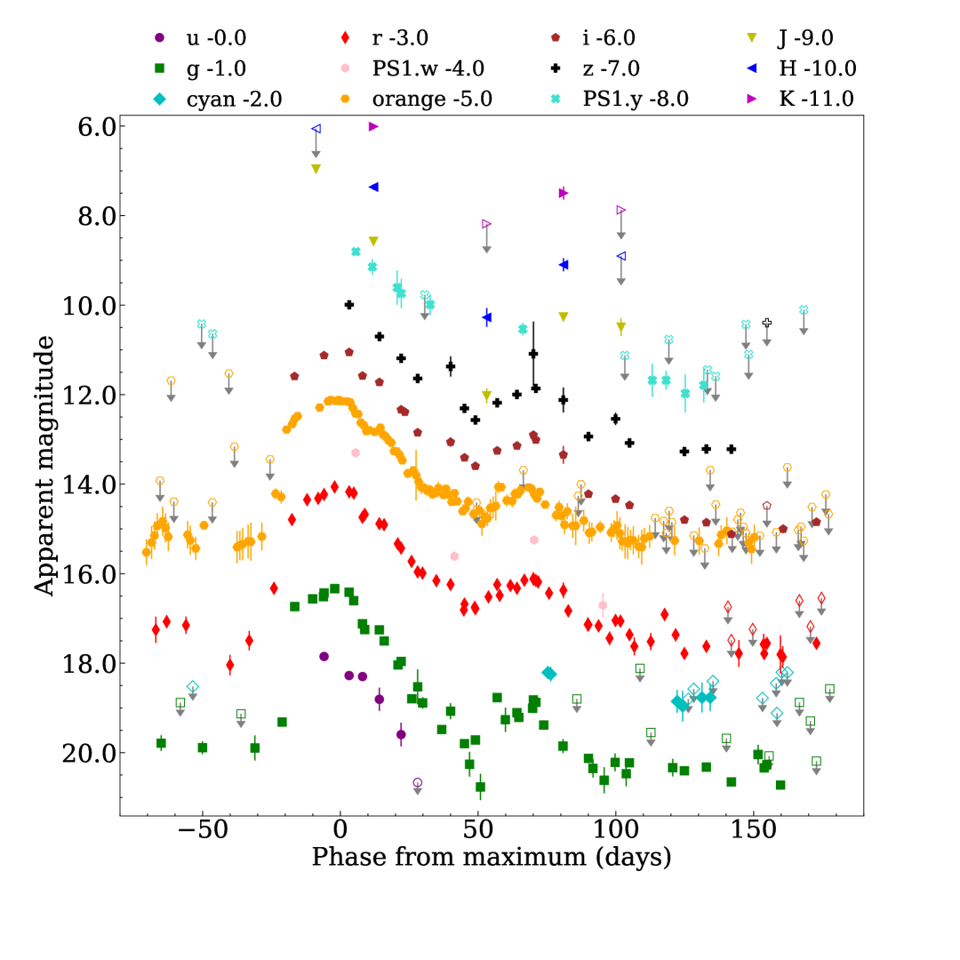
Figure 2: Apparent light curve of SN 2024hpj in the $u,g,r,i,z,J,H,K,cyan,orange,w,y$ bands. A rigid shift is applied for a better visualisation. Top: Complete light curve during the last $\sim 10$ years. Bottom: Zoom in on the Event A+B light curve. Grey arrows and open markers indicate upper limits. Phases are calculated with respect to the epoch of Event B maximum (MJD 60455).

2.2 Spectroscopy

Optical spectra were acquired with the following instruments: the Alhambra Faint Object Spectrograph and Camera (ALFOSC) at NOT, the Device Optimized for the Low Resolution (DOLORES) at TNG, the Calar Alto Faint Object Spectrograph (CAFOS) at CAHA-2.2, and the Optical System for Imaging and low-Intermediate-Resolution Integrated Spectroscopy (OSIRIS+) at GTC.

The same data reduction procedure was applied to all spectra. Using standard IRAF tasks, we corrected the 2D images for bias and flat-field and subtracted the cosmic rays. Then, we extracted the SN trace and calibrated it in wavelength through spectra of standard lamps and in flux with the spectrum of a spectrophotometric standard star. For the spectra taken with ALFOSC and OSIRIS+, the procedure was automated with the pipeline foscgui. Finally, spectra are rescaled in flux to match the photometry at the corresponding epoch. The complete spectral sequence is plotted in Fig. 3.

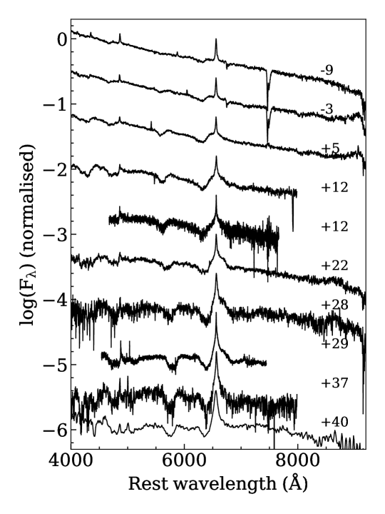
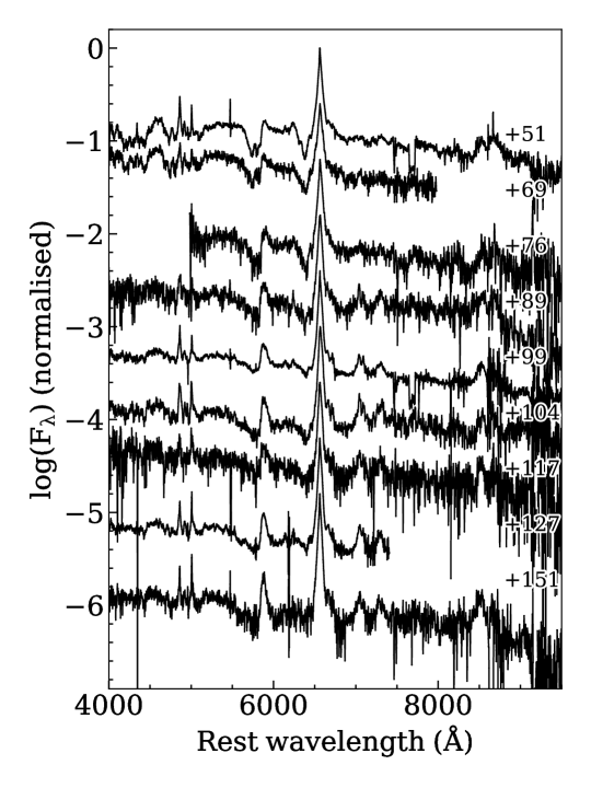
Figure 3: Spectral evolution of SN 2024hpj. All spectra are corrected for redshift and reddening. Numbers close to each spectrum indicate the rest-frame phase since the Event B maximum in the $g$ band.

2.3 Redshift and reddening

We measure the average position of the narrow H$\alpha$ emission present in the SN spectra and derive a redshift $z=0.0187\pm 0.0003$. Adopting the following cosmology $H_{0}=73\;\rm{km\,s^{-1}\,Mpc^{-1}}$, $\Omega_{m}=0.27$, and $\Omega_{vacuum}=0.73$ from Tully et al. (2013), we obtain a distance $d=74\pm 1\;\rm{Mpc}$, which gives a distance modulus $m-M=34.36\pm 0.03$ mag. From the Nasa Extragalactic Database (NED), we find an absorption $A_{V}=0.08\pm 0.01$ mag in the SN direction, therefore, adopting $R_{V}=A_{V}/E(B-V)=3.1$ (Cardelli et al., 1989; Schlegel et al., 1998), we derive $E(B-V)=0.020\pm 0.003$ mag for the Galactic reddening. We do not detect any Na I D lines in the SN spectra associated to the host galaxy. For this reason, hereafter we will assume a negligible contribution of the host galaxy to the total reddening toward SN 2024hpj.

3 Evolution of SN 2024hpj

3.1 Light curve

The multiband light curve of SN 2024hpj is shown in Fig. 2. The shape of the light curve is peculiar: there is a first, low-luminosity peak (the so-called “Event A”) that reaches $g=20.8\pm 0.1$ mag (absolute magnitude $M_{g}=-13.5\pm 0.2$ mag). Constraining the beginning of this phase is challenging due to its faint apparent magnitude, but it appears to last at least 20 days. The first peak is followed by a second, brighter one (“Event B”). The rise to the second peak lasts $28\pm 1$ days, longer than what expected for regular SNe II but in line with interaction-powered SNe. The maximum luminosity reached is $m_{g}=17.4\pm 0.2$ mag ($M_{g}=-16.9\pm 0.2\;\rm{mag}$) on MJD $60455\pm 1$ days. This will be the reference epoch for the peak throughout the paper. The following decline is somewhat slower than the rise, lasting about 50 days, after which the luminosity increases again in all bands, forming an ulterior peak that reaches a maximum luminosity of $g=20.01\pm 0.09$ mag ($M_{g}=-14.3\pm 0.2$ mag) 63 days after the Event B peak. Finally, the light curve begins to decline slightly shallower than the ⁵⁶Co decay timescale until the SN is lost due to solar conjunction.

We also calculated a pseudo-bolometric light curve as follows: magnitudes are converted to flux densities using photometric zero points. The flux within the sampled spectral region is integrated using the trapezoidal rule, assuming zero flux outside the boundaries of the bluer and redder filters and that the colour evolution is constant between two contiguous data points. It is then converted to luminosity based on the distance modulus. The resulting light curve is shown in Fig. 4. By fitting the late-time tail with a linear decline and comparing the slope to that of SN 1987A (Arnett & Fu, 1989), we derive an upper limit for the ⁵⁶Ni mass of $0.07\pm 0.01\;\rm{M_{\odot}}$. We caution that, as mentioned above, the decline is slightly shallower than expected for ⁵⁶Co decay alone and interaction may still contribute significantly to the energy budget.

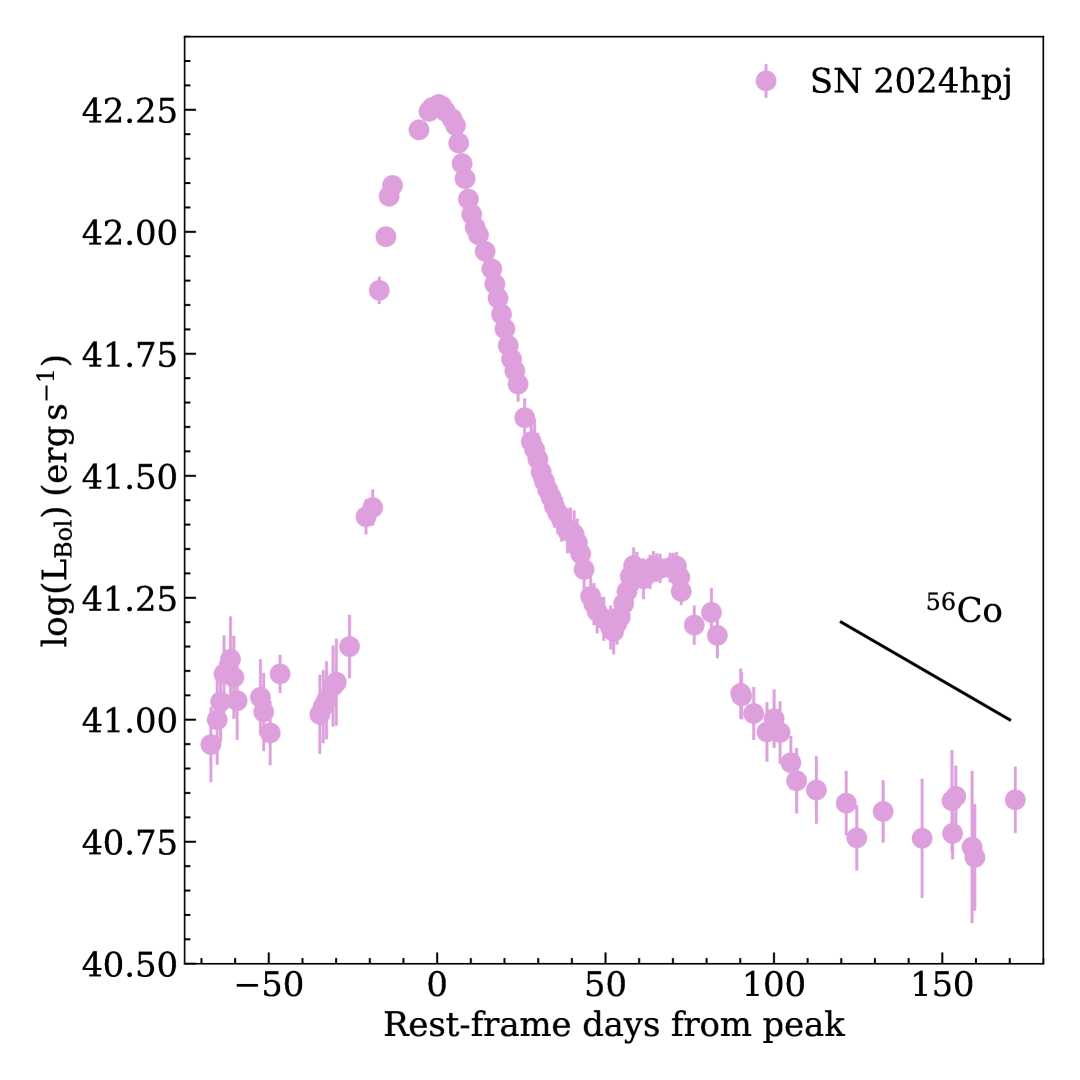
Figure 4: Pseudo-bolometric light curve of SN 2024hpj. For the integration, bands from $u$ to $K$ were used. The expected theoretical decay rate due to ⁵⁶Co is also shown.

Aside from the general declining trend, we noticed that the light curves (both multiwavelength and pseudo-bolometric) show several bumps other than the main ones we already discussed that are probably due to interaction with the CSM. To better investigate this aspect, we applied the same procedure described in Martin et al. (2015). In short, we fit the peak and the decline with two second-order polynomial functions, one between $-20$ and 25 days from the peak and the other between 25–45 and 90–200 days after the peak, thus skipping the secondary bump. The fit was then subtracted and the residuals plotted in Fig. 5. The secondary peak around 50–100 days is the main feature, while the rest of the residuals are scattered around 0. The variation is higher in the early light curve, with undulations peaking around 0 and +25 days in all bands, as well as in the pseudo-bolometric light curve. The bumps also appear slightly higher in amplitude in the redder bands. These residual structures could indicate that the CSM traversed by the ejecta had either changes in density (possibly, even multiple distinct shells) or a non-spherical shape (Kurfürst et al., 2020).

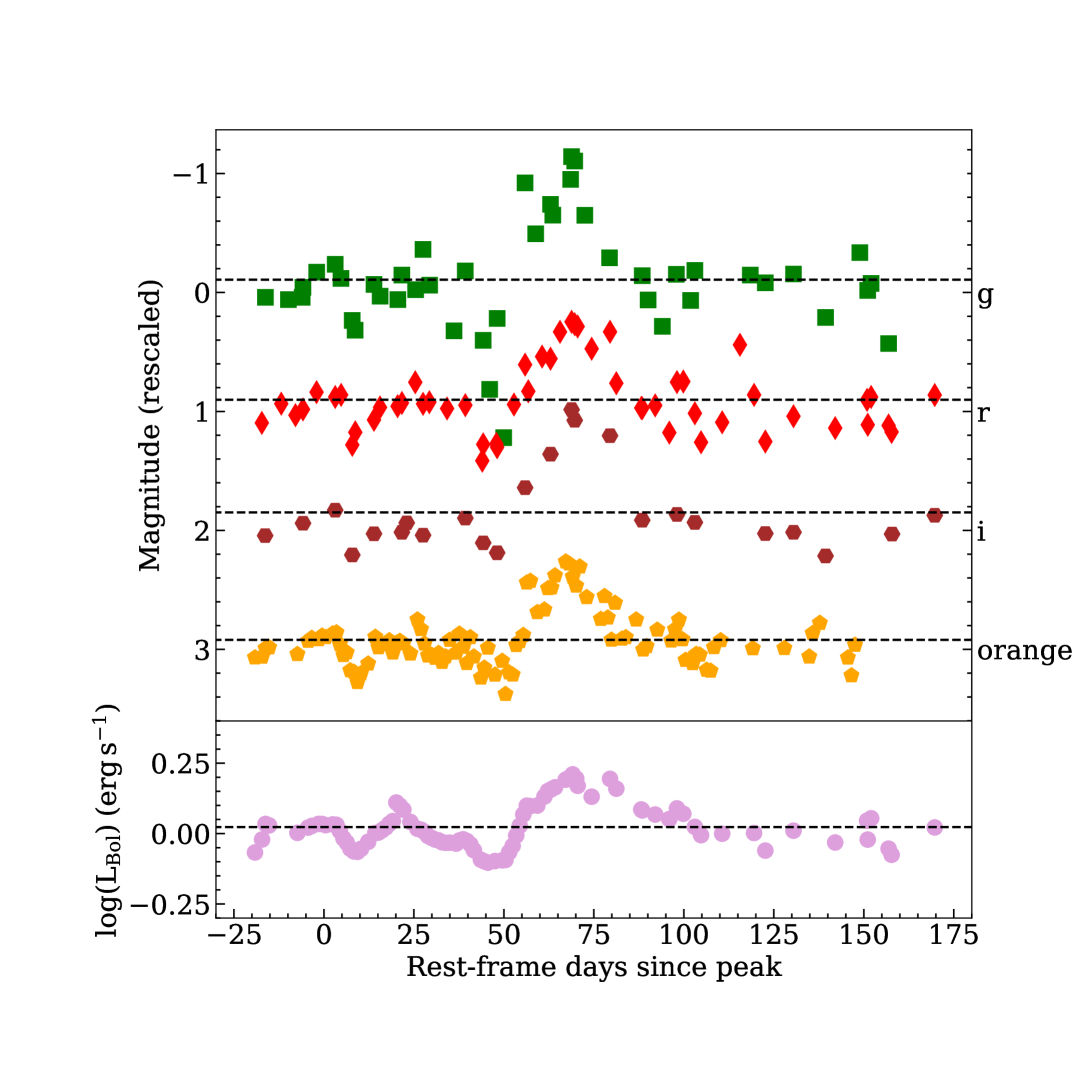
Figure 5: Residuals of the multiwavelength (upper panel) and bolometric (bottom panel) light curves after the peak and decline fit subtraction. Magnitudes are shifted for better visualisation. The dashed lines indicate the mean value of the residuals for each band.

3.2 Spectra

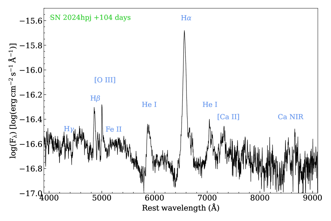
Figure 6: Identification of the most prominent lines on the spectrum of SN 2024hpj taken 104 days after the Event B peak. The spectrum is corrected for redshift and reddening.

The spectral sequence of SN 2024hpj is depicted in Fig. 3, while the line ID is provided in Fig. 6. Unfortunately, we could not obtain any spectra during Event A. The first spectrum, taken 9 days before the Event B maximum, has a blue continuum and shows prominent, broad P-Cygni profiles in both H$\alpha$ and H$\beta$, with a hint of a blue shoulder that could be a proxy of the H shell. The broad lines are superimposed by narrow emission lines (Full- Width-at-Half-Maximum $FWHM\sim 600\;\rm{km\,s^{-1}}$, once corrected for instrumental broadening) that come from the ionised CSM surrounding the SN. The spectrum at $-3$ days is similar to the previous one but with deeper P-Cygni absorptions. He I $\lambda 5876$ is also detected in emission at this phase. Spectra at phases +5 and +12 days show enhanced P-Cygni profiles also from H$\gamma$ and H$\delta$ and a cooler continuum. In addition, at +22 days we detect P-Cygni absorption features indicating several Fe II lines, along to a broad emission corresponding to the Ca II NIR triplet $\lambda\lambda\lambda 8498,8542,8662$. The spectra are similar until +76 days, with only increasing contribution from Fe II multiplets in the bluer part of the spectrum and Ca II NIR in the redder one and [O III] $\lambda\lambda 4959,5007$ either from the host galaxy or the CSM itself. While not detected, we cannot exclude the contamination of other host lines such as H$\alpha$, [N II] $\lambda\lambda 6548,6583$, and [S II] $\lambda\lambda 6716,6731$, which could be blended with the broad H$\alpha$ from the SN. At phase +89 days, we detect blended emission lines from [Ca II] $\lambda\lambda 7293,7326$ and a double-peaked emission that we tentatively identify with He I $\lambda 7065$. Around 100 days after maximum, the P-Cygni absorptions completely disappear and emission lines now have an electron-scattering profile.

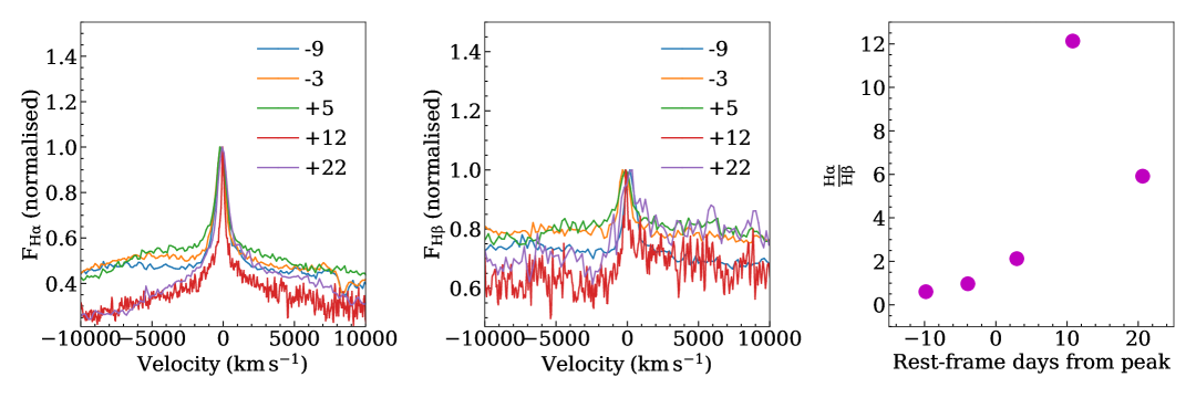
Figure 7: Evolution of H$\alpha$ and H$\beta$ during the first month after the discovery. Left: Evolution of H$\alpha$ in velocity space. Numbers refer to the phase from the peak. Centre: Evolution of H$\beta$ in velocity space. Numbers refer to the phase from the peak. Right: Flux ratios of $\rm{\frac{H\alpha}{H\beta}}$.

In Fig. 7, the evolution in velocity space for H$\alpha$ and H$\beta$ is shown in the first two panels. For both lines the evolution is similar, with a broadening of the feature closer to the peak and a considerable shrinkage shortly after. We also fit the broad emission lines with a Gaussian function to extract an estimation of the flux and plot the flux ratio of $\rm{\frac{H\alpha}{H\beta}}$ in the third panel of Fig. 7. There is an evident evolution from values close to or below the 3.1 limit for case B hydrogen recombination (Osterbrock & Ferland, 2006) to values considerably above it, indicating a probable collisional origin for the excitation.

We fit a black-body (BB) function to the spectral continuum to estimate its temperature and derive the BB radius and luminosity. To ensure a more accurate calculation, we excluded from the fit the areas in the vicinity of major emission lines (H$\alpha$ and H$\beta$). Results are plotted in Fig. 8. The temperature declines rapidly in the first $\sim 60$ days from the Event B peak, from 10000 to 5000 K. The BB luminosity evolution is straightforward, with an initial plateau in the first three spectra followed by a sudden drop. The BB radius, on the other hand, has a more erratic behaviour, but it seems to increase in the first spectra and then decrease, but later than the luminosity and the temperature. A slight increase in the radius could correspond to the hint of plateau that we see before the drop in the light curve; however, there is no evident variation in correspondence of the second bump of the light curve, therefore this is probably a fluctuation due to a poor fit of the spectrum. We do not perform the fit on later spectra since the assumption of BB emission no longer holds at late stages in the evolution (a fit on the pseudo-bolometric light curve confirms this assumption).

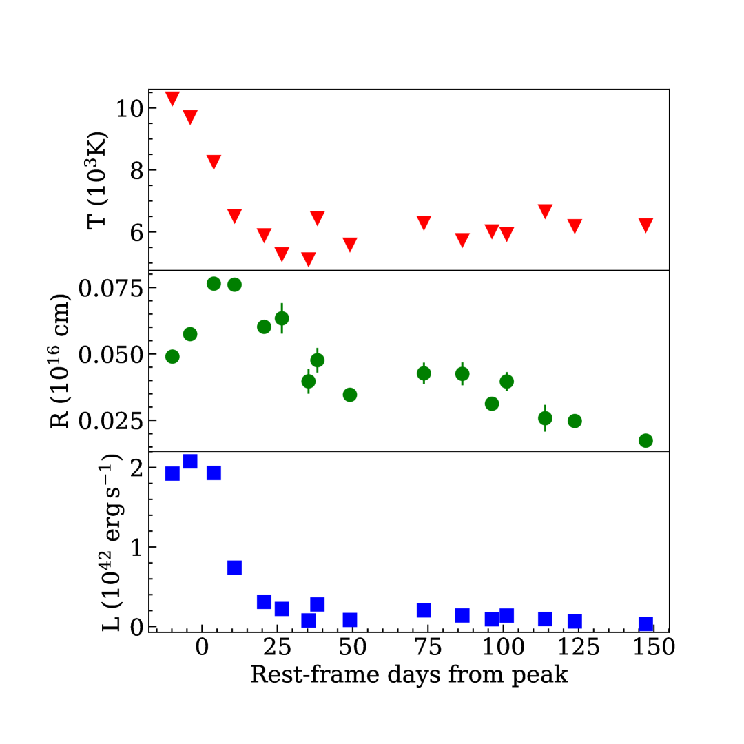
Figure 8: Temperature, radius, and luminosity of the BB fit to the spectra. There is a clear decline in the first $\sim$60 days, while the data sets on a highly variable trend, probably indicating that the assumption of a BB is no longer valid.

To estimate the expansion velocity of the ejecta, we measure the position of the minimum of the P-Cygni absorption on H$\alpha$, He I $\lambda 5876$, and Fe II $\lambda 5169$ and show the results in Fig. 9. The velocity of He I $\lambda 5876$ decreases at all epochs, although we cannot exclude some contamination from Galactic Na I D. The behaviour of Fe II is more erratic, with a slight increase in correspondence of the second peak in the light curve that could however be attributed to scattering. Moreover, it is the line that shows the higher scattering, possibly because of the difficulty of identification in some spectra. H$\alpha$ is the most peculiar line, with an initial, slow decrease in the first three spectra, followed by a rapid drop and then a flattening that finally settles into a plateau at the beginning of the second peak. The different behaviour of the expansion velocity measured on different spectral lines is probably because these lines originate from different regions in the ejecta.

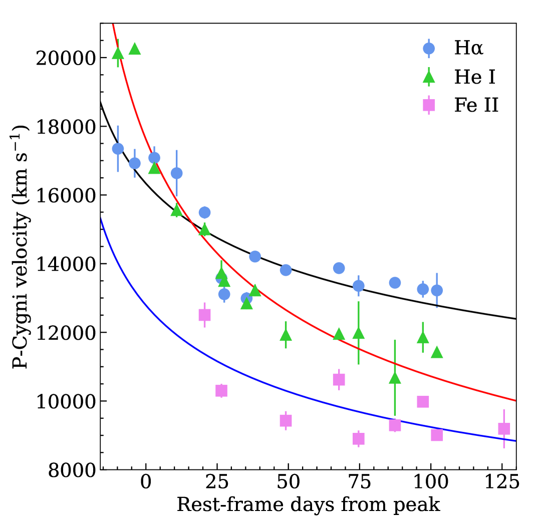
Figure 9: Expansion velocity as measured from the minimum of the broad P-Cygni for H$\alpha$, He I $\lambda 5876$, and Fe II $\lambda 5169$ and power-law fitting (black, red, and blue lines, respectively). We note the similar double trend before and after phase +30 days for H$\alpha$, while He I follows a power-law decline even though, especially at late phases, it is contaminated by Na I D. The Fe II also shows a power-law decline, albeit with some scatter, possibly due to the difficult identification.

We do not detect any narrow ($\rm{FWHM\sim 100\;km\,s^{-1}}$) P-Cygni profiles in the spectra, likely because either the resolution is not enough to properly distinguish this faint feature, or because of the viewing angle, therefore we do not have a clear measure of the wind velocity of the progenitor. However, we take the spectra with the best resolution (at +12 and +29 days from the Event B peak) and measure the FWHM of the narrow H$\alpha$ emission line. This is 4.81 Å and 4.75 Å, respectively (5.47 Å and 5.51 Å not corrected for resolution). The average of the two values translates to an upper limit to the wind velocity of $220\pm 30\;\mathrm{km\,s^{-1}}$, which is significantly higher than the few tens of $\rm{km\,s^{-1}}$ expected for a RSG progenitor but in line with what found for other SNe 2009ip-like (e.g., 2009ip itself had a calculated wind velocity of $550\;\rm{km\,s^{-1}}$, Moriya, 2015). We can take it as an upper limit to the wind velocity that brought the CSM to where it stands at the moment of the explosion. The expansion velocity at the onset of the second bump, which happens about 50 days after the main peak, is $\sim 15000\;\rm{km\,s^{-1}}$ (derived by fitting the expansion velocity from the P-Cygni minima with a power-law decline). We can then estimate the time at which the CSM shell responsible for this bump was ejected, that is, about 1.8 yrs before the explosion.

4 SN 2009ip-like objects

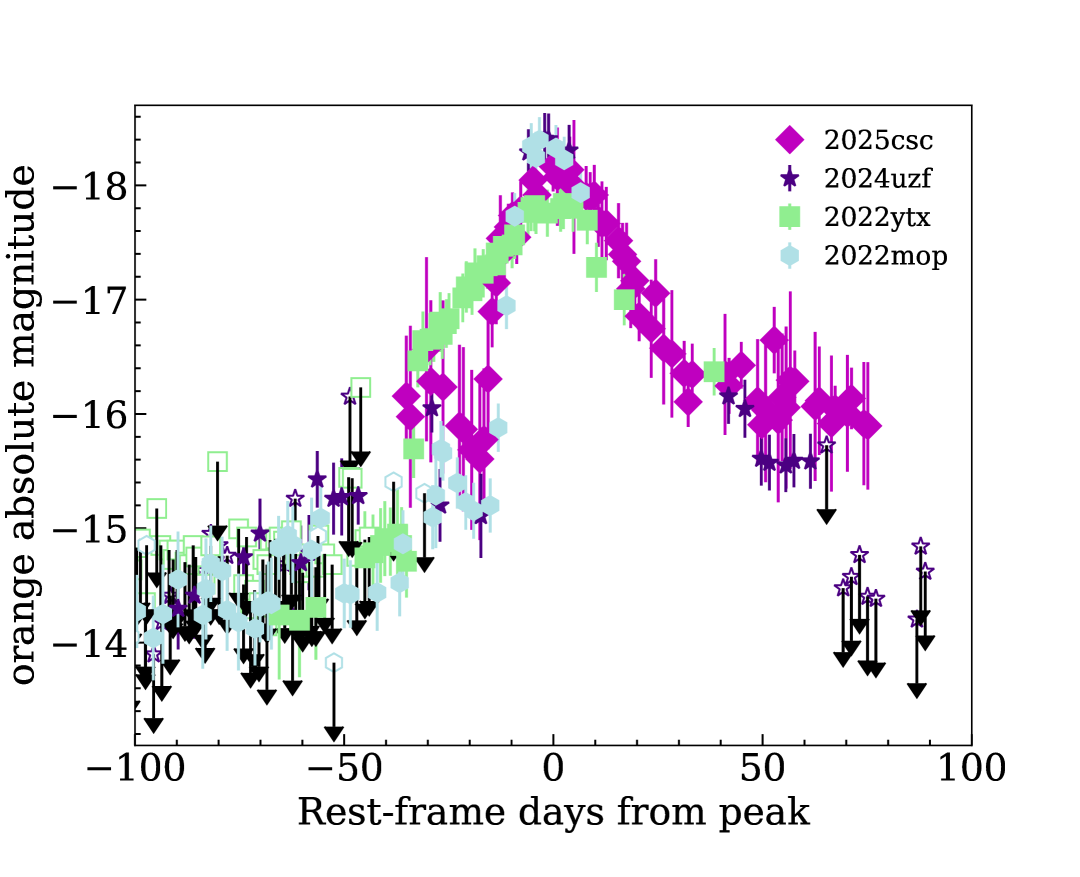
Figure 10: Light curves from the ATLAS forced photometry server in the $orange$ band of the objects we observed as part of the sample presented in this paper. Phases are calculated from the Event B peak. The luminosity of Event B peak and the subsequent decline rate are very similar, while there is some diversity in Event A duration and brightness. Arrows and open markers indicate upper limits.

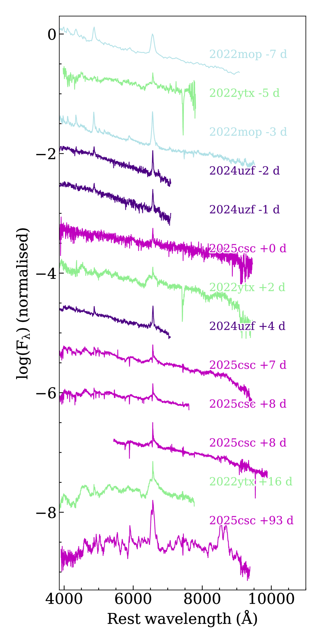
Figure 11: Spectral evolution of the objects we observed as part of the sample presented in this paper. All spectra are redshift- and reddening-corrected and rescaled for better visualisation. Numbers close to the spectra indicate the rest-frame phase from the peak of Event B.

To derive insights on the SN 2009ip-like subclass, we assemble a sample of similar objects. The most important feature in assigning a SN to this class is, of course, the presence of an Event A. However, such an event could easily be missed due to its relative faintness (especially for further away objects) and its duration (especially for those lasting only for a few days). A workaround to this issue is to look at the light curve and spectra. SNe 2009ip-like have spectra during Event B that resemble those of SNe IIn, with prominent narrow emission lines. Their light curves, on the other hand, are more similar to regular SNe IIL (Barbon et al., 1979), with average peak magnitudes ($M\sim-18$) and duration, fading away some 100 days after the peak. Following these criteria, we gathered a sample of 22 comparison SNe, 18 from the literature and four among unpublished objects observed by our group. We shall now briefly introduce these latter and describe their characteristics. The light curve and spectra we gathered for these objects are plotted in Figs. 10–11.

4.1 SN 2022ytx

SN 2022ytx was discovered on 27 October 2022 (MJD 59879.1) by ATLAS with magnitude 18.8 in the $cyan$ band, while the last non-detection was only one day prior (Tonry et al., 2022), at magnitude 19.3 mag in the ATLAS $orange$ band. It was initially classified as SN Ia (Dimitriadis et al., 2022) but was subsequently re-observed and re-classified as a SN IIb with precursor activity on 25 November 2022 (Srivastav et al., 2022). A more careful analysis of the dataset allows us to classify this object as a peculiar Type IIn SN, sharing similarity with SN 1996al (Benetti et al., 2016). The measured redshift is $z=0.026\pm 0.001$, while the Galactic absorption is $A_{V}=0.294\pm 0.004\;\rm{mag}$ from NED.

The $r$ light curve peaks at $-17.862\pm 0.004$ mag and there is a short plateau between $17-36$ days after the Event B peak. In this case, detections of Event A are seen starting around 60 days before the Event B peak in the ATLAS $cyan$ and $orange$ bands and peaking 20 days after at $\sim-15\;\rm{mag}$ in the $orange$ band. The spectra of SN 2022ytx are also similar to SN 2024hpj, with the same composite structure in the H$\alpha$ profile. This SN also shows a narrow P-Cygni profile in the H$\alpha$, with a calculated velocity of $\sim 1000\;\rm{km\,s^{-1}}$.

4.2 SN 2022mop

SN 2022mop was first observed on 11 June 2022 (MJD 59741.6) with magnitude 20.5 in the Pan-STARRS $w$ band (Chambers et al., 2022). Activity from multiple outbursts appeared in the forced Pan-STARRS photometry (Srivastav et al., 2025) and the transient was finally deemed exploded and classified as SN IIn on 4 January 2025 (Sollerman et al., 2025). The measured redshift is $z=0.0170\pm 0.0008$, while the Galactic absorption is $A_{V}=0.150\pm 0.002\;\rm{mag}$ from NED.

Event A peaks at $-15.16\pm 0.02$ mag in the $r$ band 26 days before the peak of Event B, which reaches $-18.40\pm 0.02$ mag. The spectra that are available to us are all taken during the rise to Event B. They are blue and dominated by Balmer emission lines with symmetric, electron-scattering profiles. Recently, Brennan et al. (2025) pointed out the similarities between SNe 2022mop and 2009ip, proposing a merger-burst scenario to explain the two peaks. According to this interpretation, the progenitor of SN 2022mop would belong to a binary system in which the companion star strips the progenitor, which then explodes as a stripped-envelope SN (SESN). The neutron star (NS) remnant of the explosion then sets on an eccentric orbit due to natal kicks and interacts with the inflated companion and the previously-emitted CSM. This interaction would be periodical and thus explain the variability witnessed between the first burst in 2022 and the Event A+B in 2024/2025. Finally, drag forces would decrease the orbital period until an in-spiral sets in and the merge happens, propelling the rebrightening of Event B.

4.3 SN 2024uzf

SN 2024uzf was discovered on 8 September 2024 (MJD 60561.2) by ZTF, with an initial magnitude 20.1 in the $g$ band (Pérez-Fournon et al., 2024b), while the last non-detection was on 5 September 2024 at 20.24 mag in the ZTF $r$ band. It was then classified as SN II on 2 November 2024 (Balcon, 2024). The measured redshift is $z=0.021\pm 0.001$, while the Galactic absorption is $A_{V}=0.07\pm 0.01\;\rm{mag}$ from NED.

The Event A in this SN is quite bright, peaking at $-15.70\pm 0.01$ mag in the $r$ band, and happening 33 days before Event B, which instead peaks at $-18.21\pm 0.01$ mag. The spectra are all taken around the Event B peak. They are reminiscent of typical SNe IIn spectra, with blue continua and Balmer lines in emission with electron-scattering profiles.

4.4 SN 2025csc

SN 2025csc was discovered on 25 February 2025 (MJD 60731.5) by ZTF with magnitude 19.5 mag in the $g$ band (Pérez-Fournon et al., 2025), while the last non-detection was on 23 February 2025 at 20.2 mag in the $r$ band. It was classified as SN IIn on 5 March 2025 (Das et al., 2025). The measured redshift is $z=0.02338\pm 0.00007$, while the Galactic absorption is $A_{V}=0.31\pm 0.04\;\rm{mag}$ from NED.

An Event A in the light curve of SN 2025csc is suggested from ATLAS stacked data, although ZTF only provides detection limits at similar epochs, rising doubts on the significance of the ATLAS detections. If the detections are indeed real, Event A is similar to SN 2024uzf in shape but brighter, peaking at $-16.23\pm 0.04\;\rm{mag}$ in the $orange$ band 31 days before Event B. The latter, instead, is almost identical to SN 2024hpj, reaching $-18.05\pm 0.04$ mag. The spectra are taken all around and after the maximum of Event B. The main feature is an asymmetric H$\alpha$ with a narrow P-Cygni profile that returns a velocity of $\sim 800\;\rm{km\,s^{-1}}$. In the last spectrum at +93 days, Ca II NIR also appears, together with He I $\lambda 5876$ and a forest of Fe II lines.

Interestingly, we note the presence of O I $\lambda 8446$ in emission in all spectra, while O I $\lambda 7774$ is only seen as weak absorption. This could be interpreted as an effect of Bowen fluorescence (Osterbrock & Ferland, 2006, also known as UV pumping,): the Ly$\beta\;\lambda 1025.72$ and the O I $\lambda 1025.76$ lines are in resonance and this pumps electrons from O I to higher levels. The subsequent disexcitation produces O I $\lambda 8446$ but not O I $\lambda 7774$. This mechanism was observed, for example, in intermediate luminosity red transients, which have light curves similar to faint, linearly declining SNe II and progressively redder spectra (Cai et al., 2021, e.g.,). In this context, Valerin et al. (2025) calculated that the Doppler shift necessary to have a perfect match in wavelength is $+12\;\rm{km\,s^{-1}}$, with H and O travelling in opposite directions. Moreover, the Bowen mechanism appears more efficient at later phases, when opacity is lower and Ly$\beta$ photons have less chances to thermalise before encountering O I (Valerin et al., 2025). The Bowen mechanism should also produce O I $\lambda 11287$, therefore detecting this line would confirm our hypothesis. Unfortunately, our spectra lack the wavelength coverage to confirm this, however, this is still a valid interpretation and it could be worth observing the SN at NIR wavelengths for confirmation.

4.5 Comparison with supernovae from literature

As mentioned above, we performed a literature search to select all SNe with a possible Event A + Event B kind of light curve. Moreover, to account for the fact that the Event A may be missed before the SN discovery, we also looked for other SNe IIn that matched the Event B of SN 2024hpj. The SNe we selected are reported in Table 14, together with the main characteristics of their host galaxies.

To compare their light curves, we compute pseudo-bolometric ones by integrating the flux in all available bands as described in Sect. 3.1, using the distance modulus reported in the respective papers (for the unpublished SNe, we applied the same cosmology as for SN 2024hpj, see Sect. 2.3) and taking into account also the additional reddening from the host galaxy when this information was available. For each SN, we used the information from all the available filters. Since the filter coverages varies greatly among the SNe chosen for comparison, with some spanning the whole range from UV to NIR and others with only few filters, we opted to build the pseudo-bolometric light curve of SN 2024hpj each time matching accordingly the available photometry of the comparison SNe. The pseudo-bolometric light curves for all the selected SNe, compared to that of SN 2024hpj, are shown in Fig. 12. In each panel, we also report the wavelength range used to build the pseudo-bolometric light curve.

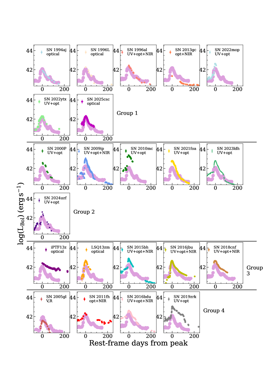
Figure 12: Individual comparison of the pseudo-bolometric light curve of SN 2024hpj (mauve points) with the SNe in the sample. All light curves are matched at the Event B peak (for SN 2022mop, only the period 2024-2025 is shown). Labels indicate the bands used to build the light curve (see text). Four groups are discernible: rise and/or decay time and peak luminosity similar to SN 2024hpj (group 1); more luminous and/or faster declining than SN 2024hpj (group 2); slower declining than SN 2024hpj (group 3); with plateau (group 4).

As can be seen from Fig. 12, four groups are discernible: the SNe that are more similar to SN 2024hpj, both in rise and/or decay time (when covered) and in peak luminosity (group 1); those that are more luminous and/or faster declining than SN 2024hpj (group 2); those that are slower declining and brighter than SN 2024hpj (group 3); those with a plateau (group 4). Notably, SN 2024hpj is the only one with a bright second peak after the Event B one (Nyholm et al., 2017, although iPTF13z showed several smaller bumps, they are not as extreme as for SN 2024hpj and more similar to the undulations of SN 2009ip, rather that a distinct peak,). Finally, all SNe for which late-time data is available have a late-time tail more or less consistent with powering from the decay of ⁵⁶Co. However, as mentioned in Sec 3.1, interaction could still be playing a major role and hiding the ⁵⁶Ni, resulting in shallower slopes and/or higher estimates for the ⁵⁶Ni mass. We also caution that in the case of SN 2009ip, the presence of ⁵⁶Ni was questioned since the decline was faster than expected and interaction was arguably the main powering mechanism (Fraser et al., 2013). This dichotomy probably indicates the same inner engine for all of them and variations in the evolution are most likely due to the mass and distribution of the CSM, which affects the H recombination and the escape time for photons.

For the majority of the SNe in the sample, Event A is visible in almost its entirety. For these, we measure the main peak magnitude and duration of Event A and look for possible correlations with the magnitude of Event B and the separation between the two peaks. The only significant correlation seems the one between the peak magnitudes of Events A and B, which is shown in Fig. 13. A brighter Event A seems to imply also a brighter Event B, in line with what found with respect to SNe IIn with progenitor activity and was interpreted as the presence of a more massive CSM for the brighter events (Ofek et al., 2014; Strotjohann et al., 2021). If interaction is indeed a major contributor during the evolution of SNe 2009ip-like, then an explanation in this sense is likely.

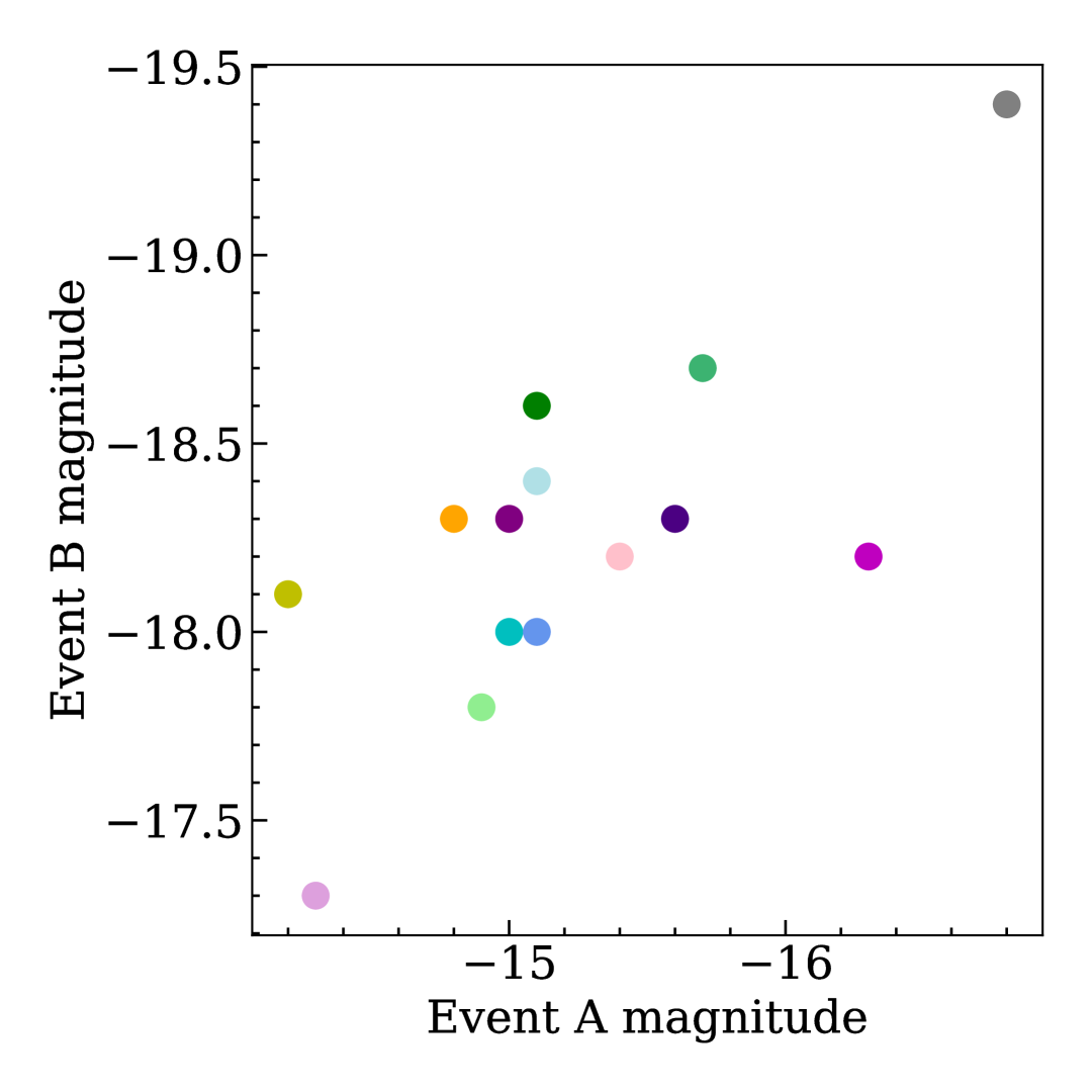
Figure 13: Magnitude at peak of Event B in function of the magnitude at peak of Event A. Measurements were performed on the $r/R$ bands, when available. For the SNe that were not covered during Event A in $r$ (SNe 2025csc and 2022ytx), we elected to perform the measurements in the $orange$ band. Colours are the same as in Fig. 12.

We also compare the spectral features of SN 2024hpj to those of selected SNe among the sample in Fig. 14, where we plot the spectra close to the peak of Event B and about 100 days after it. The spectra around Event B are quite different within the sample: while the quality of the spectrum of SN 2024uzf is too poor to distinguish anything other than a composite H$\alpha$ feature, SNe 2022ytx and 2025csc are the most similar to SN 2024hpj, with the same composite structure in the emission lines, particularly H$\alpha$. SN 2022mop, on the other hand, has a spectrum more similar to SNe 2009ip, LSQ13zm, and 2016bdu (respectively belonging to group 2, 3, and 4 based on the light curve), even if its light curve resembles more those of group 1. These spectra are hotter than the one of SN 2024hpj shown here and with emission profiles dominated by electron scattering that resemble the earlier spectra of SN 2024hpj, albeit without the P-Cygni absorption. While clear differences among spectra of SNe belonging to groups 2, 3 and 4 are not aparent here, we note that SN 2009ip started to show similar composite line profiles to those of SN 2024hpj about a week after its maximum. This indicates that the spectra of these objects evolve quite rapidly around the maximum of Event B, transitioning from higher to lower optical depth when the electron scattering profiles recede and the structure of the line beneath is revealed. The time at which the transition happens is likely due to the amount of material that the shock wave needs to traverse before emerging. Later spectra around 100 days, on the other hand, are more similar, with flat continua that indicate that the emission is no longer a BB, and a shrunk-down H$\alpha$. In the spectra with enough wavelength coverage, the blended triplet of Ca II NIR is always visible.

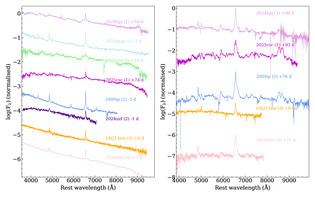
Figure 14: Spectral comparison of SN 2024hpj with selected SNe in the sample. Left: Comparison around the Event B peak. Right: Comparison about 100 days after the Event B peak. Numbers in parenthesis indicate the group based on the light curve (see text). Phases from the Event B maximum are also reported. All spectra are redshift- and reddening-corrected.

4.6 Host galaxies

To infer the general properties of the population of the progenitors, we explored the characteristics of the host galaxies. For each SN in our sample, we retrieved the host morphological classification, preferably via HyperLeda (Makarov et al., 2014) or NED, or the reference papers, when available. In cases where no classification was provided (the host galaxies of SNe 2010mc, 2016bdu, 2018cnf, LSQ13zm, and 2024hpj), we estimated the morphology via direct comparison of the images with those of already classified host galaxies.

Table 1: Characteristics of the host galaxies of the SNe selected for the sample. The morphologic classification is from NED or HyperLeda, when available, or from visual inspection. The position of the SN in the host galaxy is determined upon visual inspection. The apparent radius is from HyperLeda or NED, when available, or from the fitted profile in the cases of SNe 2024hpj and 2010mc. Unconstrained parameters are marked with a $--$.

SN Host Morphology $t$ Position Projected distance $R_{25}$ from centre (kpc) (”) References 2025csc CGCG 142-005 Sb $2.9\pm 1.9$ Spiral arm 2.4 26 $\pm$ 17 This work 2024uzf SDSS J160643.35+484324.6 Scd $6.6\pm 3.0$ Spiral arm 1.9 20 $\pm$ 4 This work 2024hpj WISEA J174847.58+371259.4 S/I (dwarf) $9\pm 2$ Outskirts 1.3 $5.06\pm 0.01$ This work 2023ldh NGC 5875 Sb $3.2\pm 0.6$ Spiral arm 8.6 72 $\pm$ 5 1 2022ytx CGCG 430-046 Sc $5.0\pm 1.5$ Spiral arm 2.7 26 $\pm$ 3 This work 2022mop IC 1496 SB0/a(rs) $0.3\pm 1.3$ Outskirts 16.1 50 $\pm$ 4 This work, 2 2021foa IC 0863 SB0/a?(rs) pec (AGN) $0.4\pm 1.4$ Spiral arm 1.7 34 $\pm$ 7 3,4,5 2019zrk UGC 06625 Scd $6.7\pm 2.3$ Spiral arm 10.1 23 $\pm$ 3 6 2018cnf LEDA 196096 S? $2\pm 2$ Outskirts 2.1 22 $\pm$ 3 7 2016jbu NGC 2442 SBbc $3.7\pm 0.6$ Spiral arm 6.7 140 $\pm$ 10 8,9,10 2016bdu SDSS J131014.04+323115.9 I (dwarf) $10\pm 2$ Outskirts (?) 0.8 4.66 11 2015bh NGC 2770 SBc $5.2\pm 0.6$ Disk/Spiral arm 2.6 104 $\pm$ 7 12,13 2013gc ESO 430-G020 SABc $7.0\pm 0.5$ Outskirts 3.3 70 $\pm$ 10 14 LSQ13zm SDSS J102654.56+195254.8 BCDG $0\pm 2$ Nucleus 0.3 12 $\pm$ 3 15 iPTTF13z SDSS 160200.05+211442.3 I $9\pm 2$ Outskirts 0.7 4.09 16 2011fh NGC 4806 SBc $4.9\pm 0.7$ Spiral arm 4.3 40 $\pm$ 4 17 2010mc GALEXASC J172130.92+480747.6 I $10\pm 2$ Outskirts 0.09 $4.16\pm 0.03$ 18,19 2009ip NGC 7259 Sb $2.9\pm 0.7$ Outskirts 5.3 38 $\pm$ 3 20,21,22,23,24,25,26 2005gl NGC 0266 SBab $1.6\pm 0.7$ Spiral arm 10.3 85 $\pm$ 8 27,11 2000p NGC 4965 SABc $6.7\pm 0.9$ Spiral arm 4.0 74 $\pm$ 3 28 1996al NGC 7689 SABc $5.9\pm 0.3$ Outskirts 5.5 93 $\pm$ 7 29 1996L ESO 266-G010 Sab $2.1\pm 3.0$ Spiral arm 7.9 24 $\pm$ 3 30 1994aj WISEA J090611.68-104005.9 Sc? $5\pm 2$ Spiral arm 5.9 $--$ 31

For the unclassified hosts, we also chose to apply Spectral Energy Distribution (SED) fitting techniques to retrieve some intrinsic properties, mainly, the star formation rate (SFR). We retrieved the NED UV/optical/NIR photometry assuming a 10$\%$ error on each flux (the flux values are included in Table 3). This is done to account for possible systematic errors not included in the catalogue estimates. For the hosts of SNe 2010mc and 2024hpj, we found no available photometry, therefore we modelled pre-explosion Pan-STARRS stacked images in the $g,r,i,z$ bands and retrieved upper limits from the 2MASS point source catalogue. The SED fitting was performed with BAGPIPES (Carnall et al., 2018) using an exponential star-formation history and a Calzetti dust extinction law (Calzetti et al., 1994). The redshift was assumed to be the same as the SNe. The full results of the SED fitting are summarised in Table 2. Our findings highlight that the host galaxies are generally low-mass dwarf galaxies, with the only exception of the host of SN 2018cnf (LEDA 196096), which is a massive galaxy. Two out of five hosts are consistent with being main-sequence galaxies (hosts of SNe 2010mc and 2018cnf), while the remaining three appear to be in a starburst phase (see Appendix A for more details).

Table 2: Results of the SED fitting. The masses are reported in units of solar masses and the $SFR$ in solar masses per year. Upper or lower limits are marked with either the $<95^{\rm th}$ or $>5^{\rm th}$ percentiles, respectively.

HOST	2010mc	2016bdu	2018cnf	2024hpj	LSQ13zm
$A_{\rm V}$ [mag]	$<0.81$	$<0.41$	$0.72^{+0.09}_{-0.08}$	$0.10^{+0.01}_{-0.01}$	$1.45^{+0.13}_{-0.19}$
$\rm Age_{exp}$ [Gyr]	$4.06^{+3.22}_{-2.13}$	$0.47^{+0.21}_{-0.18}$	$7.47^{+1.89}_{-2.48}$	$0.11^{+0.04}_{-0.03}$	$0.70^{+0.57}_{-0.27}$
$\log_{10}(M_{\rm exp})$	$8.41^{+0.20}_{-0.23}$	$5.91^{+0.10}_{-0.12}$	$10.50^{+0.07}_{-0.10}$	$7.58^{+0.12}_{-0.10}$	$8.31^{+0.13}_{-0.14}$
$Z_{\rm exp}/Z_{\odot}$	$--$	$0.76^{+0.50}_{-0.19}$	$--$	$>1.23$	$--$
$\tau_{\rm exp}$ [Gyr]	$8.08^{+3.27}_{-4.08}$	$5.51^{+3.14}_{-2.91}$	$2.77^{+0.98}_{-1.29}$	$6.58^{+4.23}_{-4.40}$	$--$
$\log_{10}(M_{*})$	$8.15^{+0.17}_{-0.19}$	$5.75^{+0.09}_{-0.10}$	$10.19^{+0.06}_{-0.08}$	$7.47^{+0.11}_{-0.09}$	$8.14^{+0.11}_{-0.12}$
$\log_{10}({SFR})$	$-1.36^{+0.18}_{-0.14}$	$-2.79^{+0.13}_{-0.07}$	$-0.09^{+0.08}_{-0.12}$	$-0.48^{+0.03}_{-0.05}$	$-0.56^{+0.10}_{-0.16}$
$\log_{10}(sSFR)$	$-9.50^{+0.34}_{-0.29}$	$-8.54^{+0.21}_{-0.15}$	$-10.28^{+0.13}_{-0.15}$	$-7.92^{+0.02}_{-0.14}$	$-8.70^{+0.21}_{-0.27}$

The position of the transient within the host galaxy is also important to infer clues about the stellar population to which the progenitor belongs. For this step, we visually inspected the images of each SN and determined the position among the following categories: halo, spiral arm, disc, outskirts, and bulge. We then measured the projected distance of the SN from the host galaxy centre. These measurements, together with the host morphological parameter $t$ and the radius that corresponds to a surface brightness of 25 mag ($R_{25}$), are reported in Table 14. From these SNe, we build a volume-limited sample by establishing a cut at 100 Mpc (z=0.024). Moreover, we consider that SNe discovered before SN 2009ip were not classified as 2009ip-like, hence we might have missed some contributors. Therefore, SNe discovered before 2009 are taken out of the filtered sample. With these criteria, we plot the distribution of the host morphology and the distance of the SNe from the centre of the host galaxy in Fig. 15. While small, dwarf galaxies for which it was difficult to determine the morphology class appear dominant in the volume- and time-limited sample, there is a strong contribution also from spiral and irregular galaxies. Regarding the position of the explosion site, SNe seem to explode preferably within a few kpcs from the host centre. We caution that this measurement is a lower limit, as the de-projected distance could be higher. Moreover, as can be seen from Table 14 and the second panel of Fig. 15, the position is generally marginal, either in a spiral arm or downright in the outskirts, and the majority of SNe are found well outside the bulge. Thus, the stellar populations surrounding the explosion sites are likely young and blue.

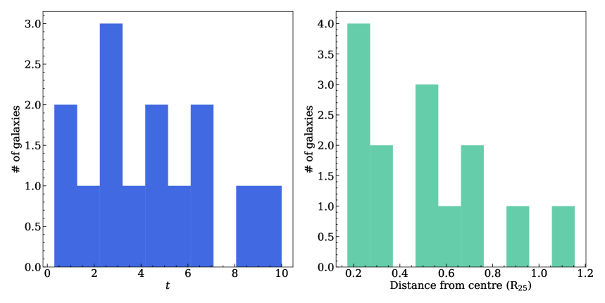
Figure 15: Distribution of host morphology according to the $t$ parameter and distance of the SN from the centre of the host galaxy for the SNe in the sample limited in volume (within 100 Mpc) and time (discovered after 2009).

Classical SNe II with these absolute magnitudes and evolution timescales are associated with $\sim 15-20\;\rm{M_{\odot}}$ Red Supergiants (Boian & Groh, 2020, RSGs,) stars (Smartt, 2009; Morozova et al., 2017, e.g.,). However, the environments in which the SNe 2009ip-like in our sample preferentially explode seem to point toward more massive progenitors. While older (before $\sim 2013$) SNe are mostly found in grand design spiral galaxies, the trend with newer SNe in the sample seems to indicate more dwarf galaxies, which also reflects our findings on the SED fitting. This could be a selection effect: in the past, SNe were discovered by chance while observing nearby, massive galaxies. Nowadays, instead, surveys are focusing more on the distant Universe and thus observing more smaller galaxies that were previously overlooked because they were too faint to be reached with older instruments. However, it is interesting to note that Tartaglia et al. (2016) classified the host of LSQ13zm as a Blue Compact Dwarf Galaxy (BCDG, Haro, 1956; Zwicky et al., 1961). As the name suggests, these are blue, small galaxies with low luminosity and metallicity, and some of them have spectra that are reminiscent of H II regions and high SFRs (Fanelli et al., 1988; Cairós et al., 2001). They could therefore be favourable hosts for this kind of SNe.

5 Discussion

The progenitors of SNe 2009ip-like are still debated. While Event A is consistent with being a stellar eruption, the luminosity of Event B resembles more that of a terminal explosion. However, in SN 2011fh, there still appears a source at the SN position only slightly fainter than three years before the major brightening in 2011, and thus the star may not have exploded (Pessi et al., 2022; Reguitti et al., 2024).

Many authors claimed LBVs as possible progenitors of SNe 2009ip-like (Kashi et al., 2013; Soker & Kashi, 2013; Smith et al., 2014, e.g.,), as an LBV could easily produce the observed CSM during the eruptive phases, which tend to happen close to the explosion. Therefore, the CSM would not have the time to get far from the progenitor and interaction could onset soon after the explosion. Several mechanisms are thought to provoke the eruptive mass-loss phases in LBVs, among which there are stripping from a binary companion (Kashi & Soker, 2010) or pair instability processes (Smith & Owocki, 2006; Woosley et al., 2007, PI,). The progenitor of SN 2005gl was most likely a LBV (Gal-Yam et al., 2007) and its spectra are similar to those of SNe 2009ip-like (Pastorello et al., 2018). Moreover, other SNe 2009ip-like have high calculated progenitor masses (e.g., SN 2011fh has a reported progenitor mass of $35-80\;\rm{M_{\odot}}$, in line with an LBV scenario, Pessi et al., 2022, although we recall that the progenitor is likely yet to explode, Reguitti et al. 2024). However, these estimates assume that the progenitor was in a quiescent state, which is unlikely to be the case, especially when considering such highly variable stars as LBVs. If the progenitor was observed during even a minor outburst, the mass would be dramatically overestimated. Therefore, the identification of the progenitor in pre-explosion images poses only an upper limit to its mass. Moreover, LBVs may not be the only type of stars to produce a high mass-loss before the explosion, as authors have claimed WR stars (Dwarkadas, 2011) or even RSGs as viable alternatives.

A PI-induced explosion could produce a late-time tail with the decay rate expected from a ⁵⁶Ni-powered light curve (Kasen et al., 2011). However, the peak luminosity of the SNe in our sample is relatively faint, far from what PI models predict (Nagele et al., 2024, $\sim 10^{44}\;\rm{erg\,s^{-1}}$,). Pulsational PI (PPI) could easily explain the dense CSM ejected shortly before the explosion, as well as the shallower late-time decay discussed in Sect. 3.1. However, this scenario is not supported by the measured expansion velocity: models of PPI suggest low velocities (Woosley, 2017, $\lesssim 5000\;\rm{km\,s^{-1}}$,), while our measurements on several emission lines indicate velocities at least twice faster, as can be seen from Fig. 9 (although models of Eta Carinae expansion velocities indicate that some layers might be expanding faster, at a rate $>10000\;\rm{km\,s^{-1}}$, due to asymmetric eruptions, the average velocity of the main eruption is still $<600\;\rm{km\,s^{-1}}$, Smith et al., 2018). Also Smith et al. (2022) discussed the PPI scenario for SN 2009ip, finding that it could not explain the series of weak ejections before the major burst, as well as the H retention observed in SN 2009ip, contrary to PPI models that predict complete ejection after the first pulse. Moreover, we observe that, in most cases, the late-time decline rate of the light curve is consistent with radioactive ⁵⁶Co, whereas PPI can vary and depends on the amount of mass ejected. While there is a chance that a PPI SN could mimic the late-time evolution of ⁵⁶Co, it is unlikely to happen for all the SNe in the sample.

Another progenitor scenario for SNe 2009ip-like was proposed more recently in the case of SN 2016jbu, in response to observations from the Hubble Space Telescope (HST) that showed a possible Yellow Supergiant (YSG) $17-30\;\rm{M_{\odot}}$ star (Van Dyk, 2017; Reguitti et al., 2025, like the progenitors of SNe IIb,), whose uncertainty depends on the reddening at the explosion site and the flux overestimation in the HST filters (Kilpatrick et al., 2018; Brennan et al., 2022c). The mass-loss in this case would be due to waves that generate in the core during the latest stages of nuclear burning (Quataert & Shiode, 2012, O/Ne onward, depending on the mass,). Another possibility for R/YSG stars to lose enough mass to create the dense CSM observed is if they belong to binary systems. The merge of the two binary components would then be responsible for the SN main peak, while the precursor event is due to the energy released during the last inspiral (Schrøder et al., 2020). Another, similar interpretation was also proposed for SN 2022mop (Brennan et al., 2025), in which a SESN created a NS that interacted with the companion. In this case, Event A would be determined by the interaction between shells ejected by the companion star, while Event B could either be due to the jet produced in the merging between the NS and the secondary interaction with the CSM, or to the explosion of the companion.

There are no definite indications in favour of one or the other scenario, on the contrary, it is possible that all mechanisms contribute to the population of SNe 2009ip-like. Taddia et al. (2015) found that SNe IIn with a small amount of CSM come from RSGs, while those with longer duration and stronger interaction (and thus higher luminosity) are consistent with LBV progenitors. If this dichotomy applies to 2009ip-like objects as well, more luminous and longer-lasting transients may come from higher-mass stars, possibly losing mass through PI processes. On the other hand, those with light curves more similar to regular SNe II may be more easily explained by a YSG progenitor in a binary system, perhaps even as the result of a merging event. While we observe some diversity in peak luminosity and duration (although a longer duration could simply be due to SNe being closer and thus observable for longer), none of the SNe in the sample reaches the values of the LBV products suggested by Taddia et al. (2015) (Taddia et al., 2013, $M_{r}<-19$ mag, decline rate $\lesssim 0.7\;\rm{mag\,(100\penalty 10000\ days)^{-1}}$,). Hence, the LBV contribution to this sample, at least, is probably limited. Considering also SNe IIb (whose progenitors are YSGs), as well as the cases of transitional SNe such as SN 2021foa itself, it appears that there is a continuum of properties among these transients (Reguitti et al., 2022; Farias et al., 2024; Gangopadhyay et al., 2024). The amount of H envelope lost in eruptive episodes before the explosion determines whether the SN will be a IIL, 2009ip-like, IIb, transitional Ibn, or completely stripped Ibn. The H could even form a plateau after the Event B peak, as can be seen in SNe 2019zrk and 2023ldh, if part of the envelope is still retained by the progenitor and recombines after the ejection. The amount of H retained could vary based on many variables, including the progenitor mass (with lower masses retaining more envelope) and the metallicity (with metal-rich progenitors shedding more layers). In the case of SN 2024hpj, however, the significant rebrightening after Event B is more easily explained with a collision between the ejecta and a thin shell of CSM. The mass-loss in YSG could be triggered by waves in the core, as mentioned before, and the presence of a companion may enhance it (Yoon et al., 2017, as is the case for SNe Ib and IIb,). Finally, the environment may also play a role: SNe 2009ip-like in our sample do not seem to favour extremely marginal regions (especially for those in dwarf galaxies) of their host galaxies, which, however, are mostly dwarf, star-forming ones. We can therefore assume that the metallicity in those regions is low, as was already noted for SN 2009ip itself (Smith et al., 2016), and the mass-loss rate is inhibited in such environments with respect to the more metal-rich ones. This could also explain why they retain part of their H envelope and are not entirely stripped (although we note that Moriya et al. (2023) found that, while SNe IIn belong to metal-poor regions and younger stellar populations, the CSM density does not correlate with the metallicity, indicating that it does not influence the stripping mechanism). In Galbany et al. (2018), CCSNe are generally found in regions with high SFR but for SNe IIb, which instead prefer a lower and narrower SFR distribution. The age of the stellar populations is young for all CCSN subtypes but again SNe IIb are slightly older than SNe IIn, albeit there is no significant difference in the metallicity, which is low for all subtypes. This is in line with a binary progenitor scenario, which can allow older, lower-mass stars to be stripped and form a CSM around the pair.

A possible approach to disentangle the progenitor scenarios is to compare the rate of SNe 2009ip-like in our sample to the theoretical ones. A search in TNS indicates 1480 classified core-collapse SNe in the last 15 years within 100 Mpc, of which 69 are SNe IIn, that is $\sim 5\%$, in line with Graur et al. (2017). In our sample of SNe 2009ip-like, we find 14 SNe within 100 Mpc since 2009. Assuming our sample is complete, this represents a fraction of $\sim 20\%$ of SNe IIn, or $\sim 1\%$ of all CCSNe. However, considering an absolute magnitude around $-14$ mag for a typical Event A, an outburst at 100 Mpc would have a peak apparent magnitude $>21$ mag, which is outside the limits of ZTF or ATLAS, and while Pan-STARRS could in principle detect that, the cadence is usually too relaxed to catch the evolution. If we limit ourselves to a volume of 50 Mpc, instead, the peak apparent magnitude would be $\sim 19.5$ mag. Within 50 Mpc, TNS reports 327 classified CCSNe (of which 14 are SNe IIn) since 2009. In out sample of SNe 2009ip-like, instead, there are 7 SNe discovered since 2009, making them the $\sim 2\%$ of CCSNe. These estimates, however, have several limits. Some SNe are too faint to be detected, others are obscured by dust, and others still are not spectroscopically classified, and it is estimated that a fraction of $\sim 40\%$ is lost (Abac et al., 2025) due to these reasons. Moreover, many SNe that are initially classified as type IIn can be contaminated by host galaxy lines, or show flash ionisation features that disappear soon after the explosion. For example, Ransome et al. (2021) systematically re-classified SNe IIn in TNS, finding that many were consistent with H II contamination, gap transients, flash ionisation, or showed no narrow lines at all. This implies that the $1-2\%$ fraction is only a lower limit and SNe 2009ip-like could be more abundant. Even taking these caveats into consideration, the small fraction of SNe 2009ip-like indicates that they are rare. Therefore, the first possible explanation is that they come from massive progenitors. Assuming a Salpeter initial mass function (IMF, Salpeter, 1955) between $0.1-100\;\rm{M_{\odot}}$ within a volume of 100 Mpc, Abac et al. (2025) find a star formation rate (SFR) of $\sim 0.018\;\rm{M_{\odot}\,yr^{-1}\,Mpc^{-3}}$ based on observations of IR and UV luminosity functions by Bothwell et al. (2011). To determine the plausible mass of the progenitors of SNe 2009ip-like, first we calculate the CCSN rate as was done in Abac et al. (2025) with the IMF and SFR discussed above within a range of progenitor masses $8-40\rm\;{M_{\odot}}$ and vary the integration limits to find the interval that reproduces the $2\%$ observed fraction of SNe 2009ip-like within 50 Mpcs over 15 years, obtaining the range $31-34\rm\;{M_{\odot}}$. If the progenitors of SNe 2009ip-like belong indeed to binary systems, however, there is the additional consideration that only about $70\%$ of massive stars are in binaries that will interact (Sana et al., 2012; Eldridge et al., 2017). Moreover, if the interpretation of a merger event (Brennan et al., 2025) is correct, only one SN 2009ip-like event will happen per pair of suitable progenitors. With these considerations, we find the best results with the range $25-31\rm\;{M_{\odot}}$ when considering a 10% maximum difference between the observed and calculated rates, in line with previous studies (Bilinski et al., 2015; Kilpatrick et al., 2018; Brennan et al., 2022c). We also caution that the procedure assumes that all progenitors with the correct mass will give rise to SNe 2009ip-like, whereas it is probable that, depending on the mass-loss during the evolution and especially binary interaction, only a fraction of the progenitors will produce SNe 2009ip-like, while others will give rise to SNe IIb, IIL, and Ibn.
Another explanation for the rarity of SN 2009ip-like events is that the system configuration is very peculiar. If indeed they come from a merger-type scenario, factors such as delay time, orbital separation, pre-explosion mass-loss, and common envelope phase come into play, painting an extremely complex picture.
Finally, sample selection plays a role. To build our sample, we selected SNe that had detected Event A+B and added to these a handful of SNe with a light curve matching the Event B of SN 2024hpj. However, it is likely that some were missed. All these considerations imply that the ranges we find are upper limits: if SNe 2009ip-like were a higher fraction of CCSNe, then the progenitor mass range would be larger and more extended towards lower masses. Future works will expand on this, considering also Event A-less SNe to build a more complete sample.

6 Conclusions

We have shown the results of the spectrophotometric analysis of SN 2024hpj. The SN showed a peculiar light curve, with a pre-explosion Event A, a major peak (Event B) and a secondary peak probably due to interaction with the CSM. The spectra are also compatible with interaction, showing as narrow emission lines on top of a fast-expanding photosphere.

We built a sample of SNe 2009ip-like and analysed their properties. The light curves are divided in four groups based on their resemblance with SN 2024hpj. Those in group 1 (the most populated one) have similar rise and decay times, as well as a comparable peak magnitude. Group 2 is the second-most populated one and features SNe similar to SN 2009ip, with brighter peaks and faster declines with respect to SN 2024hpj. The SNe in group 3, on the other hand, are more slowly declining, while those in group 4 show a plateau after the peak of Event B. The spectra of SNe belonging to group 1 are also similar (except for SN 2022mop), showing a composite H$\alpha$ emission around the Event B peak, while SNe belonging to the other groups are all similar, blue and with symmetric line profiles. For the SNe that showed a clear Event A, we also found a positive correlation between the peak magnitude of Events A and B, possibly, indicative of a more massive CSM for the brightest events.

Regarding the host galaxies, older SNe are preferably found in the spiral arms of grand-design spiral galaxies, while more recently-discovered ones seem to prefer dwarf ones. While this could be due to a selection effect, they are in both cases associated with regions of high SF. Finally, we found that, from a statistical point of view, SNe 2009ip-like originate from a range of intermediate to high progenitor masses ($25-31\rm{\;M_{\odot}}$). However, this estimate is only an upper limit, since it is sensitive to the fraction of SNe that are lost due to obscuration, faintness, or that are not classified, as well as the specific configuration of the system. Moreover, this specific SN class is difficult to narrow down due to the fact that the Event A could be easily missed. The synergy of upcoming surveys and instruments aimed at monitoring and classifying the transient sky, such as the Vera Rubin Legacy Survey of Space and Time (LSST, Ivezić et al., 2019) and Son-Of-X-Shooter (SOXS, Schipani et al., 2018), will offer the possibility to probe the evolution of these transients with more systematic, complete follow-up campaigns, thus shedding light on this matter.

Appendix A SED fitting

In Table 3, we report the available photometry for the host galaxies of SNe 2010mc, 2016bdu, 2018cnf, LSQ13zm, and 2024hpj as reported by NED, assuming a 10$\%$ error on each flux. This is done to account for possible systematic errors not included in the catalogue estimates. For SNe 2010mc and 2024hpj no photometry was available, so we used $g,r,i,z$ and $J,H,K$ stacked images retrieved from Pan-STARRS and 2MASS, respectively. We checked the morphology in the Pan-STARRS images, finding two spatially resolved galaxies near the location of the SN. For the 2MASS data, we checked the point-source catalogue, finding no obvious detection for either galaxy. Hence, we adopted the magnitude upper limits corresponding to the 10$\sigma$ point source detection depths.

Table 3: Flux densities in $\mu$Jy of the host galaxies of the SNe. Upper limits for the 2MASS photometry are given as $10\sigma$ depths for point sources.

Band	2010mc	2016bdu	2018cnf	LSQ13zm	2024hpj
UV
GALEX/FUV	$--$	$--$	$--$	10.43	140.96
GALEX/NUV	$--$	$--$	$--$	9.12	150.59
Optical
SDSS/u	$--$	2.90	$--$	27.97	$--$
Johnson/B	$--$	$--$	1371.00	$--$	$--$
SDSS/g	$--$	5.20	$--$	68.00	$--$
Pan-STARRS/g	40.87	$--$	$--$	$--$	9.02
SDSS/r	$--$	6.39	$--$	107.27	$--$
Pan-STARRS/r	54.43	$--$	$--$	$--$	11.48
SDSS/i	$--$	5.46	$--$	112.31	$--$
Pan-STARRS/i	58.62	$--$	$--$	$--$	12.69
SDSS/z	$--$	3.30	$--$	121.46	$--$
Pan-STARRS/z	71.04	$--$	$--$	$--$	17.65
NIR/IR
2MASS/J	$<487.63$	$--$	14343.32	$--$	$<406.34$
2MASS/H	$<692.31$	$--$	11141.36	$--$	$<574.25$
2MASS/K	$<1047.93$	$--$	9712.57	$--$	$<722.99$
WISE/W1	$--$	$--$	7287.31	306.57	158.42
WISE/W2	$--$	$--$	4089.22	$--$	89.53
WISE/W3	$--$	$--$	9867.09	$--$	340.68
WISE/W4	$--$	$--$	15379.57	$--$	$--$

Given both the hosts of SNe 2010mc and 2024hpj are resolved, we applied surface brightness modelling techniques using PyAutoGalaxy (Nightingale et al. 2021) to model their light distribution and retrieve their photometric properties. The host of SN 2024hpj seems to be dominated by a disc structure with visible star-forming regions/spiral structure, especially dominating in the bluer bands, therefore, we fitted an exponential profile for the disc and a pixelisation (see Nightingale et al. 2018) for the spiral structure. The host of SN 2010mc, instead, shows a more diffuse featureless light distribution that we fitted using a Sérsic profile alone as model for the surface brightness. For both galaxies, we fitted each Pan-STARRS band together using shared parameters for the flattenings, Sérsic indices and position angles while leaving free the effective surface brightness and effective radius to allow the model to slightly adapt to each specific band. In the case of the host of SN 2024hpj, the pixelisation shape and regularisation constant were shared across all bands. We also computed the isophotal diameter at which the surface brightness is 25 mag ($D_{25}$) by extracting the last 1000 model images from the fits chains in the PANSTARRS $r$ band, converted them to surface brightness, and lastly computed the area in pixels having lower surface brightness than 25 mag arcsec^-2. These areas were circularised to derive the $D_{25}/2$ through $D_{25}/2[{\rm pixel}]=\sqrt{A[{\rm pixel}]/\pi}$. The $D_{25}$ was then converted to arcsec by multiplying by the pixel scale. We obtained $D_{25}=10.12\pm 0.02$ arcsec and $D_{25}=8.32^{+0.06}_{-0.05}$ arcsec for 2024hpj and 2010mc respectively. The results of the fit are shown in the summary plots in Fig. 16.

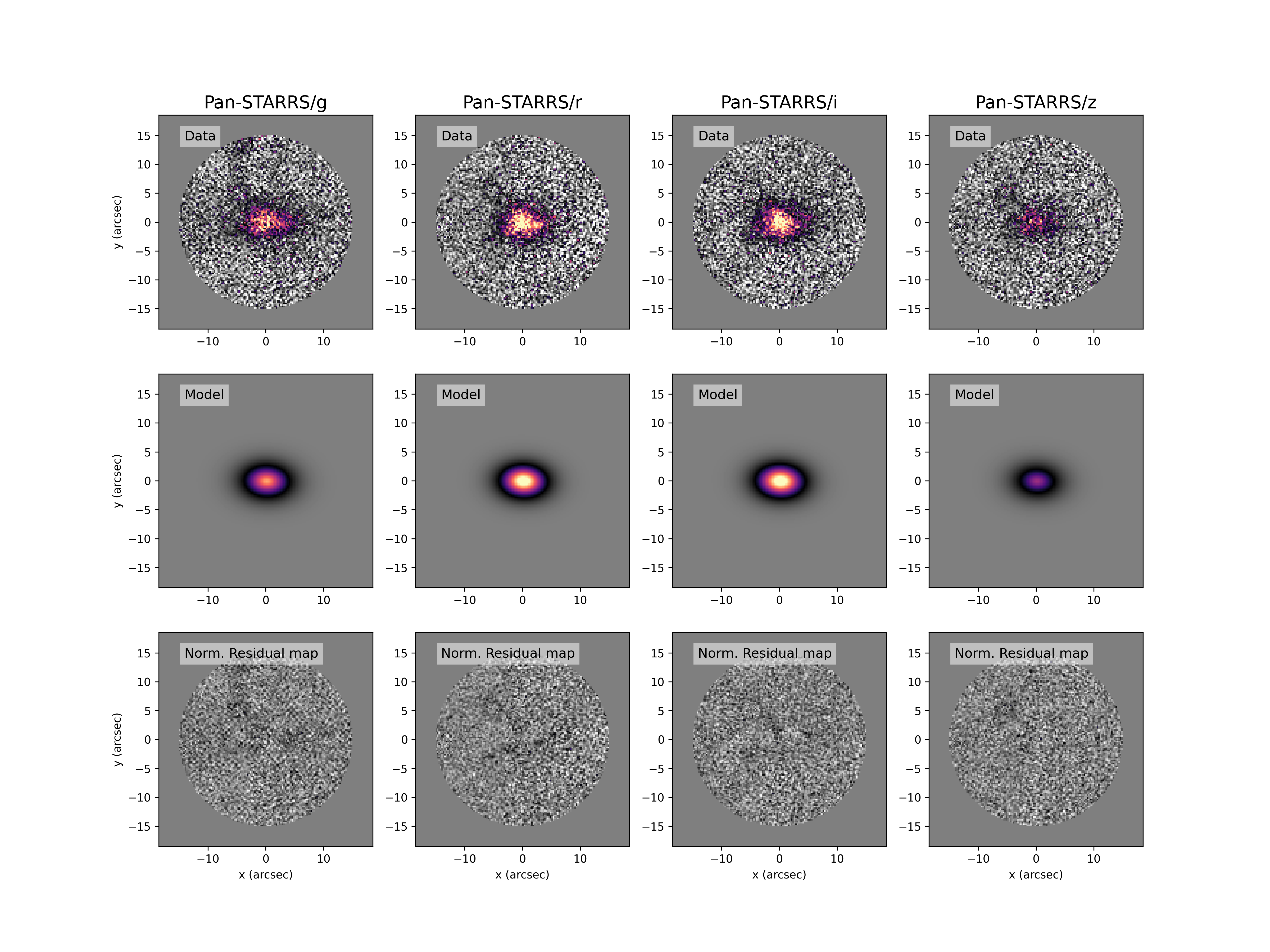
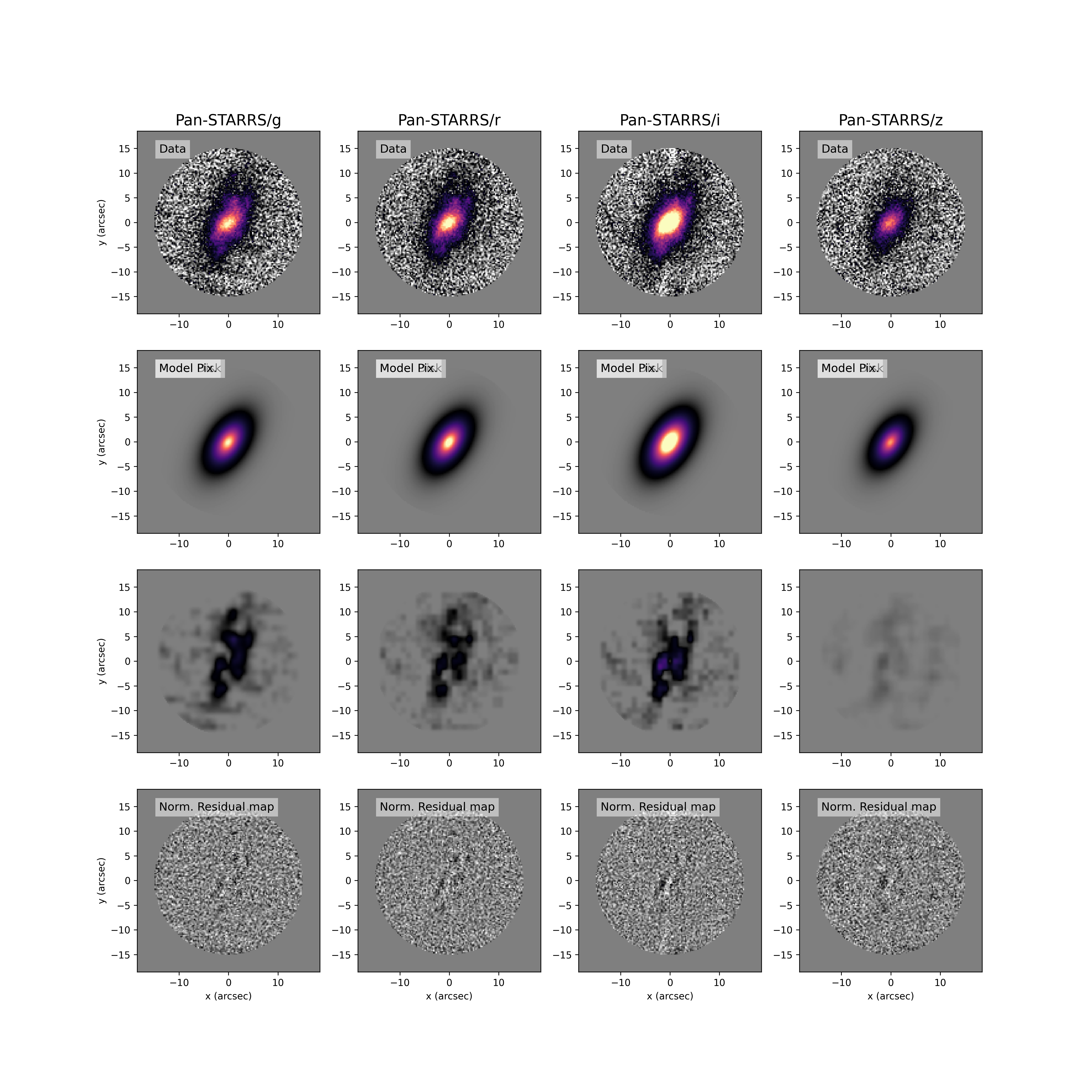
Figure 16: Surface brightness fit on the hosts of SNe 2010mc (left) and 2024hpj (right). For each band, the data, model, and residuals are shown. For SN 2024hpj, separate models for the exponential disc (second row) and spiral arms (third row) are shown.

To apply a uniform treatment to all hosts, we decided on a simple model composed of an exponential star formation history (SFH, Carnall et al. 2018) and a Calzetti dust extinction law (Calzetti et al. 1994). The redshift was assumed to be the same as the one measured on the SNe. In total, we had five free parameters: the time since the beginning of the star-formation ($\rm Age_{exp}$) and its timescale ($\rm\tau_{exp}$), the dust extinction in V-band magnitudes ($A_{\rm V}$), the metallicity relative to the solar value ($Z_{\rm exp}/Z_{\odot}$), and integrated formed stellar mass across time $\log_{10}(M_{\rm exp}/M_{\odot})$. To quantify whether the hosts are star-forming or quiescent, we compare them with the star-formation main sequence (SFMS) obtained by Boselli et al. (2023) for a sample of H I-normal galaxies in the Virgo cluster spanning stellar masses within $10^{7}<M_{*}<10^{11}$. The SFMS best fitting parameters are a slope of $0.92\pm 0.02$, an intercept of $-1.57\pm 0.53$ computed at the reference mass of $10^{8.451}$, and an intrinsic scatter of $0.42$ dex. The SED fits are shown for each host galaxy in Fig. 17.

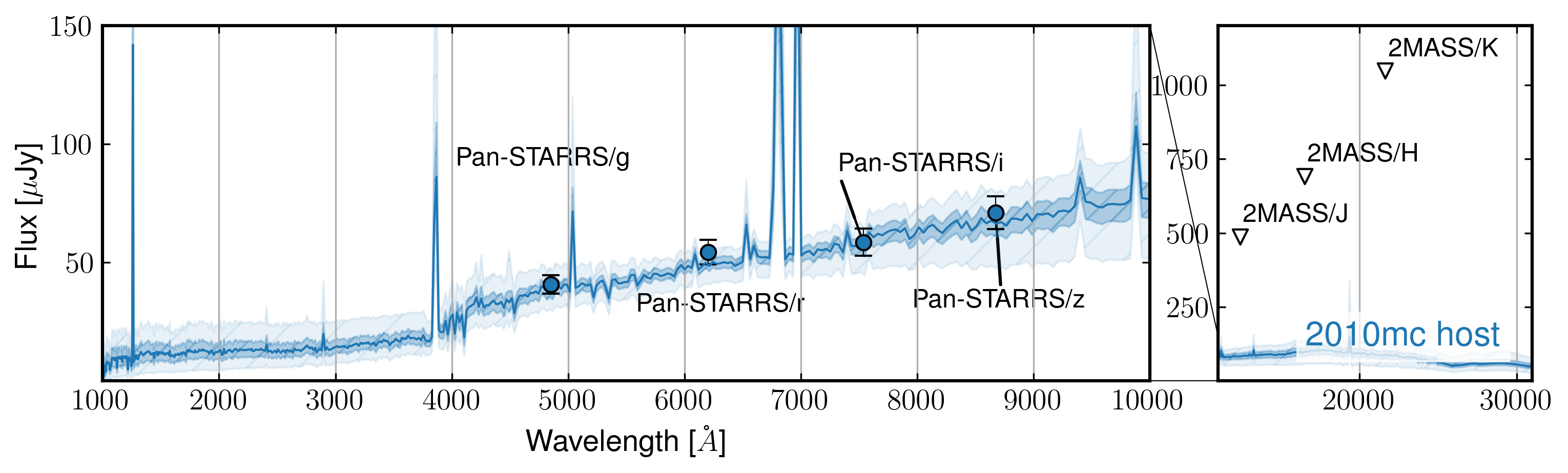
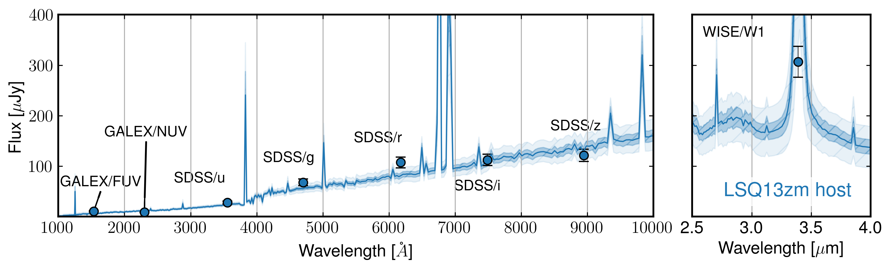
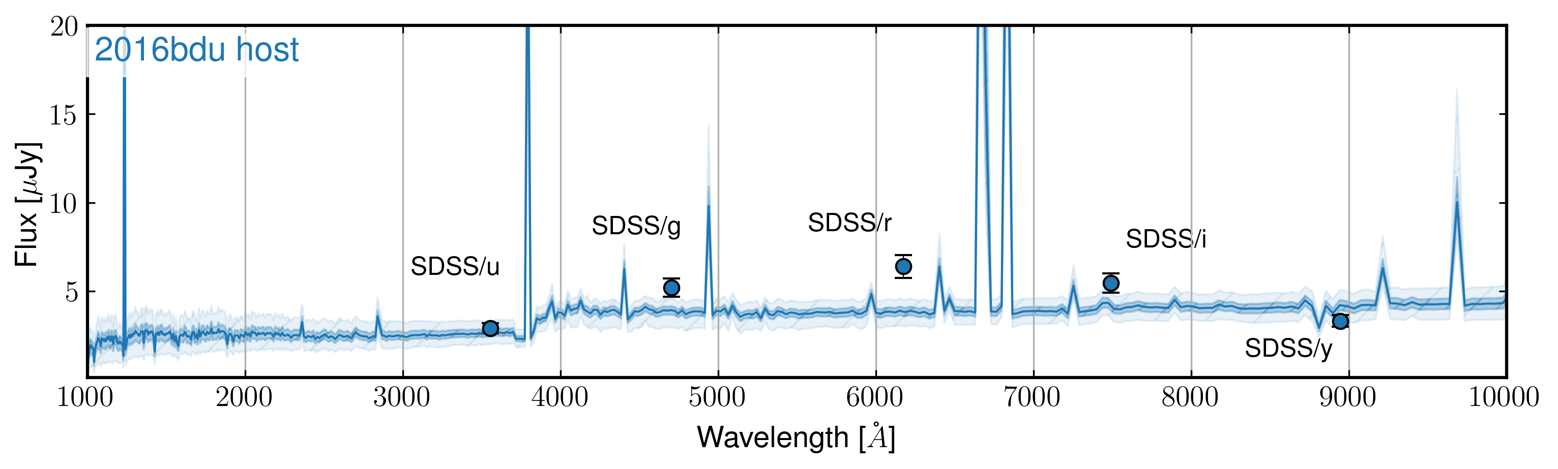
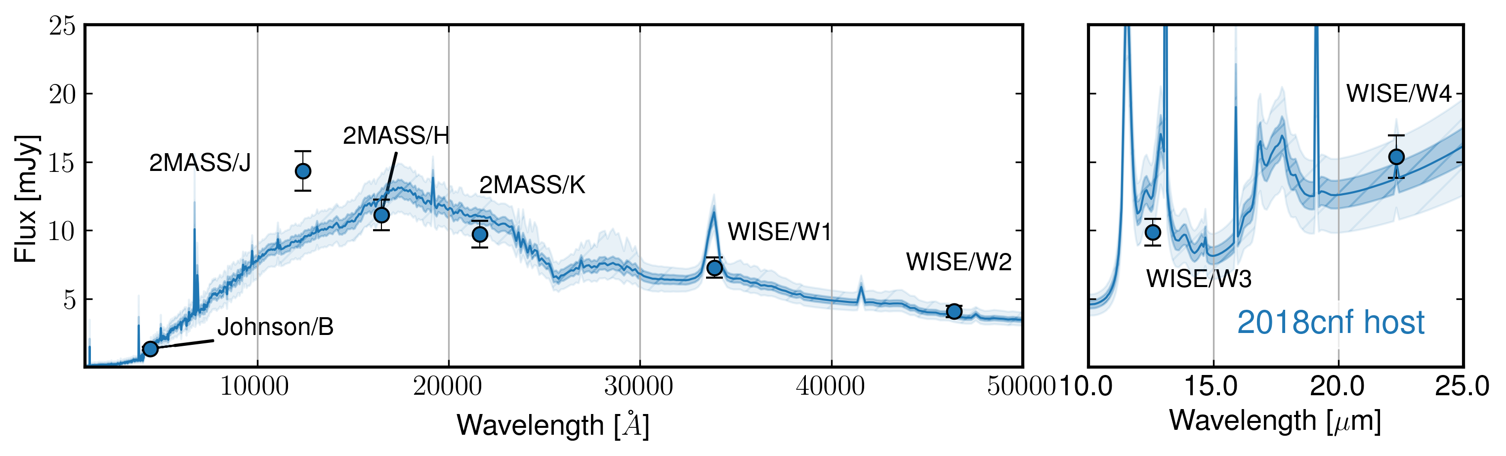
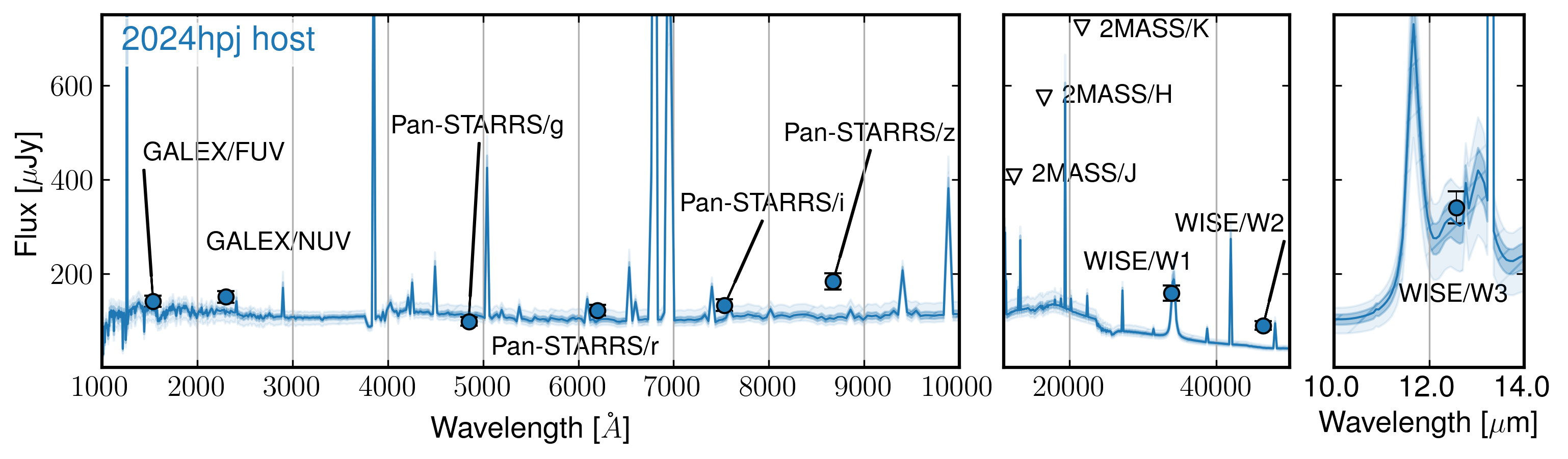
Figure 17: SED fit of the host galaxies of (from top to bottom) SNe 2010mc, LSQ13zm, 2016bdu, 2018cnf, and 2024hpj.

In the following, we summarise the main results for each host galaxy:

2010mc host: we used the Pan-STARRS $g,r,i,z$ flux densities measured with the surface brightness fitting and upper limits for the 2MASS $J,H,K$. The host appears to be a $10^{8.15}$ M_⊙ dwarf galaxy with a very low dust content ($A_{\rm V}<0.81$ at the $95^{\rm th}$ percentile). The galaxy sits on the upper part of the main sequence with a $\log_{10}(SFR)_{\rm SED}-\log_{10}(SFR)_{\rm MS}=0.49$, hence being a normal star-forming galaxy.

LSQ13zm host: we used the GALEX $FUV$ and $NUV$, SDSS $u,g,r,i,z$, and WISE $W1$ flux densities available from NED. The host appears to be a $10^{8.14}$ M_⊙ dwarf galaxy with a high dust content ($A_{\rm V}=1.45^{+0.13}_{-0.19}$ at the $95^{\rm th}$ percentile). The galaxy sits well above the main sequence with a $\log_{10}(SFR)_{\rm SED}-\log_{10}(SFR)_{\rm MS}=1.29$ ($\sim\times 3$ the intrinsic scatter), consistent with the galaxy experiencing a starbursting phase.

2016bdu host: we used the SDSS $u,g,r,i,z$ flux densities available from NED. The host appears to be a very low-mass $10^{5.75}$ M_⊙ dwarf galaxy with a low dust content ($A_{\rm V}<0.41$ at the $95^{\rm th}$ percentile). The galaxy sits well above the main sequence with a $\log_{10}(SFR)_{\rm SED}-\log_{10}(SFR)_{\rm MS}=1.26$ ($\sim\times 3$ the intrinsic scatter), consistent with the galaxy experiencing a starbursting phase.

2018cnf host: we used the Johnson $B$, 2MASS $J,H,K$, and WISE $W1,W2,W3,W4$ flux densities available from NED. The host is the most massive galaxy on which we performed the fit, with a mass of $10^{10.19}$ M_⊙. The metallicity is unconstrained, given the available photometry. The galaxy sits slightly below the main sequence with a $\log_{10}(SFR)_{\rm SED}-\log_{10}(SFR)_{\rm MS}=-0.12$. Nevertheless, given the intrinsic scatter of 0.42 dex, the host of SN 2018cnf is consistent with being a main sequence galaxy.

2024hpj host: we used the GALEX $FUV$ and $NUV$ and WISE $W1,W2,W3$ flux densities available from NED and the Pan-STARRS $g,r,i,z$ flux densities measured with the surface brightness fitting. The host appears to be a $10^{7.47}$ M_⊙ dwarf galaxy with a very low dust content ($A_{\rm V}=0.10\pm 0.01$), while the $\tau_{\rm exp}$ in unconstrained. The posteriors of the metallicity seem to suggest very high values, with $Z_{\rm exp}/Z_{\odot}>1.$ The galaxy sits well above the main sequence with a $\log_{10}(SFR)_{\rm SED}-\log_{10}(SFR)_{\rm MS}=1.99$ ($\sim\times 5$ the intrinsic scatter), consistent with the galaxy experiencing a strong starbursting phase.