Optically Controlled Skyrmion Number Current

Abstract

We propose a theoretical mechanism to control the motion of magnetic Skyrmions through the generation of a Skyrmion number current. This current is induced and tuned by an explicitly time-dependent Hamiltonian that includes a Zeeman term arising from the interaction between the spin system and circularly polarized light. To capture the effect, we apply a first-order perturbation method to the Landau–Lifshitz–Gilbert (LLG) equation, using a breathing Skyrmion ansatz based on the Belavin–Polyakov profile. This approach reveals that the time-dependent deformation of the Skyrmion boundary produces an anisotropic breathing mode, which in turn generates a nonzero Skyrmion number current. The resulting dynamics in momentum space form a limit cycle, whose characteristics depend solely on the external magnetic field amplitude, the Heisenberg exchange coupling, and the Gilbert damping constant. Our formulation not only clarifies the topological origin of optically driven Skyrmion motion but also points to Skyrmion number currents as a low-dissipation alternative to electric currents for efficient Skyrmion control.

1 Introduction

The study of the equations of motion (EOM) of local defects in magnetic systems is a central topic in spintronics, as it underpins strategies for controlling magnetic states [26]. Among these defects, a particularly important class is the topological defects, whose configurations are protected from the vacuum by topological stabilisation, which makes them more robust against perturbations. This protection originates from the conservation of a topological charge associated with the nontrivial topology of the spin texture in real space [12, 11, 7, 24]. It is known that the EOM of such defects are influenced by both the surrounding electric current and the external magnetic field profile, which can be exploited to control their motion [22, 25, 3]. However, scattering between the electric current and the lattice leads to significant energy dissipation, reducing the efficiency of electric current-based control methods [4, 5, 6].

One of the physically interesting topological defects in two- and three-dimensional systems is the Skyrmion, a quasiparticle which was first proposed in models of strongly interacting particles [19, 20, 15, 16]. The Skyrmion solutions are then found in the models of two-dimensional magnetic systems, which were considered as metastable states [17], but later it was found that such solutions can be stabilized by the competition between magnetostatic energy and anti-symmetric exchange interaction [2, 1].

A Skyrmion possesses a topological invariant known as the Skyrmion number. This Skyrmion number is a conserved charge which has its conserved current. This current related to the SKyrmion number is simply called the Skyrmion number current. The influence of the skyrmion number current on the equations of motion of magnetic skyrmions has been investigated theoretically, and it is known to compete with the effect of the electric current [14, 21]. In the absence of an electric current, the skyrmion’s velocity is therefore strongly governed by the skyrmion number current. Since the skyrmion number depends on $\partial_{t}\mathbf{n}$, this current can be controlled by adjusting the dynamics of $\mathbf{n}$, for example, through the application of an external magnetic field [6, 8, 23]. This approach enables indirect control of the skyrmion trajectory via time-dependent external fields acting through the skyrmion number current. Compared to electric-current-based methods, skyrmion-number-current-based control offers a wider range of possible mechanisms, with the potential for higher energy efficiency.

2 Understanding Skyrmion Number Current

The important quantity describing the magnetic Skyrmion is the Skyrmion number, or the topological charge of the magnetic Skyrmion, defined by

$$Q=\frac{1}{4\pi}\int\textbf{n}\cdot\left(\partial_{x}\textbf{n}\times\partial_{y}\textbf{n}\right)\penalty 10000\ d^{2}x.$$ (1)

Using this definition of Skyrmion number, we can define the Skyrmion number density and current,

$$q\equiv\frac{1}{4\pi}\textbf{n}\left(\partial_{x}\textbf{n}\times\partial_{y}\textbf{n}\right),\penalty 10000\ \penalty 10000\ \penalty 10000\ \textbf{j}\equiv\frac{1}{4\pi}\begin{bmatrix}-\textbf{n}\cdot\left(\partial_{t}\textbf{n}\times\partial_{y}\textbf{n}\right)\\ \textbf{n}\cdot\left(\partial_{t}\textbf{n}\times\partial_{x}\textbf{n}\right)\end{bmatrix}.$$ (2)

The Skyrmion number current defined above is chosen such that we have a continuity equation for Skyrmion number, namely

$$\partial_{t}q+\nabla\cdot\textbf{j}=0.$$ (3)

This implies that the Skyrmion number is preserved, by definition.

The generalized Skyrme field, $\phi$, on arbitrary dimensional flat base space can be defined as a map from the $d$ dimensional Euclidean space, $\mathbb{R}^{d}$ to a $d$ dimensional sphere, $S^{d}$. This implies that the generalized Skyrme model belongs to the non-linear sigma models with special topological property, coming from the fact that $\phi:\mathbb{R}^{d}\rightarrow S^{d}$ has homotopy group $\pi_{d}(S^{d})$.

The conservation equation (3) coincides with the Faraday’s equation of emergent electromagnetism generated by the Skyrmion, namely

$$\partial_{t}\textbf{b}+\nabla\times\textbf{e}=0,$$ (4)

where the emergent magnetic and electric fields are given by

$$\textbf{b}=\textbf{n}\cdot\left(\partial_{x}\textbf{n}\times\partial_{y}\textbf{n}\right)\hat{z},\penalty 10000\ \penalty 10000\ \penalty 10000\ \textbf{e}=\textbf{n}\cdot\left(\partial_{x}\textbf{n}\times\partial_{t}\textbf{n}\right)\hat{x}+\textbf{n}\cdot\left(\partial_{y}\textbf{n}\times\partial_{t}\textbf{n}\right)\hat{y}.$$ (5)

This emergent Faraday’s law has been experimentally confirmed [10, 13, 18] which implies that the Skyrmion number is indeed a conserved charge.

3 Equation of Motion of Magnetic Skyrmion

We propose that a significant effect of topology on the Skyrmion motion can be observed in the following setup for an isolated Skyrmion in a medium that is free from electric current. Let us consider a magnetic system with Hamiltonian density $H\equiv H(\textbf{n},\partial_{k}\textbf{n},\textbf{r})$. $\textbf{n}\equiv\textbf{n}(t,\textbf{r})$ is spin orientation at position r and time $t$. The dynamics of the spins inside this system is assumed to obey the Landau-Lifshitz-Gilbert (LLG) equation, given by

$$\partial_{t}\textbf{n}=\gamma\left(\textbf{n}\times\frac{\delta H}{\delta\textbf{n}}+\alpha\textbf{n}\times\partial_{t}\textbf{n}\right).$$ (6)

If we apply translation to the coordinate system with respect to vector $\textbf{R}(t)=(X(t),Y(t))$, $\textbf{n}(t,\textbf{r})\rightarrow\textbf{n}(t,\textbf{r}-\textbf{R}(t))$, then the time derivative of n becomes

$$\partial_{t}\textbf{n}\rightarrow\partial_{t}\textbf{n}-(\partial_{t}\textbf{R}\cdot\nabla)\textbf{n}.$$ (7)

Going back to the LLG equation, taking the cross product of each sides with n gives us

$$\textbf{n}\times\partial_{t}\textbf{n}-\textbf{n}\times(\partial_{t}\textbf{R}\cdot\nabla)\textbf{n}=\gamma\left[\textbf{n}\left(\textbf{n}\cdot\frac{\delta H}{\delta\textbf{n}}\right)-\frac{\delta H}{\delta\textbf{n}}-\alpha\partial_{t}\textbf{n}+\alpha(\partial_{t}\textbf{R}\cdot\nabla)\textbf{n}\right].$$ (8)

We can remove the first term on the RHS above dot-multiplying the equations with $\partial_{i}\textbf{n}$, such that

$$\gamma\partial_{i}\textbf{n}\cdot\frac{\delta H}{\delta\textbf{n}}-\gamma\alpha(\partial_{t}\textbf{R}\cdot\nabla)\textbf{n}\cdot\partial_{i}\textbf{n}+n\cdot\left((\partial_{t}\textbf{R}\cdot\nabla)\textbf{n}\times\partial_{i}\textbf{n}\right)=n\cdot\left(\partial_{t}\textbf{n}\times\partial_{i}\textbf{n}\right)-\gamma\alpha\partial_{i}\textbf{n}\cdot\partial_{t}\textbf{n}.$$ (9)

As a result, we have two equations for $i=x,y$, namely

$$\gamma\begin{bmatrix}\partial_{x}\textbf{n}\cdot\frac{\delta H}{\delta\textbf{n}}\\ \partial_{y}\textbf{n}\cdot\frac{\delta H}{\delta\textbf{n}}\end{bmatrix}-\gamma\alpha\mathcal{D}\cdot\partial_{t}\textbf{R}+4\pi q\hat{z}\times\partial_{t}\textbf{R}=-4\pi\hat{z}\times\textbf{j}-\gamma\alpha\begin{bmatrix}\partial_{t}\textbf{n}\cdot\partial_{x}\textbf{n}\\ \partial_{t}\textbf{n}\cdot\partial_{y}\textbf{n}\end{bmatrix}.$$ (10)

We define the strain tensor,

$$\mathcal{D}\equiv\begin{bmatrix}\partial_{x}\textbf{n}\cdot\partial_{x}\textbf{n}&\partial_{x}\textbf{n}\cdot\partial_{y}\textbf{n}\\ \partial_{x}\textbf{n}\cdot\partial_{y}\textbf{n}&\partial_{y}\textbf{n}\cdot\partial_{y}\textbf{n}\end{bmatrix},$$ (11)

which is a well-defined tensor satisfying $\mathcal{D}=\mathcal{J}\mathcal{J}^{T}$ where $\mathcal{J}$ is the Jacobi matrix for the map $\textbf{n}:\mathbb{R}^{2}\rightarrow S^{2}$.

We can remove the spatial dependence of the equation of motion above by integrating the equation throughout the entire plane. To do this, consider the first term above which translates into

$$\partial_{i}\textbf{n}\cdot\left(\frac{\partial H}{\partial\textbf{n}}-\frac{d}{d(\textbf{r})^{i}}\frac{\partial H}{\partial(\partial_{k}\textbf{n})}\right)=\frac{dH}{d(\textbf{r})^{i}}-\partial_{i}H,$$ (12)

by assuming that $H\equiv H(\textbf{n},\partial_{k}\textbf{n},\textbf{r})$. Here, we have neglected all the bondary terms which gives zero contribution to the functional integral. The first term in (12) is zero if we integrate it throughout the plane since it becomes a boundary integral, however, the second term is non-trivial

$$-\int\partial_{i}H((\textbf{n}(\textbf{r}-\textbf{R}),\partial_{k}\textbf{n}(\textbf{r}-\textbf{R}),\textbf{r}))d^{2}x = -\int\frac{\partial}{\partial(\textbf{r}+\textbf{R})^{i}}H((\textbf{n}(\textbf{r}),\partial_{k}\textbf{n}(\textbf{r}),\textbf{r}+\textbf{R}))d^{2}x$$ (13)

$$= -\frac{\partial}{\partial(\textbf{R})^{i}}\int H((\textbf{n}(\textbf{r}),\partial_{k}\textbf{n}(\textbf{r}),\textbf{r}+\textbf{R}))d^{2}x$$

$$= -\frac{1}{\gamma}\frac{\partial}{\partial(\textbf{R})^{i}}V(\textbf{R}).$$

Using this result and expressing the integrals of $q$, j, and $\mathcal{D}$ with

$$Q=\int q\penalty 10000\ d^{2}x,\penalty 10000\ \penalty 10000\ \penalty 10000\ \textbf{J}_{Q}=\int\textbf{j}\penalty 10000\ d^{2}x,\penalty 10000\ \penalty 10000\ \penalty 10000\ \mathcal{G}=\gamma\alpha\int\mathcal{D}\penalty 10000\ d^{2}x,$$ (14)

such that,

$$\nabla_{\textbf{R}}V(\textbf{R})+\mathcal{G}\cdot\partial_{t}\textbf{R}-4\pi Q\hat{z}\times\partial_{t}\textbf{R}=4\pi\hat{z}\times\textbf{J}_{Q}+\gamma\alpha\int\begin{bmatrix}\partial_{t}\textbf{n}\cdot\partial_{x}\textbf{n}\\ \partial_{t}\textbf{n}\cdot\partial_{y}\textbf{n}\end{bmatrix}d^{2}x.$$ (15)

As implied by the equation of motion above, the Skyrmion number current naturally show up in the LLG equation when the Skyrmion profile is allowed evolve with respect to time. The effect of the Skyrmion number current in magnetic Skyrmion dynamics has been known for decades [14, 9]. The contribution of the Skyrmion number current behaves similarly with the electric current contribution, which shows up in the LLG equation when the spin transfer torque is also considered. This provides us with an alternative current-free mechanism for Skyrmion control [3]. It is also known that this Skyrmion number current is proportional to the electric current when the emergent electromagnetic field is non-dynamical and the Skyrmion is in steady motion [21].

4 Skyrmion Motion with Nearly Homogenous Hamiltonian

Since the Skyrmion number current could influence the motion of Skyrmion similar to the electric current, we can control the Skyrmion’s trajectory by manipulating its time-dependence through a time-dependent Hamiltonian. Resulting induced Skyrmion number current which drives the motion of the Skyrmion. For a nearly homogenous Hamiltonian $\partial_{i}H\approx 0$, we have $V(\textbf{R})\simeq V_{0}$, such that the trajectory of the Skyrmion is governed by

$$\mathcal{G}\cdot\partial_{t}\textbf{R}-4\pi Q\hat{z}\times\left(\partial_{t}\textbf{R}+\frac{\textbf{J}_{Q}}{Q}\right)=\gamma\alpha\int\begin{bmatrix}\partial_{t}\textbf{n}\cdot\partial_{x}\textbf{n}\\ \partial_{t}\textbf{n}\cdot\partial_{y}\textbf{n}\end{bmatrix}d^{2}x.$$ (16)

In order to solve the equation above for $\textbf{R}(t)$ we first need the expression for the Skyrmion profile which depends on the Hamiltonian of the system.

4.1 Isotropic Skyrmion

Let us start the study of the Skyrmion trajectory governed by (16), with a simple isotropic Skyrmion with time dependence. The form of time-dependency is chosen so that the Skyrmion maintains its shape throughout the evolution.

4.1.1 Setup

For this case, we assume that the Skyrmion number current is directed to the $\hat{x}$ axes without any loss of generality. the Skyrmion is assumed to be anisotropic such that $\textbf{J}_{Q}\cdot\hat{y}=0$. This can be achieved if

$$\textbf{n}\cdot(\partial_{t}\textbf{n}\times\partial_{x}\textbf{n})=0.$$ (17)

One of the realistic mechanism to generate this type of oscillating field is by applying a plane wave light directed perpendicular to the system. Let us assume the external field came from a plane wave with polarization p, $\textbf{B}(t)=B_{0}\cos(\omega t)\textbf{p}$. However, as mentioned previously, $B_{0}$ must be small enough such that $\textbf{n}_{0}$ is stable. We can find the upper bound for $B_{0}$ from the comparison between the wave’s energy and the energy dissipated by Gilbert’s damping. Let $U=\int H\penalty 10000\ d^{2}x$, be the total energy of the system, hence the rate of the energy over time is $dU/dt=\int\left[\left(\delta H/\delta\textbf{n}\right)\cdot\partial_{t}\textbf{n}+\partial_{t}H\right]d^{2}x$. We know from the LLG equation that $\partial_{t}\textbf{n}=\gamma\left[\textbf{n}\times(\delta H/\delta\textbf{n})+\alpha\gamma\textbf{n}\times\left(\textbf{n}\times(\delta H/\delta\textbf{n})\right)\right]/(1+\alpha^{2}\gamma^{2})$. Thus, we arrive at

$$\frac{dU}{dt}=\int\left[\frac{\alpha\gamma^{2}}{1+\alpha^{2}\gamma^{2}}\left(\left(\frac{\delta H}{\delta\textbf{n}}\cdot\textbf{n}\right)^{2}-\frac{\delta H}{\delta\textbf{n}}\cdot\frac{\delta H}{\delta\textbf{n}}\right)+\partial_{t}H\right]d^{2}x\penalty 10000\ .$$ (18)

This energy rate must be bounded above by zero, $dU/dt\leq 0$, which physically implies that the dissipated energy is always higher than energy supplied by the wave. We need to estimate the bound above for a single period of the wave. One possible way to satisfy the bound for $dU/dt$ is by considering a stronger bound where the integrand in (18) is bounded by zero, namely

$$\max_{t\in[0,2\pi/\omega]}\left(\frac{1+\alpha^{2}\gamma^{2}}{\alpha\gamma^{2}}\partial_{t}H-\frac{\delta H}{\delta\textbf{n}}\cdot\frac{\delta H}{\delta\textbf{n}}\right)<0\penalty 10000\ ,$$ (19)

where we have dropped the first term since it is a positive-definite term. Now, for the special case with Heisenberg Hamiltonian perturbed by external magnetic field $\textbf{B}(t)$, $H=J\partial_{i}\textbf{n}\cdot\partial_{i}\textbf{n}-\textbf{B}(t)\cdot\textbf{n}$, we have effective magnetic field $-\delta H/\delta\textbf{n}=2J\nabla^{2}\textbf{n}+\textbf{B}(t)$. As such, we can recast the inequality above into

$$\frac{1+\alpha^{2}\gamma^{2}}{\alpha\gamma^{2}}\max_{t\in[0,2\pi/\omega]}\partial_{t}H<\min_{t\in[0,2\pi/\omega]}\frac{\delta H}{\delta\textbf{n}}\cdot\frac{\delta H}{\delta\textbf{n}}$$ (20)

$$\Rightarrow \frac{1+\alpha^{2}\gamma^{2}}{\alpha\gamma^{2}}\max_{t\in[0,2\pi/\omega]}\left(-\partial_{t}\textbf{B}(t)\cdot\textbf{n}\right)<\min_{t\in[0,2\pi/\omega]}\|2J\nabla^{2}\textbf{n}+\textbf{B}(t)\|.$$

This inequality can be estimated using the unperturbed Skyrmion texture that solves $\textbf{n}_{0}\times\nabla^{2}\textbf{n}_{0}=0$ such that

$$\frac{1+\alpha^{2}\gamma^{2}}{\alpha\gamma^{2}}\omega B_{0}\penalty 10000\ \textbf{p}\cdot\textbf{n}_{0}<\|2J\nabla^{2}\textbf{n}_{0}\|^{2}.$$ (21)

The unperturbed solution $\textbf{n}_{0}$ is well-known as the Belavin-Polyakov (BP) solution [17], that is given by $\textbf{n}_{0}=(2\lambda(x\cos\gamma-y\sin\gamma),\penalty 10000\ 2\lambda(x\sin\gamma+y\cos\gamma),\penalty 10000\ \lambda^{2}-r^{2})/(\lambda^{2}+r^{2})$, where $r^{2}=x^{2}+y^{2}$, $\lambda$ is the Skyrmion radius, and $\gamma$ is the Skyrmion helicity. The LHS of (21) is $(x,y)$ dependent through $\textbf{p}\cdot\textbf{n}_{0}$ that is maximized at $r=\lambda$. Let $\nu$ be the polarization angle such that $\textbf{p}=(\cos\nu,\sin\nu)$, then at $r=\lambda$ we have $\textbf{p}\cdot\textbf{n}_{0}=\cos(\varphi+\nu+\gamma)$ where $\varphi=\tan^{-1}(y/x)$. As such, the maximum value of $\textbf{p}\cdot\textbf{n}_{0}$ is equal to one. On the other hand, the RHS of (21) is $(x,y)$ dependent through $\|\nabla^{2}\textbf{n}_{0}\|^{2}$. If we substitute the BP solution into this norm, we have $\|\nabla^{2}\textbf{n}_{0}\|^{2}=64\lambda^{4}/(\lambda^{2}+r^{2})^{4}$ that is evaluated to $4/\lambda^{4}$ at $r=\lambda$. As a result, the estimated upper bound for $B_{0}$ is given by

$$\omega B_{0}<\frac{\alpha\gamma^{2}}{1+\alpha^{2}\gamma^{2}}\frac{16J^{2}}{\lambda^{4}}.$$ (22)

Beyond this value of $B_{0}$, the Zeeman effect will become significant compared to the exchange interaction and the stability of the solution $\textbf{n}(t,\textbf{r})$ is not guaranteed.

To estimate the form of time dependence of $\textbf{B}(t)$, we can substitute the $\partial_{t}\textbf{n}$ from LLG equation to (17), to obtain

$$\textbf{n}\cdot(\left[\textbf{n}\times(\delta H/\delta\textbf{n})+\alpha\gamma\textbf{n}\times\left(\textbf{n}\times(\delta H/\delta\textbf{n})\right)\right]\times\partial_{x}\textbf{n})=0$$ (23)

$$\Rightarrow \textbf{n}\cdot\left[-\partial_{x}\textbf{n}\left(\textbf{n}\cdot\frac{\partial H}{\partial\textbf{n}}\right)+\alpha\gamma\left(\textbf{n}\left(\textbf{n}\cdot\frac{\partial H}{\partial\textbf{n}}\right)-\frac{\partial H}{\partial\textbf{n}}\right)\times\partial_{x}\textbf{n}\right]=0$$

$$\Rightarrow \partial_{x}\textbf{n}\cdot\left(\textbf{n}\times\frac{\partial H}{\partial\textbf{n}}\right)=0.$$

4.1.2 Skyrmion Texture and Trajectory

Suppose that $\textbf{n}=\left(\sin\Theta\cos\Phi,\sin\Theta\sin\Phi,\cos\Theta\right)$. Then condition (17) implies that $\partial_{x}\Phi\partial_{t}\Theta-\partial_{x}\Theta\partial_{t}\Phi=0$, which is satisfied by applying the Galilean transformation of the $x$ axes in static solution, satisfying $(\Theta(x,y),\Phi(x,y))\rightarrow(\Theta(x-\eta t,y),\Phi(x-\eta t,y))$. Let us consider the transformed $Q=1$ Belavin-Polyakov Skyrmion solution as follows,

$$\textbf{n}=\begin{bmatrix}2\lambda_{0}\left((x-\eta t)\cos\varphi_{0}-y\sin\varphi_{0}\right)/(\lambda^{2}_{0}+(x-\eta t)^{2}+y^{2})\\ 2\lambda_{0}\left((x-\eta t)\sin\varphi_{0}+y\cos\varphi_{0}\right)/(\lambda^{2}_{0}+(x-\eta t)^{2}+y^{2})\\ (\lambda^{2}_{0}-(x-\eta t)^{2}-y^{2})/(\lambda^{2}_{0}+(x-\eta t)^{2}+y^{2}).\end{bmatrix}$$ (24)

This solution is an axially symmetric Skyrmion with radius $\lambda_{0}$ and helicity $\varphi_{0}$ which moves in the positive $\hat{x}$ direction with speed $\eta$. Thus, the non-zero $\hat{x}$ component of the Skyrmion number current is generated by the Skyrmion moving in the same direction. According to this description, the velocity vector of this solution is given by $\partial_{t}\textbf{R}=(0,\eta)$. Substituting this velocity and the profile (24) back into Eq. (16), the equation become trivial. This implies that our description Skyrmion trajectory above is consistent with the equation of motion.

4.2 Breathing Skyrmion

Now, let us consider a more interesting case where the Skyrmion’s profile is influenced by external field. The external field is time dependent, which in turn generates a time dependency on the skyrmion radius and helicity. This results in a Skyrmion number current whose dynamics is non-trivial.

4.2.1 Setup

We consider a case where the magnetic field is assumed to be generated by a circularly polarized plane wave such that $\textbf{B}(t)=B_{0}(\cos(\omega t),\sin(\omega t))=B_{0}\textbf{p}(t)$. Similar to the previous case, we have the following inequality

$$\frac{1+\alpha^{2}\gamma^{2}}{\alpha\gamma^{2}}B_{0}\max_{t\in[0,2\pi/\omega]}\left(-\partial_{t}\textbf{p}(t)\cdot\textbf{n}_{0}\right)<\|2J\nabla^{2}\textbf{n}_{0}\|^{2}$$ (25)

$$\Rightarrow \omega B_{0}<\frac{\alpha\gamma^{2}}{1+\alpha^{2}\gamma^{2}}\frac{16J^{2}}{\lambda_{0}^{4}},$$

that is the same upper bound we found for plane wave in the previous case.

4.2.2 Skyrmion Texture

For this case, we use the perturbation method on the Skyrmion profile of Belavin-Polyakov (BP) type [17],

$$\textbf{n}=\begin{bmatrix}2r\lambda(t,\varphi)\cos\left(\Phi(t,\varphi)\right)/(\lambda^{2}(t,\varphi)+r^{2})\\ 2r\lambda(t,\varphi)\sin\left(\Phi(t,\varphi)\right)/(\lambda^{2}(t,\varphi)+r^{2})\\ (\lambda^{2}(t,\varphi)-r^{2})/(\lambda^{2}(t,\varphi)+r^{2})\end{bmatrix},$$ (26)

and the Hamiltonian density is assumed to obey the Heisenberg model

$$H=J\partial_{i}\textbf{n}\cdot\partial_{i}\textbf{n}-\textbf{B}(t)\cdot\textbf{n},$$ (27)

where $J$ is the Heisenberg coupling constant. Within this choice of Skyrmion profile, the set of points $r=\lambda$ is the boundary of the Skyrmion where $\textbf{n}\cdot\hat{z}=0$. The corresponding LLG equation governing the Skyrmion profile is then given by,

$$\partial_{t}\textbf{n}=-\gamma\penalty 10000\ \textbf{n}\times\left[\epsilon\textbf{B}(t)+2J\nabla^{2}\textbf{n}\right]+\alpha\gamma\penalty 10000\ \textbf{n}\times\partial_{t}\textbf{n}.$$ (28)

Here the magnetic field is considered as the perturbation from the Heisenberg Hamiltonian, whose unperturbed solution satisfies $\textbf{n}_{0}\times\nabla^{2}\textbf{n}_{0}=0$, and $\epsilon$ is a perturbation parameter.

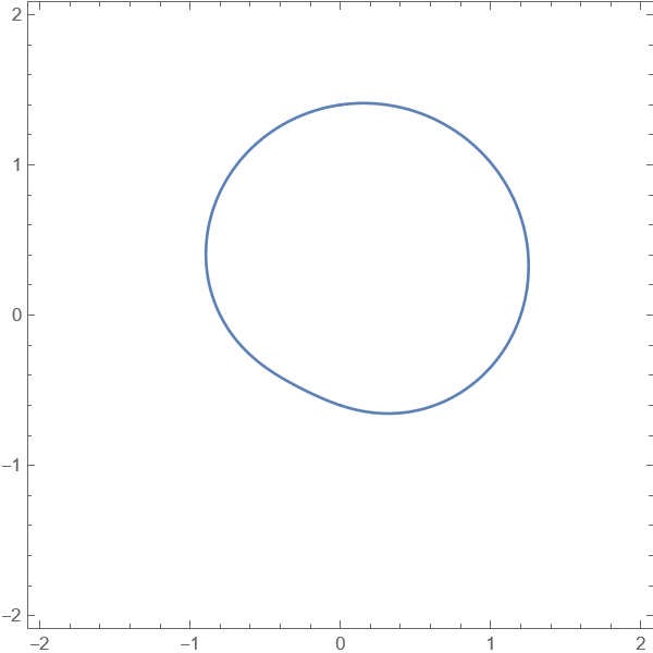
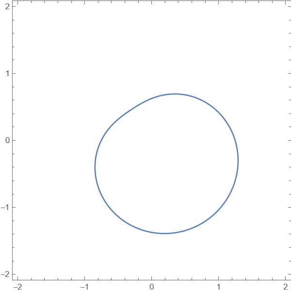
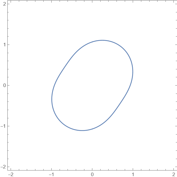
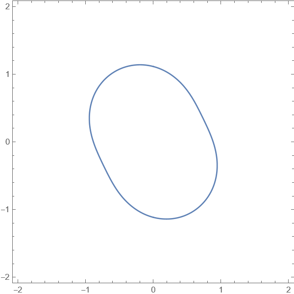
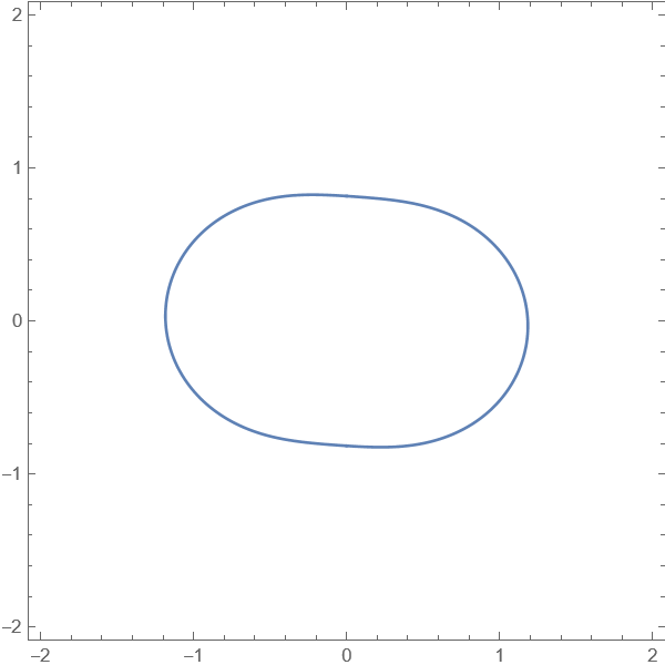
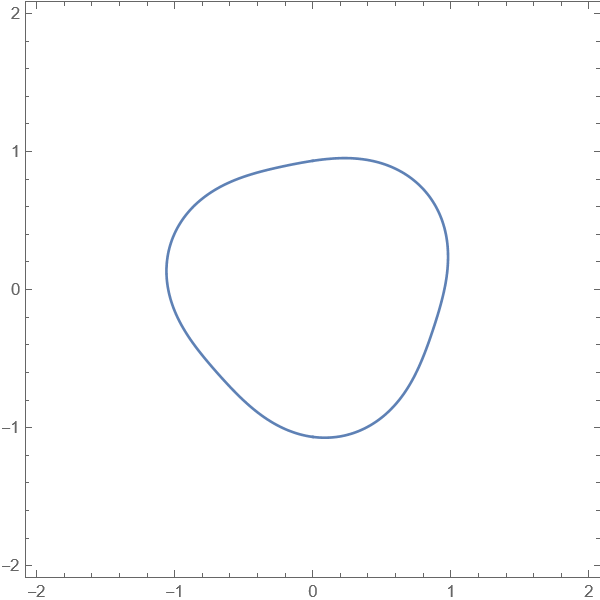
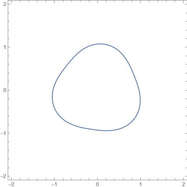
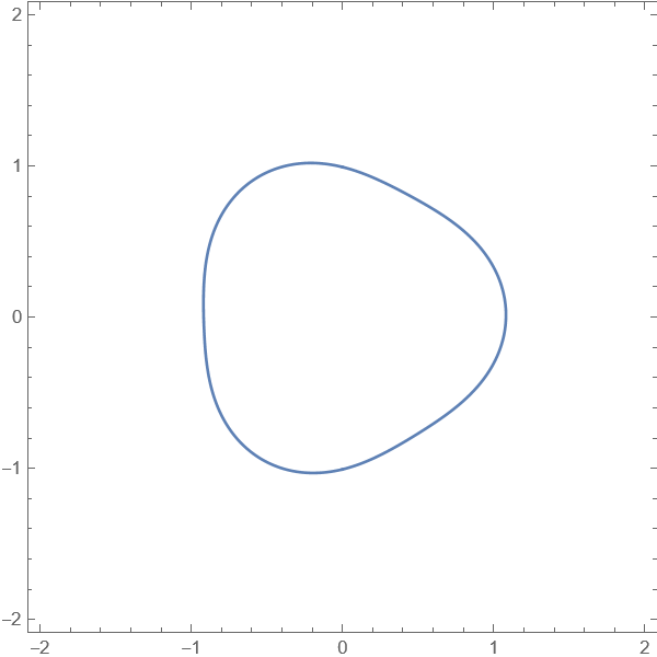
Figure 1: Boundary of the Skyrmions, $\hat{z}\cdot\textbf{n}(t,\textbf{x})=0$, with $Q=1,2,3$ with $\alpha\gamma=\eta_{1}=\eta_{2}=1$ for $\omega t=0,2\pi/3,4\pi/3$.

Let the perturbed $\lambda$ and $\Phi$ be

$$\lambda(t,\varphi)=\lambda_{0}+\sum_{k=1}^{\infty}\epsilon^{k}\tilde{\lambda}_{k}(t,\varphi),\penalty 10000\ \penalty 10000\ \penalty 10000\ \Phi(t,\varphi)=Q\varphi+\varphi_{0}+\sum_{k=1}^{\infty}\epsilon^{k}\tilde{\Phi}_{k}(t,\varphi).$$ (29)

Up to first order of $\epsilon$, the equations for $\tilde{\lambda}_{1}$ and $\tilde{\Phi}_{1}$ at the boundary of the Skyrmion are

$$\partial_{t}\tilde{\Phi}_{1}+\alpha\gamma\frac{\partial_{t}\tilde{\lambda}_{1}}{\lambda_{0}}-2\frac{\gamma J}{\lambda_{0}^{2}}\frac{\partial_{\varphi}^{2}\tilde{\lambda}_{1}}{\lambda_{0}}+2(1-Q^{2})\frac{\gamma J}{\lambda_{0}^{2}}\frac{\tilde{\lambda}_{1}}{\lambda_{0}} = 0$$ (30)

$$\frac{\partial_{t}\tilde{\lambda}_{1}}{\lambda_{0}}-\gamma B_{0}\sin\left(Q\varphi+\varphi_{0}-\omega t\right)-\alpha\gamma\partial_{t}\tilde{\Phi}_{1}+2\frac{\gamma J}{\lambda_{0}^{2}}\partial_{\varphi}^{2}\tilde{\Phi}_{1} = 0.$$ (31)

Both $\tilde{\lambda}_{1}$ and $\tilde{\Phi}_{1}$ must be periodic for $\varphi\rightarrow\varphi+2\pi$. The homogenous part of (30-31) is diffusive, hence the homogenous solutions are suppressed at the steady state limit. At steady state, the non-homogenous solution should behave like the driving term controlled by $B_{0}$. As such, the solutions are $\tilde{\lambda}_{1}/\lambda_{0}=A^{1}_{\lambda}\cos\left(Q\varphi+\varphi_{0}-\omega t\right)+A^{2}_{\lambda}\sin\left(Q\varphi+\varphi_{0}-\omega t\right)$ and $\tilde{\Phi}_{1}=A^{1}_{\Phi}\cos\left(Q\varphi+\varphi_{0}-\omega t\right)+A^{2}_{\Phi}\sin\left(Q\varphi+\varphi_{0}-\omega t\right)$. Substituting these solutions to (30) and (31) gives us

$$0 = \left[\omega A^{1}_{\Phi}+\alpha\gamma\omega A^{1}_{\lambda}+2\frac{\gamma J}{\lambda_{0}^{2}}A^{2}_{\lambda}\right]\sin\left(Q\varphi+\varphi_{0}-\omega t\right)$$ (32)

$$+\left[-\omega A^{2}_{\Phi}-\alpha\gamma\omega A^{2}_{\lambda}+2\frac{\gamma J}{\lambda_{0}^{2}}A^{1}_{\lambda}\right]\cos\left(Q\varphi+\varphi_{0}-\omega t\right),$$

$$0 = \left[\omega A^{1}_{\lambda}-\gamma B_{0}-\alpha\gamma\omega A^{1}_{\Phi}-2\frac{\gamma J}{\lambda_{0}^{2}}Q^{2}A^{2}_{\Phi}\right]\sin\left(Q\varphi+\varphi_{0}-\omega t\right)$$ (33)

$$+\left[-\omega A^{2}_{\lambda}+\alpha\gamma\omega A^{2}_{\Phi}-2\frac{\gamma J}{\lambda_{0}^{2}}Q^{2}A^{1}_{\Phi}\right]\cos\left(Q\varphi+\varphi_{0}-\omega t\right).$$

The equation above must be satisfied for all $t$. Thus, we can solve each coefficient for $(A^{1}_{\Phi},A^{2}_{\Phi},A^{1}_{\lambda},A^{2}_{\lambda})$. The solutions for these $A^{i}_{\mu}$s is then can be substituted back to $\lambda(t,\varphi)$ and $\Phi(t,\varphi)$, such that their solutions, up to first order perturbation, are given by

$$\lambda(t,\varphi) = \lambda_{0}+\lambda_{0}\frac{\eta_{1}\left(1+\alpha^{2}\gamma^{2}-\eta_{2}^{2}Q^{2}\right)}{\alpha^{4}\gamma^{4}+\left(\eta_{2}^{2}Q^{2}-1\right)^{2}+\alpha^{2}\gamma^{2}\left(\eta_{2}^{2}(1+Q^{4})+2\right)}\cos\left(Q\varphi+\varphi_{0}-\omega t\right)$$ (34)

$$+\lambda_{0}\frac{\alpha\gamma\eta_{1}\eta_{2}\left(1+Q^{2}\right)}{\alpha^{4}\gamma^{4}+\left(\eta_{2}^{2}Q^{2}-1\right)^{2}+\alpha^{2}\gamma^{2}\left(\eta_{2}^{2}(1+Q^{4})+2\right)}\sin\left(Q\varphi+\varphi_{0}-\omega t\right)\penalty 10000\ ,$$

$$\Phi(t,\varphi) = Q\varphi+\varphi_{0}-\frac{\alpha\gamma\eta_{1}\left(1+\alpha^{2}\gamma^{2}+\eta_{2}^{2}\right)}{\alpha^{4}\gamma^{4}+\left(\eta_{2}^{2}Q^{2}-1\right)^{2}+\alpha^{2}\gamma^{2}\left(\eta_{2}^{2}(1+Q^{4})+2\right)}\cos\left(Q\varphi+\varphi_{0}-\omega t\right)$$ (35)

$$+\frac{\eta_{1}\eta_{2}\left(1-\left(\alpha^{2}\gamma^{2}+\eta_{2}^{2}\right)Q^{2}\right)}{\alpha^{4}\gamma^{4}+\left(\eta_{2}^{2}Q^{2}-1\right)^{2}+\alpha^{2}\gamma^{2}\left(\eta_{2}^{2}(1+Q^{4})+2\right)}\sin\left(Q\varphi+\varphi_{0}-\omega t\right)\penalty 10000\ ,$$

where we have defined two physical parameters of the system, namely

$$\eta_{1}=\frac{\gamma B_{0}}{\omega}\penalty 10000\ ,\penalty 10000\ \penalty 10000\ \penalty 10000\ \eta_{2}=2\frac{\gamma J}{\omega\lambda_{0}^{2}}\penalty 10000\ .$$ (36)

The ratio $\eta_{1}/\eta_{2}=B_{0}\lambda_{0}^{2}/(2J)$, is the measure of the external magnetic field’s strength compared to the magnetic interaction between the spins. The upper bound for $B_{0}$ in (25), can be recast into relation between $\eta_{1}$ and $\eta_{2}$ as follows,

$$\eta_{1}<4\frac{\alpha\gamma}{1+\alpha^{2}\gamma^{2}}\eta_{2}^{2}.$$ (37)

This simpler inequality relates the dimensionless parameters, that is useful for predicting the well-behaving range in simulations of realistic model. We plot the boundary of the Skyrmion for the case of $Q=1,2,3$ in Fig. 1. We also demostrate this profile is indeed a breathing profile, specifically an anisotropic breathing profile, whose breathing phase in opposite direction is also in opposite phase (See Fig. 2).

Figure 2: The ratio between the distance from center to boundary and the unperturbed Skyrmion radius, plotted against $\omega t$ for a single period, from $t=0$ up to $t=2\pi/\omega$. This plot shows the anisotropic breathing of the $Q=1$ Skyrmion with different phases in each direction

4.2.3 Skyrmion Number Current

Since the Skyrmion profile depends explicitly on time, as shown in (34) and (35), the Skyrmion number current is non-zero. For the BP Skyrmion, the corresponding current is given by

$$\textbf{j}=\frac{\lambda}{\pi(\lambda^{2}+r^{2})^{2}}\begin{bmatrix}x\left(\partial_{t}\lambda\partial_{\varphi}\Phi-\partial_{t}\Phi\partial_{\varphi}\lambda\right)+y\lambda\partial_{t}\Phi\\ y\left(\partial_{t}\lambda\partial_{\varphi}\Phi-\partial_{t}\Phi\partial_{\varphi}\lambda\right)-x\lambda\partial_{t}\Phi\end{bmatrix},$$ (38)

and the $\partial_{t}\textbf{n}\cdot\partial_{i}\textbf{n}$ terms are given by

$$\begin{bmatrix}\partial_{t}\textbf{n}\cdot\partial_{x}\textbf{n}\\ \partial_{t}\textbf{n}\cdot\partial_{y}\textbf{n}\end{bmatrix}=\frac{4}{\left(\lambda^{2}+r^{2}\right)^{2}}\begin{bmatrix}-y\left(\lambda^{2}\partial_{t}\Phi\partial_{\varphi}\Phi+\partial_{t}\lambda\partial_{\varphi}\lambda\right)-x\lambda\partial_{t}\lambda\\ x\left(\lambda^{2}\partial_{t}\Phi\partial_{\varphi}\Phi+\partial_{t}\lambda\partial_{\varphi}\lambda\right)-y\lambda\partial_{t}\lambda\end{bmatrix}\penalty 10000\ .$$ (39)

The total Skyrmion number current $\textbf{J}_{Q}$ is then given by the integral

$$\textbf{J}_{Q}=\frac{1}{4}\int_{0}^{2\pi}\begin{bmatrix}\cos\varphi\left(\partial_{t}\lambda\partial_{\varphi}\Phi-\partial_{t}\Phi\partial_{\varphi}\lambda\right)+\sin\varphi\lambda\partial_{t}\Phi\\ \sin\varphi\left(\partial_{t}\lambda\partial_{\varphi}\Phi-\partial_{t}\Phi\partial_{\varphi}\lambda\right)-\cos\varphi\lambda\partial_{t}\Phi\end{bmatrix}d\varphi.$$ (40)

Let us also define $D_{i}(t)\equiv\gamma\alpha\int\partial_{t}\textbf{n}\cdot\partial_{i}\textbf{n}\penalty 10000\ d^{2}x$, such that

$$\textbf{D}=\gamma\alpha\int_{0}^{2\pi}\frac{\pi}{\lambda}\begin{bmatrix}-\sin\varphi\left(\lambda^{2}\partial_{t}\Phi\partial_{\varphi}\Phi+\partial_{t}\lambda\partial_{\varphi}\lambda\right)-\cos\varphi\lambda\partial_{t}\lambda\\ \cos\varphi\left(\lambda^{2}\partial_{t}\Phi\partial_{\varphi}\Phi+\partial_{t}\lambda\partial_{\varphi}\lambda\right)-\sin\varphi\lambda\partial_{t}\lambda\end{bmatrix}d\varphi$$ (41)

We can see that even if both $\lambda$ and $\Phi$ depend on $t$ but do not depend on $\varphi$ then $\textbf{J}_{Q}=0$. In other words, axial symmetry breaking is necessary to drive the Skyrmion’s motion using Skyrmion number density. This implies that axially symmetric Skyrmions are not sensitive to the Skyrmion number current in their vicinity.

For the perturbative steady state solutions (34) and (35), the integral (40) yields non zero value, if and only if $Q=1$. Thus, we are going to focus on the case with unit Skyrmion number from this point on. The remaining non-zero terms for this $Q=1$ case are,

$$\int_{0}^{2\pi}\sin\varphi\lambda\partial_{t}\Phi\penalty 10000\ d\varphi = \pi\lambda_{0}\omega\left(A^{1}_{\Phi}\cos\left(\phi_{0}-\omega t\right)+A^{2}_{\Phi}\sin\left(\phi_{0}-\omega t\right)\right),$$ (42)

$$\int_{0}^{2\pi}\cos\varphi\lambda\partial_{t}\Phi\penalty 10000\ d\varphi = \pi\lambda_{0}\omega\left(A^{1}_{\Phi}\sin\left(\phi_{0}-\omega t\right)-A^{2}_{\Phi}\cos\left(\phi_{0}-\omega t\right)\right),$$ (43)

$$\int_{0}^{2\pi}\cos\varphi\partial_{t}\lambda\partial_{\varphi}\Phi\penalty 10000\ d\varphi = \pi\lambda_{0}\omega\left(A^{1}_{\lambda}\sin\left(\phi_{0}-\omega t\right)-A^{2}_{\lambda}\cos\left(\phi_{0}-\omega t\right)\right),$$ (44)

$$\int_{0}^{2\pi}\sin\varphi\partial_{t}\lambda\partial_{\varphi}\Phi\penalty 10000\ d\varphi = \pi\lambda_{0}\omega\left(A^{1}_{\lambda}\cos\left(\phi_{0}-\omega t\right)+A^{2}_{\lambda}\sin\left(\phi_{0}-\omega t\right)\right).$$ (45)

Substituting this calculation to the expression (40), we have

$$\textbf{J}_{Q}=\begin{bmatrix}J_{Q}^{-}\\ J_{Q}^{+}\end{bmatrix}\cos\left(\phi_{0}-\omega t\right)+\begin{bmatrix}J_{Q}^{+}\\ -J_{Q}^{-}\end{bmatrix}\sin\left(\phi_{0}-\omega t\right),$$ (46)

where we have defined a shorthand notation,

$$J_{Q}^{-} \equiv \frac{\pi\lambda_{0}\omega}{4}\left[A^{1}_{\Phi}-A^{2}_{\lambda}\right],$$ (47)

$$J_{Q}^{+} \equiv \frac{\pi\lambda_{0}\omega}{4}\left[A^{1}_{\lambda}+A^{2}_{\Phi}\right].$$ (48)

Following a similar procedure, we need the following calculations to calculate D,

$$\int_{0}^{2\pi}\sin\varphi\lambda\partial_{t}\Phi\partial_{\varphi}\Phi\penalty 10000\ d\varphi = -\frac{\pi\lambda_{0}\omega}{4}\left[-\left(2A_{\lambda}^{1}A^{1}_{\Phi}A^{2}_{\Phi}-A^{2}_{\lambda}\left(A^{2}_{\Phi}{}^{2}+3A^{1}_{\Phi}{}^{2}\right)\right)\cos\left(\phi_{0}-\omega t\right)\right.$$ (49)

$$\left.+\left(2A_{\lambda}^{2}A^{1}_{\Phi}A^{2}_{\Phi}-A^{1}_{\lambda}\left(A^{1}_{\Phi}{}^{2}+3A^{2}_{\Phi}{}^{2}\right)\right)\sin\left(\phi_{0}-\omega t\right)\right],$$

$$\int_{0}^{2\pi}\cos\varphi\partial_{t}\lambda\penalty 10000\ d\varphi = \pi\lambda_{0}\omega\left(A^{1}_{\lambda}\sin\left(\phi_{0}-\omega t\right)-A^{2}_{\lambda}\cos\left(\phi_{0}-\omega t\right)\right)\penalty 10000\ ,$$ (50)

$$\int_{0}^{2\pi}\cos\varphi\lambda\partial_{t}\Phi\partial_{\varphi}\Phi\penalty 10000\ d\varphi = \frac{\pi\lambda_{0}\omega}{4}\left[\left(2A_{\lambda}^{2}A^{1}_{\Phi}A^{2}_{\Phi}-A^{1}_{\lambda}\left(A^{1}_{\Phi}{}^{2}+3A^{2}_{\Phi}{}^{2}\right)\right)\cos\left(\phi_{0}-\omega t\right)\right.$$ (51)

$$\left.+\left(2A_{\lambda}^{1}A^{1}_{\Phi}A^{2}_{\Phi}-A^{2}_{\lambda}\left(A^{2}_{\Phi}{}^{2}+3A^{1}_{\Phi}{}^{2}\right)\right)\sin\left(\phi_{0}-\omega t\right)\right],$$

$$\int_{0}^{2\pi}\sin\varphi\partial_{t}\lambda\penalty 10000\ d\varphi = \pi\lambda_{0}\omega\left(A^{1}_{\lambda}\cos\left(\phi_{0}-\omega t\right)+A^{2}_{\lambda}\sin\left(\phi_{0}-\omega t\right)\right).$$ (52)

Using this integrals, we arrive at the expression for D as follows

$$\textbf{D}=\begin{bmatrix}D^{-}\\ D^{+}\end{bmatrix}\cos\left(\phi_{0}-\omega t\right)+\begin{bmatrix}D^{+}\\ -D^{-}\end{bmatrix}\sin\left(\phi_{0}-\omega t\right),$$ (53)

where we have simplify the notations using

$$D^{-} \equiv \frac{\alpha\gamma\pi^{2}\lambda_{0}\omega}{4}\left[-\left(2A_{\lambda}^{1}A^{1}_{\Phi}A^{2}_{\Phi}-A^{2}_{\lambda}\left(A^{2}_{\Phi}{}^{2}+3A^{1}_{\Phi}{}^{2}\right)\right)+4A^{2}_{\lambda}\right],$$ (54)

$$D^{+} \equiv \frac{\alpha\gamma\pi^{2}\lambda_{0}\omega}{4}\left[\left(2A_{\lambda}^{2}A^{1}_{\Phi}A^{2}_{\Phi}-A^{1}_{\lambda}\left(A^{1}_{\Phi}{}^{2}+3A^{2}_{\Phi}{}^{2}\right)\right)-4A^{1}_{\lambda}\right].$$ (55)

4.2.4 The Strain Tensor and Skyrmion Shape Factor

The disturbance from the external magnetic field does not just generate the Skyrmion number current and driving term D, but also induces deformation in the Skyrmion shape. This deformation can be studied through the strain tensor. Substituting the solution (26) to the expression of the components of $\mathcal{D}$ gives us

$$\mathcal{D}_{xx} = 4\frac{\left(x\lambda+y\partial_{\varphi}\lambda\right)^{2}+y^{2}\lambda^{2}(\partial_{\varphi}\Phi)^{2}}{r^{2}\left(r^{2}+\lambda^{2}\right)^{2}}\penalty 10000\ ,$$ (56)

$$\mathcal{D}_{yy} = 4\frac{\left(y\lambda-x\partial_{\varphi}\lambda\right)^{2}+x^{2}\lambda^{2}(\partial_{\varphi}\Phi)^{2}}{r^{2}\left(r^{2}+\lambda^{2}\right)^{2}}\penalty 10000\ ,$$ (57)

$$\mathcal{D}_{xy} = -4\frac{\left(x^{2}-y^{2}\right)\lambda\partial_{\varphi}\lambda+xy\left(\partial_{\varphi}\lambda\right)^{2}+xy\lambda^{2}\left((\partial_{\varphi}\Phi)^{2}-1\right)}{r^{2}\left(r^{2}+\lambda^{2}\right)^{2}}\penalty 10000\ .$$ (58)

We can see that for axially symmetric Skyrmion, where $\lambda=\lambda_{0}$ and $\Phi=\varphi+\varphi_{0}$, $\mathcal{D}_{xy}=0$ and $\mathcal{D}_{xx}=\mathcal{D}_{yy}$. The shape factor of the Skyrmion can be found by integrating the above strain tensor over the whole plane. The radial integrals of the strain tensor is straight forward, which leaves us with the following angular integrals for the shape factor

$$\mathcal{G}_{xx} = 2\alpha\gamma\int_{0}^{2\pi}\frac{\left(\cos\varphi\lambda+\sin\varphi\partial_{\varphi}\lambda\right)^{2}+\lambda^{2}(\partial_{\varphi}\Phi)^{2}\sin^{2}\varphi}{\lambda^{2}}\penalty 10000\ d\varphi\penalty 10000\ ,$$ (59)

$$\mathcal{G}_{yy} = 2\alpha\gamma\int_{0}^{2\pi}\frac{\left(\sin\varphi\lambda-\cos\varphi\partial_{\varphi}\lambda\right)^{2}+\lambda^{2}(\partial_{\varphi}\Phi)^{2}\cos^{2}\varphi}{\lambda^{2}}\penalty 10000\ d\varphi\penalty 10000\ ,$$ (60)

$$\mathcal{G}_{xy} = -\alpha\gamma\int_{0}^{2\pi}\frac{2\cos\left(2\varphi\right)\lambda\partial_{\varphi}\lambda+\sin\left(2\varphi\right)\left(\partial_{\varphi}\lambda\right)^{2}+\sin\left(2\varphi\right)\lambda^{2}\left((\partial_{\varphi}\Phi)^{2}-1\right)}{\lambda^{2}}\penalty 10000\ d\varphi\penalty 10000\ .$$ (61)

Substituting the first-order perturbations in (34) and (35), into the expressions of $\mathcal{G}_{ij}$ above and taking only the leading order of the perturbation gives us $\mathcal{G}_{xy}=0$ and

$$\frac{\mathcal{G}_{xx}}{\alpha\gamma\pi} = \left[4+\left((A^{1}_{\Phi})^{2}+(A^{2}_{\Phi})^{2}+((A^{1}_{\lambda})^{2}+(A^{2}_{\lambda})^{2}\right)\right]$$

$$+\frac{(A^{1}_{\Phi})^{2}-(A^{2}_{\Phi})^{2}+(A^{1}_{\lambda})^{2}-(A^{2}_{\lambda})^{2}}{2}\cos\left(2(\varphi_{0}-\omega t)\right)$$

$$+\left(A^{1}_{\Phi}A^{2}_{\Phi}+A^{1}_{\lambda}A^{2}_{\lambda}\right)\sin\left(2(\varphi_{0}-\omega t)\right)\penalty 10000\ ,$$

$$\frac{\mathcal{G}_{yy}}{\alpha\gamma\pi} = \left[4+\left((A^{1}_{\Phi})^{2}+(A^{2}_{\Phi})^{2}+((A^{1}_{\lambda})^{2}+(A^{2}_{\lambda})^{2}\right)\right]$$

$$+\frac{(A^{2}_{\Phi})^{2}-(A^{1}_{\Phi})^{2}+(A^{2}_{\lambda})^{2}-(A^{1}_{\lambda})^{2}}{2}\cos\left(2(\varphi_{0}-\omega t)\right)$$

$$-\left(A^{1}_{\Phi}A^{2}_{\Phi}+A^{1}_{\lambda}A^{2}_{\lambda}\right)\sin\left(2(\varphi_{0}-\omega t)\right)\penalty 10000\ .$$

The resulting shape factor of the Skyrmion can be written as the following expression

$$\mathcal{G}=\begin{bmatrix}\mathcal{G}^{0}&0\\ 0&\mathcal{G}^{0}\end{bmatrix}+\begin{bmatrix}\mathcal{G}^{+}&0\\ 0&-\mathcal{G}^{+}\end{bmatrix}\cos\left(2(\varphi_{0}-\omega t)\right)+\begin{bmatrix}\mathcal{G}^{-}&0\\ 0&-\mathcal{G}^{-}\end{bmatrix}\sin\left(2(\varphi_{0}-\omega t)\right),$$ (64)

where $\mathcal{G}^{0},\penalty 10000\ \mathcal{G}^{+}$ and $\mathcal{G}^{-}$ are given by

$$\mathcal{G}^{0} = \alpha\gamma\pi\left[4+\left((A^{1}_{\Phi})^{2}+(A^{2}_{\Phi})^{2}+((A^{1}_{\lambda})^{2}+(A^{2}_{\lambda})^{2}\right)\right]\penalty 10000\ ,$$ (65)

$$\mathcal{G}^{+} = \alpha\gamma\pi\frac{(A^{1}_{\Phi})^{2}-(A^{2}_{\Phi})^{2}+(A^{1}_{\lambda})^{2}-(A^{2}_{\lambda})^{2}}{2}\penalty 10000\ ,$$ (66)

$$\mathcal{G}^{-} = \alpha\gamma\pi\left(A^{1}_{\Phi}A^{2}_{\Phi}+A^{1}_{\lambda}A^{2}_{\lambda}\right)\penalty 10000\ .$$ (67)

4.2.5 Skyrmion’s Trajectory: Massless case

We can rewrite Eq. (16) in components $(X(t),Y(t))$, as follows

$$\mathcal{G}_{xx}\dot{X}+\mathcal{G}_{xy}\dot{Y}+4\pi\left(Q\dot{Y}+J_{Q,y}\right) = D_{x}\penalty 10000\ ,$$ (68)

$$\mathcal{G}_{xy}\dot{X}+\mathcal{G}_{yy}\dot{Y}-4\pi\left(Q\dot{X}+J_{Q,x}\right) = D_{y}\penalty 10000\ .$$ (69)

The solutions for $X$ and $Y$ from the above equation is given by the following integrals

$$X(t) = \int_{0}^{t}\frac{\left(D_{x}-4\pi J_{Q,y}\right)\mathcal{G}_{yy}-\left(D_{y}+4\pi J_{Q,x}\right)\left(\mathcal{G}_{xy}+4\pi Q\right)}{\text{det}\mathcal{G}+16\pi^{2}Q^{2}}\penalty 10000\ d\tilde{t}+X(0),$$ (70)

$$Y(t) = \int_{0}^{t}\frac{\left(D_{y}+4\pi J_{Q,x}\right)\mathcal{G}_{xx}-\left(D_{x}-4\pi J_{Q,y}\right)\left(\mathcal{G}_{xy}-4\pi Q\right)}{\text{det}\mathcal{G}+16\pi^{2}Q^{2}}\penalty 10000\ d\tilde{t}+Y(0).$$ (71)

For our case, where the Skyrmion boundary and helicity satisfy the first order perturbation solutions Eq. (34) and (35) with $Q=1$, the Skyrmion position is given by

$$X(t) = X(0)-4\pi\int_{0}^{t}\frac{\left[\left(D^{+}+4\pi J_{Q}^{-}\right)\cos f-\left(D^{-}-4\pi J_{Q}^{+}\right)\sin f\right]}{(\mathcal{G}^{0})^{2}-(\mathcal{G}^{+})^{2}\cos^{2}\left(2f\right)-\mathcal{G}^{-}\left[\mathcal{G}^{-}\sin^{2}\left(2f\right)+\mathcal{G}^{+}\sin\left(4f\right)\right]+16\pi^{2}}\penalty 10000\ d\tilde{t}$$

$$+\int_{0}^{t}\frac{\left[\left(D^{-}-4\pi J_{Q}^{+}\right)\cos f+\left(D^{+}+4\pi J_{Q}^{-}\right)\sin f\right]\left(\mathcal{G}^{0}-\mathcal{G}^{+}\cos(2f)-\mathcal{G}^{-}\sin(2f)\right)}{(\mathcal{G}^{0})^{2}-(\mathcal{G}^{+})^{2}\cos^{2}\left(2f\right)-\mathcal{G}^{-}\left[\mathcal{G}^{-}\sin^{2}\left(2f\right)+\mathcal{G}^{+}\sin\left(4f\right)\right]+16\pi^{2}}\penalty 10000\ d\tilde{t},$$

$$Y(t) = Y(0)+4\pi\int_{0}^{t}\frac{\left[\left(D^{-}-4\pi J_{Q}^{+}\right)\cos f+\left(D^{+}+4\pi J_{Q}^{-}\right)\sin f\right]}{(\mathcal{G}^{0})^{2}-(\mathcal{G}^{+})^{2}\cos^{2}\left(2f\right)-\mathcal{G}^{-}\left[\mathcal{G}^{-}\sin^{2}\left(2f\right)+\mathcal{G}^{+}\sin\left(4f\right)\right]+16\pi^{2}}\penalty 10000\ d\tilde{t}$$

$$+\int_{0}^{t}\frac{\left[\left(D^{+}+4\pi J_{Q}^{-}\right)\cos f-\left(D^{-}-4\pi J_{Q}^{+}\right)\sin f\right]\left(\mathcal{G}^{0}+\mathcal{G}^{+}\cos(2f)+\mathcal{G}^{-}\sin(2f)\right)}{(\mathcal{G}^{0})^{2}-(\mathcal{G}^{+})^{2}\cos^{2}\left(2f\right)-\mathcal{G}^{-}\left[\mathcal{G}^{-}\sin^{2}\left(2f\right)+\mathcal{G}^{+}\sin\left(4f\right)\right]+16\pi^{2}}\penalty 10000\ d\tilde{t},$$

where we have defined a shorthand notation $f=f(t)\equiv\varphi_{0}-\omega t$. Solving for $\textbf{R}(t)$ with initial position $\textbf{R}(0)=0$, gives us closed loop whose radius of curvature depends on all $\eta_{1},\penalty 10000\ \eta_{2}$ and $\alpha\gamma$.

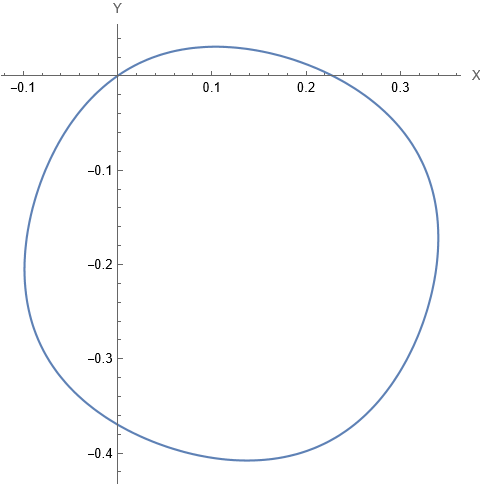
Figure 3: Trajectory of massless Skyrmion under circularly polarized light

4.2.6 Skyrmion’s Trajectory: Massive case

Fluctuations in the spin lattice, such as phonons or other wave-like excitations, could induce inertia on the Skyrmion. Let us introduce the Skyrmion mass, $M_{S}$ into our equation of motion, such that (16) becomes

$$M_{S}\ddot{X}+\mathcal{G}_{xx}\dot{X}+\mathcal{G}_{xy}\dot{Y}+4\pi\left(Q\dot{Y}+J_{Q,y}\right) = D_{x}\penalty 10000\ ,$$ (74)

$$M_{S}\ddot{Y}+\mathcal{G}_{xy}\dot{X}+\mathcal{G}_{yy}\dot{Y}-4\pi\left(Q\dot{X}+J_{Q,x}\right) = D_{y}\penalty 10000\ .$$ (75)

These equations can be solved directly in a similar manner with the previous massless Skyrmion case. The system of equations above can be recast as

$$\frac{d\textbf{V}}{dt}+P(t)\cdot\textbf{V}=\textbf{p}(t),$$ (76)

where $p$ and q is given by

$$P=\frac{1}{M_{S}}\begin{bmatrix}\mathcal{G}_{xx}&\mathcal{G}_{xy}+4\pi Q\\ \mathcal{G}_{xy}-4\pi Q&\mathcal{G}_{yy}\end{bmatrix},\penalty 10000\ \textbf{p}=\frac{1}{M_{S}}\begin{bmatrix}D_{x}-4\pi J_{Q,y}\\ D_{y}+4\pi J_{Q,x}\end{bmatrix}.$$ (77)

Since $P$ is diagonalizable, the vector equation above is equivalent with two general first order ODE which asymptotically converges to the driving term, p. This is due to the fact that in the solution, the homogeneous part which depends on the initial condition, is suppressed by a factor of $\left(\exp\left(\int P(t)dt\right)\right)^{-1}$ at large $t$. This results in a large-time behaviour that does not depend on the initial condition, known as the limit cycle.

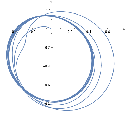
Figure 4: Trajectory of massive Skyrmion under circularly polarized light

To study the behaviour of the limit cycle under variations of the physical parameters, we define the average velocity of the Skyrmion as $v\equiv\sqrt{\langle\dot{X}^{2}+\dot{Y}^{2}\rangle_{t}}$ and the stationary displacement as $\tilde{\textbf{d}}=(\tilde{d}_{x},\tilde{d}_{y})\equiv\left(\langle X\rangle_{t}-X(0),\langle Y\rangle_{t}-Y(0)\right)$, where $\langle\cdot\rangle_{t}$ denotes the time-averaged quantity inside the bracket. $v$ has a geometrical interpretation, namely the effective radius of the limit cycle in momentum space, such that the area of the orbit of $\dot{\textbf{R}}$ is $\pi v^{2}$. Both of these quantities proportionally increase as $B_{0}$ is increased, which implies that the Skyrmion is displaced further from its initial point for stronger light intensity. However, the confinement area of the Skyrmion at large $t$ also becomes larger for stronger intensity since it is proportional to $v$. The phenomenological $M_{S}$ is linearly proportional to the relaxation approaching the limit cycle, but does not affect the displacement of the Skyrmion. Instead, the displacement depends on the $\varphi_{0}$ which cannot be controlled by external perturbation.

In Fig. 5 we show the dependence of the components of $\tilde{\textbf{d}}$ against $\varphi_{0}$. This leads to different types of Skyrmions having different trajectories. Although the magnitude of the displacement is not sensitive to the change in $\varphi_{0}$, its direction does depend on $\varphi_{0}$. Resulting in a continuous family of confinement regions that is parameterized by $\varphi_{0}$. For a group of Skyrmions containing randomly distributed $\varphi_{0}$, this family of confinements resembles a ring-like region around their initial position.

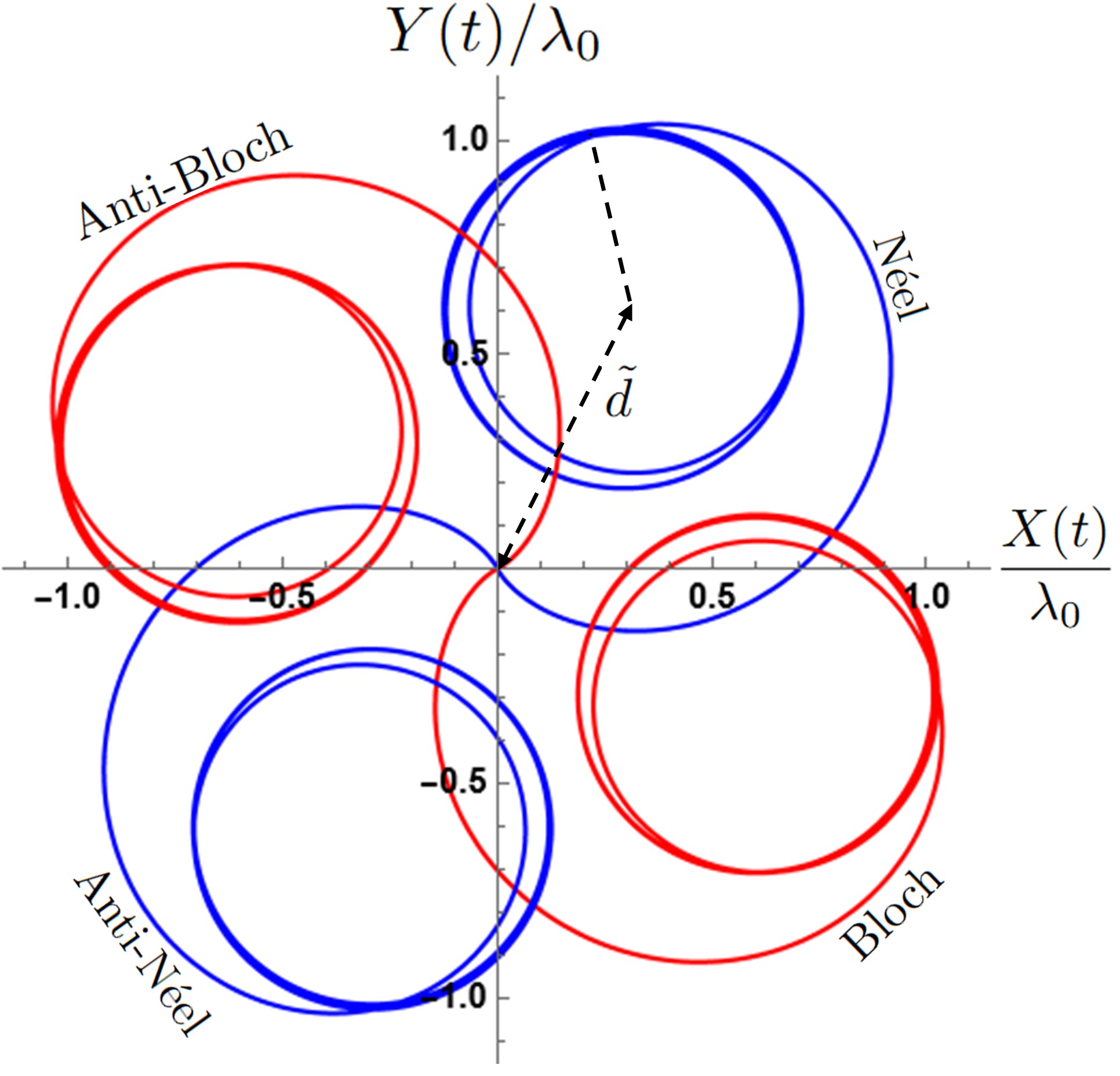
Figure 5: (blue curve) Trajectory of Neel ($\varphi_{0}=0$) and anti-Neel ($\varphi_{0}=\pi$) Skyrmion, and (red curve) Trajectory of Bloch ($\varphi_{0}=\pi/2$) and anti-Bloch ($\varphi_{0}=-\pi/2$) Skyrmion. We use $\eta_{1}/\eta_{2}=\alpha\gamma=1$ and $M_{S}\omega=40$ for the numerical calculation. The displacement magnitude is effectively the distance to the center of the confined orbit R in real-space.

5 Conclusions and Outlooks

Our findings demonstrate that the trajectory of a magnetic Skyrmion governed by an explicitly time-dependent Hamiltonian can be manipulated through its Skyrmion number current. We show that this current can be induced by an oscillating magnetic field—specifically, we illustrate the effect using circularly polarized light of constant intensity. By adjusting $B_{0}$, and hence the ratio $\eta_{1}/\eta_{2}$, the Skyrmion’s trajectory can be finely tuned.

Within this framework, we propose that the optical control of magnetic Skyrmions—recently achieved in micromagnetic simulations [6, 8] and experimentally realized in magnetic multilayers [23]—is fundamentally driven by Skyrmion number current dynamics. This suggests a direct link between the topological nature of Skyrmions and experimentally measurable properties, extending beyond mere conservation of the Skyrmion number. The hypothesis can be tested by examining the motion of a Skyrmionium ($Q=0$) under the same circularly polarized light and comparing its behavior to that of a $Q=1$ Skyrmion. Since the model predicts zero current in the non-topological sector, the Skyrmionium should exhibit a smaller average velocity. A similar comparison could be carried out with Skyrmion bags ($Q>1$), provided the magnetic field is weak enough to avoid significant higher-order perturbations.

Consistent with earlier work by Fujita and Sato [4, 5], who investigated orbital angular momentum (OAM) transfer to magnetic systems, we use light carrying spin angular momentum (SAM) but no OAM, and observe a similar influence on the Skyrmion profile. We therefore suggest that the driving mechanism for Skyrmion motion is the transfer of angular momentum in its most general sense, encompassing both SAM and OAM. This viewpoint naturally accounts for the different trajectories exhibited by Skyrmions of varying helicities. However, to rigorously test this idea, more realistic models must be considered, as specific interaction symmetries could suppress angular momentum transfer. Such is a challenge that we identify as an important direction for future research.

Acknowledgements – E. S. F. acknowledges the support from Badan Riset dan Inovasi Nasional through the Post-Doctoral Program 2024.

References

• [1] A. Bogdanov and A. Hubert. Thermodynamically stable magnetic vortex states in magnetic crystals. Journal of Magnetism and Magnetic Materials, 138(3):255–269, 1994.
• [2] A. N. Bogdanov and D. A. Yablonskii. Thermodynamically stable “vortices” in magnetically ordered crystals. The mixed state of magnets. Soviet Journal of Experimental and Theoretical Physics, 68(1):101, Jan. 1989.
• [3] A. Casiraghi, H. Corte-León, M. Vafaee, F. Garcia-Sanchez, G. Durin, M. Pasquale, G. Jakob, M. Kläui, and O. Kazakova. Individual skyrmion manipulation by local magnetic field gradients. Communications Physics, 2(1):145, 2019.
• [4] H. Fujita and M. Sato. Encoding orbital angular momentum of light in magnets. Physical Review B, 96(6):060407, 2017.
• [5] H. Fujita and M. Sato. Ultrafast generation of skyrmionic defects with vortex beams: Printing laser profiles on magnets. Physical Review B, 95(5):054421, 2017.
• [6] S. Guan, Y. Liu, Z. Hou, D. Chen, Z. Fan, M. Zeng, X. Lu, X. Gao, M. Qin, and J.-M. Liu. Optically controlled ultrafast dynamics of skyrmion in antiferromagnets. Physical Review B, 107(21):214429, 2023.
• [7] S.-G. Je, H.-S. Han, S. K. Kim, S. A. Montoya, W. Chao, I.-S. Hong, E. E. Fullerton, K.-S. Lee, K.-J. Lee, M.-Y. Im, et al. Direct demonstration of topological stability of magnetic skyrmions via topology manipulation. ACS nano, 14(3):3251–3258, 2020.
• [8] M. Kazemi, A. Kudlis, P. F. Bessarab, and I. Shelykh. All-optical control of skyrmion configuration in cri 3 monolayer. Scientific Reports, 14(1):11677, 2024.
• [9] S. Komineas and N. Papanicolaou. Skyrmion dynamics in chiral ferromagnets. Physical Review B, 92(6):064412, 2015.
• [10] M. Lee, W. Kang, Y. Onose, Y. Tokura, and N. P. Ong. Unusual hall effect anomaly in mnsi under pressure. Physical review letters, 102(18):186601, 2009.
• [11] S. Luo, M. Song, X. Li, Y. Zhang, J. Hong, X. Yang, X. Zou, N. Xu, and L. You. Reconfigurable skyrmion logic gates. Nano letters, 18(2):1180–1184, 2018.
• [12] N. S. Manton and P. Sutcliffe. Topological solitons. Cambridge University Press, 2007.
• [13] A. Neubauer, C. Pfleiderer, B. Binz, A. Rosch, R. Ritz, P. Niklowitz, and P. Böni. Topological hall effect in the a phase of mnsi. Physical review letters, 102(18):186602, 2009.
• [14] N. Papanicolaou and T. Tomaras. Dynamics of magnetic vortices. Nuclear Physics B, 360(2-3):425–462, 1991.
• [15] B. M. A. G. Piette, B. J. Schroers, and W. J. Zakrzewski. Dynamics of baby skyrmions. Nucl. Phys. B, 439:205–235, 1995.
• [16] B. M. A. G. Piette, B. J. Schroers, and W. J. Zakrzewski. Multi - solitons in a two-dimensional Skyrme model. Z. Phys. C, 65:165–174, 1995.
• [17] A. M. Polyakov and A. A. Belavin. Metastable States of Two-Dimensional Isotropic Ferromagnets. JETP Lett., 22:245–248, 1975.
• [18] T. Schulz, R. Ritz, A. Bauer, M. Halder, M. Wagner, C. Franz, C. Pfleiderer, K. Everschor, M. Garst, and A. Rosch. Emergent electrodynamics of skyrmions in a chiral magnet. Nature Physics, 8(4):301–304, 2012.
• [19] T. Skyrme. A Nonlinear field theory. Proc. Roy. Soc. Lond. A, A260:127–138, 1961.
• [20] T. H. R. Skyrme. A Unified Field Theory of Mesons and Baryons. Nucl, Phys., 31:556–569, 1962.
• [21] M. Stone. Magnus force on skyrmions in ferromagnets and quantum hall systems. Physical Review B, 53(24):16573, 1996.
• [22] G. Tatara, H. Kohno, and J. Shibata. Microscopic approach to current-driven domain wall dynamics. Physics Reports, 468(6):213–301, 2008.
• [23] T. Titze, S. Koraltan, T. Schmidt, D. Suess, M. Albrecht, S. Mathias, and D. Steil. All-optical control of bubble and skyrmion breathing. Physical review letters, 133(15):156701, 2024.
• [24] M. Xu, Y. Chen, W. Chen, C. Hu, Z. Zhang, G. Jiang, and J. Zhang. Reconfigurable skyrmion logic gates with auto-annihilating skyrmion function. Physica Scripta, 98(10):105939, 2023.
• [25] J. Zang, M. Mostovoy, J. H. Han, and N. Nagaosa. Dynamics of skyrmion crystals in metallic thin films. Physical review letters, 107(13):136804, 2011.
• [26] X. Zhang, Y. Zhou, K. M. Song, T.-E. Park, J. Xia, M. Ezawa, X. Liu, W. Zhao, G. Zhao, and S. Woo. Skyrmion-electronics: writing, deleting, reading and processing magnetic skyrmions toward spintronic applications. Journal of Physics: Condensed Matter, 32(14):143001, 2020.