A Semi-supervised Generative Model for Incomplete Multi-view Data Integration with Missing Labels

Abstract

Multi-view learning is widely applied to real-life datasets, such as multiple omics biological data, but it often suffers from both missing views and missing labels. Prior probabilistic approaches addressed the missing view problem by using a product-of-experts scheme to aggregate representations from present views and achieved superior performance over deterministic classifiers, using the information bottleneck (IB) principle. However, the IB framework is inherently fully supervised and cannot leverage unlabeled data. In this work, we propose a semi-supervised generative model that utilizes both labeled and unlabeled samples in a unified framework. Our method maximizes the likelihood of unlabeled samples to learn a latent space shared with the IB on labeled data. We also perform cross-view mutual information maximization in the latent space to enhance the extraction of shared information across views. Compared to existing approaches, our model achieves better predictive and imputation performance on both image and multi-omics data with missing views and limited labeled samples.

Introduction

Many machine learning (ML) tasks involve data from multiple modalities or “views” (used interchangeably). A sample can have multiple views or modalities. For example, a cartoon illustration of a cat and a photo of a cat are of different modalities but constitute the same latent characteristics of a cat and label (a cat, instead of a dog). Similarly, DNA methylation and mRNA expression values can describe the same underlying physiological condition of the subject and predict their outcome, e.g., disease status. Multi-view paradigms have been applied to various domains. A recent trend is to use semantically similar parts of the input or different augmentations of the input as two views to extract universally useful features for downstream tasks in a self-supervised learning setup (Veličković et al. 2019; Chen et al. 2020; Caron et al. 2020; Tian, Krishnan, and Isola 2020; Bardes, Ponce, and LeCun 2022), and to extract such features from more than two views, e.g., multiple augmentations used for representation learning (Tian, Krishnan, and Isola 2020; Tong et al. 2024); text, video, and audio jointly presented in affective computing (Zadeh et al. 2016; Bagher Zadeh et al. 2018; Castro et al. 2019; Hasan et al. 2019); video, audio, and optical flow jointly presented in human action video data (Kay et al. 2017); image, force sensor, and proprioception sensor jointly presented in robotic applications (Lee et al. 2019, 2020).

For the majority of existing multi-view benchmark datasets, aligned data collection ensures maximal information overlap across views (Ngiam et al. 2011; Wu and Goodman 2018; Zhang et al. 2019; Tsai et al. 2019; Pham et al. 2019; Ma et al. 2021; Huang et al. 2020; Lee and Pavlovic 2021; Lee and van der Schaar 2021). In this work, we are interested in real-world multi-view data where some observations (samples) whose views and label are partially missing. Multi-omics data is a crucial application area of the multi-view learning paradigm with these traits. They are multi-modal by nature and can be used to understand the underlying molecular disease mechanisms and to predict patient outcome e.g., mortality and cancer types (Subramanian et al. 2020). Furthermore, due to limited experimental resources, clinical designs, and sequencing platform differences, these types of data often contain arbitrary missing views and/or missing labels, and discarding such samples reduces sample sizes and can make downstream analysis less reliable (Rappoport and Shamir 2019; Zhao et al. 2023). Therefore, our goal is to develop a unified framework, where maximal amount of information in the dataset can be leveraged for both prediction and imputation.

Our Contributions

(1) We propose a semi-supervised setup for integrated multi-view prediction and missing-view imputation instead of a fully supervised setup, which is only capable of prediction. (2) We introduce a cross-view mutual information loss to this setup, which maximizes the predictive information among different view pairs, to learn a robust joint latent representation. (3) We show the potential of this unified framework to be deployed in biomedical research for better outcome prediction and missing value imputation.

Our Method

Problem Setup

Notations

Our dataset consists of a total of $V$ input views. Let $x_{v}$ be the $d_{v}$ dimensional input feature from the $v$-th view and $y\in\mathcal{Y}$ be the output label. $x_{v}=\varnothing$ if the $v$-th view is missing, and $y=\varnothing$ if the label is missing and available if $y\in\mathcal{Y}$. A set of observed views can be denoted by $\mathcal{V}=\{v:x_{v}\neq\varnothing\}$, with the input features being $X=\{x_{v}:v\in\mathcal{V}\}$. A data sample $(X,y)$ is incomplete if $x_{v}=\varnothing$ for some view $v$ and/or $y=\varnothing$. We have a dataset $\mathcal{D}=\{X_{n},y_{n}\}_{n=1}^{N}$ where each sample $(X_{n},y_{n})$ may be incomplete. The set of samples with observed labels are referred to as the supervised portion whereas the rest unsupervised.

Problem Statement

Under the multi-view redundancy assumption that different views provide the same predictive information, our goal is to extract a latent representation $z$ from a multi-view observation $X$ with an arbitrary view-missing pattern, for the purpose of predicting target $y$. We focus on the semi-supervised setup where ground truth labels are only present for a small portion of the dataset, so we need to leverage large amount of unlabeled data for learning a discriminative representation. We use variational methods to extract a common subspace shared by the views, based on which we perform both reconstruction of missing inputs and prediction of discrete labels. Our setup can be viewed as a generalization of DeepIMV (Lee and van der Schaar 2021) by allowing missing labels.

The incomplete multi-view problem involves two major challenges. First, the learned representations must integrate incomplete observations with various view-missing and label-missing patterns in a unified framework. Second, the learned representation must integrate information shared across views that are relevant to the prediction task.

Loss Components

To address these challenges, we propose a semi-supervised representation learning framework that consists of the following loss components. The overall architecture is shown in Figure 2.

PoE-based Joint View Representation

One can first realize a common latent space by probabilistically encoding each view with the posterior distribution $q_{\theta}(z_{v}|x_{v})$ (Kingma and Welling 2019) and aggregate all encoded present views into a joint representation $q_{\theta}(z|X)$, where $\theta$ represents encoding parameters. This joint representation is used for both supervised cross-entropy loss ($\mathcal{L}_{\text{sup}}$, on labeled data) and unsupervised loss ($\mathcal{L}_{\text{unsup}}$, on unlabeled data). To aggregate individual representations of each view (which may be absent) generated by view-specific variational autoencoders (VAEs) into a joint representation, one may use PoE, which is defined as follows (Wu and Goodman 2018):

$$q_{\theta}(z|X)\propto p(z)\prod_{v\in\mathcal{V}}q_{\theta}(z|x_{v}).$$ (1)

The prior $p(z)$ is a simple Gaussian with zero mean and unit variance. And when $q_{\theta}(z|x_{v})$ are parameterized as Gaussians, $q_{\theta}(z|X)$ is also Gaussian, whose mean and variance can be computed in closed-form form local posteriors of the present views.

Supervised Information Bottleneck (IB) on Labeled Data

On supervised data $(X,y)$, we estimate the predicted label $y$ based on $q_{\psi}(y|z)$, given the latent sample $z$ drawn from $q_{\theta}(z|X)$, where $\psi$ represents predictor parameters.

To ensure the robustness and generalization of the prediction model of $X\rightarrow z\rightarrow y$, the IB principle maximizes the task-relevant information in $z$, i.e., $I(y;z)$, to correctly predict the label $y$, and minimize redundant, or irrelevant, information $I(X,z)$ to reduce the effect of nuisance factors in data. One can derive the following variational objective based on the IB principle (Lee and van der Schaar 2021):

$$\mathcal{L}_{\text{sup}}^{\theta,\psi}(X,y) =-I(y;z)+\beta I(X;z)$$ (2)

$$\approx\mathbb{E}_{X,y}\mathbb{E}_{z\sim q_{\theta}(z|X)}\bigl[-\log q_{\psi}(y|z)\bigr]$$

$$+\beta\mathbb{E}_{X}\bigl[\textrm{KL}(q_{\theta}(z|X)\|q(z)\bigr]$$

where the first term is the cross-entropy loss between prediction and ground truth $y$ and the second term is the Kullback-Leibler (KL) divergence between the joint posterior and prior, which prevents posterior from deviating significantly from the prior $q(z)$, a simple distribution independent from the data (e.g., the standard Gaussian). Here $\beta>0$ is a user-defined hyperparameter that is set to 0.1 throughout this paper. We also attach a KL term for each view separately, i.e., $\beta\sum_{v\in\mathcal{V}}\mathbb{E}_{x_{v}\sim p(x_{v})}\bigl[\textrm{KL}(q_{\theta}(z_{v}|x_{v})\|q(z_{v})\bigr]$ as we find it to improve numerical stability.

Generative modeling on Unabeled Data

When we only have a small amount of labels, the IB loss may fail to extract a robust representation. Therefore, we propose to improve representation learning using unlabeled data with missing views. Our intuition is to enforce $z$ to model important variations of the data so that it generates/reconstructs the observed data well. This is naturally done with a multimodal VAE objective as follows (Wu and Goodman 2018):

$$\mathcal{L}_{\text{unsup}}^{\theta,\phi}(X) =-\mathbb{E}_{X}\Bigl[\mathbb{E}_{z\sim q_{\theta}(z|X)}\Bigl[\sum_{v\in\mathcal{V}}\log p_{\phi}(X_{v}|z)\Bigr]$$ (3)

$$-\beta\textrm{KL}\bigl[q_{\theta}(z|X)\|p(z)\bigr]\Bigr]$$

where $\phi$ refers to the parameters in the decoders which provide $\log p_{\phi}(X_{v}|z)$. The negative of (3) is the evidence lower bound (ELBO) of the observed input data. This generative approach facilitates missing view imputation: we can obtain the joint posterior $q_{\phi}(z|X)$ from the observed views, and provide the sample of this distribution to the decoder of the missing view for generation.

Cross-view Mutual Information Regularization

We observe that in Equation (3), likelihood maximization encourages $z$ to contain high mutual information about $X$. This is because $I(z;X)=H(X)-H(X|z)$ where the entropy $H(X)$ is a constant, and minimizing the conditional entropy

$$H(X|z) =-\int p(X,z)\log p(X|z)dzdX$$

$$=\mathbb{E}_{X,z}[-\log p(X|z)]$$

is equivalent to maximizing conditional likelihood. However, this approach requires a good likelihood model $p(X|z)$ which may be challenging for high dimensional structured data (e.g., for images, the dimensionality of inputs is the number of pixels). Alternatively, based on the multi-view redundancy assumption that that two views provide the same predictive information, we can focus on extracting the shared information in the latent space directly using unlabeled data.

To see this, recall that the mutual information term between the view and its representation can be factorized using the chain rule:

$$I(x_{1};z_{1})=I(x_{1};z_{1}|y)+I(z_{1};y).$$ (4)

Here $z_{1}$ is the representation of $x_{1}$, modeled by the posterior $q(z_{1}|x_{1})$. In this decomposition, $I(x_{1};z_{1}|y)$ represents the superfluous information (the information in $x_{1}$ that is not predictive of $y$), and $I(z_{1};y)$ represents the predictive information. When $y$ is observed, we can maximize $I(z_{1},y)$ and minimize $I(x_{1};z_{1}|y)$ as in supervised IB.

When the label $y$ is not observed, one can guarantee that $z_{1}$ is sufficient for predicting $y$ without knowing $y$, i.e., circumvent supervision, if the multi-view redundancy assumption holds. The assumption requires that the two views are mutually redundant, i.e., $I(y;x_{1}|x_{2})=I(y;x_{2}|x_{1})=0$. A schematic diagram of the assumption is given in Figure 1, where the variation of $y$ that is predictable from $x_{1}$ and $x_{2}$ is contained entirely in their intersection. As a result of this assumption, any representation containing all the information shared by both views is as predictive as their joint observation (Federici et al. 2020) [Corrollary 1].

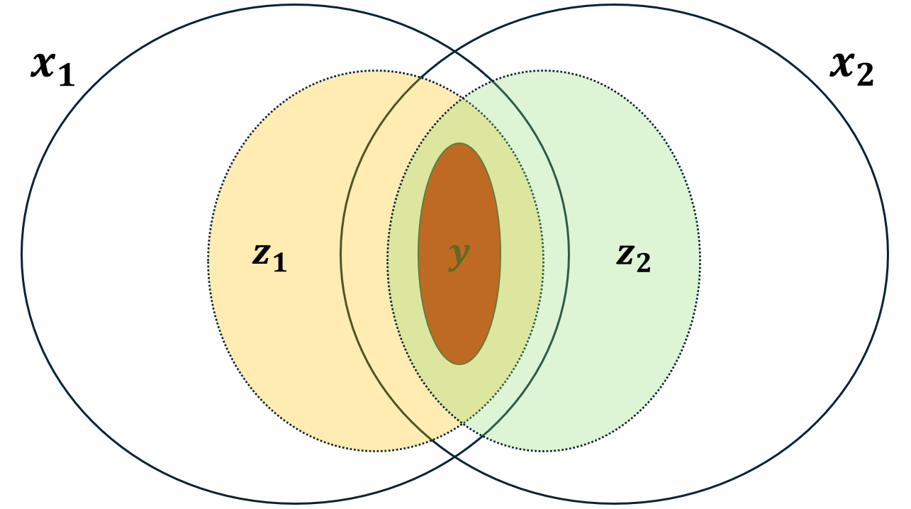
Figure 1: Multi-view redundancy assumption and mutual information decomposition. Since $y$ lies in the intersection of $x_{1}$ and $x_{2}$, we encourage $z_{1}$ to capture information about $x_{2}$ so as to capture information about $y$.

This result motivates us to use $x_{2}$ as a proxy of $y$ and enforce $z_{1}$ to contain high mutual information with $x_{2}$, which can be further lower bounded as:

$$I(z_{1},x_{2}) =I(z_{1};z_{2}x_{2})-I(z_{1};z_{2}|x_{2})$$ (5)

$$=I(z_{1};z_{2}x_{2})$$

$$=I(z_{1};z_{2})+I(z_{1};x_{2}|z_{2})$$

$$\geq I(z_{1};z_{2})$$

where $z_{2}$ is the representation of $x_{2}$ as modeled by $q(z_{2}|x_{2})$ (and therefore $I(z_{1};z_{2}|x_{2})=0$ in the first step due to its variability coming from $x_{2}$ and not $x_{1}$).

In this work, we use the contrastive estimate of mutual information (Oord, Li, and Vinyals 2018) as regularization:

$$I(z_{1};z_{2})\approx\mathbb{E}_{z_{1},z_{2}}\log\left[\frac{\phi(z_{1},z_{2})}{\phi(z_{1},z_{2})+\sum_{j=1}^{n}\phi(z_{1},\bar{z}_{2}^{j})}\right]$$ (6)

where $\phi(z_{1},z_{2})=\exp\left(\frac{z_{1}^{\top}z_{2}}{\lVert z_{1}\rVert\cdot\lVert z_{2}\rVert}\right)$ is the affinity function, and $\bar{z}_{2}^{j}$ are $n$ negative examples randomly sampled from the minibatch not aligned with $z_{1}$. In (6), the expectation is computed over samples for which both view 1 and 2 are observed. In practice, we use the symmetrized version of (6) in which we switch the role of the two views and average the two estimates. Intuitively, this loss enforces the latent representation for paired data $(x_{1},x_{2})$ to be similar while representations of unpaired data are pushed far apart.

Note that when our dataset consists of more than two views, we maximize the average of the above estimate computed for all pairs of views (Tian, Krishnan, and Isola 2020), or equivalently minimize

$$\mathcal{L}_{\text{cvmi}}(z)=-\frac{1}{\binom{V}{2}}\sum_{i\neq j}I(z_{i};z_{j})$$ (7)

We comment that for many multi-view learning problems, the redundancy assumption is approximately satisfied as evidenced by our experimental results, where $\mathcal{L}_{\text{cvmi}}(z)$ can significantly boost the performance when likelihood modeling is challenging.

Overall Objective

Our final objective combines the above intuitions:

$$\min\mathcal{L}_{\text{total}}^{\phi,\psi,\theta}(X,y)=\mathcal{L}_{\text{unsup}}^{\theta,\phi}(X)+\gamma\mathcal{L}_{\text{sup}}^{\theta,\psi}(X,y)+\alpha\mathcal{L}_{\text{cvmi}}(z)$$ (8)

where $\gamma$ and $\alpha$ are hyperparameters to be tuned on validation data. An illustration of our model is given in Figure 2.

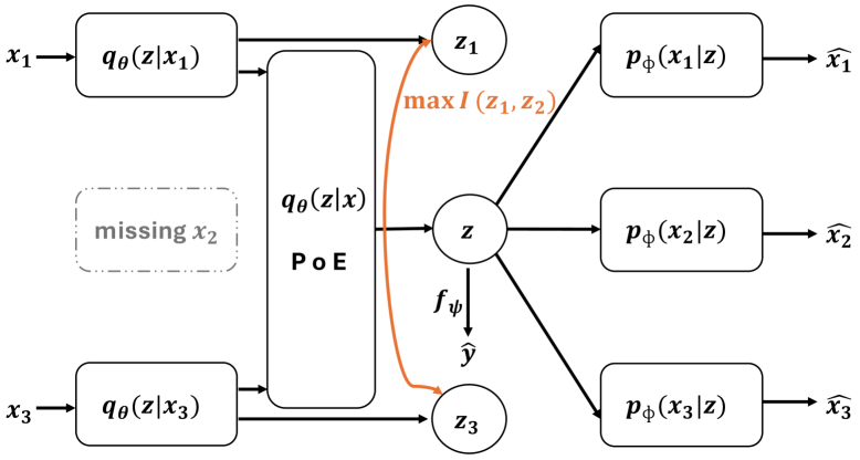
Figure 2: The architecture of our method.

Related Works

Multi-view observations are prevalent in real-world datasets. To utilize information across data with more than one modalities, canonical correlation analysis (CCA) and their extensions were proposed to utilize the the latent space between two views where the canonical correlation is maximized (Hotelling 1936; Andrew et al. 2013). However, these methods cannot utilize data with missing views and require imputation, which may distort data quality. Multi-view/Multi-modal generative models (Wang et al. 2016; Suzuki, Nakayama, and Matsuo 2016) have the potential to deal with missing views. Recent works have extended this approach to more than two modalities and missing-view data and have shown promising results. For example, MMVAE (Shi et al. 2019) uses a mixture of experts aggregation scheme to learn generative models on different sets of modalities; MVAE (Wu and Goodman 2018) uses a PoE inference network to learn the latent space under different combinations of missing views; and MoPoE-VAE (Sutter, Daunhawer, and Vogt 2021), which uses mixture-of-product-of-experts, claimed to combine the good of both worlds by approximating the joint posterior for all subsets of modalities. While promising, they are inherently unsupervised learning methods and require multi-stage training for prediction tasks, that is, learning a latent representation before training a predictor. CPM-Nets (Zhang et al. 2019) assumes a common latent space for both inputs and targets similarly to us, and it treats the latent representations of training data as free variables for optimizing the combination of reconstruction and prediction losses, but they suffer from the out-of-sample problem for test data and is therefore less convenient to use.

Another set of deep generative models were motivated by the information bottleneck method (Tishby, Pereira, and Bialek 1999; Tishby and Zaslavsky 2015; Achille and Soatto 2018). In (Alemi et al. 2017), the authors proposed a variational information bottleneck (VIB) method to extract $Z$ from $X_{1}$ which has high MI with $X_{2}$, so that it captures the shared information, and at the same time has low MI with $X_{1}$ so that it contains little nuisance factors. Starting from a different generative assumption, the VIB learning objective turned out to be similar to the VCCA objective of (Wang et al. 2016), with the main difference of VIB not including an auto-encoding loss, i.e., their method only had the cross-view generation path $X_{1}\rightarrow Z_{1}\rightarrow X_{2}$, but not the self-reconstruction path $X_{1}\rightarrow Z_{1}\rightarrow X_{1}$. In (Federici et al. 2020), the authors introduced the multi-view redundancy assumption that all the information $X_{1}$ contains about an unobserved label $y$ is also contained in $X_{2}$. Under this assumption, the authors showed that if the learned representation $Z_{1}$ is sufficient in the sense that $I(X_{1},X_{2}|Z_{1})=0$, then $Z_{1}$ will have all the predictive power from $(X_{1},X_{2})$ for $y$. Remarkably, their multi-view information bottleneck (MVIB) objective did not involve any reconstruction paths, and the authors considered this to be an advantage, given that density modeling for high dimensional data is difficult. We note that these works mostly work with two view data without missing views.

Mutual information-based method has received significant attention in the past a few years, due to its applications to self-supervised learning. Self-supervised learning is a paradigm that aims at learning useful representations from large amounts of unlabeled data, by creating artificial targets that are generally correlated with downstream tasks, so that the downstream supervised learning on top of these learned representations requires a minimal amount of labels. Self-supervised learning can be applied to a single modality, with artificial views created based on the structures of data. For example,  (Oord, Li, and Vinyals 2018) used the high-level representations of an audio segment and its nearby segments as the views, and an image patch and its nearby patches as the views  (Hjelm et al. 2019; Bachman, Hjelm, and Buchwalter 2019) used global features and local features of images as the views;  (Chen et al. 2020) used the two augmented versions of the same image. Many of these methods were motivated by the classical infomax principle (Linsker 1988). While our cross-view MI loss shares similar intuitions with them, the focus of our work is semi-supervised multi-view learning with missing data.

Experiments

Baselines

We compare our method against three methods.

• Supervised baseline (Base): uses generic encoders (MLP or ResNet) followed by a linear layer for each view. The classifiers are trained with the cross-entropy loss using paired (input, label) that are present. At inference time, we average logits of present views for making predictions.

• MVAE (Wu and Goodman 2018): based on the product-of-expert (PoE) aggregation scheme, it extracts a global latent representation across multiple views to maximize ELBO of observed input data. After unsupervised representation learning is done, a deterministic MLP is trained using paired (global latent representation, label) similarly to Base.

• DeepIMV (Lee and van der Schaar 2021): uses the PoE scheme to aggregate latent posteriors of present views, to directly predict labels. The model is trained with the IB objective using paired (input, label) that are present.

To evaluate these different methods, we measured the area under the receiver operating characteristic (AUROC) and accuracy values on the validation/test sets. For both metrics, the range is $[0,1]$ where a higher value indicated better performance.

The Cancer Genome Atlas (TCGA) Dataset

Experimental Setup

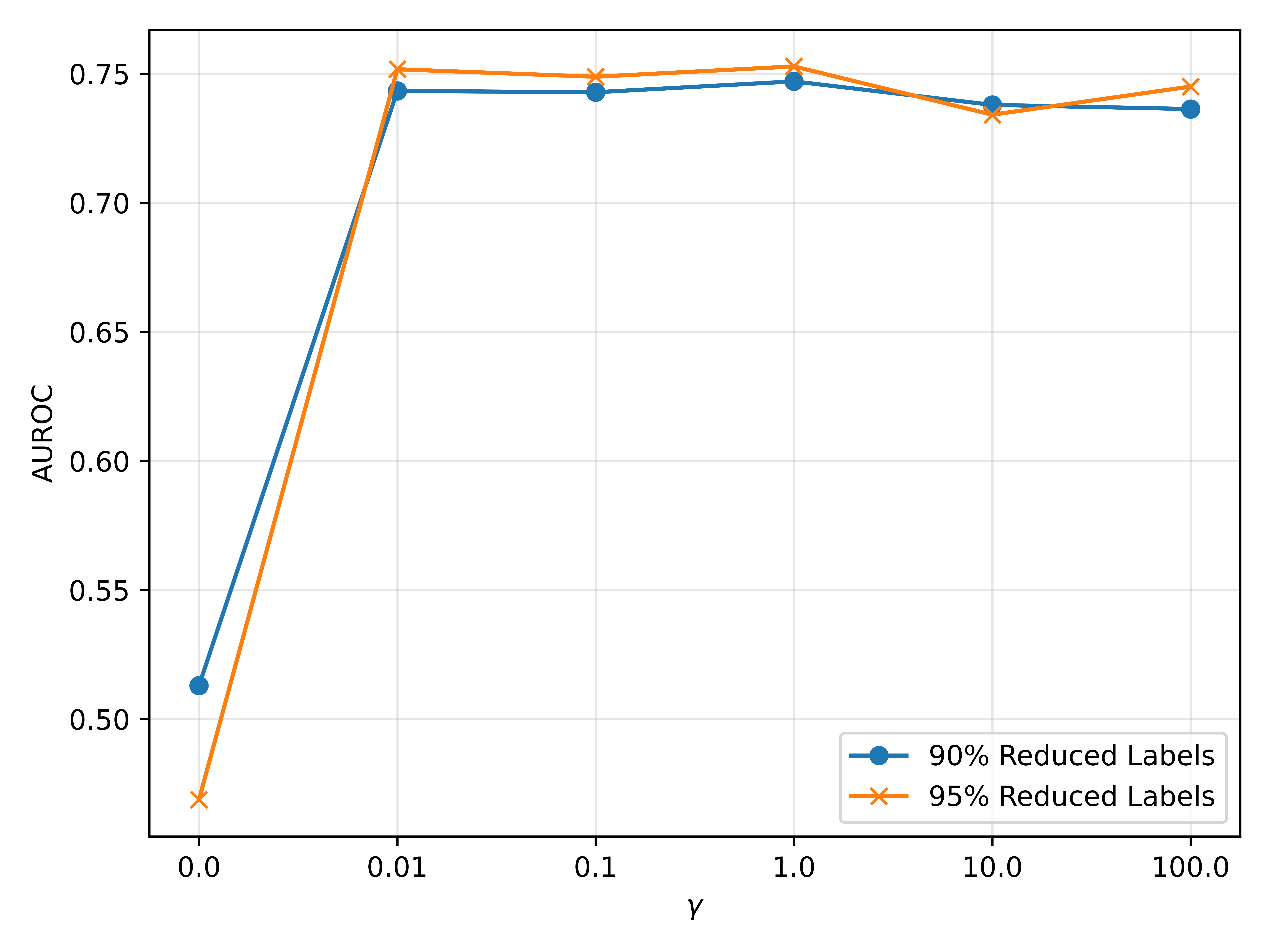
Figure 3: The AUROC performance for TCGA validation dataset regarding different values of $\gamma$ while setting $\alpha$ to be 10.0.

Figure 4: The AUROC performance for TCGA validation dataset regarding different values of $\alpha$ while setting $\gamma$ to be 0.1.

Our first set of experiments were done on a real-world multi-omics dataset collected from the Cancer Genome Atlas (TCGA) with 10,960 patient samples, of which 9,477 are non-censored/labeled patient samples. Each sample has four views: mRNA expressions, DNA methylation, microRNA (miRNA) expressions, and reverse phase protein assay (RPPA). We applied the data-preprocessing procedure of Lee and van der Schaar 2021 to obtain input features, which essentially selects features that are shared among all patients and perform a kernel PCA to transform each raw sample into a 100-dimensional continuous representation. The label was converted from days of survival upon cancer diagnosis to binary 1-year mortality. We further performed z-score standardization on these representations and the resulting features are used as inputs to all methods.

Non-censored (labeled) patient samples underwent 64/16/20 train/validation/test splits before the training set labels were reduced further by 90% or 95% to simulate scenarios with severe missing labels. Then all 1,483 originally censored (unlabeled) samples were added to the unsupervised portion of training set so they could be further-utilized to learn a more robust representation of the feature space. The datasets shared mutual information between different views as per Lee and van der Schaar 2021, and is therefore a good testbed for our method. Each view was encoded and decoded with a different 2-layer VAE.

Table 1: Average Prediction on TCGA dataset over 5 Runs with 90% Reduced Training Labels Using Different Methods (left) and Using Base Method on Imputed Views (right).

Method	AUROC	Accuracy
Base	0.7138 $\pm$ 0.0082	0.6851 $\pm$ 0.0048
MVAE	0.5202 $\pm$ 0.0382	0.6394 $\pm$ 0.0048
DeepIMV	0.7234 $\pm$ 0.0016	0.6889 $\pm$ 0.0055
Ours $-\mathcal{L}_{\text{cvmi}}$	0.7377 $\pm$ 0.0055	0.7015 $\pm$ 0.0094
Ours	0.7419 $\pm$ 0.0105	0.6936 $\pm$ 0.0054

Imputation	AUROC	Accuracy
Mean	0.7291	0.6895
MVAE	0.7393	0.6868
Ours	0.7345	0.6943

Table 2: Average Prediction on TCGA dataset over 5 Runs with 95% Reduced Training Labels Using Different Methods (left) and Using Base Method on Imputed Views (right).

Method	AUROC	Accuracy
Base	0.6993 $\pm$ 0.0028	0.6834 $\pm$ 0.0061
MVAE	0.5354 $\pm$ 0.0315	0.6330 $\pm$ 0.0154
DeepIMV	0.7150 $\pm$ 0.0022	0.6869 $\pm$ 0.0071
Ours $-\mathcal{L}_{\text{cvmi}}$	0.7424 $\pm$ 0.0069	0.7049 $\pm$ 0.0115
Ours	0.7523 $\pm$ 0.0078	0.6993 $\pm$ 0.0070

Imputation	AUROC	Accuracy
Mean	0.7160	0.6937
MVAE	0.7232	0.7000
Ours	0.7212	0.7020

Sensitivity Analysis

Ablation studies of the MI term (coefficient $\alpha$, Figure 4) and the CE term (coefficient $\gamma$, Figure 3) were performed on the TCGA validation dataset to show that both terms are beneficial and complementary to each other. When $\alpha$ and $\gamma$ were set to 0 (corresponding to the MVAE method), the AUROC was at the lowest, but when both coefficients were non-zero, drastic improvements were observed and the optimal performance was obtained with $\alpha=10$ and $\gamma=0.1$ for both missing portions. As shown in Figure 3, the performance increased most drastically when $\gamma$ is set to be non-zero, which was expected because the binary cross-entropy loss computed with ground truth labels is directly related to prediction performance. However, the discriminative loss need not to be dominant ($\gamma$ need not be set to be too large) when the amount of labels is small and we apply cross-view MI loss. As shown in Figure 4, a nonzero $\alpha$ resulted in better performance, which demonstrated that the shared information across the views were highly discriminative and compensated the loss of ground truth labels.

Predictive and Imputation Performance

We provided the test set metrics in Table 1 and 2 (left panels), for the 90% missing label and 95% missing label setups, respectively, in which we could see our method consistently outperformed the baselines. Removing the MI term has caused the model to perform slightly worse because the MI term was used to maximize information between different pairs of views. DeepIMV performance was successfully reproduced from  Lee and van der Schaar 2021, which is better than base and MVAE but worse than ours. It is also worth noting that generative models are robust to label scarcity. As seen in the tables, base and DeepIMV suffer from label scarcity as we reduce the amount available labels from 10% to 5%. However, MVAE and our methods did not suffer as much from the lack of labels.

Similar to (Lee and van der Schaar 2021), missing-view imputation was performed by training the model first, sampling in the latent space (as computed by the PoE scheme), and decoding using the view-specific decoder. To evaluate imputation, imputed train/validation/test datasets with labels were evaluated by the Base method, which could only leverage labeled data. In terms of imputation, our method’s performance was on par with MVAE and better than mean imputation (Table 1, 2, right panels) This showed an improvement over Base with missing data, indicating that the likelihood modeling was successful and generated samples were of good quality. Furthermore, since there were more available labels in the 90% reduced label setting than the 95% reduced label setting, the predictive performance in the latter was worse than that of the former.

Translated-PolyMNIST Dataset

Experimental Setup

The second set of experiments were performed on the Translated-PolyMNIST dataset (Daunhawer et al. 2022) with slight modifications. The dataset generation process is as follows. Training MNIST digits were resized from 28x28 to 14x14. Each of the 5 full background images was cropped at random positions 6 times into 28x28 images, and 1 resized MNIST sample was overlaid at a random position on top of the cropped background images. The MNIST samples across the 5 views have the same identity, i.e., the shared variation was guaranteed to contain discriminative information. We could generate 330,000 training samples, 5,000 validation samples, and 10,000 test samples in this fashion. Each view then had 50% inputs randomly dropped, and we ensured that each sample had at least one present view. The labels correspond to the MNIST digit were present in the image. Additionally, the labels of the training set were reduced by 95% (1,650 available labels per class) and 99.5% (165 available labels per class), respectively, to simulate scenarios with minimally available labels to test the robustness of the model. This dataset was quite challenging as the common signal (the digit) consists of a small amount of pixels as compared to the random backgrounds, and multiple VAE methods were shown to fail to extract the digit identity (Daunhawer et al. 2022). Each view was encoded and decoded with ResNet (He et al. 2015).

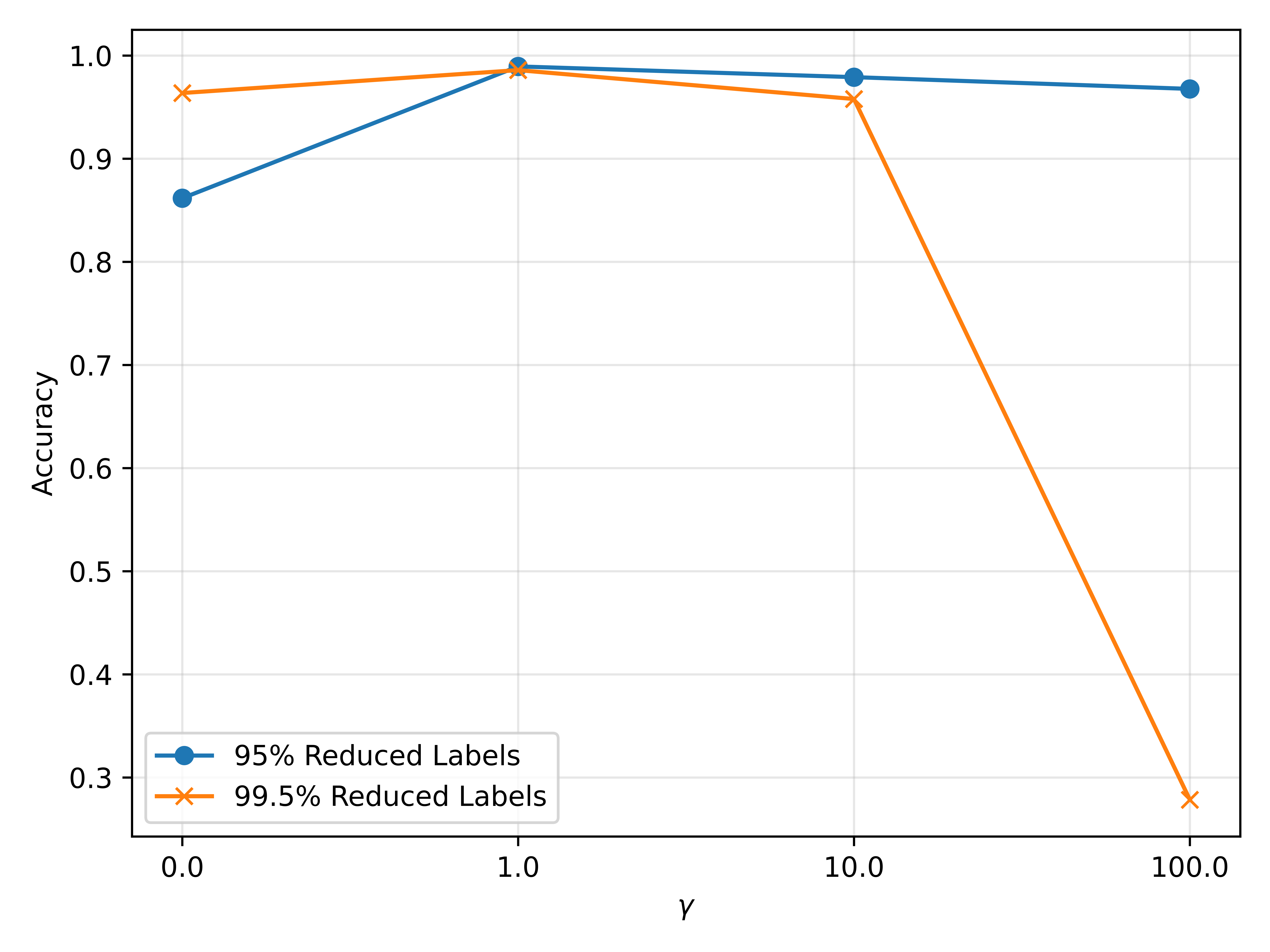
Figure 5: The accuracy for Translated-PolyMNIST validation dataset regarding different values of $\gamma$ while setting $\alpha$ to be 100.0.

Figure 6: The accuracy for Translated-PolyMNIST validation dataset regarding different values of $\alpha$ while setting $\gamma$ to be 1.0.

Sensitivity Analysis

Table 3: Prediction Performance of Translated-PolyMNIST with 95% Reduced Training Labels (left) and 99.5% Reduced Training Labels (Right).

Method	AUROC	Accuracy
Base	0.9709	0.8117
MVAE	0.5981	0.1716
DeepIMV	0.9979	0.9563
Ours $-\mathcal{L}_{\text{cvmi}}$	0.8074	0.3795
Ours	0.9996	0.9886

Method	AUROC	Accuracy
Base	0.5100	0.1097
MVAE	0.5932	0.1719
DeepIMV	0.8802	0.5691
Ours $-\mathcal{L}_{\text{cvmi}}$	0.6287	0.2025
Ours	0.9995	0.9867

Figure 7: Imputation on Translated-PolyMNIST by MVAE (left) and our method (Right). In this dataset, 50% of inputs are missing while 95% labels are missing. Images in red frames are imputed while others are present.

We performed an ablation study on the validation set in a similar fashion as was done with the TCGA dataset. When $\alpha$ and $\gamma$ were set to 0, which corresponds to MVAE, the performance was close to random guessing. Hyperparameter tuning results have shown that $\alpha=100.0$ and $\gamma=1.0$ under both 95% and 99.5% reduced label settings have similarly provided the best validation results, and our methods achieved close to perfect classification. The performance increased modestly when $\gamma$ is set to nonzero (Figure 5). More importantly, setting $\alpha$ to a large value ensures good performance for different missing portions (Figure 6, which shows the validity of our intuition that cross-view MI elicits the common variations.

Predictive and Imputation Performance

Our method has performed consistently better than the baselines (Table 3). In both the reduced label setting 95% and the reduced label setting 99.5%, our method ranked the highest in terms of accuracy. Removing the cross-view MI term caused the model to degrade significantly because the likelihood model was not strong enough to capture the shared information, while the MI term was computed in the latent space and more tractable. It is also worth noting that the performance of generative models were more robust to label scarcity. As seen in the tables, base and DeepIMV suffered from label scarcity as we increased the missing portion. On the other hand, our method’s performance was stable when cross-view MI was used.

We provided samples of imputed images for both MVAE and our method in Figure 7. In general, our method’s performance was superior to that of the MVAE in that the imputation by our method more faithfully represent the digit label information.

Conclusions

In this work, we have introduced a semi-supervised generative model that can utilize unlabeled data with incomplete views for better predictions and imputations, which performs better than existing models on a real-world biological dataset and a difficult synthetic dataset. In experiments, we observed on the Translated-PolyMNIST dataset that while cross-view MI helps extract the shared information, the imputation is not of very high quality. This is likely because other variations of the inputs, which are private to each view, were not captured (e.g., the background of the views are different). In this case, the performance of our method may be improved by incorporating another set of private latent variables in likelihood modeling/generation. We note that private variables were studied in the context of multi-modal generative models (Wang et al. 2016; Lee and Pavlovic 2021; Palumbo, Daunhawer, and Vogt 2023) and we can extend its usage into our missing view setup, which will also allow us to overcome the limitation of the multi-view redundancy assumption (Liang et al. 2023). Another possibility is to apply diffusion models (Sohl-Dickstein et al. 2015; Ho, Jain, and Abbeel 2020; Song et al. 2021) in a multi-view setup (Palumbo et al. 2024).

References

- Achille and Soatto (2018) Achille, A.; and Soatto, S. 2018. Emergence of invariance and disentanglement in deep representations. Journal of Machine Learning Research, 19(1): 1947–1980.
- Alemi et al. (2017) Alemi, A. A.; Fischer, I.; Dillon, J. V.; and Murphy, K. 2017. Deep Variational Information Bottleneck. In ICLR.
- Andrew et al. (2013) Andrew, G.; Arora, R.; Bilmes, J.; and Livescu, K. 2013. Deep Canonical Correlation Analysis. In ICML.
- Bachman, Hjelm, and Buchwalter (2019) Bachman, P.; Hjelm, R. D.; and Buchwalter, W. 2019. Learning representations by maximizing mutual information across views. In NeurIPS.
- Bagher Zadeh et al. (2018) Bagher Zadeh, A.; Liang, P. P.; Poria, S.; Cambria, E.; and Morency, L.-P. 2018. Multimodal Language Analysis in the Wild: CMU-MOSEI Dataset and Interpretable Dynamic Fusion Graph. In Proceedings of the 56th Annual Meeting of the Association for Computational Linguistics.
- Bardes, Ponce, and LeCun (2022) Bardes, A.; Ponce, J.; and LeCun, Y. 2022. VICReg: Variance-Invariance-Covariance Regularization for Self-Supervised Learning. In ICLR.
- Caron et al. (2020) Caron, M.; Misra, I.; Mairal, J.; Goyal, P.; Bojanowski, P.; and Joulin, A. 2020. Unsupervised Learning of Visual Features by Contrasting Cluster Assignments. In NeurIPS.
- Castro et al. (2019) Castro, S.; Hazarika, D.; Pérez-Rosas, V.; Zimmermann, R.; Mihalcea, R.; and Poria, S. 2019. Towards Multimodal Sarcasm Detection (An _Obviously_ Perfect Paper). In Proceedings of the 57th Annual Meeting of the Association for Computational Linguistics.
- Chen et al. (2020) Chen, T.; Kornblith, S.; Norouzi, M.; and Hinton, G. 2020. A Simple Framework for Contrastive Learning of Visual Representations. In ICML.
- Daunhawer et al. (2022) Daunhawer, I.; Sutter, T. M.; Chin-Cheong, K.; Palumbo, E.; and Vogt, J. E. 2022. On the Limitations of Multimodal VAEs. In ICLR.
- Federici et al. (2020) Federici, M.; Dutta, A.; Forré, P.; Kushman, N.; and Akata, Z. 2020. Learning Robust Representations via Multi-View Information Bottleneck. In ICLR.
- Hasan et al. (2019) Hasan, M. K.; Rahman, W.; Bagher Zadeh, A.; Zhong, J.; Tanveer, M. I.; Morency, L.-P.; and Hoque, M. E. 2019. UR-FUNNY: A Multimodal Language Dataset for Understanding Humor. In EMNLP.
- He et al. (2015) He, K.; Zhang, X.; Ren, S.; and Sun, J. 2015. Deep Residual Learning for Image Recognition. arXiv:1512.03385.
- Hjelm et al. (2019) Hjelm, R. D.; Fedorov, A.; Lavoie-Marchildon, S.; Grewal, K.; Bachman, P.; Trischler, A.; and Bengio, Y. 2019. Learning deep representations by mutual information estimation and maximization. In ICLR.
- Ho, Jain, and Abbeel (2020) Ho, J.; Jain, A.; and Abbeel, P. 2020. Denoising diffusion probabilistic models. In NeurIPS.
- Hotelling (1936) Hotelling, H. 1936. Relations between Two Sets of Variates. Biometrika, 28(3/4): 321–377.
- Huang et al. (2020) Huang, Z.; Hu, P.; Zhou, J. T.; Lv, J.; and Peng, X. 2020. Partially View-aligned Clustering. In NeurIPS.
- Kay et al. (2017) Kay, W.; Carreira, J.; Simonyan, K.; Zhang, B.; Hillier, C.; Vijayanarasimhan, S.; Viola, F.; Green, T.; Back, T.; Natsev, P.; Suleyman, M.; and Zisserman, A. 2017. The Kinetics Human Action Video Dataset. ArXiv:1705.06950.
- Kingma and Welling (2019) Kingma, D. P.; and Welling, M. 2019. An Introduction to Variational Autoencoders. Foundations and Trends in Machine Learning.
- Lee and van der Schaar (2021) Lee, C.; and van der Schaar, M. 2021. A Variational Information Bottleneck Approach to Multi-Omics Data Integration. In AISTATS.
- Lee and Pavlovic (2021) Lee, M.; and Pavlovic, V. 2021. Private-Shared Disentangled Multimodal VAE for Learning of Latent Representations. In 2021 IEEE/CVF Conference on Computer Vision and Pattern Recognition Workshops (CVPRW).
- Lee et al. (2020) Lee, M. A.; Yi, B.; Martin-Martin, R.; Savarese, S.; and Bohg, J. 2020. Multimodal Sensor Fusion with Differentiable Filters. In International Conference on Intelligent Robots and Systems (IROS).
- Lee et al. (2019) Lee, M. A.; Zhu, Y.; Srinivasan, K.; Shah, P.; Savarese, S.; Fei-Fei, L.; Garg, A.; and Bohg, J. 2019. Making Sense of Vision and Touch: Self-Supervised Learning of Multimodal Representations for Contact-Rich Tasks. In International Conference on Robotics and Automation (ICRA).
- Liang et al. (2023) Liang, P. P.; Deng, Z.; Ma, M. Q.; Zou, J.; Morency, L.-P.; and Salakhutdinov, R. 2023. Factorized Contrastive Learning: Going Beyond Multi-view Redundancy. In NeurIPS.
- Linsker (1988) Linsker, R. 1988. Self-organization in a perceptual network. Computer, 21(3): 105–117.
- Ma et al. (2021) Ma, M.; Ren, J.; Zhao, L.; Tulyakov, S.; Wu, C.; and Peng, X. 2021. SMIL: Multimodal Learning with Severely Missing Modality. In AAAI.
- Ngiam et al. (2011) Ngiam, J.; Khosla, A.; Kim, M.; Nam, J.; Lee, H.; and Ng, A. 2011. Multimodal Deep Learning. In ICML.
- Oord, Li, and Vinyals (2018) Oord, A. v. d.; Li, Y.; and Vinyals, O. 2018. Representation learning with contrastive predictive coding. ArXiv:1807.03748.
- Palumbo, Daunhawer, and Vogt (2023) Palumbo, E.; Daunhawer, I.; and Vogt, J. E. 2023. MMVAE+: Enhancing the Generative Quality of Multimodal VAEs without Compromises. In ICLR.
- Palumbo et al. (2024) Palumbo, E.; Manduchi, L.; Laguna, S.; Chopard, D.; and Vogt, J. E. 2024. Deep Generative Clustering with Multimodal Diffusion Variational Autoencoders. In ICLR.
- Pham et al. (2019) Pham, H.; Liang, P. P.; Manzini, T.; Morency, L.-P.; and Póczos, B. 2019. Found in translation: Learning robust joint representations by cyclic translations between modalities. In AAAI.
- Rappoport and Shamir (2019) Rappoport, N.; and Shamir, R. 2019. NEMO: cancer subtyping by integration of partial multi-omic data. Bioinformatics, 35(18): 3348–3356.
- Shi et al. (2019) Shi, Y.; Siddharth, N.; Paige, B.; and Torr, P. H. S. 2019. Variational mixture-of-experts autoencoders for multi-modal deep generative models. In NeurIPS.
- Sohl-Dickstein et al. (2015) Sohl-Dickstein, J.; Weiss, E.; Maheswaranathan, N.; and Ganguli, S. 2015. Deep Unsupervised Learning using Nonequilibrium Thermodynamics. In ICML.
- Song et al. (2021) Song, Y.; Sohl-Dickstein, J.; Kingma, D. P.; Kumar, A.; Ermon, S.; and Poole, B. 2021. Score-Based Generative Modeling through Stochastic Differential Equations. In ICLR.
- Subramanian et al. (2020) Subramanian, I.; Verma, S.; Kumar, S.; Jere, A.; and Anamika, K. 2020. Multi-omics Data Integration, Interpretation, and Its Application. Bioinformatics and Biology Insights, 14: 1177932219899051. PMID: 32076369.
- Sutter, Daunhawer, and Vogt (2021) Sutter, T. M.; Daunhawer, I.; and Vogt, J. E. 2021. Generalized Multimodal ELBO. In ICLR.
- Suzuki, Nakayama, and Matsuo (2016) Suzuki, M.; Nakayama, K.; and Matsuo, Y. 2016. Joint Multimodal Learning with Deep Generative Models. arXiv:1611.01891.
- Tian, Krishnan, and Isola (2020) Tian, Y.; Krishnan, D.; and Isola, P. 2020. Contrastive Multiview Coding. In ECCV.
- Tishby, Pereira, and Bialek (1999) Tishby, N.; Pereira, F. C.; and Bialek, W. 1999. The information bottleneck method. In 37th Annual Allerton Conference on Communication, Control and Computing.
- Tishby and Zaslavsky (2015) Tishby, N.; and Zaslavsky, N. 2015. Deep learning and the information bottleneck principle. In 2015 IEEE Information Theory Workshop (ITW).
- Tong et al. (2024) Tong, S.; Chen, Y.; Ma, Y.; and LeCun, Y. 2024. EMP-SSL: Towards Self-Supervised Learning in One Training Epoch. ArXiv:2304.03977.
- Tsai et al. (2019) Tsai, Y. H.; Liang, P. P.; Zadeh, A.; Morency, L.; and Salakhutdinov, R. 2019. Learning Factorized Multimodal Representations. In ICLR.
- Veličković et al. (2019) Veličković, P.; Fedus, W.; Hamilton, W. L.; Liò, P.; Bengio, Y.; and Hjelm, R. D. 2019. Deep Graph Infomax. In ICLR.
- Wang et al. (2016) Wang, W.; Yan, X.; Lee, H.; and Livescu, K. 2016. Deep Variational Canonical Correlation Analysis. arXiv:1610.03454.
- Wu and Goodman (2018) Wu, M.; and Goodman, N. 2018. Multimodal Generative Models for Scalable Weakly-Supervised Learning. In NeurIPS.
- Zadeh et al. (2016) Zadeh, A.; Zellers, R.; Pincus, E.; and Morency, L.-P. 2016. MOSI: Multimodal Corpus of Sentiment Intensity and Subjectivity Analysis in Online Opinion Videos. IEEE Intelligent Systems.
- Zhang et al. (2019) Zhang, C.; Han, Z.; Cui, Y.; Fu, H.; Zhou, J. T.; and Hu, Q. 2019. CPM-Nets: Cross Partial Multi-View Networks. In NeurIPS.
- Zhao et al. (2023) Zhao, C.; Liu, A.; Zhang, X.; Cao, X.; Ding, Z.; Sha, Q.; Shen, H.; Deng, H.-W.; and Zhou, W. 2023. CLCLSA: Cross-omics Linked embedding with Contrastive Learning and Self Attention for multi-omics integration with incomplete multi-omics data. arXiv:2304.05542.