The non-maximal symmetry breaking patterns in the supersymmetric $\widehat{\mathfrak{s}\mathfrak{u}}(8)_{k_{U}=1}$ theory

Abstract

We study the non-maximal symmetry breaking patterns of ${\mathfrak{s}\mathfrak{u}}(8)\to\mathfrak{g}_{531}/\mathfrak{g}_{351}$ allowed in a supersymmetric theory with the affine Lie algebra of $\widehat{\mathfrak{s}\mathfrak{u}}(8)_{k_{U}=1}$, which was recently proposed to explain the three-generational standard model quark/lepton mass hierarchies as well as the Cabbibo-Kobayashi-Maskawa mixing pattern. Three gauge couplings are found to achieve the unification below the Planck scales, according to the unification relations determined by the affine Lie algebra at level of $1$. We also prove that a separate non-maximal symmetry breaking pattern of ${\mathfrak{s}\mathfrak{u}}(8)\to\mathfrak{g}_{621}$ is unrealistic due to the additional massless vectorlike quarks in the spectrum.

Emails:
¹chenning_symmetry@nankai.edu.cn
²tianjianan@mail.nankai.edu.cn
³wb@mail.nankai.edu.cn

1 Introduction

Grand unified theories (GUTs) were proposed to not only unify all three Standard Model (SM) symmetries into one simple Lie algebra of either $\mathfrak{s}\mathfrak{u}(5)$ [1] or $\mathfrak{s}\mathfrak{o}(10)$ [2], but to also unify all SM fermions into some anomaly-free irreducible representations (IRs) of some simple Lie algebra $\mathfrak{g}_{U}$. The Georgi-Glashow $\mathfrak{s}\mathfrak{u}(5)$ GUT [1] and the Fritzsch-Minkowski $\mathfrak{s}\mathfrak{o}(10)$ GUT [2] contain the chiral fermions of $3\times\left[\mathbf{\overline{5_{F}}}\oplus\mathbf{10_{F}}\right]$ and $3\times\mathbf{16_{F}}$, respectively. Neither framework can fully explain the three-generational SM fermion mass hierarchies and the Cabibbo-Kobayashi-Maskawa (CKM) mixing pattern [3, 4] due to three repetitive chiral irreducible anomaly-free fermion sets (IRAFFSs) in the flavor sector.

In a seminal paper by Georgi [7], he first proposed to avoid the repetitive structure in the flavor sector in a unified ${\mathfrak{s}\mathfrak{u}}(11)$ theory. This was recently relaxed with two following chiral IRAFFSs at the GUT scale:

$$\{f_{L}\}_{{\mathfrak{s}\mathfrak{u}}(8)}^{n_{g}=3} = \Big[\mathbf{\overline{8_{F}}}^{\omega}\oplus\mathbf{28_{F}}\Big]\bigoplus\Big[\mathbf{\overline{8_{F}}}^{\dot{\omega}}\oplus\mathbf{56_{F}}\Big]\,,\penalty 10000\ {\rm dim}_{\mathbf{F}}=156\,,$$ (1)

$$\Omega\equiv(\omega\,,\dot{\omega})\,,\penalty 10000\ \omega=(3\,,{\rm IV}\,,{\rm V}\,,{\rm VI})\,,\penalty 10000\ \dot{\omega}=(\dot{1}\,,\dot{2}\,,\dot{\rm VII}\,,\dot{\rm VIII}\,,\dot{\rm IX})\,,$$

starting from a non-supersymmetric ${\mathfrak{s}\mathfrak{u}}(8)$ theory [8, 5, 6]. Here, the undotted/dotted indices represent the $\mathbf{\overline{8_{F}}}$’s in the rank-two chiral IRAFFS and the rank-three chiral IRAFFS , respectively. We also distinguish the heavy partner fermions and the SM fermions in terms of the Roman numbers and the Arabic numbers. The global symmetries of the chiral fermions in Eq. (1) are

$$\widetilde{\mathcal{G}}_{\rm global}\left[{\mathfrak{s}\mathfrak{u}}(8)\,,n_{g}=3\right] = \Big[\widetilde{{\rm SU}}(4)_{\omega}\otimes\widetilde{{\rm U}}(1)_{T_{2}}\otimes\widetilde{{\rm U}}(1)_{{\rm PQ}_{2}}\Big]\bigotimes\Big[\widetilde{{\rm SU}}(5)_{\dot{\omega}}\otimes\widetilde{{\rm U}}(1)_{T_{3}}\otimes\widetilde{{\rm U}}(1)_{{\rm PQ}_{3}}\Big]\,,$$ (2)

with the $\widetilde{{\rm U}}(1)_{T_{i}}$ being the non-anomalous global symmetries, and the $\widetilde{{\rm U}}(1)_{{\rm PQ}_{i}}$ being the anomalous global Peccei-Quinn symmetries [9]. To count the SM generations by decomposing the ${\mathfrak{s}\mathfrak{u}}(8)$ fermion IRs into the ${\mathfrak{s}\mathfrak{u}}(5)$ IRs [7], one finds three identical SM $\mathbf{\overline{5_{F}}}$’s and three distinctive $\mathbf{10_{F}}$’s [8]. It is sufficient to obtain three distinctive SM generations in the UV setup of the ${\mathfrak{s}\mathfrak{u}}(8)$ theory.

The non-supersymmetric ${\mathfrak{s}\mathfrak{u}}(8)$ theory were analyzed according to its maximal symmetry breaking pattern of ${\mathfrak{s}\mathfrak{u}}(8)\to\mathfrak{g}_{441}\equiv{\mathfrak{s}\mathfrak{u}}(4)_{s}\oplus{\mathfrak{s}\mathfrak{u}}(4)_{W}\oplus{\mathfrak{u}}(1)_{X_{0}}$ [6, 10], which was favored by the minimization condition of the adjoint Higgs potential [11]. It was also found that the renormalization group equations (RGEs) of the gauge couplings in the non-supersymmetric ${\mathfrak{s}\mathfrak{u}}(8)$ theory cannot achieve the unification in the field theoretical interpretation of $\alpha_{4s}(v_{U})=\alpha_{4W}(v_{U})=\alpha_{1}(v_{U})$ [8], even if the one-loop threshold effects [12, 13, 14] and the higher-dimension operators were taken into account. The main difficulties of achieving the gauge coupling unification are: (i) the Cartan discontinuities of different Abelian gauge couplings through the symmetry breaking stage of ${\mathfrak{s}\mathfrak{u}}(N)\oplus{\mathfrak{u}}(1)_{X}\to{\mathfrak{s}\mathfrak{u}}(N-1)\oplus{\mathfrak{u}}(1)_{X^{\prime}}$ given by

$$\alpha_{X^{\prime}}^{-1}=\frac{2}{N(N-1)}\alpha_{N}^{-1}+\alpha_{X}^{-1}\,,$$ (3)

where $(\alpha_{N}\,,\alpha_{X^{\prime}}\,,\alpha_{X})$ are the gauge couplings of the $({\mathfrak{s}\mathfrak{u}}(N)\,,{\mathfrak{u}}(1)_{X}\,,{\mathfrak{u}}(1)_{X^{\prime}})$ symmetries, and (ii) the suggested intermediate symmetry breaking scales, which were previously determined according to the observed SM quark/lepton masses and the CKM mixing patterns [6]. In the context of string theory, it was shown by Ginsparg [15] that the gauge coupling unification can be achieved as

$$k_{s}\alpha_{s}(v_{U})=k_{W}\alpha_{W}(v_{U})=k_{1}\alpha_{1}(v_{U})\,,$$ (4)

with $(k_{s}\,,k_{W}\,,k_{1})$ being the affine levels of the corresponding strong, weak, and the Abelian gauge couplings in the physical basis . In a recent paper [18], we have proved that the reasonable conformal embedding based on the affine Lie algebra of

$$\widehat{\mathfrak{s}\mathfrak{u}}(4)_{s\,,k_{s}=1}\oplus\widehat{\mathfrak{s}\mathfrak{u}}(4)_{W\,,k_{W}=1}\oplus\hat{\mathfrak{u}}(1)_{1\,,k_{1\,,{\tt phys}}=\frac{1}{4}}\subset\widehat{\mathfrak{s}\mathfrak{u}}(8)_{k_{U}=1}\,,$$ (5)

can achieve the gauge coupling unification with the $\mathcal{N}=1$ supersymmetric (SUSY) extension between the scale of $v_{441}\leq\mu\leq v_{U}$. All chiral superfields are tabulated in Table 1 so that: (i) the $[\mathfrak{s}\mathfrak{u}(8)]^{3}$ gauge anomaly is vanishing, and (ii) a non-anomalous global symmetry of $[\mathfrak{s}\mathfrak{u}(8)]^{2}\cdot\widetilde{\rm U}(1)_{T}=0$ is well-defined . Correspondingly, we expect the following Yukawa coupling terms from the holomorphic superpotential

$$W_{Y} = Y_{\mathcal{B}}\mathbf{\overline{8_{F}}}^{\omega}\mathbf{28_{F}}\mathbf{\overline{8_{H}}}_{\,,\omega}+Y_{\mathcal{D}}\mathbf{\overline{8_{F}}}^{\dot{\omega}}\mathbf{56_{F}}\mathbf{\overline{28_{H}}}_{\,,\dot{\omega}}+Y_{\mathcal{T}}\mathbf{28_{F}}\mathbf{28_{F}}\mathbf{70_{H}}$$ (6)

$$+\frac{c_{4}}{M_{\rm pl}}\mathbf{56_{F}}\mathbf{56_{F}}\mathbf{63_{H}}\mathbf{28_{H}}^{\dot{\omega}}\,,$$

with the reduced Planck scale of $M_{\rm pl}=(8\pi G_{N})^{-\frac{1}{2}}=2.4\times 10^{18}\,{\rm GeV}$.

$\mathfrak{s}\mathfrak{u}(8)$	$\widetilde{{\rm SU}}(4)_{\omega}$	$\widetilde{{\rm SU}}(5)_{\dot{\omega}}$	$\widetilde{\rm U}(1)_{\rm PQ}$	$\widetilde{\rm U}(1)_{T}$
$\mathbf{\overline{8_{F}}}^{\omega}$	$\mathbf{4}$	$\mathbf{1}$	$p$	$-3t$
$\mathbf{\overline{8_{F}}}^{\dot{\omega}}$	$\mathbf{1}$	$\mathbf{5}$	$p$	$-3t$
$\mathbf{28_{F}}$	$\mathbf{1}$	$\mathbf{1}$	$q_{2}$	$+2t$
$\mathbf{56_{F}}$	$\mathbf{1}$	$\mathbf{1}$	$q_{3}$	$+t$
$\mathbf{\overline{8_{H}}}_{\,,\omega}/\mathbf{8_{H}}^{\omega}$	$\mathbf{\overline{4}}/\mathbf{4}$	$\mathbf{1}$	$-(p+q_{2})/p+q_{2}$	$+t/-t$
$\mathbf{\overline{28_{H}}}_{\,,\dot{\omega}}/\mathbf{28_{H}}^{\dot{\omega}}$	$\mathbf{1}$	$\mathbf{\overline{5}}/\mathbf{5}$	$-(p+q_{3})/p+q_{3}$	$+2t/-2t$
$\mathbf{70_{H}}/\mathbf{\overline{70_{H}}}$	$\mathbf{1}$	$\mathbf{1}$	$-2q_{2}/+2q_{2}$	$-4t/+4t$
$\mathbf{63_{H}}$	$\mathbf{1}$	$\mathbf{1}$	$0$	$0$

Table 1: The representations and charges of all $\widehat{\mathfrak{s}\mathfrak{u}}(8)_{k_{U}=1}$ chiral superfields under the global symmetries in Eq. (2).

It turns out the Yukawa coupling terms of $\mathbf{\overline{8_{F}}}^{\omega}\mathbf{28_{F}}\mathbf{\overline{8_{H}}}_{\,,\omega}$, $\mathbf{\overline{8_{F}}}^{\dot{\omega}}\mathbf{56_{F}}\mathbf{\overline{28_{H}}}_{\,,\dot{\omega}}$, and $\mathbf{56_{F}}\mathbf{56_{F}}\mathbf{63_{H}}\mathbf{28_{H}}^{\dot{\omega}}$ give vectorlike fermion masses through the sequential stages after the breaking of ${\mathfrak{s}\mathfrak{u}}(8)\to\mathfrak{g}_{441}$ [5], leaving three generational massless SM quarks/leptons plus twenty-three left-handed sterile neutrinos before the EWSB stage according to the ‘t Hooft anomaly matching conditions [19]. Furthermore, the previous analyses of the maximal symmetry breaking patterns [5, 6, 20] reveal the origins of three-generational SM quark/lepton masses and the observed Cabibbo-Kobayashi-Maskawa (CKM) mixing pattern [3, 4] in the quark sector through the Yukawa coupling to one unique SM Higgs boson within the $\mathbf{70_{H}}$ in the spectrum. Specifically, the Yukawa coupling of $\mathbf{28_{F}}\mathbf{28_{F}}\mathbf{70_{H}}$ in Eq. (6) leads to the top quark mass, and other SM up-type quark masses are due to two $d=5$ operators of

$$c_{4}\,\mathcal{O}_{\mathcal{F}}^{(4\,,1)} = c_{4}\,\mathbf{56_{F}}\mathbf{56_{F}}\cdot\mathbf{\overline{28_{H}}}_{\,,\dot{\omega}}\cdot\mathbf{70_{H}}\,,$$ (7a)

$$c_{5}\,\mathcal{O}_{\mathcal{F}}^{(5\,,1)} = c_{5}\,\mathbf{28_{F}}\mathbf{56_{F}}\cdot\mathbf{\overline{8_{H}}}_{\,,\omega}\cdot\mathbf{70_{H}}\,.$$ (7b)

To generate the masses for all down-type quarks and charged leptons, we conjecture two sets of Higgs mixing terms

$$d_{\mathscr{A}}\,\mathcal{O}_{\mathscr{A}}^{d=5} \equiv d_{\mathscr{A}}\,\epsilon_{\omega_{1}\omega_{2}\omega_{3}\omega_{4}}\mathbf{\overline{8_{H}}}_{\,,\omega_{1}}^{\dagger}\mathbf{\overline{8_{H}}}_{\,,\omega_{2}}^{\dagger}\mathbf{\overline{8_{H}}}_{\,,\omega_{3}}^{\dagger}\mathbf{\overline{8_{H}}}_{\,,\omega_{4}}^{\dagger}\mathbf{70_{H}}^{\dagger}\,,\quad\mathcal{P}\mathcal{Q}=2(2p+3q_{2})\neq 0\,,$$ (8a)

$$d_{\mathscr{B}}\,\mathcal{O}_{\mathscr{B}}^{d=5} \equiv d_{\mathscr{B}}\,(\mathbf{\overline{28_{H}}}_{\,,\dot{\kappa}_{1}}^{\dagger}\mathbf{\overline{28_{H}}}_{\,,\dot{\kappa}_{2}})\cdot\mathbf{\overline{28_{H}}}_{\,,\dot{\omega}_{1}}^{\dagger}\mathbf{\overline{28_{H}}}_{\,,\dot{\omega}_{2}}^{\dagger}\mathbf{70_{H}}^{\dagger}\,,\quad\mathcal{P}\mathcal{Q}=2(p+q_{2}+q_{3})\,,$$ (8b)

$${\rm with}\penalty 10000\ \penalty 10000\ \dot{\kappa}_{2}\neq(\dot{\kappa}_{1}\,,\dot{\omega}_{1}\,,\dot{\omega}_{2})\,,$$

where one of the Higgs fields will mix with two renormalizable Yukawa couplings of $Y_{\mathcal{B}}\mathbf{\overline{8_{F}}}^{\omega}\mathbf{28_{F}}\mathbf{\overline{8_{H}}}_{\,,\omega}+Y_{\mathcal{D}}\mathbf{\overline{8_{F}}}^{\dot{\omega}}\mathbf{56_{F}}\mathbf{\overline{28_{H}}}_{\,,\dot{\omega}}+{\rm H.c.}$ in Eq. (6). Both $d=5$ Yukawa couplings in Eqs. (7) and Higgs mixing terms in Eqs. (8) violate the global symmetries in Eq. (2) explicitly, and they were conjectured to be suppressed by the reduced Planck scale of $M_{\rm pl}=(8\pi G_{N})^{-\frac{1}{2}}=2.4\times 10^{18}\,{\rm GeV}$. Three intermediate symmetry breaking scales beyond the EW scale enter into the SM quark/lepton mass matrices, and hence are set by requiring a reasonable matching with the experimental measurements in the flavor sector.

It was previously pointed out by Witten that other non-maximal symmetry breaking patterns are possible in a SUSY theory [21]. The superpotential for the adjoint field $\mathbf{63_{H}}$ takes the form of

$$W \supset \frac{1}{2}\mu_{U}\Tr(\mathbf{63_{H}})^{2}+\frac{1}{3}\lambda_{U}\Tr(\mathbf{63_{H}})^{3}\,,$$ (9)

and the corresponding field equation for the unbroken SUSY reads

$$\lambda_{U}(\mathbf{63_{H}}^{2}-\frac{1}{8}\mathbb{I}_{8}\Tr(\mathbf{63_{H}})^{2})+\mu_{U}\mathbf{63_{H}}=0\,.$$ (10)

The vacuum expectation values (VEVs) of the adjoint Higgs field and the corresponding symmetry breaking patterns are

$${\mathfrak{s}\mathfrak{u}}(8)\to\mathfrak{g}_{441}\penalty 10000\ : \penalty 10000\ \langle\mathbf{63_{H}}\rangle=\frac{1}{\sqrt{2}}v_{U}{\rm diag}(\frac{1}{4}\mathbb{I}_{4}\,,-\frac{1}{4}\mathbb{I}_{4})\,,$$ (11a)

$${\mathfrak{s}\mathfrak{u}}(8)\to\mathfrak{g}_{531}/\mathfrak{g}_{351}\penalty 10000\ : \penalty 10000\ \langle\mathbf{63_{H}}\rangle=\frac{3\mu_{U}}{2\lambda_{U}}{\rm diag}(\mathbb{I}_{5}\,,-\frac{5}{3}\mathbb{I}_{3})/\langle\mathbf{63_{H}}\rangle=\frac{5\mu_{U}}{2\lambda_{U}}{\rm diag}(\mathbb{I}_{3}\,,-\frac{3}{5}\mathbb{I}_{5})\,,$$ (11b)

$${\mathfrak{s}\mathfrak{u}}(8)\to\mathfrak{g}_{621}\penalty 10000\ : \penalty 10000\ \langle\mathbf{63_{H}}\rangle=\frac{\mu_{U}}{2\lambda_{U}}{\rm diag}(\mathbb{I}_{6}\,,-3\mathbb{I}_{2})\,.$$ (11c)

The maximal symmetry breaking pattern of ${\mathfrak{s}\mathfrak{u}}(8)\to\mathfrak{g}_{441}$ can be achieved with the vanishing mass term of $\mu_{U}$ in Eq. (9), and have been recently studied in Refs. [6, 10, 20, 18]. As for the non-maximal symmetry breaking patterns in Eqs. (11b) and (11c), we have also proved in Ref. [18] that the corresponding conformal embeddings are

$$\widehat{\mathfrak{s}\mathfrak{u}}(5)_{k_{s/W}=1}\oplus\widehat{\mathfrak{s}\mathfrak{u}}(3)_{k_{W/s}=1}\oplus\hat{\mathfrak{u}}(1)_{k_{1\,,{\tt phys}}=\frac{1}{4}}\subset\widehat{\mathfrak{s}\mathfrak{u}}(8)_{k_{U}=1}\,,$$ (12a)

$$\widehat{\mathfrak{s}\mathfrak{u}}(6)_{k_{s}=1}\oplus\widehat{\mathfrak{s}\mathfrak{u}}(2)_{k_{W}=1}\oplus\hat{\mathfrak{u}}(1)_{k_{1\,,{\tt phys}}=\frac{1}{4}}\subset\widehat{\mathfrak{s}\mathfrak{u}}(8)_{k_{U}=1}\,.$$ (12b)

Given the possible non-maximal symmetry breaking patterns in the SUSY extension, as well as the conformal embeddings in Eqs. (12a) and (12b), it is a central question to check whether the gauge coupling unification can be achieved according to Eq. (4).

If one considers the non-maximal symmetry breaking patterns of ${\mathfrak{s}\mathfrak{u}}(8)\to\mathfrak{g}_{531}$ or ${\mathfrak{s}\mathfrak{u}}(8)\to\mathfrak{g}_{351}$ at the GUT scale, there can be four possible sequential symmetry breaking patterns , namely,

$${\rm SSW}\penalty 10000\ : \penalty 10000\ {\mathfrak{s}\mathfrak{u}}(8)\to\mathfrak{g}_{531}\to\mathfrak{g}_{431}\to\mathfrak{g}_{331}\to\mathfrak{g}_{\rm SM}\,,$$ (13a)

$$\mathfrak{g}_{531}\equiv{\mathfrak{s}\mathfrak{u}}(5)_{s}\oplus{\mathfrak{s}\mathfrak{u}}(3)_{W}\oplus{\mathfrak{u}}(1)_{X_{0}}\,,\,\mathfrak{g}_{331}\equiv{\mathfrak{s}\mathfrak{u}}(3)_{c}\oplus{\mathfrak{s}\mathfrak{u}}(3)_{W}\oplus{\mathfrak{u}}(1)_{X_{2}}\,,$$

$${\rm SWS}\penalty 10000\ : \penalty 10000\ {\mathfrak{s}\mathfrak{u}}(8)\to\mathfrak{g}_{531}\to\mathfrak{g}_{431}\to\mathfrak{g}_{421}\to\mathfrak{g}_{\rm SM}\,,$$ (13b)

$$\mathfrak{g}_{431}\equiv{\mathfrak{s}\mathfrak{u}}(4)_{s}\oplus{\mathfrak{s}\mathfrak{u}}(3)_{W}\oplus{\mathfrak{u}}(1)_{X_{1}}\,,\,\mathfrak{g}_{421}\equiv{\mathfrak{s}\mathfrak{u}}(4)_{s}\oplus{\mathfrak{s}\mathfrak{u}}(2)_{W}\oplus{\mathfrak{u}}(1)_{X_{2}}\,,$$

$${\rm WSS}\penalty 10000\ : \penalty 10000\ {\mathfrak{s}\mathfrak{u}}(8)\to\mathfrak{g}_{531}\to\mathfrak{g}_{521}\to\mathfrak{g}_{421}\to\mathfrak{g}_{\rm SM}\,,$$ (13c)

$$\mathfrak{g}_{521}\equiv{\mathfrak{s}\mathfrak{u}}(5)_{s}\oplus{\mathfrak{s}\mathfrak{u}}(2)_{W}\oplus{\mathfrak{u}}(1)_{X_{1}}\,,$$

$${\rm WWW}\penalty 10000\ : \penalty 10000\ {\mathfrak{s}\mathfrak{u}}(8)\to\mathfrak{g}_{351}\to\mathfrak{g}_{341}\to\mathfrak{g}_{331}\to\mathfrak{g}_{\rm SM}\,,$$ (13d)

$$\mathfrak{g}_{351}\equiv{\mathfrak{s}\mathfrak{u}}(3)_{c}\oplus{\mathfrak{s}\mathfrak{u}}(5)_{W}\oplus{\mathfrak{u}}(1)_{X_{0}}\,,\,\mathfrak{g}_{341}\equiv{\mathfrak{s}\mathfrak{u}}(3)_{c}\oplus{\mathfrak{s}\mathfrak{u}}(4)_{W}\oplus{\mathfrak{u}}(1)_{X_{1}}\,,$$

with $\mathfrak{g}_{\rm SM}\equiv{\mathfrak{s}\mathfrak{u}}(3)_{c}\oplus{\mathfrak{s}\mathfrak{u}}(2)_{W}\oplus{\mathfrak{u}}(1)_{Y}$. In contrast to the maximal symmetry breaking pattern of ${\mathfrak{s}\mathfrak{u}}(8)\to\mathfrak{g}_{441}$, the ${\mathfrak{u}}(1)_{1}$ gauge coupling is normalized as $\alpha_{1}=\frac{16}{15}\alpha_{X_{0}}$ in the above non-maximal symmetry breaking patterns of ${\mathfrak{s}\mathfrak{u}}(8)\to\mathfrak{g}_{531}/\mathfrak{g}_{351}$. Additionally, there can also be a possible symmetry breaking pattern of ${\mathfrak{s}\mathfrak{u}}(8)\to\mathfrak{g}_{621}\equiv{\mathfrak{s}\mathfrak{u}}(6)_{s}\oplus{\mathfrak{s}\mathfrak{u}}(2)_{W}\oplus{\mathfrak{u}}(1)_{X_{0}}$, with the sequential breaking of ${\mathfrak{s}\mathfrak{u}}(6)_{s}\oplus{\mathfrak{u}}(1)_{X_{0}}\to...\to{\mathfrak{s}\mathfrak{u}}(3)_{c}\oplus{\mathfrak{u}}(1)_{Y}$ in the extended strong sector. However, this turns out to be a no-go pattern, since a pair of vectorlike quarks of $(\mathfrak{u}\,,\mathfrak{d})$ remain massless through this symmetry breaking pattern.

The possible $d=5$ gravity-induced operator of

$$\mathcal{O}_{\rm HSW}=-\frac{1}{2}\frac{c_{\rm HSW}}{M_{\rm pl}}\Tr\left[\mathbf{63_{H}}U_{\mu\nu}U^{\mu\nu}\right]\,.$$ (14)

suggested by Hill-Shafi-Wetterich [22, 23] could have effect to the gauge coupling unification. Here, the $U_{\mu\nu}$ represents the ${\mathfrak{s}\mathfrak{u}}(8)$ field strength tensor. After the GUT-scale symmetry breaking with the VEVs in Eq. (11), this HSW operator shifts the ${\mathfrak{s}\mathfrak{u}}(N_{s})_{s}$, ${\mathfrak{s}\mathfrak{u}}(N_{W})_{W}$, and ${\mathfrak{u}}(1)_{X_{0}}$ field strengths for different symmetry breaking patterns as follows:

$${\mathfrak{s}\mathfrak{u}}(8)\to\mathfrak{g}_{531} : -\frac{1}{2}\left(1-\frac{3}{4}\epsilon\right)\Tr\left[G_{\mu\nu}G^{\mu\nu}\right]-\frac{1}{2}\left(1+\frac{5}{4}\epsilon\right)\Tr\left[W_{\mu\nu}W^{\mu\nu}\right]$$ (15a)

$$-\frac{1}{4}\left(1+\frac{1}{2}\epsilon\right)\frac{15}{16}X_{0\mu\nu}X_{0}^{\mu\nu}\,,$$

$${\mathfrak{s}\mathfrak{u}}(8)\to\mathfrak{g}_{351} : -\frac{1}{2}\left(1-\frac{5}{4}\epsilon\right)\Tr\left[G_{\mu\nu}G^{\mu\nu}\right]-\frac{1}{2}\left(1+\frac{3}{4}\epsilon\right)\Tr\left[W_{\mu\nu}W^{\mu\nu}\right]$$ (15b)

$$-\frac{1}{4}\left(1-\frac{1}{2}\epsilon\right)\frac{15}{16}X_{0\mu\nu}X_{0}^{\mu\nu}\,,$$

where $\epsilon\equiv\frac{1}{\sqrt{15}}c_{\rm HSW}\zeta_{0}$ with $\zeta_{0}\equiv\frac{v_{U}}{M_{\rm pl}}$. Consequently, the gauge coupling unification is modified into

$${\mathfrak{s}\mathfrak{u}}(8)\to\mathfrak{g}_{531} : \left(1-\frac{3}{4}\epsilon\right)\alpha_{5s}(v_{U})=\left(1+\frac{5}{4}\epsilon\right)\alpha_{3W}(v_{U})=\left(1+\frac{1}{2}\epsilon\right)\frac{1}{4}\alpha_{1}(v_{U})=\alpha_{U}(v_{U})\,,$$ (16a)

$${\mathfrak{s}\mathfrak{u}}(8)\to\mathfrak{g}_{351} : \left(1-\frac{5}{4}\epsilon\right)\alpha_{3s}(v_{U})=\left(1+\frac{3}{4}\epsilon\right)\alpha_{5W}(v_{U})=\left(1-\frac{1}{2}\epsilon\right)\frac{1}{4}\alpha_{1}(v_{U})=\alpha_{U}(v_{U})\,,$$ (16b)

with the affine levels in Eq. (12a) and the gravity-induced operator in Eq. (14) taken into account.

The rest of the paper will be devoted to analyze the symmetry breaking patterns in Eqs. (11b) and (11c), with the focus on the gauge coupling evolutions in terms of the corresponding RGEs. In Secs. 2, 3, 4, and 5, we analyze the sequential symmetry breaking patterns following the breaking of ${\mathfrak{s}\mathfrak{u}}(8)\to\mathfrak{g}_{531}$ and ${\mathfrak{s}\mathfrak{u}}(8)\to\mathfrak{g}_{351}$ at the GUT scale. Particularly, we derive the RGEs along each symmetry breaking pattern and find that the gauge coupling unification can be achieved in the context of the affine Lie algebra of $\widehat{\mathfrak{s}\mathfrak{u}}(8)_{k_{U}=1}$. In Sec. 6, we prove that the symmetry breaking pattern in Eq. (11c) is unrealistic, since the Yukawa coupling of $\mathbf{56_{F}}\mathbf{56_{F}}\mathbf{63_{H}}\mathbf{28_{H}}^{\dot{\omega}}$ in Eq. (6) leads to vanishing mass terms for vectorlike fermions of $(\mathfrak{u}\,,\mathfrak{d})$ within the $\mathbf{56_{F}}$. We summarize the results in Sec. 7. In Appendix A, we list the generic results of the one- and two-loop $\beta$ coefficients. In Appendices B, C, D, and E, we present the details of all possible symmetry breaking patterns after the GUT-scale symmetry breaking of ${\mathfrak{s}\mathfrak{u}}(8)\to\mathfrak{g}_{531}/\mathfrak{g}_{351}$. By reproducing the SM quark/lepton mass hierarchies and the CKM mixing pattern in Ref. [6], we identify the SM flavors as well as determine the intermediate symmetry breaking scales for each pattern. Accordingly, the intermediate symmetry breaking scales are used for the RGEs in Secs. 2, 3, 4, and 5.

2 The SSW symmetry breaking pattern

2.1 Decompositions of the ${\mathfrak{s}\mathfrak{u}}$(8) fermions

${\mathfrak{s}\mathfrak{u}}(8)$	$\mathfrak{g}_{531}$	$\mathfrak{g}_{431}$	$\mathfrak{g}_{331}$	$\mathfrak{g}_{\rm SM}$
$\mathbf{\overline{8_{F}}}^{\Omega}$	$(\mathbf{\overline{5}}\,,\mathbf{1}\,,+\frac{1}{5})_{\mathbf{F}}^{\Omega}$	$(\mathbf{\overline{4}}\,,\mathbf{1}\,,+\frac{1}{4})_{\mathbf{F}}^{\Omega}$	$(\mathbf{\overline{3}}\,,\mathbf{1}\,,+\frac{1}{3})_{\mathbf{F}}^{\Omega}$	$(\mathbf{\overline{3}}\,,\mathbf{1}\,,+\frac{1}{3})_{\mathbf{F}}^{\Omega}\penalty 10000\ :\penalty 10000\ {\mathcal{D}_{R}^{\Omega}}^{c}$
			$(\mathbf{1}\,,\mathbf{1}\,,0)_{\mathbf{F}}^{\Omega}$	$(\mathbf{1}\,,\mathbf{1}\,,0)_{\mathbf{F}}^{\Omega}\penalty 10000\ :\penalty 10000\ \check{\mathcal{N}}_{L}^{\Omega}$
		$(\mathbf{1}\,,\mathbf{1}\,,0)_{\mathbf{F}}^{\Omega^{\prime}}$	$(\mathbf{1}\,,\mathbf{1}\,,0)_{\mathbf{F}}^{\Omega^{\prime}}$	$(\mathbf{1}\,,\mathbf{1}\,,0)_{\mathbf{F}}^{\Omega^{\prime}}\penalty 10000\ :\penalty 10000\ \check{\mathcal{N}}_{L}^{\Omega^{\prime}}$
	$(\mathbf{1}\,,\mathbf{\overline{3}}\,,-\frac{1}{3})_{\mathbf{F}}^{\Omega}$	$(\mathbf{1}\,,\mathbf{\overline{3}}\,,-\frac{1}{3})_{\mathbf{F}}^{\Omega}$	$(\mathbf{1}\,,\mathbf{\overline{3}}\,,-\frac{1}{3})_{\mathbf{F}}^{\Omega}$	$(\mathbf{1}\,,\mathbf{\overline{2}}\,,-\frac{1}{2})_{\mathbf{F}}^{\Omega}\penalty 10000\ :\penalty 10000\ \mathcal{L}_{L}^{\Omega}=(\mathcal{E}_{L}^{\Omega}\,,-\mathcal{N}_{L}^{\Omega})^{T}$
				$(\mathbf{1}\,,\mathbf{1}\,,0)_{\mathbf{F}}^{\Omega^{\prime\prime}}\penalty 10000\ :\penalty 10000\ \check{\mathcal{N}}_{L}^{\Omega^{\prime\prime}}$

Table 2: The ${\mathfrak{s}\mathfrak{u}}(8)$ fermion representation of $\mathbf{\overline{8_{F}}}^{\Omega}$ under the $\mathfrak{g}_{531}\,,\mathfrak{g}_{431}\,,\mathfrak{g}_{331}\,,\mathfrak{g}_{\rm SM}$ subalgebras.

${\mathfrak{s}\mathfrak{u}}(8)$	$\mathfrak{g}_{531}$	$\mathfrak{g}_{431}$	$\mathfrak{g}_{331}$	$\mathfrak{g}_{\rm SM}$
$\mathbf{28_{F}}$	$(\mathbf{1}\,,\mathbf{\overline{3}}\,,+\frac{2}{3})_{\mathbf{F}}$	$(\mathbf{1}\,,\mathbf{\overline{3}}\,,+\frac{2}{3})_{\mathbf{F}}$	$(\mathbf{1}\,,\mathbf{\overline{3}}\,,+\frac{2}{3})_{\mathbf{F}}$	$(\mathbf{1}\,,\mathbf{\overline{2}}\,,+\frac{1}{2})_{\mathbf{F}}\penalty 10000\ :\penalty 10000\ ({\mathfrak{n}_{R}}^{c}\,,-{\mathfrak{e}_{R}}^{c})^{T}$
				$\underline{(\mathbf{1}\,,\mathbf{1}\,,+1)_{\mathbf{F}}\penalty 10000\ :\penalty 10000\ {\tau_{R}}^{c}}$
	$(\mathbf{5}\,,\mathbf{3}\,,+\frac{2}{15})_{\mathbf{F}}$	$(\mathbf{1}\,,\mathbf{3}\,,+\frac{1}{3})_{\mathbf{F}}^{\prime}$	$(\mathbf{1}\,,\mathbf{3}\,,+\frac{1}{3})_{\mathbf{F}}^{\prime}$	$(\mathbf{1}\,,\mathbf{2}\,,+\frac{1}{2})_{\mathbf{F}}^{\prime}\penalty 10000\ :\penalty 10000\ ({\mathfrak{e}_{R}^{\prime}}^{c}\,,{\mathfrak{n}_{R}^{\prime}}^{c})^{T}$
				$(\mathbf{1}\,,\mathbf{1}\,,0)_{\mathbf{F}}\penalty 10000\ :\penalty 10000\ \check{\mathfrak{n}}_{R}^{c}$
		$(\mathbf{4}\,,\mathbf{3}\,,+\frac{1}{12})_{\mathbf{F}}$	$(\mathbf{1}\,,\mathbf{3}\,,+\frac{1}{3})_{\mathbf{F}}^{\prime\prime}$	$(\mathbf{1}\,,\mathbf{2}\,,+\frac{1}{2})_{\mathbf{F}}^{\prime\prime}\penalty 10000\ :\penalty 10000\ ({\mathfrak{e}_{R}^{\prime\prime}}^{c}\,,{\mathfrak{n}_{R}^{\prime\prime}}^{c})^{T}$
				$(\mathbf{1}\,,\mathbf{1}\,,0)_{\mathbf{F}}^{\prime}\penalty 10000\ :\penalty 10000\ \check{\mathfrak{n}}_{R}^{\prime\,c}$
			$(\mathbf{3}\,,\mathbf{3}\,,0)_{\mathbf{F}}$	$(\mathbf{3}\,,\mathbf{1}\,,-\frac{1}{3})_{\mathbf{F}}\penalty 10000\ :\penalty 10000\ \mathfrak{D}_{L}$
				$\underline{(\mathbf{3}\,,\mathbf{2}\,,+\frac{1}{6})_{\mathbf{F}}\penalty 10000\ :\penalty 10000\ (t_{L}\,,b_{L})^{T}}$
	$(\mathbf{10}\,,\mathbf{1}\,,-\frac{2}{5})_{\mathbf{F}}$	$(\mathbf{4}\,,\mathbf{1}\,,-\frac{1}{4})_{\mathbf{F}}$	$(\mathbf{3}\,,\mathbf{1}\,,-\frac{1}{3})_{\mathbf{F}}^{\prime}$	$(\mathbf{3}\,,\mathbf{1}\,,-\frac{1}{3})_{\mathbf{F}}^{\prime}\penalty 10000\ :\penalty 10000\ \mathfrak{D}_{L}^{\prime}$
			$(\mathbf{1}\,,\mathbf{1}\,,0)_{\mathbf{F}}^{\prime\prime}$	$(\mathbf{1}\,,\mathbf{1}\,,0)_{\mathbf{F}}^{\prime\prime}\penalty 10000\ :\penalty 10000\ \check{\mathfrak{n}}_{R}^{\prime\prime\,c}$
		$(\mathbf{6}\,,\mathbf{1}\,,-\frac{1}{2})_{\mathbf{F}}$	$(\mathbf{3}\,,\mathbf{1}\,,-\frac{1}{3})_{\mathbf{F}}^{\prime\prime}$	$(\mathbf{3}\,,\mathbf{1}\,,-\frac{1}{3})_{\mathbf{F}}^{\prime\prime}\penalty 10000\ :\penalty 10000\ \mathfrak{D}_{L}^{\prime\prime}$
			$(\mathbf{\overline{3}}\,,\mathbf{1}\,,-\frac{2}{3})_{\mathbf{F}}$	$\underline{(\mathbf{\overline{3}}\,,\mathbf{1}\,,-\frac{2}{3})_{\mathbf{F}}\penalty 10000\ :\penalty 10000\ {t_{R}}^{c}}$

Table 3: The ${\mathfrak{s}\mathfrak{u}}(8)$ fermion representation of $\mathbf{28_{F}}$ under the $\mathfrak{g}_{531}\,,\mathfrak{g}_{431}\,,\mathfrak{g}_{331}\,,\mathfrak{g}_{\rm SM}$ subalgebras. All IRs for SM fermions are marked with underlines.

${\mathfrak{s}\mathfrak{u}}(8)$	$\mathfrak{g}_{531}$	$\mathfrak{g}_{431}$	$\mathfrak{g}_{331}$	$\mathfrak{g}_{\rm SM}$
$\mathbf{56_{F}}$	$(\mathbf{1}\,,\mathbf{1}\,,+1)_{\mathbf{F}}^{\prime}$	$(\mathbf{1}\,,\mathbf{1}\,,+1)_{\mathbf{F}}^{\prime}$	$(\mathbf{1}\,,\mathbf{1}\,,+1)_{\mathbf{F}}^{\prime}$	$(\mathbf{1}\,,\mathbf{1}\,,+1)_{\mathbf{F}}^{\prime}\penalty 10000\ :\penalty 10000\ {\mathfrak{E}_{R}}^{c}$
	$(\mathbf{5}\,,\mathbf{\overline{3}}\,,+\frac{7}{15})_{\mathbf{F}}$	$(\mathbf{1}\,,\mathbf{\overline{3}}\,,+\frac{2}{3})_{\mathbf{F}}^{\prime}$	$(\mathbf{1}\,,\mathbf{\overline{3}}\,,+\frac{2}{3})_{\mathbf{F}}^{\prime}$	$(\mathbf{1}\,,\mathbf{\overline{2}}\,,+\frac{1}{2})_{\mathbf{F}}^{\prime\prime\prime}\penalty 10000\ :\penalty 10000\ ({\mathfrak{n}_{R}^{\prime\prime\prime}}^{c}\,,-{\mathfrak{e}_{R}^{\prime\prime\prime}}^{c})^{T}$
				$\underline{(\mathbf{1}\,,\mathbf{1}\,,+1)_{\mathbf{F}}^{\prime\prime}\penalty 10000\ :\penalty 10000\ {e_{R}}^{c}}$
		$(\mathbf{4}\,,\mathbf{\overline{3}}\,,+\frac{5}{12})_{\mathbf{F}}$	$(\mathbf{1}\,,\mathbf{\overline{3}}\,,+\frac{2}{3})_{\mathbf{F}}^{\prime\prime}$	$(\mathbf{1}\,,\mathbf{\overline{2}}\,,+\frac{1}{2})_{\mathbf{F}}^{\prime\prime\prime\prime}\penalty 10000\ :\penalty 10000\ ({\mathfrak{n}_{R}^{\prime\prime\prime\prime}}^{c}\,,-{\mathfrak{e}_{R}^{\prime\prime\prime\prime}}^{c})^{T}$
				$\underline{(\mathbf{1}\,,\mathbf{1}\,,+1)_{\mathbf{F}}^{\prime\prime\prime}\penalty 10000\ :\penalty 10000\ {\mu_{R}}^{c}}$
			$(\mathbf{3}\,,\mathbf{\overline{3}}\,,+\frac{1}{3})_{\mathbf{F}}$	$(\mathbf{3}\,,\mathbf{1}\,,+\frac{2}{3})_{\mathbf{F}}\penalty 10000\ :\penalty 10000\ \mathfrak{U}_{L}$
				$(\mathbf{3}\,,\mathbf{\overline{2}}\,,+\frac{1}{6})_{\mathbf{F}}\penalty 10000\ :\penalty 10000\ (\mathfrak{d}_{L}\,,-\mathfrak{u}_{L})^{T}$
	$(\mathbf{\overline{10}}\,,\mathbf{1}\,,-\frac{3}{5})_{\mathbf{F}}$	$(\mathbf{\overline{4}}\,,\mathbf{1}\,,-\frac{3}{4})_{\mathbf{F}}$	$(\mathbf{1}\,,\mathbf{1}\,,-1)_{\mathbf{F}}$	$(\mathbf{1}\,,\mathbf{1}\,,-1)_{\mathbf{F}}\penalty 10000\ :\penalty 10000\ \mathfrak{E}_{L}$
			$(\mathbf{\overline{3}}\,,\mathbf{1}\,,-\frac{2}{3})_{\mathbf{F}}^{\prime}$	$\underline{(\mathbf{\overline{3}}\,,\mathbf{1}\,,-\frac{2}{3})_{\mathbf{F}}^{\prime}\penalty 10000\ :\penalty 10000\ {c_{R}}^{c}}$
		$(\mathbf{6}\,,\mathbf{1}\,,-\frac{1}{2})_{\mathbf{F}}^{\prime}$	$(\mathbf{3}\,,\mathbf{1}\,,-\frac{1}{3})_{\mathbf{F}}^{\prime\prime\prime}$	$(\mathbf{3}\,,\mathbf{1}\,,-\frac{1}{3})_{\mathbf{F}}^{\prime\prime\prime}\penalty 10000\ :\penalty 10000\ \mathfrak{D}_{L}^{\prime\prime\prime}$
			$(\mathbf{\overline{3}}\,,\mathbf{1}\,,-\frac{2}{3})_{\mathbf{F}}^{\prime\prime}$	$\underline{(\mathbf{\overline{3}}\,,\mathbf{1}\,,-\frac{2}{3})_{\mathbf{F}}^{\prime\prime}\penalty 10000\ :\penalty 10000\ {u_{R}}^{c}}$
	$(\mathbf{10}\,,\mathbf{3}\,,-\frac{1}{15})_{\mathbf{F}}$	$(\mathbf{4}\,,\mathbf{3}\,,+\frac{1}{12})_{\mathbf{F}}^{\prime}$	$(\mathbf{1}\,,\mathbf{3}\,,+\frac{1}{3})_{\mathbf{F}}^{\prime\prime\prime}$	$(\mathbf{1}\,,\mathbf{2}\,,+\frac{1}{2})_{\mathbf{F}}^{\prime\prime\prime\prime\prime}\penalty 10000\ :\penalty 10000\ ({\mathfrak{e}_{R}^{\prime\prime\prime\prime\prime}}^{c}\,,{\mathfrak{n}_{R}^{\prime\prime\prime\prime\prime}}^{c})^{T}$
				$(\mathbf{1}\,,\mathbf{1}\,,0)_{\mathbf{F}}^{\prime\prime\prime}\penalty 10000\ :\penalty 10000\ {\check{\mathfrak{n}}_{R}}^{\prime\prime\prime\,c}$
			$(\mathbf{3}\,,\mathbf{3}\,,0)_{\mathbf{F}}^{\prime}$	$(\mathbf{3}\,,\mathbf{1}\,,-\frac{1}{3})_{\mathbf{F}}^{\prime\prime\prime\prime}\penalty 10000\ :\penalty 10000\ \mathfrak{D}_{L}^{\prime\prime\prime\prime}$
				$\underline{(\mathbf{3}\,,\mathbf{2}\,,+\frac{1}{6})_{\mathbf{F}}^{\prime}\penalty 10000\ :\penalty 10000\ (u_{L}\,,d_{L})^{T}}$
		$(\mathbf{6}\,,\mathbf{3}\,,-\frac{1}{6})_{\mathbf{F}}$	$(\mathbf{3}\,,\mathbf{3}\,,0)_{\mathbf{F}}^{\prime\prime}$	$(\mathbf{3}\,,\mathbf{1}\,,-\frac{1}{3})_{\mathbf{F}}^{\prime\prime\prime\prime\prime}\penalty 10000\ :\penalty 10000\ \mathfrak{D}_{L}^{\prime\prime\prime\prime\prime}$
				$\underline{(\mathbf{3}\,,\mathbf{2}\,,+\frac{1}{6})_{\mathbf{F}}^{\prime\prime}\penalty 10000\ :\penalty 10000\ (c_{L}\,,s_{L})^{T}}$
			$(\mathbf{\overline{3}}\,,\mathbf{3}\,,-\frac{1}{3})_{\mathbf{F}}$	$(\mathbf{\overline{3}}\,,\mathbf{1}\,,-\frac{2}{3})_{\mathbf{F}}^{\prime\prime\prime}\penalty 10000\ :\penalty 10000\ {\mathfrak{U}_{R}}^{c}$
				$(\mathbf{\overline{3}}\,,\mathbf{2}\,,-\frac{1}{6})_{\mathbf{F}}\penalty 10000\ :\penalty 10000\ ({\mathfrak{d}_{R}}^{c}\,,{\mathfrak{u}_{R}}^{c})^{T}$

Table 4: The ${\mathfrak{s}\mathfrak{u}}(8)$ fermion representation of $\mathbf{56_{F}}$ under the $\mathfrak{g}_{531}\,,\mathfrak{g}_{431}\,,\mathfrak{g}_{331}\,,\mathfrak{g}_{\rm SM}$ subalgebras. All IRs for SM fermions are marked with underlines.

By following the SSW symmetry breaking pattern in Eq. (13a), we tabulate the fermion representations at various stages in Tables 2, 3, and 4. Along this pattern, the global $\widetilde{{\rm U}}(1)_{T}$ symmetry evolves to the global $\widetilde{{\rm U}}(1)_{B-L}$ at the EW scale according to the following sequence:

$$\mathfrak{g}_{531}\penalty 10000\ :\penalty 10000\ \mathcal{T}^{\prime}\equiv\mathcal{T}-5t\mathcal{X}_{0}\,,\quad\mathfrak{g}_{431}\penalty 10000\ :\penalty 10000\ \mathcal{T}^{\prime\prime}\equiv\mathcal{T}^{\prime}\,,$$ (17)

$$\mathfrak{g}_{331}\penalty 10000\ :\penalty 10000\ \mathcal{T}^{\prime\prime\prime}\equiv\mathcal{T}^{\prime\prime}+8t\mathcal{X}_{2}\,,\quad\mathfrak{g}_{\rm SM}\penalty 10000\ :\penalty 10000\ \mathcal{B}-\mathcal{L}\equiv\mathcal{T}^{\prime\prime\prime}\,.$$

2.2 Decompositions of the ${\mathfrak{s}\mathfrak{u}}$(8) Higgs fields

We decompose the Higgs fields in Eq. (6) into components that can develop VEVs for the sequential symmetry breaking stages in Eq. (13a). For Higgs fields of $\mathbf{\overline{8_{H}}}_{\,,\omega}$, they read

$$\mathbf{\overline{8_{H}}}_{\,,\omega} \supset \underline{(\mathbf{1}\,,\mathbf{\overline{3}}\,,-\frac{1}{3})_{\mathbf{H}\,,\omega}}\oplus\langle(\mathbf{\overline{5}}\,,\mathbf{1}\,,+\frac{1}{5})_{\mathbf{H}\,,\omega}\rangle$$ (18)

$$\supset \underline{(\mathbf{1}\,,\mathbf{\overline{3}}\,,-\frac{1}{3})_{\mathbf{H}\,,\omega}}\oplus\langle(\mathbf{\overline{4}}\,,\mathbf{1}\,,+\frac{1}{4})_{\mathbf{H}\,,\omega}\rangle$$

$$\supset \langle(\mathbf{1}\,,\mathbf{\overline{3}}\,,-\frac{1}{3})_{\mathbf{H}\,,\omega}\,.$$

For Higgs fields of $\mathbf{\overline{28_{H}}}_{\,,\dot{\omega}}$, they read

$$\mathbf{\overline{28_{H}}}_{\,,\dot{\omega}} \supset \underline{(\mathbf{1}\,,\mathbf{3}\,,-\frac{2}{3})_{\mathbf{H}\,,\dot{\omega}}}\oplus\underline{(\mathbf{\overline{5}}\,,\mathbf{\overline{3}}\,,-\frac{2}{15})_{\mathbf{H}\,,\dot{\omega}}}\oplus\underline{(\mathbf{\overline{10}}\,,\mathbf{1}\,,+\frac{2}{5})_{\mathbf{H}\,,\dot{\omega}}}$$ (19)

$$\supset \underline{(\mathbf{1}\,,\mathbf{3}\,,-\frac{2}{3})_{\mathbf{H}\,,\dot{\omega}}}\oplus\Big[\underline{(\mathbf{1}\,,\mathbf{\overline{3}}\,,-\frac{1}{3})_{\mathbf{H}\,,\dot{\omega}}}\oplus\underline{(\mathbf{\overline{4}}\,,\mathbf{\overline{3}}\,,-\frac{1}{12})_{\mathbf{H}\,,\dot{\omega}}}\Big]\oplus\langle(\mathbf{\overline{4}}\,,\mathbf{1}\,,+\frac{1}{4})_{\mathbf{H}\,,\dot{\omega}}\rangle$$

$$\supset \underline{(\mathbf{1}\,,\mathbf{3}\,,-\frac{2}{3})_{\mathbf{H}\,,\dot{\omega}}}\oplus\Big[\langle(\mathbf{1}\,,\mathbf{\overline{3}}\,,-\frac{1}{3})_{\mathbf{H}\,,\dot{\omega}}\rangle\oplus\langle(\mathbf{1}\,,\mathbf{\overline{3}}\,,-\frac{1}{3})_{\mathbf{H}\,,\dot{\omega}}^{\prime}\rangle\Big]\,.$$

For Higgs field of $\mathbf{70_{H}}$, it reads

$$\mathbf{70_{H}} \supset (\mathbf{5}\,,\mathbf{1}\,,+\frac{4}{5})_{\mathbf{H}}\oplus(\mathbf{\overline{5}}\,,\mathbf{1}\,,-\frac{4}{5})_{\mathbf{H}}\oplus\underline{(\mathbf{10}\,,\mathbf{\overline{3}}\,,+\frac{4}{15})_{\mathbf{H}}}\oplus(\mathbf{\overline{10}}\,,\mathbf{3}\,,-\frac{4}{15})_{\mathbf{H}}$$ (20)

$$\supset \underline{(\mathbf{4}\,,\mathbf{\overline{3}}\,,+\frac{5}{12})_{\mathbf{H}}}\supset\underline{(\mathbf{1}\,,\mathbf{\overline{3}}\,,+\frac{2}{3})_{\mathbf{H}}}\supset\langle(\mathbf{1}\,,\mathbf{\overline{2}}\,,+\frac{1}{2})_{\mathbf{H}}\rangle\,.$$

2.3 RGEs of the SSW symmetry breaking pattern

Between the $v_{531}\leq\mu\leq v_{U}$, the massless Higgs fields are summarized as follows:

$$(\mathbf{\overline{5}}\,,\mathbf{1}\,,+\frac{1}{5})_{\mathbf{H}\,,\omega}\oplus(\mathbf{1}\,,\mathbf{\overline{3}}\,,-\frac{1}{3})_{\mathbf{H}\,,\omega}\subset\mathbf{\overline{8_{H}}}_{,\omega}\,,$$

$$(\mathbf{1}\,,\mathbf{3}\,,-\frac{2}{3})_{\mathbf{H}\,,\dot{\omega}}\oplus(\mathbf{\overline{5}}\,,\mathbf{\overline{3}}\,,-\frac{2}{15})_{\mathbf{H}\,,\dot{\omega}}\oplus(\mathbf{\overline{10}}\,,\mathbf{1}\,,+\frac{2}{5})_{\mathbf{H}\,,\dot{\omega}}\subset\mathbf{\overline{28_{H}}}_{,\dot{\omega}}\,,$$

$$(\mathbf{5}\,,\mathbf{1}\,,+\frac{4}{5})_{\mathbf{H}}\oplus(\mathbf{\overline{5}}\,,\mathbf{1}\,,-\frac{4}{5})_{\mathbf{H}}\oplus(\mathbf{10}\,,\mathbf{\overline{3}}\,,+\frac{4}{15})_{\mathbf{H}}\oplus(\mathbf{\overline{10}}\,,\mathbf{3}\,,-\frac{4}{15})_{\mathbf{H}}\subset\mathbf{70_{H}}\,,$$

$$(\mathbf{\overline{5}}\,,\mathbf{1}\,,-\frac{4}{5})_{\mathbf{H}}\oplus(\mathbf{5}\,,\mathbf{1}\,,+\frac{4}{5})_{\mathbf{H}}\oplus(\mathbf{\overline{10}}\,,\mathbf{3}\,,-\frac{4}{15})_{\mathbf{H}}\oplus(\mathbf{10}\,,\mathbf{\overline{3}}\,,+\frac{4}{15})_{\mathbf{H}}\subset\mathbf{\overline{70_{H}}}\,,$$

$$(\mathbf{5}\,,\mathbf{1}\,,-\frac{1}{5})_{\mathbf{H}}^{\omega}\oplus(\mathbf{1}\,,\mathbf{3}\,,+\frac{1}{3})_{\mathbf{H}}^{\omega}\subset\mathbf{8_{H}}^{\omega}\,,$$

$$(\mathbf{1}\,,\mathbf{\overline{3}}\,,+\frac{2}{3})_{\mathbf{H}}^{\dot{\omega}}\oplus(\mathbf{5}\,,\mathbf{3}\,,+\frac{2}{15})_{\mathbf{H}}^{\dot{\omega}}\oplus(\mathbf{10}\,,\mathbf{1}\,,-\frac{2}{5})_{\mathbf{H}}^{\dot{\omega}}\subset\mathbf{28_{H}}^{\dot{\omega}}\,.$$ (21)

All fermionic components of $\mathbf{\overline{8_{F}}}^{\Omega}\oplus\mathbf{28_{F}}\oplus\mathbf{56_{F}}$ remain massless after the decomposition into the $\mathfrak{g}_{531}$ IRs. Consequently, we have the two-loop $\mathfrak{g}_{531}$ $\beta$ coefficients of

$$(b^{(1)}_{{\mathfrak{s}\mathfrak{u}}(5)_{s}}\,,b^{(1)}_{{\mathfrak{s}\mathfrak{u}}(3)_{W}}\,,b^{(1)}_{{\mathfrak{u}}(1)_{X_{0}}})=(+54\,,+60\,,+\frac{368}{5})\,,$$

$$b^{(2)}_{\mathfrak{g}_{531}}=\begin{pmatrix}6984/5&216&672/25\\ 648&728&352/15\\ 16128/25&2816/15&98816/1125\end{pmatrix}\,.$$ (22)

Between the $v_{431}\leq\mu\leq v_{531}$, the massless Higgs fields are the following:

$$(\mathbf{\overline{4}}\,,\mathbf{1}\,,+\frac{1}{4})_{\mathbf{H}\,,3,\rm V,\rm VI}\oplus(\mathbf{1}\,,\mathbf{\overline{3}}\,,-\frac{1}{3})_{\mathbf{H}\,,3,\rm V,\rm VI}\subset...\subset\mathbf{\overline{8_{H}}}_{\,,3,\rm V,\rm VI}\,,$$ (23)

$$(\mathbf{1}\,,\mathbf{3}\,,-\frac{2}{3})_{\mathbf{H}\,,\dot{\omega}}\oplus\Big[(\mathbf{1}\,,\mathbf{\overline{3}}\,,-\frac{1}{3})_{\mathbf{H}\,,\dot{\omega}}\oplus(\mathbf{\overline{4}}\,,\mathbf{\overline{3}}\,,-\frac{1}{12})_{\mathbf{H}\,,\dot{\omega}}\Big]$$

$$\oplus \Big[(\mathbf{\overline{4}}\,,\mathbf{1}\,,+\frac{1}{4})_{\mathbf{H}\,,\dot{\omega}}\oplus(\mathbf{6}\,,\mathbf{1}\,,+\frac{1}{2})_{\mathbf{H}\,,\dot{\omega}}\Big]\subset...\subset\mathbf{\overline{28_{H}}}_{\,,\dot{\omega}}\,,\quad\dot{\omega}=(\dot{1},\dot{2},\dot{\rm VII},\dot{\rm VIII},\dot{\rm IX})\,,$$

$$(\mathbf{1}\,,\mathbf{\overline{3}}\,,+\frac{2}{3})_{\mathbf{H}}^{\dot{\rm VII}}\oplus\Big[(\mathbf{1}\,,\mathbf{3}\,,+\frac{1}{3})_{\mathbf{H}}^{\dot{\rm VII}}\oplus(\mathbf{4}\,,\mathbf{3}\,,+\frac{1}{12})_{\mathbf{H}}^{\dot{\rm VII}}\Big]$$

$$\oplus \Big[(\mathbf{4}\,,\mathbf{1}\,,-\frac{1}{4})_{\mathbf{H}}^{\dot{\rm VII}}\oplus(\mathbf{6}\,,\mathbf{1}\,,-\frac{1}{2})_{\mathbf{H}}^{\dot{\rm VII}}\Big]\subset...\subset\mathbf{28_{H}}^{\dot{\rm VII}}\,,$$

$$(\mathbf{4}\,,\mathbf{\overline{3}}\,,+\frac{5}{12})_{\mathbf{H}}\subset...\subset\mathbf{70_{H}}\,.$$

All ${\mathfrak{s}\mathfrak{u}}$(8) fermions in Eq. (86) remain massless after the decomposition into the $\mathfrak{g}_{431}$ IRs. Consequently, we have the two-loop $\mathfrak{g}_{431}$ $\beta$ coefficients of

$$(b^{(1)}_{{\mathfrak{s}\mathfrak{u}}(4)_{s}}\,,b^{(1)}_{{\mathfrak{s}\mathfrak{u}}(3)_{W}}\,,b^{(1)}_{{\mathfrak{u}}(1)_{X_{1}}})=(+\frac{5}{3}\,,+\frac{11}{2}\,,+\frac{115}{6})\,,$$

$$b^{(2)}_{\mathfrak{g}_{431}}=\begin{pmatrix}3511/12&76&269/24\\ 285/2&233&47/4\\ 1345/8&94&5267/144\end{pmatrix}\,.$$ (24)

The ${\mathfrak{s}\mathfrak{u}}(5)_{s}\oplus{\mathfrak{u}}(1)_{X_{0}}$ gauge couplings match with the ${\mathfrak{s}\mathfrak{u}}(4)_{s}\oplus{\mathfrak{u}}(1)_{X_{1}}$ gauge couplings according to the following conditions:

$$\alpha_{5s}^{-1}(v_{531})=\alpha_{4s}^{-1}(v_{531})\,,\penalty 10000\ \alpha_{X_{1}}^{-1}(v_{531})=\frac{1}{10}\alpha_{5s}^{-1}(v_{531})+\alpha_{X_{0}}^{-1}(v_{531})\,.$$ (25)

Between the $v_{331}\leq\mu\leq v_{431}$, the massless Higgs fields are

$$(\mathbf{\overline{3}}\,,\mathbf{1}\,,+\frac{1}{3})_{\mathbf{H}\,,3,\rm VI}\oplus(\mathbf{1}\,,\mathbf{\overline{3}}\,,-\frac{1}{3})_{\mathbf{H}\,,3,\rm VI}\subset...\subset\mathbf{\overline{8_{H}}}_{,3,\rm VI}\,,$$ (26)

$$(\mathbf{1}\,,\mathbf{3}\,,-\frac{2}{3})_{\mathbf{H}\,,\dot{\omega}}\oplus\Big[(\mathbf{1}\,,\mathbf{\overline{3}}\,,-\frac{1}{3})_{\mathbf{H}\,,\dot{\omega}}\oplus(\mathbf{1}\,,\mathbf{\overline{3}}\,,-\frac{1}{3})_{\mathbf{H}\,,\dot{\omega}}^{\prime}\oplus(\mathbf{\overline{3}}\,,\mathbf{\overline{3}}\,,0)_{\mathbf{H}\,,\dot{\omega}}\Big]$$

$$\oplus \Big[(\mathbf{\overline{3}}\,,\mathbf{1}\,,+\frac{1}{3})_{\mathbf{H}\,,\dot{\omega}}\oplus(\mathbf{\overline{3}}\,,\mathbf{1}\,,+\frac{1}{3})_{\mathbf{H}\,,\dot{\omega}}^{\prime}\oplus(\mathbf{3}\,,\mathbf{1}\,,+\frac{2}{3})_{\mathbf{H}\,,\dot{\omega}}\Big]\subset...\subset\mathbf{\overline{28_{H}}}_{\,,\dot{\omega}}\,,\quad\dot{\omega}=(\dot{2},\dot{\rm VIII},\dot{\rm IX})\,,$$

$$(\mathbf{1}\,,\mathbf{\overline{3}}\,,+\frac{2}{3})_{\mathbf{H}}\subset...\subset\mathbf{70_{H}}\,.$$

All ${\mathfrak{s}\mathfrak{u}}$(8) fermions in Eq. (90) remain massless after the decomposition into the $\mathfrak{g}_{331}$ IRs. Consequently, we have the $\mathfrak{g}_{331}$ $\beta$ coefficients of

$$(b^{(1)}_{{\mathfrak{s}\mathfrak{u}}(3)_{c}}\,,b^{(1)}_{{\mathfrak{s}\mathfrak{u}}(3)_{W}}\,,b^{(1)}_{{\mathfrak{u}}(1)_{X_{2}}})=(-\frac{5}{3}\,,-\frac{3}{2}\,,+\frac{116}{9})\,,$$

$$b^{(2)}_{\mathfrak{g}_{331}}=\begin{pmatrix}256/3&36&58/9\\ 36&89&22/3\\ 464/9&176/3&728/27\end{pmatrix}\,.$$ (27)

The ${\mathfrak{s}\mathfrak{u}}(4)_{s}\oplus{\mathfrak{u}}(1)_{X_{1}}$ gauge couplings match with the ${\mathfrak{s}\mathfrak{u}}(3)_{c}\oplus{\mathfrak{u}}(1)_{X_{2}}$ gauge couplings according to the following conditions:

$$\alpha_{4s}^{-1}(v_{431})=\alpha_{3c}^{-1}(v_{431})\,,\penalty 10000\ \alpha_{X_{2}}^{-1}(v_{431})=\frac{1}{6}\alpha_{4s}^{-1}(v_{431})+\alpha_{X_{1}}^{-1}(v_{431})\,.$$ (28)

Between the $v_{\rm EW}\leq\mu\leq v_{331}$, the massless Higgs field is

$$(\mathbf{1}\,,\mathbf{\overline{2}}\,,+\frac{1}{2})_{\mathbf{H}}\subset(\mathbf{1}\,,\mathbf{\overline{3}}\,,+\frac{2}{3})_{\mathbf{H}}\subset(\mathbf{4}\,,\mathbf{\overline{3}}\,,+\frac{5}{12})_{\mathbf{H}}\subset(\mathbf{10}\,,\mathbf{\overline{3}}\,,+\frac{4}{15})_{\mathbf{H}} \subset\mathbf{70_{H}}\,.$$ (29)

All ${\mathfrak{s}\mathfrak{u}}$(8) fermions in Eq. (94) remain massless after the decomposition into the $\mathfrak{g}_{\rm SM}$ IRs. Consequently, we have the $\mathfrak{g}_{\rm SM}$ $\beta$ coefficients of

$$(b^{(1)}_{{\mathfrak{s}\mathfrak{u}}(3)_{c}}\,,b^{(1)}_{{\mathfrak{s}\mathfrak{u}}(2)_{W}}\,,b^{(1)}_{{\mathfrak{u}}(1)_{Y}})=(-7\,,-\frac{19}{6}\,,+\frac{41}{6})\,,$$

$$b^{(2)}_{\mathfrak{g}_{\rm SM}}=\begin{pmatrix}-26&9/2&11/6\\ 12&35/6&3/2\\ 44/3&9/2&199/18\end{pmatrix}\,.$$ (30)

The ${\mathfrak{s}\mathfrak{u}}(3)_{W}\oplus{\mathfrak{u}}(1)_{X_{2}}$ gauge couplings of $(\alpha_{3W}\,,\alpha_{X_{2}})$ match with the ${\mathfrak{s}\mathfrak{u}}(2)_{W}\oplus{\mathfrak{u}}(1)_{\rm Y}$ gauge couplings according to the following conditions:

$$\alpha_{3W}^{-1}(v_{331})=\alpha_{2W}^{-1}(v_{331})\,,\penalty 10000\ \alpha_{Y}^{-1}(v_{331})=\frac{1}{3}\alpha_{3W}^{-1}(v_{331})+\alpha_{X_{2}}^{-1}(v_{331})\,.$$ (31)

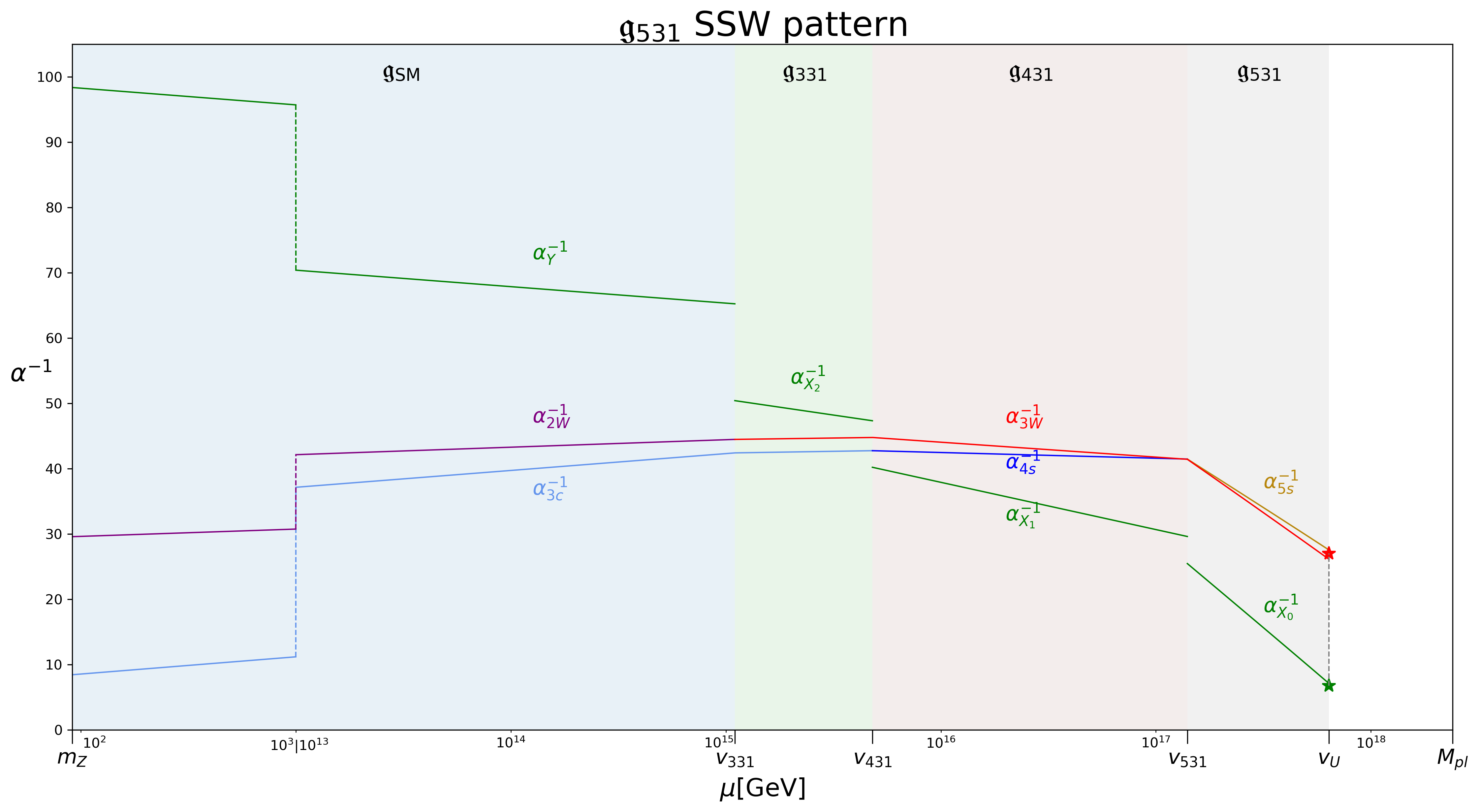
Figure 1: The two-loop RGEs of the ${\mathfrak{s}\mathfrak{u}}(8)$ setup according to the SSW symmetry breaking pattern. The RG evolutions within $10^{3}\,{\rm GeV}\lesssim\mu\lesssim 10^{13}\,{\rm GeV}$ are zoomed out in order to highlight the behaviors in three intermediate symmetry breaking scales given by the benchmark point in Eq. (115).

With the one- and two-loop $\beta$ coefficients defined in Eqs. (2.3), (2.3), (2.3), and (2.3), we plot the RGEs of the ${\mathfrak{s}\mathfrak{u}}(8)$ setup along the SSW symmetry breaking pattern in Fig. 1. The discontinuities of the ${\mathfrak{u}}(1)$ gauge couplings at three intermediate scales follow from their definitions in Eqs. (25), (28), (31), respectively. The benchmark point in Fig. 1 is marked by $\star$ and reads

$$c_{\rm HSW}\approx-0.38\,,\penalty 10000\ v_{U}\approx 6.39\times 10^{17}\,{\rm GeV}\,,$$

$$\alpha_{5c}^{-1}(v_{U})\approx 27.55\,,\penalty 10000\ \alpha_{3W}^{-1}(v_{U})\approx 26.13\,,\penalty 10000\ \alpha_{X_{0}}^{-1}(v_{U})\approx 7.11\,.$$ (32)

3 The SWS symmetry breaking pattern

3.1 Decompositions of the ${\mathfrak{s}\mathfrak{u}}$(8) fermions

${\mathfrak{s}\mathfrak{u}}(8)$	$\mathfrak{g}_{531}$	$\mathfrak{g}_{431}$	$\mathfrak{g}_{421}$	$\mathfrak{g}_{\rm SM}$
$\mathbf{\overline{8_{F}}}^{\Omega}$	$(\mathbf{\overline{5}}\,,\mathbf{1}\,,+\frac{1}{5})_{\mathbf{F}}^{\Omega}$	$(\mathbf{\overline{4}}\,,\mathbf{1}\,,+\frac{1}{4})_{\mathbf{F}}^{\Omega}$	$(\mathbf{\overline{4}}\,,\mathbf{1}\,,+\frac{1}{4})_{\mathbf{F}}^{\Omega}$	$(\mathbf{\overline{3}}\,,\mathbf{1}\,,+\frac{1}{3})_{\mathbf{F}}^{\Omega}\penalty 10000\ :\penalty 10000\ {\mathcal{D}_{R}^{\Omega}}^{c}$
				$(\mathbf{1}\,,\mathbf{1}\,,0)_{\mathbf{F}}^{\Omega}\penalty 10000\ :\penalty 10000\ \check{\mathcal{N}}_{L}^{\Omega}$
		$(\mathbf{1}\,,\mathbf{1}\,,0)_{\mathbf{F}}^{\Omega^{\prime}}$	$(\mathbf{1}\,,\mathbf{1}\,,0)_{\mathbf{F}}^{\Omega^{\prime}}$	$(\mathbf{1}\,,\mathbf{1}\,,0)_{\mathbf{F}}^{\Omega^{\prime}}\penalty 10000\ :\penalty 10000\ \check{\mathcal{N}}_{L}^{\Omega^{\prime}}$
	$(\mathbf{1}\,,\mathbf{\overline{3}}\,,-\frac{1}{3})_{\mathbf{F}}^{\Omega}$	$(\mathbf{1}\,,\mathbf{\overline{3}}\,,-\frac{1}{3})_{\mathbf{F}}^{\Omega}$	$(\mathbf{1}\,,\mathbf{\overline{2}}\,,-\frac{1}{2})_{\mathbf{F}}^{\Omega}$	$(\mathbf{1}\,,\mathbf{\overline{2}}\,,-\frac{1}{2})_{\mathbf{F}}^{\Omega}\penalty 10000\ :\penalty 10000\ \mathcal{L}_{L}^{\Omega}=(\mathcal{E}_{L}^{\Omega}\,,-\mathcal{N}_{L}^{\Omega})^{T}$
			$(\mathbf{1}\,,\mathbf{1}\,,0)_{\mathbf{F}}^{\Omega^{\prime\prime}}$	$(\mathbf{1}\,,\mathbf{1}\,,0)_{\mathbf{F}}^{\Omega^{\prime\prime}}\penalty 10000\ :\penalty 10000\ \check{\mathcal{N}}_{L}^{\Omega^{\prime\prime}}$

Table 5: The ${\mathfrak{s}\mathfrak{u}}(8)$ fermion representation of $\mathbf{\overline{8_{F}}}^{\Omega}$ under the $\mathfrak{g}_{531}\,,\mathfrak{g}_{431}\,,\mathfrak{g}_{421}\,,\mathfrak{g}_{\rm SM}$ subalgebras.

${\mathfrak{s}\mathfrak{u}}(8)$	$\mathfrak{g}_{531}$	$\mathfrak{g}_{431}$	$\mathfrak{g}_{421}$	$\mathfrak{g}_{\rm SM}$
$\mathbf{28_{F}}$	$(\mathbf{1}\,,\mathbf{\overline{3}}\,,+\frac{2}{3})_{\mathbf{F}}$	$(\mathbf{1}\,,\mathbf{\overline{3}}\,,+\frac{2}{3})_{\mathbf{F}}$	$(\mathbf{1}\,,\mathbf{\overline{2}}\,,+\frac{1}{2})_{\mathbf{F}}$	$(\mathbf{1}\,,\mathbf{\overline{2}}\,,+\frac{1}{2})_{\mathbf{F}}\penalty 10000\ :\penalty 10000\ ({\mathfrak{n}_{R}}^{c}\,,-{\mathfrak{e}_{R}}^{c})^{T}$
			$(\mathbf{1}\,,\mathbf{1}\,,+1)_{\mathbf{F}}$	$\underline{(\mathbf{1}\,,\mathbf{1}\,,+1)_{\mathbf{F}}\penalty 10000\ :\penalty 10000\ {\tau_{R}}^{c}}$
	$(\mathbf{5}\,,\mathbf{3}\,,+\frac{2}{15})_{\mathbf{F}}$	$(\mathbf{1}\,,\mathbf{3}\,,+\frac{1}{3})_{\mathbf{F}}^{\prime}$	$(\mathbf{1}\,,\mathbf{2}\,,+\frac{1}{2})_{\mathbf{F}}^{\prime}$	$(\mathbf{1}\,,\mathbf{2}\,,+\frac{1}{2})_{\mathbf{F}}^{\prime}\penalty 10000\ :\penalty 10000\ ({\mathfrak{e}_{R}^{\prime}}^{c}\,,{\mathfrak{n}_{R}^{\prime}}^{c})^{T}$
			$(\mathbf{1}\,,\mathbf{1}\,,0)_{\mathbf{F}}$	$(\mathbf{1}\,,\mathbf{1}\,,0)_{\mathbf{F}}\penalty 10000\ :\penalty 10000\ \check{\mathfrak{n}}_{R}^{c}$
		$(\mathbf{4}\,,\mathbf{3}\,,+\frac{1}{12})_{\mathbf{F}}$	$(\mathbf{4}\,,\mathbf{1}\,,-\frac{1}{4})_{\mathbf{F}}$	$(\mathbf{3}\,,\mathbf{1}\,,-\frac{1}{3})_{\mathbf{F}}\penalty 10000\ :\penalty 10000\ \mathfrak{D}_{L}$
				$(\mathbf{1}\,,\mathbf{1}\,,0)_{\mathbf{F}}^{\prime}\penalty 10000\ :\penalty 10000\ \check{\mathfrak{n}}_{R}^{\prime\,c}$
			$(\mathbf{4}\,,\mathbf{2}\,,+\frac{1}{4})_{\mathbf{F}}$	$(\mathbf{1}\,,\mathbf{2}\,,+\frac{1}{2})_{\mathbf{F}}^{\prime\prime}\penalty 10000\ :\penalty 10000\ ({\mathfrak{e}_{R}^{\prime\prime}}^{c}\,,{\mathfrak{n}_{R}^{\prime\prime}}^{c})^{T}$
				$\underline{(\mathbf{3}\,,\mathbf{2}\,,+\frac{1}{6})_{\mathbf{F}}\penalty 10000\ :\penalty 10000\ (t_{L}\,,b_{L})^{T}}$
	$(\mathbf{10}\,,\mathbf{1}\,,-\frac{2}{5})_{\mathbf{F}}$	$(\mathbf{4}\,,\mathbf{1}\,,-\frac{1}{4})_{\mathbf{F}}^{\prime}$	$(\mathbf{4}\,,\mathbf{1}\,,-\frac{1}{4})_{\mathbf{F}}^{\prime}$	$(\mathbf{3}\,,\mathbf{1}\,,-\frac{1}{3})_{\mathbf{F}}^{\prime}\penalty 10000\ :\penalty 10000\ \mathfrak{D}_{L}^{\prime}$
				$(\mathbf{1}\,,\mathbf{1}\,,0)_{\mathbf{F}}^{\prime\prime}\penalty 10000\ :\penalty 10000\ \check{\mathfrak{n}}_{R}^{\prime\prime\,c}$
		$(\mathbf{6}\,,\mathbf{1}\,,-\frac{1}{2})_{\mathbf{F}}$	$(\mathbf{6}\,,\mathbf{1}\,,-\frac{1}{2})_{\mathbf{F}}$	$(\mathbf{3}\,,\mathbf{1}\,,-\frac{1}{3})_{\mathbf{F}}^{\prime\prime}\penalty 10000\ :\penalty 10000\ \mathfrak{D}_{L}^{\prime\prime}$
				$\underline{(\mathbf{\overline{3}}\,,\mathbf{1}\,,-\frac{2}{3})_{\mathbf{F}}\penalty 10000\ :\penalty 10000\ {t_{R}}^{c}}$

Table 6: The ${\mathfrak{s}\mathfrak{u}}(8)$ fermion representation of $\mathbf{28_{F}}$ under the $\mathfrak{g}_{531}\,,\mathfrak{g}_{431}\,,\mathfrak{g}_{421}\,,\mathfrak{g}_{\rm SM}$ subalgebras. All IRs for SM fermions are marked with underlines.

${\mathfrak{s}\mathfrak{u}}(8)$	$\mathfrak{g}_{531}$	$\mathfrak{g}_{431}$	$\mathfrak{g}_{421}$	$\mathfrak{g}_{\rm SM}$
$\mathbf{56_{F}}$	$(\mathbf{1}\,,\mathbf{1}\,,+1)_{\mathbf{F}}^{\prime}$	$(\mathbf{1}\,,\mathbf{1}\,,+1)_{\mathbf{F}}^{\prime}$	$(\mathbf{1}\,,\mathbf{1}\,,+1)_{\mathbf{F}}^{\prime}$	$\underline{(\mathbf{1}\,,\mathbf{1}\,,+1)_{\mathbf{F}}^{\prime}\penalty 10000\ :\penalty 10000\ {\mu_{R}}^{c}}$
	$(\mathbf{5}\,,\mathbf{\overline{3}}\,,+\frac{7}{15})_{\mathbf{F}}$	$(\mathbf{1}\,,\mathbf{\overline{3}}\,,+\frac{2}{3})_{\mathbf{F}}^{\prime}$	$(\mathbf{1}\,,\mathbf{\overline{2}}\,,+\frac{1}{2})_{\mathbf{F}}^{\prime\prime\prime}$	$(\mathbf{1}\,,\mathbf{\overline{2}}\,,+\frac{1}{2})_{\mathbf{F}}^{\prime\prime\prime}\penalty 10000\ :\penalty 10000\ ({\mathfrak{n}_{R}^{\prime\prime\prime}}^{c}\,,-{\mathfrak{e}_{R}^{\prime\prime\prime}}^{c})^{T}$
			$(\mathbf{1}\,,\mathbf{1}\,,+1)_{\mathbf{F}}^{\prime\prime}$	$\underline{(\mathbf{1}\,,\mathbf{1}\,,+1)_{\mathbf{F}}^{\prime\prime}\penalty 10000\ :\penalty 10000\ {e_{R}}^{c}}$
		$(\mathbf{4}\,,\mathbf{\overline{3}}\,,+\frac{5}{12})_{\mathbf{F}}$	$(\mathbf{4}\,,\mathbf{1}\,,+\frac{3}{4})_{\mathbf{F}}$	$(\mathbf{3}\,,\mathbf{1}\,,+\frac{2}{3})_{\mathbf{F}}\penalty 10000\ :\penalty 10000\ \mathfrak{U}_{L}$
				$(\mathbf{1}\,,\mathbf{1}\,,+1)_{\mathbf{F}}^{\prime\prime\prime}\penalty 10000\ :\penalty 10000\ {\mathfrak{E}_{R}}^{c}$
			$(\mathbf{4}\,,\mathbf{\overline{2}}\,,+\frac{1}{4})_{\mathbf{F}}$	$(\mathbf{3}\,,\mathbf{\overline{2}}\,,+\frac{1}{6})_{\mathbf{F}}\penalty 10000\ :\penalty 10000\ (\mathfrak{d}_{L}\,,-\mathfrak{u}_{L})^{T}$
				$(\mathbf{1}\,,\mathbf{\overline{2}}\,,+\frac{1}{2})_{\mathbf{F}}^{\prime\prime\prime\prime}\penalty 10000\ :\penalty 10000\ ({\mathfrak{n}_{R}^{\prime\prime\prime\prime}}^{c}\,,-{\mathfrak{e}_{R}^{\prime\prime\prime\prime}}^{c})^{T}$
	$(\mathbf{\overline{10}}\,,\mathbf{1}\,,-\frac{3}{5})_{\mathbf{F}}$	$(\mathbf{\overline{4}}\,,\mathbf{1}\,,-\frac{3}{4})_{\mathbf{F}}$	$(\mathbf{\overline{4}}\,,\mathbf{1}\,,-\frac{3}{4})_{\mathbf{F}}$	$(\mathbf{1}\,,\mathbf{1}\,,-1)_{\mathbf{F}}\penalty 10000\ :\penalty 10000\ \mathfrak{E}_{L}$
				$(\mathbf{\overline{3}}\,,\mathbf{1}\,,-\frac{2}{3})_{\mathbf{F}}^{\prime}\penalty 10000\ :\penalty 10000\ {\mathfrak{U}_{R}}^{c}$
		$(\mathbf{6}\,,\mathbf{1}\,,-\frac{1}{2})_{\mathbf{F}}^{\prime}$	$(\mathbf{6}\,,\mathbf{1}\,,-\frac{1}{2})_{\mathbf{F}}^{\prime}$	$(\mathbf{3}\,,\mathbf{1}\,,-\frac{1}{3})_{\mathbf{F}}^{\prime\prime\prime}\penalty 10000\ :\penalty 10000\ \mathfrak{D}_{L}^{\prime\prime\prime}$
				$\underline{(\mathbf{\overline{3}}\,,\mathbf{1}\,,-\frac{2}{3})_{\mathbf{F}}^{\prime\prime}\penalty 10000\ :\penalty 10000\ {u_{R}}^{c}}$
	$(\mathbf{10}\,,\mathbf{3}\,,-\frac{1}{15})_{\mathbf{F}}$	$(\mathbf{4}\,,\mathbf{3}\,,+\frac{1}{12})_{\mathbf{F}}^{\prime}$	$(\mathbf{4}\,,\mathbf{1}\,,-\frac{1}{4})_{\mathbf{F}}^{\prime\prime}$	$(\mathbf{3}\,,\mathbf{1}\,,-\frac{1}{3})_{\mathbf{F}}^{\prime\prime\prime\prime}\penalty 10000\ :\penalty 10000\ \mathfrak{D}_{L}^{\prime\prime\prime\prime}$
				$(\mathbf{1}\,,\mathbf{1}\,,0)_{\mathbf{F}}^{\prime\prime\prime}\penalty 10000\ :\penalty 10000\ {\check{\mathfrak{n}}_{R}}^{\prime\prime\prime\,c}$
			$(\mathbf{4}\,,\mathbf{2}\,,+\frac{1}{4})_{\mathbf{F}}^{\prime}$	$\underline{(\mathbf{3}\,,\mathbf{2}\,,+\frac{1}{6})_{\mathbf{F}}^{\prime}\penalty 10000\ :\penalty 10000\ (u_{L}\,,d_{L})^{T}}$
				$(\mathbf{1}\,,\mathbf{2}\,,+\frac{1}{2})_{\mathbf{F}}^{\prime\prime\prime\prime\prime}\penalty 10000\ :\penalty 10000\ ({\mathfrak{e}_{R}^{\prime\prime\prime\prime\prime}}^{c}\,,{\mathfrak{n}_{R}^{\prime\prime\prime\prime\prime}}^{c})^{T}$
		$(\mathbf{6}\,,\mathbf{3}\,,-\frac{1}{6})_{\mathbf{F}}$	$(\mathbf{6}\,,\mathbf{1}\,,-\frac{1}{2})_{\mathbf{F}}^{\prime\prime}$	$(\mathbf{3}\,,\mathbf{1}\,,-\frac{1}{3})_{\mathbf{F}}^{\prime\prime\prime\prime\prime}\penalty 10000\ :\penalty 10000\ \mathfrak{D}_{L}^{\prime\prime\prime\prime\prime}$
				$\underline{(\mathbf{\overline{3}}\,,\mathbf{1}\,,-\frac{2}{3})_{\mathbf{F}}^{\prime\prime\prime}\penalty 10000\ :\penalty 10000\ {c_{R}}^{c}}$
			$(\mathbf{6}\,,\mathbf{2}\,,0)_{\mathbf{F}}$	$\underline{(\mathbf{3}\,,\mathbf{2}\,,+\frac{1}{6})_{\mathbf{F}}^{\prime\prime}\penalty 10000\ :\penalty 10000\ (c_{L}\,,s_{L})^{T}}$
				$(\mathbf{\overline{3}}\,,\mathbf{2}\,,-\frac{1}{6})_{\mathbf{F}}\penalty 10000\ :\penalty 10000\ ({\mathfrak{d}_{R}}^{c}\,,{\mathfrak{u}_{R}}^{c})^{T}$

Table 7: The ${\mathfrak{s}\mathfrak{u}}(8)$ fermion representation of $\mathbf{56_{F}}$ under the $\mathfrak{g}_{531}\,,\mathfrak{g}_{431}\,,\mathfrak{g}_{421}\,,\mathfrak{g}_{\rm SM}$ subalgebras. All IRs for SM fermions are marked with underlines.

By following the SWS symmetry breaking pattern in Eq. (13b), we tabulate the fermion representations at various stages in Tables 5, 6, and 7. Along this pattern, the global $\widetilde{{\rm U}}(1)_{T}$ symmetry evolves to the global $\widetilde{{\rm U}}(1)_{B-L}$ at the EW scale according to the following sequence:

$$\mathfrak{g}_{531}\penalty 10000\ :\penalty 10000\ \mathcal{T}^{\prime}\equiv\mathcal{T}-5t\mathcal{X}_{0}\,,\quad\mathfrak{g}_{431}\penalty 10000\ :\penalty 10000\ \mathcal{T}^{\prime\prime}\equiv\mathcal{T}^{\prime}+8t\mathcal{X}_{1}\,,$$

$$\mathfrak{g}_{421}\penalty 10000\ :\penalty 10000\ \mathcal{T}^{\prime\prime\prime}\equiv\mathcal{T}^{\prime\prime}-8t\mathcal{X}_{2}\,,\quad\mathfrak{g}_{\rm SM}\penalty 10000\ :\penalty 10000\ \mathcal{B}-\mathcal{L}\equiv\mathcal{T}^{\prime\prime\prime}+8t\mathcal{Y}\,.$$ (33)

3.2 Decompositions of the ${\mathfrak{s}\mathfrak{u}}$(8) Higgs fields

We decompose the Higgs fields in Eq. (6) into components that can be responsible for the sequential symmetry breaking stages in Eq. (13b). For Higgs fields of $\mathbf{\overline{8_{H}}}_{\,,\omega}$, they read

$$\mathbf{\overline{8_{H}}}_{\,,\omega} \supset \underline{(\mathbf{1}\,,\mathbf{\overline{3}}\,,-\frac{1}{3})_{\mathbf{H}\,,\omega}}\oplus\langle(\mathbf{\overline{5}}\,,\mathbf{1}\,,+\frac{1}{5})_{\mathbf{H}\,,\omega}\rangle$$ (34)

$$\supset \langle(\mathbf{1}\,,\mathbf{\overline{3}}\,,-\frac{1}{3})_{\mathbf{H}\,,\omega}\rangle\oplus\underline{(\mathbf{\overline{4}}\,,\mathbf{1}\,,+\frac{1}{4})_{\mathbf{H}\,,\omega}}$$

$$\supset \langle(\mathbf{\overline{4}}\,,\mathbf{1}\,,+\frac{1}{4})_{\mathbf{H}\,,\omega}\rangle\,.$$

For Higgs fields of $\mathbf{\overline{28_{H}}}_{\,,\dot{\omega}}$, they read

$$\mathbf{\overline{28_{H}}}_{\,,\dot{\omega}} \supset \underline{(\mathbf{1}\,,\mathbf{3}\,,-\frac{2}{3})_{\mathbf{H}\,,\dot{\omega}}}\oplus\underline{(\mathbf{\overline{5}}\,,\mathbf{\overline{3}}\,,-\frac{2}{15})_{\mathbf{H}\,,\dot{\omega}}}\oplus\underline{(\mathbf{\overline{10}}\,,\mathbf{1}\,,+\frac{2}{5})_{\mathbf{H}\,,\dot{\omega}}}$$ (35)

$$\supset \underline{(\mathbf{1}\,,\mathbf{3}\,,-\frac{2}{3})_{\mathbf{H}\,,\dot{\omega}}}\oplus\Big[\langle(\mathbf{1}\,,\mathbf{\overline{3}}\,,-\frac{1}{3})_{\mathbf{H}\,,\dot{\omega}}\rangle\oplus\underline{(\mathbf{\overline{4}}\,,\mathbf{\overline{3}}\,,-\frac{1}{12})_{\mathbf{H}\,,\dot{\omega}}}\Big]\oplus\underline{(\mathbf{\overline{4}}\,,\mathbf{1}\,,+\frac{1}{4})_{\mathbf{H}\,,\dot{\omega}}}$$

$$\supset \underline{(\mathbf{1}\,,\mathbf{2}\,,-\frac{1}{2})_{\mathbf{H}\,,\dot{\omega}}}\oplus\Big[\underline{(\mathbf{1}\,,\mathbf{\overline{2}}\,,-\frac{1}{2})_{\mathbf{H}\,,\dot{\omega}}}\oplus\langle(\mathbf{\overline{4}}\,,\mathbf{1}\,,+\frac{1}{4})_{\mathbf{H}\,,\dot{\omega}}\rangle\oplus\underline{(\mathbf{\overline{4}}\,,\mathbf{\overline{2}}\,,-\frac{1}{4})_{\mathbf{H}\,,\dot{\omega}}}\Big]$$

$$\oplus \langle(\mathbf{\overline{4}}\,,\mathbf{1}\,,+\frac{1}{4})_{\mathbf{H}\,,\dot{\omega}}^{\prime}\rangle\,.$$

For Higgs field of $\mathbf{70_{H}}$, it reads

$$\mathbf{70_{H}} \supset (\mathbf{5}\,,\mathbf{1}\,,+\frac{4}{5})_{\mathbf{H}}\oplus(\mathbf{\overline{5}}\,,\mathbf{1}\,,-\frac{4}{5})_{\mathbf{H}}\oplus\underline{(\mathbf{10}\,,\mathbf{\overline{3}}\,,+\frac{4}{15})_{\mathbf{H}}}\oplus(\mathbf{\overline{10}}\,,\mathbf{3}\,,-\frac{4}{15})_{\mathbf{H}}$$ (36)

$$\supset \underline{(\mathbf{4}\,,\mathbf{\overline{3}}\,,+\frac{5}{12})_{\mathbf{H}}}\supset\underline{(\mathbf{4}\,,\mathbf{\overline{2}}\,,+\frac{1}{4})_{\mathbf{H}}}\supset\langle(\mathbf{1}\,,\mathbf{\overline{2}}\,,+\frac{1}{2})_{\mathbf{H}}\rangle\,.$$

3.3 RGEs of the SWS symmetry breaking pattern

Between the $v_{531}\leq\mu\leq v_{U}$, almost all massless Higgs fields are in the first lines of Eq. (34), (35) and Eq. (36), which are

$$(\mathbf{\overline{5}}\,,\mathbf{1}\,,+\frac{1}{5})_{\mathbf{H}\,,\omega}\oplus(\mathbf{1}\,,\mathbf{\overline{3}}\,,-\frac{1}{3})_{\mathbf{H}\,,\omega}\subset\mathbf{\overline{8_{H}}}_{\,,\omega}\,,$$

$$(\mathbf{1}\,,\mathbf{3}\,,-\frac{2}{3})_{\mathbf{H}\,,\dot{\omega}}\oplus(\mathbf{\overline{5}}\,,\mathbf{\overline{3}}\,,-\frac{2}{15})_{\mathbf{H}\,,\dot{\omega}}\oplus(\mathbf{\overline{10}}\,,\mathbf{1}\,,+\frac{2}{5})_{\mathbf{H}\,,\dot{\omega}}\subset\mathbf{\overline{28_{H}}}_{\,,\dot{\omega}}\,,$$

$$(\mathbf{5}\,,\mathbf{1}\,,+\frac{4}{5})_{\mathbf{H}}\oplus(\mathbf{\overline{5}}\,,\mathbf{1}\,,-\frac{4}{5})_{\mathbf{H}}\oplus(\mathbf{10}\,,\mathbf{\overline{3}}\,,+\frac{4}{15})_{\mathbf{H}}\oplus(\mathbf{\overline{10}}\,,\mathbf{3}\,,-\frac{4}{15})_{\mathbf{H}}\subset\mathbf{70_{H}}\,,$$

$$(\mathbf{\overline{5}}\,,\mathbf{1}\,,-\frac{4}{5})_{\mathbf{H}}\oplus(\mathbf{5}\,,\mathbf{1}\,,+\frac{4}{5})_{\mathbf{H}}\oplus(\mathbf{\overline{10}}\,,\mathbf{3}\,,-\frac{4}{15})_{\mathbf{H}}\oplus(\mathbf{10}\,,\mathbf{\overline{3}}\,,+\frac{4}{15})_{\mathbf{H}}\subset\mathbf{\overline{70_{H}}}\,,$$

$$(\mathbf{5}\,,\mathbf{1}\,,-\frac{1}{5})_{\mathbf{H}}^{\omega}\oplus(\mathbf{1}\,,\mathbf{3}\,,+\frac{1}{3})_{\mathbf{H}}^{\omega}\subset\mathbf{8_{H}}^{\omega}\,,$$

$$(\mathbf{1}\,,\mathbf{\overline{3}}\,,+\frac{2}{3})_{\mathbf{H}}^{\dot{\omega}}\oplus(\mathbf{5}\,,\mathbf{3}\,,+\frac{2}{15})_{\mathbf{H}}^{\dot{\omega}}\oplus(\mathbf{10}\,,\mathbf{1}\,,-\frac{2}{5})_{\mathbf{H}}^{\dot{\omega}}\subset\mathbf{28_{H}}^{\dot{\omega}}\,.$$ (37)

All fermionic components of $\mathbf{\overline{8_{F}}}^{\Omega}\oplus\mathbf{28_{F}}\oplus\mathbf{56_{F}}$ remain massless after the decomposition into the $\mathfrak{g}_{531}$ IRs. Consequently, we have the $\mathfrak{g}_{531}$ $\beta$ coefficients of

$$(b^{(1)}_{{\mathfrak{s}\mathfrak{u}}(5)_{s}}\,,b^{(1)}_{{\mathfrak{s}\mathfrak{u}}(3)_{W}}\,,b^{(1)}_{{\mathfrak{u}}(1)_{X_{0}}})=(+54\,,+60\,,+\frac{368}{5})\,,$$

$$b^{(2)}_{\mathfrak{g}_{531}}=\begin{pmatrix}6984/5&216&672/25\\ 648&728&352/15\\ 16128/25&2816/15&98816/1125\end{pmatrix}\,.$$ (38)

Between the $v_{431}\leq\mu\leq v_{531}$, the massless Higgs fields are the following:

$$(\mathbf{\overline{4}}\,,\mathbf{1}\,,+\frac{1}{4})_{\mathbf{H}\,,3,\rm V,\rm VI}\oplus(\mathbf{1}\,,\mathbf{\overline{3}}\,,-\frac{1}{3})_{\mathbf{H}\,,3,\rm V,\rm VI}\subset...\subset\mathbf{\overline{8_{H}}}_{\,,3,\rm V,\rm VI}\,,$$ (39)

$$(\mathbf{1}\,,\mathbf{3}\,,-\frac{2}{3})_{\mathbf{H}\,,\dot{\omega}}\oplus\Big[(\mathbf{\overline{4}}\,,\mathbf{1}\,,+\frac{1}{4})_{\mathbf{H}\,,\dot{\omega}}\oplus(\mathbf{6}\,,\mathbf{1}\,,+\frac{1}{2})_{\mathbf{H}\,,\dot{\omega}}\Big]$$

$$\oplus \Big[(\mathbf{1}\,,\mathbf{\overline{3}}\,,-\frac{1}{3})_{\mathbf{H}\,,\dot{\omega}}\oplus(\mathbf{\overline{4}}\,,\mathbf{\overline{3}}\,,-\frac{1}{12})_{\mathbf{H}\,,\dot{\omega}}\Big]\subset...\subset\mathbf{\overline{28_{H}}}_{\,,\dot{\omega}}\,,\quad\dot{\omega}=(\dot{1},\dot{2},\dot{\rm VII},\dot{\rm VIII},\dot{\rm IX})\,,$$

$$(\mathbf{1}\,,\mathbf{\overline{3}}\,,+\frac{2}{3})_{\mathbf{H}}^{\dot{\rm\kappa}}\oplus\Big[(\mathbf{1}\,,\mathbf{3}\,,+\frac{1}{3})_{\mathbf{H}}^{\dot{\rm\kappa}}\oplus(\mathbf{4}\,,\mathbf{3}\,,+\frac{1}{12})_{\mathbf{H}}^{\dot{\rm\kappa}}\Big]$$

$$\oplus \Big[(\mathbf{4}\,,\mathbf{1}\,,-\frac{1}{4})_{\mathbf{H}}^{\dot{\rm\kappa}}\oplus(\mathbf{6}\,,\mathbf{1}\,,-\frac{1}{2})_{\mathbf{H}}^{\dot{\rm\kappa}}\Big]\subset...\subset\mathbf{28_{H}}^{\dot{\rm\kappa}}\,,\quad\dot{\kappa}=(\dot{\rm VII},\dot{\rm IX})\,,$$

$$(\mathbf{4}\,,\mathbf{\overline{3}}\,,+\frac{5}{12})_{\mathbf{H}}\subset...\subset\mathbf{70_{H}}\,.$$

All ${\mathfrak{s}\mathfrak{u}}$(8) fermions in Eq. (119) remain massless after the decomposition into the $\mathfrak{g}_{431}$ IRs. Consequently, we have the $\mathfrak{g}_{431}$ $\beta$ coefficients of

$$(b^{(1)}_{{\mathfrak{s}\mathfrak{u}}(4)_{s}}\,,b^{(1)}_{{\mathfrak{s}\mathfrak{u}}(3)_{W}}\,,b^{(1)}_{{\mathfrak{u}}(1)_{X_{1}}})=(+\frac{8}{3}\,,+\frac{13}{2}\,,+\frac{61}{3})\,,$$

$$b^{(2)}_{\mathfrak{g}_{431}}=\begin{pmatrix}3907/12&84&99/8\\ 315/2&255&155/12\\ 1485/8&310/3&5855/144\end{pmatrix}\,.$$ (40)

The ${\mathfrak{s}\mathfrak{u}}(5)_{s}\oplus{\mathfrak{u}}(1)_{X_{0}}$ gauge couplings match with the ${\mathfrak{s}\mathfrak{u}}(4)_{s}\oplus{\mathfrak{u}}(1)_{X_{1}}$ gauge couplings as follows:

$$\alpha_{5s}^{-1}(v_{531})=\alpha_{4s}^{-1}(v_{531})\,,\penalty 10000\ \alpha_{X_{1}}^{-1}(v_{531})=\frac{1}{10}\alpha_{5s}^{-1}(v_{531})+\alpha_{X_{0}}^{-1}(v_{531})\,.$$ (41)

Between the $v_{421}\leq\mu\leq v_{431}$, the massless Higgs fields are

$$(\mathbf{\overline{4}}\,,\mathbf{1}\,,+\frac{1}{4})_{\mathbf{H}\,,3,\rm VI}\oplus(\mathbf{1}\,,\mathbf{\overline{2}}\,,-\frac{1}{2})_{\mathbf{H}\,,3,\rm VI}\subset...\subset\mathbf{\overline{8_{H}}}_{,3,\rm VI}\,,$$ (42)

$$\Big[(\mathbf{1}\,,\mathbf{2}\,,-\frac{1}{2})_{\mathbf{H}\,,\dot{\omega}}\oplus(\mathbf{1}\,,\mathbf{1}\,,-1)_{\mathbf{H}\,,\dot{\omega}}\Big]\oplus\Big[(\mathbf{\overline{4}}\,,\mathbf{1}\,,+\frac{1}{4})_{\mathbf{H}\,,\dot{\omega}}^{\prime}\oplus(\mathbf{6}\,,\mathbf{1}\,,+\frac{1}{2})_{\mathbf{H}\,,\dot{\omega}}\Big]$$

$$\oplus \Big[(\mathbf{1}\,,\mathbf{\overline{2}}\,,-\frac{1}{2})_{\mathbf{H}\,,\dot{\omega}}\oplus(\mathbf{\overline{4}}\,,\mathbf{1}\,,+\frac{1}{4})_{\mathbf{H}\,,\dot{\omega}}\oplus(\mathbf{\overline{4}}\,,\mathbf{\overline{2}}\,,-\frac{1}{4})_{\mathbf{H}\,,\dot{\omega}}\Big]\subset...\subset\mathbf{\overline{28_{H}}}_{\,,\dot{\omega}}\,,\quad\dot{\omega}=(\dot{2},\dot{\rm VIII},\dot{\rm IX})\,,$$

$$\Big[(\mathbf{1}\,,\mathbf{\overline{2}}\,,+\frac{1}{2})_{\mathbf{H}}^{\dot{\rm IX}}\oplus(\mathbf{1}\,,\mathbf{1}\,,+1)_{\mathbf{H}}^{\dot{\rm IX}}\Big]\oplus\Big[(\mathbf{4}\,,\mathbf{1}\,,-\frac{1}{4})_{\mathbf{H}}^{\dot{\rm IX}^{\prime}}\oplus(\mathbf{6}\,,\mathbf{1}\,,-\frac{1}{2})_{\mathbf{H}}^{\dot{\rm IX}}\Big]$$

$$\oplus \Big[(\mathbf{1}\,,\mathbf{2}\,,+\frac{1}{2})_{\mathbf{H}}^{\dot{\rm IX}}\oplus(\mathbf{4}\,,\mathbf{1}\,,-\frac{1}{4})_{\mathbf{H}}^{\dot{\rm IX}}\oplus(\mathbf{4}\,,\mathbf{2}\,,+\frac{1}{4})_{\mathbf{H}}^{\dot{\rm IX}}\Big]\subset...\subset\mathbf{28_{H}}^{\dot{\rm IX}}\,,$$

$$(\mathbf{4}\,,\mathbf{\overline{2}}\,,+\frac{1}{4})_{\mathbf{H}}\subset...\subset\mathbf{70_{H}}\,.$$

All ${\mathfrak{s}\mathfrak{u}}$(8) fermions in Eq. (123) remain massless after the decomposition into the $\mathfrak{g}_{421}$ IRs. Consequently, we have the $\mathfrak{g}_{421}$ $\beta$ coefficients of

$$(b^{(1)}_{{\mathfrak{s}\mathfrak{u}}(4)_{s}}\,,b^{(1)}_{{\mathfrak{s}\mathfrak{u}}(2)_{W}}\,,b^{(1)}_{{\mathfrak{u}}(1)_{X_{2}}})=(-\frac{8}{3}\,,+\frac{17}{3}\,,+\frac{47}{3})\,,$$

$$b^{(2)}_{\mathfrak{g}_{421}}=\begin{pmatrix}991/6&45/2&35/4\\ 225/2&353/3&39/4\\ 525/4&117/4&307/8\end{pmatrix}\,.$$ (43)

The ${\mathfrak{s}\mathfrak{u}}(3)_{W}\oplus{\mathfrak{u}}(1)_{X_{1}}$ gauge couplings match with the ${\mathfrak{s}\mathfrak{u}}(2)_{W}\oplus{\mathfrak{u}}(1)_{X_{2}}$ gauge couplings as follows:

$$\alpha_{3W}^{-1}(v_{431})=\alpha_{2W}^{-1}(v_{431})\,,\penalty 10000\ \alpha_{X_{2}}^{-1}(v_{431})=\frac{1}{3}\alpha_{3W}^{-1}(v_{431})+\alpha_{X_{1}}^{-1}(v_{431})\,.$$ (44)

Between the $v_{\rm EW}\leq\mu\leq v_{421}$, we have the same $\mathfrak{g}_{\rm SM}$ $\beta$ coefficients as Eq. (2.3). The ${\mathfrak{s}\mathfrak{u}}(4)_{s}\oplus{\mathfrak{u}}(1)_{X_{2}}$ gauge couplings match with the ${\mathfrak{s}\mathfrak{u}}(3)_{c}\oplus{\mathfrak{u}}(1)_{Y}$ gauge couplings as follows:

$$\alpha_{4s}^{-1}(v_{421})=\alpha_{3c}^{-1}(v_{421})\,,\penalty 10000\ \alpha_{\rm Y}^{-1}(v_{421})=\frac{1}{6}\alpha_{4s}^{-1}(v_{421})+\alpha_{X_{2}}^{-1}(v_{421})\,.$$ (45)

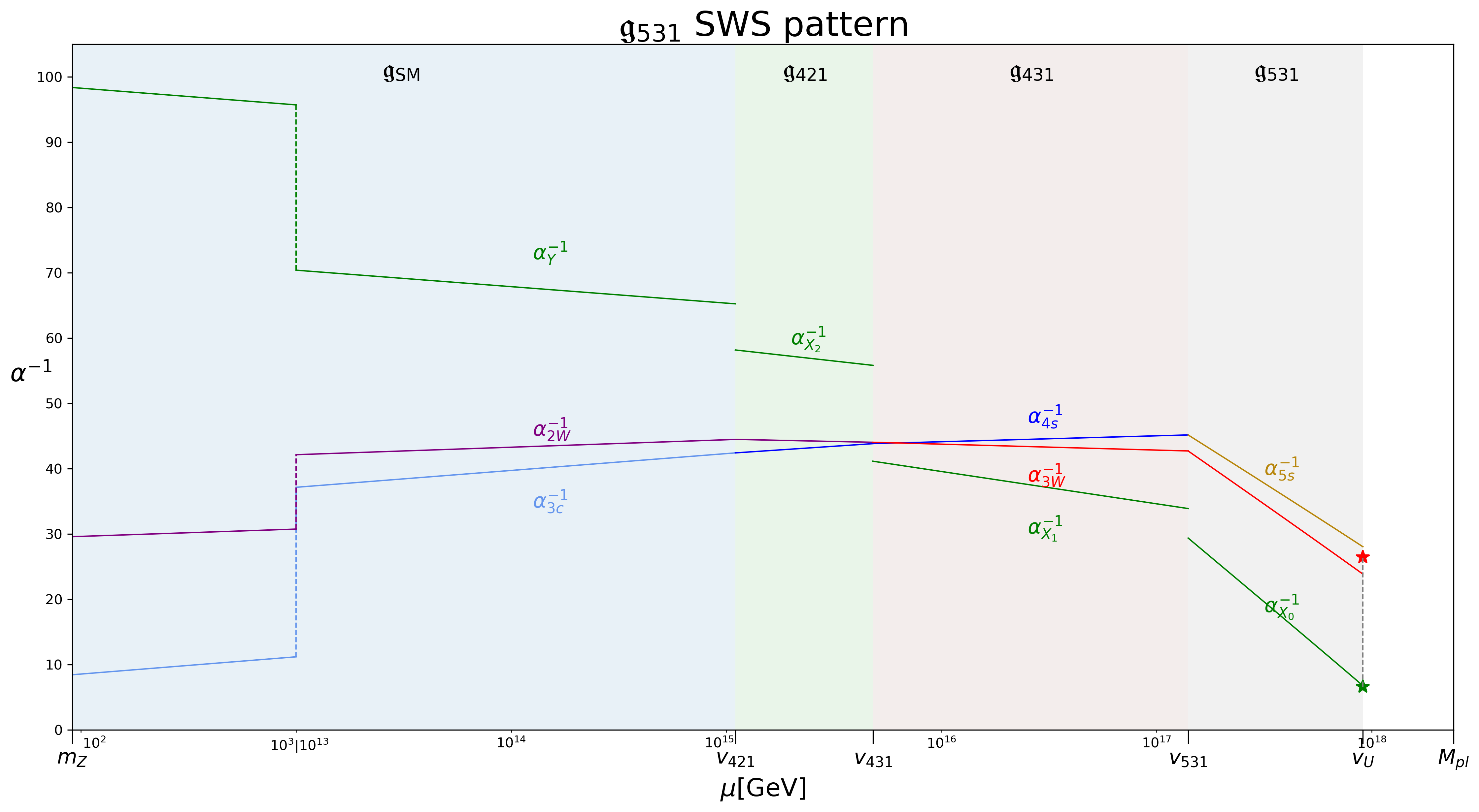
Figure 2: The two-loop RGEs of the ${\mathfrak{s}\mathfrak{u}}(8)$ setup according to the SWS symmetry breaking pattern. The RG evolutions within $10^{3}\,{\rm GeV}\lesssim\mu\lesssim 10^{13}\,{\rm GeV}$ are zoomed out in order to highlight the behaviors in three intermediate symmetry breaking scales given by the benchmark point in Eq. (151).

With the one- and two-loop $\beta$ coefficients defined in Eqs. (3.3), (3.3), (3.3), and (2.3), we plot the RGEs of the ${\mathfrak{s}\mathfrak{u}}(8)$ setup along the SWS symmetry breaking pattern in Fig. 2. The discontinuities of the ${\mathfrak{u}}(1)$ gauge couplings at three intermediate scales follow from their definitions in Eqs. (41), (44), (45), respectively. The benchmark point in Fig. 2 is marked by $\star$ and reads

$$c_{\rm HSW}\approx-0.81\,,\penalty 10000\ v_{U}\approx 9.09\times 10^{17}\,{\rm GeV}\,,$$

$$\alpha_{5c}^{-1}(v_{U})\approx 28.05\,,\penalty 10000\ \alpha_{3W}^{-1}(v_{U})\approx 23.86\,,\penalty 10000\ \alpha_{X_{0}}^{-1}(v_{U})\approx 6.77\,.$$ (46)

4 The WSS symmetry breaking pattern

4.1 Decompositions of the ${\mathfrak{s}\mathfrak{u}}$(8) fermions

${\mathfrak{s}\mathfrak{u}}(8)$	$\mathfrak{g}_{531}$	$\mathfrak{g}_{521}$	$\mathfrak{g}_{421}$	$\mathfrak{g}_{\rm SM}$
$\mathbf{\overline{8_{F}}}^{\Omega}$	$(\mathbf{\overline{5}}\,,\mathbf{1}\,,+\frac{1}{5})_{\mathbf{F}}^{\Omega}$	$(\mathbf{\overline{5}}\,,\mathbf{1}\,,+\frac{1}{5})_{\mathbf{F}}^{\Omega}$	$(\mathbf{\overline{4}}\,,\mathbf{1}\,,+\frac{1}{4})_{\mathbf{F}}^{\Omega}$	$(\mathbf{\overline{3}}\,,\mathbf{1}\,,+\frac{1}{3})_{\mathbf{F}}^{\Omega}\penalty 10000\ :\penalty 10000\ {\mathcal{D}_{R}^{\Omega}}^{c}$
				$(\mathbf{1}\,,\mathbf{1}\,,0)_{\mathbf{F}}^{\Omega}\penalty 10000\ :\penalty 10000\ \check{\mathcal{N}}_{L}^{\Omega}$
			$(\mathbf{1}\,,\mathbf{1}\,,0)_{\mathbf{F}}^{\Omega^{\prime}}$	$(\mathbf{1}\,,\mathbf{1}\,,0)_{\mathbf{F}}^{\Omega^{\prime}}\penalty 10000\ :\penalty 10000\ \check{\mathcal{N}}_{L}^{\Omega^{\prime}}$
	$(\mathbf{1}\,,\mathbf{\overline{3}}\,,-\frac{1}{3})_{\mathbf{F}}^{\Omega}$	$(\mathbf{1}\,,\mathbf{\overline{2}}\,,-\frac{1}{2})_{\mathbf{F}}^{\Omega}$	$(\mathbf{1}\,,\mathbf{\overline{2}}\,,-\frac{1}{2})_{\mathbf{F}}^{\Omega}$	$(\mathbf{1}\,,\mathbf{\overline{2}}\,,-\frac{1}{2})_{\mathbf{F}}^{\Omega}\penalty 10000\ :\penalty 10000\ \mathcal{L}_{L}^{\Omega}=(\mathcal{E}_{L}^{\Omega}\,,-\mathcal{N}_{L}^{\Omega})^{T}$
		$(\mathbf{1}\,,\mathbf{1}\,,0)_{\mathbf{F}}^{\Omega^{\prime\prime}}$	$(\mathbf{1}\,,\mathbf{1}\,,0)_{\mathbf{F}}^{\Omega^{\prime\prime}}$	$(\mathbf{1}\,,\mathbf{1}\,,0)_{\mathbf{F}}^{\Omega^{\prime\prime}}\penalty 10000\ :\penalty 10000\ \check{\mathcal{N}}_{L}^{\Omega^{\prime\prime}}$

Table 8: The ${\mathfrak{s}\mathfrak{u}}(8)$ fermion representation of $\mathbf{\overline{8_{F}}}^{\Omega}$ under the $\mathfrak{g}_{531}\,,\mathfrak{g}_{521}\,,\mathfrak{g}_{421}\,,\mathfrak{g}_{\rm SM}$ subalgebras.

${\mathfrak{s}\mathfrak{u}}(8)$	$\mathfrak{g}_{531}$	$\mathfrak{g}_{521}$	$\mathfrak{g}_{421}$	$\mathfrak{g}_{\rm SM}$
$\mathbf{28_{F}}$	$(\mathbf{1}\,,\mathbf{\overline{3}}\,,+\frac{2}{3})_{\mathbf{F}}$	$(\mathbf{1}\,,\mathbf{\overline{2}}\,,+\frac{1}{2})_{\mathbf{F}}$	$(\mathbf{1}\,,\mathbf{\overline{2}}\,,+\frac{1}{2})_{\mathbf{F}}$	$(\mathbf{1}\,,\mathbf{\overline{2}}\,,+\frac{1}{2})_{\mathbf{F}}\penalty 10000\ :\penalty 10000\ ({\mathfrak{n}_{R}}^{c}\,,-{\mathfrak{e}_{R}}^{c})^{T}$
		$(\mathbf{1}\,,\mathbf{1}\,,+1)_{\mathbf{F}}$	$(\mathbf{1}\,,\mathbf{1}\,,+1)_{\mathbf{F}}$	$\underline{(\mathbf{1}\,,\mathbf{1}\,,+1)_{\mathbf{F}}\penalty 10000\ :\penalty 10000\ {\tau_{R}}^{c}}$
	$(\mathbf{5}\,,\mathbf{3}\,,+\frac{2}{15})_{\mathbf{F}}$	$(\mathbf{5}\,,\mathbf{1}\,,-\frac{1}{5})_{\mathbf{F}}$	$(\mathbf{4}\,,\mathbf{1}\,,-\frac{1}{4})_{\mathbf{F}}$	$(\mathbf{3}\,,\mathbf{1}\,,-\frac{1}{3})_{\mathbf{F}}\penalty 10000\ :\penalty 10000\ \mathfrak{D}_{L}$
				$(\mathbf{1}\,,\mathbf{1}\,,0)_{\mathbf{F}}\penalty 10000\ :\penalty 10000\ \check{\mathfrak{n}}_{R}^{c}$
			$(\mathbf{1}\,,\mathbf{1}\,,0)_{\mathbf{F}}^{\prime}$	$(\mathbf{1}\,,\mathbf{1}\,,0)_{\mathbf{F}}^{\prime}\penalty 10000\ :\penalty 10000\ \check{\mathfrak{n}}_{R}^{\prime\,c}$
		$(\mathbf{5}\,,\mathbf{2}\,,+\frac{3}{10})_{\mathbf{F}}$	$(\mathbf{1}\,,\mathbf{2}\,,+\frac{1}{2})_{\mathbf{F}}^{\prime}$	$(\mathbf{1}\,,\mathbf{2}\,,+\frac{1}{2})_{\mathbf{F}}^{\prime}\penalty 10000\ :\penalty 10000\ ({\mathfrak{e}_{R}^{\prime}}^{c}\,,{\mathfrak{n}_{R}^{\prime}}^{c})^{T}$
			$(\mathbf{4}\,,\mathbf{2}\,,+\frac{1}{4})_{\mathbf{F}}$	$(\mathbf{1}\,,\mathbf{2}\,,+\frac{1}{2})_{\mathbf{F}}^{\prime\prime}\penalty 10000\ :\penalty 10000\ ({\mathfrak{e}_{R}^{\prime\prime}}^{c}\,,{\mathfrak{n}_{R}^{\prime\prime}}^{c})^{T}$
				$\underline{(\mathbf{3}\,,\mathbf{2}\,,+\frac{1}{6})_{\mathbf{F}}\penalty 10000\ :\penalty 10000\ (t_{L}\,,b_{L})^{T}}$
	$(\mathbf{10}\,,\mathbf{1}\,,-\frac{2}{5})_{\mathbf{F}}$	$(\mathbf{10}\,,\mathbf{1}\,,-\frac{2}{5})_{\mathbf{F}}$	$(\mathbf{4}\,,\mathbf{1}\,,-\frac{1}{4})_{\mathbf{F}}^{\prime}$	$(\mathbf{3}\,,\mathbf{1}\,,-\frac{1}{3})_{\mathbf{F}}^{\prime}\penalty 10000\ :\penalty 10000\ \mathfrak{D}_{L}^{\prime}$
				$(\mathbf{1}\,,\mathbf{1}\,,0)_{\mathbf{F}}^{\prime\prime}\penalty 10000\ :\penalty 10000\ \check{\mathfrak{n}}_{R}^{\prime\prime\,c}$
			$(\mathbf{6}\,,\mathbf{1}\,,-\frac{1}{2})_{\mathbf{F}}$	$(\mathbf{3}\,,\mathbf{1}\,,-\frac{1}{3})_{\mathbf{F}}^{\prime\prime}\penalty 10000\ :\penalty 10000\ \mathfrak{D}_{L}^{\prime\prime}$
				$\underline{(\mathbf{\overline{3}}\,,\mathbf{1}\,,-\frac{2}{3})_{\mathbf{F}}\penalty 10000\ :\penalty 10000\ {t_{R}}^{c}}$

Table 9: The ${\mathfrak{s}\mathfrak{u}}(8)$ fermion representation of $\mathbf{28_{F}}$ under the $\mathfrak{g}_{531}\,,\mathfrak{g}_{521}\,,\mathfrak{g}_{421}\,,\mathfrak{g}_{\rm SM}$ subalgebras. All IRs for SM fermions are marked with underlines.

${\mathfrak{s}\mathfrak{u}}(8)$	$\mathfrak{g}_{531}$	$\mathfrak{g}_{521}$	$\mathfrak{g}_{421}$	$\mathfrak{g}_{\rm SM}$
$\mathbf{56_{F}}$	$(\mathbf{1}\,,\mathbf{1}\,,+1)_{\mathbf{F}}^{\prime}$	$(\mathbf{1}\,,\mathbf{1}\,,+1)_{\mathbf{F}}^{\prime}$	$(\mathbf{1}\,,\mathbf{1}\,,+1)_{\mathbf{F}}^{\prime}$	$\underline{(\mathbf{1}\,,\mathbf{1}\,,+1)_{\mathbf{F}}^{\prime}\penalty 10000\ :\penalty 10000\ {\mu_{R}}^{c}}$
	$(\mathbf{5}\,,\mathbf{\overline{3}}\,,+\frac{7}{15})_{\mathbf{F}}$	$(\mathbf{5}\,,\mathbf{1}\,,+\frac{4}{5})_{\mathbf{F}}$	$(\mathbf{1}\,,\mathbf{1}\,,+1)_{\mathbf{F}}^{\prime\prime}$	$\underline{(\mathbf{1}\,,\mathbf{1}\,,+1)_{\mathbf{F}}^{\prime\prime}\penalty 10000\ :\penalty 10000\ {e_{R}}^{c}}$
			$(\mathbf{4}\,,\mathbf{1}\,,+\frac{3}{4})_{\mathbf{F}}$	$(\mathbf{1}\,,\mathbf{1}\,,+1)_{\mathbf{F}}^{\prime\prime\prime}\penalty 10000\ :\penalty 10000\ {\mathfrak{E}_{R}}^{c}$
				$(\mathbf{3}\,,\mathbf{1}\,,+\frac{2}{3})_{\mathbf{F}}\penalty 10000\ :\penalty 10000\ \mathfrak{U}_{L}$
		$(\mathbf{5}\,,\mathbf{\overline{2}}\,,+\frac{3}{10})_{\mathbf{F}}$	$(\mathbf{1}\,,\mathbf{\overline{2}}\,,+\frac{1}{2})_{\mathbf{F}}^{\prime\prime\prime}$	$(\mathbf{1}\,,\mathbf{\overline{2}}\,,+\frac{1}{2})_{\mathbf{F}}^{\prime\prime\prime}\penalty 10000\ :\penalty 10000\ ({\mathfrak{n}_{R}^{\prime\prime\prime}}^{c}\,,-{\mathfrak{e}_{R}^{\prime\prime\prime}}^{c})^{T}$
			$(\mathbf{4}\,,\mathbf{\overline{2}}\,,+\frac{1}{4})_{\mathbf{F}}$	$(\mathbf{1}\,,\mathbf{\overline{2}}\,,+\frac{1}{2})_{\mathbf{F}}^{\prime\prime\prime\prime}\penalty 10000\ :\penalty 10000\ ({\mathfrak{n}_{R}^{\prime\prime\prime\prime}}^{c}\,,-{\mathfrak{e}_{R}^{\prime\prime\prime\prime}}^{c})^{T}$
				$(\mathbf{3}\,,\mathbf{\overline{2}}\,,+\frac{1}{6})_{\mathbf{F}}\penalty 10000\ :\penalty 10000\ (\mathfrak{d}_{L}\,,-\mathfrak{u}_{L})^{T}$
	$(\mathbf{\overline{10}}\,,\mathbf{1}\,,-\frac{3}{5})_{\mathbf{F}}$	$(\mathbf{\overline{10}}\,,\mathbf{1}\,,-\frac{3}{5})_{\mathbf{F}}$	$(\mathbf{\overline{4}}\,,\mathbf{1}\,,-\frac{3}{4})_{\mathbf{F}}$	$(\mathbf{1}\,,\mathbf{1}\,,-1)_{\mathbf{F}}\penalty 10000\ :\penalty 10000\ \mathfrak{E}_{L}$
				$(\mathbf{\overline{3}}\,,\mathbf{1}\,,-\frac{2}{3})_{\mathbf{F}}^{\prime}\penalty 10000\ :\penalty 10000\ {\mathfrak{U}_{R}}^{c}$
			$(\mathbf{6}\,,\mathbf{1}\,,-\frac{1}{2})_{\mathbf{F}}^{\prime}$	$(\mathbf{3}\,,\mathbf{1}\,,-\frac{1}{3})_{\mathbf{F}}^{\prime\prime\prime}\penalty 10000\ :\penalty 10000\ \mathfrak{D}_{L}^{\prime\prime\prime}$
				$\underline{(\mathbf{\overline{3}}\,,\mathbf{1}\,,-\frac{2}{3})_{\mathbf{F}}^{\prime\prime}\penalty 10000\ :\penalty 10000\ {u_{R}}^{c}}$
	$(\mathbf{10}\,,\mathbf{3}\,,-\frac{1}{15})_{\mathbf{F}}$	$(\mathbf{10}\,,\mathbf{1}\,,-\frac{2}{5})_{\mathbf{F}}^{\prime}$	$(\mathbf{4}\,,\mathbf{1}\,,-\frac{1}{4})_{\mathbf{F}}^{\prime\prime}$	$(\mathbf{3}\,,\mathbf{1}\,,-\frac{1}{3})_{\mathbf{F}}^{\prime\prime\prime\prime}\penalty 10000\ :\penalty 10000\ \mathfrak{D}_{L}^{\prime\prime\prime\prime}$
				$(\mathbf{1}\,,\mathbf{1}\,,0)_{\mathbf{F}}^{\prime\prime\prime}\penalty 10000\ :\penalty 10000\ {\check{\mathfrak{n}}_{R}}^{\prime\prime\prime\,c}$
			$(\mathbf{6}\,,\mathbf{1}\,,-\frac{1}{2})_{\mathbf{F}}^{\prime\prime}$	$(\mathbf{3}\,,\mathbf{1}\,,-\frac{1}{3})_{\mathbf{F}}^{\prime\prime\prime\prime\prime}\penalty 10000\ :\penalty 10000\ \mathfrak{D}_{L}^{\prime\prime\prime\prime\prime}$
				$\underline{(\mathbf{\overline{3}}\,,\mathbf{1}\,,-\frac{2}{3})_{\mathbf{F}}^{\prime\prime\prime}\penalty 10000\ :\penalty 10000\ {c_{R}}^{c}}$
		$(\mathbf{10}\,,\mathbf{2}\,,+\frac{1}{10})_{\mathbf{F}}$	$(\mathbf{4}\,,\mathbf{2}\,,+\frac{1}{4})_{\mathbf{F}}^{\prime}$	$\underline{(\mathbf{3}\,,\mathbf{2}\,,+\frac{1}{6})_{\mathbf{F}}^{\prime}\penalty 10000\ :\penalty 10000\ (u_{L}\,,d_{L})^{T}}$
				$(\mathbf{1}\,,\mathbf{2}\,,+\frac{1}{2})_{\mathbf{F}}^{\prime\prime\prime\prime\prime}\penalty 10000\ :\penalty 10000\ ({\mathfrak{e}_{R}^{\prime\prime\prime\prime\prime}}^{c}\,,{\mathfrak{n}_{R}^{\prime\prime\prime\prime\prime}}^{c})^{T}$
			$(\mathbf{6}\,,\mathbf{2}\,,0)_{\mathbf{F}}$	$\underline{(\mathbf{3}\,,\mathbf{2}\,,+\frac{1}{6})_{\mathbf{F}}^{\prime\prime}\penalty 10000\ :\penalty 10000\ (c_{L}\,,s_{L})^{T}}$
				$(\mathbf{\overline{3}}\,,\mathbf{2}\,,-\frac{1}{6})_{\mathbf{F}}\penalty 10000\ :\penalty 10000\ ({\mathfrak{d}_{R}}^{c}\,,{\mathfrak{u}_{R}}^{c})^{T}$

Table 10: The ${\mathfrak{s}\mathfrak{u}}(8)$ fermion representation of $\mathbf{56_{F}}$ under the $\mathfrak{g}_{531}\,,\mathfrak{g}_{521}\,,\mathfrak{g}_{421}\,,\mathfrak{g}_{\rm SM}$ subalgebras. All IRs for SM fermions are marked with underlines.

By following the WSS symmetry breaking pattern in Eq. (13c), we tabulate the fermion representations at various stages in Tables 8, 9, and 10. Along this pattern, the global $\widetilde{{\rm U}}(1)_{T}$ symmetry evolves to the global $\widetilde{{\rm U}}(1)_{B-L}$ at the EW scale according to the following sequence:

$$\mathfrak{g}_{531}\penalty 10000\ :\penalty 10000\ \mathcal{T}^{\prime}\equiv\mathcal{T}+3t\mathcal{X}_{0}\,,\quad\mathfrak{g}_{521}\penalty 10000\ :\penalty 10000\ \mathcal{T}^{\prime\prime}\equiv\mathcal{T}^{\prime}-8t\mathcal{X}_{1}\,,$$

$$\mathfrak{g}_{421}\penalty 10000\ :\penalty 10000\ \mathcal{T}^{\prime\prime\prime}\equiv\mathcal{T}^{\prime\prime}\,,\quad\mathfrak{g}_{\rm SM}\penalty 10000\ :\penalty 10000\ \mathcal{B}-\mathcal{L}\equiv\mathcal{T}^{\prime\prime\prime}+8t\mathcal{Y}\,.$$ (47)

4.2 Decompositions of the ${\mathfrak{s}\mathfrak{u}}$(8) Higgs fields

We decompose the Higgs fields in Eq. (6) into components that can be responsible for the sequential symmetry breaking stages in Eq. (13c). For Higgs fields of $\mathbf{\overline{8_{H}}}_{\,,\omega}$, they read

$$\mathbf{\overline{8_{H}}}_{\,,\omega} \supset \langle(\mathbf{1}\,,\mathbf{\overline{3}}\,,-\frac{1}{3})_{\mathbf{H}\,,\omega}\rangle\oplus\underline{(\mathbf{\overline{5}}\,,\mathbf{1}\,,+\frac{1}{5})_{\mathbf{H}\,,\omega}}$$ (48)

$$\supset \underline{(\mathbf{1}\,,\mathbf{\overline{2}}\,,-\frac{1}{2})_{\mathbf{H}\,,\omega}}\oplus\langle(\mathbf{\overline{5}}\,,\mathbf{1}\,,+\frac{1}{5})_{\mathbf{H}\,,\omega}\rangle$$

$$\supset \underline{(\mathbf{1}\,,\mathbf{\overline{2}}\,,-\frac{1}{2})_{\mathbf{H}\,,\omega}}\oplus\langle(\mathbf{\overline{4}}\,,\mathbf{1}\,,+\frac{1}{4})_{\mathbf{H}\,,\omega}\rangle\,.$$

For Higgs fields of $\mathbf{\overline{28_{H}}}_{\,,\dot{\omega}}$, they read

$$\mathbf{\overline{28_{H}}}_{\,,\dot{\omega}} \supset \underline{(\mathbf{1}\,,\mathbf{3}\,,-\frac{2}{3})_{\mathbf{H}\,,\dot{\omega}}}\oplus\underline{(\mathbf{\overline{5}}\,,\mathbf{\overline{3}}\,,-\frac{2}{15})_{\mathbf{H}\,,\dot{\omega}}}\oplus\underline{(\mathbf{\overline{10}}\,,\mathbf{1}\,,+\frac{2}{5})_{\mathbf{H}\,,\dot{\omega}}}$$ (49)

$$\supset \underline{(\mathbf{1}\,,\mathbf{2}\,,-\frac{1}{2})_{\mathbf{H}\,,\dot{\omega}}}\oplus\Big[\underline{(\mathbf{\overline{5}}\,,\mathbf{\overline{2}}\,,-\frac{3}{10})_{\mathbf{H}\,,\dot{\omega}}}\oplus\langle(\mathbf{\overline{5}}\,,\mathbf{1}\,,+\frac{1}{5})_{\mathbf{H}\,,\dot{\omega}}\rangle\Big]\oplus\underline{(\mathbf{\overline{10}}\,,\mathbf{1}\,,+\frac{2}{5})_{\mathbf{H}\,,\dot{\omega}}}$$

$$\supset \underline{(\mathbf{1}\,,\mathbf{2}\,,-\frac{1}{2})_{\mathbf{H}\,,\dot{\omega}}}\oplus\Big[\underline{(\mathbf{1}\,,\mathbf{\overline{2}}\,,-\frac{1}{2})_{\mathbf{H}\,,\dot{\omega}}}\oplus\underline{(\mathbf{\overline{4}}\,,\mathbf{\overline{2}}\,,-\frac{1}{4})_{\mathbf{H}\,,\dot{\omega}}}\oplus\langle(\mathbf{\overline{4}}\,,\mathbf{1}\,,+\frac{1}{4})_{\mathbf{H}\,,\dot{\omega}}\rangle\Big]$$

$$\oplus \langle(\mathbf{\overline{4}}\,,\mathbf{1}\,,+\frac{1}{4})_{\mathbf{H}\,,\dot{\omega}}^{\prime}\rangle\,.$$

For Higgs field of $\mathbf{70_{H}}$, it reads

$$\mathbf{70_{H}} \supset (\mathbf{5}\,,\mathbf{1}\,,+\frac{4}{5})_{\mathbf{H}}\oplus(\mathbf{\overline{5}}\,,\mathbf{1}\,,-\frac{4}{5})_{\mathbf{H}}\oplus\underline{(\mathbf{10}\,,\mathbf{\overline{3}}\,,+\frac{4}{15})_{\mathbf{H}}}\oplus(\mathbf{\overline{10}}\,,\mathbf{3}\,,-\frac{4}{15})_{\mathbf{H}}$$ (50)

$$\supset \underline{(\mathbf{10}\,,\mathbf{\overline{2}}\,,+\frac{1}{10})_{\mathbf{H}}}\supset\underline{(\mathbf{4}\,,\mathbf{\overline{2}}\,,+\frac{1}{4})_{\mathbf{H}}}\supset\langle(\mathbf{1}\,,\mathbf{\overline{2}}\,,+\frac{1}{2})_{\mathbf{H}}\rangle\,.$$

4.3 RGEs of the WSS symmetry breaking pattern

Between the $v_{531}\leq\mu\leq v_{U}$, almost all massless Higgs fields are summarized as follows:

$$(\mathbf{\overline{5}}\,,\mathbf{1}\,,+\frac{1}{5})_{\mathbf{H}\,,\omega}\oplus(\mathbf{1}\,,\mathbf{\overline{3}}\,,-\frac{1}{3})_{\mathbf{H}\,,\omega}\subset\mathbf{\overline{8_{H}}}_{,\omega}\,,$$

$$(\mathbf{1}\,,\mathbf{3}\,,-\frac{2}{3})_{\mathbf{H}\,,\dot{\omega}}\oplus(\mathbf{\overline{5}}\,,\mathbf{\overline{3}}\,,-\frac{2}{15})_{\mathbf{H}\,,\dot{\omega}}\oplus(\mathbf{\overline{10}}\,,\mathbf{1}\,,+\frac{2}{5})_{\mathbf{H}\,,\dot{\omega}}\subset\mathbf{\overline{28_{H}}}_{,\dot{\omega}}\,,$$

$$(\mathbf{5}\,,\mathbf{1}\,,+\frac{4}{5})_{\mathbf{H}}\oplus(\mathbf{\overline{5}}\,,\mathbf{1}\,,-\frac{4}{5})_{\mathbf{H}}\oplus(\mathbf{10}\,,\mathbf{\overline{3}}\,,+\frac{4}{15})_{\mathbf{H}}\oplus(\mathbf{\overline{10}}\,,\mathbf{3}\,,-\frac{4}{15})_{\mathbf{H}}\subset\mathbf{70_{H}}\,,$$

$$(\mathbf{\overline{5}}\,,\mathbf{1}\,,-\frac{4}{5})_{\mathbf{H}}\oplus(\mathbf{5}\,,\mathbf{1}\,,+\frac{4}{5})_{\mathbf{H}}\oplus(\mathbf{\overline{10}}\,,\mathbf{3}\,,-\frac{4}{15})_{\mathbf{H}}\oplus(\mathbf{10}\,,\mathbf{\overline{3}}\,,+\frac{4}{15})_{\mathbf{H}}\subset\mathbf{\overline{70_{H}}}\,,$$

$$(\mathbf{5}\,,\mathbf{1}\,,-\frac{1}{5})_{\mathbf{H}}^{\omega}\oplus(\mathbf{1}\,,\mathbf{3}\,,+\frac{1}{3})_{\mathbf{H}}^{\omega}\subset\mathbf{8_{H}}^{\omega}\,,$$

$$(\mathbf{1}\,,\mathbf{\overline{3}}\,,+\frac{2}{3})_{\mathbf{H}}^{\dot{\omega}}\oplus(\mathbf{5}\,,\mathbf{3}\,,+\frac{2}{15})_{\mathbf{H}}^{\dot{\omega}}\oplus(\mathbf{10}\,,\mathbf{1}\,,-\frac{2}{5})_{\mathbf{H}}^{\dot{\omega}}\subset\mathbf{28_{H}}^{\dot{\omega}}\,.$$ (51)

All fermionic components of $\mathbf{\overline{8_{F}}}^{\Omega}\oplus\mathbf{28_{F}}\oplus\mathbf{56_{F}}$ remain massless after the decomposition into the $\mathfrak{g}_{531}$ IRs. Consequently, we have the $\mathfrak{g}_{531}$ $\beta$ coefficients of

$$(b^{(1)}_{{\mathfrak{s}\mathfrak{u}}(5)_{s}}\,,b^{(1)}_{{\mathfrak{s}\mathfrak{u}}(3)_{W}}\,,b^{(1)}_{{\mathfrak{u}}(1)_{X_{0}}})=(+54\,,+60\,,+\frac{368}{5})\,,$$

$$b^{(2)}_{\mathfrak{g}_{531}}=\begin{pmatrix}6984/5&216&672/25\\ 648&728&352/15\\ 16128/25&2816/15&98816/1125\end{pmatrix}\,.$$ (52)

Between the $v_{521}\leq\mu\leq v_{531}$, the massless Higgs fields are

$$(\mathbf{\overline{5}}\,,\mathbf{1}\,,+\frac{1}{5})_{\mathbf{H}\,,3,\rm V,\rm VI}\oplus(\mathbf{1}\,,\mathbf{\overline{2}}\,,-\frac{1}{2})_{\mathbf{H}\,,3,\rm V,\rm VI}\subset...\subset\mathbf{\overline{8_{H}}}_{\,,3,\rm V,\rm VI}\,,$$ (53)

$$(\mathbf{\overline{10}}\,,\mathbf{1}\,,+\frac{2}{5})_{\mathbf{H}\,,\dot{\omega}}\oplus\Big[(\mathbf{1}\,,\mathbf{2}\,,-\frac{1}{2})_{\mathbf{H}\,,\dot{\omega}}\oplus(\mathbf{1}\,,\mathbf{1}\,,-1)_{\mathbf{H}\,,\dot{\omega}}\Big]$$

$$\oplus \Big[(\mathbf{\overline{5}}\,,\mathbf{1}\,,+\frac{1}{5})_{\mathbf{H}\,,\dot{\omega}}\oplus(\mathbf{\overline{5}}\,,\mathbf{\overline{2}}\,,-\frac{3}{10})_{\mathbf{H}\,,\dot{\omega}}\Big]\subset...\subset\mathbf{\overline{28_{H}}}_{\,,\dot{\omega}}\,,\quad\dot{\omega}=(\dot{1},\dot{2},\dot{\rm VII},\dot{\rm VIII},\dot{\rm IX})\,,$$

$$(\mathbf{10}\,,\mathbf{1}\,,-\frac{2}{5})_{\mathbf{H}}^{\dot{\rm\kappa}}\oplus\Big[(\mathbf{1}\,,\mathbf{\overline{2}}\,,+\frac{1}{2})_{\mathbf{H}}^{\dot{\rm\kappa}}\oplus(\mathbf{1}\,,\mathbf{1}\,,+1)_{\mathbf{H}}^{\dot{\rm\kappa}}\Big]$$

$$\oplus \Big[(\mathbf{5}\,,\mathbf{1}\,,-\frac{1}{5})_{\mathbf{H}}^{\dot{\rm\kappa}}\oplus(\mathbf{5}\,,\mathbf{2}\,,+\frac{3}{10})_{\mathbf{H}}^{\dot{\rm\kappa}}\Big]\subset...\subset\mathbf{28_{H}}^{\dot{\rm\kappa}}\,,\quad\dot{\kappa}=(\dot{\rm VII},\dot{\rm IX})\,,$$

$$(\mathbf{10}\,,\mathbf{\overline{2}}\,,+\frac{1}{10})_{\mathbf{H}}\subset...\subset\mathbf{70_{H}}\,.$$

All ${\mathfrak{s}\mathfrak{u}}$(8) fermions in Eq. (155) remain massless after the decomposition into the $\mathfrak{g}_{521}$ IRs. Consequently, we have the $\mathfrak{g}_{521}$ $\beta$ coefficients of

$$(b^{(1)}_{{\mathfrak{s}\mathfrak{u}}(5)_{s}}\,,b^{(1)}_{{\mathfrak{s}\mathfrak{u}}(2)_{W}}\,,b^{(1)}_{{\mathfrak{u}}(1)_{X_{1}}})=(-\frac{1}{2}\,,+\frac{67}{6}\,,+\frac{709}{30})\,,$$

$$b^{(2)}_{\mathfrak{g}_{521}}=\begin{pmatrix}2149/5&75/2&679/50\\ 300&1129/6&29/2\\ 8148/25&87/2&14233/250\end{pmatrix}\,.$$ (54)

The ${\mathfrak{s}\mathfrak{u}}(3)_{W}\oplus{\mathfrak{u}}(1)_{X_{0}}$ gauge couplings match with the ${\mathfrak{s}\mathfrak{u}}(2)_{W}\oplus{\mathfrak{u}}(1)_{X_{1}}$ gauge couplings as follows:

$$\alpha_{3W}^{-1}(v_{531})=\alpha_{2W}^{-1}(v_{531})\,,\penalty 10000\ \alpha_{X_{1}}^{-1}(v_{531})=\frac{1}{3}\alpha_{3W}^{-1}(v_{531})+\alpha_{X_{0}}^{-1}(v_{531})\,.$$ (55)

Between the $v_{421}\leq\mu\leq v_{521}$, the massless Higgs fields are

$$(\mathbf{\overline{4}}\,,\mathbf{1}\,,+\frac{1}{4})_{\mathbf{H}\,,3,\rm VI}\oplus(\mathbf{1}\,,\mathbf{\overline{2}}\,,-\frac{1}{2})_{\mathbf{H}\,,3,\rm VI}\subset...\subset\mathbf{\overline{8_{H}}}_{,3,\rm VI}\,,$$ (56)

$$\Big[(\mathbf{\overline{4}}\,,\mathbf{1}\,,+\frac{1}{4})_{\mathbf{H}\,,\dot{\omega}}^{\prime}\oplus(\mathbf{6}\,,\mathbf{1}\,,+\frac{1}{2})_{\mathbf{H}\,,\dot{\omega}}\Big]\oplus\Big[(\mathbf{1}\,,\mathbf{2}\,,-\frac{1}{2})_{\mathbf{H}\,,\dot{\omega}}\oplus(\mathbf{1}\,,\mathbf{1}\,,-1)_{\mathbf{H}\,,\dot{\omega}}\Big]$$

$$\oplus \Big[(\mathbf{\overline{4}}\,,\mathbf{1}\,,+\frac{1}{4})_{\mathbf{H}\,,\dot{\omega}}\oplus(\mathbf{1}\,,\mathbf{\overline{2}}\,,-\frac{1}{2})_{\mathbf{H}\,,\dot{\omega}}\oplus(\mathbf{\overline{4}}\,,\mathbf{\overline{2}}\,,-\frac{1}{4})_{\mathbf{H}\,,\dot{\omega}}\Big]\subset...\subset\mathbf{\overline{28_{H}}}_{\,,\dot{\omega}}\,,\quad\dot{\omega}=(\dot{2},\dot{\rm VIII},\dot{\rm IX})\,,$$

$$\Big[(\mathbf{4}\,,\mathbf{1}\,,-\frac{1}{4})_{\mathbf{H}}^{\dot{\rm IX}^{\prime}}\oplus(\mathbf{6}\,,\mathbf{1}\,,-\frac{1}{2})_{\mathbf{H}}^{\dot{\rm IX}}\Big]\oplus\Big[(\mathbf{1}\,,\mathbf{\overline{2}}\,,+\frac{1}{2})_{\mathbf{H}}^{\dot{\rm IX}}\oplus(\mathbf{1}\,,\mathbf{1}\,,+1)_{\mathbf{H}}^{\dot{\rm IX}}\Big]$$

$$\oplus \Big[(\mathbf{4}\,,\mathbf{1}\,,-\frac{1}{4})_{\mathbf{H}}^{\dot{\rm IX}}\oplus(\mathbf{1}\,,\mathbf{2}\,,+\frac{1}{2})_{\mathbf{H}}^{\dot{\rm IX}}\oplus(\mathbf{4}\,,\mathbf{2}\,,+\frac{1}{4})_{\mathbf{H}}^{\dot{\rm IX}}\Big]\subset...\subset\mathbf{28_{H}}^{\dot{\rm IX}}\,,$$

$$(\mathbf{4}\,,\mathbf{\overline{2}}\,,+\frac{1}{4})_{\mathbf{H}}\subset...\subset\mathbf{70_{H}}\,.$$

All ${\mathfrak{s}\mathfrak{u}}$(8) fermions in Eq. (159) remain massless after the decomposition into the $\mathfrak{g}_{421}$ IRs. Consequently, we have the $\mathfrak{g}_{421}$ $\beta$ coefficients of

$$(b^{(1)}_{{\mathfrak{s}\mathfrak{u}}(4)_{s}}\,,b^{(1)}_{{\mathfrak{s}\mathfrak{u}}(2)_{W}}\,,b^{(1)}_{{\mathfrak{u}}(1)_{X_{2}}})=(-\frac{8}{3}\,,+\frac{17}{3}\,,+\frac{47}{3})\,,$$

$$b^{(2)}_{\mathfrak{g}_{421}}=\begin{pmatrix}991/6&45/2&35/4\\ 225/2&353/3&39/4\\ 525/4&117/4&307/8\end{pmatrix}\,.$$ (57)

The ${\mathfrak{s}\mathfrak{u}}(5)_{s}\oplus{\mathfrak{u}}(1)_{X_{1}}$ gauge couplings match with the ${\mathfrak{s}\mathfrak{u}}(4)_{s}\oplus{\mathfrak{u}}(1)_{X_{2}}$ gauge couplings as follows:

$$\alpha_{5s}^{-1}(v_{521})=\alpha_{4s}^{-1}(v_{521})\,,\penalty 10000\ \alpha_{X_{2}}^{-1}(v_{521})=\frac{1}{10}\alpha_{5s}^{-1}(v_{521})+\alpha_{X_{1}}^{-1}(v_{521})\,.$$ (58)

Between the $v_{\rm EW}\leq\mu\leq v_{421}$, we have the same $\mathfrak{g}_{\rm SM}$ $\beta$ coefficients as Eq. (2.3). The ${\mathfrak{s}\mathfrak{u}}(4)_{s}\oplus{\mathfrak{u}}(1)_{X_{2}}$ gauge couplings match with the ${\mathfrak{s}\mathfrak{u}}(3)_{c}\oplus{\mathfrak{u}}(1)_{\rm Y}$ gauge couplings as follows:

$$\alpha_{4s}^{-1}(v_{421})=\alpha_{3c}^{-1}(v_{421})\,,\penalty 10000\ \alpha_{\rm Y}^{-1}(v_{421})=\frac{1}{6}\alpha_{4s}^{-1}(v_{421})+\alpha_{X_{2}}^{-1}(v_{421})\,.$$ (59)

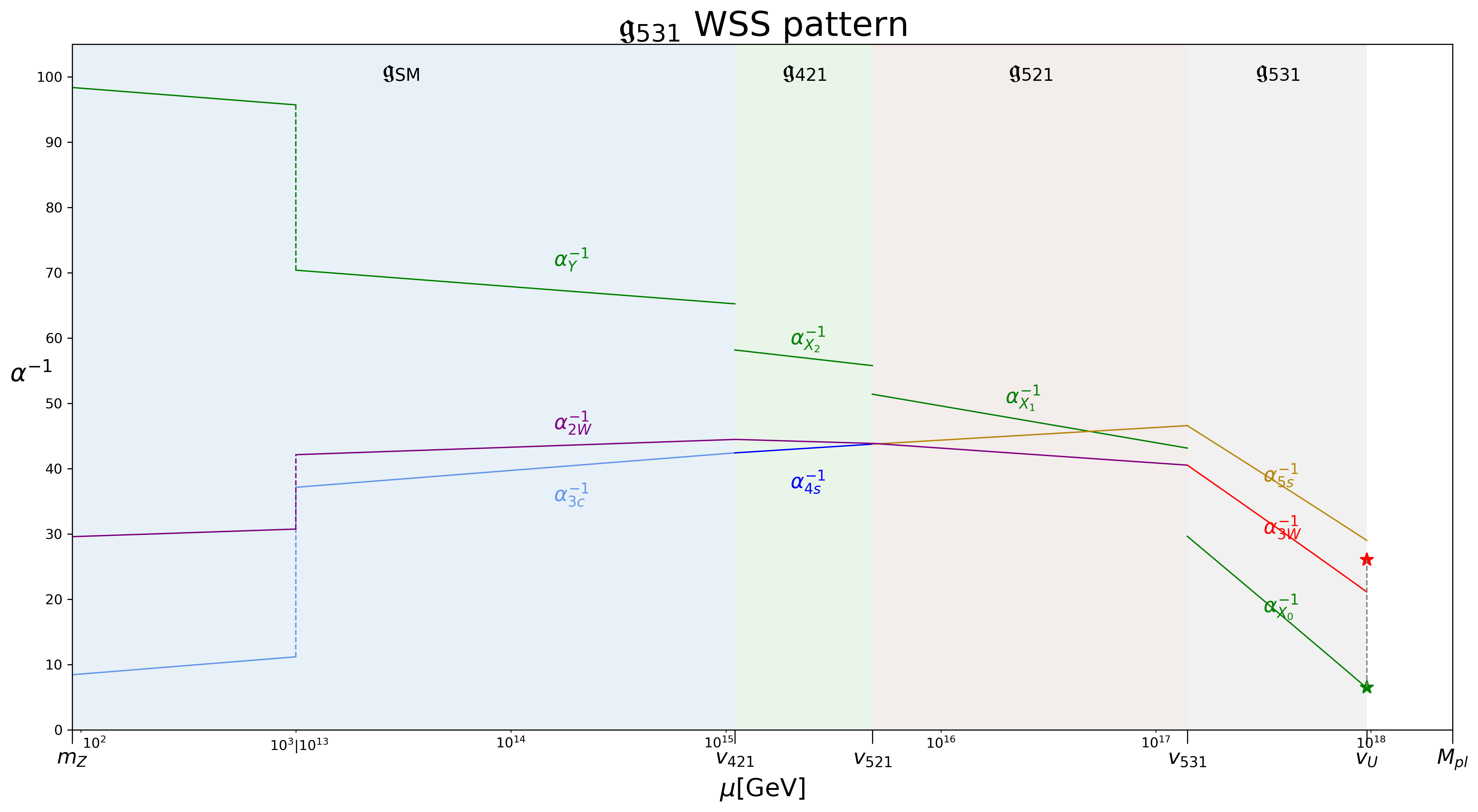
Figure 3: The two-loop RGEs of the ${\mathfrak{s}\mathfrak{u}}(8)$ setup according to the WSS symmetry breaking pattern. The RG evolutions within $10^{3}\,{\rm GeV}\lesssim\mu\lesssim 10^{13}\,{\rm GeV}$ are zoomed out in order to highlight the behaviors in three intermediate symmetry breaking scales given by the benchmark point in Eq. (187).

With the one- and two-loop $\beta$ coefficients defined in Eqs. (4.3), (4.3), (4.3), and (2.3), we plot the RGEs of the ${\mathfrak{s}\mathfrak{u}}(8)$ setup along the WSS symmetry breaking pattern in Fig. 3. The discontinuities of the ${\mathfrak{u}}(1)$ gauge couplings at three intermediate scales follow from their definitions in Eqs. (55), (58), (59), respectively. The benchmark point in Fig. 3 is marked by $\star$ and reads

$$c_{\rm HSW}\approx-1.47\,,\penalty 10000\ v_{U}\approx 9.56\times 10^{17}\,{\rm GeV}\,,$$

$$\alpha_{5c}^{-1}(v_{U})\approx 29.01\,,\penalty 10000\ \alpha_{3W}^{-1}(v_{U})\approx 21.14\,,\penalty 10000\ \alpha_{X_{0}}^{-1}(v_{U})\approx 6.42\,.$$ (60)

5 The WWW symmetry breaking pattern

5.1 Decompositions of the ${\mathfrak{s}\mathfrak{u}}$(8) fermions

${\mathfrak{s}\mathfrak{u}}(8)$	$\mathfrak{g}_{351}$	$\mathfrak{g}_{341}$	$\mathfrak{g}_{331}$	$\mathfrak{g}_{\rm SM}$
$\mathbf{\overline{8_{F}}}^{\Omega}$	$(\mathbf{\overline{3}}\,,\mathbf{1}\,,+\frac{1}{3})_{\mathbf{F}}^{\Omega}$	$(\mathbf{\overline{3}}\,,\mathbf{1}\,,+\frac{1}{3})_{\mathbf{F}}^{\Omega}$	$(\mathbf{\overline{3}}\,,\mathbf{1}\,,+\frac{1}{3})_{\mathbf{F}}^{\Omega}$	$(\mathbf{\overline{3}}\,,\mathbf{1}\,,+\frac{1}{3})_{\mathbf{F}}^{\Omega}\penalty 10000\ :\penalty 10000\ {\mathcal{D}_{R}^{\Omega}}^{c}$
	$(\mathbf{1}\,,\mathbf{\overline{5}}\,,-\frac{1}{5})_{\mathbf{F}}^{\Omega}$	$(\mathbf{1}\,,\mathbf{\overline{4}}\,,-\frac{1}{4})_{\mathbf{F}}^{\Omega}$	$(\mathbf{1}\,,\mathbf{\overline{3}}\,,-\frac{1}{3})_{\mathbf{F}}^{\Omega}$	$(\mathbf{1}\,,\mathbf{\overline{2}}\,,-\frac{1}{2})_{\mathbf{F}}^{\Omega}\penalty 10000\ :\penalty 10000\ \mathcal{L}_{L}^{\Omega}=(\mathcal{E}_{L}^{\Omega}\,,-\mathcal{N}_{L}^{\Omega})^{T}$
				$(\mathbf{1}\,,\mathbf{1}\,,0)_{\mathbf{F}}^{\Omega^{\prime}}\penalty 10000\ :\penalty 10000\ \check{\mathcal{N}}_{L}^{\Omega^{\prime}}$
			$(\mathbf{1}\,,\mathbf{1}\,,0)_{\mathbf{F}}^{\Omega^{\prime\prime}}$	$(\mathbf{1}\,,\mathbf{1}\,,0)_{\mathbf{F}}^{\Omega^{\prime\prime}}\penalty 10000\ :\penalty 10000\ \check{\mathcal{N}}_{L}^{\Omega^{\prime\prime}}$
		$(\mathbf{1}\,,\mathbf{1}\,,0)_{\mathbf{F}}^{\Omega}$	$(\mathbf{1}\,,\mathbf{1}\,,0)_{\mathbf{F}}^{\Omega}$	$(\mathbf{1}\,,\mathbf{1}\,,0)_{\mathbf{F}}^{\Omega}\penalty 10000\ :\penalty 10000\ \check{\mathcal{N}}_{L}^{\Omega}$

Table 11: The ${\mathfrak{s}\mathfrak{u}}(8)$ fermion representation of $\mathbf{\overline{8_{F}}}^{\Omega}$ under the $\mathfrak{g}_{351}\,,\mathfrak{g}_{341}\,,\mathfrak{g}_{331}\,,\mathfrak{g}_{\rm SM}$ subalgebras.

${\mathfrak{s}\mathfrak{u}}(8)$	$\mathfrak{g}_{351}$	$\mathfrak{g}_{341}$	$\mathfrak{g}_{331}$	$\mathfrak{g}_{\rm SM}$
$\mathbf{28_{F}}$	$(\mathbf{\overline{3}}\,,\mathbf{1}\,,-\frac{2}{3})_{\mathbf{F}}$	$(\mathbf{\overline{3}}\,,\mathbf{1}\,,-\frac{2}{3})_{\mathbf{F}}$	$(\mathbf{\overline{3}}\,,\mathbf{1}\,,-\frac{2}{3})_{\mathbf{F}}$	$\underline{(\mathbf{\overline{3}}\,,\mathbf{1}\,,-\frac{2}{3})_{\mathbf{F}}\penalty 10000\ :\penalty 10000\ {t_{R}}^{c}}$
	$(\mathbf{3}\,,\mathbf{5}\,,-\frac{2}{15})_{\mathbf{F}}$	$(\mathbf{3}\,,\mathbf{4}\,,-\frac{1}{12})_{\mathbf{F}}$	$(\mathbf{3}\,,\mathbf{3}\,,0)_{\mathbf{F}}$	$\underline{(\mathbf{3}\,,\mathbf{2}\,,+\frac{1}{6})_{\mathbf{F}}\penalty 10000\ :\penalty 10000\ (t_{L}\,,b_{L})^{T}}$
				$(\mathbf{3}\,,\mathbf{1}\,,-\frac{1}{3})_{\mathbf{F}}^{\prime}\penalty 10000\ :\penalty 10000\ \mathfrak{D}_{L}^{\prime}$
			$(\mathbf{3}\,,\mathbf{1}\,,-\frac{1}{3})_{\mathbf{F}}^{\prime\prime}$	$(\mathbf{3}\,,\mathbf{1}\,,-\frac{1}{3})_{\mathbf{F}}^{\prime\prime}\penalty 10000\ :\penalty 10000\ \mathfrak{D}_{L}^{\prime\prime}$
		$(\mathbf{3}\,,\mathbf{1}\,,-\frac{1}{3})_{\mathbf{F}}$	$(\mathbf{3}\,,\mathbf{1}\,,-\frac{1}{3})_{\mathbf{F}}$	$(\mathbf{3}\,,\mathbf{1}\,,-\frac{1}{3})_{\mathbf{F}}\penalty 10000\ :\penalty 10000\ \mathfrak{D}_{L}$
	$(\mathbf{1}\,,\mathbf{10}\,,+\frac{2}{5})_{\mathbf{F}}$	$(\mathbf{1}\,,\mathbf{4}\,,+\frac{1}{4})_{\mathbf{F}}$	$(\mathbf{1}\,,\mathbf{3}\,,+\frac{1}{3})_{\mathbf{F}}$	$(\mathbf{1}\,,\mathbf{2}\,,+\frac{1}{2})_{\mathbf{F}}^{\prime\prime}\penalty 10000\ :\penalty 10000\ ({\mathfrak{e}_{R}^{\prime\prime}}^{c}\,,{\mathfrak{n}_{R}^{\prime\prime}}^{c})^{T}$
				$(\mathbf{1}\,,\mathbf{1}\,,0)_{\mathbf{F}}^{\prime}\penalty 10000\ :\penalty 10000\ \check{\mathfrak{n}}_{R}^{\prime\,c}$
			$(\mathbf{1}\,,\mathbf{1}\,,0)_{\mathbf{F}}^{\prime\prime}$	$(\mathbf{1}\,,\mathbf{1}\,,0)_{\mathbf{F}}^{\prime\prime}\penalty 10000\ :\penalty 10000\ \check{\mathfrak{n}}_{R}^{\prime\prime\,c}$
		$(\mathbf{1}\,,\mathbf{6}\,,+\frac{1}{2})_{\mathbf{F}}$	$(\mathbf{1}\,,\mathbf{3}\,,+\frac{1}{3})_{\mathbf{F}}^{\prime}$	$(\mathbf{1}\,,\mathbf{1}\,,0)_{\mathbf{F}}^{\prime\prime}\penalty 10000\ :\penalty 10000\ \check{\mathfrak{n}}_{R}^{c}$
				$(\mathbf{1}\,,\mathbf{2}\,,+\frac{1}{2})_{\mathbf{F}}\penalty 10000\ :\penalty 10000\ ({\mathfrak{e}_{R}}^{c}\,,{\mathfrak{n}_{R}}^{c})^{T}$
			$(\mathbf{1}\,,\mathbf{\overline{3}}\,,+\frac{2}{3})_{\mathbf{F}}$	$\underline{(\mathbf{1}\,,\mathbf{1}\,,+1)_{\mathbf{F}}\penalty 10000\ :\penalty 10000\ {\tau_{R}}^{c}}$
				$(\mathbf{1}\,,\mathbf{\overline{2}}\,,+\frac{1}{2})_{\mathbf{F}}^{\prime}\penalty 10000\ :\penalty 10000\ (\mathfrak{n}_{R}^{\prime\,c}\,,-\mathfrak{e}_{R}^{\prime\,c})^{T}$

Table 12: The ${\mathfrak{s}\mathfrak{u}}(8)$ fermion representation of $\mathbf{28_{F}}$ under the $\mathfrak{g}_{351}\,,\mathfrak{g}_{341}\,,\mathfrak{g}_{331}\,,\mathfrak{g}_{\rm SM}$ subalgebras. All IRs for SM fermions are marked with underlines.

${\mathfrak{s}\mathfrak{u}}(8)$	$\mathfrak{g}_{351}$	$\mathfrak{g}_{341}$	$\mathfrak{g}_{331}$	$\mathfrak{g}_{\rm SM}$
$\mathbf{56_{F}}$	$(\mathbf{\overline{3}}\,,\mathbf{5}\,,-\frac{7}{15})_{\mathbf{F}}$	$(\mathbf{\overline{3}}\,,\mathbf{4}\,,-\frac{5}{12})_{\mathbf{F}}$	$(\mathbf{\overline{3}}\,,\mathbf{3}\,,-\frac{1}{3})_{\mathbf{F}}$	$(\mathbf{\overline{3}}\,,\mathbf{2}\,,-\frac{1}{6})_{\mathbf{F}}\penalty 10000\ :\penalty 10000\ ({\mathfrak{d}_{R}}^{c}\,,{\mathfrak{u}_{R}}^{c})^{T}$
				$(\mathbf{\overline{3}}\,,\mathbf{1}\,,-\frac{2}{3})_{\mathbf{F}}^{\prime}\penalty 10000\ :\penalty 10000\ {\mathfrak{U}_{R}}^{c}$
			$(\mathbf{\overline{3}}\,,\mathbf{1}\,,-\frac{2}{3})_{\mathbf{F}}^{\prime\prime}$	$\underline{(\mathbf{\overline{3}}\,,\mathbf{1}\,,-\frac{2}{3})_{\mathbf{F}}^{\prime\prime}\penalty 10000\ :\penalty 10000\ {c_{R}}^{c}}$
		$(\mathbf{\overline{3}}\,,\mathbf{1}\,,-\frac{2}{3})_{\mathbf{F}}^{\prime\prime\prime}$	$(\mathbf{\overline{3}}\,,\mathbf{1}\,,-\frac{2}{3})_{\mathbf{F}}^{\prime\prime\prime}$	$\underline{(\mathbf{\overline{3}}\,,\mathbf{1}\,,-\frac{2}{3})_{\mathbf{F}}^{\prime\prime\prime}\penalty 10000\ :\penalty 10000\ {u_{R}}^{c}}$
	$(\mathbf{1}\,,\mathbf{\overline{10}}\,,+\frac{3}{5})_{\mathbf{F}}$	$(\mathbf{1}\,,\mathbf{\overline{4}}\,,+\frac{3}{4})_{\mathbf{F}}$	$(\mathbf{1}\,,\mathbf{\overline{3}}\,,+\frac{2}{3})_{\mathbf{F}}^{\prime}$	$(\mathbf{1}\,,\mathbf{\overline{2}}\,,+\frac{1}{2})_{\mathbf{F}}\penalty 10000\ :\penalty 10000\ ({\mathfrak{n}_{R}^{\prime\prime\prime}}^{c}\,,-{\mathfrak{e}_{R}^{\prime\prime\prime}}^{c})^{T}$
				$\underline{(\mathbf{1}\,,\mathbf{1}\,,+1)_{\mathbf{F}}^{\prime}\penalty 10000\ :\penalty 10000\ {\mu_{R}}^{c}}$
			$(\mathbf{1}\,,\mathbf{1}\,,+1)_{\mathbf{F}}^{\prime\prime}$	$(\mathbf{1}\,,\mathbf{1}\,,+1)_{\mathbf{F}}^{\prime\prime}\penalty 10000\ :\penalty 10000\ {\mathfrak{E}_{R}}^{\,c}$
		$(\mathbf{1}\,,\mathbf{6}\,,+\frac{1}{2})_{\mathbf{F}}^{\prime}$	$(\mathbf{1}\,,\mathbf{3}\,,+\frac{1}{3})_{\mathbf{F}}^{\prime\prime}$	$(\mathbf{1}\,,\mathbf{2}\,,+\frac{1}{2})_{\mathbf{F}}^{\prime\prime\prime\prime}\penalty 10000\ :\penalty 10000\ ({\mathfrak{e}_{R}^{\prime\prime\prime\prime}}^{c}\,,{\mathfrak{n}_{R}^{\prime\prime\prime\prime}}^{c})^{T}$
				$(\mathbf{1}\,,\mathbf{1}\,,0)_{\mathbf{F}}^{\prime\prime\prime}\penalty 10000\ :\penalty 10000\ {\check{\mathfrak{n}}_{R}}^{\prime\prime\prime\,c}$
			$(\mathbf{1}\,,\mathbf{\overline{3}}\,,+\frac{2}{3})_{\mathbf{F}}^{\prime\prime}$	$(\mathbf{1}\,,\mathbf{\overline{2}}\,,+\frac{1}{2})_{\mathbf{F}}^{\prime\prime\prime\prime\prime}\penalty 10000\ :\penalty 10000\ ({\mathfrak{n}_{R}^{\prime\prime\prime\prime\prime}}^{c}\,,-{\mathfrak{e}_{R}^{\prime\prime\prime\prime\prime}}^{c})^{T}$
				$\underline{(\mathbf{1}\,,\mathbf{1}\,,+1)_{\mathbf{F}}^{\prime\prime\prime}\penalty 10000\ :\penalty 10000\ {e_{R}}^{c}}$
	$(\mathbf{3}\,,\mathbf{10}\,,+\frac{1}{15})_{\mathbf{F}}$	$(\mathbf{3}\,,\mathbf{4}\,,-\frac{1}{12})_{\mathbf{F}}^{\prime}$	$(\mathbf{3}\,,\mathbf{3}\,,0)_{\mathbf{F}}^{\prime}$	$(\mathbf{3}\,,\mathbf{1}\,,-\frac{1}{3})_{\mathbf{F}}^{\prime\prime\prime\prime}\penalty 10000\ :\penalty 10000\ \mathfrak{D}_{L}^{\prime\prime\prime\prime}$
				$\underline{(\mathbf{3}\,,\mathbf{2}\,,+\frac{1}{6})_{\mathbf{F}}^{\prime}\penalty 10000\ :\penalty 10000\ (u_{L}\,,d_{L})^{T}}$
			$(\mathbf{3}\,,\mathbf{1}\,,-\frac{1}{3})_{\mathbf{F}}^{\prime\prime\prime\prime\prime}$	$(\mathbf{3}\,,\mathbf{1}\,,-\frac{1}{3})_{\mathbf{F}}^{\prime\prime\prime\prime\prime}\penalty 10000\ :\penalty 10000\ \mathfrak{D}_{L}^{\prime\prime\prime\prime\prime}$
		$(\mathbf{3}\,,\mathbf{6}\,,+\frac{1}{6})_{\mathbf{F}}$	$(\mathbf{3}\,,\mathbf{3}\,,0)_{\mathbf{F}}^{\prime\prime}$	$(\mathbf{3}\,,\mathbf{1}\,,-\frac{1}{3})_{\mathbf{F}}^{\prime\prime\prime}\penalty 10000\ :\penalty 10000\ \mathfrak{D}_{L}^{\prime\prime\prime}$
				$\underline{(\mathbf{3}\,,\mathbf{2}\,,+\frac{1}{6})_{\mathbf{F}}^{\prime\prime}\penalty 10000\ :\penalty 10000\ (c_{L}\,,s_{L})^{T}}$
			$(\mathbf{3}\,,\mathbf{\overline{3}}\,,+\frac{1}{3})_{\mathbf{F}}$	$(\mathbf{3}\,,\mathbf{1}\,,+\frac{2}{3})_{\mathbf{F}}\penalty 10000\ :\penalty 10000\ \mathfrak{U}_{L}$
				$(\mathbf{3}\,,\mathbf{\overline{2}}\,,+\frac{1}{6})_{\mathbf{F}}^{\prime\prime\prime}\penalty 10000\ :\penalty 10000\ (\mathfrak{d}_{L}\,,-\mathfrak{u}_{L})^{T}$
	$(\mathbf{1}\,,\mathbf{1}\,,-1)_{\mathbf{F}}$	$(\mathbf{1}\,,\mathbf{1}\,,-1)_{\mathbf{F}}$	$(\mathbf{1}\,,\mathbf{1}\,,-1)_{\mathbf{F}}$	$(\mathbf{1}\,,\mathbf{1}\,,-1)_{\mathbf{F}}\penalty 10000\ :\penalty 10000\ {\mathfrak{E}_{L}}$

Table 13: The ${\mathfrak{s}\mathfrak{u}}(8)$ fermion representation of $\mathbf{56_{F}}$ under the $\mathfrak{g}_{351}\,,\mathfrak{g}_{341}\,,\mathfrak{g}_{331}\,,\mathfrak{g}_{\rm SM}$ subalgebras. All IRs for SM fermions are marked with underlines.

By following the WWW symmetry breaking pattern in Eq. (13d), we tabulate the fermion representations at various stages in Tables 11, 12, and 13. Along this pattern, the global $\widetilde{{\rm U}}(1)_{T}$ symmetry evolves to the global $\widetilde{{\rm U}}(1)_{B-L}$ at the EW scale according to the following sequence:

$$\mathfrak{g}_{351}\penalty 10000\ :\penalty 10000\ \mathcal{T}^{\prime}\equiv\mathcal{T}+5\mathcal{X}_{0}\,,\quad\mathfrak{g}_{341}\penalty 10000\ :\penalty 10000\ \mathcal{T}^{\prime\prime}\equiv\mathcal{T}^{\prime}\,,$$

$$\mathfrak{g}_{331}\penalty 10000\ :\penalty 10000\ \mathcal{T}^{\prime\prime\prime}\equiv\mathcal{T}^{\prime\prime}\,,\quad\mathfrak{g}_{\rm SM}\penalty 10000\ :\penalty 10000\ \mathcal{B}-\mathcal{L}\equiv\mathcal{T}^{\prime\prime\prime}\,.$$ (61)

5.2 Decompositions of the ${\mathfrak{s}\mathfrak{u}}$(8) Higgs fields

We decompose the Higgs fields in Eq. (6) into components that can be responsible for the sequential symmetry breaking stages in Eq. (13d). For Higgs fields of $\mathbf{\overline{8_{H}}}_{\,,\omega}$, they read

$$\mathbf{\overline{8_{H}}}_{\,,\omega} \supset \langle(\mathbf{1}\,,\mathbf{\overline{5}}\,,-\frac{1}{5})_{\mathbf{H}\,,\omega}\rangle\supset\langle(\mathbf{1}\,,\mathbf{\overline{4}}\,,-\frac{1}{4})_{\mathbf{H}\,,\omega}\rangle\supset\langle(\mathbf{1}\,,\mathbf{\overline{3}}\,,-\frac{1}{3})_{\mathbf{H}\,,\omega}\rangle\,.$$ (62)

For Higgs fields of $\mathbf{\overline{28_{H}}}_{\,,\dot{\omega}}$, they read

$$\mathbf{\overline{28_{H}}}_{\,,\dot{\omega}} \supset \underline{(\mathbf{1}\,,\mathbf{\overline{10}}\,,-\frac{2}{5})_{\mathbf{H}\,,\dot{\omega}}}$$ (63)

$$\supset \underline{(\mathbf{1}\,,\mathbf{\overline{6}}\,,-\frac{1}{2})_{\mathbf{H}\,,\dot{\omega}}}\oplus\langle(\mathbf{1}\,,\mathbf{\overline{4}}\,,-\frac{1}{4})_{\mathbf{H}\,,\dot{\omega}}\rangle$$

$$\supset \Big[\underline{(\mathbf{1}\,,\mathbf{3}\,,-\frac{2}{3})_{\mathbf{H}\,,\dot{\omega}}}\oplus\langle(\mathbf{1}\,,\mathbf{\overline{3}}\,,-\frac{1}{3})_{\mathbf{H}\,,\dot{\omega}}\rangle\Big]\oplus\langle(\mathbf{1}\,,\mathbf{\overline{3}}\,,-\frac{1}{3})_{\mathbf{H}\,,\dot{\omega}}^{\prime}\rangle\,.$$

For Higgs field of $\mathbf{70_{H}}$, it reads

$$\mathbf{70_{H}} \supset (\mathbf{1}\,,\mathbf{5}\,,-\frac{4}{5})_{\mathbf{H}}\oplus\underline{(\mathbf{1}\,,\mathbf{\overline{5}}\,,+\frac{4}{5})_{\mathbf{H}}}\oplus(\mathbf{3}\,,\mathbf{\overline{10}}\,,+\frac{4}{15})_{\mathbf{H}}\oplus(\mathbf{\overline{3}}\,,\mathbf{10}\,,-\frac{4}{15})_{\mathbf{H}}$$ (64)

$$\supset \underline{(\mathbf{1}\,,\mathbf{\overline{4}}\,,+\frac{3}{4})_{\mathbf{H}}}\supset\underline{(\mathbf{1}\,,\mathbf{\overline{3}}\,,+\frac{2}{3})_{\mathbf{H}}}\supset\langle(\mathbf{1}\,,\mathbf{\overline{2}}\,,+\frac{1}{2})_{\mathbf{H}}\rangle\,.$$

5.3 RGEs of the WWW symmetry breaking pattern

Between the $v_{351}\leq\mu\leq v_{U}$, almost all massless Higgs fields are summarized as follows:

$$(\mathbf{\overline{3}}\,,\mathbf{1}\,,+\frac{1}{3})_{\mathbf{H}\,,\omega}\oplus(\mathbf{1}\,,\mathbf{\overline{5}}\,,-\frac{1}{5})_{\mathbf{H}\,,\omega}\subset\mathbf{\overline{8_{H}}}_{,\omega}\,,$$

$$(\mathbf{3}\,,\mathbf{1}\,,+\frac{2}{3})_{\mathbf{H}\,,\dot{\omega}}\oplus(\mathbf{\overline{3}}\,,\mathbf{\overline{5}}\,,+\frac{2}{15})_{\mathbf{H}\,,\dot{\omega}}\oplus(\mathbf{1}\,,\mathbf{\overline{10}}\,,-\frac{2}{5})_{\mathbf{H}\,,\dot{\omega}}\subset\mathbf{\overline{28_{H}}}_{,\dot{\omega}}\,,$$

$$(\mathbf{1}\,,\mathbf{5}\,,-\frac{4}{5})_{\mathbf{H}}\oplus(\mathbf{1}\,,\mathbf{\overline{5}}\,,+\frac{4}{5})_{\mathbf{H}}\oplus(\mathbf{3}\,,\mathbf{\overline{10}}\,,+\frac{4}{15})_{\mathbf{H}}\oplus(\mathbf{\overline{3}}\,,\mathbf{10}\,,-\frac{4}{15})_{\mathbf{H}}\subset\mathbf{70_{H}}\,,$$

$$(\mathbf{1}\,,\mathbf{\overline{5}}\,,+\frac{4}{5})_{\mathbf{H}}\oplus(\mathbf{1}\,,\mathbf{5}\,,-\frac{4}{5})_{\mathbf{H}}\oplus(\mathbf{\overline{3}}\,,\mathbf{10}\,,-\frac{4}{15})_{\mathbf{H}}\oplus(\mathbf{3}\,,\mathbf{\overline{10}}\,,+\frac{4}{15})_{\mathbf{H}}\subset\mathbf{\overline{70_{H}}}\,,$$

$$(\mathbf{3}\,,\mathbf{1}\,,-\frac{1}{3})_{\mathbf{H}}^{\omega}\oplus(\mathbf{1}\,,\mathbf{5}\,,+\frac{1}{5})_{\mathbf{H}}^{\omega}\subset\mathbf{8_{H}}^{\omega}\,,$$

$$(\mathbf{\overline{3}}\,,\mathbf{1}\,,-\frac{2}{3})_{\mathbf{H}}^{\dot{\omega}}\oplus(\mathbf{3}\,,\mathbf{5}\,,-\frac{2}{15})_{\mathbf{H}}^{\dot{\omega}}\oplus(\mathbf{1}\,,\mathbf{10}\,,+\frac{2}{5})_{\mathbf{H}}^{\dot{\omega}}\subset\mathbf{28_{H}}^{\dot{\omega}}\,.$$ (65)

All fermionic components of $\mathbf{\overline{8_{F}}}^{\Omega}\oplus\mathbf{28_{F}}\oplus\mathbf{56_{F}}$ remain massless after the decomposition into the $\mathfrak{g}_{351}$ IRs. Consequently, we have the $\mathfrak{g}_{351}$ $\beta$ coefficients of

$$(b^{(1)}_{{\mathfrak{s}\mathfrak{u}}(3)_{c}}\,,b^{(1)}_{{\mathfrak{s}\mathfrak{u}}(5)_{W}}\,,b^{(1)}_{{\mathfrak{u}}(1)_{X_{0}}})=(+60\,,+54\,,+\frac{368}{5})\,,$$

$$b^{(2)}_{\mathcal{G}_{351}}=\begin{pmatrix}728&648&352/15\\ 216&6984/5&672/25\\ 2816/15&16128/25&98816/1125\end{pmatrix}\,.$$ (66)

Between the $v_{341}\leq\mu\leq v_{351}$, the massless Higgs fields are

$$(\mathbf{\overline{3}}\,,\mathbf{1}\,,+\frac{1}{3})_{\mathbf{H}\,,3,\rm V,\rm VI}\oplus(\mathbf{1}\,,\mathbf{\overline{4}}\,,-\frac{1}{4})_{\mathbf{H}\,,3,\rm V,\rm VI}\subset...\subset\mathbf{\overline{8_{H}}}_{\,,3,\rm V,\rm VI}\,,$$ (67)

$$(\mathbf{3}\,,\mathbf{1}\,,+\frac{2}{3})_{\mathbf{H}\,,\dot{\omega}}\oplus\Big[(\mathbf{\overline{3}}\,,\mathbf{\overline{4}}\,,+\frac{1}{12})_{\mathbf{H}\,,\dot{\omega}}\oplus(\mathbf{\overline{3}}\,,\mathbf{1}\,,+\frac{1}{3})_{\mathbf{H}\,,\dot{\omega}}\Big]$$

$$\oplus \Big[(\mathbf{1}\,,\mathbf{\overline{4}}\,,-\frac{1}{4})_{\mathbf{H}\,,\dot{\omega}}\oplus(\mathbf{1}\,,\mathbf{6}\,,-\frac{1}{2})_{\mathbf{H}\,,\dot{\omega}}\Big]\subset...\subset\mathbf{\overline{28_{H}}}_{\,,\dot{\omega}}\,,\quad\dot{\omega}=(\dot{1},\dot{2},\dot{\rm VII},\dot{\rm VIII},\dot{\rm IX})\,,$$

$$(\mathbf{\overline{3}}\,,\mathbf{1}\,,-\frac{2}{3})_{\mathbf{H}}^{\dot{\rm VII}}\oplus\Big[(\mathbf{3}\,,\mathbf{4}\,,-\frac{1}{12})_{\mathbf{H}}^{\dot{\rm VII}}\oplus(\mathbf{3}\,,\mathbf{1}\,,-\frac{1}{3})_{\mathbf{H}}^{\dot{\rm VII}}\Big]$$

$$\oplus \Big[(\mathbf{1}\,,\mathbf{4}\,,+\frac{1}{4})_{\mathbf{H}}^{\dot{\rm VII}}\oplus(\mathbf{1}\,,\mathbf{6}\,,+\frac{1}{2})_{\mathbf{H}}^{\dot{\rm VII}}\Big]\subset...\subset\mathbf{28_{H}}^{\dot{\rm VII}}\,,$$

$$(\mathbf{1}\,,\mathbf{\overline{4}}\,,+\frac{3}{4})_{\mathbf{H}}\subset...\subset\mathbf{70_{H}}\,.$$

All ${\mathfrak{s}\mathfrak{u}}$(8) fermions in Eq. (191) remain massless after the decomposition into the $\mathfrak{g}_{341}$ IRs. Consequently, we have the $\mathfrak{g}_{341}$ $\beta$ coefficients of

$$(b^{(1)}_{{\mathfrak{s}\mathfrak{u}}(3)_{c}}\,,b^{(1)}_{{\mathfrak{s}\mathfrak{u}}(4)_{W}}\,,b^{(1)}_{{\mathfrak{u}}(1)_{X_{1}}})=(+\frac{29}{6}\,,+\frac{4}{3}\,,+\frac{173}{9})\,,$$

$$b^{(2)}_{\mathfrak{g}_{341}}=\begin{pmatrix}655/3&255/2&373/36\\ 68&3389/12&271/24\\ 746/9&1355/8&17363/432\end{pmatrix}\,.$$ (68)

The ${\mathfrak{s}\mathfrak{u}}(5)_{W}\oplus{\mathfrak{u}}(1)_{X_{0}}$ gauge couplings match with the ${\mathfrak{s}\mathfrak{u}}(4)_{W}\oplus{\mathfrak{u}}(1)_{X_{1}}$ gauge couplings as follows:

$$\alpha_{5W}^{-1}(v_{351})=\alpha_{4W}^{-1}(v_{351})\,,\penalty 10000\ \alpha_{X_{1}}^{-1}(v_{351})=\frac{1}{10}\alpha_{5W}^{-1}(v_{351})+\alpha_{X_{0}}^{-1}(v_{351})\,.$$ (69)

Between the $v_{331}\leq\mu\leq v_{341}$, the massless Higgs fields are

$$(\mathbf{\overline{3}}\,,\mathbf{1}\,,+\frac{1}{3})_{\mathbf{H}\,,3,\rm VI}\oplus(\mathbf{1}\,,\mathbf{\overline{3}}\,,-\frac{1}{3})_{\mathbf{H}\,,3,\rm VI}\subset...\subset\mathbf{\overline{8_{H}}}_{,3,\rm VI}\,,$$ (70)

$$(\mathbf{3}\,,\mathbf{1}\,,+\frac{2}{3})_{\mathbf{H}\,,\dot{\omega}}\oplus\Big[(\mathbf{\overline{3}}\,,\mathbf{1}\,,+\frac{1}{3})_{\mathbf{H}\,,\dot{\omega}}\oplus(\mathbf{\overline{3}}\,,\mathbf{1}\,,+\frac{1}{3})_{\mathbf{H}\,,\dot{\omega}}^{\prime}\oplus(\mathbf{\overline{3}}\,,\mathbf{\overline{3}}\,,0)_{\mathbf{H}\,,\dot{\omega}}\Big]$$

$$\oplus \Big[(\mathbf{1}\,,\mathbf{\overline{3}}\,,-\frac{1}{3})_{\mathbf{H}\,,\dot{\omega}}\oplus(\mathbf{1}\,,\mathbf{\overline{3}}\,,-\frac{1}{3})_{\mathbf{H}\,,\dot{\omega}}^{\prime}\oplus(\mathbf{1}\,,\mathbf{3}\,,-\frac{2}{3})_{\mathbf{H}\,,\dot{\omega}}\Big]\subset...\subset\mathbf{\overline{28_{H}}}_{\,,\dot{\omega}}\,,\quad\dot{\omega}=(\dot{2},\dot{\rm VIII},\dot{\rm IX})\,,$$

$$(\mathbf{1}\,,\mathbf{\overline{3}}\,,+\frac{2}{3})_{\mathbf{H}}\subset...\subset\mathbf{70_{H}}\,.$$

All ${\mathfrak{s}\mathfrak{u}}$(8) fermions in Eq. (195) remain massless after the decomposition into the $\mathfrak{g}_{331}$ IRs. Consequently, we have the $\mathfrak{g}_{331}$ $\beta$ coefficients of

$$(b^{(1)}_{{\mathfrak{s}\mathfrak{u}}(3)_{c}}\,,b^{(1)}_{{\mathfrak{s}\mathfrak{u}}(3)_{W}}\,,b^{(1)}_{{\mathfrak{u}}(1)_{X_{2}}})=(-\frac{5}{3}\,,-\frac{3}{2}\,,+\frac{122}{9})\,,$$

$$b^{(2)}_{\mathfrak{g}_{331}}=\begin{pmatrix}256/3&36&58/9\\ 36&89&22/3\\ 464/9&176/3&782/27\end{pmatrix}\,.$$ (71)

The ${\mathfrak{s}\mathfrak{u}}(4)_{W}\oplus{\mathfrak{u}}(1)_{X_{1}}$ gauge couplings match with the ${\mathfrak{s}\mathfrak{u}}(3)_{W}\oplus{\mathfrak{u}}(1)_{X_{2}}$ gauge couplings as follows:

$$\alpha_{4W}^{-1}(v_{341})=\alpha_{3W}^{-1}(v_{341})\,,\penalty 10000\ \alpha_{X_{2}}^{-1}(v_{341})=\frac{1}{6}\alpha_{4W}^{-1}(v_{341})+\alpha_{X_{1}}^{-1}(v_{341})\,.$$ (72)

Between the $v_{\rm EW}\leq\mu\leq v_{331}$, we have the same $\mathfrak{g}_{\rm SM}$ $\beta$ coefficients as Eq. (2.3). The ${\mathfrak{s}\mathfrak{u}}(3)_{W}\oplus{\mathfrak{u}}(1)_{X_{2}}$ gauge couplings match with the ${\mathfrak{s}\mathfrak{u}}(2)_{W}\oplus{\mathfrak{u}}(1)_{Y}$ gauge couplings as follows:

$$\alpha_{3W}^{-1}(v_{331})=\alpha_{2W}^{-1}(v_{331})\,,\penalty 10000\ \alpha_{\rm Y}^{-1}(v_{331})=\frac{1}{3}\alpha_{3W}^{-1}(v_{331})+\alpha_{X_{2}}^{-1}(v_{331})\,.$$ (73)

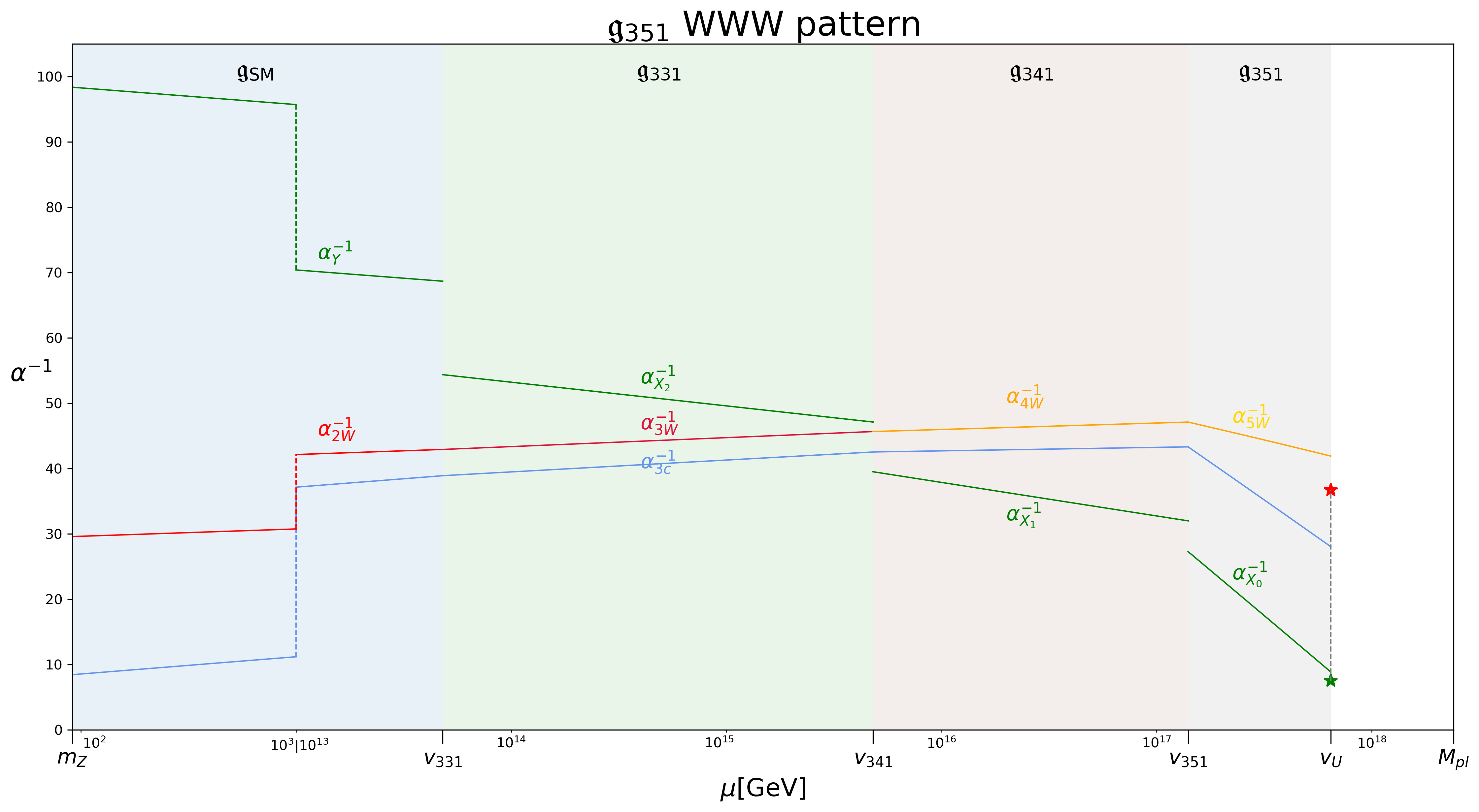
Figure 4: The two-loop RGEs of the ${\mathfrak{s}\mathfrak{u}}(8)$ setup according to the WSS symmetry breaking pattern. The RG evolutions within $10^{3}\,{\rm GeV}\lesssim\mu\lesssim 10^{13}\,{\rm GeV}$ are zoomed out in order to highlight the behaviors in three intermediate symmetry breaking scales given by the benchmark point in Eq. (216).

With the one- and two-loop $\beta$ coefficients defined in Eqs. (5.3), (5.3), (5.3), and (2.3), we plot the RGEs of the ${\mathfrak{s}\mathfrak{u}}(8)$ setup along the WWW symmetry breaking pattern in Fig. 4. The discontinuities of the $\mathfrak{u}(1)$ gauge couplings at three intermediate scales follow from their definitions in Eqs. (69), (72), and (73). The benchmark point in Fig. 4 is marked by $\star$ and reads

$$c_{\rm HSW}\approx 4.16\,,\penalty 10000\ v_{U}\approx 4.42\times 10^{17}\,{\rm GeV}\,,$$

$$\alpha_{3c}^{-1}(v_{U})\approx 25.41\,,\penalty 10000\ \alpha_{5W}^{-1}(v_{U})\approx 38.75\,,\penalty 10000\ \alpha_{X_{0}}^{-1}(v_{U})\approx 8.11\,.$$ (74)

6 The no-go pattern of ${\mathfrak{s}\mathfrak{u}}(8)\to\mathfrak{g}_{621}$

In this section, we prove that the non-maximal symmetry breaking pattern of ${\mathfrak{s}\mathfrak{u}}(8)\to\mathfrak{g}_{621}$ cannot be realistic, since the vectorlike quarks of $(\mathfrak{u}\,,\mathfrak{d})$ from the $\mathbf{56_{F}}$ are massless at the EWSB scale. For this purpose, we only tabulate the fermion representation of $\mathbf{56_{F}}$ at various stages in Table 14 by following the SSS symmetry breaking pattern in Eq. (11c).

${\mathfrak{s}\mathfrak{u}}(8)$	$\mathfrak{g}_{621}$	$\mathfrak{g}_{521}$	$\mathfrak{g}_{421}$	$\mathfrak{g}_{\rm SM}$
$\mathbf{56_{F}}$	$(\mathbf{20}\,,\mathbf{1}\,,-\frac{1}{2})_{\mathbf{F}}$	$(\mathbf{\overline{10}}\,,\mathbf{1}\,,-\frac{3}{5})_{\mathbf{F}}$	$(\mathbf{\overline{4}}\,,\mathbf{1}\,,-\frac{3}{4})_{\mathbf{F}}$	$(\mathbf{\overline{3}}\,,\mathbf{1}\,,-\frac{2}{3})_{\mathbf{F}}^{\prime}\penalty 10000\ :\penalty 10000\ {\mathfrak{U}_{R}}^{c}$
				$(\mathbf{1}\,,\mathbf{1}\,,-1)_{\mathbf{F}}\penalty 10000\ :\penalty 10000\ \mathfrak{E}_{L}$
			$(\mathbf{6}\,,\mathbf{1}\,,-\frac{1}{2})_{\mathbf{F}}^{\prime}$	$\underline{(\mathbf{\overline{3}}\,,\mathbf{1}\,,-\frac{2}{3})_{\mathbf{F}}^{\prime\prime}\penalty 10000\ :\penalty 10000\ {u_{R}}^{c}}$
				$(\mathbf{3}\,,\mathbf{1}\,,-\frac{1}{3})_{\mathbf{F}}^{\prime\prime\prime}\penalty 10000\ :\penalty 10000\ \mathfrak{D}_{L}^{\prime\prime\prime}$
		$(\mathbf{10}\,,\mathbf{1}\,,-\frac{2}{5})_{\mathbf{F}}^{\prime}$	$(\mathbf{6}\,,\mathbf{1}\,,-\frac{1}{2})_{\mathbf{F}}^{\prime\prime}$	$\underline{(\mathbf{\overline{3}}\,,\mathbf{1}\,,-\frac{2}{3})_{\mathbf{F}}^{\prime\prime\prime}\penalty 10000\ :\penalty 10000\ {c_{R}}^{c}}$
				$(\mathbf{3}\,,\mathbf{1}\,,-\frac{1}{3})_{\mathbf{F}}^{\prime\prime\prime\prime}\penalty 10000\ :\penalty 10000\ \mathfrak{D}_{L}^{\prime\prime\prime\prime}$
			$(\mathbf{4}\,,\mathbf{1}\,,-\frac{1}{4})_{\mathbf{F}}^{\prime\prime}$	$(\mathbf{3}\,,\mathbf{1}\,,-\frac{1}{3})_{\mathbf{F}}^{\prime\prime\prime\prime\prime}\penalty 10000\ :\penalty 10000\ \mathfrak{D}_{L}^{\prime\prime\prime\prime\prime}$
				$(\mathbf{1}\,,\mathbf{1}\,,0)_{\mathbf{F}}^{\prime\prime\prime}\penalty 10000\ :\penalty 10000\ {\check{\mathfrak{n}}_{R}}^{\prime\prime\prime\,c}$
	$(\mathbf{15}\,,\mathbf{2}\,,+\frac{1}{6})_{\mathbf{F}}$	$(\mathbf{10}\,,\mathbf{2}\,,+\frac{1}{10})_{\mathbf{F}}$	$(\mathbf{6}\,,\mathbf{2}\,,0)_{\mathbf{F}}$	$(\mathbf{\overline{3}}\,,\mathbf{2}\,,-\frac{1}{6})_{\mathbf{F}}\penalty 10000\ :\penalty 10000\ ({\mathfrak{d}_{R}}^{c}\,,{\mathfrak{u}_{R}}^{c})^{T}$
				$(\mathbf{3}\,,\mathbf{2}\,,+\frac{1}{6})_{\mathbf{F}}^{\prime}\penalty 10000\ :\penalty 10000\ (\mathfrak{u}_{L}\,,\mathfrak{d}_{L})^{T}$
			$(\mathbf{4}\,,\mathbf{2}\,,+\frac{1}{4})_{\mathbf{F}}^{\prime}$	$\underline{(\mathbf{3}\,,\mathbf{2}\,,+\frac{1}{6})_{\mathbf{F}}^{\prime\prime}\penalty 10000\ :\penalty 10000\ (c_{L}\,,s_{L})^{T}}$
				$(\mathbf{1}\,,\mathbf{2}\,,+\frac{1}{2})_{\mathbf{F}}^{\prime\prime\prime}\penalty 10000\ :\penalty 10000\ ({\mathfrak{e}_{R}^{\prime\prime\prime}}^{c}\,,{\mathfrak{n}_{R}^{\prime\prime\prime}}^{c})^{T}$
		$(\mathbf{5}\,,\mathbf{2}\,,+\frac{3}{10})_{\mathbf{F}}^{\prime}$	$(\mathbf{4}\,,\mathbf{2}\,,+\frac{1}{4})_{\mathbf{F}}^{\prime\prime}$	$\underline{(\mathbf{3}\,,\mathbf{2}\,,+\frac{1}{6})_{\mathbf{F}}^{\prime\prime\prime}\penalty 10000\ :\penalty 10000\ (u_{L}\,,d_{L})^{T}}$
				$(\mathbf{1}\,,\mathbf{2}\,,+\frac{1}{2})_{\mathbf{F}}^{\prime\prime\prime\prime}\penalty 10000\ :\penalty 10000\ ({\mathfrak{e}_{R}^{\prime\prime\prime\prime}}^{c}\,,{\mathfrak{n}_{R}^{\prime\prime\prime\prime}}^{c})^{T}$
			$(\mathbf{1}\,,\mathbf{2}\,,+\frac{1}{2})_{\mathbf{F}}^{\prime\prime\prime\prime\prime}$	$(\mathbf{1}\,,\mathbf{2}\,,+\frac{1}{2})_{\mathbf{F}}^{\prime\prime\prime\prime\prime}\penalty 10000\ :\penalty 10000\ ({\mathfrak{e}_{R}^{\prime\prime\prime\prime\prime}}^{c}\,,{\mathfrak{n}_{R}^{\prime\prime\prime\prime\prime}}^{c})^{T}$
	$(\mathbf{6}\,,\mathbf{1}\,,+\frac{5}{6})_{\mathbf{F}}$	$(\mathbf{5}\,,\mathbf{1}\,,+\frac{4}{5})_{\mathbf{F}}$	$(\mathbf{4}\,,\mathbf{1}\,,+\frac{3}{4})_{\mathbf{F}}$	$(\mathbf{3}\,,\mathbf{1}\,,+\frac{2}{3})_{\mathbf{F}}\penalty 10000\ :\penalty 10000\ \mathfrak{U}_{L}$
				$(\mathbf{1}\,,\mathbf{1}\,,+1)_{\mathbf{F}}^{\prime}\penalty 10000\ :\penalty 10000\ {\mathfrak{E}_{R}}^{c}$
			$(\mathbf{1}\,,\mathbf{1}\,,+1)_{\mathbf{F}}^{\prime\prime}$	$\underline{(\mathbf{1}\,,\mathbf{1}\,,+1)_{\mathbf{F}}^{\prime\prime}\penalty 10000\ :\penalty 10000\ {\mu_{R}}^{c}}$
		$(\mathbf{1}\,,\mathbf{1}\,,+1)_{\mathbf{F}}^{\prime\prime\prime}$	$(\mathbf{1}\,,\mathbf{1}\,,+1)_{\mathbf{F}}^{\prime\prime\prime}$	$\underline{(\mathbf{1}\,,\mathbf{1}\,,+1)_{\mathbf{F}}^{\prime\prime\prime}\penalty 10000\ :\penalty 10000\ {e_{R}}^{c}}$

Table 14: The ${\mathfrak{s}\mathfrak{u}}(8)$ fermion representation of $\mathbf{56_{F}}$ under the $\mathfrak{g}_{621}\,,\mathfrak{g}_{521}\,,\mathfrak{g}_{421}\,,\mathfrak{g}_{\rm SM}$ subalgebras. All IRs for SM fermions are marked with underlines.

Analogous the other symmetry breaking patterns analyzed before, the potential vectorlike fermion mass terms are due to the $d=5$ operator from the superpotential in Eq. (6), where a Higgs field of $\mathbf{28_{H}}^{\dot{\omega}}$ is involved. The corresponding decompositions are the following:

$$\mathbf{28_{H}}^{\dot{\omega}} \supset \underline{(\mathbf{15}\,,\mathbf{1}\,,-\frac{1}{3})_{\mathbf{H}}^{\dot{\omega}}}\oplus(\mathbf{6}\,,\mathbf{2}\,,+\frac{1}{3})_{\mathbf{H}}^{\dot{\omega}}\oplus(\mathbf{1}\,,\mathbf{1}\,,+1)_{\mathbf{H}}^{\dot{\omega}}$$ (75)

$$\supset \underline{(\mathbf{10}\,,\mathbf{1}\,,-\frac{2}{5})_{\mathbf{H}}^{\dot{\omega}}}\oplus\langle(\mathbf{5}\,,\mathbf{1}\,,-\frac{1}{5})_{\mathbf{H}}^{\dot{\omega}}\rangle$$

$$\supset (\mathbf{6}\,,\mathbf{2}\,,-\frac{1}{2})_{\mathbf{H}}^{\dot{\omega}}\oplus\langle(\mathbf{\overline{4}}\,,\mathbf{1}\,,-\frac{1}{4})_{\mathbf{H}}^{\dot{\omega}}\rangle\oplus\langle(\mathbf{4}\,,\mathbf{1}\,,-\frac{1}{4})_{\mathbf{H}}^{\prime\,\dot{\omega}}\rangle\,.$$

Accordingly, we decompose the Yukawa coupling along the SSS symmetry breaking pattern between two $\mathbf{56_{F}}$’s due to the following $d=5$ operator from the superpotential in Eq. (6)

$$\frac{1}{M_{\rm pl}}\mathbf{56_{F}}\mathbf{56_{F}}\langle\mathbf{63_{H}}\rangle\mathbf{28_{H}}^{\dot{\omega}}$$ (76)

$$\supset \zeta_{0}(\mathbf{15}\,,\mathbf{2}\,,+\frac{1}{6})_{\mathbf{F}}\otimes(\mathbf{15}\,,\mathbf{2}\,,+\frac{1}{6})_{\mathbf{F}}\otimes(\mathbf{15}\,,\mathbf{1}\,,-\frac{1}{3})_{\mathbf{H}}^{\dot{\omega}}$$

$$\supset \zeta_{0}(\mathbf{10}\,,\mathbf{2}\,,+\frac{1}{10})_{\mathbf{F}}\otimes(\mathbf{10}\,,\mathbf{2}\,,+\frac{1}{10})_{\mathbf{F}}\otimes\langle(\mathbf{5}\,,\mathbf{1}\,,-\frac{1}{5})_{\mathbf{H}}^{\dot{\omega}}\rangle$$

$$\Rightarrow \zeta_{0}(\mathfrak{u}_{L}{\mathfrak{u}_{R}}^{c}-\mathfrak{d}_{L}{\mathfrak{d}_{R}}^{c})w_{\mathbf{5}}^{\dot{\omega}}\,,$$

where we take $\langle(\mathbf{5}\,,\mathbf{1}\,,-\frac{1}{5})_{\mathbf{H}}^{\dot{\omega}}\rangle\equiv w_{\mathbf{5}}^{\dot{\omega}}$ and the decompositions of the Higgs fields of $\mathbf{28_{H}}^{\dot{\omega}}$ in Eq. (75) are used. To see why this term vanishes, let us denote relevant fields in terms of their components as $\Psi_{\alpha}^{\left[\bar{a}\,\bar{b}\right]\,,i}\equiv(\mathbf{10}\,,\mathbf{2}\,,+\frac{1}{10})_{\mathbf{F}}$ and $\Phi^{\bar{e}\,,\dot{\omega}}\equiv(\mathbf{5}\,,\mathbf{1}\,,-\frac{1}{5})_{\mathbf{H}}^{\dot{\omega}}$, with $\bar{a}=1\,,...\,,5$ being the ${\mathfrak{s}\mathfrak{u}}(5)_{s}$ indices, $i=1\,,2$ being the ${\mathfrak{s}\mathfrak{u}}(2)_{W}$ indices, and $\alpha=1\,,2$ being the two-component Weyl spinor indices. The above gauge-invariant Yukawa coupling term can be explicitly expressed as follows:

$$\epsilon^{\alpha\beta}\epsilon_{\bar{a}\bar{b}\bar{c}\bar{d}\bar{e}}{\epsilon_{ij}}\,\Psi_{\alpha}^{\left[\bar{a}\,\bar{b}\right]\,,i}\Psi_{\beta}^{\left[\bar{c}\,\bar{d}\right]\,,j}\Phi^{\bar{e}\,,\dot{\omega}}=\epsilon^{\beta\alpha}\epsilon_{\bar{c}\bar{d}\bar{a}\bar{b}\bar{e}}{\epsilon_{ji}}\,\Psi_{\beta}^{\left[\bar{c}\,\bar{d}\right]\,,j}\Psi_{\alpha}^{\left[\bar{a}\,\bar{b}\right]\,,i}\Phi^{\bar{e}\,,\dot{\omega}}$$ (77)

$$= +\epsilon^{\alpha\beta}\epsilon_{\bar{a}\bar{b}\bar{c}\bar{d}\bar{e}}{\epsilon_{ij}}\,\Psi_{\beta}^{\left[\bar{c}\,\bar{d}\right]\,,j}\Psi_{\alpha}^{\left[\bar{a}\,\bar{b}\right]\,,i}\Phi^{\bar{e}\,,\dot{\omega}}=-\epsilon^{\alpha\beta}\epsilon_{\bar{a}\bar{b}\bar{c}\bar{d}\bar{e}}{\epsilon_{ij}}\,\Psi_{\alpha}^{\left[\bar{a}\,\bar{b}\right]\,,i}\Psi_{\beta}^{\left[\bar{c}\,\bar{d}\right]\,,j}\Phi^{\bar{e}\,,\dot{\omega}}$$

$$\Rightarrow (\mathbf{10}\,,\mathbf{2}\,,+\frac{1}{10})_{\mathbf{F}}\otimes(\mathbf{10}\,,\mathbf{2}\,,+\frac{1}{10})_{\mathbf{F}}\otimes(\mathbf{5}\,,\mathbf{1}\,,-\frac{1}{5})_{\mathbf{H}}^{\dot{\omega}}=0\,,$$

where we have swapped all gauge and spinor indices of two Weyl fermions in the second line. Therefore, two vectorlike fermions of $(\mathfrak{u}\,,\mathfrak{d})$ remain massless along the ${\mathfrak{s}\mathfrak{u}}(8)\to\mathfrak{g}_{621}$ symmetry breaking pattern.

7 Summary

	$c_{\rm HSW}$	$v_{U}$	$\alpha_{U}(v_{U})$	$\tau_{p}$
${\rm SSW}$	$-0.38$	$6.39\times 10^{17}\,\rm GeV$	$0.037$	$2.3\times 10^{71}\,\rm yr$
${\rm SWS}$	$-0.81$	$9.09\times 10^{17}\,\rm GeV$	$0.038$	$9.4\times 10^{71}\,\rm yr$
${\rm WSS}$	$-1.47$	$9.56\times 10^{17}\,\rm GeV$	$0.038$	$1.2\times 10^{72}\,\rm yr$
${\rm WWW}$	$4.16$	$4.42\times 10^{17}\,\rm GeV$	$0.030$	$5.3\times 10^{70}\,\rm yr$

Table 15: The benchmark points of the affine Lie algebra $\widehat{\mathfrak{s}\mathfrak{u}}(8)_{k_{U}=1}$ through four possible non-maximal symmetry breaking patterns with the $\mathcal{N}=1$ SUSY extension.

In this paper, we focus on the possible non-maximal symmetry breaking patterns of the affine Lie algebra $\widehat{\mathfrak{s}\mathfrak{u}}(8)_{k_{U}=1}\to\mathfrak{g}_{531}/\mathfrak{g}_{351}$ allowed by the SUSY extension. Based on the analyses to the two-loop RGEs of each pattern, we found that the gauge coupling unification can be achieved below the reduced Planck scale according to the relations given in Eqs. (16) in the context of the affine Lie algebra $\widehat{\mathfrak{s}\mathfrak{u}}(8)_{k_{U}=1}$. The corresponding unification scales and the unified gauge couplings have been obtained and summarized in Table 15, with the effects from the $d=5$ gravity-induced HSW operator taken into account. By using the naive estimation [24, 25] of

$$\tau[p\to\pi^{0}+e^{+}] \approx \frac{v_{U}^{4}}{m_{p}^{5}}\,,\quad m_{p}=938\,{\rm MeV}\,,$$ (78)

purely from the gauge sector contribution, we have found significantly enhanced proton lifetime of $\tau[p\to\pi^{0}+e^{+}]\gtrsim\mathcal{O}(10^{71})\,{\rm yrs}$, even without considering the mixing effects. This means several ongoing experimental probes of the proton decay modes are unlikely to discover such a signal, with the typical exclusion limit of $\sim{\cal O}(10^{34})\,{\rm yrs}$ from the Super-Kamiokande [26] or DUNE Collaboration [27]. In addition, we have also proved that the non-maximal symmetry breaking pattern of $\widehat{\mathfrak{s}\mathfrak{u}}(8)_{k_{U}=1}\to\mathfrak{g}_{621}$ is not realistic, since the vectorlike quarks of $(\mathfrak{u}\,,\mathfrak{d})$ within the $\mathbf{56_{F}}$ remain massless due to the antisymmetric properties of the corresponding Weyl spinors.

Besides of the gauge coupling unifications, the flavor identifications and the intermediate scales for the specific symmetry breaking pattern have been analyzed in Appendices B, C, D, and E. Among them, there are several differences in the corresponding mass spectra.

• The vectorlike fermions of $(\mathfrak{E}\,,\mathfrak{U}\,,\mathfrak{u}\,,\mathfrak{d})$ within the $\mathbf{56_{F}}$ may obtain their masses at different stages along different patterns, which are summarized in Tables 16, 21, 26, and 31.

• Within the $\mathbf{56_{F}}$, we found different SM flavor identifications of the first- and second-generational SM fermions along the SSW, SWS, and the WSS symmetry breaking patterns, which can be found in Tables 4, 7, and 10. Meanwhile, the third-generational SM fermions of $(t_{L}\,,b_{L}\,,{t_{R}}^{c}\,,{\tau_{R}}^{c})$ always live in the $\mathbf{28_{F}}$, regardless of the specific symmetry breaking patterns.

• Given the SM flavor identifications along the SWS and WSS symmetry breaking patterns, we have already observed the tree-level mass splitting between the strange quark and the muon. The origin of the Cabbibo angle is interpreted as the ratio of $\zeta_{23}$ between two different symmetry breaking scales along the SWS and WSS patterns.

Above all, to determine the realistic symmetry breaking patterns, one should rely on the RGEs of the corresponding SM fermion mass terms based on the current results together with the previous ones along the maximal symmetry breaking patterns in Refs. [6, 10].

Appendix A The gauge coupling unification in the $\widehat{\mathfrak{s}\mathfrak{u}}(8)$ theory

Generically, the two-loop RGE of a gauge coupling of $\alpha_{\Upsilon}$ in the $\overline{\rm MS}$ scheme for the Lie algebra $\mathfrak{g}_{\Upsilon}$ is given by [28]

$$\frac{\mathrm{d}\alpha^{-1}_{\Upsilon}\left(\mu\right)}{\mathrm{d}\log\mu}=-\frac{b^{\left(1\right)}_{\Upsilon}}{2\pi}-\sum_{\Upsilon^{\prime}}\frac{b^{\left(2\right)}_{\Upsilon\Upsilon^{\prime}}}{8\pi^{2}\alpha^{-1}_{\Upsilon^{\prime}}\left(\mu\right)}\,.$$ (79)

The non-SUSY one- and two-loop $\beta$ coefficients for the non-Abelian Lie algebras are given by

$$b^{(1)}_{\Upsilon} = -\frac{11}{3}C_{2}(\mathfrak{g}_{\Upsilon})+\frac{2}{3}\sum_{F}T(\mathcal{R}^{F}_{\Upsilon})+\frac{1}{3}\sum_{S}T(\mathcal{R}^{S}_{\Upsilon})\,,$$ (80a)

$$b^{(2)}_{\Upsilon\Upsilon^{\prime}} = -\frac{34}{3}\delta_{\Upsilon\Upsilon^{\prime}}C_{2}(\mathfrak{g}_{\Upsilon})^{2}+\sum_{F}\Big[2\sum_{\Upsilon^{\prime}}C_{2}(\mathcal{R}^{F}_{\Upsilon^{\prime}})+\frac{10}{3}\delta_{\Upsilon\Upsilon^{\prime}}C_{2}(\mathfrak{g}_{\Upsilon})\Big]T(\mathcal{R}^{F}_{\Upsilon})$$ (80b)

$$+\sum_{S}\Big[4\sum_{\Upsilon^{\prime}}C_{2}(\mathcal{R}^{S}_{\Upsilon^{\prime}})+\frac{2}{3}\delta_{\Upsilon\Upsilon^{\prime}}C_{2}(\mathfrak{g}_{\Upsilon})\Big]T(\mathcal{R}^{S}_{\Upsilon})\,.$$

For the Abelian Lie algebra with charges denoted as $\mathcal{X}^{F/S}_{\Upsilon}$, the one- and two-loop $\beta$ coefficients are

$$b^{\left(1\right)}_{\Upsilon} = \frac{2}{3}\sum_{F}\left(\mathcal{X}^{F}_{\Upsilon}\right)^{2}+\frac{1}{3}\sum_{S}(\mathcal{X}^{S}_{\Upsilon})^{2}\,,$$ (81a)

$$b^{\left(2\right)}_{\Upsilon\Upsilon^{\prime}} = 2\sum_{F\,,\Upsilon^{\prime}}(\mathcal{X}^{F}_{\Upsilon^{\prime}})^{2}\cdot(\mathcal{X}^{F}_{\Upsilon})^{2}+4\sum_{S\,,\Upsilon^{\prime}}(\mathcal{X}^{S}_{\Upsilon^{\prime}})^{2}\cdot(\mathcal{X}^{S}_{\Upsilon})^{2}\,.$$ (81b)

We will also assume a set of SUSY RGEs between the first stage, and the corresponding one- and two-loop $\beta$ coefficients are given by

$$b^{(1)}_{\Upsilon} = -3C_{2}(\mathfrak{g}_{\Upsilon})+\sum_{\Phi}T(\mathcal{R}^{\Phi}_{\Upsilon})\,,$$ (82a)

$$b^{(2)}_{\Upsilon\Upsilon^{\prime}} = -6\delta_{\Upsilon\Upsilon^{\prime}}C_{2}(\mathfrak{g}_{\Upsilon})^{2}+\sum_{\Phi}\Big[4\sum_{\Upsilon^{\prime}}C_{2}(\mathcal{R}^{\Phi}_{\Upsilon^{\prime}})+2\delta_{\Upsilon\Upsilon^{\prime}}C_{2}(\mathcal{G}_{\Upsilon})\Big]T(\mathcal{R}^{\Phi}_{\Upsilon})\,.$$ (82b)

In practice, we derive the two-loop RGEs numerically by using the PyR@TE code [29].

Appendix B The intermediate stages of the SSW symmetry breaking pattern

Schematically, we assign the Higgs VEVs according to the symmetry breaking pattern in Eq. (13a) as follows:

$$\mathfrak{g}_{531}\to\mathfrak{g}_{431}\penalty 10000\ : \penalty 10000\ \langle(\mathbf{\overline{5}}\,,\mathbf{1}\,,+\frac{1}{5})_{\mathbf{H}\,,{\rm IV}}\rangle\equiv\frac{1}{\sqrt{2}}W_{\mathbf{\overline{5}}\,,{\rm IV}}\,,$$ (83a)

$$\mathfrak{g}_{431}\to\mathfrak{g}_{331}\penalty 10000\ : \penalty 10000\ \langle(\mathbf{\overline{4}}\,,\mathbf{1}\,,+\frac{1}{4})_{\mathbf{H}\,,{\rm V}}\rangle\equiv\frac{1}{\sqrt{2}}w_{\mathbf{\overline{4}}\,,{\rm V}}\,,\penalty 10000\ \langle(\mathbf{\overline{4}}\,,\mathbf{1}\,,+\frac{1}{4})_{\mathbf{H}\,,\dot{1},\dot{\rm VII}}\rangle\equiv\frac{1}{\sqrt{2}}w_{\mathbf{\overline{4}}\,,\dot{1},\dot{\rm VII}}\,,$$ (83b)

$$\mathfrak{g}_{331}\to\mathfrak{g}_{\rm SM}\penalty 10000\ : \penalty 10000\ \langle(\mathbf{1}\,,\mathbf{\overline{3}}\,,-\frac{1}{3})_{\mathbf{H}\,,3,\rm{VI}}\rangle\equiv\frac{1}{\sqrt{2}}V_{\mathbf{\overline{3}}\,,3,\rm{VI}}\,,$$ (83c)

$$\langle(\mathbf{1}\,,\mathbf{\overline{3}}\,,-\frac{1}{3})_{\mathbf{H}\,,\dot{\rm VIII}}\rangle\equiv\frac{1}{\sqrt{2}}V_{\mathbf{\overline{3}}\,,\dot{\rm VIII}}\,,\penalty 10000\ \langle(\mathbf{1}\,,\mathbf{\overline{3}}\,,-\frac{1}{3})_{\mathbf{H}\,,\dot{2},\dot{\rm IX}}^{\prime}\rangle\equiv\frac{1}{\sqrt{2}}V_{\mathbf{\overline{3}}\,,\dot{2},\dot{\rm IX}}^{\prime}\,,$$

$${\rm EWSB}\penalty 10000\ : \penalty 10000\ \langle(\mathbf{1}\,,\mathbf{\overline{2}}\,,+\frac{1}{2})_{\mathbf{H}}\rangle\equiv\frac{1}{\sqrt{2}}v_{\rm EW}\,.$$ (83d)

For our later convenience, we also parametrize different symmetry breaking VEVs in terms of the following dimensionless quantities:

$$\zeta_{1}\equiv\frac{W_{\mathbf{\overline{5}}\,,{\rm IV}}}{M_{\rm pl}}\,,\quad\zeta_{2}\equiv\frac{w_{\mathbf{\overline{4}}\,,{\rm V}}}{M_{\rm pl}}\,,\quad\dot{\zeta}_{2}\equiv\frac{w_{\mathbf{\overline{4}}\,,\dot{1},\dot{\rm VII}}}{M_{\rm pl}}\,,$$

$$\zeta_{3}\equiv\frac{V_{\mathbf{\overline{3}}\,,3,{\rm VI}}}{M_{\rm pl}}\,,\quad\dot{\zeta}_{3}^{\prime}\equiv\frac{V_{\mathbf{\overline{3}}\,,\dot{2},\dot{\rm IX}}^{\prime}}{M_{\rm pl}}\,,\quad\dot{\zeta}_{3}\equiv\frac{V_{\mathbf{\overline{3}}\,,\dot{\rm VIII}}}{M_{\rm pl}}\,,$$

$$\zeta_{0}\gg\zeta_{1}\gg\zeta_{2}\sim\dot{\zeta}_{2}\gg\zeta_{3}\sim\dot{\zeta}_{3}^{\prime}\sim\dot{\zeta}_{3}\,,\quad\zeta_{ij}\equiv\frac{\zeta_{j}}{\zeta_{i}}\,,\quad(i<j)\,.$$ (84)

In Table 16, we summarize all vectorlike fermions that become massive during different stages of the SSW symmetry breaking pattern.

stages	$Q_{e}=-\frac{1}{3}$	$Q_{e}=+\frac{2}{3}$	$Q_{e}=-1$	$Q_{e}=0$
$v_{531}$	$\mathfrak{D}^{\prime}$	-	$(\mathfrak{e}^{\prime}\,,\mathfrak{n}^{\prime})$	$\{\check{\mathfrak{n}}\,,\check{\mathfrak{n}}^{\prime\prime}\}$
$\{\Omega\}$	${\rm IV}$		${\rm IV}$	$\{{\rm IV}^{\prime\prime}\,,{\rm IV}^{\prime}\}$
$v_{431}$	$\mathfrak{d}\,,\{\mathfrak{D}^{\prime\prime}\,,\mathfrak{D}^{\prime\prime\prime}\}$	$\mathfrak{u}\,,\mathfrak{U}$	$\mathfrak{E}\,,(\mathfrak{e}^{\prime\prime}\,,\mathfrak{n}^{\prime\prime})\,,(\mathfrak{e}^{\prime\prime\prime\prime\prime}\,,\mathfrak{n}^{\prime\prime\prime\prime\prime})$	$\{\check{\mathfrak{n}}^{\prime}\,,\check{\mathfrak{n}}^{\prime\prime\prime}\}$
$\{\Omega\}$	$\{{\rm V}\,,\dot{\rm VII}\}$		$\{{\rm V}\,,\dot{\rm VII}\}$	$\{{\rm V}^{\prime\prime}\,,\dot{\rm VII}\}$
$v_{331}$	$\{\mathfrak{D}\,,\mathfrak{D}^{\prime\prime\prime\prime}\,,\mathfrak{D}^{\prime\prime\prime\prime\prime}\}$	-	$(\mathfrak{e}\,,\mathfrak{n})\,,(\mathfrak{e}^{\prime\prime\prime}\,,\mathfrak{n}^{\prime\prime\prime})\,,(\mathfrak{e}^{\prime\prime\prime\prime}\,,\mathfrak{n}^{\prime\prime\prime\prime})$	-
$\{\Omega\}$	$\{{\rm VI}\,,\dot{\rm VIII}\,,\dot{\rm IX}\}$		$\{{\rm VI}\,,\dot{\rm VIII}\,,\dot{\rm IX}\}$

Table 16: The vectorlike fermions at different intermediate symmetry breaking stages along the SSW symmetry breaking pattern of the ${\mathfrak{s}\mathfrak{u}}(8)$ theory.

B.1 The first stage

$\mathbf{\overline{8_{F}}}^{\Omega}$	$(\mathbf{\overline{5}}\,,\mathbf{1}\,,+\frac{1}{5})_{\mathbf{F}}^{\Omega}$	$(\mathbf{1}\,,\mathbf{\overline{3}}\,,-\frac{1}{3})_{\mathbf{F}}^{\Omega}$
$\mathcal{T}^{\prime}$	$-4t$	$-\frac{4}{3}t$
$\mathbf{28_{F}}$	$(\mathbf{1}\,,\mathbf{\overline{3}}\,,+\frac{2}{3})_{\mathbf{F}}$	$(\mathbf{5}\,,\mathbf{3}\,,+\frac{2}{15})_{\mathbf{F}}$	$(\mathbf{10}\,,\mathbf{1}\,,-\frac{2}{5})_{\mathbf{F}}$
$\mathcal{T}^{\prime}$	$-\frac{4}{3}t$	$\frac{4}{3}t$	$4t$
$\mathbf{56_{F}}$	$(\mathbf{1}\,,\mathbf{1}\,,+1)_{\mathbf{F}}^{\prime}$	$(\mathbf{5}\,,\mathbf{\overline{3}}\,,+\frac{7}{15})_{\mathbf{F}}$	$(\mathbf{\overline{10}}\,,\mathbf{1}\,,-\frac{3}{5})_{\mathbf{F}}$	$(\mathbf{10}\,,\mathbf{3}\,,-\frac{1}{15})_{\mathbf{F}}$
$\mathcal{T}^{\prime}$	$-4t$	$-\frac{4}{3}t$	$4t$	$\frac{4}{3}t$
$\mathbf{\overline{8_{H}}}_{\,,\omega}$	$(\mathbf{1}\,,\mathbf{\overline{3}}\,,-\frac{1}{3})_{\mathbf{H}\,,\omega}$	$(\mathbf{\overline{5}}\,,\mathbf{1}\,,+\frac{1}{5})_{\mathbf{H}\,,\omega}$
$\mathcal{T}^{\prime}$	$\frac{8}{3}t$	$0$
$\mathbf{\overline{28_{H}}}_{\,,\dot{\omega}}$	$(\mathbf{1}\,,\mathbf{3}\,,-\frac{2}{3})_{\mathbf{H}\,,\dot{\omega}}$	$(\mathbf{\overline{5}}\,,\mathbf{\overline{3}}\,,-\frac{2}{15})_{\mathbf{H}\,,\dot{\omega}}$	$(\mathbf{\overline{10}}\,,\mathbf{1}\,,+\frac{2}{5})_{\mathbf{H}\,,\dot{\omega}}$
$\mathcal{T}^{\prime}$	$\frac{16}{3}t$	$\frac{8}{3}t$	$0$
$\mathbf{70_{H}}$	$(\mathbf{10}\,,\mathbf{\overline{3}}\,,+\frac{4}{15})_{\mathbf{H}}$	$(\mathbf{\overline{10}}\,,\mathbf{3}\,,-\frac{4}{15})_{\mathbf{H}}$
$\mathcal{T}^{\prime}$	$-\frac{16}{3}t$	$-\frac{8}{3}t$

Table 17: The $\widetilde{{\rm U}}(1)_{T^{\prime}}$ charges for massless fermions and possible symmetry breaking Higgs components in the $\mathfrak{g}_{531}$ theory.

The first symmetry breaking stage of $\mathfrak{g}_{531}\to\mathfrak{g}_{431}$ is achieved by $(\mathbf{\overline{5}}\,,\mathbf{1}\,,+\frac{1}{5})_{\mathbf{H}\,,{\rm IV}}\subset\mathbf{\overline{8_{H}}}_{\,,{\rm IV}}$ in the rank-two sector, according to the $\widetilde{{\rm U}}(1)_{T^{\prime}}$-neutral components in Table 17. Accordingly, the term of $Y_{\mathcal{B}}\mathbf{\overline{8_{F}}}^{\rm IV}\mathbf{28_{F}}\mathbf{\overline{8_{H}}}_{\,,\rm IV}+H.c.$ leads to the vectorial masses of $(\mathfrak{D}^{\prime}\,,\check{\mathfrak{n}}^{\prime\prime}\,,\mathfrak{e}^{\prime}\,,\mathfrak{n}^{\prime}\,,\check{\mathfrak{n}})$ as follows:

$$Y_{\mathcal{B}}\mathbf{\overline{8_{F}}}^{\rm IV}\mathbf{28_{F}}\mathbf{\overline{8_{H}}}_{\,,{\rm IV}}+H.c.$$ (85)

$$\supset Y_{\mathcal{B}}\Big[(\mathbf{\overline{5}}\,,\mathbf{1}\,,+\frac{1}{5})_{\mathbf{F}}^{\rm IV}\otimes(\mathbf{10}\,,\mathbf{1}\,,-\frac{2}{5})_{\mathbf{F}}\oplus(\mathbf{1}\,,\mathbf{\overline{3}}\,,-\frac{1}{3})_{\mathbf{F}}^{\rm IV}\otimes(\mathbf{5}\,,\mathbf{3}\,,+\frac{2}{15})_{\mathbf{F}}\Big]\otimes\langle(\mathbf{\overline{5}}\,,\mathbf{1}\,,+\frac{1}{5})_{\mathbf{H}\,,{\rm IV}}\rangle+H.c.$$

$$\Rightarrow \frac{1}{\sqrt{2}}Y_{\mathcal{B}}\left(\mathfrak{D}_{L}^{\prime}\mathfrak{D}_{R}^{\prime c}+\check{\mathfrak{n}}_{L}^{\prime\prime}\check{\mathfrak{n}}_{R}^{\prime\prime\,c}+\mathfrak{e}_{L}^{\prime}\mathfrak{e}_{R}^{\prime\,c}-\mathfrak{n}_{L}^{\prime}\mathfrak{n}_{R}^{\prime\,c}+\check{\mathfrak{n}}_{L}\check{\mathfrak{n}}_{R}^{c}\right)W_{\mathbf{\overline{5}},\rm IV}+H.c.\,.$$

After this stage, the remaining massless $\mathfrak{g}_{431}$ fermions are the following:

$$\Big[(\mathbf{\overline{4}}\,,\mathbf{1}\,,+\frac{1}{4})_{\mathbf{F}}^{\Omega}\oplus(\mathbf{1}\,,\mathbf{1}\,,0)_{\mathbf{F}}^{\Omega^{\prime}}\Big]\oplus(\mathbf{1}\,,\mathbf{\overline{3}}\,,-\frac{1}{3})_{\mathbf{F}}^{\Omega}\oplus\subset\mathbf{\overline{8_{F}}}^{\Omega}\,,$$ (86)

$$\Omega=(\omega\,,\dot{\omega})\,,\quad\omega=(3\,,{\rm V}\,,{\rm VI})\,,\quad\dot{\omega}=(\dot{1}\,,\dot{2}\,,\dot{\rm VII}\,,\dot{\rm VIII}\,,\dot{\rm IX})\,,$$

$$(\mathbf{1}\,,\mathbf{1}\,,0)_{\mathbf{F}}^{{\rm IV}^{\prime}}\subset\mathbf{\overline{8_{F}}}^{{\rm IV}}\,,$$

$$(\mathbf{1}\,,\mathbf{\overline{3}}\,,+\frac{2}{3})_{\mathbf{F}}\oplus\Big[\cancel{(\mathbf{1}\,,\mathbf{3}\,,+\frac{1}{3})_{\mathbf{F}}^{\prime}}\oplus(\mathbf{4}\,,\mathbf{3}\,,+\frac{1}{12})_{\mathbf{F}}\Big]\oplus\Big[\cancel{(\mathbf{4}\,,\mathbf{1}\,,-\frac{1}{4})_{\mathbf{F}}}\oplus(\mathbf{6}\,,\mathbf{1}\,,-\frac{1}{2})_{\mathbf{F}}\Big]\subset\mathbf{28_{F}}\,,$$

$$(\mathbf{1}\,,\mathbf{1}\,,+1)_{\mathbf{F}}^{\prime}\oplus\Big[(\mathbf{1}\,,\mathbf{\overline{3}}\,,+\frac{2}{3})_{\mathbf{F}}^{\prime}\oplus(\mathbf{4}\,,\mathbf{\overline{3}}\,,+\frac{5}{12})_{\mathbf{F}}\Big]\oplus\Big[(\mathbf{\overline{4}}\,,\mathbf{1}\,,-\frac{3}{4})_{\mathbf{F}}\oplus(\mathbf{6}\,,\mathbf{1}\,,-\frac{1}{2})_{\mathbf{F}}^{\prime}\Big]$$

$$\oplus \Big[(\mathbf{4}\,,\mathbf{3}\,,+\frac{1}{12})_{\mathbf{F}}^{\prime}\oplus(\mathbf{6}\,,\mathbf{3}\,,-\frac{1}{6})_{\mathbf{F}}\Big]\subset\mathbf{56_{F}}\,.$$

B.2 The second stage

$\mathbf{\overline{8_{F}}}^{\Omega}$	$(\mathbf{\overline{4}}\,,\mathbf{1}\,,+\frac{1}{4})_{\mathbf{F}}^{\Omega}$	$(\mathbf{1}\,,\mathbf{1}\,,0)_{\mathbf{F}}^{\Omega^{\prime}}$	$(\mathbf{1}\,,\mathbf{\overline{3}}\,,-\frac{1}{3})_{\mathbf{F}}^{\Omega}$
$\mathcal{T}^{\prime\prime}$	$-4t$	$-4t$	$-\frac{4}{3}t$
$\mathbf{28_{F}}$	$(\mathbf{6}\,,\mathbf{1}\,,-\frac{1}{2})_{\mathbf{F}}$	$(\mathbf{4}\,,\mathbf{3}\,,+\frac{1}{12})_{\mathbf{F}}$	$(\mathbf{1}\,,\mathbf{\overline{3}}\,,+\frac{2}{3})_{\mathbf{F}}$
$\mathcal{T}^{\prime\prime}$	$4t$	$\frac{4}{3}t$	$-\frac{4}{3}t$
$\mathbf{56_{F}}$	$(\mathbf{1}\,,\mathbf{1}\,,+1)_{\mathbf{F}}^{\prime}$	$(\mathbf{1}\,,\mathbf{\overline{3}}\,,+\frac{2}{3})_{\mathbf{F}}^{\prime}$	$(\mathbf{4}\,,\mathbf{\overline{3}}\,,+\frac{5}{12})_{\mathbf{F}}$
$\mathcal{T}^{\prime\prime}$	$-4t$	$-\frac{4}{3}t$	$-\frac{4}{3}t$
	$(\mathbf{\overline{4}}\,,\mathbf{1}\,,-\frac{3}{4})_{\mathbf{F}}$	$(\mathbf{6}\,,\mathbf{1}\,,-\frac{1}{2})_{\mathbf{F}}^{\prime}$	$(\mathbf{4}\,,\mathbf{3}\,,+\frac{1}{12})_{\mathbf{F}}^{\prime}$	$(\mathbf{6}\,,\mathbf{3}\,,-\frac{1}{6})_{\mathbf{F}}$
$\mathcal{T}^{\prime\prime}$	$4t$	$4t$	$\frac{4}{3}t$	$\frac{4}{3}t$
$\mathbf{\overline{8_{H}}}_{\,,\omega}$	$(\mathbf{1}\,,\mathbf{\overline{3}}\,,-\frac{1}{3})_{\mathbf{H}\,,\omega}$	$(\mathbf{\overline{4}}\,,\mathbf{1}\,,+\frac{1}{4})_{\mathbf{H}\,,\omega}$
$\mathcal{T}^{\prime\prime}$	$\frac{8}{3}t$	$0$
$\mathbf{\overline{28_{H}}}_{\,,\dot{\omega}}$	$(\mathbf{1}\,,\mathbf{3}\,,-\frac{2}{3})_{\mathbf{H}\,,\dot{\omega}}$	$(\mathbf{1}\,,\mathbf{\overline{3}}\,,-\frac{1}{3})_{\mathbf{H}\,,\dot{\omega}}$	$(\mathbf{\overline{4}}\,,\mathbf{\overline{3}}\,,-\frac{1}{12})_{\mathbf{H}\,,\dot{\omega}}$	$(\mathbf{\overline{4}}\,,\mathbf{1}\,,+\frac{1}{4})_{\mathbf{H}\,,\dot{\omega}}$
$\mathcal{T}^{\prime\prime}$	$\frac{16}{3}t$	$\frac{8}{3}t$	$\frac{8}{3}t$	$0$
$\mathbf{70_{H}}$	$(\mathbf{4}\,,\mathbf{\overline{3}}\,,+\frac{5}{12})_{\mathbf{H}}$	$(\mathbf{\overline{4}}\,,\mathbf{3}\,,-\frac{5}{12})_{\mathbf{H}}$
$\mathcal{T}^{\prime\prime}$	$-\frac{16}{3}t$	$-\frac{8}{3}t$

Table 18: The $\widetilde{{\rm U}}(1)_{T^{\prime\prime}}$ charges for massless fermions and possible symmetry breaking Higgs components in the $\mathfrak{g}_{431}$ theory.

The second symmetry breaking stage of $\mathfrak{g}_{431}\to\mathfrak{g}_{331}$ is achieved by $(\mathbf{\overline{4}}\,,\mathbf{1}\,,+\frac{1}{4})_{\mathbf{H}\,,{\rm V}}\subset\mathbf{\overline{8_{H}}}_{\,,{\rm V}}$ in the rank-two sector, $(\mathbf{\overline{4}}\,,\mathbf{1}\,,+\frac{1}{4})_{\mathbf{H}\,,\dot{\rm VII}}\subset\mathbf{\overline{28_{H}}}_{\,,\dot{\rm VII}}$ and $(\mathbf{4}\,,\mathbf{1}\,,-\frac{1}{4})_{\mathbf{H}}^{\dot{\rm VII}}\subset\mathbf{28_{H}}^{\dot{\rm VII}}$ in the rank-three sector, according to the $\widetilde{{\rm U}}(1)_{T^{\prime\prime}}$-neutral components in Table 18. The term of $Y_{\mathcal{B}}\mathbf{\overline{8_{F}}}^{\rm V}\mathbf{28_{F}}\mathbf{\overline{8_{H}}}_{\,,\rm V}+H.c.$ leads to the vectorial masses of $(\mathfrak{D}^{\prime\prime}\,,\mathfrak{e}^{\prime\prime}\,,\mathfrak{n}^{\prime\prime}\,,\check{\mathfrak{n}}^{\prime})$ as follows:

$$Y_{\mathcal{B}}\mathbf{\overline{8_{F}}}^{\rm V}\mathbf{28_{F}}\mathbf{\overline{8_{H}}}_{\,,{\rm V}}+H.c.$$ (87)

$$\supset Y_{\mathcal{B}}\Big[(\mathbf{\overline{5}}\,,\mathbf{1}\,,+\frac{1}{5})_{\mathbf{F}}^{\rm V}\otimes(\mathbf{10}\,,\mathbf{1}\,,-\frac{2}{5})_{\mathbf{F}}\oplus(\mathbf{1}\,,\mathbf{\overline{3}}\,,-\frac{1}{3})_{\mathbf{F}}^{\rm V}\otimes(\mathbf{5}\,,\mathbf{3}\,,+\frac{2}{15})_{\mathbf{F}}\Big]\otimes(\mathbf{\overline{5}}\,,\mathbf{1}\,,+\frac{1}{5})_{\mathbf{H}\,,{\rm V}}+H.c.$$

$$\supset Y_{\mathcal{B}}\Big[(\mathbf{\overline{4}}\,,\mathbf{1}\,,+\frac{1}{4})_{\mathbf{F}}^{\rm V}\otimes(\mathbf{6}\,,\mathbf{1}\,,-\frac{1}{2})_{\mathbf{F}}\oplus(\mathbf{1}\,,\mathbf{1}\,,0)_{\mathbf{F}}^{{\rm V}^{\prime}}\otimes(\mathbf{4}\,,\mathbf{1}\,,-\frac{1}{4})_{\mathbf{F}}$$

$$\oplus (\mathbf{1}\,,\mathbf{\overline{3}}\,,-\frac{1}{3})_{\mathbf{F}}^{\rm V}\otimes(\mathbf{4}\,,\mathbf{3}\,,+\frac{1}{12})_{\mathbf{F}}\Big]\otimes\langle(\mathbf{\overline{4}}\,,\mathbf{1}\,,+\frac{1}{4})_{\mathbf{H}\,,{\rm V}}\rangle+H.c.$$

$$\Rightarrow \frac{1}{\sqrt{2}}Y_{\mathcal{B}}\left(\mathfrak{D}_{L}^{\prime\prime}\mathfrak{D}_{R}^{\prime\prime\,c}+\check{\mathcal{N}}_{L}^{\rm{V}^{\prime}}\check{\mathfrak{n}}_{R}^{\prime\prime\,c}+\mathfrak{e}_{L}^{\prime\prime}{\mathfrak{e}_{R}^{\prime\prime}}^{c}-\mathfrak{n}_{L}^{\prime\prime}{\mathfrak{n}_{R}^{\prime\prime}}^{c}+\check{\mathfrak{n}}_{L}^{\prime}\check{\mathfrak{n}}_{R}^{\prime\,c}\right)w_{\mathbf{\overline{4}},\rm V}+H.c.\,.$$

The term of $Y_{\mathcal{D}}\mathbf{\overline{8_{F}}}^{\dot{\rm VII}}\mathbf{56_{F}}\mathbf{\overline{28_{H}}}_{\,,\dot{\rm VII}}+H.c.$ leads to the vectorial masses of $(\mathfrak{D}^{\prime\prime\prime}\,,\mathfrak{e}^{\prime\prime\prime\prime\prime}\,,\mathfrak{n}^{\prime\prime\prime\prime\prime}\,,\check{\mathfrak{n}}^{\prime\prime\prime})$ as follows:

$$Y_{\mathcal{D}}\mathbf{\overline{8_{F}}}^{\dot{\rm VII}}\mathbf{56_{F}}\mathbf{\overline{28_{H}}}_{\,,\dot{\rm VII}}+H.c.$$ (88)

$$\supset Y_{\mathcal{D}}\Big[(\mathbf{\overline{5}}\,,\mathbf{1}\,,+\frac{1}{5})_{\mathbf{F}}^{\dot{\rm VII}}\otimes(\mathbf{\overline{10}}\,,\mathbf{1}\,,-\frac{3}{5})_{\mathbf{F}}\oplus(\mathbf{1}\,,\mathbf{\overline{3}}\,,-\frac{1}{3})_{\mathbf{F}}^{\dot{\rm VII}}\otimes(\mathbf{10}\,,\mathbf{3}\,,-\frac{1}{15})_{\mathbf{F}}\Big]\otimes(\mathbf{\overline{10}}\,,\mathbf{1}\,,+\frac{2}{5})_{\mathbf{H}\,,\dot{\rm VII}}+H.c.$$

$$\supset Y_{\mathcal{D}}\Big[(\mathbf{\overline{4}}\,,\mathbf{1}\,,+\frac{1}{4})_{\mathbf{F}}^{\dot{\rm VII}}\otimes(\mathbf{6}\,,\mathbf{1}\,,-\frac{1}{2})_{\mathbf{F}}^{\prime}\oplus(\mathbf{1}\,,\mathbf{\overline{3}}\,,-\frac{1}{3})_{\mathbf{F}}^{\dot{\rm VII}}\otimes(\mathbf{4}\,,\mathbf{3}\,,+\frac{1}{12})_{\mathbf{F}}^{\prime}\Big]\otimes\langle(\mathbf{\overline{4}}\,,\mathbf{1}\,,+\frac{1}{4})_{\mathbf{H}\,,\dot{\rm VII}}\rangle+H.c.$$

$$\Rightarrow \frac{1}{\sqrt{2}}Y_{\mathcal{D}}\left(\mathfrak{D}_{L}^{\prime\prime\prime}{\mathfrak{D}_{R}^{\prime\prime\prime}}^{c}+\mathfrak{e}_{L}^{\prime\prime\prime\prime\prime}{\mathfrak{e}_{R}^{\prime\prime\prime\prime\prime}}^{c}-\mathfrak{n}_{L}^{\prime\prime\prime\prime\prime}{\mathfrak{n}_{R}^{\prime\prime\prime\prime\prime}}^{c}+\check{\mathfrak{n}}_{L}^{\prime\prime\prime}\check{\mathfrak{n}}_{R}^{\prime\prime\prime\,c}\right)w_{\mathbf{\overline{4}}\,,\dot{\rm VII}}+H.c.\,.$$

The Yukawa coupling between two $\mathbf{56_{F}}$’s by the following $d=5$ operator

$$\frac{c_{4}}{M_{\rm{pl}}}\mathbf{56_{F}}\mathbf{56_{F}}\mathbf{63_{H}}\mathbf{28_{H}}^{\dot{\rm VII}}+H.c.$$ (89)

$$\supset c_{4}\frac{\upsilon_{U}}{M_{\rm{pl}}}\Big[(\mathbf{\overline{10}}\,,\mathbf{1}\,,-\frac{3}{5})_{\mathbf{F}}\otimes(\mathbf{1}\,,\mathbf{1}\,,+1)_{\mathbf{F}}^{\prime}\oplus(\mathbf{10}\,,\mathbf{3}\,,-\frac{1}{15})_{\mathbf{F}}\otimes(\mathbf{5}\,,\mathbf{\overline{3}}\,,+\frac{7}{15})_{\mathbf{F}}\Big]\otimes(\mathbf{10}\,,\mathbf{1}\,,-\frac{2}{5})_{\mathbf{H}}^{\dot{\rm VII}}+H.c.$$

$$\supset c_{4}\zeta_{0}\Big[(\mathbf{\overline{4}}\,,\mathbf{1}\,,-\frac{3}{4})_{\mathbf{F}}\otimes(\mathbf{1}\,,\mathbf{1}\,,+1)_{\mathbf{F}}^{\prime}\oplus(\mathbf{6}\,,\mathbf{3}\,,-\frac{1}{6})_{\mathbf{F}}\otimes(\mathbf{4}\,,\mathbf{\overline{3}}\,,+\frac{5}{12})_{\mathbf{F}}\Big]\otimes\langle(\mathbf{4}\,,\mathbf{1}\,,-\frac{1}{4})_{\mathbf{H}}^{\dot{\rm VII}}\rangle+H.c.$$

$$\Rightarrow \frac{c_{4}}{\sqrt{2}}\zeta_{0}\left(\mathfrak{E}_{L}{\mathfrak{E}_{R}}^{c}+\mathfrak{U}_{L}{\mathfrak{U}_{R}}^{c}+\mathfrak{d}_{L}{\mathfrak{d}_{R}}^{c}-\mathfrak{u}_{L}{\mathfrak{u}_{R}}^{c}\right)w_{\mathbf{4}}^{\dot{\rm VII}}+H.c.\,,$$

leads to massive vectorlike fermions of $(\mathfrak{E}\,,\mathfrak{U}\,,\mathfrak{u}\,,\mathfrak{d})$.

After integrating out the massive fermions, the remaining massless fermions expressed in terms of the $\mathfrak{g}_{331}$ IRs are the following:

$$\Big[(\mathbf{\overline{3}}\,,\mathbf{1}\,,+\frac{1}{3})_{\mathbf{F}}^{\Omega}\oplus(\mathbf{1}\,,\mathbf{1}\,,0)_{\mathbf{F}}^{\Omega}\Big]\oplus(\mathbf{1}\,,\mathbf{1}\,,0)_{\mathbf{F}}^{\Omega^{\prime}}\oplus(\mathbf{1}\,,\mathbf{\overline{3}}\,,-\frac{1}{3})_{\mathbf{F}}^{\Omega}\subset\mathbf{\overline{8_{F}}}^{\Omega}\,,$$ (90)

$$\Omega=(\omega\,,\dot{\omega})\,,\quad\omega=(3\,,{\rm VI})\,,\quad\dot{\omega}=(\dot{1}\,,\dot{2}\,,\dot{\rm VIII}\,,\dot{\rm IX})\,,$$

$$(\mathbf{1}\,,\mathbf{1}\,,0)_{\mathbf{F}}^{{\rm IV}^{\prime}}\subset\mathbf{\overline{8_{F}}}^{{\rm IV}}\,,\quad(\mathbf{1}\,,\mathbf{1}\,,0)_{\mathbf{F}}^{{\rm V}}\oplus(\mathbf{1}\,,\mathbf{1}\,,0)_{\mathbf{F}}^{{\rm V}^{\prime}}\subset\mathbf{\overline{8_{F}}}^{\rm V}\,,$$

$$(\mathbf{1}\,,\mathbf{1}\,,0)_{\mathbf{F}}^{\dot{\rm VII}}\oplus(\mathbf{1}\,,\mathbf{1}\,,0)_{\mathbf{F}}^{\dot{\rm VII}^{\prime}}\subset\mathbf{\overline{8_{F}}}^{\dot{\rm VII}}\,,$$

$$(\mathbf{1}\,,\mathbf{\overline{3}}\,,+\frac{2}{3})_{\mathbf{F}}\oplus\cancel{(\mathbf{1}\,,\mathbf{3}\,,+\frac{1}{3})_{\mathbf{F}}^{\prime}}\oplus\Big[\bcancel{(\mathbf{1}\,,\mathbf{3}\,,+\frac{1}{3})_{\mathbf{F}}^{\prime\prime}}\oplus(\mathbf{3}\,,\mathbf{3}\,,0)_{\mathbf{F}}\Big]$$

$$\oplus \cancel{ \Big[ ( \mathbf{3}\,, \mathbf{1}\,, -\frac{1}{3} )_{ \mathbf{F}}^{\prime} \oplus( \mathbf{1}\,, \mathbf{1}\,, 0 )_{ \mathbf{F}}^{\prime\prime} \Big] }\oplus\Big[\bcancel{(\mathbf{3}\,,\mathbf{1}\,,-\frac{1}{3})_{\mathbf{F}}^{\prime\prime}}\oplus(\mathbf{\overline{3}}\,,\mathbf{1}\,,-\frac{2}{3})_{\mathbf{F}}\Big]\subset\mathbf{28_{F}}\,,$$

$$\bcancel{ ( \mathbf{1}\,, \mathbf{1}\,, +1 )_{ \mathbf{F}}^{{\prime} } }\oplus(\mathbf{1}\,,\mathbf{\overline{3}}\,,+\frac{2}{3})_{\mathbf{F}}^{\prime}\oplus\Big[(\mathbf{1}\,,\mathbf{\overline{3}}\,,+\frac{2}{3})_{\mathbf{F}}^{\prime\prime}\oplus\bcancel{(\mathbf{3}\,,\mathbf{\overline{3}}\,,+\frac{1}{3})_{\mathbf{F}}}\Big]$$

$$\oplus \Big[\bcancel{(\mathbf{1}\,,\mathbf{1}\,,-1)_{\mathbf{F}}}\oplus(\mathbf{\overline{3}}\,,\mathbf{1}\,,-\frac{2}{3})_{\mathbf{F}}^{\prime}\Big]\oplus\Big[\bcancel{(\mathbf{3}\,,\mathbf{1}\,,-\frac{1}{3})_{\mathbf{F}}^{\prime\prime\prime}}\oplus(\mathbf{\overline{3}}\,,\mathbf{1}\,,-\frac{2}{3})_{\mathbf{F}}^{\prime\prime}\Big]$$

$$\oplus \Big[\bcancel{(\mathbf{1}\,,\mathbf{3}\,,+\frac{1}{3})_{\mathbf{F}}^{\prime\prime\prime}}\oplus(\mathbf{3}\,,\mathbf{3}\,,0)_{\mathbf{F}}^{\prime}\Big]\oplus\Big[(\mathbf{3}\,,\mathbf{3}\,,0)_{\mathbf{F}}^{\prime\prime}\oplus\bcancel{(\mathbf{\overline{3}}\,,\mathbf{3}\,,-\frac{1}{3})_{\mathbf{F}}}\Big]\subset\mathbf{56_{F}}\,.$$

B.3 The third stage

$\mathbf{\overline{8_{F}}}^{\Omega}$	$(\mathbf{\overline{3}}\,,\mathbf{1}\,,+\frac{1}{3})_{\mathbf{F}}^{\Omega}$	$(\mathbf{1}\,,\mathbf{1}\,,0)_{\mathbf{F}}^{\Omega}$	$(\mathbf{1}\,,\mathbf{1}\,,0)_{\mathbf{F}}^{\Omega^{\prime}}$	$(\mathbf{1}\,,\mathbf{\overline{3}}\,,-\frac{1}{3})_{\mathbf{F}}^{\Omega}$
$\mathcal{T}^{\prime\prime\prime}$	$-\frac{4}{3}t$	$-4t$	$-4t$	$-4t$
$\mathbf{28_{F}}$	$(\mathbf{1}\,,\mathbf{\overline{3}}\,,+\frac{2}{3})_{\mathbf{F}}$	$(\mathbf{3}\,,\mathbf{3}\,,0)_{\mathbf{F}}$	$(\mathbf{\overline{3}}\,,\mathbf{1}\,,-\frac{2}{3})_{\mathbf{F}}$
$\mathcal{T}^{\prime\prime\prime}$	$4t$	$\frac{4}{3}t$	$-\frac{4}{3}t$
$\mathbf{56_{F}}$	$(\mathbf{1}\,,\mathbf{\overline{3}}\,,+\frac{2}{3})_{\mathbf{F}}^{\prime}$	$(\mathbf{1}\,,\mathbf{\overline{3}}\,,+\frac{2}{3})_{\mathbf{F}}^{\prime\prime}$	$(\mathbf{\overline{3}}\,,\mathbf{1}\,,-\frac{2}{3})_{\mathbf{F}}^{\prime}$
$\mathcal{T}^{\prime\prime\prime}$	$4t$	$4t$	$-\frac{4}{3}t$
	$(\mathbf{\overline{3}}\,,\mathbf{1}\,,-\frac{2}{3})_{\mathbf{F}}^{\prime\prime}$	$(\mathbf{3}\,,\mathbf{3}\,,0)_{\mathbf{F}}^{\prime}$	$(\mathbf{3}\,,\mathbf{3}\,,0)_{\mathbf{F}}^{\prime\prime}$
$\mathcal{T}^{\prime\prime\prime}$	$-\frac{4}{3}t$	$\frac{4}{3}t$	$\frac{4}{3}t$
$\mathbf{\overline{8_{H}}}_{\,,\omega}$	$(\mathbf{1}\,,\mathbf{\overline{3}}\,,-\frac{1}{3})_{\mathbf{H}\,,\omega}$
$\mathcal{T}^{\prime\prime\prime}$	$0$
$\mathbf{\overline{28_{H}}}_{\,,\dot{\omega}}$	$(\mathbf{1}\,,\mathbf{3}\,,-\frac{2}{3})_{\mathbf{H}\,,\dot{\omega}}$	$(\mathbf{1}\,,\mathbf{\overline{3}}\,,-\frac{1}{3})_{\mathbf{H}\,,\dot{\omega}}$	$(\mathbf{1}\,,\mathbf{\overline{3}}\,,-\frac{1}{3})_{\mathbf{H}\,,\dot{\omega}}^{\prime}$
$\mathcal{T}^{\prime\prime\prime}$	$0$	$0$	$0$
$\mathbf{70_{H}}$	$(\mathbf{1}\,,\mathbf{\overline{3}}\,,+\frac{2}{3})_{\mathbf{H}}$	$(\mathbf{1}\,,\mathbf{3}\,,-\frac{2}{3})_{\mathbf{H}}$
$\mathcal{T}^{\prime\prime\prime}$	$0$	$-8t$

Table 19: The $\widetilde{{\rm U}}(1)_{T^{\prime\prime\prime}}$ charges for massless fermions and possible symmetry breaking Higgs components in the $\mathfrak{g}_{331}$ theory.

The third symmetry breaking stage of $\mathfrak{g}_{331}\to\mathfrak{g}_{\rm SM}$ is achieved by $(\mathbf{1}\,,\mathbf{\overline{3}}\,,-\frac{1}{3})_{\mathbf{H}\,,{\rm VI}}\subset\mathbf{\overline{8_{H}}}_{\,,{\rm VI}}$ in the rank-two sector and $(\mathbf{1}\,,\mathbf{\overline{3}}\,,-\frac{1}{3})_{\mathbf{H}\,,\dot{\rm VIII}}\subset\mathbf{\overline{28_{H}}}_{\,,\dot{\rm VIII}}\,,\,(\mathbf{1}\,,\mathbf{\overline{3}}\,,-\frac{1}{3})_{\mathbf{H}\,,\dot{\rm IX}}^{\prime}\subset\mathbf{\overline{28_{H}}}_{\,,\dot{\rm IX}}$ in the rank-three sector, according to the $\widetilde{{\rm U}}(1)_{T^{\prime\prime\prime}}$-neutral components in Table 19. The term of $Y_{\mathcal{B}}\mathbf{\overline{8_{F}}}^{\rm VI}\mathbf{28_{F}}\mathbf{\overline{8_{H}}}_{\,,\rm VI}+H.c.$ leads to the vectorial masses of $(\mathfrak{D}\,,\mathfrak{e}\,,\mathfrak{n})$ as follows:

$$Y_{\mathcal{B}}\mathbf{\overline{8_{F}}}^{\rm VI}\mathbf{28_{F}}\mathbf{\overline{8_{H}}}_{\,,\rm VI}+H.c.$$ (91)

$$\supset Y_{\mathcal{B}}\Big[(\mathbf{1}\,,\mathbf{\overline{3}}\,,-\frac{1}{3})_{\mathbf{F}}^{\rm VI}\otimes(\mathbf{1}\,,\mathbf{\overline{3}}\,,+\frac{2}{3})_{\mathbf{F}}\oplus(\mathbf{\overline{5}}\,,\mathbf{1}\,,+\frac{1}{5})_{\mathbf{F}}^{\rm VI}\otimes(\mathbf{5}\,,\mathbf{3}\,,+\frac{2}{15})_{\mathbf{F}}\Big]\otimes(\mathbf{1}\,,\mathbf{\overline{3}}\,,-\frac{1}{3})_{\mathbf{H}\,,{\rm VI}}+H.c.$$

$$\supset Y_{\mathcal{B}}\Big[(\mathbf{1}\,,\mathbf{\overline{3}}\,,-\frac{1}{3})_{\mathbf{F}}^{\rm VI}\otimes(\mathbf{1}\,,\mathbf{\overline{3}}\,,+\frac{2}{3})_{\mathbf{F}}\oplus(\mathbf{1}\,,\mathbf{1}\,,0)_{\mathbf{F}}^{{\rm VI}^{\prime}}\otimes(\mathbf{1}\,,\mathbf{3}\,,+\frac{1}{3})_{\mathbf{F}}^{\prime}$$

$$\oplus (\mathbf{\overline{4}}\,,\mathbf{1}\,,+\frac{1}{4})_{\mathbf{F}}^{\rm VI}\otimes(\mathbf{4}\,,\mathbf{3}\,,+\frac{1}{12})_{\mathbf{F}}\Big]\otimes(\mathbf{1}\,,\mathbf{\overline{3}}\,,-\frac{1}{3})_{\mathbf{H}\,,{\rm VI}}+H.c.$$

$$\supset Y_{\mathcal{B}}\Big[(\mathbf{1}\,,\mathbf{\overline{3}}\,,-\frac{1}{3})_{\mathbf{F}}^{\rm VI}\otimes(\mathbf{1}\,,\mathbf{\overline{3}}\,,+\frac{2}{3})_{\mathbf{F}}\oplus(\mathbf{1}\,,\mathbf{1}\,,0)_{\mathbf{F}}^{{\rm VI}^{\prime}}\otimes(\mathbf{1}\,,\mathbf{3}\,,+\frac{1}{3})_{\mathbf{F}}^{\prime}$$

$$\oplus (\mathbf{\overline{3}}\,,\mathbf{1}\,,+\frac{1}{3})_{\mathbf{F}}^{\rm VI}\otimes(\mathbf{3}\,,\mathbf{3}\,,0)_{\mathbf{F}}\oplus(\mathbf{1}\,,\mathbf{1}\,,0)_{\mathbf{F}}^{{\rm VI}}\otimes(\mathbf{1}\,,\mathbf{3}\,,+\frac{1}{3})_{\mathbf{F}}^{\prime\prime}\Big]\otimes\langle(\mathbf{1}\,,\mathbf{\overline{3}}\,,-\frac{1}{3})_{\mathbf{H}\,,{\rm VI}}\rangle+H.c.$$

$$\Rightarrow \frac{1}{\sqrt{2}}Y_{\mathcal{B}}\left(\mathfrak{n}_{L}{\mathfrak{n}_{R}}^{c}-\mathfrak{e}_{L}{\mathfrak{e}_{R}}^{c}+\check{\mathcal{N}}_{L}^{\rm{VI}^{\prime}}\check{\mathfrak{n}}_{R}^{c}+\check{\mathcal{N}}_{L}^{\rm{VI}}\check{\mathfrak{n}}_{R}^{\prime\,c}+\mathfrak{D}_{L}\mathfrak{D}_{R}^{c}\right)V_{\mathbf{\overline{3}},{\rm VI}}+H.c.\,.$$

The term of $Y_{\mathcal{D}}\mathbf{\overline{8_{F}}}^{\dot{\rm VIII}\,,\dot{\rm IX}}\mathbf{56_{F}}\mathbf{\overline{28}}_{\mathbf{H}\,,\dot{\rm VIII}\,,\dot{\rm IX}}+H.c.$ leads to the vectorial masses of $(\mathfrak{D}^{\prime\prime\prime\prime}\,,\mathfrak{e}^{\prime\prime\prime}\,,\mathfrak{n}^{\prime\prime\prime}\,,\mathfrak{D}^{\prime\prime\prime\prime\prime}\,,\mathfrak{e}^{\prime\prime\prime\prime}\,,\mathfrak{n}^{\prime\prime\prime\prime})$ as follows:

$$Y_{\mathcal{D}}\mathbf{\overline{8_{F}}}^{\dot{\rm VIII}}\mathbf{56_{F}}\mathbf{\overline{28_{H}}}_{\,,\dot{\rm VIII}}+H.c.$$ (92)

$$\supset Y_{\mathcal{D}}\Big[(\mathbf{\overline{5}}\,,\mathbf{1}\,,+\frac{1}{5})_{\mathbf{F}}^{\dot{\rm VIII}}\otimes(\mathbf{10}\,,\mathbf{3}\,,-\frac{1}{15})_{\mathbf{F}}\oplus(\mathbf{1}\,,\mathbf{\overline{3}}\,,-\frac{1}{3})_{\mathbf{F}}^{\dot{\rm VIII}}\otimes(\mathbf{5}\,,\mathbf{\overline{3}}\,,+\frac{7}{15})_{\mathbf{F}}\Big]\otimes(\mathbf{\overline{5}}\,,\mathbf{\overline{3}}\,,-\frac{2}{15})_{\mathbf{H}\,,\dot{\rm VIII}}+H.c.$$

$$\supset Y_{\mathcal{D}}\Big[(\mathbf{\overline{4}}\,,\mathbf{1}\,,+\frac{1}{4})_{\mathbf{F}}^{\dot{\rm VIII}}\otimes(\mathbf{4}\,,\mathbf{3}\,,+\frac{1}{12})_{\mathbf{F}}^{\prime}\oplus(\mathbf{1}\,,\mathbf{\overline{3}}\,,-\frac{1}{3})_{\mathbf{F}}^{\dot{\rm VIII}}\otimes(\mathbf{1}\,,\mathbf{\overline{3}}\,,+\frac{2}{3})_{\mathbf{F}}^{\prime}\Big]\otimes(\mathbf{1}\,,\mathbf{\overline{3}}\,,-\frac{1}{3})_{\mathbf{H}\,,\dot{\rm VIII}}+H.c.$$

$$\supset Y_{\mathcal{D}}\Big[(\mathbf{\overline{3}}\,,\mathbf{1}\,,+\frac{1}{3})_{\mathbf{F}}^{\dot{\rm VIII}}\otimes(\mathbf{3}\,,\mathbf{3}\,,0)_{\mathbf{F}}^{\prime}\oplus(\mathbf{1}\,,\mathbf{1}\,,0)_{\mathbf{F}}^{\dot{\rm VIII}}\otimes(\mathbf{1}\,,\mathbf{3}\,,+\frac{1}{3})_{\mathbf{F}}^{\prime\prime\prime}$$

$$\oplus (\mathbf{1}\,,\mathbf{\overline{3}}\,,-\frac{1}{3})_{\mathbf{F}}^{\dot{\rm VIII}}\otimes(\mathbf{1}\,,\mathbf{\overline{3}}\,,+\frac{2}{3})_{\mathbf{F}}^{\prime}\Big]\otimes\langle(\mathbf{1}\,,\mathbf{\overline{3}}\,,-\frac{1}{3})_{\mathbf{H}\,,\dot{\rm VIII}}\rangle+H.c.$$

$$\Rightarrow \frac{1}{\sqrt{2}}Y_{\mathcal{D}}\left(\mathfrak{D}_{L}^{\prime\prime\prime\prime}\mathfrak{D}_{R}^{\prime\prime\prime\prime\,c}+\check{\mathcal{N}}_{L}^{\dot{\rm{VIII}}}\check{\mathfrak{n}}_{R}^{\prime\prime\prime\,c}-\mathfrak{e}_{L}^{\prime\prime\prime}{\mathfrak{e}_{R}^{\prime\prime\prime}}^{c}+\mathfrak{n}_{L}^{\prime\prime\prime}{\mathfrak{n}_{R}^{\prime\prime\prime}}^{c}\right)V_{\mathbf{\overline{3}},\dot{\rm VIII}}+H.c.\,,$$

and

$$Y_{\mathcal{D}}\mathbf{\overline{8_{F}}}^{\dot{\rm IX}}\mathbf{56_{F}}\mathbf{\overline{28_{H}}}_{\,,\dot{\rm IX}}+H.c.$$ (93)

$$\supset Y_{\mathcal{D}}\Big[(\mathbf{\overline{5}}\,,\mathbf{1}\,,+\frac{1}{5})_{\mathbf{F}}^{\dot{\rm IX}}\otimes(\mathbf{10}\,,\mathbf{3}\,,-\frac{1}{15})_{\mathbf{F}}\oplus(\mathbf{1}\,,\mathbf{\overline{3}}\,,-\frac{1}{3})_{\mathbf{F}}^{\dot{\rm IX}}\otimes(\mathbf{5}\,,\mathbf{\overline{3}}\,,+\frac{7}{15})_{\mathbf{F}}\Big]\otimes(\mathbf{\overline{5}}\,,\mathbf{\overline{3}}\,,-\frac{2}{15})_{\mathbf{H}\,,\dot{\rm IX}}+H.c.$$

$$\supset Y_{\mathcal{D}}\Big[(\mathbf{\overline{4}}\,,\mathbf{1}\,,+\frac{1}{4})_{\mathbf{F}}^{\dot{\rm IX}}\otimes(\mathbf{6}\,,\mathbf{3}\,,-\frac{1}{6})_{\mathbf{F}}\oplus(\mathbf{1}\,,\mathbf{1}\,,0)_{\mathbf{F}}^{\dot{\rm IX}^{\prime}}\otimes(\mathbf{4}\,,\mathbf{3}\,,+\frac{1}{12})_{\mathbf{F}}^{\prime}$$

$$\oplus (\mathbf{1}\,,\mathbf{\overline{3}}\,,-\frac{1}{3})_{\mathbf{F}}^{\dot{\rm IX}}\otimes(\mathbf{4}\,,\mathbf{\overline{3}}\,,+\frac{5}{12})_{\mathbf{F}}\Big]\otimes(\mathbf{\overline{4}}\,,\mathbf{\overline{3}}\,,-\frac{1}{12})_{\mathbf{H}\,,\dot{\rm IX}}+H.c.$$

$$\supset Y_{\mathcal{D}}\Big[(\mathbf{\overline{3}}\,,\mathbf{1}\,,+\frac{1}{3})_{\mathbf{F}}^{\dot{\rm IX}}\otimes(\mathbf{3}\,,\mathbf{3}\,,0)_{\mathbf{F}}^{\prime\prime}\oplus(\mathbf{1}\,,\mathbf{1}\,,0)_{\mathbf{F}}^{\dot{\rm IX}^{\prime}}\otimes(\mathbf{1}\,,\mathbf{3}\,,+\frac{1}{3})_{\mathbf{F}}^{\prime\prime\prime}$$

$$\oplus (\mathbf{1}\,,\mathbf{\overline{3}}\,,-\frac{1}{3})_{\mathbf{F}}^{\dot{\rm IX}}\otimes(\mathbf{1}\,,\mathbf{\overline{3}}\,,+\frac{2}{3})_{\mathbf{F}}^{\prime\prime}\Big]\otimes\langle(\mathbf{1}\,,\mathbf{\overline{3}}\,,-\frac{1}{3})_{\mathbf{H}\,,\dot{\rm IX}}^{\prime}\rangle+H.c.$$

$$\Rightarrow \frac{1}{\sqrt{2}}Y_{\mathcal{D}}\left(\mathfrak{D}_{L}^{\prime\prime\prime\prime\prime}\mathfrak{D}_{R}^{\prime\prime\prime\prime\prime\,c}+\check{\mathcal{N}}_{L}^{\dot{\rm IX}^{\prime}}\check{\mathfrak{n}}_{R}^{\prime\prime\prime\,c}-\mathfrak{e}_{L}^{\prime\prime\prime\prime}{\mathfrak{e}_{R}^{\prime\prime\prime\prime}}^{c}+\mathfrak{n}_{L}^{\prime\prime\prime\prime}{\mathfrak{n}_{R}^{\prime\prime\prime\prime}}^{c}\right)V_{\mathbf{\overline{3}},\dot{\rm IX}}^{\prime}+H.c.\,.$$

The remaining massless fermions of the $\mathfrak{g}_{\rm SM}$ are listed as follows:

$$\Big[(\mathbf{\overline{3}}\,,\mathbf{1}\,,+\frac{1}{3})_{\mathbf{F}}^{\Omega}\oplus(\mathbf{1}\,,\mathbf{1}\,,0)_{\mathbf{F}}^{\Omega}\oplus(\mathbf{1}\,,\mathbf{1}\,,0)_{\mathbf{F}}^{\Omega^{\prime}}\Big]\oplus\Big[(\mathbf{1}\,,\mathbf{\overline{2}}\,,-\frac{1}{2})_{\mathbf{F}}^{\Omega}\oplus(\mathbf{1}\,,\mathbf{1}\,,0)_{\mathbf{F}}^{\Omega^{\prime\prime}}\Big]\subset\mathbf{\overline{8_{F}}}^{\Omega}\,,\quad\Omega=(\dot{1}\,,\dot{2}\,,3)\,,$$ (94)

$$(\mathbf{1}\,,\mathbf{1}\,,0)_{\mathbf{F}}^{{\rm V}}\oplus...\oplus(\mathbf{1}\,,\mathbf{1}\,,0)_{\mathbf{F}}^{\dot{\rm IX}}\subset\mathbf{\overline{8_{F}}}^{\Omega}\,,$$

$$(\mathbf{1}\,,\mathbf{1}\,,0)_{\mathbf{F}}^{{\rm IV}^{\prime}}\oplus...\oplus(\mathbf{1}\,,\mathbf{1}\,,0)_{\mathbf{F}}^{\dot{\rm IX}^{\prime}}\subset\mathbf{\overline{8_{F}}}^{\Omega^{\prime}}\,,$$

$$(\mathbf{1}\,,\mathbf{1}\,,0)_{\mathbf{F}}^{{\rm VI}^{\prime\prime}}\oplus(\mathbf{1}\,,\mathbf{1}\,,0)_{\mathbf{F}}^{\dot{\rm VIII}^{\prime\prime}}\oplus(\mathbf{1}\,,\mathbf{1}\,,0)_{\mathbf{F}}^{\dot{\rm IX}^{\prime\prime}}\subset\mathbf{\overline{8_{F}}}^{\Omega^{\prime\prime}}\,,$$

$$\Big[\xcancel{(\mathbf{1}\,,\mathbf{\overline{2}}\,,+\frac{1}{2})_{\mathbf{F}}}\oplus(\mathbf{1}\,,\mathbf{1}\,,+1)_{\mathbf{F}}\Big]\oplus\Big[\cancel{(\mathbf{1}\,,\mathbf{2}\,,+\frac{1}{2})_{\mathbf{F}}^{\prime}\oplus(\mathbf{1}\,,\mathbf{1}\,,0)_{\mathbf{F}}}\oplus\bcancel{(\mathbf{1}\,,\mathbf{2}\,,+\frac{1}{2})_{\mathbf{F}}^{\prime\prime}\oplus(\mathbf{1}\,,\mathbf{1}\,,0)_{\mathbf{F}}^{\prime}}$$

$$\oplus \xcancel{ ( \mathbf{3}\,, \mathbf{1}\,, -\frac{1}{3} )_{ \mathbf{F}} }\oplus(\mathbf{3}\,,\mathbf{2}\,,+\frac{1}{6})_{\mathbf{F}}\Big]\oplus\Big[\cancel{(\mathbf{3}\,,\mathbf{1}\,,-\frac{1}{3})_{\mathbf{F}}^{\prime}\oplus(\mathbf{1}\,,\mathbf{1}\,,0)_{\mathbf{F}}^{\prime\prime}}\oplus\bcancel{(\mathbf{3}\,,\mathbf{1}\,,-\frac{1}{3})_{\mathbf{F}}^{\prime\prime}}\oplus(\mathbf{\overline{3}}\,,\mathbf{1}\,,-\frac{2}{3})_{\mathbf{F}}\Big]\subset\mathbf{28_{F}}\,,$$

$$\bcancel{ ( \mathbf{1}\,, \mathbf{1}\,, +1 )_{ \mathbf{F}}^\prime}\oplus\Big[\xcancel{(\mathbf{1}\,,\mathbf{\overline{2}}\,,+\frac{1}{2})_{\mathbf{F}}^{\prime\prime\prime}}\oplus(\mathbf{1}\,,\mathbf{1}\,,+1)_{\mathbf{F}}^{\prime\prime}\oplus\xcancel{(\mathbf{1}\,,\mathbf{\overline{2}}\,,+\frac{1}{2})_{\mathbf{F}}^{\prime\prime\prime\prime}}\oplus(\mathbf{1}\,,\mathbf{1}\,,+1)_{\mathbf{F}}^{\prime\prime\prime}$$

$$\oplus \bcancel{ ( \mathbf{3}\,, \mathbf{1}\,, +\frac{2}{3} )_{ \mathbf{F}} \oplus( \mathbf{3}\,, \mathbf{\lx@text@overline{2}}\,, +\frac{1}{6} )_{ \mathbf{F}}^{} }\Big]\oplus\Big[\bcancel{(\mathbf{1}\,,\mathbf{1}\,,-1)_{\mathbf{F}}}\oplus(\mathbf{\overline{3}}\,,\mathbf{1}\,,-\frac{2}{3})_{\mathbf{F}}^{\prime}\oplus\bcancel{(\mathbf{3}\,,\mathbf{1}\,,-\frac{1}{3})_{\mathbf{F}}^{\prime\prime\prime}}\oplus(\mathbf{\overline{3}}\,,\mathbf{1}\,,-\frac{2}{3})_{\mathbf{F}}^{\prime\prime}\Big]$$

$$\oplus \Big[\bcancel{(\mathbf{1}\,,\mathbf{2}\,,+\frac{1}{2})_{\mathbf{F}}^{\prime\prime\prime\prime\prime}\oplus(\mathbf{1}\,,\mathbf{1}\,,0)_{\mathbf{F}}^{\prime\prime\prime}}\oplus\xcancel{(\mathbf{3}\,,\mathbf{1}\,,-\frac{1}{3})_{\mathbf{F}}^{\prime\prime\prime\prime}}\oplus(\mathbf{3}\,,\mathbf{2}\,,+\frac{1}{6})_{\mathbf{F}}^{\prime}$$

$$\oplus \xcancel{ ( \mathbf{3}\,, \mathbf{1}\,, -\frac{1}{3})_{ \mathbf{F}}^{\prime\prime\prime\prime\prime} }\oplus(\mathbf{3}\,,\mathbf{2}\,,+\frac{1}{6})_{\mathbf{F}}^{\prime\prime}\oplus\bcancel{(\mathbf{\overline{3}}\,,\mathbf{1}\,,-\frac{2}{3})_{\mathbf{F}}^{\prime\prime\prime}\oplus(\mathbf{\overline{3}}\,,\mathbf{2}\,,-\frac{1}{6})_{\mathbf{F}}}\Big]\subset\mathbf{56_{F}}\,.$$

B.4 The $d=5$ bi-linear fermion operators

For the operator of $\mathcal{O}_{\mathcal{F}}^{(4\,,1)}$ in Eq. (7a), it is decomposed as

$$\frac{c_{4}}{M_{\rm pl}}\mathbf{56_{F}}\mathbf{56_{F}}\cdot\mathbf{\overline{28_{H}}}_{\,,\dot{\omega}}\cdot\mathbf{70_{H}}+H.c.$$ (95)

$$\supset \frac{c_{4}}{M_{\rm pl}}(\mathbf{\overline{10}}\,,\mathbf{1}\,,-\frac{3}{5})_{\mathbf{F}}\otimes(\mathbf{10}\,,\mathbf{3}\,,-\frac{1}{15})_{\mathbf{F}}\otimes(\mathbf{\overline{10}}\,,\mathbf{1}\,,+\frac{2}{5})_{\mathbf{H}\,,\dot{\omega}}\otimes(\mathbf{10}\,,\mathbf{\overline{3}}\,,+\frac{4}{15})_{\mathbf{H}}+H.c.$$

$$\supset \frac{c_{4}}{M_{\rm pl}}\Big[(\mathbf{\overline{4}}\,,\mathbf{1}\,,-\frac{3}{4})_{\mathbf{F}}\otimes(\mathbf{4}\,,\mathbf{3}\,,+\frac{1}{12})_{\mathbf{F}}^{\prime}\oplus(\mathbf{6}\,,\mathbf{1}\,,-\frac{1}{2})_{\mathbf{F}}^{\prime}\otimes(\mathbf{6}\,,\mathbf{3}\,,-\frac{1}{6})_{\mathbf{F}}\Big]\otimes\langle(\mathbf{\overline{4}}\,,\mathbf{1}\,,+\frac{1}{4})_{\mathbf{H}\,,\dot{\omega}}\rangle$$

$$\otimes (\mathbf{4}\,,\mathbf{\overline{3}}\,,+\frac{5}{12})_{\mathbf{H}}+H.c.$$

$$\supset c_{4}\frac{w_{\mathbf{\overline{4}}\,,\dot{\rm VII}}}{\sqrt{2}M_{\rm pl}}\Big[(\mathbf{\overline{3}}\,,\mathbf{1}\,,-\frac{2}{3})_{\mathbf{F}}^{\prime}\otimes(\mathbf{3}\,,\mathbf{3}\,,0)_{\mathbf{F}}^{\prime}\oplus(\mathbf{\overline{3}}\,,\mathbf{1}\,,-\frac{2}{3})_{\mathbf{F}}^{\prime\prime}\otimes(\mathbf{3}\,,\mathbf{3}\,,0)_{\mathbf{F}}^{\prime\prime}\Big]\otimes(\mathbf{1}\,,\mathbf{\overline{3}}\,,+\frac{2}{3})_{\mathbf{H}}+H.c.$$

$$\Rightarrow \frac{c_{4}}{2}\dot{\zeta}_{2}\left(u_{L}{c_{R}}^{c}+c_{L}{u_{R}}^{c}\right)v_{\rm EW}+H.c.\,.$$

For the operator of $\mathcal{O}_{\mathcal{F}}^{(5\,,1)}$ in Eq. (7b), it is decomposed as

$$\frac{c_{5}}{M_{\rm pl}}\mathbf{28_{F}}\mathbf{56_{F}}\cdot\mathbf{\overline{8_{H}}}_{\,,\omega}\cdot\mathbf{70_{H}}+H.c.$$ (96)

$$\supset \frac{c_{5}}{M_{\rm pl}}\Big[(\mathbf{5}\,,\mathbf{3}\,,+\frac{2}{15})_{\mathbf{F}}\otimes(\mathbf{\overline{10}}\,,\mathbf{1}\,,-\frac{3}{5})_{\mathbf{F}}\oplus(\mathbf{10}\,,\mathbf{1}\,,-\frac{2}{5})_{\mathbf{F}}\otimes(\mathbf{10}\,,\mathbf{3}\,,-\frac{1}{15})_{\mathbf{F}}\Big]\otimes\langle(\mathbf{\overline{5}}\,,\mathbf{1}\,,+\frac{1}{5})_{\mathbf{H}\,,\omega}\rangle$$

$$\otimes (\mathbf{10}\,,\mathbf{\overline{3}}\,,+\frac{4}{15})_{\mathbf{H}}+H.c.$$

$$\supset c_{5}\frac{W_{\mathbf{\overline{5}}\,,{\rm IV}}}{\sqrt{2}M_{\rm pl}}\Big[(\mathbf{4}\,,\mathbf{3}\,,+\frac{1}{12})_{\mathbf{F}}\otimes(\mathbf{6}\,,\mathbf{1}\,,-\frac{1}{2})_{\mathbf{F}}^{\prime}\oplus(\mathbf{6}\,,\mathbf{1}\,,-\frac{1}{2})_{\mathbf{F}}\otimes(\mathbf{4}\,,\mathbf{3}\,,+\frac{1}{12})_{\mathbf{F}}^{\prime}\Big]\otimes(\mathbf{4}\,,\mathbf{\overline{3}}\,,+\frac{5}{12})_{\mathbf{H}}+H.c.$$

$$\supset c_{5}\frac{W_{\mathbf{\overline{5}}\,,{\rm IV}}}{\sqrt{2}M_{\rm pl}}\Big[(\mathbf{3}\,,\mathbf{3}\,,0)_{\mathbf{F}}\otimes(\mathbf{\overline{3}}\,,\mathbf{1}\,,-\frac{2}{3})_{\mathbf{F}}^{\prime\prime}\oplus(\mathbf{\overline{3}}\,,\mathbf{1}\,,-\frac{2}{3})_{\mathbf{F}}\otimes(\mathbf{3}\,,\mathbf{3}\,,0)_{\mathbf{F}}^{\prime}\Big]\otimes(\mathbf{1}\,,\mathbf{\overline{3}}\,,+\frac{2}{3})_{\mathbf{H}}+H.c.$$

$$\Rightarrow \frac{c_{5}}{2}\zeta_{1}\left(t_{L}{u_{R}}^{c}+u_{L}{t_{R}}^{c}\right)v_{\rm EW}+H.c.\,,$$

and

$$\frac{c_{5}}{M_{\rm pl}}\mathbf{28_{F}}\mathbf{56_{F}}\cdot\mathbf{\overline{8_{H}}}_{\,,\omega}\cdot\mathbf{70_{H}}+H.c.$$ (97)

$$\supset \frac{c_{5}}{M_{\rm pl}}\Big[(\mathbf{5}\,,\mathbf{3}\,,+\frac{2}{15})_{\mathbf{F}}\otimes(\mathbf{\overline{10}}\,,\mathbf{1}\,,-\frac{3}{5})_{\mathbf{F}}\oplus(\mathbf{10}\,,\mathbf{1}\,,-\frac{2}{5})_{\mathbf{F}}\otimes(\mathbf{10}\,,\mathbf{3}\,,-\frac{1}{15})_{\mathbf{F}}\Big]\otimes(\mathbf{\overline{5}}\,,\mathbf{1}\,,+\frac{1}{5})_{\mathbf{H}\,,\omega}$$

$$\otimes (\mathbf{10}\,,\mathbf{\overline{3}}\,,+\frac{4}{15})_{\mathbf{H}}+H.c.$$

$$\supset \frac{c_{5}}{M_{\rm pl}}\Big[(\mathbf{4}\,,\mathbf{3}\,,+\frac{1}{12})_{\mathbf{F}}\otimes(\mathbf{\overline{4}}\,,\mathbf{1}\,,-\frac{3}{4})_{\mathbf{F}}\oplus(\mathbf{6}\,,\mathbf{1}\,,-\frac{1}{2})_{\mathbf{F}}\otimes(\mathbf{6}\,,\mathbf{3}\,,-\frac{1}{6})_{\mathbf{F}}\Big]$$

$$\otimes \langle(\mathbf{\overline{4}}\,,\mathbf{1}\,,+\frac{1}{4})_{\mathbf{H}\,,\omega}\rangle\otimes(\mathbf{4}\,,\mathbf{\overline{3}}\,,+\frac{5}{12})_{\mathbf{H}}+H.c.$$

$$\supset c_{5}\frac{w_{\mathbf{\overline{4}}\,,{\rm V}}}{\sqrt{2}M_{\rm pl}}\Big[(\mathbf{3}\,,\mathbf{3}\,,0)_{\mathbf{F}}\otimes(\mathbf{\overline{3}}\,,\mathbf{1}\,,-\frac{2}{3})_{\mathbf{F}}^{\prime}\oplus(\mathbf{\overline{3}}\,,\mathbf{1}\,,-\frac{2}{3})_{\mathbf{F}}\otimes(\mathbf{3}\,,\mathbf{3}\,,0)_{\mathbf{F}}^{\prime\prime}\Big]\otimes(\mathbf{1}\,,\mathbf{\overline{3}}\,,+\frac{2}{3})_{\mathbf{H}}+H.c.$$

$$\Rightarrow \frac{c_{5}}{2}\zeta_{2}\left(t_{L}{c_{R}}^{c}+c_{L}{t_{R}}^{c}\right)v_{\rm EW}+H.c.\,.$$

B.5 The $d=5$ irreducible Higgs mixing operators

For the Yukawa coupling of $\mathbf{\overline{8_{F}}}^{\omega_{1}}\mathbf{28_{F}}\mathbf{\overline{8_{H}}}_{\,,\omega_{1}}$, we find the mass terms of

$$Y_{\mathcal{B}}\mathbf{\overline{8_{F}}}^{\omega_{1}}\mathbf{28_{F}}\mathbf{\overline{8_{H}}}_{\,,\omega_{1}}\times\frac{d_{\mathscr{A}}}{M_{\rm pl}}\epsilon_{\omega_{1}\omega_{2}\omega_{3}\omega_{4}}\mathbf{\overline{8_{H}}}_{\,,\omega_{1}}^{\dagger}\mathbf{\overline{8_{H}}}_{\,,\omega_{2}}^{\dagger}\mathbf{\overline{8_{H}}}_{\,,\omega_{3}}^{\dagger}\mathbf{\overline{8_{H}}}_{\,,\omega_{4}}^{\dagger}\mathbf{70_{H}}^{\dagger}+H.c.$$ (98)

$$\supset Y_{\mathcal{B}}\Big[(\mathbf{\overline{5}}\,,\mathbf{1}\,,+\frac{1}{5})_{\mathbf{F}}^{\omega_{1}}\otimes(\mathbf{5}\,,\mathbf{3}\,,+\frac{2}{15})_{\mathbf{F}}\oplus(\mathbf{1}\,,\mathbf{\overline{3}}\,,-\frac{1}{3})_{\mathbf{F}}^{\omega_{1}}\otimes(\mathbf{1}\,,\mathbf{\overline{3}}\,,+\frac{2}{3})_{\mathbf{F}}\Big]\otimes(\mathbf{1}\,,\mathbf{\overline{3}}\,,-\frac{1}{3})_{\mathbf{H}\,,\omega_{1}}$$

$$\times \frac{d_{\mathscr{A}}}{M_{\rm pl}}(\mathbf{1}\,,\mathbf{\overline{3}}\,,-\frac{1}{3})_{\mathbf{H}\,,\omega_{1}}^{\dagger}\otimes(\mathbf{1}\,,\mathbf{\overline{3}}\,,-\frac{1}{3})_{\mathbf{H}\,,\omega_{2}}^{\dagger}\otimes(\mathbf{\overline{5}}\,,\mathbf{1}\,,+\frac{1}{5})_{\mathbf{H}\,,\omega_{3}}^{\dagger}\otimes\langle(\mathbf{\overline{5}}\,,\mathbf{1}\,,+\frac{1}{5})_{\mathbf{H}\,,\omega_{4}}^{\dagger}\rangle\otimes(\mathbf{10}\,,\mathbf{\overline{3}}\,,+\frac{4}{15})_{\mathbf{H}}^{\dagger}+H.c.$$

$$\supset Y_{\mathcal{B}}\Big[(\mathbf{\overline{4}}\,,\mathbf{1}\,,+\frac{1}{4})_{\mathbf{F}}^{\omega_{1}}\otimes(\mathbf{4}\,,\mathbf{3}\,,+\frac{1}{12})_{\mathbf{F}}\oplus(\mathbf{1}\,,\mathbf{\overline{3}}\,,-\frac{1}{3})_{\mathbf{F}}^{\omega_{1}}\otimes(\mathbf{1}\,,\mathbf{\overline{3}}\,,+\frac{2}{3})_{\mathbf{F}}\Big]\otimes(\mathbf{1}\,,\mathbf{\overline{3}}\,,-\frac{1}{3})_{\mathbf{H}\,,\omega_{1}}$$

$$\times d_{\mathscr{A}}\frac{W_{\mathbf{\overline{5}}\,,{\rm IV}}}{\sqrt{2}M_{\rm pl}}(\mathbf{1}\,,\mathbf{\overline{3}}\,,-\frac{1}{3})_{\mathbf{H}\,,\omega_{1}}^{\dagger}\otimes(\mathbf{1}\,,\mathbf{\overline{3}}\,,-\frac{1}{3})_{\mathbf{H}\,,\omega_{2}}^{\dagger}\otimes\langle(\mathbf{\overline{4}}\,,\mathbf{1}\,,+\frac{1}{4})_{\mathbf{H}\,,\omega_{3}}^{\dagger}\rangle\otimes(\mathbf{4}\,,\mathbf{\overline{3}}\,,+\frac{5}{12})_{\mathbf{H}}^{\,\dagger}+H.c.$$

$$\supset Y_{\mathcal{B}}\Big[(\mathbf{\overline{3}}\,,\mathbf{1}\,,+\frac{1}{3})_{\mathbf{F}}^{\omega_{1}}\otimes(\mathbf{3}\,,\mathbf{3}\,,0)_{\mathbf{F}}\oplus(\mathbf{1}\,,\mathbf{\overline{3}}\,,-\frac{1}{3})_{\mathbf{F}}^{\omega_{1}}\otimes(\mathbf{1}\,,\mathbf{\overline{3}}\,,+\frac{2}{3})_{\mathbf{F}}\Big]\otimes(\mathbf{1}\,,\mathbf{\overline{3}}\,,-\frac{1}{3})_{\mathbf{H}\,,\omega_{1}}$$

$$\times d_{\mathscr{A}}\frac{W_{\mathbf{\overline{5}}\,,{\rm IV}}w_{\mathbf{\overline{4}}\,,{\rm V}}}{2M_{\rm pl}}(\mathbf{1}\,,\mathbf{\overline{3}}\,,-\frac{1}{3})_{\mathbf{H}\,,\omega_{1}}^{\dagger}\otimes\langle(\mathbf{1}\,,\mathbf{\overline{3}}\,,-\frac{1}{3})_{\mathbf{H}\,,\omega_{2}}^{\dagger}\rangle\otimes(\mathbf{1}\,,\mathbf{\overline{3}}\,,+\frac{2}{3})_{\mathbf{H}}^{\dagger}+H.c.$$

$$\Rightarrow \frac{Y_{\mathcal{B}}d_{\mathscr{A}}}{4}\frac{W_{\mathbf{\overline{5}}\,,{\rm IV}}w_{\mathbf{\overline{4}}\,,{\rm V}}V_{\mathbf{\overline{3}}\,,{\rm VI}}}{M_{\rm pl}m_{(\mathbf{1}\,,\mathbf{\overline{3}}\,,-\frac{1}{3})_{\mathbf{H}\,,3}}^{2}}\left(b_{L}{b_{R}}^{c}+\tau_{L}{\tau_{R}}^{c}\right)v_{\rm EW}+H.c.\,,$$

via the Higgs mixing operator of $\mathcal{O}_{\mathscr{A}}^{d=5}$ in Eq. (8a).

For the Yukawa coupling of $\mathbf{\overline{8_{F}}}^{\dot{\omega}_{1}}\mathbf{56_{F}}\mathbf{\overline{28_{H}}}_{\,,\dot{\omega}_{1}}$, we find the mass terms of

$$Y_{\mathcal{D}}\mathbf{\overline{8_{F}}}^{\dot{\omega}_{1}}\mathbf{56_{F}}\mathbf{\overline{28_{H}}}_{\,,\dot{\omega}_{1}}\times\frac{d_{\mathscr{B}}}{M_{\rm pl}}\mathbf{\overline{28_{H}}}_{\,,\dot{\omega}_{1}}^{\dagger}\mathbf{\overline{28_{H}}}_{\,,\dot{\omega}_{2}}^{\dagger}\mathbf{70_{H}}^{\dagger}\left(\mathbf{\overline{28_{H}}}_{\,,\dot{1}}^{\dagger}\mathbf{\overline{28_{H}}}_{\,,\dot{\rm VII}}\right)+H.c.$$ (99)

$$\supset Y_{\mathcal{D}}\Big[(\mathbf{\overline{5}}\,,\mathbf{1}\,,+\frac{1}{5})_{\mathbf{F}}^{\dot{\omega}_{1}}\otimes(\mathbf{10}\,,\mathbf{3}\,,-\frac{1}{15})_{\mathbf{F}}\oplus(\mathbf{1}\,,\mathbf{\overline{3}}\,,-\frac{1}{3})_{\mathbf{F}}^{\dot{\omega}_{1}}\otimes(\mathbf{5}\,,\mathbf{\overline{3}}\,,+\frac{7}{15})_{\mathbf{F}}\Big]\otimes(\mathbf{\overline{5}}\,,\mathbf{\overline{3}}\,,-\frac{2}{15})_{\mathbf{H}\,,\dot{\omega}_{1}}$$

$$\times \frac{d_{\mathscr{B}}}{M_{\rm pl}}(\mathbf{\overline{5}}\,,\mathbf{\overline{3}}\,,-\frac{2}{15})_{\mathbf{H}\,,\dot{\omega}_{1}}^{\dagger}\otimes(\mathbf{\overline{5}}\,,\mathbf{\overline{3}}\,,-\frac{2}{15})_{\mathbf{H}\,,\dot{\omega}_{2}}^{\dagger}\otimes(\mathbf{10}\,,\mathbf{\overline{3}}\,,+\frac{4}{15})_{\mathbf{H}}^{\dagger}\otimes\langle\mathbf{\overline{28_{H}}}_{\,,\dot{1}}^{\dagger}\mathbf{\overline{28_{H}}}_{\,,\dot{\rm VII}}\rangle+H.c.$$

$$\supset Y_{\mathcal{D}}d_{\mathscr{B}}\frac{w_{\mathbf{\overline{4}}\,,\dot{1}}w_{\mathbf{\overline{4}}\,,\dot{\rm VII}}}{2M_{\rm pl}}\Big[(\mathbf{\overline{4}}\,,\mathbf{1}\,,+\frac{1}{4})_{\mathbf{F}}^{\dot{\omega}_{1}}\otimes(\mathbf{6}\,,\mathbf{3}\,,-\frac{1}{6})_{\mathbf{F}}\oplus(\mathbf{1}\,,\mathbf{\overline{3}}\,,-\frac{1}{3})_{\mathbf{F}}^{\dot{\omega}_{1}}\otimes(\mathbf{4}\,,\mathbf{\overline{3}}\,,+\frac{5}{12})_{\mathbf{F}}\Big]\otimes(\mathbf{\overline{4}}\,,\mathbf{\overline{3}}\,,-\frac{1}{12})_{\mathbf{H}\,,\dot{\omega}_{1}}$$

$$\times (\mathbf{\overline{4}}\,,\mathbf{\overline{3}}\,,-\frac{1}{12})_{\mathbf{H}\,,\dot{\omega}_{1}}^{\dagger}\otimes(\mathbf{1}\,,\mathbf{\overline{3}}\,,-\frac{1}{3})_{\mathbf{H}\,,\dot{\omega}_{2}}^{\dagger}\otimes(\mathbf{4}\,,\mathbf{\overline{3}}\,,+\frac{5}{12})_{\mathbf{H}}^{\dagger}+H.c.$$

$$\supset Y_{\mathcal{D}}d_{\mathscr{B}}\frac{w_{\mathbf{\overline{4}}\,,\dot{1}}w_{\mathbf{\overline{4}}\,,\dot{\rm VII}}}{2M_{\rm pl}m_{(\mathbf{\overline{4}}\,,\mathbf{\overline{3}}\,,-\frac{1}{12})_{\mathbf{H}\,,\dot{\omega}_{1}}}^{2}}\Big[(\mathbf{\overline{3}}\,,\mathbf{1}\,,+\frac{1}{3})_{\mathbf{F}}^{\dot{\omega}_{1}}\otimes(\mathbf{3}\,,\mathbf{3}\,,0)_{\mathbf{F}}^{\prime\prime}\oplus(\mathbf{1}\,,\mathbf{\overline{3}}\,,-\frac{1}{3})_{\mathbf{F}}^{\dot{\omega}_{1}}\otimes(\mathbf{1}\,,\mathbf{\overline{3}}\,,+\frac{2}{3})_{\mathbf{F}}^{\prime\prime}\Big]$$

$$\otimes \langle(\mathbf{1}\,,\mathbf{\overline{3}}\,,-\frac{1}{3})_{\mathbf{H}\,,\dot{\omega}_{2}}^{\dagger}\rangle\otimes(\mathbf{1}\,,\mathbf{\overline{3}}\,,+\frac{2}{3})_{\mathbf{H}}^{\dagger}+H.c.$$

$$\Rightarrow \frac{Y_{\mathcal{D}}d_{\mathscr{B}}}{4}\dot{\zeta}_{3}\Big[\frac{w_{\mathbf{\overline{4}}\,,\dot{1}}w_{\mathbf{\overline{4}}\,,\dot{\rm VII}}}{m_{(\mathbf{\overline{4}}\,,\mathbf{\overline{3}}\,,-\frac{1}{12})_{\mathbf{H}\,,\dot{1}}}^{2}}\left(s_{L}{d_{R}}^{c}+e_{L}{\mu_{R}}^{c}\right)+\frac{w_{\mathbf{\overline{4}}\,,\dot{1}}w_{\mathbf{\overline{4}}\,,\dot{\rm VII}}}{m_{(\mathbf{\overline{4}}\,,\mathbf{\overline{3}}\,,-\frac{1}{12})_{\mathbf{H}\,,\dot{2}}}^{2}}\left(s_{L}{s_{R}}^{c}+\mu_{L}{\mu_{R}}^{c}\right)\Big]v_{\rm EW}+H.c.\,,$$

and

$$Y_{\mathcal{D}}\mathbf{\overline{8_{F}}}^{\dot{\omega}_{1}}\mathbf{56_{F}}\mathbf{\overline{28_{H}}}_{\,,\dot{\omega}_{1}}\times\frac{d_{\mathscr{B}}}{M_{\rm pl}}\mathbf{\overline{28_{H}}}_{\,,\dot{\omega}_{1}}^{\dagger}\mathbf{\overline{28_{H}}}_{\,,\dot{\omega}_{2}}^{\dagger}\mathbf{70_{H}}^{\dagger}\left(\mathbf{\overline{28_{H}}}_{\,,\dot{1}}^{\dagger}\mathbf{\overline{28_{H}}}_{\,,\dot{\rm VII}}\right)+H.c.$$ (100)

$$\supset Y_{\mathcal{D}}\Big[(\mathbf{\overline{5}}\,,\mathbf{1}\,,+\frac{1}{5})_{\mathbf{F}}^{\dot{\omega}_{1}}\otimes(\mathbf{10}\,,\mathbf{3}\,,-\frac{1}{15})_{\mathbf{F}}\oplus(\mathbf{1}\,,\mathbf{\overline{3}}\,,-\frac{1}{3})_{\mathbf{F}}^{\dot{\omega}_{1}}\otimes(\mathbf{5}\,,\mathbf{\overline{3}}\,,+\frac{7}{15})_{\mathbf{F}}\Big]\otimes(\mathbf{\overline{5}}\,,\mathbf{\overline{3}}\,,-\frac{2}{15})_{\mathbf{H}\,,\dot{\omega}_{1}}$$

$$\times \frac{d_{\mathscr{B}}}{M_{\rm pl}}(\mathbf{\overline{5}}\,,\mathbf{\overline{3}}\,,-\frac{2}{15})_{\mathbf{H}\,,\dot{\omega}_{1}}^{\dagger}\otimes(\mathbf{\overline{5}}\,,\mathbf{\overline{3}}\,,-\frac{2}{15})_{\mathbf{H}\,,\dot{\omega}_{2}}^{\dagger}\otimes(\mathbf{10}\,,\mathbf{\overline{3}}\,,+\frac{4}{15})_{\mathbf{H}}^{\dagger}\otimes\langle\mathbf{\overline{28_{H}}}_{\,,\dot{1}}^{\dagger}\mathbf{\overline{28_{H}}}_{\,,\dot{\rm VII}}\rangle+H.c.$$

$$\supset Y_{\mathcal{D}}d_{\mathscr{B}}\frac{w_{\mathbf{\overline{4}}\,,\dot{1}}w_{\mathbf{\overline{4}}\,,\dot{\rm VII}}}{2M_{\rm pl}}\Big[(\mathbf{\overline{4}}\,,\mathbf{1}\,,+\frac{1}{4})_{\mathbf{F}}^{\dot{\omega}_{1}}\otimes(\mathbf{4}\,,\mathbf{3}\,,+\frac{1}{12})_{\mathbf{F}}^{\prime}\oplus(\mathbf{1}\,,\mathbf{\overline{3}}\,,-\frac{1}{3})_{\mathbf{F}}^{\dot{\omega}_{1}}\otimes(\mathbf{1}\,,\mathbf{\overline{3}}\,,+\frac{2}{3})_{\mathbf{F}}^{\prime}\Big]\otimes(\mathbf{1}\,,\mathbf{\overline{3}}\,,-\frac{1}{3})_{\mathbf{H}\,,\dot{\omega}_{1}}$$

$$\times (\mathbf{1}\,,\mathbf{\overline{3}}\,,-\frac{1}{3})_{\mathbf{H}\,,\dot{\omega}_{1}}^{\dagger}\otimes(\mathbf{\overline{4}}\,,\mathbf{\overline{3}}\,,-\frac{1}{12})_{\mathbf{H}\,,\dot{\omega}_{2}}^{\dagger}\otimes(\mathbf{4}\,,\mathbf{\overline{3}}\,,+\frac{5}{12})_{\mathbf{H}}^{\dagger}+H.c.$$

$$\supset Y_{\mathcal{D}}d_{\mathscr{B}}\frac{w_{\mathbf{\overline{4}}\,,\dot{1}}w_{\mathbf{\overline{4}}\,,\dot{\rm VII}}}{2M_{\rm pl}m_{(\mathbf{1}\,,\mathbf{\overline{3}}\,,-\frac{1}{3})_{\mathbf{H}\,,\dot{\omega}_{1}}}^{2}}\Big[(\mathbf{\overline{3}}\,,\mathbf{1}\,,+\frac{1}{3})_{\mathbf{F}}^{\dot{\omega}_{1}}\otimes(\mathbf{3}\,,\mathbf{3}\,,0)_{\mathbf{F}}^{\prime}\oplus(\mathbf{1}\,,\mathbf{\overline{3}}\,,-\frac{1}{3})_{\mathbf{F}}^{\dot{\omega}_{1}}\otimes(\mathbf{1}\,,\mathbf{\overline{3}}\,,+\frac{2}{3})_{\mathbf{F}}^{\prime}\Big]$$

$$\otimes \langle(\mathbf{1}\,,\mathbf{\overline{3}}\,,-\frac{1}{3})_{\mathbf{H}\,,\dot{\omega}_{2}}^{\prime}\rangle^{\dagger}\otimes(\mathbf{1}\,,\mathbf{\overline{3}}\,,+\frac{2}{3})_{\mathbf{H}}^{\dagger}+H.c.$$

$$\Rightarrow \frac{Y_{\mathcal{D}}d_{\mathscr{B}}}{4}\dot{\zeta}_{3}^{\prime}\Big[\frac{w_{\mathbf{\overline{4}}\,,\dot{1}}w_{\mathbf{\overline{4}}\,,\dot{\rm VII}}}{m_{(\mathbf{1}\,,\mathbf{\overline{3}}\,,-\frac{1}{3})_{\mathbf{H}\,,\dot{1}}}^{2}}\left(d_{L}{d_{R}}^{c}+e_{L}{e_{R}}^{c}\right)+\frac{w_{\mathbf{\overline{4}}\,,\dot{1}}w_{\mathbf{\overline{4}}\,,\dot{\rm VII}}}{m_{(\mathbf{1}\,,\mathbf{\overline{3}}\,,-\frac{1}{3})_{\mathbf{H}\,,\dot{2}}}^{2}}\left(d_{L}{s_{R}}^{c}+\mu_{L}{e_{R}}^{c}\right)\Big]v_{\rm EW}+H.c.\,,$$

via the Higgs mixing operator of $\mathcal{O}_{\mathscr{B}}^{d=5}$ in Eq. (8b). For convenience, we parametrize the following ratios of

$$\Delta_{\dot{\omega}}\equiv\frac{w_{\mathbf{\overline{4}}\,,\dot{1}}w_{\mathbf{\overline{4}}\,,\dot{\rm VII}}}{m_{(\mathbf{1}\,,\mathbf{\overline{3}}\,,-\frac{1}{3})_{\mathbf{H}\,,\dot{\omega}}}^{2}}\,,\quad\Delta_{\dot{\omega}}^{\prime}\equiv\frac{w_{\mathbf{\overline{4}}\,,\dot{1}}w_{\mathbf{\overline{4}}\,,\dot{\rm VII}}}{m_{(\mathbf{\overline{4}}\,,\mathbf{\overline{3}}\,,-\frac{1}{12})_{\mathbf{H}\,,\dot{\omega}}}^{2}}\,.$$ (101)

With the Higgs VEVs assignments in Eq. (83), we can obtain the following propagator masses of

$$m_{(\mathbf{1}\,,\mathbf{\overline{3}}\,,-\frac{1}{3})_{\mathbf{H}\,,\dot{1}}}\sim m_{(\mathbf{\overline{4}}\,,\mathbf{\overline{3}}\,,-\frac{1}{12})_{\mathbf{H}\,,\dot{1}}}\sim\mathcal{O}(v_{431})\,,$$

$$m_{(\mathbf{1}\,,\mathbf{\overline{3}}\,,-\frac{1}{3})_{\mathbf{H}\,,\dot{2}}}\sim m_{(\mathbf{\overline{4}}\,,\mathbf{\overline{3}}\,,-\frac{1}{12})_{\mathbf{H}\,,\dot{2}}}\sim\mathcal{O}(v_{331})\,.$$ (102)

B.6 The SM quark/lepton masses and the benchmark

For all up-type quarks with $Q_{e}=+\frac{2}{3}$, we write down the following tree-level masses from both the renormalizable Yukawa couplings and the gravity-induced terms in the basis of $\mathcal{U}\equiv(u\,,c\,,t\,)$

$$\mathcal{M}_{\mathcal{U}} = \frac{1}{\sqrt{2}}\left(\begin{array}[]{ccc}0&c_{4}\dot{\zeta}_{2}/\sqrt{2}&c_{5}\zeta_{1}/\sqrt{2}\\ c_{4}\dot{\zeta}_{2}/\sqrt{2}&0&c_{5}\zeta_{2}/\sqrt{2}\\ c_{5}\zeta_{1}/\sqrt{2}&c_{5}\zeta_{2}/\sqrt{2}&Y_{\mathcal{T}}\\ \end{array}\right)v_{\rm EW}\,.$$ (106)

For all down-type quarks with $Q_{e}=-\frac{1}{3}$, we find the following tree-level mass matrix in the basis of $\mathcal{D}\equiv(d\,,s\,,b\,)$

$$\mathcal{M}_{\mathcal{D}}\approx\frac{1}{4}\left(\begin{array}[]{ccc}Y_{\mathcal{D}}d_{\mathscr{B}}\Delta_{\dot{1}}\dot{\zeta}_{3}^{\prime}&Y_{\mathcal{D}}d_{\mathscr{B}}\Delta_{\dot{2}}\zeta_{3}^{\prime}&0\\ Y_{\mathcal{D}}d_{\mathscr{B}}\Delta_{\dot{1}}^{\prime}\dot{\zeta}_{3}&Y_{\mathcal{D}}d_{\mathscr{B}}\Delta_{\dot{2}}^{\prime}\dot{\zeta}_{3}&0\\ 0&0&Y_{\mathcal{B}}d_{\mathscr{A}}\zeta_{23}^{-1}\zeta_{1}\\ \end{array}\right)v_{\rm EW}\,,$$ (110)

where we interpret the ratio between two $\mathfrak{g}_{331}$ VEVs as the Cabibbo angle of $\tan\lambda\equiv\frac{\dot{\zeta}_{3}^{\prime}}{\dot{\zeta}_{3}}$. For all charged leptons with $Q_{e}=-1$, their tree-level mass matrix is the transposition of the down-type quark mass matrix and expressed as follows:

$$\mathcal{M}_{\mathcal{L}}=\mathcal{M}^{T}_{\mathcal{D}}\approx\frac{1}{4}\left(\begin{array}[]{ccc}Y_{\mathcal{D}}d_{\mathscr{B}}\Delta_{\dot{1}}\dot{\zeta}_{3}^{\prime}&Y_{\mathcal{D}}d_{\mathscr{B}}\Delta_{\dot{1}}^{\prime}\dot{\zeta}_{3}&0\\ Y_{\mathcal{D}}d_{\mathscr{B}}\Delta_{\dot{2}}\zeta_{3}^{\prime}&Y_{\mathcal{D}}d_{\mathscr{B}}\Delta_{\dot{2}}^{\prime}\dot{\zeta}_{3}&0\\ 0&0&Y_{\mathcal{B}}d_{\mathscr{A}}\zeta_{23}^{-1}\zeta_{1}\\ \end{array}\right)v_{\rm EW}\,.$$ (114)

Based on the above SM quark/lepton mass matrices, we find the following benchmark point of

$$v_{531}\simeq 1.4\times 10^{17}\,\mathrm{GeV}\,,\quad v_{431}\simeq 4.8\times 10^{15}\,\mathrm{GeV}\,,\quad v_{331}\simeq 4.8\times 10^{13}\,\mathrm{GeV}\,,$$ (115)

to reproduce the observed hierarchical masses as well as the CKM mixing pattern, as summarized in Table 20.

$\zeta_{1}$	$\zeta_{2}$	$\zeta_{3}$	$Y_{\mathcal{D}}$	$Y_{\mathcal{B}}$	$Y_{\mathcal{T}}$
$6.0\times 10^{-2}$	$2.0\times 10^{-3}$	$2.0\times 10^{-5}$	$0.5$	$0.5$	$0.8$
$\lambda$	$c_{4}$	$c_{5}$	$d_{\mathscr{A}}$	$d_{\mathscr{B}}$
$0.22$	$0.2$	$1.0$	$0.01$	$0.01$
$m_{u}$	$m_{c}$	$m_{t}$	$m_{d}=m_{e}$	$m_{s}=m_{\mu}$	$m_{b}=m_{\tau}$
$1.6\times 10^{-3}$	$0.6$	$139.2$	$0.5\times 10^{-3}$	$6.4\times 10^{-2}$	$1.5$
$|V_{ud}|$	$|V_{us}|$	$|V_{ub}|$
$0.98$	$0.22$	$2.1\times 10^{-3}$
$|V_{cd}|$	$|V_{cs}|$	$|V_{cb}|$
$0.22$	$0.98$	$5.3\times 10^{-2}$
$|V_{td}|$	$|V_{ts}|$	$|V_{tb}|$
$0.013$	$5.3\times 10^{-2}$	$1$

Table 20: The parameters of the ${\mathfrak{s}\mathfrak{u}}(8)$ benchmark point and the predicted SM quark/lepton masses (in unit of $\rm GeV$) as well as the CKM mixings.

Appendix C The intermediate stages of the SWS symmetry breaking pattern

Schematically, we assign the Higgs VEVs according to the symmetry breaking pattern as follows:

$$\mathfrak{g}_{531}\to\mathfrak{g}_{431}\penalty 10000\ : \penalty 10000\ \langle(\mathbf{\overline{5}}\,,\mathbf{1}\,,+\frac{1}{5})_{\mathbf{H}\,,{\rm IV}}\rangle\equiv\frac{1}{\sqrt{2}}W_{\mathbf{\overline{5}}\,,{\rm IV}}\,,$$ (116a)

$$\mathfrak{g}_{431}\to\mathfrak{g}_{421}\penalty 10000\ : \penalty 10000\ \langle(\mathbf{1}\,,\mathbf{\overline{3}}\,,-\frac{1}{3})_{\mathbf{H}\,,{\rm V}}\rangle\equiv\frac{1}{\sqrt{2}}w_{\mathbf{\overline{3}}\,,{\rm V}}\,,\penalty 10000\ \langle(\mathbf{1}\,,\mathbf{\overline{3}}\,,-\frac{1}{3})_{\mathbf{H}\,,\dot{1},\dot{\rm VII}}\rangle\equiv\frac{1}{\sqrt{2}}w_{\mathbf{\overline{3}}\,,\dot{1},\dot{\rm VII}}\,,$$ (116b)

$$\mathfrak{g}_{421}\to\mathfrak{g}_{\rm SM}\penalty 10000\ : \penalty 10000\ \langle(\mathbf{\overline{4}}\,,\mathbf{1}\,,+\frac{1}{4})_{\mathbf{H}\,,3,\rm{VI}}\rangle\equiv\frac{1}{\sqrt{2}}V_{\mathbf{\overline{4}}\,,3,\rm{VI}}\,,$$ (116c)

$$\langle(\mathbf{\overline{4}}\,,\mathbf{1}\,,+\frac{1}{4})_{\mathbf{H}\,,\dot{\rm VIII}}\rangle\equiv\frac{1}{\sqrt{2}}V_{\mathbf{\overline{4}}\,,\dot{\rm VIII}}\,,\penalty 10000\ \langle(\mathbf{\overline{4}}\,,\mathbf{1}\,,+\frac{1}{4})_{\mathbf{H}\,,\dot{2},\dot{\rm IX}}^{\prime}\rangle\equiv\frac{1}{\sqrt{2}}V_{\mathbf{\overline{4}}\,,\dot{2},\dot{\rm IX}}^{\prime}\,,$$

$${\rm EWSB}\penalty 10000\ : \penalty 10000\ \langle(\mathbf{1}\,,\mathbf{\overline{2}}\,,+\frac{1}{2})_{\mathbf{H}}\rangle\equiv\frac{1}{\sqrt{2}}v_{\rm EW}\,.$$ (116d)

For our later convenience, we also parametrize different symmetry breaking VEVs in terms of the following dimensionless quantities:

$$\zeta_{1}\equiv\frac{W_{\mathbf{\overline{5}}\,,{\rm IV}}}{M_{\rm pl}}\,,\quad\zeta_{2}\equiv\frac{w_{\mathbf{\overline{3}}\,,{\rm V}}}{M_{\rm pl}}\,,\quad\dot{\zeta}_{2}\equiv\frac{w_{\mathbf{\overline{3}}\,,\dot{1},\dot{\rm VII}}}{M_{\rm pl}}\,,$$

$$\zeta_{3}\equiv\frac{V_{\mathbf{\overline{4}}\,,3,{\rm VI}}}{M_{\rm pl}}\,,\quad\dot{\zeta}_{3}^{\prime}\equiv\frac{V_{\mathbf{\overline{4}}\,,\dot{2},\dot{\rm IX}}^{\prime}}{M_{\rm pl}}\,,\quad\dot{\zeta}_{3}\equiv\frac{V_{\mathbf{\overline{4}}\,,\dot{\rm VIII}}}{M_{\rm pl}}\,,$$

$$\zeta_{0}\gg\zeta_{1}\gg\zeta_{2}\sim\dot{\zeta}_{2}\gg\zeta_{3}\sim\dot{\zeta}_{3}^{\prime}\sim\dot{\zeta}_{3}\,,\quad\zeta_{ij}\equiv\frac{\zeta_{j}}{\zeta_{i}}\,,\quad(i<j)\,.$$ (117)

In Table 21, we summarize all vectorlike fermions that become massive during different stages of the SWS symmetry breaking pattern.

stages	$Q_{e}=-\frac{1}{3}$	$Q_{e}=+\frac{2}{3}$	$Q_{e}=-1$	$Q_{e}=0$
$v_{531}$	$\mathfrak{D}^{\prime}$	-	$(\mathfrak{e}^{\prime}\,,\mathfrak{n}^{\prime})$	$\{\check{\mathfrak{n}}\,,\check{\mathfrak{n}}^{\prime\prime}\}$
$\{\Omega\}$	${\rm IV}$		${\rm IV}$	$\{{\rm IV}^{\prime\prime}\,,{\rm IV}\}$
$v_{431}$	$\{\mathfrak{D}\,,\mathfrak{D}^{\prime\prime\prime\prime}\}$	$\mathfrak{U}$	$\mathfrak{E}\,,(\mathfrak{e}\,,\mathfrak{n})\,,(\mathfrak{e}^{\prime\prime\prime}\,,\mathfrak{n}^{\prime\prime\prime})$	$\{\check{\mathfrak{n}}^{\prime}\,,\check{\mathfrak{n}}^{\prime\prime\prime}\}$
$\{\Omega\}$	$\{{\rm V}\,,\dot{\rm VII}\}$		$\{{\rm V}\,,\dot{\rm VII}\}$	$\{{\rm V}\,,\dot{\rm VII}\}$
$v_{421}$	$\mathfrak{d}\,,\{\mathfrak{D}^{\prime\prime}\,,\mathfrak{D}^{\prime\prime\prime}\,,\mathfrak{D}^{\prime\prime\prime\prime\prime}\}$	$\mathfrak{u}\$	$(\mathfrak{e}^{\prime\prime}\,,\mathfrak{n}^{\prime\prime})\,,(\mathfrak{e}^{\prime\prime\prime\prime}\,,\mathfrak{n}^{\prime\prime\prime\prime})\,,(\mathfrak{e}^{\prime\prime\prime\prime\prime}\,,\mathfrak{n}^{\prime\prime\prime\prime\prime})$	-
$\{\Omega\}$	$\{{\rm VI}\,,\dot{\rm IX}\,,\dot{\rm VIII}\}$		$\{{\rm VI}\,,\dot{\rm VIII}\,,\dot{\rm IX}\}$

Table 21: The vectorlike fermions at different intermediate symmetry breaking stages along the SWS symmetry breaking pattern of the ${\mathfrak{s}\mathfrak{u}}(8)$ theory.

C.1 The first stage

$\mathbf{\overline{8_{F}}}^{\Omega}$	$(\mathbf{\overline{5}}\,,\mathbf{1}\,,+\frac{1}{5})_{\mathbf{F}}^{\Omega}$	$(\mathbf{1}\,,\mathbf{\overline{3}}\,,-\frac{1}{3})_{\mathbf{F}}^{\Omega}$
$\mathcal{T}^{\prime}$	$-4t$	$-\frac{4}{3}t$
$\mathbf{28_{F}}$	$(\mathbf{1}\,,\mathbf{\overline{3}}\,,+\frac{2}{3})_{\mathbf{F}}$	$(\mathbf{5}\,,\mathbf{3}\,,+\frac{2}{15})_{\mathbf{F}}$	$(\mathbf{10}\,,\mathbf{1}\,,-\frac{2}{5})_{\mathbf{F}}$
$\mathcal{T}^{\prime}$	$-\frac{4}{3}t$	$+\frac{4}{3}t$	$+4t$
$\mathbf{56_{F}}$	$(\mathbf{1}\,,\mathbf{1}\,,+1)_{\mathbf{F}}^{\prime}$	$(\mathbf{5}\,,\mathbf{\overline{3}}\,,+\frac{7}{15})_{\mathbf{F}}$	$(\mathbf{\overline{10}}\,,\mathbf{1}\,,-\frac{3}{5})_{\mathbf{F}}$	$(\mathbf{10}\,,\mathbf{3}\,,-\frac{1}{15})_{\mathbf{F}}$
$\mathcal{T}^{\prime}$	$-4t$	$-\frac{4}{3}t$	$+4t$	$+\frac{4}{3}t$
$\mathbf{\overline{8_{H}}}_{\,,\omega}$	$(\mathbf{\overline{5}}\,,\mathbf{1}\,,+\frac{1}{5})_{\mathbf{H}\,,\omega}$	$(\mathbf{1}\,,\mathbf{\overline{3}}\,,-\frac{1}{3})_{\mathbf{H}\,,\omega}$
$\mathcal{T}^{\prime}$	$0$	$+\frac{8}{3}t$
$\mathbf{\overline{28_{H}}}_{\,,\dot{\omega}}$	$(\mathbf{1}\,,\mathbf{3}\,,-\frac{2}{3})_{\mathbf{H}\,,\dot{\omega}}$	$(\mathbf{\overline{5}}\,,\mathbf{\overline{3}}\,,-\frac{2}{15})_{\mathbf{H}\,,\dot{\omega}}$	$(\mathbf{\overline{10}}\,,\mathbf{1}\,,+\frac{2}{5})_{\mathbf{H}\,,\dot{\omega}}$
$\mathcal{T}^{\prime}$	$+\frac{16}{3}t$	$+\frac{8}{3}t$	$0$
$\mathbf{70_{H}}$	$(\mathbf{10}\,,\mathbf{\overline{3}}\,,+\frac{4}{15})_{\mathbf{H}}$
$\mathcal{T}^{\prime}$	$-\frac{16}{3}t$

Table 22: The $\widetilde{{\rm U}}(1)_{T^{\prime}}$ charges for massless fermions and possible symmetry breaking Higgs components in the $\mathfrak{g}_{531}$ theory.

The first symmetry breaking stage of $\mathfrak{g}_{531}\to\mathfrak{g}_{431}$ is achieved by $(\mathbf{\overline{5}}\,,\mathbf{1}\,,+\frac{1}{5})_{\mathbf{H}\,,{\rm IV}}\subset\mathbf{\overline{8_{H}}}_{\,,{\rm IV}}$ in the rank-two sector, according to the $\widetilde{{\rm U}}(1)_{T^{\prime}}$-neutral components in Table 22. Accordingly, the term of $Y_{\mathcal{B}}\mathbf{\overline{8_{F}}}^{\rm IV}\mathbf{28_{F}}\mathbf{\overline{8_{H}}}_{\,,\rm IV}+H.c.$ leads to the vectorial masses of $(\mathfrak{D}^{\prime}\,,\check{\mathfrak{n}}^{\prime\prime}\,,\mathfrak{e}^{\prime}\,,\mathfrak{n}^{\prime}\,,\check{\mathfrak{n}})$ as follows:

$$Y_{\mathcal{B}}\mathbf{\overline{8_{F}}}^{\rm IV}\mathbf{28_{F}}\mathbf{\overline{8_{H}}}_{\,,{\rm IV}}+H.c.$$ (118)

$$\supset Y_{\mathcal{B}}\Big[(\mathbf{\overline{5}}\,,\mathbf{1}\,,+\frac{1}{5})_{\mathbf{F}}^{\rm IV}\otimes(\mathbf{10}\,,\mathbf{1}\,,-\frac{2}{5})_{\mathbf{F}}\oplus(\mathbf{1}\,,\mathbf{\overline{3}}\,,-\frac{1}{3})_{\mathbf{F}}^{\rm IV}\otimes(\mathbf{5}\,,\mathbf{3}\,,+\frac{2}{15})_{\mathbf{F}}\Big]\otimes\langle(\mathbf{\overline{5}}\,,\mathbf{1}\,,+\frac{1}{5})_{\mathbf{H}\,,{\rm IV}}\rangle+H.c.$$

$$\Rightarrow \frac{1}{\sqrt{2}}Y_{\mathcal{B}}\left(\mathfrak{D}_{L}^{\prime}\mathfrak{D}_{R}^{\prime\,c}+\check{\mathfrak{n}}_{L}^{\prime\prime}\check{\mathfrak{n}}_{R}^{\prime\prime\,c}+\mathfrak{e}_{L}^{\prime}\mathfrak{e}_{R}^{\prime\,c}-\mathfrak{n}_{L}^{\prime}\mathfrak{n}_{R}^{\prime\,c}+\check{\mathfrak{n}}_{L}\check{\mathfrak{n}}_{R}^{c}\right)W_{\mathbf{\overline{5}},\rm IV}+H.c.\,.$$

After this stage, the remaining massless fermions expressed in terms of the $\mathfrak{g}_{431}$ IRs are the following:

$$\Big[(\mathbf{\overline{4}}\,,\mathbf{1}\,,+\frac{1}{4})_{\mathbf{F}}^{\Omega}\oplus(\mathbf{1}\,,\mathbf{1}\,,0)_{\mathbf{F}}^{\Omega^{\prime}}\Big]\oplus(\mathbf{1}\,,\mathbf{\overline{3}}\,,-\frac{1}{3})_{\mathbf{F}}^{\Omega}\subset\mathbf{\overline{8_{F}}}^{\Omega}\,,$$ (119)

$$\Omega=(\omega\,,\dot{\omega})\,,\quad\omega=(3\,,{\rm V}\,,{\rm VI})\,,\quad\dot{\omega}=(\dot{1}\,,\dot{2}\,,\dot{\rm VII}\,,\dot{\rm VIII}\,,\dot{\rm IX})\,,$$

$$(\mathbf{1}\,,\mathbf{1}\,,0)_{\mathbf{F}}^{{\rm IV}^{\prime}}\subset\mathbf{\overline{8_{F}}}^{{\rm IV}}\,,$$

$$(\mathbf{1}\,,\mathbf{\overline{3}}\,,+\frac{2}{3})_{\mathbf{F}}\oplus\Big[\cancel{(\mathbf{1}\,,\mathbf{3}\,,+\frac{1}{3})_{\mathbf{F}}^{\prime}}\oplus(\mathbf{4}\,,\mathbf{3}\,,+\frac{1}{12})_{\mathbf{F}}\Big]\oplus\Big[\cancel{(\mathbf{4}\,,\mathbf{1}\,,-\frac{1}{4})_{\mathbf{F}}^{\prime}}\oplus(\mathbf{6}\,,\mathbf{1}\,,-\frac{1}{2})_{\mathbf{F}}\Big]\subset\mathbf{28_{F}}\,,$$

$$(\mathbf{1}\,,\mathbf{1}\,,+1)_{\mathbf{F}}^{\prime}\oplus\Big[(\mathbf{1}\,,\mathbf{\overline{3}}\,,+\frac{2}{3})_{\mathbf{F}}^{\prime}\oplus(\mathbf{4}\,,\mathbf{\overline{3}}\,,+\frac{5}{12})_{\mathbf{F}}\Big]$$

$$\oplus \Big[(\mathbf{\overline{4}}\,,\mathbf{1}\,,-\frac{3}{4})_{\mathbf{F}}\oplus(\mathbf{6}\,,\mathbf{1}\,,-\frac{1}{2})_{\mathbf{F}}^{\prime}\Big]\oplus\Big[(\mathbf{4}\,,\mathbf{3}\,,+\frac{1}{12})_{\mathbf{F}}^{\prime}\oplus(\mathbf{6}\,,\mathbf{3}\,,-\frac{1}{6})_{\mathbf{F}}\Big]\subset\mathbf{56_{F}}\,.$$

C.2 The second stage

$\mathbf{\overline{8_{F}}}^{\Omega}$	$(\mathbf{\overline{4}}\,,\mathbf{1}\,,+\frac{1}{4})_{\mathbf{F}}^{\Omega}$	$(\mathbf{1}\,,\mathbf{1}\,,0)_{\mathbf{F}}^{\Omega^{\prime}}$	$(\mathbf{1}\,,\mathbf{\overline{3}}\,,-\frac{1}{3})_{\mathbf{F}}^{\Omega}$
$\mathcal{T}^{\prime\prime}$	$-2t$	$-4t$	$-4t$
$\mathbf{28_{F}}$	$(\mathbf{1}\,,\mathbf{\overline{3}}\,,+\frac{2}{3})_{\mathbf{F}}$	$(\mathbf{4}\,,\mathbf{3}\,,+\frac{1}{12})_{\mathbf{F}}$	$(\mathbf{6}\,,\mathbf{1}\,,-\frac{1}{2})_{\mathbf{F}}$
$\mathcal{T}^{\prime\prime}$	$+4t$	$+2t$	$0$
$\mathbf{56_{F}}$	$(\mathbf{1}\,,\mathbf{1}\,,+1)_{\mathbf{F}}^{\prime}$	$(\mathbf{1}\,,\mathbf{\overline{3}}\,,+\frac{2}{3})_{\mathbf{F}}^{\prime}$	$(\mathbf{4}\,,\mathbf{\overline{3}}\,,+\frac{5}{12})_{\mathbf{F}}$
$\mathcal{T}^{\prime\prime}$	$+4t$	$+4t$	$+2t$
	$(\mathbf{\overline{4}}\,,\mathbf{1}\,,-\frac{3}{4})_{\mathbf{F}}$	$(\mathbf{6}\,,\mathbf{1}\,,-\frac{1}{2})_{\mathbf{F}}^{\prime}$	$(\mathbf{4}\,,\mathbf{3}\,,+\frac{1}{12})_{\mathbf{F}}^{\prime}$	$(\mathbf{6}\,,\mathbf{3}\,,-\frac{1}{6})_{\mathbf{F}}$
$\mathcal{T}^{\prime\prime}$	$-2t$	$0$	$+2t$	$0$
$\mathbf{\overline{8_{H}}}_{\,,\omega}$	$(\mathbf{\overline{4}}\,,\mathbf{1}\,,+\frac{1}{4})_{\mathbf{H}\,,\omega}$	$(\mathbf{1}\,,\mathbf{\overline{3}}\,,-\frac{1}{3})_{\mathbf{H}\,,\omega}$
$\mathcal{T}^{\prime\prime}$	$+2t$	$0$
$\mathbf{\overline{28_{H}}}_{\,,\dot{\omega}}$	$(\mathbf{1}\,,\mathbf{3}\,,-\frac{2}{3})_{\mathbf{H}\,,\dot{\omega}}$	$(\mathbf{1}\,,\mathbf{\overline{3}}\,,-\frac{1}{3})_{\mathbf{H}\,,\dot{\omega}}$	$(\mathbf{\overline{4}}\,,\mathbf{\overline{3}}\,,-\frac{1}{12})_{\mathbf{H}\,,\dot{\omega}}$	$(\mathbf{\overline{4}}\,,\mathbf{1}\,,+\frac{1}{4})_{\mathbf{H}\,,\dot{\omega}}$
$\mathcal{T}^{\prime\prime}$	$0$	$0$	$+2t$	$+2t$
$\mathbf{70_{H}}$	$(\mathbf{4}\,,\mathbf{\overline{3}}\,,+\frac{5}{12})_{\mathbf{H}}$
$\mathcal{T}^{\prime\prime}$	$-2t$

Table 23: The $\widetilde{{\rm U}}(1)_{T^{\prime\prime}}$ charges for massless fermions and possible symmetry breaking Higgs components in the $\mathfrak{g}_{431}$ theory.

The second symmetry breaking stage of $\mathfrak{g}_{431}\to\mathfrak{g}_{421}$ is achieved by $(\mathbf{1}\,,\mathbf{\overline{3}}\,,-\frac{1}{3})_{\mathbf{H}\,,{\rm V}}\subset\mathbf{\overline{8_{H}}}_{\,,{\rm V}}$ in the rank-two sector, $(\mathbf{1}\,,\mathbf{\overline{3}}\,,-\frac{1}{3})_{\mathbf{H}\,,\dot{\rm VII}}\subset\mathbf{\overline{28_{H}}}_{\,,\dot{\rm VII}}$ and $(\mathbf{1}\,,\mathbf{3}\,,+\frac{1}{3})_{\mathbf{H}}^{\dot{\rm VII}}\subset\mathbf{28_{H}}^{\dot{\rm VII}}$ in the rank-three sector, according to the $\widetilde{{\rm U}}(1)_{T^{\prime\prime}}$-neutral components in Table 23. The terms of $Y_{\mathcal{B}}\mathbf{\overline{8_{F}}}^{\rm V}\mathbf{28_{F}}\mathbf{\overline{8_{H}}}_{\,,\rm V}+H.c.$ leads to the vectorial masses of $(\mathfrak{D}\,,\mathfrak{e}\,,\mathfrak{n}\,,\check{\mathfrak{n}}^{\prime})$ as follows:

$$Y_{\mathcal{B}}\mathbf{\overline{8_{F}}}^{\rm V}\mathbf{28_{F}}\mathbf{\overline{8_{H}}}_{\,,{\rm V}}+H.c.$$ (120)

$$\supset Y_{\mathcal{B}}\Big[(\mathbf{\overline{5}}\,,\mathbf{1}\,,+\frac{1}{5})_{\mathbf{F}}^{\rm V}\otimes(\mathbf{5}\,,\mathbf{3}\,,+\frac{2}{15})_{\mathbf{F}}\oplus(\mathbf{1}\,,\mathbf{\overline{3}}\,,-\frac{1}{3})_{\mathbf{F}}^{\rm V}\otimes(\mathbf{1}\,,\mathbf{\overline{3}}\,,+\frac{2}{3})_{\mathbf{F}}\Big]\otimes(\mathbf{1}\,,\mathbf{\overline{3}}\,,-\frac{1}{3})_{\mathbf{H}\,,{\rm V}}+H.c.$$

$$\supset Y_{\mathcal{B}}\Big[(\mathbf{\overline{4}}\,,\mathbf{1}\,,+\frac{1}{4})_{\mathbf{F}}^{\rm V}\otimes(\mathbf{4}\,,\mathbf{3}\,,+\frac{1}{12})_{\mathbf{F}}\oplus(\mathbf{1}\,,\mathbf{1}\,,0)_{\mathbf{F}}^{{\rm V}^{\prime}}\otimes(\mathbf{1}\,,\mathbf{3}\,,+\frac{1}{3})_{\mathbf{F}}^{\prime}$$

$$\oplus (\mathbf{1}\,,\mathbf{\overline{3}}\,,-\frac{1}{3})_{\mathbf{F}}^{\rm V}\otimes(\mathbf{1}\,,\mathbf{\overline{3}}\,,+\frac{2}{3})_{\mathbf{F}}\Big]\otimes\langle(\mathbf{1}\,,\mathbf{\overline{3}}\,,-\frac{1}{3})_{\mathbf{H}\,,{\rm V}}\rangle+H.c.$$

$$\Rightarrow \frac{1}{\sqrt{2}}Y_{\mathcal{B}}\left(\mathfrak{D}_{L}\mathfrak{D}_{R}^{\ \,c}+\check{\mathfrak{n}}_{L}^{\prime}\check{\mathfrak{n}}_{R}^{\prime\,c}-\mathfrak{e}_{L}{\mathfrak{e}_{R}}^{c}+\mathfrak{n}_{L}{\mathfrak{n}_{R}}^{c}+\check{\mathcal{N}}_{L}^{{\rm V}^{\prime}}\check{\mathfrak{n}}_{R}^{\ \,c}\right)w_{\mathbf{\overline{3}},\rm V}+H.c.\,.$$

The terms of $Y_{\mathcal{D}}\mathbf{\overline{8_{F}}}^{\dot{\rm VII}}\mathbf{56_{F}}\mathbf{\overline{28_{H}}}_{\,,\dot{\rm VII}}+H.c.$ leads to the vectorial masses of $(\mathfrak{D}^{\prime\prime\prime\prime}\,,\mathfrak{e}^{\prime\prime\prime}\,,\mathfrak{n}^{\prime\prime\prime}\,,\check{\mathfrak{n}}^{\prime\prime\prime})$ as follows:

$$Y_{\mathcal{D}}\mathbf{\overline{8_{F}}}^{\dot{\rm VII}}\mathbf{56_{F}}\mathbf{\overline{28_{H}}}_{\,,\dot{\rm VII}}+H.c.$$ (121)

$$\supset Y_{\mathcal{D}}\Big[(\mathbf{\overline{5}}\,,\mathbf{1}\,,+\frac{1}{5})_{\mathbf{F}}^{\dot{\rm VII}}\otimes(\mathbf{10}\,,\mathbf{3}\,,-\frac{1}{15})_{\mathbf{F}}\oplus(\mathbf{1}\,,\mathbf{\overline{3}}\,,-\frac{1}{3})_{\mathbf{F}}^{\dot{\rm VII}}\otimes(\mathbf{5}\,,\mathbf{\overline{3}}\,,+\frac{7}{15})_{\mathbf{F}}\Big]\otimes(\mathbf{\overline{5}}\,,\mathbf{\overline{3}}\,,-\frac{2}{15})_{\mathbf{H}\,,{\dot{\rm VII}}}+H.c.$$

$$\supset Y_{\mathcal{D}}\Big[(\mathbf{\overline{4}}\,,\mathbf{1}\,,+\frac{1}{4})_{\mathbf{F}}^{\dot{\rm VII}}\otimes(\mathbf{4}\,,\mathbf{3}\,,+\frac{1}{12})_{\mathbf{F}}^{\prime}\oplus(\mathbf{1}\,,\mathbf{\overline{3}}\,,-\frac{1}{3})_{\mathbf{F}}^{\dot{\rm VII}}\otimes(\mathbf{1}\,,\mathbf{\overline{3}}\,,+\frac{2}{3})_{\mathbf{F}}^{\prime}\Big]\otimes\langle(\mathbf{1}\,,\mathbf{\overline{3}}\,,-\frac{1}{3})_{\mathbf{H}\,,{\dot{\rm VII}}}\rangle+H.c.$$

$$\Rightarrow \frac{1}{\sqrt{2}}Y_{\mathcal{D}}\left(\mathfrak{D}_{L}^{\prime\prime\prime\prime}{\mathfrak{D}_{R}^{\prime\prime\prime\prime}}^{c}-\mathfrak{e}_{L}^{\prime\prime\prime}{\mathfrak{e}_{R}^{\prime\prime\prime}}^{c}+\mathfrak{n}_{L}^{\prime\prime\prime}{\mathfrak{n}_{R}^{\prime\prime\prime}}^{c}+\check{\mathfrak{n}}_{L}^{\prime\prime\prime}\check{\mathfrak{n}}_{R}^{\prime\prime\prime\,c}\right)w_{\mathbf{\overline{3}}\,,\dot{\rm VII}}+H.c.\,.$$

The Yukawa coupling between two $\mathbf{56_{F}}$s by the following $d=5$ operator

$$\frac{c_{4}}{M_{\rm{pl}}}\mathbf{56_{F}}\mathbf{56_{F}}\mathbf{63_{H}}\mathbf{28_{H}}^{\dot{\rm VII}}+H.c.$$ (122)

$$\supset c_{4}\frac{\upsilon_{U}}{M_{\rm{pl}}}\Big[(\mathbf{5}\,,\mathbf{\overline{3}}\,,+\frac{7}{15})_{\mathbf{F}}\otimes(\mathbf{\overline{10}}\,,\mathbf{1}\,,-\frac{3}{5})_{\mathbf{F}}\oplus\cancel{(\mathbf{10}\,,\mathbf{3}\,,-\frac{1}{15})_{\mathbf{F}}\otimes(\mathbf{10}\,,\mathbf{3}\,,-\frac{1}{15})_{\mathbf{F}}}\Big]$$

$$\otimes(\mathbf{5}\,,\mathbf{3}\,,+\frac{2}{15})_{\mathbf{H}}^{\dot{\rm VII}}+H.c.$$

$$\supset c_{4}\zeta_{0}(\mathbf{4}\,,\mathbf{\overline{3}}\,,+\frac{5}{12})_{\mathbf{F}}\otimes(\mathbf{\overline{4}}\,,\mathbf{1}\,,-\frac{3}{4})_{\mathbf{F}}\otimes\langle(\mathbf{1}\,,\mathbf{3}\,,+\frac{1}{3})_{\mathbf{H}}^{\dot{\rm VII}}\rangle+H.c.$$

$$\Rightarrow \frac{c_{4}}{\sqrt{2}}\zeta_{0}\left(\mathfrak{E}_{L}{\mathfrak{E}_{R}}^{c}+\mathfrak{U}_{L}{\mathfrak{U}_{R}}^{c}\right)w_{\mathbf{3}}^{\dot{\rm VII}}+H.c.\,,$$

leads to massive vectorlike fermions of $(\mathfrak{E}\,,\mathfrak{U})$.

After integrating out the massive fermions, the remaining massless fermions expressed in terms of the $\mathfrak{g}_{421}$ IRs are the following:

$$(\mathbf{\overline{4}}\,,\mathbf{1}\,,+\frac{1}{4})_{\mathbf{F}}^{\Omega}\oplus(\mathbf{1}\,,\mathbf{1}\,,0)_{\mathbf{F}}^{\Omega^{\prime}}\oplus(\mathbf{1}\,,\mathbf{\overline{2}}\,,-\frac{1}{2})_{\mathbf{F}}^{\Omega}\oplus(\mathbf{1}\,,\mathbf{1}\,,0)_{\mathbf{F}}^{\Omega^{\prime\prime}}\subset\mathbf{\overline{8_{F}}}^{\Omega}\,,$$ (123)

$$\Omega=(\omega\,,\dot{\omega})\,,\quad\omega=(3\,,{\rm VI})\,,\quad\dot{\omega}=(\dot{1}\,,\dot{2}\,,\dot{\rm VIII}\,,\dot{\rm IX})\,,$$

$$(\mathbf{1}\,,\mathbf{1}\,,0)_{\mathbf{F}}^{{\rm IV}^{\prime}}\subset\mathbf{\overline{8_{F}}}^{{\rm IV}}\,,\quad(\mathbf{1}\,,\mathbf{1}\,,0)_{\mathbf{F}}^{{\rm V}^{\prime}}\oplus(\mathbf{1}\,,\mathbf{1}\,,0)_{\mathbf{F}}^{{\rm V}^{\prime\prime}}\subset\mathbf{\overline{8_{F}}}^{\rm V}\,,$$

$$(\mathbf{1}\,,\mathbf{1}\,,0)_{\mathbf{F}}^{\dot{\rm VII}^{\prime}}\oplus(\mathbf{1}\,,\mathbf{1}\,,0)_{\mathbf{F}}^{\dot{\rm VII}^{\prime\prime}}\subset\mathbf{\overline{8_{F}}}^{\dot{\rm VII}}\,,$$

$$\Big[\bcancel{(\mathbf{1}\,,\mathbf{\overline{2}}\,,+\frac{1}{2})_{\mathbf{F}}}\oplus(\mathbf{1}\,,\mathbf{1}\,,+1)_{\mathbf{F}}\Big]\oplus\cancel{\Big[(\mathbf{1}\,,\mathbf{2}\,,+\frac{1}{2})_{\mathbf{F}}^{\prime}\oplus(\mathbf{1}\,,\mathbf{1}\,,0)_{\mathbf{F}}\Big]}\oplus\Big[\bcancel{(\mathbf{4}\,,\mathbf{1}\,,-\frac{1}{4})_{\mathbf{F}}}\oplus(\mathbf{4}\,,\mathbf{2}\,,+\frac{1}{4})_{\mathbf{F}}\Big]$$

$$\oplus \Big[\cancel{(\mathbf{4}\,,\mathbf{1}\,,-\frac{1}{4})_{\mathbf{F}}^{\prime}}\oplus(\mathbf{6}\,,\mathbf{1}\,,-\frac{1}{2})_{\mathbf{F}}\Big]\subset\mathbf{28_{F}}\,,$$

$$(\mathbf{1}\,,\mathbf{1}\,,+1)_{\mathbf{F}}^{\prime}\oplus\Big[\bcancel{(\mathbf{1}\,,\mathbf{\overline{2}}\,,+\frac{1}{2})_{\mathbf{F}}^{\prime\prime\prime}}\oplus(\mathbf{1}\,,\mathbf{1}\,,+1)_{\mathbf{F}}^{\prime\prime}\Big]\oplus\Big[\bcancel{(\mathbf{4}\,,\mathbf{1}\,,+\frac{3}{4})_{\mathbf{F}}}\oplus(\mathbf{4}\,,\mathbf{\overline{2}}\,,+\frac{1}{4})_{\mathbf{F}}\Big]\oplus\Big[\bcancel{(\mathbf{\overline{4}}\,,\mathbf{1}\,,-\frac{3}{4})_{\mathbf{F}}}$$

$$\oplus (\mathbf{6}\,,\mathbf{1}\,,-\frac{1}{2})_{\mathbf{F}}^{\prime}\Big]\oplus\Big[\bcancel{(\mathbf{4}\,,\mathbf{1}\,,-\frac{1}{4})_{\mathbf{F}}^{\prime\prime}}\oplus(\mathbf{4}\,,\mathbf{2}\,,+\frac{1}{4})_{\mathbf{F}}^{\prime}\Big]\oplus\Big[(\mathbf{6}\,,\mathbf{1}\,,-\frac{1}{2})_{\mathbf{F}}^{\prime\prime}\oplus(\mathbf{6}\,,\mathbf{2}\,,0)_{\mathbf{F}}\Big]\subset\mathbf{56_{F}}\,.$$

C.3 The third stage

$\mathbf{\overline{8_{F}}}^{\Omega}$	$(\mathbf{\overline{4}}\,,\mathbf{1}\,,+\frac{1}{4})_{\mathbf{F}}^{\Omega}$	$(\mathbf{1}\,,\mathbf{1}\,,0)_{\mathbf{F}}^{\Omega^{\prime}}$	$(\mathbf{1}\,,\mathbf{\overline{2}}\,,-\frac{1}{2})_{\mathbf{F}}^{\Omega}$	$(\mathbf{1}\,,\mathbf{1}\,,0)_{\mathbf{F}}^{\Omega^{\prime\prime}}$
$\mathcal{T}^{\prime\prime\prime}$	$-4t$	$-4t$	$0$	$-4t$
$\mathbf{28_{F}}$	$(\mathbf{1}\,,\mathbf{1}\,,+1)_{\mathbf{F}}$	$(\mathbf{4}\,,\mathbf{2}\,,+\frac{1}{4})_{\mathbf{F}}$	$(\mathbf{6}\,,\mathbf{1}\,,-\frac{1}{2})_{\mathbf{F}}$
$\mathcal{T}^{\prime\prime\prime}$	$-4t$	$0$	$+4t$
$\mathbf{56_{F}}$	$(\mathbf{1}\,,\mathbf{1}\,,+1)_{\mathbf{F}}^{\prime}$	$(\mathbf{1}\,,\mathbf{1}\,,+1)_{\mathbf{F}}^{\prime\prime}$	$(\mathbf{4}\,,\mathbf{\overline{2}}\,,+\frac{1}{4})_{\mathbf{F}}$	$(\mathbf{6}\,,\mathbf{1}\,,-\frac{1}{2})_{\mathbf{F}}^{\prime}$
$\mathcal{T}^{\prime\prime\prime}$	$-4t$	$-4t$	$0$	$+4t$
	$(\mathbf{4}\,,\mathbf{2}\,,+\frac{1}{4})_{\mathbf{F}}^{\prime}$	$(\mathbf{6}\,,\mathbf{1}\,,-\frac{1}{2})_{\mathbf{F}}^{\prime\prime}$	$(\mathbf{6}\,,\mathbf{2}\,,0)_{\mathbf{F}}$
$\mathcal{T}^{\prime\prime\prime}$	$0$	$+4t$	$0$
$\mathbf{\overline{8_{H}}}_{\,,\omega}$	$(\mathbf{\overline{4}}\,,\mathbf{1}\,,+\frac{1}{4})_{\mathbf{H}\,,\omega}$	$(\mathbf{1}\,,\mathbf{\overline{2}}\,,-\frac{1}{2})_{\mathbf{H}\,,\omega}$
$\mathcal{T}^{\prime\prime\prime}$	$0$	$+4t$
$\mathbf{\overline{28_{H}}}_{\,,\dot{\omega}}$	$(\mathbf{1}\,,\mathbf{2}\,,-\frac{1}{2})_{\mathbf{H}\,,\dot{\omega}}$	$(\mathbf{\overline{4}}\,,\mathbf{\overline{2}}\,,-\frac{1}{4})_{\mathbf{H}\,,\dot{\omega}}$	$(\mathbf{\overline{4}}\,,\mathbf{1}\,,+\frac{1}{4})_{\mathbf{H}\,,\dot{\omega}}$	$(\mathbf{\overline{4}}\,,\mathbf{1}\,,+\frac{1}{4})_{\mathbf{H}\,,\dot{\omega}}^{\prime}$
$\mathcal{T}^{\prime\prime\prime}$	$+4t$	$+4t$	$0$	$0$
	$(\mathbf{1}\,,\mathbf{\overline{2}}\,,-\frac{1}{2})_{\mathbf{H}\,,\dot{\omega}}^{\prime}$
$\mathcal{T}^{\prime\prime\prime}$	$+4t$
$\mathbf{70_{H}}$	$(\mathbf{4}\,,\mathbf{\overline{2}}\,,+\frac{1}{4})_{\mathbf{H}}$
$\mathcal{T}^{\prime\prime\prime}$	$-4t$

Table 24: The $\widetilde{{\rm U}}(1)_{T^{\prime\prime\prime}}$ charges for massless fermions and possible symmetry breaking Higgs components in the $\mathfrak{g}_{421}$ theory.

The third symmetry breaking stage of $\mathfrak{g}_{421}\to\mathfrak{g}_{\rm SM}$ is achieved by $(\mathbf{\overline{4}}\,,\mathbf{1}\,,+\frac{1}{4})_{\mathbf{H}\,,{\rm VI}}\subset\mathbf{\overline{8_{H}}}_{\,,{\rm VI}}$ in the rank-two sector and $(\mathbf{\overline{4}}\,,\mathbf{1}\,,+\frac{1}{4})_{\mathbf{H}\,,\dot{\rm VIII}}\subset\mathbf{\overline{28_{H}}}_{\,,\dot{\rm VIII}}\,,\,(\mathbf{\overline{4}}\,,\mathbf{1}\,,+\frac{1}{4})_{\mathbf{H}\,,\dot{\rm IX}}^{\prime}\subset\mathbf{\overline{28_{H}}}_{\,,\dot{\rm IX}}\,,\,(\mathbf{4}\,,\mathbf{1}\,,-\frac{1}{4})_{\mathbf{H}}^{\dot{\rm IX}^{\prime}}\subset\mathbf{28_{H}}^{\dot{\rm IX}}$ in the rank-three sector, according to the $\widetilde{{\rm U}}(1)_{T^{\prime\prime\prime}}$-neutral components in Table 24. The term of $Y_{\mathcal{B}}\mathbf{\overline{8_{F}}}^{\rm VI}\mathbf{28_{F}}\mathbf{\overline{8_{H}}}_{\,,\rm VI}+H.c.$ leads to the vectorial masses of $(\mathfrak{D}^{\prime\prime}\,,\mathfrak{e}^{\prime\prime}\,,\mathfrak{n}^{\prime\prime})$ as follows:

$$Y_{\mathcal{B}}\mathbf{\overline{8_{F}}}^{{\rm VI}}\mathbf{28_{F}}\mathbf{\overline{8_{H}}}_{\,,{{\rm VI}}}+H.c.$$ (124)

$$\supset Y_{\mathcal{B}}\Big[(\mathbf{\overline{5}}\,,\mathbf{1}\,,+\frac{1}{5})_{\mathbf{F}}^{\rm VI}\otimes(\mathbf{10}\,,\mathbf{1}\,,-\frac{2}{5})_{\mathbf{F}}\oplus(\mathbf{1}\,,\mathbf{\overline{3}}\,,-\frac{1}{3})_{\mathbf{F}}^{\rm VI}\otimes(\mathbf{5}\,,\mathbf{3}\,,+\frac{2}{15})_{\mathbf{F}}\Big]\otimes(\mathbf{\overline{5}}\,,\mathbf{1}\,,+\frac{1}{5})_{\mathbf{H}\,,{\rm VI}}+H.c.$$

$$\supset Y_{\mathcal{B}}\Big[(\mathbf{\overline{4}}\,,\mathbf{1}\,,+\frac{1}{4})_{\mathbf{F}}^{\rm VI}\otimes(\mathbf{6}\,,\mathbf{1}\,,-\frac{1}{2})_{\mathbf{F}}\oplus(\mathbf{1}\,,\mathbf{1}\,,0)_{\mathbf{F}}^{{{\rm VI}}^{\prime}}\otimes(\mathbf{4}\,,\mathbf{1}\,,-\frac{1}{4})_{\mathbf{F}}^{\prime}$$

$$\oplus (\mathbf{1}\,,\mathbf{\overline{3}}\,,-\frac{1}{3})_{\mathbf{F}}^{\rm VI}\otimes(\mathbf{4}\,,\mathbf{3}\,,+\frac{1}{12})_{\mathbf{F}}\Big]\otimes(\mathbf{\overline{4}}\,,\mathbf{1}\,,+\frac{1}{4})_{\mathbf{H}\,,{\rm VI}}+H.c.$$

$$\supset Y_{\mathcal{B}}\Big[(\mathbf{\overline{4}}\,,\mathbf{1}\,,+\frac{1}{4})_{\mathbf{F}}^{\rm VI}\otimes(\mathbf{6}\,,\mathbf{1}\,,-\frac{1}{2})_{\mathbf{F}}\oplus(\mathbf{1}\,,\mathbf{1}\,,0)_{\mathbf{F}}^{{{\rm VI}}^{\prime}}\otimes(\mathbf{4}\,,\mathbf{1}\,,-\frac{1}{4})_{\mathbf{F}}^{\prime}$$

$$\oplus (\mathbf{1}\,,\mathbf{\overline{2}}\,,-\frac{1}{2})_{\mathbf{F}}^{{\rm VI}}\otimes(\mathbf{4}\,,\mathbf{2}\,,+\frac{1}{4})_{\mathbf{F}}\oplus(\mathbf{1}\,,\mathbf{1}\,,0)_{\mathbf{F}}^{{{\rm VI}}^{\prime\prime}}\otimes(\mathbf{4}\,,\mathbf{1}\,,-\frac{1}{4})_{\mathbf{F}}\Big]\otimes\langle(\mathbf{\overline{4}}\,,\mathbf{1}\,,+\frac{1}{4})_{\mathbf{H}\,,{\rm VI}}\rangle+H.c.$$

$$\Rightarrow \frac{1}{\sqrt{2}}Y_{\mathcal{B}}\left(\mathfrak{e}_{L}^{\prime\prime}{\mathfrak{e}_{R}^{\prime\prime}}^{c}-\mathfrak{n}_{L}^{\prime\prime}{\mathfrak{n}_{R}^{\prime\prime}}^{c}+\check{\mathcal{N}}_{L}^{\rm{VI}^{\prime}}\check{\mathfrak{n}}_{R}^{\prime\prime\,c}+\check{\mathcal{N}}_{L}^{\rm{VI}^{\prime\prime}}\check{\mathfrak{n}}_{R}^{\prime\,c}+\mathfrak{D}_{L}^{\prime\prime}\mathfrak{D}_{R}^{\prime\prime\,c}\right)V_{\mathbf{\overline{4}},{\rm VI}}+H.c.\,.$$

The term of $Y_{\mathcal{D}}\mathbf{\overline{8_{F}}}^{\dot{\rm VIII}\,,\dot{\rm IX}}\mathbf{56_{F}}\mathbf{\overline{28}}_{\mathbf{H}\,,\dot{\rm VIII}\,,\dot{\rm IX}}+H.c.$ leads to the vectorial masses of $(\mathfrak{D}^{\prime\prime\prime\prime\prime}\,,\mathfrak{e}^{\prime\prime\prime\prime}\,,\mathfrak{n}^{\prime\prime\prime\prime}\,,\mathfrak{D}^{\prime\prime\prime}\,,\mathfrak{e}^{\prime\prime\prime\prime\prime}\,,\mathfrak{n}^{\prime\prime\prime\prime\prime})$ as follows:

$$Y_{\mathcal{D}}\mathbf{\overline{8_{F}}}^{\dot{\rm VIII}}\mathbf{56_{F}}\mathbf{\overline{28_{H}}}_{\,,\dot{\rm VIII}}+H.c.$$ (125)

$$\supset Y_{\mathcal{D}}\Big[(\mathbf{\overline{5}}\,,\mathbf{1}\,,+\frac{1}{5})_{\mathbf{F}}^{\dot{\rm VIII}}\otimes(\mathbf{10}\,,\mathbf{3}\,,-\frac{1}{15})_{\mathbf{F}}\oplus(\mathbf{1}\,,\mathbf{\overline{3}}\,,-\frac{1}{3})_{\mathbf{F}}^{\dot{\rm VIII}}\otimes(\mathbf{5}\,,\mathbf{\overline{3}}\,,+\frac{7}{15})_{\mathbf{F}}\Big]\otimes(\mathbf{\overline{5}}\,,\mathbf{\overline{3}}\,,-\frac{2}{15})_{\mathbf{H}\,,\dot{\rm VIII}}+H.c.$$

$$\supset Y_{\mathcal{D}}\Big[(\mathbf{\overline{4}}\,,\mathbf{1}\,,+\frac{1}{4})_{\mathbf{F}}^{\dot{\rm VIII}}\otimes(\mathbf{6}\,,\mathbf{3}\,,-\frac{1}{6})_{\mathbf{F}}\oplus(\mathbf{1}\,,\mathbf{1}\,,0)_{\mathbf{F}}^{{\dot{\rm VIII}}^{\prime}}\otimes(\mathbf{4}\,,\mathbf{3}\,,+\frac{1}{12})_{\mathbf{F}}^{\prime}\oplus(\mathbf{1}\,,\mathbf{\overline{3}}\,,-\frac{1}{3})_{\mathbf{F}}^{{\dot{\rm VIII}}}\otimes(\mathbf{4}\,,\mathbf{\overline{3}}\,,+\frac{5}{12})_{\mathbf{F}}\Big]$$

$$\otimes (\mathbf{\overline{4}}\,,\mathbf{\overline{3}}\,,-\frac{1}{12})_{\mathbf{H}\,,\dot{\rm VIII}}+H.c.$$

$$\supset Y_{\mathcal{D}}\Big[(\mathbf{\overline{4}}\,,\mathbf{1}\,,+\frac{1}{4})_{\mathbf{F}}^{\dot{\rm VIII}}\otimes(\mathbf{6}\,,\mathbf{1}\,,-\frac{1}{2})_{\mathbf{F}}^{\prime\prime}\oplus(\mathbf{1}\,,\mathbf{1}\,,0)_{\mathbf{F}}^{{\dot{\rm VIII}}^{\prime}}\otimes(\mathbf{4}\,,\mathbf{1}\,,-\frac{1}{4})_{\mathbf{F}}^{\prime\prime}\oplus(\mathbf{1}\,,\mathbf{\overline{2}}\,,-\frac{1}{2})_{\mathbf{F}}^{\dot{\rm VIII}}\otimes(\mathbf{4}\,,\mathbf{\overline{2}}\,,+\frac{1}{4})_{\mathbf{F}}\Big]$$

$$\otimes \langle(\mathbf{\overline{4}}\,,\mathbf{1}\,,+\frac{1}{4})_{\mathbf{H}\,,\dot{\rm VIII}}\rangle+H.c.$$

$$\Rightarrow \frac{1}{\sqrt{2}}Y_{\mathcal{D}}\left(\mathfrak{D}_{L}^{\prime\prime\prime\prime\prime}\mathfrak{D}_{R}^{\prime\prime\prime\prime\prime\,c}+\check{\mathcal{N}}_{L}^{\dot{\rm VIII}^{\prime}}\check{\mathfrak{n}}_{R}^{\prime\prime\prime\,c}-\mathfrak{e}_{L}^{\prime\prime\prime\prime}{\mathfrak{e}_{R}^{\prime\prime\prime\prime}}^{c}+\mathfrak{n}_{L}^{\prime\prime\prime\prime}{\mathfrak{n}_{R}^{\prime\prime\prime\prime}}^{c}\right)V_{\mathbf{\overline{4}},\dot{\rm VIII}}+H.c.\,,$$

and

$$Y_{\mathcal{D}}\mathbf{\overline{8_{F}}}^{\dot{\rm IX}}\mathbf{56_{F}}\mathbf{\overline{28_{H}}}_{\,,\dot{\rm IX}}+H.c.$$ (126)

$$\supset Y_{\mathcal{D}}\Big[(\mathbf{\overline{5}}\,,\mathbf{1}\,,+\frac{1}{5})_{\mathbf{F}}^{\dot{\rm IX}}\otimes(\mathbf{\overline{10}}\,,\mathbf{1}\,,-\frac{3}{5})_{\mathbf{F}}\oplus(\mathbf{1}\,,\mathbf{\overline{3}}\,,-\frac{1}{3})_{\mathbf{F}}^{\dot{\rm IX}}\otimes(\mathbf{10}\,,\mathbf{3}\,,-\frac{1}{15})_{\mathbf{F}}\Big]\otimes(\mathbf{\overline{10}}\,,\mathbf{1}\,,+\frac{2}{5})_{\mathbf{H}\,,\dot{\rm IX}}+H.c.$$

$$\supset Y_{\mathcal{D}}\Big[(\mathbf{\overline{4}}\,,\mathbf{1}\,,+\frac{1}{4})_{\mathbf{F}}^{\dot{\rm IX}}\otimes(\mathbf{6}\,,\mathbf{1}\,,-\frac{1}{2})_{\mathbf{F}}^{\prime}\oplus(\mathbf{1}\,,\mathbf{\overline{3}}\,,-\frac{1}{3})_{\mathbf{F}}^{\dot{{\rm IX}}}\otimes(\mathbf{4}\,,\mathbf{3}\,,+\frac{1}{12})_{\mathbf{F}}^{\prime}\Big]\otimes(\mathbf{\overline{4}}\,,\mathbf{1}\,,+\frac{1}{4})_{\mathbf{H}\,,\dot{\rm IX}}+H.c.$$

$$\supset Y_{\mathcal{D}}\Big[(\mathbf{\overline{4}}\,,\mathbf{1}\,,+\frac{1}{4})_{\mathbf{F}}^{\dot{\rm IX}}\otimes(\mathbf{6}\,,\mathbf{1}\,,-\frac{1}{2})_{\mathbf{F}}^{\prime}\oplus(\mathbf{1}\,,\mathbf{\overline{2}}\,,-\frac{1}{2})_{\mathbf{F}}^{\dot{{\rm IX}}}\otimes(\mathbf{4}\,,\mathbf{2}\,,+\frac{1}{4})_{\mathbf{F}}^{\prime}$$

$$\oplus (\mathbf{1}\,,\mathbf{1}\,,0)_{\mathbf{F}}^{{\dot{\rm IX}}^{\prime\prime}}\otimes(\mathbf{4}\,,\mathbf{1}\,,-\frac{1}{4})_{\mathbf{F}}^{\prime\prime}\Big]\otimes\langle(\mathbf{\overline{4}}\,,\mathbf{1}\,,+\frac{1}{4})_{\mathbf{H}\,,\dot{\rm IX}}^{\prime}\rangle+H.c.$$

$$\Rightarrow \frac{1}{\sqrt{2}}Y_{\mathcal{D}}\left(\mathfrak{D}_{L}^{\prime\prime\prime}\mathfrak{D}_{R}^{\prime\prime\prime\,c}+\check{\mathcal{N}}_{L}^{\dot{\rm{IX}}^{\prime\prime}}\check{\mathfrak{n}}_{R}^{\prime\prime\prime\,c}+\mathfrak{e}_{L}^{\prime\prime\prime\prime\prime}{\mathfrak{e}_{R}^{\prime\prime\prime\prime\prime}}^{c}-\mathfrak{n}_{L}^{\prime\prime\prime\prime\prime}{\mathfrak{n}_{R}^{\prime\prime\prime\prime\prime}}^{c}\right)V_{\mathbf{\overline{4}},\dot{\rm IX}}^{\prime}+H.c.\,.$$

The Yukawa coupling between two $\mathbf{56_{F}}$s by the following $d=5$ operator

$$\frac{c_{4}}{M_{\rm{pl}}}\mathbf{56_{F}}\mathbf{56_{F}}\mathbf{63_{H}}\mathbf{28_{H}}^{\dot{\rm IX}}+H.c.$$ (127)

$$\supset c_{4}\zeta_{0}\Big[(\mathbf{1}\,,\mathbf{1}\,,+1)_{\mathbf{F}}^{\prime}\otimes(\mathbf{\overline{10}}\,,\mathbf{1}\,,-\frac{3}{5})_{\mathbf{F}}\oplus(\mathbf{5}\,,\mathbf{\overline{3}}\,,+\frac{7}{15})_{\mathbf{F}}\otimes(\mathbf{10}\,,\mathbf{3}\,,-\frac{1}{15})_{\mathbf{F}}\Big]\otimes(\mathbf{10}\,,\mathbf{1}\,,-\frac{2}{5})_{\mathbf{H}}^{\dot{\rm IX}}+H.c.$$

$$\supset c_{4}\zeta_{0}\Big[(\mathbf{1}\,,\mathbf{1}\,,+1)_{\mathbf{F}}^{\prime}\otimes(\mathbf{\overline{4}}\,,\mathbf{1}\,,-\frac{3}{4})_{\mathbf{F}}\oplus(\mathbf{\overline{4}}\,,\mathbf{3}\,,+\frac{5}{12})_{\mathbf{F}}\otimes(\mathbf{6}\,,\mathbf{3}\,,-\frac{1}{6})_{\mathbf{F}}\Big]\otimes(\mathbf{4}\,,\mathbf{1}\,,-\frac{1}{4})_{\mathbf{H}}^{\dot{\rm IX}}+H.c.$$

$$\supset c_{4}\zeta_{0}\Big[(\mathbf{1}\,,\mathbf{1}\,,+1)_{\mathbf{F}}^{\prime}\otimes(\mathbf{\overline{4}}\,,\mathbf{1}\,,-\frac{3}{4})_{\mathbf{F}}\oplus(\mathbf{4}\,,\mathbf{1}\,,+\frac{3}{4})_{\mathbf{F}}\otimes(\mathbf{6}\,,\mathbf{1}\,,-\frac{1}{2})_{\mathbf{F}}^{\prime\prime}\oplus(\mathbf{4}\,,\mathbf{\overline{2}}\,,+\frac{1}{4})_{\mathbf{F}}$$

$$\otimes (\mathbf{6}\,,\mathbf{2}\,,0)_{\mathbf{F}}\Big]\otimes\langle(\mathbf{4}\,,\mathbf{1}\,,-\frac{1}{4})_{\mathbf{H}}^{\dot{\rm IX}^{\prime}}\rangle+H.c.$$

$$\Rightarrow c_{4}\zeta_{0}\left(\mathfrak{E}_{L}\mu_{R}^{c}+\mathfrak{U}_{L}c_{R}^{c}+\mathfrak{u}_{L}{\mathfrak{u}_{R}}^{c}-\mathfrak{d}_{L}{\mathfrak{d}_{R}}^{c}\right)V_{\mathbf{4}}^{\dot{\rm IX}}+H.c.\,,$$

further leads to massive vectorlike fermions of $(\mathfrak{u}\,,\mathfrak{d})$.

The remaining massless fermions of the $\mathfrak{g}_{\rm SM}$ are listed as follows:

$$\Big[(\mathbf{\overline{3}}\,,\mathbf{1}\,,+\frac{1}{3})_{\mathbf{F}}^{\Omega}\oplus(\mathbf{1}\,,\mathbf{1}\,,0)_{\mathbf{F}}^{\Omega}\Big]\oplus(\mathbf{1}\,,\mathbf{1}\,,0)_{\mathbf{F}}^{\Omega^{\prime}}\oplus\Big[(\mathbf{1}\,,\mathbf{\overline{2}}\,,-\frac{1}{2})_{\mathbf{F}}^{\Omega}\oplus(\mathbf{1}\,,\mathbf{1}\,,0)_{\mathbf{F}}^{\Omega^{\prime\prime}}\Big]\subset\mathbf{\overline{8_{F}}}^{\Omega}\,,\quad\Omega=(\dot{1}\,,\dot{2}\,,3)\,,$$ (128)

$$(\mathbf{1}\,,\mathbf{1}\,,0)_{\mathbf{F}}^{{\rm VI}}\oplus(\mathbf{1}\,,\mathbf{1}\,,0)_{\mathbf{F}}^{\dot{\rm VIII}}\oplus(\mathbf{1}\,,\mathbf{1}\,,0)_{\mathbf{F}}^{\dot{\rm IX}}\subset\mathbf{\overline{8_{F}}}^{\Omega}\,,$$

$$(\mathbf{1}\,,\mathbf{1}\,,0)_{\mathbf{F}}^{{\rm IV}^{\prime}}\oplus...\oplus(\mathbf{1}\,,\mathbf{1}\,,0)_{\mathbf{F}}^{\dot{\rm IX}^{\prime}}\subset\mathbf{\overline{8_{F}}}^{\Omega^{\prime}}\,,$$

$$(\mathbf{1}\,,\mathbf{1}\,,0)_{\mathbf{F}}^{{\rm V}^{\prime\prime}}\oplus...\oplus(\mathbf{1}\,,\mathbf{1}\,,0)_{\mathbf{F}}^{\dot{\rm IX}^{\prime\prime}}\subset\mathbf{\overline{8_{F}}}^{\Omega^{\prime\prime}}\,,$$

$$\Big[\bcancel{(\mathbf{1}\,,\mathbf{\overline{2}}\,,+\frac{1}{2})_{\mathbf{F}}}\oplus(\mathbf{1}\,,\mathbf{1}\,,+1)_{\mathbf{F}}\Big]\oplus\Big[\cancel{(\mathbf{1}\,,\mathbf{2}\,,+\frac{1}{2})_{\mathbf{F}}^{\prime}\oplus(\mathbf{1}\,,\mathbf{1}\,,0)_{\mathbf{F}}}\Big]\oplus\bcancel{\Big[(\mathbf{3}\,,\mathbf{1}\,,-\frac{1}{3})_{\mathbf{F}}\oplus(\mathbf{1}\,,\mathbf{1}\,,0)_{\mathbf{F}}^{\prime}\Big]}$$

$$\oplus \Big[\xcancel{(\mathbf{1}\,,\mathbf{2}\,,+\frac{1}{2})_{\mathbf{F}}^{\prime\prime}}\oplus(\mathbf{3}\,,\mathbf{2}\,,+\frac{1}{6})_{\mathbf{F}}\Big]\oplus\cancel{\Big[(\mathbf{3}\,,\mathbf{1}\,,-\frac{1}{3})_{\mathbf{F}}^{\prime}\oplus(\mathbf{1}\,,\mathbf{1}\,,0)_{\mathbf{F}}^{\prime\prime}\Big]}\oplus\Big[\xcancel{(\mathbf{3}\,,\mathbf{1}\,,-\frac{1}{3})_{\mathbf{F}}^{\prime\prime}}$$

$$\oplus (\mathbf{\overline{3}}\,,\mathbf{1}\,,-\frac{2}{3})_{\mathbf{F}}\Big]\subset\mathbf{28_{F}}\,,$$

$$(\mathbf{1}\,,\mathbf{1}\,,+1)_{\mathbf{F}}^{\prime}\oplus\Big[\bcancel{(\mathbf{1}\,,\mathbf{\overline{2}}\,,+\frac{1}{2})_{\mathbf{F}}^{\prime\prime\prime}}\oplus(\mathbf{1}\,,\mathbf{1}\,,+1)_{\mathbf{F}}^{\prime\prime}\Big]\oplus\bcancel{\Big[(\mathbf{3}\,,\mathbf{1}\,,+\frac{2}{3})_{\mathbf{F}}\oplus(\mathbf{1}\,,\mathbf{1}\,,+1)_{\mathbf{F}}^{\prime\prime\prime}\Big]}$$

$$\oplus \Big[\xcancel{(\mathbf{3}\,,\mathbf{\overline{2}}\,,+\frac{1}{6})_{\mathbf{F}}}\oplus\xcancel{(\mathbf{1}\,,\mathbf{\overline{2}}\,+\frac{1}{2})_{\mathbf{F}}^{\prime\prime\prime\prime}}\Big]\oplus\Big[\bcancel{(\mathbf{1}\,,\mathbf{1}\,,-1)_{\mathbf{F}}\oplus(\mathbf{\overline{3}}\,,\mathbf{1}\,,-\frac{2}{3})_{\mathbf{F}}^{\prime}}\Big]\oplus\Big[\xcancel{(\mathbf{3}\,,\mathbf{1}\,,-\frac{1}{3})_{\mathbf{F}}^{\prime\prime\prime}}\oplus(\mathbf{\overline{3}}\,,\mathbf{1}\,,-\frac{2}{3})_{\mathbf{F}}^{\prime\prime}\Big]$$

$$\oplus \Big[\bcancel{(\mathbf{3}\,,\mathbf{1}\,,-\frac{1}{3})_{\mathbf{F}}^{\prime\prime\prime\prime}\oplus(\mathbf{1}\,,\mathbf{1}\,,0)_{\mathbf{F}}^{\prime\prime\prime}}\Big]\oplus\Big[(\mathbf{3}\,,\mathbf{2}\,,+\frac{1}{6})_{\mathbf{F}}^{\prime}\oplus\xcancel{(\mathbf{1}\,,\mathbf{2}\,+\frac{1}{2})_{\mathbf{F}}^{\prime\prime\prime\prime\prime}}\Big]\oplus\Big[\xcancel{(\mathbf{3}\,,\mathbf{1}\,,-\frac{1}{3})_{\mathbf{F}}^{\prime\prime\prime\prime\prime}}\oplus(\mathbf{\overline{3}}\,,\mathbf{1}\,,-\frac{2}{3})_{\mathbf{F}}^{\prime\prime\prime}\Big]$$

$$\oplus \Big[(\mathbf{3}\,,\mathbf{2}\,,+\frac{1}{6})_{\mathbf{F}}^{\prime\prime}\oplus\xcancel{(\mathbf{\overline{3}}\,,\mathbf{2}\,-\frac{1}{6})_{\mathbf{F}}}\Big]\subset\mathbf{56_{F}}\,.$$

C.4 The $d=5$ bi-linear fermion operators

For the operator of $\mathcal{O}_{\mathcal{F}}^{(4\,,1)}$ in Eq. (7a), it is decomposed as

$$\frac{c_{4}}{M_{\rm pl}}\mathbf{56_{F}}\mathbf{56_{F}}\cdot\mathbf{\overline{28_{H}}}_{\,,\dot{\omega}}\cdot\mathbf{70_{H}}+H.c.$$ (129)

$$\supset \frac{c_{4}}{M_{\rm pl}}(\mathbf{\overline{10}}\,,\mathbf{1}\,,-\frac{3}{5})_{\mathbf{F}}\otimes(\mathbf{10}\,,\mathbf{3}\,,-\frac{1}{15})_{\mathbf{F}}\otimes(\mathbf{\overline{10}}\,,\mathbf{1}\,,+\frac{2}{5})_{\mathbf{H}\,,\dot{\omega}}\otimes(\mathbf{10}\,,\mathbf{\overline{3}}\,,+\frac{4}{15})_{\mathbf{H}}+H.c.$$

$$\supset \frac{c_{4}}{M_{\rm pl}}(\mathbf{6}\,,\mathbf{1}\,,-\frac{1}{2})_{\mathbf{F}}^{\prime}\otimes(\mathbf{6}\,,\mathbf{3}\,,-\frac{1}{6})_{\mathbf{F}}\otimes(\mathbf{\overline{4}}\,,\mathbf{1}\,,+\frac{1}{4})_{\mathbf{H}\,,\dot{\omega}}\otimes(\mathbf{4}\,,\mathbf{\overline{3}}\,,+\frac{5}{12})_{\mathbf{H}}+H.c.$$

$$\supset \frac{c_{4}}{M_{\rm pl}}(\mathbf{6}\,,\mathbf{1}\,,-\frac{1}{2})_{\mathbf{F}}^{\prime}\otimes(\mathbf{6}\,,\mathbf{2}\,,0)_{\mathbf{F}}\otimes\langle(\mathbf{\overline{4}}\,,\mathbf{1}\,,+\frac{1}{4})_{\mathbf{H}\,,\dot{\omega}}^{\prime}\rangle\otimes(\mathbf{4}\,,\mathbf{\overline{2}}\,,+\frac{1}{4})_{\mathbf{H}}+H.c.$$

$$\Rightarrow \frac{c_{4}}{2}\dot{\zeta}_{3}^{\prime}\left(c_{L}{u_{R}}^{c}\right)v_{\rm EW}+H.c.\,.$$

For the operator of $\mathcal{O}_{\mathcal{F}}^{(5\,,1)}$ in Eq. (7b), it is decomposed as

$$\frac{c_{5}}{M_{\rm pl}}\mathbf{28_{F}}\mathbf{56_{F}}\cdot\mathbf{\overline{8_{H}}}_{\,,\omega}\cdot\mathbf{70_{H}}+H.c.$$ (130)

$$\supset \frac{c_{5}}{M_{\rm pl}}\Big[(\mathbf{5}\,,\mathbf{3}\,,+\frac{2}{15})_{\mathbf{F}}\otimes(\mathbf{\overline{10}}\,,\mathbf{1}\,,-\frac{3}{5})_{\mathbf{F}}\oplus(\mathbf{10}\,,\mathbf{1}\,,-\frac{2}{5})_{\mathbf{F}}\otimes(\mathbf{10}\,,\mathbf{3}\,,-\frac{1}{15})_{\mathbf{F}}\Big]\otimes\langle(\mathbf{\overline{5}}\,,\mathbf{1}\,,+\frac{1}{5})_{\mathbf{H}\,,\omega}\rangle$$

$$\otimes (\mathbf{10}\,,\mathbf{\overline{3}}\,,+\frac{4}{15})_{\mathbf{H}}+H.c.$$

$$\supset c_{5}\frac{W_{\mathbf{\overline{5}}\,,{\rm IV}}}{\sqrt{2}M_{\rm pl}}\Big[(\mathbf{4}\,,\mathbf{3}\,,+\frac{1}{12})_{\mathbf{F}}\otimes(\mathbf{6}\,,\mathbf{1}\,,-\frac{1}{2})_{\mathbf{F}}^{\prime}\oplus(\mathbf{6}\,,\mathbf{1}\,,-\frac{1}{2})_{\mathbf{F}}\otimes(\mathbf{4}\,,\mathbf{3}\,,+\frac{1}{12})_{\mathbf{F}}^{\prime}\Big]\otimes(\mathbf{4}\,,\mathbf{\overline{3}}\,,+\frac{5}{12})_{\mathbf{H}}+H.c.$$

$$\supset c_{5}\frac{W_{\mathbf{\overline{5}}\,,{\rm IV}}}{\sqrt{2}M_{\rm pl}}\Big[(\mathbf{4}\,,\mathbf{2}\,,+\frac{1}{4})_{\mathbf{F}}\otimes(\mathbf{6}\,,\mathbf{1}\,,-\frac{1}{2})_{\mathbf{F}}^{\prime}\oplus(\mathbf{6}\,,\mathbf{1}\,,-\frac{1}{2})_{\mathbf{F}}\otimes(\mathbf{4}\,,\mathbf{2}\,,+\frac{1}{4})_{\mathbf{F}}^{\prime}\Big]\otimes(\mathbf{4}\,,\mathbf{\overline{2}}\,,+\frac{1}{4})_{\mathbf{H}}+H.c.$$

$$\Rightarrow \frac{c_{5}}{2}\zeta_{1}\left(t_{L}{u_{R}}^{c}+u_{L}{t_{R}}^{c}\right)v_{\rm EW}+H.c.\,,$$

and

$$\frac{c_{5}}{M_{\rm pl}}\mathbf{28_{F}}\mathbf{56_{F}}\cdot\mathbf{\overline{8_{H}}}_{\,,\omega}\cdot\mathbf{70_{H}}+H.c.$$ (131)

$$\supset \frac{c_{5}}{M_{\rm pl}}(\mathbf{10}\,,\mathbf{1}\,,-\frac{2}{5})_{\mathbf{F}}\otimes(\mathbf{10}\,,\mathbf{3}\,,-\frac{1}{15})_{\mathbf{F}}\otimes(\mathbf{\overline{5}}\,,\mathbf{1}\,,+\frac{1}{5})_{\mathbf{H}\,,\omega}\otimes(\mathbf{10}\,,\mathbf{\overline{3}}\,,+\frac{4}{15})_{\mathbf{H}}+H.c.$$

$$\supset \frac{c_{5}}{M_{\rm pl}}(\mathbf{6}\,,\mathbf{1}\,,-\frac{1}{2})_{\mathbf{F}}\otimes(\mathbf{6}\,,\mathbf{3}\,,-\frac{1}{6})_{\mathbf{F}}\otimes(\mathbf{\overline{4}}\,,\mathbf{1}\,,+\frac{1}{4})_{\mathbf{H}\,,\omega}\otimes(\mathbf{4}\,,\mathbf{\overline{3}}\,,+\frac{5}{12})_{\mathbf{H}}+H.c.$$

$$\supset \frac{c_{5}}{M_{\rm pl}}(\mathbf{6}\,,\mathbf{1}\,,-\frac{1}{2})_{\mathbf{F}}\otimes(\mathbf{6}\,,\mathbf{2}\,,0)_{\mathbf{F}}\otimes\langle(\mathbf{\overline{4}}\,,\mathbf{1}\,,+\frac{1}{4})_{\mathbf{H}\,,\omega}\rangle\otimes(\mathbf{4}\,,\mathbf{\overline{2}}\,,+\frac{1}{4})_{\mathbf{H}}+H.c.$$

$$\Rightarrow \frac{c_{5}}{2}\zeta_{3}\left(c_{L}{t_{R}}^{c}\right)v_{\rm EW}+H.c.\,,$$

and

$$\frac{c_{5}}{M_{\rm pl}}\mathbf{28_{F}}\mathbf{56_{F}}\cdot\mathbf{\overline{8_{H}}}_{\,,\omega}\cdot\mathbf{70_{H}}+H.c.$$ (132)

$$\supset \frac{c_{5}}{M_{\rm pl}}(\mathbf{5}\,,\mathbf{3}\,,+\frac{2}{15})_{\mathbf{F}}\otimes(\mathbf{10}\,,\mathbf{3}\,,-\frac{1}{15})_{\mathbf{F}}\otimes(\mathbf{1}\,,\mathbf{\overline{3}}\,,-\frac{1}{3})_{\mathbf{H}\,,\omega}\otimes(\mathbf{10}\,,\mathbf{\overline{3}}\,,+\frac{4}{15})_{\mathbf{H}}+H.c.$$

$$\supset \frac{c_{5}}{M_{\rm pl}}(\mathbf{4}\,,\mathbf{3}\,,+\frac{1}{12})_{\mathbf{F}}\otimes(\mathbf{6}\,,\mathbf{3}\,,-\frac{1}{6})_{\mathbf{F}}\otimes\langle(\mathbf{1}\,,\mathbf{\overline{3}}\,,-\frac{1}{3})_{\mathbf{H}\,,\omega}\rangle\otimes(\mathbf{4}\,,\mathbf{\overline{3}}\,,+\frac{5}{12})_{\mathbf{H}}+H.c.$$

$$\supset c_{5}\frac{w_{\mathbf{\overline{3}}\,,{\rm V}}}{\sqrt{2}M_{\rm pl}}(\mathbf{4}\,,\mathbf{2}\,,+\frac{1}{4})_{\mathbf{F}}\otimes(\mathbf{6}\,,\mathbf{1}\,,-\frac{1}{2})_{\mathbf{F}}^{\prime\prime}\otimes(\mathbf{4}\,,\mathbf{\overline{2}}\,,+\frac{1}{4})_{\mathbf{H}}+H.c.$$

$$\Rightarrow \frac{c_{5}}{2}\zeta_{2}\left(t_{L}{c_{R}}^{c}\right)v_{\rm EW}+H.c.\,.$$

C.5 The $d=5$ irreducible Higgs mixing operators

For the Yukawa coupling of $\mathbf{\overline{8_{F}}}^{\omega_{1}}\mathbf{28_{F}}\mathbf{\overline{8_{H}}}_{\,,\omega_{1}}$, we find the mass terms of

$$Y_{\mathcal{B}}\mathbf{\overline{8_{F}}}^{\omega_{1}}\mathbf{28_{F}}\mathbf{\overline{8_{H}}}_{\,,\omega_{1}}\times\frac{d_{\mathscr{A}}}{M_{\rm pl}}\epsilon_{\omega_{1}\omega_{2}\omega_{3}\omega_{4}}\mathbf{\overline{8_{H}}}_{\,,\omega_{1}}^{\dagger}\mathbf{\overline{8_{H}}}_{\,,\omega_{2}}^{\dagger}\mathbf{\overline{8_{H}}}_{\,,\omega_{3}}^{\dagger}\mathbf{\overline{8_{H}}}_{\,,\omega_{4}}^{\dagger}\mathbf{70_{H}}^{\dagger}+H.c.$$ (133)

$$\supset Y_{\mathcal{B}}\Big[(\mathbf{\overline{5}}\,,\mathbf{1}\,,+\frac{1}{5})_{\mathbf{F}}^{\omega_{1}}\otimes(\mathbf{5}\,,\mathbf{3}\,,+\frac{2}{15})_{\mathbf{F}}\oplus(\mathbf{1}\,,\mathbf{\overline{3}}\,,-\frac{1}{3})_{\mathbf{F}}^{\omega_{1}}\otimes(\mathbf{1}\,,\mathbf{\overline{3}}\,,+\frac{2}{3})_{\mathbf{F}}\Big]\otimes(\mathbf{1}\,,\mathbf{\overline{3}}\,,-\frac{1}{3})_{\mathbf{H}\,,\omega_{1}}$$

$$\times \frac{d_{\mathscr{A}}}{M_{\rm pl}}(\mathbf{1}\,,\mathbf{\overline{3}}\,,-\frac{1}{3})_{\mathbf{H}\,,\omega_{1}}^{\dagger}\otimes(\mathbf{1}\,,\mathbf{\overline{3}}\,,-\frac{1}{3})_{\mathbf{H}\,,\omega_{2}}^{\dagger}\otimes(\mathbf{\overline{5}}\,,\mathbf{1}\,,+\frac{1}{5})_{\mathbf{H}\,,\omega_{3}}^{\dagger}\otimes\langle(\mathbf{\overline{5}}\,,\mathbf{1}\,,+\frac{1}{5})_{\mathbf{H}\,,\omega_{4}}^{\dagger}\rangle\otimes(\mathbf{10}\,,\mathbf{\overline{3}}\,,+\frac{4}{15})_{\mathbf{H}}^{\dagger}+H.c.$$

$$\supset Y_{\mathcal{B}}\Big[(\mathbf{\overline{4}}\,,\mathbf{1}\,,+\frac{1}{4})_{\mathbf{F}}^{\omega_{1}}\otimes(\mathbf{4}\,,\mathbf{3}\,,+\frac{1}{12})_{\mathbf{F}}\oplus(\mathbf{1}\,,\mathbf{\overline{3}}\,,-\frac{1}{3})_{\mathbf{F}}^{\omega_{1}}\otimes(\mathbf{1}\,,\mathbf{\overline{3}}\,,+\frac{2}{3})_{\mathbf{F}}\Big]\otimes(\mathbf{1}\,,\mathbf{\overline{3}}\,,-\frac{1}{3})_{\mathbf{H}\,,\omega_{1}}$$

$$\times d_{\mathscr{A}}\frac{W_{\mathbf{\overline{5}}\,,{\rm IV}}}{\sqrt{2}M_{\rm pl}}(\mathbf{1}\,,\mathbf{\overline{3}}\,,-\frac{1}{3})_{\mathbf{H}\,,\omega_{1}}^{\dagger}\otimes\langle(\mathbf{1}\,,\mathbf{\overline{3}}\,,-\frac{1}{3})_{\mathbf{H}\,,\omega_{2}}^{\dagger}\rangle\otimes(\mathbf{\overline{4}}\,,\mathbf{1}\,,+\frac{1}{4})_{\mathbf{H}\,,\omega_{3}}^{\dagger}\otimes(\mathbf{4}\,,\mathbf{\overline{3}}\,,+\frac{5}{12})_{\mathbf{H}}^{\,\dagger}+H.c.$$

$$\supset Y_{\mathcal{B}}\Big[(\mathbf{\overline{4}}\,,\mathbf{1}\,,+\frac{1}{4})_{\mathbf{F}}^{\omega_{1}}\otimes(\mathbf{4}\,,\mathbf{2}\,,+\frac{1}{4})_{\mathbf{F}}\oplus(\mathbf{1}\,,\mathbf{\overline{2}}\,,-\frac{1}{2})_{\mathbf{F}}^{\omega_{1}}\otimes(\mathbf{1}\,,\mathbf{1}\,,+1)_{\mathbf{F}}\Big]\otimes(\mathbf{1}\,,\mathbf{\overline{2}}\,,-\frac{1}{2})_{\mathbf{H}\,,\omega_{1}}$$

$$\times d_{\mathscr{A}}\frac{W_{\mathbf{\overline{5}}\,,{\rm IV}}w_{\mathbf{\overline{3}}\,,{\rm V}}}{2M_{\rm pl}}(\mathbf{1}\,,\mathbf{\overline{2}}\,,-\frac{1}{2})_{\mathbf{H}\,,\omega_{1}}^{\dagger}\otimes\langle(\mathbf{\overline{4}}\,,\mathbf{1}\,,+\frac{1}{4})_{\mathbf{H}\,,\omega_{3}}^{\dagger}\rangle\otimes(\mathbf{4}\,,\mathbf{\overline{2}}\,,+\frac{1}{4})_{\mathbf{H}}^{\dagger}+H.c.$$

$$\Rightarrow \frac{Y_{\mathcal{B}}d_{\mathscr{A}}}{4}\frac{W_{\mathbf{\overline{5}}\,,{\rm IV}}w_{\mathbf{\overline{3}}\,,{\rm V}}V_{\mathbf{\overline{4}}\,,{\rm VI}}}{M_{\rm pl}m_{(\mathbf{1}\,,\mathbf{\overline{3}}\,,-\frac{1}{3})_{\mathbf{H}\,,3}}^{2}}\left(b_{L}{b_{R}}^{c}+\tau_{L}{\tau_{R}}^{c}\right)v_{\rm EW}+H.c.\,,$$

via the Higgs mixing operator of $\mathcal{O}_{\mathscr{A}}^{d=5}$ in Eq. (8a).

For the Yukawa coupling of $\mathbf{\overline{8_{F}}}^{\dot{\omega}_{1}}\mathbf{56_{F}}\mathbf{\overline{28_{H}}}_{\,,\dot{\omega}_{1}}$, we find the mass terms of

$$Y_{\mathcal{D}}\mathbf{\overline{8_{F}}}^{\dot{\omega}_{1}}\mathbf{56_{F}}\mathbf{\overline{28_{H}}}_{\,,\dot{\omega}_{1}}\times\frac{d_{\mathscr{B}}}{M_{\rm pl}}\mathbf{\overline{28_{H}}}_{\,,\dot{\omega}_{1}}^{\dagger}\mathbf{\overline{28_{H}}}_{\,,\dot{\omega}_{2}}^{\dagger}\mathbf{70_{H}}^{\dagger}\left(\mathbf{\overline{28_{H}}}_{\,,\dot{1}}^{\dagger}\mathbf{\overline{28_{H}}}_{\,,\dot{\rm VII}}\right)+H.c.$$ (134)

$$\supset Y_{\mathcal{D}}\Big[(\mathbf{\overline{5}}\,,\mathbf{1}\,,+\frac{1}{5})_{\mathbf{F}}^{\dot{\omega}_{1}}\otimes(\mathbf{10}\,,\mathbf{3}\,,-\frac{1}{15})_{\mathbf{F}}\oplus(\mathbf{1}\,,\mathbf{\overline{3}}\,,-\frac{1}{3})_{\mathbf{F}}^{\dot{\omega}_{1}}\otimes(\mathbf{5}\,,\mathbf{\overline{3}}\,,+\frac{7}{15})_{\mathbf{F}}\Big]\otimes(\mathbf{\overline{5}}\,,\mathbf{\overline{3}}\,,-\frac{2}{15})_{\mathbf{H}\,,\dot{\omega}_{1}}$$

$$\times \frac{d_{\mathscr{B}}}{M_{\rm pl}}(\mathbf{\overline{5}}\,,\mathbf{\overline{3}}\,,-\frac{2}{15})_{\mathbf{H}\,,\dot{\omega}_{1}}^{\dagger}\otimes(\mathbf{\overline{5}}\,,\mathbf{\overline{3}}\,,-\frac{2}{15})_{\mathbf{H}\,,\dot{\omega}_{2}}^{\dagger}\otimes(\mathbf{10}\,,\mathbf{\overline{3}}\,,+\frac{4}{15})_{\mathbf{H}}^{\dagger}\otimes\langle\mathbf{\overline{28_{H}}}_{\,,\dot{1}}^{\dagger}\mathbf{\overline{28_{H}}}_{\,,\dot{\rm VII}}\rangle+H.c.$$

$$\supset Y_{\mathcal{D}}d_{\mathscr{B}}\frac{w_{\mathbf{\overline{3}}\,,\dot{1}}w_{\mathbf{\overline{3}}\,,\dot{\rm VII}}}{2M_{\rm pl}}\Big[(\mathbf{\overline{4}}\,,\mathbf{1}\,,+\frac{1}{4})_{\mathbf{F}}^{\dot{\omega}_{1}}\otimes(\mathbf{4}\,,\mathbf{3}\,,+\frac{1}{12})_{\mathbf{F}}^{\prime}\oplus(\mathbf{1}\,,\mathbf{\overline{3}}\,,-\frac{1}{3})_{\mathbf{F}}^{\dot{\omega}_{1}}\otimes(\mathbf{1}\,,\mathbf{\overline{3}}\,,+\frac{2}{3})_{\mathbf{F}}^{\prime}\Big]\otimes(\mathbf{1}\,,\mathbf{\overline{3}}\,,-\frac{1}{3})_{\mathbf{H}\,,\dot{\omega}_{1}}$$

$$\times (\mathbf{1}\,,\mathbf{\overline{3}}\,,-\frac{1}{3})_{\mathbf{H}\,,\dot{\omega}_{1}}^{\dagger}\otimes(\mathbf{\overline{4}}\,,\mathbf{\overline{3}}\,,-\frac{1}{12})_{\mathbf{H}\,,\dot{\omega}_{2}}^{\dagger}\otimes(\mathbf{4}\,,\mathbf{\overline{3}}\,,+\frac{5}{12})_{\mathbf{H}}^{\dagger}+H.c.$$

$$\supset Y_{\mathcal{D}}d_{\mathscr{B}}\frac{w_{\mathbf{\overline{3}}\,,\dot{1}}w_{\mathbf{\overline{3}}\,,\dot{\rm VII}}}{2M_{\rm pl}m_{(\mathbf{1}\,,\mathbf{\overline{3}}\,,-\frac{1}{3})_{\mathbf{H}\,,\dot{\omega}_{1}}}^{2}}\Big[(\mathbf{\overline{4}}\,,\mathbf{1}\,,+\frac{1}{4})_{\mathbf{F}}^{\dot{\omega}_{1}}\otimes(\mathbf{4}\,,\mathbf{2}\,,+\frac{1}{4})_{\mathbf{F}}^{\prime}\oplus(\mathbf{1}\,,\mathbf{\overline{2}}\,,-\frac{1}{2})_{\mathbf{F}}^{\dot{\omega}_{1}}\otimes(\mathbf{1}\,,\mathbf{1}\,,+1)_{\mathbf{F}}^{\prime\prime}\Big]$$

$$\otimes \langle(\mathbf{\overline{4}}\,,\mathbf{1}\,,+\frac{1}{4})_{\mathbf{H}\,,\dot{\omega}_{2}}^{\dagger}\rangle\otimes(\mathbf{4}\,,\mathbf{\overline{2}}\,,+\frac{1}{4})_{\mathbf{H}}^{\dagger}+H.c.$$

$$\Rightarrow \frac{Y_{\mathcal{D}}d_{\mathscr{B}}}{4}\dot{\zeta}_{3}\Big[\frac{w_{\mathbf{\overline{3}}\,,\dot{1}}w_{\mathbf{\overline{3}}\,,\dot{\rm VII}}}{m_{(\mathbf{1}\,,\mathbf{\overline{3}}\,,-\frac{1}{3})_{\mathbf{H}\,,\dot{1}}}^{2}}\left(d_{L}{d_{R}}^{c}+e_{L}{e_{R}}^{c}\right)+\frac{w_{\mathbf{\overline{3}}\,,\dot{1}}w_{\mathbf{\overline{3}}\,,\dot{\rm VII}}}{m_{(\mathbf{1}\,,\mathbf{\overline{3}}\,,-\frac{1}{3})_{\mathbf{H}\,,\dot{2}}}^{2}}\left(d_{L}{s_{R}}^{c}+\mu_{L}{e_{R}}^{c}\right)\Big]v_{\rm EW}+H.c.\,,$$

and

$$Y_{\mathcal{D}}\mathbf{\overline{8_{F}}}^{\dot{\omega}_{1}}\mathbf{56_{F}}\mathbf{\overline{28_{H}}}_{\,,\dot{\omega}_{1}}\times\frac{d_{\mathscr{B}}}{M_{\rm pl}}\mathbf{\overline{28_{H}}}_{\,,\dot{\omega}_{1}}^{\dagger}\mathbf{\overline{28_{H}}}_{\,,\dot{\omega}_{2}}^{\dagger}\mathbf{70_{H}}^{\dagger}\left(\mathbf{\overline{28_{H}}}_{\,,\dot{1}}^{\dagger}\mathbf{\overline{28_{H}}}_{\,,\dot{\rm VII}}\right)+H.c.$$ (135)

$$\supset Y_{\mathcal{D}}(\mathbf{\overline{5}}\,,\mathbf{1}\,,+\frac{1}{5})_{\mathbf{F}}^{\dot{\omega}_{1}}\otimes(\mathbf{10}\,,\mathbf{3}\,,-\frac{1}{15})_{\mathbf{F}}\otimes(\mathbf{\overline{5}}\,,\mathbf{\overline{3}}\,,-\frac{2}{15})_{\mathbf{H}\,,\dot{\omega}_{1}}$$

$$\times \frac{d_{\mathscr{B}}}{M_{\rm pl}}(\mathbf{\overline{5}}\,,\mathbf{\overline{3}}\,,-\frac{2}{15})_{\mathbf{H}\,,\dot{\omega}_{1}}^{\dagger}\otimes(\mathbf{\overline{5}}\,,\mathbf{\overline{3}}\,,-\frac{2}{15})_{\mathbf{H}\,,\dot{\omega}_{2}}^{\dagger}\otimes(\mathbf{10}\,,\mathbf{\overline{3}}\,,+\frac{4}{15})_{\mathbf{H}}^{\dagger}\otimes\langle\mathbf{\overline{28_{H}}}_{\,,\dot{1}}^{\dagger}\mathbf{\overline{28_{H}}}_{\,,\dot{\rm VII}}\rangle+H.c.$$

$$\supset Y_{\mathcal{D}}d_{\mathscr{B}}\frac{w_{\mathbf{\overline{3}}\,,\dot{1}}w_{\mathbf{\overline{3}}\,,\dot{\rm VII}}}{2M_{\rm pl}}(\mathbf{\overline{4}}\,,\mathbf{1}\,,+\frac{1}{4})_{\mathbf{F}}^{\dot{\omega}_{1}}\otimes(\mathbf{6}\,,\mathbf{3}\,,-\frac{1}{6})_{\mathbf{F}}\otimes(\mathbf{\overline{4}}\,,\mathbf{\overline{3}}\,,-\frac{1}{12})_{\mathbf{H}\,,\dot{\omega}_{1}}$$

$$\times (\mathbf{\overline{4}}\,,\mathbf{\overline{3}}\,,-\frac{1}{12})_{\mathbf{H}\,,\dot{\omega}_{1}}^{\dagger}\otimes\langle(\mathbf{1}\,,\mathbf{\overline{3}}\,,-\frac{1}{3})_{\mathbf{H}\,,\dot{\omega}_{2}}^{\dagger}\rangle\otimes(\mathbf{4}\,,\mathbf{\overline{3}}\,,+\frac{5}{12})_{\mathbf{H}}^{\dagger}+H.c.$$

$$\supset Y_{\mathcal{D}}d_{\mathscr{B}}\frac{w_{\mathbf{\overline{3}}\,,\dot{1}}w_{\mathbf{\overline{3}}\,,\dot{\rm VII}}w_{\mathbf{\overline{3}}\,,\dot{\rm VII}}}{2\sqrt{2}M_{\rm pl}m_{(\mathbf{\overline{4}}\,,\mathbf{\overline{3}}\,,-\frac{1}{12})_{\mathbf{H}\,,\dot{\omega}_{1}}}^{2}}(\mathbf{\overline{4}}\,,\mathbf{1}\,,+\frac{1}{4})_{\mathbf{F}}^{\dot{\omega}_{1}}\otimes(\mathbf{6}\,,\mathbf{2}\,,0)_{\mathbf{F}}\otimes(\mathbf{4}\,,\mathbf{\overline{2}}\,,+\frac{1}{4})_{\mathbf{H}}^{\dagger}+H.c.$$

$$\Rightarrow \frac{Y_{\mathcal{D}}d_{\mathscr{B}}}{4}\dot{\zeta}_{2}\Big[\frac{w_{\mathbf{\overline{3}}\,,\dot{1}}w_{\mathbf{\overline{3}}\,,\dot{\rm VII}}}{m_{(\mathbf{\overline{4}}\,,\mathbf{\overline{3}}\,,-\frac{1}{12})_{\mathbf{H}\,,\dot{1}}}^{2}}\left(s_{L}{d_{R}}^{c}\right)+\frac{w_{\mathbf{\overline{3}}\,,\dot{1}}w_{\mathbf{\overline{3}}\,,\dot{\rm VII}}}{m_{(\mathbf{\overline{4}}\,,\mathbf{\overline{3}}\,,-\frac{1}{12})_{\mathbf{H}\,,\dot{2}}}^{2}}\left(s_{L}{s_{R}}^{c}\right)\Big]v_{\rm EW}+H.c.\,,$$

and

$$Y_{\mathcal{D}}\mathbf{\overline{8_{F}}}^{\dot{\omega}_{1}}\mathbf{56_{F}}\mathbf{\overline{28_{H}}}_{\,,\dot{\omega}_{1}}\times\frac{d_{\mathscr{B}}}{M_{\rm pl}}\mathbf{\overline{28_{H}}}_{\,,\dot{\omega}_{1}}^{\dagger}\mathbf{\overline{28_{H}}}_{\,,\dot{\omega}_{2}}^{\dagger}\mathbf{70_{H}}^{\dagger}\left(\mathbf{\overline{28_{H}}}_{\,,\dot{1}}^{\dagger}\mathbf{\overline{28_{H}}}_{\,,\dot{\rm VII}}\right)+H.c.$$ (136)

$$\supset Y_{\mathcal{D}}(\mathbf{1}\,,\mathbf{\overline{3}}\,,-\frac{1}{3})_{\mathbf{F}}^{\dot{\omega}_{1}}\otimes(\mathbf{1}\,,\mathbf{1}\,,+1)_{\mathbf{F}}^{\prime}\otimes(\mathbf{1}\,,\mathbf{3}\,,-\frac{2}{3})_{\mathbf{H}\,,\dot{\omega}_{1}}$$

$$\times \frac{d_{\mathscr{B}}}{M_{\rm pl}}(\mathbf{1}\,,\mathbf{3}\,,-\frac{2}{3})_{\mathbf{H}\,,\dot{\omega}_{1}}^{\dagger}\otimes(\mathbf{\overline{10}}\,,\mathbf{1}\,,+\frac{2}{5})_{\mathbf{H}\,,\dot{\omega}_{2}}^{\dagger}\otimes(\mathbf{10}\,,\mathbf{\overline{3}}\,,+\frac{4}{15})_{\mathbf{H}}^{\dagger}\otimes\langle\mathbf{\overline{28_{H}}}_{\,,\dot{1}}^{\dagger}\mathbf{\overline{28_{H}}}_{\,,\dot{\rm VII}}\rangle+H.c.$$

$$\supset Y_{\mathcal{D}}d_{\mathscr{B}}\frac{w_{\mathbf{\overline{3}}\,,\dot{1}}w_{\mathbf{\overline{3}}\,,\dot{\rm VII}}}{2M_{\rm pl}}(\mathbf{1}\,,\mathbf{\overline{3}}\,,-\frac{1}{3})_{\mathbf{F}}^{\dot{\omega}_{1}}\otimes(\mathbf{1}\,,\mathbf{1}\,,+1)_{\mathbf{F}}^{\prime}\otimes(\mathbf{1}\,,\mathbf{3}\,,-\frac{2}{3})_{\mathbf{H}\,,\dot{\omega}_{1}}$$

$$\times (\mathbf{1}\,,\mathbf{3}\,,-\frac{2}{3})_{\mathbf{H}\,,\dot{\omega}_{1}}^{\dagger}\otimes(\mathbf{\overline{4}}\,,\mathbf{1}\,,+\frac{1}{4})_{\mathbf{H}\,,\dot{\omega}_{2}}^{\dagger}\otimes(\mathbf{4}\,,\mathbf{\overline{3}}\,,+\frac{5}{12})_{\mathbf{H}}^{\dagger}+H.c.$$

$$\supset Y_{\mathcal{D}}d_{\mathscr{B}}\frac{w_{\mathbf{\overline{3}}\,,\dot{1}}w_{\mathbf{\overline{3}}\,,\dot{\rm VII}}}{2M_{\rm pl}m_{(\mathbf{1}\,,\mathbf{3}\,,-\frac{2}{3})_{\mathbf{H}\,,\dot{\omega}_{1}}}^{2}}(\mathbf{1}\,,\mathbf{\overline{2}}\,,-\frac{1}{2})_{\mathbf{F}}^{\dot{\omega}_{1}}\otimes(\mathbf{1}\,,\mathbf{1}\,,+1)_{\mathbf{F}}^{\prime}\otimes\langle(\mathbf{\overline{4}}\,,\mathbf{1}\,,+\frac{1}{4})_{\mathbf{H}\,,\dot{\omega}_{2}}^{\prime\dagger}\rangle\otimes(\mathbf{4}\,,\mathbf{\overline{2}}\,,+\frac{1}{4})_{\mathbf{H}}^{\dagger}+H.c.$$

$$\Rightarrow \frac{Y_{\mathcal{D}}d_{\mathscr{B}}}{4}\dot{\zeta}_{3}^{\prime}\Big[\frac{w_{\mathbf{\overline{3}}\,,\dot{1}}w_{\mathbf{\overline{3}}\,,\dot{\rm VII}}}{m_{(\mathbf{1}\,,\mathbf{3}\,,-\frac{2}{3})_{\mathbf{H}\,,\dot{1}}}^{2}}\left(e_{L}{\mu_{R}}^{c}\right)+\frac{w_{\mathbf{\overline{3}}\,,\dot{1}}w_{\mathbf{\overline{3}}\,,\dot{\rm VII}}}{m_{(\mathbf{1}\,,\mathbf{3}\,,-\frac{2}{3})_{\mathbf{H}\,,\dot{2}}}^{2}}\left(\mu_{L}{\mu_{R}}^{c}\right)\Big]v_{\rm EW}+H.c.\,,$$

via the Higgs mixing operator of $\mathcal{O}_{\mathscr{B}}^{d=5}$ in Eq. (8b). For convenience, we parametrize the following ratios of

$$\Delta_{\dot{\omega}}\equiv\frac{w_{\mathbf{\overline{3}}\,,\dot{1}}w_{\mathbf{\overline{3}}\,,\dot{\rm VII}}}{m_{(\mathbf{1}\,,\mathbf{\overline{3}}\,,-\frac{1}{3})_{\mathbf{H}\,,\dot{\omega}}}^{2}}\,,\quad\Delta_{\dot{\omega}}^{\prime}\equiv\frac{w_{\mathbf{\overline{3}}\,,\dot{1}}w_{\mathbf{\overline{3}}\,,\dot{\rm VII}}}{m_{(\mathbf{\overline{4}}\,,\mathbf{\overline{3}}\,,-\frac{1}{12})_{\mathbf{H}\,,\dot{\omega}}}^{2}}\,,\quad\Delta_{\dot{\omega}}^{\prime\prime}\equiv\frac{w_{\mathbf{\overline{3}}\,,\dot{1}}w_{\mathbf{\overline{3}}\,,\dot{\rm VII}}}{m_{(\mathbf{1}\,,\mathbf{3}\,,-\frac{2}{3})_{\mathbf{H}\,,\dot{\omega}}}^{2}}\,.$$ (137)

With the Higgs VEVs assignments in Eq. (116), we can obtain the following propagator masses of

$$m_{(\mathbf{1}\,,\mathbf{\overline{3}}\,,-\frac{1}{3})_{\mathbf{H}\,,\dot{1}}}\sim m_{(\mathbf{\overline{4}}\,,\mathbf{\overline{3}}\,,-\frac{1}{12})_{\mathbf{H}\,,\dot{1}}}\sim m_{(\mathbf{1}\,,\mathbf{3}\,,-\frac{2}{3})_{\mathbf{H}\,,\dot{1}}}\sim\mathcal{O}(v_{431})\,,\quad$$

$$m_{(\mathbf{1}\,,\mathbf{\overline{3}}\,,-\frac{1}{3})_{\mathbf{H}\,,\dot{2}}}\sim m_{(\mathbf{\overline{4}}\,,\mathbf{\overline{3}}\,,-\frac{1}{12})_{\mathbf{H}\,,\dot{2}}}\sim m_{(\mathbf{1}\,,\mathbf{3}\,,-\frac{2}{3})_{\mathbf{H}\,,\dot{2}}}\sim\mathcal{O}(v_{421})\,.$$ (138)

C.6 The SM quark/lepton masses and the benchmark

For all up-type quarks with $Q_{e}=+\frac{2}{3}$, we write down the following tree-level masses from both the renormalizable Yukawa couplings and the gravity-induced terms in the basis of $\mathcal{U}\equiv(u\,,c\,,t\,)$

$$\mathcal{M}_{\mathcal{U}} = \frac{1}{\sqrt{2}}\left(\begin{array}[]{ccc}0&0&c_{5}\zeta_{1}/\sqrt{2}\\ c_{4}\dot{\zeta}_{3}^{\prime}/\sqrt{2}&0&c_{5}\zeta_{3}/\sqrt{2}\\ c_{5}\zeta_{1}/\sqrt{2}&c_{5}\zeta_{2}/\sqrt{2}&Y_{\mathcal{T}}\\ \end{array}\right)v_{\rm EW}\,.$$ (142)

For all down-type quarks with $Q_{e}=-\frac{1}{3}$, we find the following tree-level mass matrix in the basis of $\mathcal{D}\equiv(d\,,s\,,b\,)$

$$\mathcal{M}_{\mathcal{D}}\approx\frac{1}{4}\left(\begin{array}[]{ccc}Y_{\mathcal{D}}d_{\mathscr{B}}\Delta_{\dot{1}}\dot{\zeta}_{3}&Y_{\mathcal{D}}d_{\mathscr{B}}\Delta_{\dot{2}}\dot{\zeta}_{3}&0\\ Y_{\mathcal{D}}d_{\mathscr{B}}\Delta_{\dot{1}}^{\prime}\dot{\zeta}_{2}&Y_{\mathcal{D}}d_{\mathscr{B}}\Delta_{\dot{2}}^{\prime}\dot{\zeta}_{2}&0\\ 0&0&Y_{\mathcal{B}}d_{\mathscr{A}}\zeta_{23}^{-1}\zeta_{1}\\ \end{array}\right)v_{\rm EW}\,.$$ (146)

For all charged leptons with $Q_{e}=-1$, their tree-level mass matrix is expressed as follows:

$$\mathcal{M}_{\mathcal{L}}\approx\frac{1}{4}\left(\begin{array}[]{ccc}Y_{\mathcal{D}}d_{\mathscr{B}}\Delta_{\dot{1}}\dot{\zeta}_{3}&Y_{\mathcal{D}}d_{\mathscr{B}}\Delta_{\dot{1}}^{\prime\prime}\dot{\zeta}_{3}^{\prime}&0\\ Y_{\mathcal{D}}d_{\mathscr{B}}\Delta_{\dot{2}}\dot{\zeta}_{3}&Y_{\mathcal{D}}d_{\mathscr{B}}\Delta_{\dot{2}}^{\prime\prime}\dot{\zeta}_{3}^{\prime}&0\\ 0&0&Y_{\mathcal{B}}d_{\mathscr{A}}\zeta_{23}^{-1}\zeta_{1}\\ \end{array}\right)v_{\rm EW}\,,$$ (150)

in the basis of $\mathcal{L}\equiv(e\,,\mu\,,\tau\,)$. Based on the above SM quark/lepton mass matrices, we find the following benchmark point of

$$v_{531}\simeq 1.4\times 10^{17}\,\mathrm{GeV}\,,\quad v_{431}\simeq 4.8\times 10^{15}\,\mathrm{GeV}\,,\quad v_{421}\simeq 1.1\times 10^{15}\,\mathrm{GeV}\,,$$ (151)

to reproduce the observed hierarchical masses as well as the CKM mixing pattern, as summarized in Table 25.

$\zeta_{1}$	$\zeta_{2}$	$\zeta_{3}$	$Y_{\mathcal{D}}$	$Y_{\mathcal{B}}$	$Y_{\mathcal{T}}$
$6.0\times 10^{-2}$	$2.0\times 10^{-3}$	$4.4\times 10^{-4}$	$0.5$	$0.5$	$1.0$
$\lambda=\zeta_{23}$	$c_{4}$	$c_{5}$	$d_{\mathscr{A}}$	$d_{\mathscr{B}}$	$m_{\mu}$
$0.22$	$2.5$	$1.0$	$0.2$	$0.1$	$0.1$
$m_{u}$	$m_{c}$	$m_{t}$	$m_{d}\approx m_{e}$	$m_{s}$	$m_{b}\approx m_{\tau}$
$2.3\times 10^{-3}$	$0.3$	$174.2$	$0.7\times 10^{-3}$	$0.6\times 10^{-1}$	$1.7$
$|V_{ud}|$	$|V_{us}|$	$|V_{ub}|$
$0.98$	$0.22$	$0.1\times 10^{-3}$
$|V_{cd}|$	$|V_{cs}|$	$|V_{cb}|$
$0.22$	$0.98$	$4.2\times 10^{-2}$
$|V_{td}|$	$|V_{ts}|$	$|V_{tb}|$
$9.4\times 10^{-2}$	$4.2\times 10^{-2}$	$1$

Table 25: The parameters of the ${\mathfrak{s}\mathfrak{u}}(8)$ benchmark point and the predicted SM quark/lepton masses (in unit of $\rm GeV$) as well as the CKM mixings.

Appendix D The intermediate stages of the WSS symmetry breaking pattern

Schematically, we assign the Higgs VEVs according to the symmetry breaking pattern as follows:

$$\mathfrak{g}_{531}\to\mathfrak{g}_{521}\penalty 10000\ : \penalty 10000\ \langle(\mathbf{1}\,,\mathbf{\overline{3}}\,,-\frac{1}{3})_{\mathbf{H}\,,{\rm IV}}\rangle\equiv\frac{1}{\sqrt{2}}W_{\mathbf{\overline{3}}\,,{\rm IV}}\,,$$ (152a)

$$\mathfrak{g}_{521}\to\mathfrak{g}_{421}\penalty 10000\ : \penalty 10000\ \langle(\mathbf{\overline{5}}\,,\mathbf{1}\,,+\frac{1}{5})_{\mathbf{H}\,,{\rm V}}\rangle\equiv\frac{1}{\sqrt{2}}w_{\mathbf{\overline{5}}\,,{\rm V}}\,,\penalty 10000\ \langle(\mathbf{\overline{5}}\,,\mathbf{1}\,,+\frac{1}{5})_{\mathbf{H}\,,\dot{1},\dot{\rm VII}}\rangle\equiv\frac{1}{\sqrt{2}}w_{\mathbf{\overline{5}}\,,\dot{1},\dot{\rm VII}}\,,$$ (152b)

$$\mathfrak{g}_{421}\to\mathfrak{g}_{\rm SM}\penalty 10000\ : \penalty 10000\ \langle(\mathbf{\overline{4}}\,,\mathbf{1}\,,+\frac{1}{4})_{\mathbf{H}\,,3,\rm{VI}}\rangle\equiv\frac{1}{\sqrt{2}}V_{\mathbf{\overline{4}}\,,3,\rm{VI}}\,,$$ (152c)

$$\langle(\mathbf{\overline{4}}\,,\mathbf{1}\,,+\frac{1}{4})_{\mathbf{H}\,,\dot{\rm VIII}}\rangle\equiv\frac{1}{\sqrt{2}}V_{\mathbf{\overline{4}}\,,\dot{\rm VIII}}\,,\penalty 10000\ \langle(\mathbf{\overline{4}}\,,\mathbf{1}\,,+\frac{1}{4})_{\mathbf{H}\,,\dot{2},\dot{\rm IX}}^{\prime}\rangle\equiv\frac{1}{\sqrt{2}}V_{\mathbf{\overline{4}}\,,\dot{2},\dot{\rm IX}}^{\prime}\,,$$

$${\rm EWSB}\penalty 10000\ : \penalty 10000\ \langle(\mathbf{1}\,,\mathbf{\overline{2}}\,,+\frac{1}{2})_{\mathbf{H}}\rangle\equiv\frac{1}{\sqrt{2}}v_{\rm EW}\,.$$ (152d)

For later convenience, we also parametrize different symmetry breaking VEVs in terms of the following dimensionless quantities:

$$\zeta_{1}\equiv\frac{W_{\mathbf{\overline{3}}\,,{\rm IV}}}{M_{\rm pl}}\,,\quad\zeta_{2}\equiv\frac{w_{\mathbf{\overline{5}}\,,{\rm V}}}{M_{\rm pl}}\,,\quad\dot{\zeta}_{2}\equiv\frac{w_{\mathbf{\overline{5}}\,,\dot{1},\dot{\rm VII}}}{M_{\rm pl}}\,,$$

$$\zeta_{3}\equiv\frac{V_{\mathbf{\overline{4}}\,,3,{\rm VI}}}{M_{\rm pl}}\,,\quad\dot{\zeta}_{3}^{\prime}\equiv\frac{V_{\mathbf{\overline{4}}\,,\dot{2},\dot{\rm IX}}^{\prime}}{M_{\rm pl}}\,,\quad\dot{\zeta}_{3}\equiv\frac{V_{\mathbf{\overline{4}}\,,\dot{\rm VIII}}}{M_{\rm pl}}\,,$$

$$\zeta_{0}\gg\zeta_{1}\gg\zeta_{2}\sim\dot{\zeta}_{2}\gg\zeta_{3}\sim\dot{\zeta}_{3}^{\prime}\sim\dot{\zeta}_{3}\,,\quad\zeta_{ij}\equiv\frac{\zeta_{j}}{\zeta_{i}}\,,\quad(i<j)\,.$$ (153)

In Table 26, we summarize all vectorlike fermions that become massive during different stages of the WSS symmetry breaking pattern.

stages	$Q_{e}=-\frac{1}{3}$	$Q_{e}=+\frac{2}{3}$	$Q_{e}=-1$	$Q_{e}=0$
$v_{531}$	$\mathfrak{D}$	-	$(\mathfrak{e}\,,\mathfrak{n})$	$\{\check{\mathfrak{n}}\,,\check{\mathfrak{n}}^{\prime}\}$
$\{\Omega\}$	${\rm IV}$		${\rm IV}$	$\{{\rm IV}\,,{\rm IV}^{\prime}\}$
$v_{521}$	$\{\mathfrak{D}^{\prime}\,,\mathfrak{D}^{\prime\prime\prime\prime}\}$	$\mathfrak{U}$	$\mathfrak{E}\,,(\mathfrak{e}^{\prime}\,,\mathfrak{n}^{\prime})\,,(\mathfrak{e}^{\prime\prime\prime}\,,\mathfrak{n}^{\prime\prime\prime})$	$\{\check{\mathfrak{n}}^{\prime\prime}\,,\check{\mathfrak{n}}^{\prime\prime\prime}\}$
$\{\Omega\}$	$\{{\rm V}\,,\dot{\rm VII}\}$		$\{{\rm V}\,,\dot{\rm VII}\}$	$\{{\rm V}\,,\dot{\rm VII}\}$
$v_{421}$	$\mathfrak{d}\,,\{\mathfrak{D}^{\prime\prime}\,,\mathfrak{D}^{\prime\prime\prime}\,,\mathfrak{D}^{\prime\prime\prime\prime\prime}\}$	$\mathfrak{u}\$	$(\mathfrak{e}^{\prime\prime}\,,\mathfrak{n}^{\prime\prime})\,,(\mathfrak{e}^{\prime\prime\prime\prime}\,,\mathfrak{n}^{\prime\prime\prime\prime})\,,(\mathfrak{e}^{\prime\prime\prime\prime\prime}\,,\mathfrak{n}^{\prime\prime\prime\prime\prime})$	-
$\{\Omega\}$	$\{{\rm VI}\,,\dot{\rm IX}\,,\dot{\rm VIII}\}$		$\{{\rm VI}\,,\dot{\rm VIII}\,,\dot{\rm IX}\}$

Table 26: The vectorlike fermions at different intermediate symmetry breaking stages along the WSS symmetry breaking pattern of the ${\mathfrak{s}\mathfrak{u}}(8)$ theory.

D.1 The first stage

$\mathbf{\overline{8_{F}}}^{\Omega}$	$(\mathbf{\overline{5}}\,,\mathbf{1}\,,+\frac{1}{5})_{\mathbf{F}}^{\Omega}$	$(\mathbf{1}\,,\mathbf{\overline{3}}\,,-\frac{1}{3})_{\mathbf{F}}^{\Omega}$
$\mathcal{T}^{\prime}$	$-\frac{12}{5}t$	$-4t$
$\mathbf{28_{F}}$	$(\mathbf{1}\,,\mathbf{\overline{3}}\,,-\frac{2}{3})_{\mathbf{F}}$	$(\mathbf{5}\,,\mathbf{3}\,,+\frac{2}{15})_{\mathbf{F}}$	$(\mathbf{10}\,,\mathbf{1}\,,-\frac{2}{5})_{\mathbf{F}}$
$\mathcal{T}^{\prime}$	$+4t$	$+\frac{12}{5}t$	$+\frac{4}{5}t$
$\mathbf{56_{F}}$	$(\mathbf{1}\,,\mathbf{1}\,,+1)_{\mathbf{F}}^{\prime}$	$(\mathbf{5}\,,\mathbf{\overline{3}}\,,+\frac{7}{15})_{\mathbf{F}}$	$(\mathbf{\overline{10}}\,,\mathbf{1}\,,-\frac{3}{5})_{\mathbf{F}}$	$(\mathbf{10}\,,\mathbf{3}\,,-\frac{1}{15})_{\mathbf{F}}$
$\mathcal{T}^{\prime}$	$+4t$	$+\frac{12}{5}t$	$-\frac{4}{5}t$	$+\frac{4}{5}t$
$\mathbf{\overline{8_{H}}}_{\,,\omega}$	$(\mathbf{\overline{5}}\,,\mathbf{1}\,,+\frac{1}{5})_{\mathbf{H}\,,\omega}$	$(\mathbf{1}\,,\mathbf{\overline{3}}\,,-\frac{1}{3})_{\mathbf{H}\,,\omega}$
$\mathcal{T}^{\prime}$	$+\frac{8}{5}t$	$0$
$\mathbf{\overline{28_{H}}}_{\,,\dot{\omega}}$	$(\mathbf{1}\,,\mathbf{3}\,,-\frac{2}{3})_{\mathbf{H}\,,\dot{\omega}}$	$(\mathbf{\overline{5}}\,,\mathbf{\overline{3}}\,,-\frac{2}{15})_{\mathbf{H}\,,\dot{\omega}}$	$(\mathbf{\overline{10}}\,,\mathbf{1}\,,+\frac{2}{5})_{\mathbf{H}\,,\dot{\omega}}$
$\mathcal{T}^{\prime}$	$0$	$+\frac{8}{5}t$	$+\frac{16}{5}t$
$\mathbf{70_{H}}$	$(\mathbf{10}\,,\mathbf{\overline{3}}\,,+\frac{4}{15})_{\mathbf{H}}$
$\mathcal{T}^{\prime}$	$-\frac{16}{5}t$

Table 27: The $\widetilde{{\rm U}}(1)_{T^{\prime}}$ charges for massless fermions and possible symmetry breaking Higgs components in the $\mathfrak{g}_{531}$ theory.

The first symmetry breaking stage of $\mathfrak{g}_{531}\to\mathfrak{g}_{521}$ is achieved by $(\mathbf{1}\,,\mathbf{\overline{3}}\,,-\frac{1}{3})_{\mathbf{H}\,,{\rm IV}}\subset\mathbf{\overline{8_{H}}}_{\,,{\rm IV}}$ in the rank-two sector, according to the $\widetilde{{\rm U}}(1)_{T^{\prime}}$-neutral components in Table 27. Accordingly, the term of $Y_{\mathcal{B}}\mathbf{\overline{8_{F}}}^{\rm IV}\mathbf{28_{F}}\mathbf{\overline{8_{H}}}_{\,,\rm IV}+H.c.$ leads to the vectorial masses of $(\mathfrak{D}\,,\check{\mathfrak{n}}^{\prime}\,,\mathfrak{e}\,,\mathfrak{n}\,,\check{\mathfrak{n}})$ as follows:

$$Y_{\mathcal{B}}\mathbf{\overline{8_{F}}}^{\rm IV}\mathbf{28_{F}}\mathbf{\overline{8_{H}}}_{\,,{\rm IV}}+H.c.$$ (154)

$$\supset Y_{\mathcal{B}}\Big[(\mathbf{\overline{5}}\,,\mathbf{1}\,,+\frac{1}{5})_{\mathbf{F}}^{\rm IV}\otimes(\mathbf{5}\,,\mathbf{3}\,,+\frac{2}{15})_{\mathbf{F}}\oplus(\mathbf{1}\,,\mathbf{\overline{3}}\,,-\frac{1}{3})_{\mathbf{F}}^{\rm IV}\otimes(\mathbf{1}\,,\mathbf{\overline{3}}\,,+\frac{2}{3})_{\mathbf{F}}\Big]\otimes\langle(\mathbf{1}\,,\mathbf{\overline{3}}\,,-\frac{1}{3})_{\mathbf{H}\,,{\rm IV}}\rangle+H.c.$$

$$\Rightarrow \frac{1}{\sqrt{2}}Y_{\mathcal{B}}\left(\mathfrak{D}_{L}\mathfrak{D}_{R}^{c}+\check{\mathfrak{n}}_{L}\check{\mathfrak{n}}_{R}^{\,c}-\mathfrak{e}_{L}\mathfrak{e}_{R}^{\,c}+\mathfrak{n}_{L}\mathfrak{n}_{R}^{\,c}+\check{\mathfrak{n}}_{L}^{\prime}\check{\mathfrak{n}}_{R}^{\prime\,c}\right)W_{\mathbf{\overline{3}},\rm IV}+H.c.\,.$$

After this stage, the remaining massless fermions expressed in terms of the $\mathfrak{g}_{521}$ IRs are the following:

$$(\mathbf{\overline{5}}\,,\mathbf{1}\,,+\frac{1}{5})_{\mathbf{F}}^{\Omega}\oplus\Big[(\mathbf{1}\,,\mathbf{1}\,,0)_{\mathbf{F}}^{\Omega^{\prime\prime}}\oplus(\mathbf{1}\,,\mathbf{\overline{2}}\,,-\frac{1}{2})_{\mathbf{F}}^{\Omega}\Big]\subset\mathbf{\overline{8_{F}}}^{\Omega}\,,$$ (155)

$$\Omega=(\omega\,,\dot{\omega})\,,\quad\omega=(3\,,{\rm V}\,,{\rm VI})\,,\quad\dot{\omega}=(\dot{1}\,,\dot{2}\,,\dot{\rm VII}\,,\dot{\rm VIII}\,,\dot{\rm IX})\,,$$

$$(\mathbf{1}\,,\mathbf{1}\,,0)_{\mathbf{F}}^{{\rm IV}^{\prime\prime}}\subset\mathbf{\overline{8_{F}}}^{{\rm IV}}\,,$$

$$\Big[\cancel{(\mathbf{1}\,,\mathbf{\overline{2}}\,,+\frac{1}{2})_{\mathbf{F}}}\oplus(\mathbf{1}\,,\mathbf{1}\,,+1)_{\mathbf{F}}\Big]\oplus\Big[\cancel{(\mathbf{5}\,,\mathbf{1}\,,-\frac{1}{5})_{\mathbf{F}}}\oplus(\mathbf{5}\,,\mathbf{2}\,,+\frac{3}{10})_{\mathbf{F}}\Big]\oplus(\mathbf{10}\,,\mathbf{1}\,,-\frac{2}{5})_{\mathbf{F}}\subset\mathbf{28_{F}}\,,$$

$$(\mathbf{1}\,,\mathbf{1}\,,+1)_{\mathbf{F}}^{\prime}\oplus\Big[(\mathbf{5}\,,\mathbf{1}\,,+\frac{4}{5})_{\mathbf{F}}\oplus(\mathbf{5}\,,\mathbf{\overline{2}}\,,+\frac{3}{10})_{\mathbf{F}}\Big]\oplus(\mathbf{\overline{10}}\,,\mathbf{1}\,,-\frac{3}{5})_{\mathbf{F}}\oplus\Big[(\mathbf{10}\,,\mathbf{1}\,,-\frac{2}{5})_{\mathbf{F}}^{\prime}$$

$$\oplus (\mathbf{10}\,,\mathbf{2}\,,+\frac{1}{10})_{\mathbf{F}}\Big]\subset\mathbf{56_{F}}\,.$$

D.2 The second stage

$\mathbf{\overline{8_{F}}}^{\Omega}$	$(\mathbf{\overline{5}}\,,\mathbf{1}\,,+\frac{1}{5})_{\mathbf{F}}^{\Omega}$	$(\mathbf{1}\,,\mathbf{\overline{2}}\,,-\frac{1}{2})_{\mathbf{F}}^{\Omega}$	$(\mathbf{1}\,,\mathbf{1}\,,0)_{\mathbf{F}}^{\Omega^{\prime\prime}}$
$\mathcal{T}^{\prime\prime}$	$-4t$	$0$	$-4t$
$\mathbf{28_{F}}$	$(\mathbf{1}\,,\mathbf{1}\,,+1)_{\mathbf{F}}$	$(\mathbf{5}\,,\mathbf{2}\,,+\frac{3}{10})_{\mathbf{F}}$	$(\mathbf{10}\,,\mathbf{1}\,,-\frac{2}{5})_{\mathbf{F}}$
$\mathcal{T}^{\prime\prime}$	$-4t$	$0$	$+4t$
$\mathbf{56_{F}}$	$(\mathbf{1}\,,\mathbf{1}\,,+1)_{\mathbf{F}}^{\prime}$	$(\mathbf{5}\,,\mathbf{1}\,,+\frac{4}{5})_{\mathbf{F}}$	$(\mathbf{5}\,,\mathbf{\overline{2}}\,,+\frac{3}{10})_{\mathbf{F}}$
$\mathcal{T}^{\prime\prime}$	$-4t$	$-4t$	$0$
	$(\mathbf{\overline{10}}\,,\mathbf{1}\,,-\frac{3}{5})_{\mathbf{F}}$	$(\mathbf{10}\,,\mathbf{1}\,,-\frac{2}{5})_{\mathbf{F}}^{\prime}$	$(\mathbf{10}\,,\mathbf{2}\,,+\frac{1}{10})_{\mathbf{F}}$
$\mathcal{T}^{\prime\prime}$	$+4t$	$+4t$	$0$
$\mathbf{\overline{8_{H}}}_{\,,\omega}$	$(\mathbf{\overline{5}}\,,\mathbf{1}\,,+\frac{1}{5})_{\mathbf{H}\,,\omega}$	$(\mathbf{1}\,,\mathbf{\overline{2}}\,,-\frac{1}{2})_{\mathbf{H}\,,\omega}$
$\mathcal{T}^{\prime\prime}$	$0$	$+4t$
$\mathbf{\overline{28_{H}}}_{\,,\dot{\omega}}$	$(\mathbf{1}\,,\mathbf{2}\,,-\frac{1}{2})_{\mathbf{H}\,,\dot{\omega}}$	$(\mathbf{\overline{5}}\,,\mathbf{\overline{2}}\,,-\frac{3}{10})_{\mathbf{H}\,,\dot{\omega}}$	$(\mathbf{\overline{5}}\,,\mathbf{1}\,,+\frac{1}{5})_{\mathbf{H}\,,\dot{\omega}}$	$(\mathbf{\overline{10}}\,,\mathbf{1}\,,+\frac{2}{5})_{\mathbf{H}\,,\dot{\omega}}$
$\mathcal{T}^{\prime\prime}$	$+4t$	$+4t$	$0$	$0$
$\mathbf{70_{H}}$	$(\mathbf{10}\,,\mathbf{\overline{2}}\,,+\frac{1}{10})_{\mathbf{H}}$
$\mathcal{T}^{\prime\prime}$	$-4t$

Table 28: The $\widetilde{{\rm U}}(1)_{T^{\prime\prime}}$ charges for massless fermions and possible symmetry breaking Higgs components in the $\mathfrak{g}_{521}$ theory.

The second symmetry breaking stage of $\mathfrak{g}_{521}\to\mathfrak{g}_{421}$ is achieved by $(\mathbf{\overline{5}}\,,\mathbf{1}\,,+\frac{1}{5})_{\mathbf{H}\,,{\rm V}}\subset\mathbf{\overline{8_{H}}}_{\,,{\rm V}}$ in the rank-two sector, $(\mathbf{\overline{5}}\,,\mathbf{1}\,,+\frac{1}{5})_{\mathbf{H}\,,\dot{\rm VII}}\subset\mathbf{\overline{28_{H}}}_{\,,\dot{\rm VII}}$ and $(\mathbf{5}\,,\mathbf{1}\,,-\frac{1}{5})_{\mathbf{H}}^{\dot{\rm VII}}\subset\mathbf{28_{H}}^{\dot{\rm VII}}$ in the rank-three sector, according to the $\widetilde{{\rm U}}(1)_{T^{\prime\prime}}$-neutral components in Table 28. The term of $Y_{\mathcal{B}}\mathbf{\overline{8_{F}}}^{\rm V}\mathbf{28_{F}}\mathbf{\overline{8_{H}}}_{\,,\rm V}+H.c.$ leads to the vectorial masses of $(\mathfrak{D}^{\prime}\,,\mathfrak{e}^{\prime}\,,\mathfrak{n}^{\prime}\,,\check{\mathfrak{n}}^{\prime\prime})$ as follows:

$$Y_{\mathcal{B}}\mathbf{\overline{8_{F}}}^{\rm V}\mathbf{28_{F}}\mathbf{\overline{8_{H}}}_{\,,{\rm V}}+H.c.$$ (156)

$$\supset Y_{\mathcal{B}}\Big[(\mathbf{\overline{5}}\,,\mathbf{1}\,,+\frac{1}{5})_{\mathbf{F}}^{\rm V}\otimes(\mathbf{10}\,,\mathbf{1}\,,-\frac{2}{5})_{\mathbf{F}}\oplus(\mathbf{1}\,,\mathbf{\overline{3}}\,,-\frac{1}{3})_{\mathbf{F}}^{\rm V}\otimes(\mathbf{5}\,,\mathbf{3}\,,+\frac{2}{15})_{\mathbf{F}}\Big]\otimes(\mathbf{\overline{5}}\,,\mathbf{1}\,,+\frac{1}{5})_{\mathbf{H}\,,{\rm V}}+H.c.$$

$$\supset Y_{\mathcal{B}}\Big[(\mathbf{\overline{5}}\,,\mathbf{1}\,,+\frac{1}{5})_{\mathbf{F}}^{\rm V}\otimes(\mathbf{10}\,,\mathbf{1}\,,-\frac{2}{5})_{\mathbf{F}}\oplus(\mathbf{1}\,,\mathbf{\overline{2}}\,,-\frac{1}{2})_{\mathbf{F}}^{\rm V}\otimes(\mathbf{5}\,,\mathbf{2}\,,+\frac{3}{10})_{\mathbf{F}}$$

$$\oplus (\mathbf{1}\,,\mathbf{1}\,,0)_{\mathbf{F}}^{{\rm V}^{\prime\prime}}\otimes(\mathbf{5}\,,\mathbf{1}\,,-\frac{1}{5})_{\mathbf{F}}\Big]\otimes\langle(\mathbf{\overline{5}}\,,\mathbf{1}\,,+\frac{1}{5})_{\mathbf{H}\,,{\rm V}}\rangle+H.c.$$

$$\Rightarrow \frac{1}{\sqrt{2}}Y_{\mathcal{B}}\left(\mathfrak{D}_{L}^{\prime}\mathfrak{D}_{R}^{\prime\,c}+\check{\mathfrak{n}}_{L}^{\prime\prime}\check{\mathfrak{n}}_{R}^{\prime\prime\,c}+\mathfrak{e}_{L}^{\prime}{\mathfrak{e}_{R}^{\prime}}^{c}-\mathfrak{n}_{L}^{\prime}{\mathfrak{n}_{R}^{\prime}}^{c}+\check{\mathcal{N}}_{L}^{{\rm V}^{\prime\prime}}\check{\mathfrak{n}}_{R}^{\prime\,c}\right)w_{\mathbf{\overline{5}},\rm V}+H.c.\,.$$

The term of $Y_{\mathcal{D}}\mathbf{\overline{8_{F}}}^{\dot{\rm VII}}\mathbf{56_{F}}\mathbf{\overline{28_{H}}}_{\,,\dot{\rm VII}}+H.c.$ leads to the vectorial masses of $(\mathfrak{D}^{\prime\prime\prime\prime}\,,\mathfrak{e}^{\prime\prime\prime}\,,\mathfrak{n}^{\prime\prime\prime}\,,\check{\mathfrak{n}}^{\prime\prime\prime})$ as follows:

$$Y_{\mathcal{D}}\mathbf{\overline{8_{F}}}^{\dot{\rm VII}}\mathbf{56_{F}}\mathbf{\overline{28_{H}}}_{\,,\dot{\rm VII}}+H.c.$$ (157)

$$\supset Y_{\mathcal{D}}\Big[(\mathbf{\overline{5}}\,,\mathbf{1}\,,+\frac{1}{5})_{\mathbf{F}}^{\dot{\rm VII}}\otimes(\mathbf{10}\,,\mathbf{3}\,,-\frac{1}{15})_{\mathbf{F}}\oplus(\mathbf{1}\,,\mathbf{\overline{3}}\,,-\frac{1}{3})_{\mathbf{F}}^{\dot{\rm VII}}\otimes(\mathbf{5}\,,\mathbf{\overline{3}}\,,+\frac{7}{15})_{\mathbf{F}}\Big]\otimes(\mathbf{\overline{5}}\,,\mathbf{\overline{3}}\,,-\frac{2}{15})_{\mathbf{H}\,,\dot{\rm VII}}+H.c.$$

$$\supset Y_{\mathcal{D}}\Big[(\mathbf{\overline{5}}\,,\mathbf{1}\,,+\frac{1}{5})_{\mathbf{F}}^{\dot{\rm VII}}\otimes(\mathbf{10}\,,\mathbf{1}\,,-\frac{2}{5})_{\mathbf{F}}^{\prime}\oplus(\mathbf{1}\,,\mathbf{\overline{2}}\,,-\frac{1}{2})_{\mathbf{F}}^{\dot{\rm VII}}\otimes(\mathbf{5}\,,\mathbf{\overline{2}}\,,+\frac{3}{10})_{\mathbf{F}}\Big]\otimes\langle(\mathbf{\overline{5}}\,,\mathbf{1}\,,+\frac{1}{5})_{\mathbf{H}\,,\dot{\rm VII}}\rangle+H.c.$$

$$\Rightarrow \frac{1}{\sqrt{2}}Y_{\mathcal{D}}\left(\mathfrak{D}_{L}^{\prime\prime\prime\prime}{\mathfrak{D}_{R}^{\prime\prime\prime\prime}}^{c}-\mathfrak{e}_{L}^{\prime\prime\prime}{\mathfrak{e}_{R}^{\prime\prime\prime}}^{c}+\mathfrak{n}_{L}^{\prime\prime\prime}{\mathfrak{n}_{R}^{\prime\prime\prime}}^{c}+\check{\mathfrak{n}}_{L}^{\prime\prime\prime}\check{\mathfrak{n}}_{R}^{\prime\prime\prime\,c}\right)w_{\mathbf{\overline{5}}\,,\dot{\rm VII}}+H.c.\,.$$

The Yukawa coupling between two $\mathbf{56_{F}}$’s by the following $d=5$ operator

$$\frac{c_{4}}{M_{\rm{pl}}}\mathbf{56_{F}}\mathbf{56_{F}}\mathbf{63_{H}}\mathbf{28_{H}}^{\dot{\rm VII}}+H.c.$$ (158)

$$\supset c_{4}\frac{\upsilon_{U}}{M_{\rm{pl}}}\Big[(\mathbf{5}\,,\mathbf{\overline{3}}\,,+\frac{7}{15})_{\mathbf{F}}\otimes(\mathbf{\overline{10}}\,,\mathbf{1}\,,-\frac{3}{5})_{\mathbf{F}}\oplus\cancel{(\mathbf{10}\,,\mathbf{3}\,,-\frac{1}{15})_{\mathbf{F}}\otimes(\mathbf{10}\,,\mathbf{3}\,,-\frac{1}{15})_{\mathbf{F}}}\Big]$$

$$\otimes (\mathbf{5}\,,\mathbf{3}\,,+\frac{2}{15})_{\mathbf{H}}^{\dot{\rm VII}}+H.c.$$

$$\supset c_{4}\zeta_{0}(\mathbf{5}\,,\mathbf{1}\,,+\frac{4}{5})_{\mathbf{F}}\otimes(\mathbf{\overline{10}}\,,\mathbf{1}\,,-\frac{3}{5})_{\mathbf{F}}\otimes\langle(\mathbf{5}\,,\mathbf{1}\,,-\frac{1}{5})_{\mathbf{H}}^{\dot{\rm VII}}\rangle+H.c.$$

$$\Rightarrow \frac{c_{4}}{\sqrt{2}}\zeta_{0}\left(\mathfrak{E}_{L}{\mathfrak{E}_{R}}^{c}+\mathfrak{U}_{L}{\mathfrak{U}_{R}}^{c}\right)w_{\mathbf{5}}^{\dot{\rm VII}}+H.c.\,,$$

leads to massive vectorlike fermions of $(\mathfrak{E}\,,\mathfrak{U})$.

After integrating out the massive fermions, the remaining massless fermions expressed in terms of the $\mathfrak{g}_{421}$ IRs are the following:

$$\Big[(\mathbf{\overline{4}}\,,\mathbf{1}\,,+\frac{1}{4})_{\mathbf{F}}^{\Omega}\oplus(\mathbf{1}\,,\mathbf{1}\,,0)_{\mathbf{F}}^{\Omega^{\prime}}\Big]\oplus(\mathbf{1}\,,\mathbf{\overline{2}}\,,-\frac{1}{2})_{\mathbf{F}}^{\Omega}\oplus(\mathbf{1}\,,\mathbf{1}\,,0)_{\mathbf{F}}^{\Omega^{\prime\prime}}\subset\mathbf{\overline{8_{F}}}^{\Omega}\,,$$ (159)

$$\Omega=(\omega\,,\dot{\omega})\,,\quad\omega=(3\,,{\rm VI})\,,\quad\dot{\omega}=(\dot{1}\,,\dot{2}\,,\dot{\rm VIII}\,,\dot{\rm IX})\,,$$

$$(\mathbf{1}\,,\mathbf{1}\,,0)_{\mathbf{F}}^{{\rm IV}^{\prime\prime}}\subset\mathbf{\overline{8_{F}}}^{{\rm IV}}\,,\quad(\mathbf{1}\,,\mathbf{1}\,,0)_{\mathbf{F}}^{{\rm V}^{\prime}}\oplus(\mathbf{1}\,,\mathbf{1}\,,0)_{\mathbf{F}}^{{\rm V}^{\prime\prime}}\subset\mathbf{\overline{8_{F}}}^{\rm V}\,,$$

$$(\mathbf{1}\,,\mathbf{1}\,,0)_{\mathbf{F}}^{\dot{\rm VII}^{\prime}}\oplus(\mathbf{1}\,,\mathbf{1}\,,0)_{\mathbf{F}}^{\dot{\rm VII}^{\prime\prime}}\subset\mathbf{\overline{8_{F}}}^{\dot{\rm VII}}\,,$$

$$\cancel{ ( \mathbf{1}\,, \mathbf{\lx@text@overline{2}}\,, +\frac{1}{2} )_{ \mathbf{F}} }\oplus(\mathbf{1}\,,\mathbf{1}\,,+1)_{\mathbf{F}}\oplus\Big[\cancel{(\mathbf{4}\,,\mathbf{1}\,,-\frac{1}{4})_{\mathbf{F}}\oplus(\mathbf{1}\,,\mathbf{1}\,,0)_{\mathbf{F}}^{\prime}}\Big]\oplus\Big[\bcancel{(\mathbf{1}\,,\mathbf{2}\,,+\frac{1}{2})_{\mathbf{F}}}^{\prime}\oplus(\mathbf{4}\,,\mathbf{2}\,,+\frac{1}{4})_{\mathbf{F}}\Big]$$

$$\oplus \Big[\bcancel{(\mathbf{4}\,,\mathbf{1}\,,-\frac{1}{4})_{\mathbf{F}}^{\prime}}\oplus(\mathbf{6}\,,\mathbf{1}\,,-\frac{1}{2})_{\mathbf{F}}\Big]\subset\mathbf{28_{F}}\,,$$

$$(\mathbf{1}\,,\mathbf{1}\,,+1)_{\mathbf{F}}^{\prime}\oplus\Big[(\mathbf{1}\,,\mathbf{1}\,,+1)_{\mathbf{F}}^{\prime\prime}\oplus\bcancel{(\mathbf{4}\,,\mathbf{1}\,,+\frac{3}{4})_{\mathbf{F}}}\Big]\oplus\Big[\bcancel{(\mathbf{1}\,,\mathbf{\overline{2}}\,,+\frac{1}{2})_{\mathbf{F}}^{\prime\prime\prime}}\oplus(\mathbf{4}\,,\mathbf{\overline{2}}\,,+\frac{1}{4})_{\mathbf{F}}\Big]\oplus\Big[\bcancel{(\mathbf{\overline{4}}\,,\mathbf{1}\,,-\frac{3}{4})_{\mathbf{F}}}$$

$$\oplus (\mathbf{6}\,,\mathbf{1}\,,-\frac{1}{2})_{\mathbf{F}}^{\prime}\Big]\oplus\Big[\bcancel{(\mathbf{4}\,,\mathbf{1}\,,-\frac{1}{4})_{\mathbf{F}}^{\prime\prime}}\oplus(\mathbf{6}\,,\mathbf{1}\,,-\frac{1}{2})_{\mathbf{F}}^{\prime\prime}\Big]\oplus\Big[(\mathbf{4}\,,\mathbf{2}\,,+\frac{1}{4})_{\mathbf{F}}^{\prime}\oplus(\mathbf{6}\,,\mathbf{2}\,,0)_{\mathbf{F}}\Big]\subset\mathbf{56_{F}}\,.$$

D.3 The third stage

$\mathbf{\overline{8_{F}}}^{\Omega}$	$(\mathbf{\overline{4}}\,,\mathbf{1}\,,+\frac{1}{4})_{\mathbf{F}}^{\Omega}$	$(\mathbf{1}\,,\mathbf{1}\,,0)_{\mathbf{F}}^{\Omega^{\prime}}$	$(\mathbf{1}\,,\mathbf{\overline{2}}\,,-\frac{1}{2})_{\mathbf{F}}^{\Omega}$	$(\mathbf{1}\,,\mathbf{1}\,,0)_{\mathbf{F}}^{\Omega^{\prime\prime}}$
$\mathcal{T}^{\prime\prime\prime}$	$-4t$	$-4t$	$0$	$-4t$
$\mathbf{28_{F}}$	$(\mathbf{1}\,,\mathbf{1}\,,+1)_{\mathbf{F}}$	$(\mathbf{4}\,,\mathbf{2}\,,+\frac{1}{4})_{\mathbf{F}}$	$(\mathbf{6}\,,\mathbf{1}\,,-\frac{1}{2})_{\mathbf{F}}$
$\mathcal{T}^{\prime\prime\prime}$	$-4t$	$0$	$+4t$
$\mathbf{56_{F}}$	$(\mathbf{1}\,,\mathbf{1}\,,+1)_{\mathbf{F}}^{\prime}$	$(\mathbf{1}\,,\mathbf{1}\,,+1)_{\mathbf{F}}^{\prime\prime}$	$(\mathbf{4}\,,\mathbf{\overline{2}}\,,+\frac{1}{4})_{\mathbf{F}}$	$(\mathbf{6}\,,\mathbf{1}\,,-\frac{1}{2})_{\mathbf{F}}^{\prime}$
$\mathcal{T}^{\prime\prime\prime}$	$-4t$	$-4t$	$0$	$+4t$
	$(\mathbf{6}\,,\mathbf{1}\,,-\frac{1}{2})_{\mathbf{F}}^{\prime\prime}$	$(\mathbf{4}\,,\mathbf{2}\,,+\frac{1}{4})_{\mathbf{F}}^{\prime}$	$(\mathbf{6}\,,\mathbf{2}\,,0)_{\mathbf{F}}$
$\mathcal{T}^{\prime\prime\prime}$	$+4t$	$0$	$0$
$\mathbf{\overline{8_{H}}}_{\,,\omega}$	$(\mathbf{\overline{4}}\,,\mathbf{1}\,,+\frac{1}{4})_{\mathbf{H}\,,\omega}$	$(\mathbf{1}\,,\mathbf{\overline{2}}\,,-\frac{1}{2})_{\mathbf{H}\,,\omega}$
$\mathcal{T}^{\prime\prime\prime}$	$0$	$+4t$
$\mathbf{\overline{28_{H}}}_{\,,\dot{\omega}}$	$(\mathbf{1}\,,\mathbf{2}\,,-\frac{1}{2})_{\mathbf{H}\,,\dot{\omega}}$	$(\mathbf{\overline{4}}\,,\mathbf{\overline{2}}\,,-\frac{1}{4})_{\mathbf{H}\,,\dot{\omega}}$	$(\mathbf{\overline{4}}\,,\mathbf{1}\,,+\frac{1}{4})_{\mathbf{H}\,,\dot{\omega}}$	$(\mathbf{\overline{4}}\,,\mathbf{1}\,,+\frac{1}{4})_{\mathbf{H}\,,\dot{\omega}}^{\prime}$
$\mathcal{T}^{\prime\prime\prime}$	$+4t$	$+4t$	$0$	$0$
	$(\mathbf{1}\,,\mathbf{\overline{2}}\,,-\frac{1}{2})_{\mathbf{H}\,,\dot{\omega}}^{\prime}$
$\mathcal{T}^{\prime\prime\prime}$	$+4t$
$\mathbf{70_{H}}$	$(\mathbf{4}\,,\mathbf{\overline{2}}\,,+\frac{1}{4})_{\mathbf{H}}$
$\mathcal{T}^{\prime\prime\prime}$	$-4t$

Table 29: The $\widetilde{{\rm U}}(1)_{T^{\prime\prime\prime}}$ charges for massless fermions and possible symmetry breaking Higgs components in the $\mathfrak{g}_{421}$ theory.

The third symmetry breaking stage of $\mathfrak{g}_{421}\to\mathfrak{g}_{\rm SM}$ is achieved by $(\mathbf{\overline{4}}\,,\mathbf{1}\,,+\frac{1}{4})_{\mathbf{H}\,,{\rm VI}}\subset\mathbf{\overline{8_{H}}}_{\,,{\rm VI}}$ in the rank-two sector and $(\mathbf{\overline{4}}\,,\mathbf{1}\,,+\frac{1}{4})_{\mathbf{H}\,,\dot{\rm VIII}}\subset\mathbf{\overline{28_{H}}}_{\,,\dot{\rm VIII}}\,,\,(\mathbf{\overline{4}}\,,\mathbf{1}\,,+\frac{1}{4})_{\mathbf{H}\,,\dot{\rm IX}}^{\prime}\subset\mathbf{\overline{28_{H}}}_{\,,\dot{\rm IX}}\,,\,(\mathbf{4}\,,\mathbf{1}\,,-\frac{1}{4})_{\mathbf{H}}^{\dot{\rm IX}^{\prime}}\subset\mathbf{28_{H}}^{\dot{\rm IX}}$ in the rank-three sector, according to the $\widetilde{{\rm U}}(1)_{T^{\prime\prime\prime}}$-neutral components in Table 29. The term of $Y_{\mathcal{B}}\mathbf{\overline{8_{F}}}^{\rm VI}\mathbf{28_{F}}\mathbf{\overline{8_{H}}}_{\,,\rm VI}+H.c.$ leads to the vectorial masses of $(\mathfrak{D}^{\prime\prime}\,,\mathfrak{e}^{\prime\prime}\,,\mathfrak{n}^{\prime\prime})$ as follows:

$$Y_{\mathcal{B}}\mathbf{\overline{8_{F}}}^{\rm VI}\mathbf{28_{F}}\mathbf{\overline{8_{H}}}_{\,,{\rm VI}}+H.c.$$ (160)

$$\supset Y_{\mathcal{B}}\Big[(\mathbf{\overline{5}}\,,\mathbf{1}\,,+\frac{1}{5})_{\mathbf{F}}^{\rm VI}\otimes(\mathbf{10}\,,\mathbf{1}\,,-\frac{2}{5})_{\mathbf{F}}\oplus(\mathbf{1}\,,\mathbf{\overline{3}}\,,-\frac{1}{3})_{\mathbf{F}}^{\rm VI}\otimes(\mathbf{5}\,,\mathbf{3}\,,+\frac{2}{15})_{\mathbf{F}}\Big]\otimes(\mathbf{\overline{5}}\,,\mathbf{1}\,,+\frac{1}{5})_{\mathbf{H}\,,\rm VI}+H.c.$$

$$\supset Y_{\mathcal{B}}\Big[(\mathbf{\overline{5}}\,,\mathbf{1}\,,+\frac{1}{5})_{\mathbf{F}}^{\rm VI}\otimes(\mathbf{10}\,,\mathbf{1}\,,-\frac{2}{5})_{\mathbf{F}}$$

$$\oplus (\mathbf{1}\,,\mathbf{\overline{2}}\,,-\frac{1}{2})_{\mathbf{F}}^{\rm VI}\otimes(\mathbf{5}\,,\mathbf{2}\,,+\frac{3}{10})_{\mathbf{F}}\oplus(\mathbf{1}\,,\mathbf{1}\,,0)_{\mathbf{F}}^{{\rm VI}^{\prime\prime}}\otimes(\mathbf{5}\,,\mathbf{1}\,,-\frac{1}{5})_{\mathbf{F}}\Big]\otimes(\mathbf{\overline{5}}\,,\mathbf{1}\,,+\frac{1}{5})_{\mathbf{H}\,,\rm VI}+H.c.$$

$$\supset Y_{\mathcal{B}}\Big[(\mathbf{\overline{4}}\,,\mathbf{1}\,,+\frac{1}{4})_{\mathbf{F}}^{\rm VI}\otimes(\mathbf{6}\,,\mathbf{1}\,,-\frac{1}{2})_{\mathbf{F}}\oplus(\mathbf{1}\,,\mathbf{1}\,,0)_{\mathbf{F}}^{{\rm VI}^{\prime}}\otimes(\mathbf{4}\,,\mathbf{1}\,,-\frac{1}{4})_{\mathbf{F}}^{\prime}$$

$$\oplus (\mathbf{1}\,,\mathbf{\overline{2}}\,,-\frac{1}{2})_{\mathbf{F}}^{\rm VI}\otimes(\mathbf{4}\,,\mathbf{2}\,,+\frac{1}{4})_{\mathbf{F}}\oplus(\mathbf{1}\,,\mathbf{1}\,,0)_{\mathbf{F}}^{{\rm VI}^{\prime\prime}}\otimes(\mathbf{4}\,,\mathbf{1}\,,-\frac{1}{4})_{\mathbf{F}}\Big]\otimes\langle(\mathbf{\overline{4}}\,,\mathbf{1}\,,+\frac{1}{4})_{\mathbf{H}\,,\rm VI}\rangle+H.c.$$

$$\Rightarrow \frac{1}{\sqrt{2}}Y_{\mathcal{B}}\left(\mathfrak{e}_{L}^{\prime\prime}{\mathfrak{e}_{R}^{\prime\prime}}^{c}-\mathfrak{n}_{L}^{\prime\prime}{\mathfrak{n}_{R}^{\prime\prime}}^{c}+\check{\mathcal{N}}_{L}^{\rm{VI}^{\prime}}\check{\mathfrak{n}}_{R}^{\prime\prime\,c}+\check{\mathcal{N}}_{L}^{\rm{VI}^{\prime\prime}}\check{\mathfrak{n}}_{R}^{\,c}+\mathfrak{D}_{L}^{\prime\prime}\mathfrak{D}_{R}^{\prime\prime\,c}\right)V_{\mathbf{\overline{4}},{\rm VI}}+H.c.\,.$$

The term of $Y_{\mathcal{D}}\mathbf{\overline{8_{F}}}^{\dot{\rm VIII}\,,\dot{\rm IX}}\mathbf{56_{F}}\mathbf{\overline{28}}_{\mathbf{H}\,,\dot{\rm VIII}\,,\dot{\rm IX}}+H.c.$ leads to the vectorial masses of $(\mathfrak{D}^{\prime\prime\prime\prime\prime}\,,\mathfrak{e}^{\prime\prime\prime\prime}\,,\mathfrak{n}^{\prime\prime\prime\prime}\,,\mathfrak{D}^{\prime\prime\prime}\,,\mathfrak{e}^{\prime\prime\prime\prime\prime}\,,\mathfrak{n}^{\prime\prime\prime\prime\prime})$ as follows:

$$Y_{\mathcal{D}}\mathbf{\overline{8_{F}}}^{\dot{\rm VIII}}\mathbf{56_{F}}\mathbf{\overline{28_{H}}}_{\,,\dot{\rm VIII}}+H.c.$$ (161)

$$\supset Y_{\mathcal{D}}\Big[(\mathbf{\overline{5}}\,,\mathbf{1}\,,+\frac{1}{5})_{\mathbf{F}}^{\dot{\rm VIII}}\otimes(\mathbf{10}\,,\mathbf{3}\,,-\frac{1}{15})_{\mathbf{F}}\oplus(\mathbf{1}\,,\mathbf{\overline{3}}\,,-\frac{1}{3})_{\mathbf{F}}^{\dot{\rm VIII}}\otimes(\mathbf{5}\,,\mathbf{\overline{3}}\,,+\frac{7}{15})_{\mathbf{F}}\Big]\otimes(\mathbf{\overline{5}}\,,\mathbf{\overline{3}}\,,-\frac{2}{15})_{\mathbf{H}\,,\dot{\rm VIII}}+H.c.$$

$$\supset Y_{\mathcal{D}}\Big[(\mathbf{\overline{5}}\,,\mathbf{1}\,,+\frac{1}{5})_{\mathbf{F}}^{\dot{\rm VIII}}\otimes(\mathbf{10}\,,\mathbf{1}\,,-\frac{2}{5})_{\mathbf{F}}^{\prime}\oplus(\mathbf{1}\,,\mathbf{\overline{2}}\,,-\frac{1}{2})_{\mathbf{F}}^{{\dot{\rm VIII}}}\otimes(\mathbf{5}\,,\mathbf{\overline{2}}\,,+\frac{3}{10})_{\mathbf{F}}\Big]\otimes(\mathbf{\overline{5}}\,,\mathbf{1}\,,+\frac{1}{5})_{\mathbf{H}\,,\dot{\rm VIII}}+H.c.$$

$$\supset Y_{\mathcal{D}}\Big[(\mathbf{\overline{4}}\,,\mathbf{1}\,,+\frac{1}{4})_{\mathbf{F}}^{\dot{\rm VIII}}\otimes(\mathbf{6}\,,\mathbf{1}\,,-\frac{1}{2})_{\mathbf{F}}^{\prime\prime}\oplus(\mathbf{1}\,,\mathbf{1}\,,0)_{\mathbf{F}}^{{\dot{\rm VIII}}^{\prime}}\otimes(\mathbf{4}\,,\mathbf{1}\,,-\frac{1}{4})_{\mathbf{F}}^{\prime\prime}\oplus(\mathbf{1}\,,\mathbf{\overline{2}}\,,-\frac{1}{2})_{\mathbf{F}}^{\dot{\rm VIII}}\otimes(\mathbf{4}\,,\mathbf{\overline{2}}\,,+\frac{1}{4})_{\mathbf{F}}\Big]$$

$$\otimes \langle(\mathbf{\overline{4}}\,,\mathbf{1}\,,+\frac{1}{4})_{\mathbf{H}\,,\dot{\rm VIII}}\rangle+H.c.$$

$$\Rightarrow \frac{1}{\sqrt{2}}Y_{\mathcal{D}}\left(\mathfrak{D}_{L}^{\prime\prime\prime\prime\prime}\mathfrak{D}_{R}^{\prime\prime\prime\prime\prime\,c}+\check{\mathcal{N}}_{L}^{\dot{\rm VIII}^{\prime}}\check{\mathfrak{n}}_{R}^{\prime\prime\prime\,c}-\mathfrak{e}_{L}^{\prime\prime\prime\prime}{\mathfrak{e}_{R}^{\prime\prime\prime\prime}}^{c}+\mathfrak{n}_{L}^{\prime\prime\prime\prime}{\mathfrak{n}_{R}^{\prime\prime\prime\prime}}^{c}\right)V_{\mathbf{\overline{4}},\dot{\rm VIII}}+H.c.\,,$$

and

$$Y_{\mathcal{D}}\mathbf{\overline{8_{F}}}^{\dot{\rm IX}}\mathbf{56_{F}}\mathbf{\overline{28_{H}}}_{\,,\dot{\rm IX}}+H.c.$$ (162)

$$\supset Y_{\mathcal{D}}\Big[(\mathbf{\overline{5}}\,,\mathbf{1}\,,+\frac{1}{5})_{\mathbf{F}}^{\dot{\rm IX}}\otimes(\mathbf{\overline{10}}\,,\mathbf{1}\,,-\frac{3}{5})_{\mathbf{F}}\oplus(\mathbf{1}\,,\mathbf{\overline{3}}\,,-\frac{1}{3})_{\mathbf{F}}^{\dot{\rm IX}}\otimes(\mathbf{10}\,,\mathbf{3}\,,-\frac{1}{15})_{\mathbf{F}}\Big]\otimes(\mathbf{\overline{10}}\,,\mathbf{1}\,,+\frac{2}{5})_{\mathbf{H}\,,\dot{\rm IX}}+H.c.$$

$$\supset Y_{\mathcal{D}}\Big[(\mathbf{\overline{5}}\,,\mathbf{1}\,,+\frac{1}{5})_{\mathbf{F}}^{\dot{\rm IX}}\otimes(\mathbf{\overline{10}}\,,\mathbf{1}\,,-\frac{3}{5})_{\mathbf{F}}\oplus(\mathbf{1}\,,\mathbf{\overline{2}}\,,-\frac{1}{2})_{\mathbf{F}}^{\dot{\rm IX}}\otimes(\mathbf{10}\,,\mathbf{2}\,,+\frac{1}{10})_{\mathbf{F}}\oplus(\mathbf{1}\,,\mathbf{1}\,,0)_{\mathbf{F}}^{\dot{\rm IX}^{\prime\prime}}\otimes(\mathbf{10}\,,\mathbf{1}\,,-\frac{2}{5})_{\mathbf{F}}^{\prime}\Big]$$

$$\otimes (\mathbf{\overline{10}}\,,\mathbf{1}\,,+\frac{2}{5})_{\mathbf{H}\,,\dot{\rm IX}}+H.c.$$

$$\supset Y_{\mathcal{D}}\Big[(\mathbf{\overline{4}}\,,\mathbf{1}\,,+\frac{1}{4})_{\mathbf{F}}^{\dot{\rm IX}}\otimes(\mathbf{6}\,,\mathbf{1}\,,-\frac{1}{2})_{\mathbf{F}}^{\prime}\oplus(\mathbf{1}\,,\mathbf{\overline{2}}\,,-\frac{1}{2})_{\mathbf{F}}^{\dot{\rm IX}}\otimes(\mathbf{4}\,,\mathbf{2}\,,+\frac{1}{4})_{\mathbf{F}}^{\prime}\oplus(\mathbf{1}\,,\mathbf{1}\,,0)_{\mathbf{F}}^{{\dot{\rm IX}}^{\prime\prime}}\otimes(\mathbf{4}\,,\mathbf{1}\,,-\frac{1}{4})_{\mathbf{F}}^{\prime\prime}\Big]$$

$$\otimes \langle(\mathbf{\overline{4}}\,,\mathbf{1}\,,+\frac{1}{4})_{\mathbf{H}\,,\dot{\rm IX}}^{\prime}\rangle+H.c.$$

$$\Rightarrow \frac{1}{\sqrt{2}}Y_{\mathcal{D}}\left(\mathfrak{D}_{L}^{\prime\prime\prime}\mathfrak{D}_{R}^{\prime\prime\prime\,c}+\check{\mathcal{N}}_{L}^{\dot{\rm{IX}}^{\prime\prime}}\check{\mathfrak{n}}_{R}^{\prime\prime\prime\,c}+\mathfrak{e}_{L}^{\prime\prime\prime\prime\prime}{\mathfrak{e}_{R}^{\prime\prime\prime\prime\prime}}^{c}-\mathfrak{n}_{L}^{\prime\prime\prime\prime\prime}{\mathfrak{n}_{R}^{\prime\prime\prime\prime\prime}}^{c}\right)V_{\mathbf{\overline{4}},\dot{\rm IX}}^{\prime}+H.c.\,.$$

The Yukawa coupling between two $\mathbf{56_{F}}$’s by the following $d=5$ operator

$$\frac{c_{4}}{M_{\rm{pl}}}\mathbf{56_{F}}\mathbf{56_{F}}\mathbf{63_{H}}\mathbf{28_{H}}^{\dot{\rm IX}}+H.c.$$ (163)

$$\supset c_{4}\frac{\upsilon_{U}}{M_{\rm{pl}}}\Big[(\mathbf{1}\,,\mathbf{1}\,,+1)_{\mathbf{F}}^{\prime}\otimes(\mathbf{\overline{10}}\,,\mathbf{1}\,,-\frac{3}{5})_{\mathbf{F}}\oplus(\mathbf{5}\,,\mathbf{\overline{3}}\,,+\frac{7}{15})_{\mathbf{F}}\otimes(\mathbf{10}\,,\mathbf{3}\,,-\frac{1}{15})_{\mathbf{F}}\Big]\otimes(\mathbf{10}\,,\mathbf{1}\,,-\frac{2}{5})_{\mathbf{H}}^{\dot{\rm IX}}+H.c.$$

$$\supset c_{4}\zeta_{0}\Big[(\mathbf{1}\,,\mathbf{1}\,,+1)_{\mathbf{F}}^{\prime}\otimes(\mathbf{\overline{10}}\,,\mathbf{1}\,,-\frac{3}{5})_{\mathbf{F}}\oplus(\mathbf{5}\,,\mathbf{1}\,,+\frac{4}{5})_{\mathbf{F}}\otimes(\mathbf{10}\,,\mathbf{1}\,,-\frac{2}{5})_{\mathbf{F}}^{\prime}\oplus(\mathbf{5}\,,\mathbf{\overline{2}}\,,+\frac{3}{10})_{\mathbf{F}}\otimes(\mathbf{10}\,,\mathbf{2}\,,+\frac{1}{10})_{\mathbf{F}}\Big]$$

$$\otimes (\mathbf{10}\,,\mathbf{1}\,,-\frac{2}{5})_{\mathbf{H}}^{\dot{\rm IX}}+H.c.$$

$$\supset c_{4}\frac{\upsilon_{U}}{M_{\rm{pl}}}\Big[(\mathbf{1}\,,\mathbf{1}\,,+1)_{\mathbf{F}}^{\prime}\otimes(\mathbf{\overline{4}}\,,\mathbf{1}\,,-\frac{3}{4})_{\mathbf{F}}\oplus(\mathbf{4}\,,\mathbf{1}\,,+\frac{3}{4})_{\mathbf{F}}\otimes(\mathbf{6}\,,\mathbf{1}\,,-\frac{1}{2})_{\mathbf{F}}^{\prime\prime}\oplus(\mathbf{4}\,,\mathbf{\overline{2}}\,,+\frac{1}{4})_{\mathbf{F}}$$

$$\otimes (\mathbf{6}\,,\mathbf{2}\,,0)_{\mathbf{F}}\Big]\otimes\langle(\mathbf{4}\,,\mathbf{1}\,,-\frac{1}{4})_{\mathbf{H}}^{\dot{\rm IX}^{\prime}}\rangle+H.c.$$

$$\Rightarrow \frac{c_{4}}{\sqrt{2}}\zeta_{0}\left(\mathfrak{E}_{L}{\mu_{R}}^{c}+\mathfrak{U}_{L}{c_{R}}^{c}+\mathfrak{u}_{L}{\mathfrak{u}_{R}}^{c}-\mathfrak{d}_{L}\mathfrak{d}_{R}^{\,c}\right)V_{\mathbf{4}}^{\dot{\rm IX}^{\prime}}+H.c.\,,$$

further leads to massive vectorlike fermions of $(\mathfrak{u}\,,\mathfrak{d})$.

The remaining massless fermions of the $\mathfrak{g}_{\rm SM}$ are listed as follows:

$$\Big[(\mathbf{\overline{3}}\,,\mathbf{1}\,,+\frac{1}{3})_{\mathbf{F}}^{\Omega}\oplus(\mathbf{1}\,,\mathbf{1}\,,0)_{\mathbf{F}}^{\Omega}\Big]\oplus(\mathbf{1}\,,\mathbf{1}\,,0)_{\mathbf{F}}^{\Omega^{\prime}}\oplus(\mathbf{1}\,,\mathbf{\overline{2}}\,,-\frac{1}{2})_{\mathbf{F}}^{\Omega}\oplus(\mathbf{1}\,,\mathbf{1}\,,0)_{\mathbf{F}}^{\Omega^{\prime\prime}}\subset\mathbf{\overline{8_{F}}}^{\Omega}\,,\quad\Omega=(\dot{1}\,,\dot{2}\,,3)\,,$$ (164)

$$(\mathbf{1}\,,\mathbf{1}\,,0)_{\mathbf{F}}^{{\rm VI}}\oplus(\mathbf{1}\,,\mathbf{1}\,,0)_{\mathbf{F}}^{\dot{\rm VIII}}\oplus(\mathbf{1}\,,\mathbf{1}\,,0)_{\mathbf{F}}^{\dot{\rm IX}}\subset\mathbf{\overline{8_{F}}}^{\Omega}\,,$$

$$(\mathbf{1}\,,\mathbf{1}\,,0)_{\mathbf{F}}^{{\rm V}^{\prime}}\oplus...\oplus(\mathbf{1}\,,\mathbf{1}\,,0)_{\mathbf{F}}^{\dot{\rm IX}^{\prime}}\subset\mathbf{\overline{8_{F}}}^{\Omega^{\prime}}\,,$$

$$(\mathbf{1}\,,\mathbf{1}\,,0)_{\mathbf{F}}^{{\rm IV}^{\prime\prime}}\oplus...\oplus(\mathbf{1}\,,\mathbf{1}\,,0)_{\mathbf{F}}^{\dot{\rm IX}^{\prime\prime}}\subset\mathbf{\overline{8_{F}}}^{\Omega^{\prime\prime}}\,,$$

$$\cancel{( \mathbf{1}\,, \mathbf{\lx@text@overline{2}}\,, +\frac{1}{2})_{ \mathbf{F}}}\oplus(\mathbf{1}\,,\mathbf{1}\,,+1)_{\mathbf{F}}\oplus\cancel{\Big[(\mathbf{3}\,,\mathbf{1}\,,-\frac{1}{3})_{\mathbf{F}}\oplus(\mathbf{1}\,,\mathbf{1}\,,0)_{\mathbf{F}}\Big]\oplus(\mathbf{1}\,,\mathbf{1}\,,0)_{\mathbf{F}}^{\prime}}$$

$$\oplus \bcancel{( \mathbf{1}\,, \mathbf{2}\,, +\frac{1}{2} )_{ \mathbf{F}} ^\prime}\oplus\Big[\xcancel{(\mathbf{1}\,,\mathbf{2}\,,+\frac{1}{2})_{\mathbf{F}}^{\prime\prime}}\oplus(\mathbf{3}\,,\mathbf{2}\,,+\frac{1}{6})_{\mathbf{F}}\Big]\oplus\Big[\bcancel{(\mathbf{3}\,,\mathbf{1}\,,-\frac{1}{3})_{\mathbf{F}}^{\prime}\oplus(\mathbf{1}\,,\mathbf{1}\,,0)_{\mathbf{F}}^{\prime\prime}}\Big]$$

$$\oplus \Big[\xcancel{(\mathbf{3}\,,\mathbf{1}\,,-\frac{1}{3})_{\mathbf{F}}^{\prime\prime}}\oplus(\mathbf{\overline{3}}\,,\mathbf{1}\,,-\frac{2}{3})_{\mathbf{F}}\Big]\subset\mathbf{28_{F}}\,,$$

$$(\mathbf{1}\,,\mathbf{1}\,,+1)_{\mathbf{F}}^{\prime}\oplus(\mathbf{1}\,,\mathbf{1}\,,+1)_{\mathbf{F}}^{\prime\prime}\oplus\Big[\bcancel{(\mathbf{3}\,,\mathbf{1}\,,+\frac{2}{3})_{\mathbf{F}}\oplus(\mathbf{1}\,,\mathbf{1}\,,+1)_{\mathbf{F}}^{\prime\prime\prime}}\Big]\oplus\bcancel{(\mathbf{1}\,,\mathbf{\overline{2}}\,,+\frac{1}{2})_{\mathbf{F}}^{\prime\prime\prime}}$$

$$\oplus \Big[\xcancel{(\mathbf{3}\,,\mathbf{\overline{2}}\,,+\frac{1}{6})_{\mathbf{F}}}\oplus\xcancel{(\mathbf{1}\,,\mathbf{\overline{2}}\,+\frac{1}{2})_{\mathbf{F}}^{\prime\prime\prime\prime}}\Big]\oplus\Big[\bcancel{(\mathbf{1}\,,\mathbf{1}\,,-1)_{\mathbf{F}}\oplus(\mathbf{\overline{3}}\,,\mathbf{1}\,,-\frac{2}{3})_{\mathbf{F}}^{\prime}}\Big]\oplus\Big[\xcancel{(\mathbf{3}\,,\mathbf{1}\,,-\frac{1}{3})_{\mathbf{F}}^{\prime\prime\prime}}\oplus(\mathbf{\overline{3}}\,,\mathbf{1}\,,-\frac{2}{3})_{\mathbf{F}}^{\prime\prime}\Big]$$

$$\oplus \Big[\bcancel{(\mathbf{3}\,,\mathbf{1}\,,-\frac{1}{3})_{\mathbf{F}}^{\prime\prime\prime\prime}\oplus(\mathbf{1}\,,\mathbf{1}\,,0)_{\mathbf{F}}^{\prime\prime\prime}}\Big]\oplus\Big[\xcancel{(\mathbf{3}\,,\mathbf{1}\,,-\frac{1}{3})_{\mathbf{F}}^{\prime\prime\prime\prime\prime}}\oplus(\mathbf{\overline{3}}\,,\mathbf{1}\,,-\frac{2}{3})_{\mathbf{F}}^{\prime\prime\prime}\Big]\oplus\Big[(\mathbf{3}\,,\mathbf{2}\,,+\frac{1}{6})_{\mathbf{F}}^{\prime}\oplus\xcancel{(\mathbf{1}\,,\mathbf{2}\,+\frac{1}{2})_{\mathbf{F}}^{\prime\prime\prime\prime\prime}}\Big]$$

$$\oplus \Big[(\mathbf{3}\,,\mathbf{2}\,,+\frac{1}{6})_{\mathbf{F}}^{\prime\prime}\oplus\xcancel{(\mathbf{\overline{3}}\,,\mathbf{2}\,-\frac{1}{6})_{\mathbf{F}}}\Big]\subset\mathbf{56_{F}}\,.$$

D.4 The $d=5$ bi-linear fermion operators

For the operator of $\mathcal{O}_{\mathcal{F}}^{(4\,,1)}$ in Eq. (7a), it is decomposed as

$$\frac{c_{4}}{M_{\rm pl}}\mathbf{56_{F}}\mathbf{56_{F}}\cdot\mathbf{\overline{28_{H}}}_{\,,\dot{\omega}}\cdot\mathbf{70_{H}}+H.c.$$ (165)

$$\supset \frac{c_{4}}{M_{\rm pl}}(\mathbf{\overline{10}}\,,\mathbf{1}\,,-\frac{3}{5})_{\mathbf{F}}\otimes(\mathbf{10}\,,\mathbf{3}\,,-\frac{1}{15})_{\mathbf{F}}\otimes(\mathbf{\overline{10}}\,,\mathbf{1}\,,+\frac{2}{5})_{\mathbf{H}\,,\dot{\omega}}\otimes(\mathbf{10}\,,\mathbf{\overline{3}}\,,+\frac{4}{15})_{\mathbf{H}}+H.c.$$

$$\supset \frac{c_{4}}{M_{\rm pl}}(\mathbf{\overline{10}}\,,\mathbf{1}\,,-\frac{3}{5})_{\mathbf{F}}\otimes(\mathbf{10}\,,\mathbf{2}\,,+\frac{1}{10})_{\mathbf{F}}\otimes(\mathbf{\overline{10}}\,,\mathbf{1}\,,+\frac{2}{5})_{\mathbf{H}\,,\dot{\omega}}\otimes(\mathbf{10}\,,\mathbf{\overline{2}}\,,+\frac{1}{10})_{\mathbf{H}}+H.c.$$

$$\supset \frac{c_{4}}{M_{\rm pl}}(\mathbf{6}\,,\mathbf{1}\,,-\frac{1}{2})_{\mathbf{F}}^{\prime}\otimes(\mathbf{6}\,,\mathbf{2}\,,0)_{\mathbf{F}}\otimes\langle(\mathbf{\overline{4}}\,,\mathbf{1}\,,+\frac{1}{4})_{\mathbf{H}\,,\dot{\omega}}^{\prime}\rangle\otimes(\mathbf{4}\,,\mathbf{\overline{2}}\,,+\frac{1}{4})_{\mathbf{H}}+H.c.$$

$$\Rightarrow \frac{c_{4}}{2}\dot{\zeta}_{3}^{\prime}\left(c_{L}{u_{R}}^{c}\right)v_{\rm EW}+H.c.\,.$$

For the operator of $\mathcal{O}_{\mathcal{F}}^{(5\,,1)}$ in Eq. (7b), it is decomposed as

$$\frac{c_{5}}{M_{\rm pl}}\mathbf{28_{F}}\mathbf{56_{F}}\cdot\mathbf{\overline{8_{H}}}_{\,,\omega}\cdot\mathbf{70_{H}}+H.c.$$ (166)

$$\supset \frac{c_{5}}{M_{\rm pl}}\Big[(\mathbf{5}\,,\mathbf{3}\,,+\frac{2}{15})_{\mathbf{F}}\otimes(\mathbf{\overline{10}}\,,\mathbf{1}\,,-\frac{3}{5})_{\mathbf{F}}\oplus(\mathbf{10}\,,\mathbf{1}\,,-\frac{2}{5})_{\mathbf{F}}\otimes(\mathbf{10}\,,\mathbf{3}\,,-\frac{1}{15})_{\mathbf{F}}\Big]\otimes(\mathbf{\overline{5}}\,,\mathbf{1}\,,+\frac{1}{5})_{\mathbf{H}\,,\omega}$$

$$\otimes (\mathbf{10}\,,\mathbf{\overline{3}}\,,+\frac{4}{15})_{\mathbf{H}}+H.c.$$

$$\supset \frac{c_{5}}{M_{\rm pl}}\Big[(\mathbf{5}\,,\mathbf{2}\,,+\frac{3}{10})_{\mathbf{F}}\otimes(\mathbf{\overline{10}}\,,\mathbf{1}\,,-\frac{3}{5})_{\mathbf{F}}\oplus(\mathbf{10}\,,\mathbf{1}\,,-\frac{2}{5})_{\mathbf{F}}\otimes(\mathbf{10}\,,\mathbf{2}\,,+\frac{1}{10})_{\mathbf{F}}\Big]\otimes\langle(\mathbf{\overline{5}}\,,\mathbf{1}\,,+\frac{1}{5})_{\mathbf{H}\,,\omega}\rangle$$

$$\otimes (\mathbf{10}\,,\mathbf{\overline{2}}\,,+\frac{1}{10})_{\mathbf{H}}+H.c.$$

$$\supset c_{5}\frac{w_{\mathbf{\overline{5}}\,,{\rm V}}}{\sqrt{2}M_{\rm pl}}\Big[(\mathbf{4}\,,\mathbf{2}\,,+\frac{1}{4})_{\mathbf{F}}\otimes(\mathbf{6}\,,\mathbf{1}\,,-\frac{1}{2})_{\mathbf{F}}^{\prime}\oplus(\mathbf{6}\,,\mathbf{1}\,,-\frac{1}{2})_{\mathbf{F}}\otimes(\mathbf{4}\,,\mathbf{2}\,,+\frac{1}{4})_{\mathbf{F}}^{\prime}\Big]\otimes(\mathbf{4}\,,\mathbf{\overline{2}}\,,+\frac{1}{4})_{\mathbf{H}}+H.c.$$

$$\Rightarrow \frac{c_{5}}{2}\zeta_{2}\left(t_{L}{u_{R}}^{c}+u_{L}{t_{R}}^{c}\right)v_{\rm EW}+H.c.\,,$$

and

$$\frac{c_{5}}{M_{\rm pl}}\mathbf{28_{F}}\mathbf{56_{F}}\cdot\mathbf{\overline{8_{H}}}_{\,,\omega}\cdot\mathbf{70_{H}}+H.c.$$ (167)

$$\supset \frac{c_{5}}{M_{\rm pl}}(\mathbf{10}\,,\mathbf{1}\,,-\frac{2}{5})_{\mathbf{F}}\otimes(\mathbf{10}\,,\mathbf{3}\,,-\frac{1}{15})_{\mathbf{F}}\otimes(\mathbf{\overline{5}}\,,\mathbf{1}\,,+\frac{1}{5})_{\mathbf{H}\,,\omega}\otimes(\mathbf{10}\,,\mathbf{\overline{3}}\,,+\frac{4}{15})_{\mathbf{H}}+H.c.$$

$$\supset \frac{c_{5}}{M_{\rm pl}}(\mathbf{10}\,,\mathbf{1}\,,-\frac{2}{5})_{\mathbf{F}}\otimes(\mathbf{10}\,,\mathbf{2}\,,+\frac{1}{10})_{\mathbf{F}}\otimes(\mathbf{\overline{5}}\,,\mathbf{1}\,,+\frac{1}{5})_{\mathbf{H}\,,\omega}\otimes(\mathbf{10}\,,\mathbf{\overline{2}}\,,+\frac{1}{10})_{\mathbf{H}}+H.c.$$

$$\supset \frac{c_{5}}{M_{\rm pl}}(\mathbf{6}\,,\mathbf{1}\,,-\frac{1}{2})_{\mathbf{F}}\otimes(\mathbf{6}\,,\mathbf{2}\,,0)_{\mathbf{F}}\otimes\langle(\mathbf{\overline{4}}\,,\mathbf{1}\,,+\frac{1}{4})_{\mathbf{H}\,,\omega}\rangle\otimes(\mathbf{4}\,,\mathbf{\overline{2}}\,,+\frac{1}{4})_{\mathbf{H}}+H.c.$$

$$\Rightarrow \frac{c_{5}}{2}\zeta_{3}\left(c_{L}{t_{R}}^{c}\right)v_{\rm EW}+H.c.\,,$$

and

$$\frac{c_{5}}{M_{\rm pl}}\mathbf{28_{F}}\mathbf{56_{F}}\cdot\mathbf{\overline{8_{H}}}_{\,,\omega}\cdot\mathbf{70_{H}}+H.c.$$ (168)

$$\supset \frac{c_{5}}{M_{\rm pl}}(\mathbf{5}\,,\mathbf{3}\,,+\frac{2}{15})_{\mathbf{F}}\otimes(\mathbf{10}\,,\mathbf{3}\,,-\frac{1}{15})_{\mathbf{F}}\otimes\langle(\mathbf{1}\,,\mathbf{\overline{3}}\,,-\frac{1}{3})_{\mathbf{H}\,,\omega}\rangle\otimes(\mathbf{10}\,,\mathbf{\overline{3}}\,,+\frac{4}{15})_{\mathbf{H}}+H.c.$$

$$\supset c_{5}\frac{W_{\mathbf{\overline{3}}\,,{\rm IV}}}{\sqrt{2}M_{\rm pl}}(\mathbf{5}\,,\mathbf{2}\,,+\frac{3}{10})_{\mathbf{F}}\otimes(\mathbf{10}\,,\mathbf{1}\,,-\frac{2}{5})_{\mathbf{F}}^{\prime}\otimes(\mathbf{10}\,,\mathbf{\overline{2}}\,,+\frac{1}{10})_{\mathbf{H}}+H.c.$$

$$\supset c_{5}\frac{W_{\mathbf{\overline{3}}\,,{\rm IV}}}{\sqrt{2}M_{\rm pl}}(\mathbf{4}\,,\mathbf{2}\,,+\frac{1}{4})_{\mathbf{F}}\otimes(\mathbf{6}\,,\mathbf{1}\,,-\frac{1}{2})_{\mathbf{F}}^{\prime\prime}\otimes(\mathbf{4}\,,\mathbf{\overline{2}}\,,+\frac{1}{4})_{\mathbf{H}}+H.c.$$

$$\Rightarrow \frac{c_{5}}{2}\zeta_{1}\left(t_{L}{c_{R}}^{c}\right)v_{\rm EW}+H.c.\,.$$

D.5 The $d=5$ irreducible Higgs mixing operators

For the Yukawa coupling of $\mathbf{\overline{8_{F}}}^{\omega_{1}}\mathbf{28_{F}}\mathbf{\overline{8_{H}}}_{\,,\omega_{1}}$, we find the mass terms of

$$Y_{\mathcal{B}}\mathbf{\overline{8_{F}}}^{\omega_{1}}\mathbf{28_{F}}\mathbf{\overline{8_{H}}}_{\,,\omega_{1}}\times\frac{d_{\mathscr{A}}}{M_{\rm pl}}\epsilon_{\omega_{1}\omega_{2}\omega_{3}\omega_{4}}\mathbf{\overline{8_{H}}}_{\,,\omega_{1}}^{\dagger}\mathbf{\overline{8_{H}}}_{\,,\omega_{2}}^{\dagger}\mathbf{\overline{8_{H}}}_{\,,\omega_{3}}^{\dagger}\mathbf{\overline{8_{H}}}_{\,,\omega_{4}}^{\dagger}\mathbf{70_{H}}^{\dagger}+H.c.$$ (169)

$$\supset Y_{\mathcal{B}}\Big[(\mathbf{\overline{5}}\,,\mathbf{1}\,,+\frac{1}{5})_{\mathbf{F}}^{\omega_{1}}\otimes(\mathbf{5}\,,\mathbf{3}\,,+\frac{2}{15})_{\mathbf{F}}\oplus(\mathbf{1}\,,\mathbf{\overline{3}}\,,-\frac{1}{3})_{\mathbf{F}}^{\omega_{1}}\otimes(\mathbf{1}\,,\mathbf{\overline{3}}\,,+\frac{2}{3})_{\mathbf{F}}\Big]\otimes(\mathbf{1}\,,\mathbf{\overline{3}}\,,-\frac{1}{3})_{\mathbf{H}\,,\omega_{1}}$$

$$\times \frac{d_{\mathscr{A}}}{M_{\rm pl}}(\mathbf{1}\,,\mathbf{\overline{3}}\,,-\frac{1}{3})_{\mathbf{H}\,,\omega_{1}}^{\dagger}\otimes(\mathbf{\overline{5}}\,,\mathbf{1}\,,+\frac{1}{5})_{\mathbf{H}\,,\omega_{2}}^{\dagger}\otimes(\mathbf{\overline{5}}\,,\mathbf{1}\,,+\frac{1}{5})_{\mathbf{H}\,,\omega_{3}}^{\dagger}\otimes\langle(\mathbf{1}\,,\mathbf{\overline{3}}\,,-\frac{1}{3})_{\mathbf{H}\,,\omega_{4}}^{\dagger}\rangle\otimes(\mathbf{10}\,,\mathbf{\overline{3}}\,,+\frac{4}{15})_{\mathbf{H}}^{\dagger}+H.c.$$

$$\supset Y_{\mathcal{B}}\Big[(\mathbf{\overline{5}}\,,\mathbf{1}\,,+\frac{1}{5})_{\mathbf{F}}^{\omega_{1}}\otimes(\mathbf{5}\,,\mathbf{2}\,,+\frac{3}{10})_{\mathbf{F}}\oplus(\mathbf{1}\,,\mathbf{\overline{2}}\,,-\frac{1}{2})_{\mathbf{F}}^{\omega_{1}}\otimes(\mathbf{1}\,,\mathbf{1}\,,+1)_{\mathbf{F}}\Big]\otimes(\mathbf{1}\,,\mathbf{\overline{2}}\,,-\frac{1}{2})_{\mathbf{H}\,,\omega_{1}}$$

$$\times d_{\mathscr{A}}\frac{W_{\mathbf{\overline{3}}\,,{\rm IV}}}{\sqrt{2}M_{\rm pl}}(\mathbf{1}\,,\mathbf{\overline{2}}\,,-\frac{1}{2})_{\mathbf{H}\,,\omega_{1}}^{\dagger}\otimes\langle(\mathbf{\overline{5}}\,,\mathbf{1}\,,+\frac{1}{5})_{\mathbf{H}\,,\omega_{2}}^{\dagger}\rangle\otimes(\mathbf{\overline{5}}\,,\mathbf{1}\,,+\frac{1}{5})_{\mathbf{H}\,,\omega_{3}}^{\dagger}\otimes(\mathbf{10}\,,\mathbf{\overline{2}}\,,+\frac{1}{10})_{\mathbf{H}}^{\,\dagger}+H.c.$$

$$\supset Y_{\mathcal{B}}\Big[(\mathbf{\overline{4}}\,,\mathbf{1}\,,+\frac{1}{4})_{\mathbf{F}}^{\omega_{1}}\otimes(\mathbf{4}\,,\mathbf{2}\,,+\frac{1}{4})_{\mathbf{F}}\oplus(\mathbf{1}\,,\mathbf{\overline{2}}\,,-\frac{1}{2})_{\mathbf{F}}^{\omega_{1}}\otimes(\mathbf{1}\,,\mathbf{1}\,,+1)_{\mathbf{F}}\Big]\otimes(\mathbf{1}\,,\mathbf{\overline{2}}\,,-\frac{1}{2})_{\mathbf{H}\,,\omega_{1}}$$

$$\times d_{\mathscr{A}}\frac{W_{\mathbf{\overline{3}}\,,{\rm IV}}w_{\mathbf{\overline{5}}\,,{\rm V}}}{2M_{\rm pl}}(\mathbf{1}\,,\mathbf{\overline{2}}\,,-\frac{1}{2})_{\mathbf{H}\,,\omega_{1}}^{\dagger}\otimes\langle(\mathbf{\overline{4}}\,,\mathbf{1}\,,+\frac{1}{4})_{\mathbf{H}\,,\omega_{3}}^{\dagger}\rangle\otimes(\mathbf{4}\,,\mathbf{\overline{2}}\,,+\frac{1}{4})_{\mathbf{H}}^{\dagger}+H.c.$$

$$\Rightarrow \frac{Y_{\mathcal{B}}d_{\mathscr{A}}}{4}\frac{W_{\mathbf{\overline{3}}\,,{\rm IV}}w_{\mathbf{\overline{5}}\,,{\rm V}}V_{\mathbf{\overline{4}}\,,{\rm VI}}}{M_{\rm pl}m_{(\mathbf{1}\,,\mathbf{\overline{3}}\,,-\frac{1}{3})_{\mathbf{H}\,,3}}^{2}}\left(b_{L}{b_{R}}^{c}+\tau_{L}{\tau_{R}}^{c}\right)v_{\rm EW}+H.c.\,,$$

via the Higgs mixing operator of $\mathcal{O}_{\mathscr{A}}^{d=5}$ in Eq. (8a).

For the Yukawa coupling of $\mathbf{\overline{8_{F}}}^{\dot{\omega}_{1}}\mathbf{56_{F}}\mathbf{\overline{28_{H}}}_{\,,\dot{\omega}_{1}}$, we find the mass terms of

$$Y_{\mathcal{D}}\mathbf{\overline{8_{F}}}^{\dot{\omega}_{1}}\mathbf{56_{F}}\mathbf{\overline{28_{H}}}_{\,,\dot{\omega}_{1}}\times\frac{d_{\mathscr{B}}}{M_{\rm pl}}\mathbf{\overline{28_{H}}}_{\,,\dot{\omega}_{1}}^{\dagger}\mathbf{\overline{28_{H}}}_{\,,\dot{\omega}_{2}}^{\dagger}\mathbf{70_{H}}^{\dagger}\left(\mathbf{\overline{28_{H}}}_{\,,\dot{1}}^{\dagger}\mathbf{\overline{28_{H}}}_{\,,\dot{\rm VII}}\right)+H.c.$$ (170)

$$\supset Y_{\mathcal{D}}(\mathbf{1}\,,\mathbf{\overline{3}}\,,-\frac{1}{3})_{\mathbf{F}}^{\dot{\omega}_{1}}\otimes(\mathbf{1}\,,\mathbf{1}\,,+1)_{\mathbf{F}}^{\prime}\otimes(\mathbf{1}\,,\mathbf{3}\,,-\frac{2}{3})_{\mathbf{H}\,,\dot{\omega}_{1}}$$

$$\times \frac{d_{\mathscr{B}}}{M_{\rm pl}}(\mathbf{1}\,,\mathbf{3}\,,-\frac{2}{3})_{\mathbf{H}\,,\dot{\omega}_{1}}^{\dagger}\otimes(\mathbf{\overline{10}}\,,\mathbf{1}\,,+\frac{2}{5})_{\mathbf{H}\,,\dot{\omega}_{2}}^{\dagger}\otimes(\mathbf{10}\,,\mathbf{\overline{3}}\,,+\frac{4}{15})_{\mathbf{H}}^{\dagger}\otimes\langle\mathbf{\overline{28_{H}}}_{\,,\dot{1}}^{\dagger}\mathbf{\overline{28_{H}}}_{\,,\dot{\rm VII}}\rangle+H.c.$$

$$\supset Y_{\mathcal{D}}d_{\mathscr{B}}\frac{w_{\mathbf{\overline{5}}\,,\dot{1}}w_{\mathbf{\overline{5}}\,,\dot{\rm VII}}}{2M_{\rm pl}}(\mathbf{1}\,,\mathbf{\overline{2}}\,,-\frac{1}{2})_{\mathbf{F}}^{\dot{\omega}_{1}}\otimes(\mathbf{1}\,,\mathbf{1}\,,+1)_{\mathbf{F}}^{\prime}\otimes(\mathbf{1}\,,\mathbf{2}\,,-\frac{1}{2})_{\mathbf{H}\,,\dot{\omega}_{1}}$$

$$\times (\mathbf{1}\,,\mathbf{2}\,,-\frac{1}{2})_{\mathbf{H}\,,\dot{\omega}_{1}}^{\dagger}\otimes(\mathbf{\overline{10}}\,,\mathbf{1}\,,+\frac{2}{5})_{\mathbf{H}\,,\dot{\omega}_{2}}^{\dagger}\otimes(\mathbf{10}\,,\mathbf{\overline{2}}\,,+\frac{1}{10})_{\mathbf{H}}^{\dagger}+H.c.$$

$$\supset Y_{\mathcal{D}}d_{\mathscr{B}}\frac{w_{\mathbf{\overline{5}}\,,\dot{1}}w_{\mathbf{\overline{5}}\,,\dot{\rm VII}}}{2M_{\rm pl}m_{(\mathbf{1}\,,\mathbf{3}\,,-\frac{2}{3})_{\mathbf{H}\,,\dot{\omega}_{1}}}^{2}}(\mathbf{1}\,,\mathbf{\overline{2}}\,,-\frac{1}{2})_{\mathbf{F}}^{\dot{\omega}_{1}}\otimes(\mathbf{1}\,,\mathbf{1}\,,+1)_{\mathbf{F}}^{\prime}\otimes\langle(\mathbf{\overline{4}}\,,\mathbf{1}\,,+\frac{1}{4})_{\mathbf{H}\,,\dot{\omega}_{2}}^{\prime\dagger}\rangle\otimes(\mathbf{4}\,,\mathbf{\overline{2}}\,,+\frac{1}{4})_{\mathbf{H}}^{\dagger}+H.c.$$

$$\Rightarrow \frac{Y_{\mathcal{D}}d_{\mathscr{B}}}{4}\dot{\zeta}_{3}^{\prime}\Big[\frac{w_{\mathbf{\overline{5}}\,,\dot{1}}w_{\mathbf{\overline{5}}\,,\dot{\rm VII}}}{m_{(\mathbf{1}\,,\mathbf{3}\,,-\frac{2}{3})_{\mathbf{H}\,,\dot{1}}}^{2}}\left(e_{L}{\mu_{R}}^{c}\right)+\frac{w_{\mathbf{\overline{5}}\,,\dot{1}}w_{\mathbf{\overline{5}}\,,\dot{\rm VII}}}{m_{(\mathbf{1}\,,\mathbf{3}\,,-\frac{2}{3})_{\mathbf{H}\,,\dot{2}}}^{2}}\left(\mu_{L}{\mu_{R}}^{c}\right)\Big]v_{\rm EW}+H.c.\,,$$

and

$$Y_{\mathcal{D}}\mathbf{\overline{8_{F}}}^{\dot{\omega}_{1}}\mathbf{56_{F}}\mathbf{\overline{28_{H}}}_{\,,\dot{\omega}_{1}}\times\frac{d_{\mathscr{B}}}{M_{\rm pl}}\mathbf{\overline{28_{H}}}_{\,,\dot{\omega}_{1}}^{\dagger}\mathbf{\overline{28_{H}}}_{\,,\dot{\omega}_{2}}^{\dagger}\mathbf{70_{H}}^{\dagger}\left(\mathbf{\overline{28_{H}}}_{\,,\dot{1}}^{\dagger}\mathbf{\overline{28_{H}}}_{\,,\dot{\rm VII}}\right)+H.c.$$ (171)

$$\supset Y_{\mathcal{D}}\Big[(\mathbf{\overline{5}}\,,\mathbf{1}\,,+\frac{1}{5})_{\mathbf{F}}^{\dot{\omega}_{1}}\otimes(\mathbf{10}\,,\mathbf{3}\,,-\frac{1}{15})_{\mathbf{F}}\oplus(\mathbf{1}\,,\mathbf{\overline{3}}\,,-\frac{1}{3})_{\mathbf{F}}^{\dot{\omega}_{1}}\otimes(\mathbf{5}\,,\mathbf{\overline{3}}\,,+\frac{7}{15})_{\mathbf{F}}\Big]\otimes(\mathbf{\overline{5}}\,,\mathbf{\overline{3}}\,,-\frac{2}{15})_{\mathbf{H}\,,\dot{\omega}_{1}}$$

$$\times \frac{d_{\mathscr{B}}}{M_{\rm pl}}(\mathbf{\overline{5}}\,,\mathbf{\overline{3}}\,,-\frac{2}{15})_{\mathbf{H}\,,\dot{\omega}_{1}}^{\dagger}\otimes(\mathbf{\overline{5}}\,,\mathbf{\overline{3}}\,,-\frac{2}{15})_{\mathbf{H}\,,\dot{\omega}_{2}}^{\dagger}\otimes(\mathbf{10}\,,\mathbf{\overline{3}}\,,+\frac{4}{15})_{\mathbf{H}}^{\dagger}\otimes\langle\mathbf{\overline{28_{H}}}_{\,,\dot{1}}^{\dagger}\mathbf{\overline{28_{H}}}_{\,,\dot{\rm VII}}\rangle+H.c.$$

$$\supset Y_{\mathcal{D}}\Big[(\mathbf{\overline{5}}\,,\mathbf{1}\,,+\frac{1}{5})_{\mathbf{F}}^{\dot{\omega}_{1}}\otimes(\mathbf{10}\,,\mathbf{2}\,,+\frac{1}{10})_{\mathbf{F}}\oplus(\mathbf{1}\,,\mathbf{\overline{2}}\,,-\frac{1}{2})_{\mathbf{F}}^{\dot{\omega}_{1}}\otimes(\mathbf{5}\,,\mathbf{1}\,,+\frac{4}{5})_{\mathbf{F}}\Big]\otimes(\mathbf{\overline{5}}\,,\mathbf{\overline{2}}\,,-\frac{3}{10})_{\mathbf{H}\,,\dot{\omega}_{1}}$$

$$\times \frac{d_{\mathscr{B}}w_{\mathbf{\overline{5}}\,,\dot{1}}w_{\mathbf{\overline{5}}\,,\dot{\rm VII}}}{2M_{\rm pl}}(\mathbf{\overline{5}}\,,\mathbf{\overline{2}}\,,-\frac{3}{10})_{\mathbf{H}\,,\dot{\omega}_{1}}^{\dagger}\otimes(\mathbf{\overline{5}}\,,\mathbf{1}\,,+\frac{1}{5})_{\mathbf{H}\,,\dot{\omega}_{2}}^{\dagger}\otimes(\mathbf{10}\,,\mathbf{\overline{2}}\,,+\frac{1}{10})_{\mathbf{H}}^{\dagger}+H.c.$$

$$\supset Y_{\mathcal{D}}\Big[(\mathbf{\overline{4}}\,,\mathbf{1}\,,+\frac{1}{4})_{\mathbf{F}}^{\dot{\omega}_{1}}\otimes(\mathbf{4}\,,\mathbf{2}\,,+\frac{1}{4})_{\mathbf{F}}^{\prime}\oplus(\mathbf{1}\,,\mathbf{\overline{2}}\,,-\frac{1}{2})_{\mathbf{F}}^{\dot{\omega}_{1}}\otimes(\mathbf{1}\,,\mathbf{1}\,,+1)_{\mathbf{F}}^{\prime\prime}\Big]$$

$$\times \frac{d_{\mathscr{B}}w_{\mathbf{\overline{5}}\,,\dot{1}}w_{\mathbf{\overline{5}}\,,\dot{\rm VII}}}{2M_{\rm pl}m_{(\mathbf{1}\,,\mathbf{\overline{2}}\,,-\frac{1}{2})_{\mathbf{H}\,,\dot{\omega}_{1}}}^{2}}\langle(\mathbf{\overline{4}}\,,\mathbf{1}\,,+\frac{1}{4})_{\mathbf{H}\,,\dot{\omega}_{2}}^{\dagger}\rangle\otimes(\mathbf{4}\,,\mathbf{\overline{2}}\,,+\frac{1}{4})_{\mathbf{H}}^{\dagger}+H.c.$$

$$\Rightarrow \frac{Y_{\mathcal{D}}d_{\mathscr{B}}}{4}\dot{\zeta}_{3}\Big[\frac{w_{\mathbf{\overline{5}}\,,\dot{1}}w_{\mathbf{\overline{5}}\,,\dot{\rm VII}}}{m_{(\mathbf{1}\,,\mathbf{\overline{2}}\,,-\frac{1}{2})_{\mathbf{H}\,,\dot{1}}}^{2}}\left(d_{L}{d_{R}}^{c}+e_{L}{e_{R}}^{c}\right)$$

$$+ \frac{w_{\mathbf{\overline{5}}\,,\dot{1}}w_{\mathbf{\overline{5}}\,,\dot{\rm VII}}}{m_{(\mathbf{1}\,,\mathbf{\overline{2}}\,,-\frac{1}{2})_{\mathbf{H}\,,\dot{2}}}^{2}}\left(d_{L}{s_{R}}^{c}+\mu_{L}{e_{R}}^{c}\right)\Big]v_{\rm EW}+H.c.\,,$$

and

$$Y_{\mathcal{D}}\mathbf{\overline{8_{F}}}^{\dot{\omega}_{1}}\mathbf{56_{F}}\mathbf{\overline{28_{H}}}_{\,,\dot{\omega}_{1}}\times\frac{d_{\mathscr{B}}}{M_{\rm pl}}\mathbf{\overline{28_{H}}}_{\,,\dot{\omega}_{1}}^{\dagger}\mathbf{\overline{28_{H}}}_{\,,\dot{\omega}_{2}}^{\dagger}\mathbf{70_{H}}^{\dagger}\left(\mathbf{\overline{28_{H}}}_{\,,\dot{1}}^{\dagger}\mathbf{\overline{28_{H}}}_{\,,\dot{\rm VII}}\right)+H.c.$$ (172)

$$\supset Y_{\mathcal{D}}(\mathbf{\overline{5}}\,,\mathbf{1}\,,+\frac{1}{5})_{\mathbf{F}}^{\dot{\omega}_{1}}\otimes(\mathbf{10}\,,\mathbf{3}\,,-\frac{1}{15})_{\mathbf{F}}\otimes(\mathbf{\overline{5}}\,,\mathbf{\overline{3}}\,,-\frac{2}{15})_{\mathbf{H}\,,\dot{\omega}_{1}}$$

$$\times \frac{d_{\mathscr{B}}}{M_{\rm pl}}(\mathbf{\overline{5}}\,,\mathbf{\overline{3}}\,,-\frac{2}{15})_{\mathbf{H}\,,\dot{\omega}_{1}}^{\dagger}\otimes(\mathbf{\overline{5}}\,,\mathbf{\overline{3}}\,,-\frac{2}{15})_{\mathbf{H}\,,\dot{\omega}_{2}}^{\dagger}\otimes(\mathbf{10}\,,\mathbf{\overline{3}}\,,+\frac{4}{15})_{\mathbf{H}}^{\dagger}\otimes\langle\mathbf{\overline{28_{H}}}_{\,,\dot{1}}^{\dagger}\mathbf{\overline{28_{H}}}_{\,,\dot{\rm VII}}\rangle+H.c.$$

$$\supset Y_{\mathcal{D}}(\mathbf{\overline{5}}\,,\mathbf{1}\,,+\frac{1}{5})_{\mathbf{F}}^{\dot{\omega}_{1}}\otimes(\mathbf{10}\,,\mathbf{2}\,,+\frac{1}{10})_{\mathbf{F}}\otimes(\mathbf{\overline{5}}\,,\mathbf{\overline{2}}\,,-\frac{3}{10})_{\mathbf{H}\,,\dot{\omega}_{1}}$$

$$\times \frac{d_{\mathscr{B}}w_{\mathbf{\overline{5}}\,,\dot{1}}w_{\mathbf{\overline{5}}\,,\dot{\rm VII}}}{2M_{\rm pl}}(\mathbf{\overline{5}}\,,\mathbf{\overline{2}}\,,-\frac{3}{10})_{\mathbf{H}\,,\dot{\omega}_{1}}^{\dagger}\otimes\langle(\mathbf{\overline{5}}\,,\mathbf{1}\,,+\frac{1}{5})_{\mathbf{H}\,,\dot{\omega}_{2}}^{\dagger}\rangle\otimes(\mathbf{10}\,,\mathbf{\overline{2}}\,,-\frac{1}{10})_{\mathbf{H}}^{\dagger}+H.c.$$

$$\supset \frac{Y_{\mathcal{D}}d_{\mathscr{B}}w_{\mathbf{\overline{5}}\,,\dot{1}}w_{\mathbf{\overline{5}}\,,\dot{\rm VII}}}{2\sqrt{2}m_{(\mathbf{\overline{4}}\,,\mathbf{\overline{2}}\,,-\frac{1}{4})_{\mathbf{H}\,,\dot{\omega}_{1}}}^{2}}\dot{\zeta}_{2}(\mathbf{\overline{4}}\,,\mathbf{1}\,,+\frac{1}{4})_{\mathbf{F}}^{\dot{\omega}_{1}}\otimes(\mathbf{6}\,,\mathbf{2}\,,0)_{\mathbf{F}}\otimes(\mathbf{4}\,,\mathbf{\overline{2}}\,,+\frac{1}{4})_{\mathbf{H}}^{\dagger}+H.c.$$

$$\Rightarrow \frac{Y_{\mathcal{D}}d_{\mathscr{B}}}{4}\dot{\zeta}_{2}\Big[\frac{w_{\mathbf{\overline{5}}\,,\dot{1}}w_{\mathbf{\overline{5}}\,,\dot{\rm VII}}}{m_{(\mathbf{\overline{4}}\,,\mathbf{\overline{2}}\,,-\frac{1}{4})_{\mathbf{H}\,,\dot{1}}}^{2}}\left(s_{L}{d_{R}}^{c}\right)+\frac{w_{\mathbf{\overline{5}}\,,\dot{1}}w_{\mathbf{\overline{5}}\,,\dot{\rm VII}}}{m_{(\mathbf{\overline{4}}\,,\mathbf{\overline{2}}\,,-\frac{1}{4})_{\mathbf{H}\,,\dot{2}}}^{2}}\left(s_{L}{s_{R}}^{c}\right)\Big]v_{\rm EW}+H.c.\,,$$

via the Higgs mixing operator of $\mathcal{O}_{\mathscr{B}}^{d=5}$ in Eq. (8b). For convenience, we parametrize the following ratios of

$$\Delta_{\dot{\omega}}\equiv\frac{w_{\mathbf{\overline{5}}\,,\dot{1}}w_{\mathbf{\overline{5}}\,,\dot{\rm VII}}}{m_{(\mathbf{1}\,,\mathbf{\overline{2}}\,,-\frac{1}{2})_{\mathbf{H}\,,\dot{\omega}}}^{2}}\,,\quad\Delta_{\dot{\omega}}^{\prime}\equiv\frac{w_{\mathbf{\overline{5}}\,,\dot{1}}w_{\mathbf{\overline{5}}\,,\dot{\rm VII}}}{m_{(\mathbf{\overline{4}}\,,\mathbf{\overline{2}}\,,-\frac{1}{4})_{\mathbf{H}\,,\dot{\omega}}}^{2}}\,,\quad\Delta_{\dot{\omega}}^{\prime\prime}\equiv\frac{w_{\mathbf{\overline{5}}\,,\dot{1}}w_{\mathbf{\overline{5}}\,,\dot{\rm VII}}}{m_{(\mathbf{1}\,,\mathbf{3}\,,-\frac{2}{3})_{\mathbf{H}\,,\dot{\omega}}}^{2}}\,.$$ (173)

With the Higgs VEVs assignments in Eq. (152), we can obtain the following propagator masses of

$$m_{(\mathbf{1}\,,\mathbf{\overline{2}}\,,-\frac{1}{2})_{\mathbf{H}\,,\dot{1}}}\sim m_{(\mathbf{\overline{4}}\,,\mathbf{\overline{2}}\,,-\frac{1}{4})_{\mathbf{H}\,,\dot{1}}}\sim m_{(\mathbf{1}\,,\mathbf{3}\,,-\frac{2}{3})_{\mathbf{H}\,,\dot{1}}}\sim\mathcal{O}(v_{431})\,,$$

$$m_{(\mathbf{1}\,,\mathbf{\overline{2}}\,,-\frac{1}{2})_{\mathbf{H}\,,\dot{2}}}\sim m_{(\mathbf{\overline{4}}\,,\mathbf{\overline{2}}\,,-\frac{1}{4})_{\mathbf{H}\,,\dot{2}}}\sim m_{(\mathbf{1}\,,\mathbf{3}\,,-\frac{2}{3})_{\mathbf{H}\,,\dot{2}}}\sim\mathcal{O}(v_{421})\,.$$ (174)

D.6 The SM quark/lepton masses and the benchmark

For all up-type quarks with $Q_{e}=+\frac{2}{3}$, we write down the following tree-level masses from both the renormalizable Yukawa couplings and the gravity-induced terms in the basis of $\mathcal{U}\equiv(u\,,c\,,t\,)$

$$\mathcal{M}_{\mathcal{U}} = \frac{1}{\sqrt{2}}\left(\begin{array}[]{ccc}0&0&c_{5}\zeta_{2}/\sqrt{2}\\ c_{4}\dot{\zeta}_{3}^{\prime}/\sqrt{2}&0&c_{5}\zeta_{3}/\sqrt{2}\\ c_{5}\zeta_{2}/\sqrt{2}&c_{5}\zeta_{1}/\sqrt{2}&Y_{\mathcal{T}}\\ \end{array}\right)v_{\rm EW}\,.$$ (178)

For all down-type quarks with $Q_{e}=-\frac{1}{3}$, we find the following tree-level mass matrix in the basis of $\mathcal{D}\equiv(d\,,s\,,b\,)$

$$\mathcal{M}_{\mathcal{D}}\approx\frac{1}{4}\left(\begin{array}[]{ccc}Y_{\mathcal{D}}d_{\mathscr{B}}\Delta_{\dot{1}}\dot{\zeta}_{3}&Y_{\mathcal{D}}d_{\mathscr{B}}\Delta_{\dot{2}}\dot{\zeta}_{3}&0\\ Y_{\mathcal{D}}d_{\mathscr{B}}\Delta_{\dot{1}}^{\prime}\dot{\zeta}_{2}&Y_{\mathcal{D}}d_{\mathscr{B}}\Delta_{\dot{2}}^{\prime}\dot{\zeta}_{2}&0\\ 0&0&Y_{\mathcal{B}}d_{\mathscr{A}}\zeta_{23}^{-1}\zeta_{1}\\ \end{array}\right)v_{\rm EW}\,.$$ (182)

For all charged leptons with $Q_{e}=-1$, their tree-level mass matrix is expressed as follows:

$$\mathcal{M}_{\mathcal{L}}\approx\frac{1}{4}\left(\begin{array}[]{ccc}Y_{\mathcal{D}}d_{\mathscr{B}}\Delta_{\dot{1}}\dot{\zeta}_{3}&Y_{\mathcal{D}}d_{\mathscr{B}}\Delta_{\dot{1}}^{\prime\prime}\dot{\zeta}_{3}^{\prime}&0\\ Y_{\mathcal{D}}d_{\mathscr{B}}\Delta_{\dot{2}}\dot{\zeta}_{3}&Y_{\mathcal{D}}d_{\mathscr{B}}\Delta_{\dot{2}}^{\prime\prime}\dot{\zeta}_{3}^{\prime}&0\\ 0&0&Y_{\mathcal{B}}d_{\mathscr{A}}\zeta_{23}^{-1}\zeta_{1}\\ \end{array}\right)v_{\rm EW}\,,$$ (186)

in the basis of $\mathcal{L}\equiv(e\,,\mu\,,\tau\,)$. Based on the above SM quark/lepton mass matrices, we find the following benchmark point of

$$v_{531}\simeq 1.4\times 10^{17}\,\mathrm{GeV}\,,\quad v_{521}\simeq 4.8\times 10^{15}\,\mathrm{GeV}\,,\quad v_{421}\simeq 1.1\times 10^{15}\,\mathrm{GeV}\,,\quad$$ (187)

to reproduce the observed hierarchical masses as well as the CKM mixing pattern, as summarized in Table 30.

$\zeta_{1}$	$\zeta_{2}$	$\zeta_{3}$	$Y_{\mathcal{D}}$	$Y_{\mathcal{B}}$	$Y_{\mathcal{T}}$
$6.0\times 10^{-2}$	$2.0\times 10^{-3}$	$4.4\times 10^{-4}$	$0.5$	$0.5$	$1.0$
$\lambda=\zeta_{23}$	$c_{4}$	$c_{5}$	$d_{\mathscr{A}}$	$d_{\mathscr{B}}$	$m_{\mu}$
$0.22$	$5$	$0.6$	$0.2$	$0.1$	$0.1$
$m_{u}$	$m_{c}$	$m_{t}$	$m_{d}\approx m_{e}$	$m_{s}$	$m_{b}\approx m_{\tau}$
$3.7\times 10^{-3}$	$0.3$	$174.2$	$0.7\times 10^{-3}$	$0.6\times 10^{-1}$	$1.7$
$|V_{ud}|$	$|V_{us}|$	$|V_{ub}|$
$0.98$	$0.22$	$0.1\times 10^{-3}$
$|V_{cd}|$	$|V_{cs}|$	$|V_{cb}|$
$0.22$	$0.98$	$2.5\times 10^{-2}$
$|V_{td}|$	$|V_{ts}|$	$|V_{tb}|$
$0.6\times 10^{-2}$	$2.5\times 10^{-2}$	$1$

Table 30: The parameters of the ${\mathfrak{s}\mathfrak{u}}(8)$ benchmark point and the predicted SM quark/lepton masses (in unit of $\rm GeV$) as well as the CKM mixings.

Appendix E The intermediate stages of the WWW symmetry breaking pattern

Schematically, we assign the Higgs VEVs according to the symmetry breaking pattern as follows:

$$\mathfrak{g}_{351}\to\mathfrak{g}_{341}\penalty 10000\ : \penalty 10000\ \langle(\mathbf{1}\,,\mathbf{\overline{5}}\,,-\frac{1}{5})_{\mathbf{H}\,,{\rm IV}}\rangle\equiv\frac{1}{\sqrt{2}}W_{\mathbf{\overline{5}}\,,{\rm IV}}\,,$$ (188a)

$$\mathfrak{g}_{341}\to\mathfrak{g}_{331}\penalty 10000\ : \penalty 10000\ \langle(\mathbf{1}\,,\mathbf{\overline{4}}\,,-\frac{1}{4})_{\mathbf{H}\,,{\rm V}}\rangle\equiv\frac{1}{\sqrt{2}}w_{\mathbf{\overline{4}}\,,{\rm V}}\,,\penalty 10000\ \langle(\mathbf{1}\,,\mathbf{\overline{4}}\,,-\frac{1}{4})_{\mathbf{H}\,,\dot{1},\dot{\rm VII}}\rangle\equiv\frac{1}{\sqrt{2}}w_{\mathbf{\overline{4}}\,,\dot{1},\dot{\rm VII}}\,,$$ (188b)

$$\mathfrak{g}_{331}\to\mathfrak{g}_{\rm SM}\penalty 10000\ : \penalty 10000\ \langle(\mathbf{1}\,,\mathbf{\overline{3}}\,,-\frac{1}{3})_{\mathbf{H}\,,3,\rm{VI}}\rangle\equiv\frac{1}{\sqrt{2}}V_{\mathbf{\overline{3}}\,,3,\rm{VI}}\,,$$ (188c)

$$\langle(\mathbf{1}\,,\mathbf{\overline{3}}\,,-\frac{1}{3})_{\mathbf{H}\,,\dot{\rm VIII}}\rangle\equiv\frac{1}{\sqrt{2}}V_{\mathbf{\overline{3}}\,,\dot{\rm VIII}}\,,\penalty 10000\ \langle(\mathbf{1}\,,\mathbf{\overline{3}}\,,-\frac{1}{3})_{\mathbf{H}\,,\dot{2},\dot{\rm IX}}^{\prime}\rangle\equiv\frac{1}{\sqrt{2}}V_{\mathbf{\overline{3}}\,,\dot{2},\dot{\rm IX}}^{\prime}\,,$$

$${\rm EWSB}\penalty 10000\ : \penalty 10000\ \langle(\mathbf{1}\,,\mathbf{\overline{2}}\,,+\frac{1}{2})_{\mathbf{H}}\rangle\equiv\frac{1}{\sqrt{2}}v_{\rm EW}\,.$$ (188d)

For later convenience, we also parametrize different symmetry breaking VEVs in terms of the following dimensionless quantities:

$$\zeta_{1}\equiv\frac{W_{\mathbf{\overline{5}}\,,{\rm IV}}}{M_{\rm pl}}\,,\quad\zeta_{2}\equiv\frac{w_{\mathbf{\overline{4}}\,,{\rm V}}}{M_{\rm pl}}\,,\quad\dot{\zeta}_{2}\equiv\frac{w_{\mathbf{\overline{4}}\,,\dot{1},\dot{\rm VII}}}{M_{\rm pl}}\,,$$

$$\zeta_{3}\equiv\frac{V_{\mathbf{\overline{3}}\,,3,{\rm VI}}}{M_{\rm pl}}\,,\quad\dot{\zeta}_{3}^{\prime}\equiv\frac{V_{\mathbf{\overline{3}}\,,\dot{2},\dot{\rm IX}}^{\prime}}{M_{\rm pl}}\,,\quad\dot{\zeta}_{3}\equiv\frac{V_{\mathbf{\overline{3}}\,,\dot{\rm VIII}}}{M_{\rm pl}}\,,$$

$$\zeta_{0}\gg\zeta_{1}\gg\zeta_{2}\sim\dot{\zeta}_{2}\gg\zeta_{3}\sim\dot{\zeta}_{3}^{\prime}\sim\dot{\zeta}_{3}\,,\quad\zeta_{ij}\equiv\frac{\zeta_{j}}{\zeta_{i}}\,,\quad(i<j)\,.$$ (189)

In Table 31, we summarize all vectorlike fermions that become massive during different stages of the WWW symmetry breaking pattern.

stages	$Q_{e}=-\frac{1}{3}$	$Q_{e}=+\frac{2}{3}$	$Q_{e}=-1$	$Q_{e}=0$
$v_{351}$	$\mathfrak{D}$	-	$(\mathfrak{e}^{\prime\prime}\,,\mathfrak{n}^{\prime\prime})$	$\{\check{\mathfrak{n}}^{\prime}\,,\check{\mathfrak{n}}^{\prime\prime}\}$
$\{\Omega\}$	${\rm IV}$		${\rm IV}$	$\{{\rm IV}^{\prime}\,,{\rm IV}^{\prime\prime}\}$
$v_{341}$	$\mathfrak{d}\,,\{\mathfrak{D}^{\prime\prime}\,,\mathfrak{D}^{\prime\prime\prime\prime\prime}\}$	$\mathfrak{u}\,,\mathfrak{U}$	$\mathfrak{E}\,,(\mathfrak{e}\,,\mathfrak{n})\,,(\mathfrak{e}^{\prime\prime\prime\prime}\,,\mathfrak{n}^{\prime\prime\prime\prime})$	$\{\check{\mathfrak{n}}\,,\check{\mathfrak{n}}^{\prime\prime\prime}\}$
$\{\Omega\}$	$\{{\rm V}\,,\dot{\rm VII}\}$		$\{{\rm V}\,,\dot{\rm VII}\}$	$\{{\rm V}^{\prime}\,,\dot{\rm VII}^{\prime}\}$
$v_{331}$	$\{\mathfrak{D}^{\prime}\,,\mathfrak{D}^{\prime\prime\prime}\,,\mathfrak{D}^{\prime\prime\prime\prime}\}$	-	$(\mathfrak{e}^{\prime}\,,\mathfrak{n}^{\prime})\,,(\mathfrak{e}^{\prime\prime\prime}\,,\mathfrak{n}^{\prime\prime\prime})\,,(\mathfrak{e}^{\prime\prime\prime\prime\prime}\,,\mathfrak{n}^{\prime\prime\prime\prime\prime})$	-
$\{\Omega\}$	$\{{\rm VI}\,,\dot{\rm VIII}\,,\dot{\rm IX}\}$		$\{{\rm VI}\,,\dot{\rm VIII}\,,\dot{\rm IX}\}$

Table 31: The vectorlike fermions at different intermediate symmetry breaking stages along the WWW symmetry breaking pattern of the ${\mathfrak{s}\mathfrak{u}}(8)$ theory.

E.1 The first stage

$\mathbf{\overline{8_{F}}}^{\Omega}$	$(\mathbf{\overline{3}}\,,\mathbf{1}\,,+\frac{1}{3})_{\mathbf{F}}^{\Omega}$	$(\mathbf{1}\,,\mathbf{\overline{5}}\,,-\frac{1}{5})_{\mathbf{F}}^{\Omega}$
$\mathcal{T}^{\prime}$	$-\frac{4}{3}t$	$-4t$
$\mathbf{28_{F}}$	$(\mathbf{\overline{3}}\,,\mathbf{1}\,,-\frac{2}{3})_{\mathbf{F}}$	$(\mathbf{3}\,,\mathbf{5}\,,-\frac{2}{15})_{\mathbf{F}}$	$(\mathbf{1}\,,\mathbf{10}\,,+\frac{2}{5})_{\mathbf{F}}$
$\mathcal{T}^{\prime}$	$-\frac{4}{3}t$	$+\frac{4}{3}t$	$4t$
$\mathbf{56_{F}}$	$(\mathbf{\overline{3}}\,,\mathbf{5}\,,-\frac{7}{15})_{\mathbf{F}}$	$(\mathbf{1}\,,\mathbf{\overline{10}}\,,+\frac{3}{5})_{\mathbf{F}}$	$(\mathbf{3}\,,\mathbf{10}\,,+\frac{1}{15})_{\mathbf{F}}$	$(\mathbf{1}\,,\mathbf{1}\,,-1)_{\mathbf{F}}$
$\mathcal{T}^{\prime}$	$-\frac{4}{3}t$	$4t$	$\frac{4}{3}t$	$-4t$
$\mathbf{\overline{8_{H}}}_{\,,\omega}$	$(\mathbf{1}\,,\mathbf{\overline{5}}\,,-\frac{1}{5})_{\mathbf{H}\,,\omega}$
$\mathcal{T}^{\prime}$	$0$
$\mathbf{\overline{28_{H}}}_{\,,\dot{\omega}}$	$(\mathbf{1}\,,\mathbf{\overline{10}}\,,-\frac{2}{5})_{\mathbf{H}\,,\dot{\omega}}$
$\mathcal{T}^{\prime}$	$0$
$\mathbf{70_{H}}$	$(\mathbf{1}\,,\mathbf{\overline{5}}\,,+\frac{4}{5})_{\mathbf{H}}$	$(\mathbf{1}\,,\mathbf{5}\,,-\frac{4}{5})_{\mathbf{H}}$
$\mathcal{T}^{\prime}$	$0$	$-8t$

Table 32: The $\widetilde{{\rm U}}(1)_{T^{\prime}}$ charges for massless fermions and possible symmetry breaking Higgs components in the $\mathfrak{g}_{351}$ theory.

The first symmetry breaking stage of $\mathfrak{g}_{351}\to\mathfrak{g}_{341}$ is achieved by $(\mathbf{1}\,,\mathbf{\overline{5}}\,,-\frac{1}{5})_{\mathbf{H}\,,{\rm IV}}\subset\mathbf{\overline{8_{H}}}_{\,,{\rm IV}}$ in the rank-two sector, according to the $\widetilde{{\rm U}}(1)_{T^{\prime}}$-neutral components in Table 32. Accordingly, the term of $Y_{\mathcal{B}}\mathbf{\overline{8_{F}}}^{\rm IV}\mathbf{28_{F}}\mathbf{\overline{8_{H}}}_{\,,\rm IV}+H.c.$ leads to the vectorial masses of $(\mathfrak{D}\,,\check{\mathfrak{n}}^{\prime\prime}\,,\mathfrak{e}^{\prime\prime}\,,\mathfrak{n}^{\prime\prime}\,,\check{\mathfrak{n}}^{\prime})$ as follows:

$$Y_{\mathcal{B}}\mathbf{\overline{8_{F}}}^{\rm IV}\mathbf{28_{F}}\mathbf{\overline{8_{H}}}_{\,,{\rm IV}}+H.c.$$ (190)

$$\supset Y_{\mathcal{B}}\Big[(\mathbf{\overline{3}}\,,\mathbf{1}\,,+\frac{1}{3})_{\mathbf{F}}^{\rm IV}\otimes(\mathbf{3}\,,\mathbf{5}\,,-\frac{2}{15})_{\mathbf{F}}\oplus(\mathbf{1}\,,\mathbf{\overline{5}}\,,-\frac{1}{5})_{\mathbf{F}}^{\rm IV}\otimes(\mathbf{1}\,,\mathbf{10}\,,+\frac{2}{5})_{\mathbf{F}}\Big]\otimes\langle(\mathbf{1}\,,\mathbf{\overline{5}}\,,-\frac{1}{5})_{\mathbf{H}\,,{\rm IV}}\rangle+H.c.$$

$$\Rightarrow \frac{1}{\sqrt{2}}Y_{\mathcal{B}}\left(\mathfrak{D}_{L}\mathfrak{D}_{R}^{c}+\check{\mathfrak{n}}_{L}^{\prime\prime}\check{\mathfrak{n}}_{R}^{\prime\prime\,c}+\mathfrak{e}_{L}^{\prime\prime}\mathfrak{e}_{R}^{\prime\prime\,c}-\mathfrak{n}_{L}^{\prime\prime}\mathfrak{n}_{R}^{\prime\prime\,c}+\check{\mathfrak{n}}_{L}^{\prime}\check{\mathfrak{n}}_{R}^{\prime\,c}\right)W_{\mathbf{\overline{5}},\rm IV}+H.c.\,.$$

After this stage, the remaining massless fermions expressed in terms of the $\mathfrak{g}_{341}$ IRs are the following:

$$\Big[(\mathbf{1}\,,\mathbf{\overline{4}}\,,-\frac{1}{4})_{\mathbf{F}}^{\Omega}\oplus(\mathbf{1}\,,\mathbf{1}\,,0)_{\mathbf{F}}^{\Omega^{\prime}}\Big]\oplus(\mathbf{\overline{3}}\,,\mathbf{1}\,,+\frac{1}{3})_{\mathbf{F}}^{\Omega}\oplus\subset\mathbf{\overline{8_{F}}}^{\Omega}\,,$$ (191)

$$\Omega=(\omega\,,\dot{\omega})\,,\quad\omega=(3\,,{\rm V}\,,{\rm VI})\,,\quad\dot{\omega}=(\dot{1}\,,\dot{2}\,,\dot{\rm VII}\,,\dot{\rm VIII}\,,\dot{\rm IX})\,,$$

$$(\mathbf{1}\,,\mathbf{1}\,,0)_{\mathbf{F}}^{{\rm IV}}\subset\mathbf{\overline{8_{F}}}^{{\rm IV}}\,,$$

$$(\mathbf{\overline{3}}\,,\mathbf{1}\,,-\frac{2}{3})_{\mathbf{F}}\oplus\Big[(\mathbf{3}\,,\mathbf{4}\,,-\frac{1}{12})_{\mathbf{F}}\oplus\cancel{(\mathbf{3}\,,\mathbf{1}\,,-\frac{1}{3})_{\mathbf{F}}}\Big]\oplus\Big[\cancel{(\mathbf{1}\,,\mathbf{4}\,,+\frac{1}{4})_{\mathbf{F}}}\oplus(\mathbf{1}\,,\mathbf{6}\,,+\frac{1}{2})_{\mathbf{F}}\Big]\subset\mathbf{28_{F}}\,,$$

$$(\mathbf{\overline{3}}\,,\mathbf{4}\,,-\frac{5}{12})_{\mathbf{F}}\oplus(\mathbf{\overline{3}}\,,\mathbf{1}\,,-\frac{2}{3})_{\mathbf{F}}^{\prime\prime\prime}\oplus(\mathbf{1}\,,\mathbf{\overline{4}}\,,+\frac{3}{4})_{\mathbf{F}}\oplus(\mathbf{1}\,,\mathbf{6}\,,+\frac{1}{2})_{\mathbf{F}}^{\prime}\oplus(\mathbf{3}\,,\mathbf{4}\,,-\frac{1}{12})_{\mathbf{F}}^{\prime}$$

$$\oplus (\mathbf{3}\,,\mathbf{6}\,,+\frac{1}{6})_{\mathbf{F}}\oplus(\mathbf{1}\,,\mathbf{1}\,,-1)_{\mathbf{F}}\subset\mathbf{56_{F}}\,.$$

E.2 The second stage

$\mathbf{\overline{8_{F}}}^{\Omega}$	$(\mathbf{\overline{3}}\,,\mathbf{1}\,,+\frac{1}{3})_{\mathbf{F}}^{\Omega}$	$(\mathbf{1}\,,\mathbf{1}\,,0)_{\mathbf{F}}^{\Omega}$	$(\mathbf{1}\,,\mathbf{\overline{4}}\,,-\frac{1}{4})_{\mathbf{F}}^{\Omega}$
$\mathcal{T}^{\prime\prime}$	$-\frac{4}{3}t$	$-4t$	$-4t$
$\mathbf{28_{F}}$	$(\mathbf{\overline{3}}\,,\mathbf{1}\,,-\frac{2}{3})_{\mathbf{F}}$	$(\mathbf{3}\,,\mathbf{4}\,,-\frac{1}{12})_{\mathbf{F}}$	$(\mathbf{1}\,,\mathbf{6}\,,-\frac{1}{2})_{\mathbf{F}}$
$\mathcal{T}^{\prime\prime}$	$-\frac{4}{3}t$	$+\frac{4}{3}t$	$+4t$
$\mathbf{56_{F}}$	$(\mathbf{\overline{3}}\,,\mathbf{4}\,,-\frac{5}{12})_{\mathbf{F}}$	$(\mathbf{\overline{3}}\,,\mathbf{1}\,,-\frac{2}{3})_{\mathbf{F}}^{\prime\prime\prime}$	$(\mathbf{1}\,,\mathbf{\overline{4}}\,,+\frac{3}{4})_{\mathbf{F}}$
$\mathcal{T}^{\prime\prime}$	$-\frac{4}{3}t$	$-\frac{4}{3}t$	$4t$
	$(\mathbf{1}\,,\mathbf{6}\,,+\frac{1}{2})_{\mathbf{F}}^{\prime}$	$(\mathbf{3}\,,\mathbf{4}\,,-\frac{1}{12})_{\mathbf{F}}^{\prime}$	$(\mathbf{3}\,,\mathbf{6}\,,+\frac{1}{6})_{\mathbf{F}}$	$(\mathbf{1}\,,\mathbf{1}\,,-1)_{\mathbf{F}}$
$\mathcal{T}^{\prime\prime}$	$4t$	$+\frac{4}{3}t$	$+\frac{4}{3}t$	$-4t$
$\mathbf{\overline{8_{H}}}_{\,,\omega}$	$(\mathbf{1}\,,\mathbf{\overline{4}}\,,-\frac{1}{4})_{\mathbf{H}\,,\omega}$
$\mathcal{T}^{\prime\prime}$	$0$
$\mathbf{\overline{28_{H}}}_{\,,\dot{\omega}}$	$(\mathbf{1}\,,\mathbf{\overline{4}}\,,-\frac{1}{4})_{\mathbf{H}\,,\dot{\omega}}$	$(\mathbf{1}\,,\mathbf{\overline{6}}\,,-\frac{1}{2})_{\mathbf{H}\,,\dot{\omega}}$
$\mathcal{T}^{\prime\prime}$	$0$	$0$
$\mathbf{70_{H}}$	$(\mathbf{1}\,,\mathbf{\overline{4}}\,,+\frac{3}{4})_{\mathbf{H}}$
$\mathcal{T}^{\prime\prime}$	$0$

Table 33: The $\widetilde{{\rm U}}(1)_{T^{\prime\prime}}$ charges for massless fermions and possible symmetry breaking Higgs components in the $\mathfrak{g}_{341}$ theory.

The second symmetry breaking stage of $\mathfrak{g}_{341}\to\mathfrak{g}_{331}$ is achieved by $(\mathbf{1}\,,\mathbf{\overline{4}}\,,-\frac{1}{4})_{\mathbf{H}\,,{\rm V}}\subset\mathbf{\overline{8_{H}}}_{\,,{\rm V}}$ in the rank-two sector, $(\mathbf{1}\,,\mathbf{\overline{4}}\,,-\frac{1}{4})_{\mathbf{H}\,,\dot{\rm VII}}\subset\mathbf{\overline{28_{H}}}_{\,,\dot{\rm VII}}$ and $(\mathbf{1}\,,\mathbf{4}\,,+\frac{1}{4})_{\mathbf{H}}^{\dot{\rm VII}}\subset\mathbf{28_{H}}^{\dot{\rm VII}}$ in the rank-three sector, according to the $\widetilde{{\rm U}}(1)_{T^{\prime\prime}}$-neutral components in Table 33. The term of $Y_{\mathcal{B}}\mathbf{\overline{8_{F}}}^{\rm V}\mathbf{28_{F}}\mathbf{\overline{8_{H}}}_{\,,\rm V}+H.c.$ leads to the vectorial masses of $(\mathfrak{D}^{\prime\prime}\,,\mathfrak{e}\,,\mathfrak{n}\,,\check{\mathfrak{n}})$ as follows:

$$Y_{\mathcal{B}}\mathbf{\overline{8_{F}}}^{\rm V}\mathbf{28_{F}}\mathbf{\overline{8_{H}}}_{\,,{\rm V}}+H.c.$$ (192)

$$\supset Y_{\mathcal{B}}\Big[(\mathbf{\overline{3}}\,,\mathbf{1}\,,+\frac{1}{3})_{\mathbf{F}}^{\rm V}\otimes(\mathbf{3}\,,\mathbf{5}\,,-\frac{2}{15})_{\mathbf{F}}\oplus(\mathbf{1}\,,\mathbf{\overline{5}}\,,-\frac{1}{5})_{\mathbf{F}}^{\rm V}\otimes(\mathbf{1}\,,\mathbf{10}\,,+\frac{2}{5})_{\mathbf{F}}\Big]\otimes(\mathbf{1}\,,\mathbf{\overline{5}}\,,-\frac{1}{5})_{\mathbf{H}\,,{\rm V}}+H.c.$$

$$\supset Y_{\mathcal{B}}\Big[(\mathbf{\overline{3}}\,,\mathbf{1}\,,+\frac{1}{3})_{\mathbf{F}}^{\rm V}\otimes(\mathbf{3}\,,\mathbf{4}\,,-\frac{1}{12})_{\mathbf{F}}\oplus(\mathbf{1}\,,\mathbf{\overline{4}}\,,-\frac{1}{4})_{\mathbf{F}}^{\rm V}\otimes(\mathbf{1}\,,\mathbf{6}\,,+\frac{1}{2})_{\mathbf{F}}$$

$$\oplus (\mathbf{1}\,,\mathbf{1}\,,0)_{\mathbf{F}}^{\rm V}\otimes(\mathbf{1}\,,\mathbf{4}\,,+\frac{1}{4})_{\mathbf{F}}\Big]\otimes\langle(\mathbf{1}\,,\mathbf{\overline{4}}\,,-\frac{1}{4})_{\mathbf{H}\,,{\rm V}}\rangle+H.c.$$

$$\Rightarrow \frac{1}{\sqrt{2}}Y_{\mathcal{B}}\left(\mathfrak{D}_{L}^{\prime\prime}\mathfrak{D}_{R}^{\prime\prime\,c}+\check{\mathcal{N}}_{L}^{\rm{V}}\check{\mathfrak{n}}_{R}^{\prime\prime\,c}+\mathfrak{e}_{L}{\mathfrak{e}_{R}}^{c}-\mathfrak{n}_{L}{\mathfrak{n}_{R}}^{c}+\check{\mathfrak{n}}_{L}\check{\mathfrak{n}}_{R}^{\ \,c}\right)w_{\mathbf{\overline{4}},\rm V}+H.c.\,.$$

The term of $Y_{\mathcal{D}}\mathbf{\overline{8_{F}}}^{\dot{\rm VII}}\mathbf{56_{F}}\mathbf{\overline{28_{H}}}_{\,,\dot{\rm VII}}+H.c.$ leads to the vectorial masses of $(\mathfrak{D}^{\prime\prime\prime\prime\prime}\,,\mathfrak{e}^{\prime\prime\prime\prime}\,,\mathfrak{n}^{\prime\prime\prime\prime}\,,\check{\mathfrak{n}}^{\prime\prime\prime})$ as follows:

$$Y_{\mathcal{D}}\mathbf{\overline{8_{F}}}^{\dot{\rm VII}}\mathbf{56_{F}}\mathbf{\overline{28_{H}}}_{\,,\dot{\rm VII}}+H.c.$$ (193)

$$\supset Y_{\mathcal{D}}\Big[(\mathbf{\overline{3}}\,,\mathbf{1}\,,+\frac{1}{3})_{\mathbf{F}}^{\dot{\rm VII}}\otimes(\mathbf{3}\,,\mathbf{10}\,,+\frac{1}{15})_{\mathbf{F}}\oplus(\mathbf{1}\,,\mathbf{\overline{5}}\,,-\frac{1}{5})_{\mathbf{F}}^{\dot{\rm VII}}\otimes(\mathbf{1}\,,\mathbf{\overline{10}}\,,+\frac{3}{15})_{\mathbf{F}}\Big]\otimes(\mathbf{1}\,,\mathbf{\overline{10}}\,,-\frac{2}{5})_{\mathbf{H}\,,\dot{\rm VII}}+H.c.$$

$$\supset Y_{\mathcal{D}}\Big[(\mathbf{\overline{3}}\,,\mathbf{1}\,,+\frac{1}{3})_{\mathbf{F}}^{\dot{\rm VII}}\otimes(\mathbf{3}\,,\mathbf{4}\,,-\frac{1}{12})_{\mathbf{F}}^{\prime}\oplus(\mathbf{1}\,,\mathbf{\overline{4}}\,,-\frac{1}{4})_{\mathbf{F}}^{\dot{\rm VII}}\otimes(\mathbf{1}\,,\mathbf{6}\,,+\frac{1}{2})_{\mathbf{F}}^{\prime}\Big]\otimes\langle(\mathbf{1}\,,\mathbf{\overline{4}}\,,-\frac{1}{4})_{\mathbf{H}\,,\dot{\rm VII}}\rangle+H.c.$$

$$\Rightarrow \frac{1}{\sqrt{2}}Y_{\mathcal{D}}\left(\mathfrak{D}_{L}^{\prime\prime\prime\prime\prime}{\mathfrak{D}_{R}^{\prime\prime\prime\prime\prime}}^{c}+\mathfrak{e}_{L}^{\prime\prime\prime\prime}{\mathfrak{e}_{R}^{\prime\prime\prime\prime}}^{c}-\mathfrak{n}_{L}^{\prime\prime\prime\prime}{\mathfrak{n}_{R}^{\prime\prime\prime\prime}}^{c}+\check{\mathfrak{n}}_{L}^{\prime\prime\prime}\check{\mathfrak{n}}_{R}^{\prime\prime\prime\,c}\right)w_{\mathbf{\overline{4}}\,,\dot{\rm VII}}+H.c.\,.$$

The Yukawa coupling between two $\mathbf{56_{F}}$’s by the following $d=5$ operator

$$\frac{c_{4}}{M_{\rm{pl}}}\mathbf{56_{F}}\mathbf{56_{F}}\mathbf{63_{H}}\mathbf{28_{H}}^{\dot{\rm VII}}+H.c.$$ (194)

$$\supset c_{4}\frac{\upsilon_{U}}{M_{\rm{pl}}}\Big[(\mathbf{\overline{3}}\,,\mathbf{5}\,,-\frac{7}{15})_{\mathbf{F}}\otimes(\mathbf{3}\,,\mathbf{10}\,,+\frac{1}{15})_{\mathbf{F}}\oplus(\mathbf{1}\,,\mathbf{\overline{10}}\,,+\frac{3}{5})_{\mathbf{F}}\otimes(\mathbf{1}\,,\mathbf{1}\,,-1)_{\mathbf{F}}\Big]\otimes(\mathbf{1}\,,\mathbf{10}\,,+\frac{2}{5})_{\mathbf{H}}^{\dot{\rm VII}}+H.c.$$

$$\supset c_{4}\zeta_{0}\Big[(\mathbf{\overline{3}}\,,\mathbf{4}\,,-\frac{5}{12})_{\mathbf{F}}\otimes(\mathbf{3}\,,\mathbf{6}\,,+\frac{1}{6})_{\mathbf{F}}\oplus(\mathbf{1}\,,\mathbf{\overline{4}}\,,+\frac{3}{4})_{\mathbf{F}}\otimes(\mathbf{1}\,,\mathbf{1}\,,-1)_{\mathbf{F}}\Big]\otimes\langle(\mathbf{1}\,,\mathbf{4}\,,+\frac{1}{4})_{\mathbf{H}}^{\dot{\rm VII}}\rangle+H.c.$$

$$\Rightarrow \frac{c_{4}}{\sqrt{2}}\zeta_{0}\left(\mathfrak{E}_{L}{\mathfrak{E}_{R}}^{c}+\mathfrak{U}_{L}{\mathfrak{U}_{R}}^{c}+\mathfrak{d}_{L}{\mathfrak{d}_{R}}^{c}-\mathfrak{u}_{L}{\mathfrak{u}_{R}}^{c}\right)w_{\mathbf{4}}^{\dot{\rm VII}}+H.c.\,,$$

leads to massive vectorlike fermions of $(\mathfrak{E}\,,\mathfrak{U}\,,\mathfrak{u}\,,\mathfrak{d})$.

After integrating out the massive fermions, the remaining massless fermions expressed in terms of the $\mathfrak{g}_{331}$ IRs are the following

$$(\mathbf{\overline{3}}\,,\mathbf{1}\,,+\frac{1}{3})_{\mathbf{F}}^{\Omega}\oplus(\mathbf{1}\,,\mathbf{\overline{3}}\,,-\frac{1}{3})_{\mathbf{F}}^{\Omega}\oplus(\mathbf{1}\,,\mathbf{1}\,,0)_{\mathbf{F}}^{\Omega^{\prime\prime}}\oplus(\mathbf{1}\,,\mathbf{1}\,,0)_{\mathbf{F}}^{\Omega}\subset\mathbf{\overline{8_{F}}}^{\Omega}\,,$$ (195)

$$\Omega=(\omega\,,\dot{\omega})\,,\quad\omega=(3\,,{\rm VI})\,,\quad\dot{\omega}=(\dot{1}\,,\dot{2}\,,\dot{\rm VIII}\,,\dot{\rm IX})\,,$$

$$(\mathbf{1}\,,\mathbf{1}\,,0)_{\mathbf{F}}^{{\rm IV}}\subset\mathbf{\overline{8_{F}}}^{{\rm IV}}\,,\quad(\mathbf{1}\,,\mathbf{1}\,,0)_{\mathbf{F}}^{{\rm V}}\oplus(\mathbf{1}\,,\mathbf{1}\,,0)_{\mathbf{F}}^{{\rm V}^{\prime\prime}}\subset\mathbf{\overline{8_{F}}}^{\rm V}\,,$$

$$(\mathbf{1}\,,\mathbf{1}\,,0)_{\mathbf{F}}^{\dot{\rm VII}}\oplus(\mathbf{1}\,,\mathbf{1}\,,0)_{\mathbf{F}}^{\dot{\rm VII}^{\prime\prime}}\subset\mathbf{\overline{8_{F}}}^{\dot{\rm VII}}\,,$$

$$(\mathbf{\overline{3}}\,,\mathbf{1}\,,-\frac{2}{3})_{\mathbf{F}}\oplus\Big[(\mathbf{3}\,,\mathbf{3}\,,0)_{\mathbf{F}}\oplus\bcancel{(\mathbf{3}\,,\mathbf{1}\,,-\frac{1}{3})_{\mathbf{F}}^{\prime\prime}}\Big]\oplus\cancel{(\mathbf{3}\,,\mathbf{1}\,,-\frac{1}{3})_{\mathbf{F}}}$$

$$\oplus \cancel{ \Big[ ( \mathbf{1}\,, \mathbf{3}\,, +\frac{1}{3} )_{ \mathbf{F}} \oplus( \mathbf{1}\,, \mathbf{1}\,, 0 )_{ \mathbf{F}}^{\prime\prime} \Big] }\oplus\Big[\bcancel{(\mathbf{1}\,,\mathbf{3}\,,+\frac{1}{3})_{\mathbf{F}}^{\prime}}\oplus(\mathbf{1}\,,\mathbf{\overline{3}}\,,+\frac{2}{3})_{\mathbf{F}}\Big]\subset\mathbf{28_{F}}\,,$$

$$\Big[\bcancel{(\mathbf{\overline{3}}\,,\mathbf{3}\,,-\frac{1}{3})_{\mathbf{F}}}\oplus(\mathbf{\overline{3}}\,,\mathbf{1}\,,-\frac{2}{3})_{\mathbf{F}}^{\prime\prime}\Big]\oplus(\mathbf{\overline{3}}\,,\mathbf{1}\,,-\frac{2}{3})_{\mathbf{F}}^{\prime\prime\prime}\oplus\Big[\bcancel{(\mathbf{1}\,,\mathbf{1}\,,+1)_{\mathbf{F}}^{\prime\prime}}\oplus(\mathbf{1}\,,\mathbf{\overline{3}}\,,+\frac{2}{3})_{\mathbf{F}}^{\prime}\Big]$$

$$\oplus \Big[\bcancel{(\mathbf{1}\,,\mathbf{3}\,,+\frac{1}{3})_{\mathbf{F}}^{\prime\prime}}\oplus(\mathbf{1}\,,\mathbf{\overline{3}}\,,+\frac{2}{3})_{\mathbf{F}}^{\prime\prime}\Big]\oplus\Big[(\mathbf{3}\,,\mathbf{3}\,,0)_{\mathbf{F}}^{\prime}\oplus\bcancel{(\mathbf{3}\,,\mathbf{1}\,,-\frac{1}{3})_{\mathbf{F}}^{\prime\prime\prime\prime\prime}}\Big]\oplus\Big[(\mathbf{3}\,,\mathbf{3}\,,0)_{\mathbf{F}}^{\prime\prime}$$

$$\oplus \bcancel{ ( \mathbf{3}\,, \mathbf{\lx@text@overline{3}}\,, +\frac{1}{3})_{ \mathbf{F}} }\Big]\oplus(\mathbf{1}\,,\mathbf{1}\,,-1)_{\mathbf{F}}\subset\mathbf{56_{F}}\,.$$

E.3 The third stage

$\mathbf{\overline{8_{F}}}^{\Omega}$	$(\mathbf{\overline{3}}\,,\mathbf{1}\,,+\frac{1}{3})_{\mathbf{F}}^{\Omega}$	$(\mathbf{1}\,,\mathbf{1}\,,0)_{\mathbf{F}}^{\Omega}$	$(\mathbf{1}\,,\mathbf{\overline{2}}\,,-\frac{1}{2})_{\mathbf{F}}^{\Omega}$	$(\mathbf{1}\,,\mathbf{1}\,,0)_{\mathbf{F}}^{\Omega^{\prime\prime}}$
$\mathcal{T}^{\prime\prime\prime}$	$-\frac{4}{3}t$	$-4t$	$-4t$	$-4t$
$\mathbf{28_{F}}$	$(\mathbf{\overline{3}}\,,\mathbf{1}\,,-\frac{2}{3})_{\mathbf{F}}$	$(\mathbf{3}\,,\mathbf{3}\,,0)_{\mathbf{F}}$	$(\mathbf{1}\,,\mathbf{\overline{3}}\,,+\frac{2}{3})_{\mathbf{F}}$
$\mathcal{T}^{\prime\prime\prime}$	$-\frac{4}{3}t$	$+\frac{4}{3}t$	$+4t$
$\mathbf{56_{F}}$	$(\mathbf{\overline{3}}\,,\mathbf{1}\,,-\frac{2}{3})_{\mathbf{F}}^{\prime\prime}$	$(\mathbf{\overline{3}}\,,\mathbf{1}\,,-\frac{2}{3})_{\mathbf{F}}^{\prime\prime\prime}$	$(\mathbf{1}\,,\mathbf{\overline{3}}\,,+\frac{2}{3})_{\mathbf{F}}^{\prime}$
$\mathcal{T}^{\prime\prime\prime}$	$-\frac{4}{3}t$	$-\frac{4}{3}t$	$4t$
	$(\mathbf{1}\,,\mathbf{\overline{3}}\,,+\frac{2}{3})_{\mathbf{F}}^{\prime\prime}$	$(\mathbf{3}\,,\mathbf{3}\,,0)_{\mathbf{F}}^{\prime}$	$(\mathbf{3}\,,\mathbf{3}\,,0)_{\mathbf{F}}^{\prime\prime}$	$(\mathbf{1}\,,\mathbf{1}\,,-1)_{\mathbf{F}}$
$\mathcal{T}^{\prime\prime\prime}$	$4t$	$+\frac{4}{3}t$	$+\frac{4}{3}t$	$-4t$
$\mathbf{\overline{8_{H}}}_{\,,\omega}$	$(\mathbf{1}\,,\mathbf{\overline{3}}\,,-\frac{1}{3})_{\mathbf{H}\,,\omega}$
$\mathcal{T}^{\prime\prime\prime}$	$0$
$\mathbf{\overline{28_{H}}}_{\,,\dot{\omega}}$	$(\mathbf{1}\,,\mathbf{\overline{3}}\,,-\frac{1}{3})_{\mathbf{H}\,,\dot{\omega}}$	$(\mathbf{1}\,,\mathbf{\overline{3}}\,,-\frac{1}{3})_{\mathbf{H}\,,\dot{\omega}}^{\prime}$	$(\mathbf{1}\,,\mathbf{3}\,,-\frac{2}{3})_{\mathbf{H}\,,\dot{\omega}}$
$\mathcal{T}^{\prime\prime\prime}$	$0$	$0$	$0$
$\mathbf{70_{H}}$	$(\mathbf{1}\,,\mathbf{\overline{3}}\,,+\frac{2}{3})_{\mathbf{H}}$
$\mathcal{T}^{\prime\prime\prime}$	$0$

Table 34: The $\widetilde{{\rm U}}(1)_{T^{\prime\prime\prime}}$ charges for massless fermions and possible symmetry breaking Higgs components in the $\mathfrak{g}_{331}$ theory.

The third symmetry breaking stage of $\mathfrak{g}_{331}\to\mathfrak{g}_{\rm SM}$ is achieved by $(\mathbf{1}\,,\mathbf{\overline{3}}\,,-\frac{1}{3})_{\mathbf{H}\,,{\rm VI}}\subset\mathbf{\overline{8_{H}}}_{\,,{\rm VI}}$ in the rank-two sector and $(\mathbf{1}\,,\mathbf{\overline{3}}\,,-\frac{1}{3})_{\mathbf{H}\,,\dot{\rm VIII}}\subset\mathbf{\overline{28_{H}}}_{\,,\dot{\rm VIII}}\,,\,(\mathbf{1}\,,\mathbf{\overline{3}}\,,-\frac{1}{3})_{\mathbf{H}\,,\dot{\rm IX}}^{\prime}\subset\mathbf{\overline{28_{H}}}_{\,,\dot{\rm IX}}$ in the rank-three sector, according to the $\widetilde{{\rm U}}(1)_{T^{\prime\prime\prime}}$-neutral components in Table 34. The term of $Y_{\mathcal{B}}\mathbf{\overline{8_{F}}}^{\rm VI}\mathbf{28_{F}}\mathbf{\overline{8_{H}}}_{\,,\rm VI}+H.c.$ leads to the vectorial masses of $(\mathfrak{D}^{\prime}\,,\mathfrak{e}^{\prime}\,,\mathfrak{n}^{\prime})$ as follows:

$$Y_{\mathcal{B}}\mathbf{\overline{8_{F}}}^{\rm VI}\mathbf{28_{F}}\mathbf{\overline{8_{H}}}_{\,,{\rm VI}}+H.c.$$ (196)

$$\supset Y_{\mathcal{B}}\Big[(\mathbf{\overline{3}}\,,\mathbf{1}\,,+\frac{1}{3})_{\mathbf{F}}^{\rm VI}\otimes(\mathbf{3}\,,\mathbf{5}\,,-\frac{2}{15})_{\mathbf{F}}\oplus(\mathbf{1}\,,\mathbf{\overline{5}}\,,-\frac{1}{5})_{\mathbf{F}}^{\rm VI}\otimes(\mathbf{1}\,,\mathbf{10}\,,+\frac{2}{5})_{\mathbf{F}}\Big]\otimes(\mathbf{1}\,,\mathbf{\overline{5}}\,,-\frac{1}{5})_{\mathbf{H}\,,{\rm VI}}+H.c.$$

$$\supset Y_{\mathcal{B}}\Big[(\mathbf{\overline{3}}\,,\mathbf{1}\,,+\frac{1}{3})_{\mathbf{F}}^{\rm VI}\otimes(\mathbf{3}\,,\mathbf{4}\,,-\frac{1}{12})_{\mathbf{F}}\oplus(\mathbf{1}\,,\mathbf{\overline{4}}\,,-\frac{1}{4})_{\mathbf{F}}^{\rm VI}\otimes(\mathbf{1}\,,\mathbf{6}\,,+\frac{1}{2})_{\mathbf{F}}$$

$$\oplus (\mathbf{1}\,,\mathbf{1}\,,0)_{\mathbf{F}}^{\rm VI}\otimes(\mathbf{1}\,,\mathbf{4}\,,+\frac{1}{4})_{\mathbf{F}}\Big]\otimes(\mathbf{1}\,,\mathbf{\overline{4}}\,,-\frac{1}{4})_{\mathbf{H}\,,{\rm VI}}+H.c.$$

$$\supset Y_{\mathcal{B}}\Big[(\mathbf{\overline{3}}\,,\mathbf{1}\,,+\frac{1}{3})_{\mathbf{F}}^{\rm VI}\otimes(\mathbf{3}\,,\mathbf{3}\,,0)_{\mathbf{F}}\oplus(\mathbf{1}\,,\mathbf{\overline{3}}\,,-\frac{1}{3})_{\mathbf{F}}^{\rm VI}\otimes(\mathbf{1}\,,\mathbf{\overline{3}}\,,+\frac{2}{3})_{\mathbf{F}}$$

$$\oplus (\mathbf{1}\,,\mathbf{1}\,,0)_{\mathbf{F}}^{{\rm VI}^{\prime\prime}}\otimes(\mathbf{1}\,,\mathbf{3}\,,+\frac{1}{3})_{\mathbf{F}}^{\prime}\oplus(\mathbf{1}\,,\mathbf{1}\,,0)_{\mathbf{F}}^{\rm VI}\otimes(\mathbf{1}\,,\mathbf{3}\,,+\frac{1}{3})_{\mathbf{F}}\Big]\otimes\langle(\mathbf{1}\,,\mathbf{\overline{3}}\,,-\frac{1}{3})_{\mathbf{H}\,,{\rm VI}}\rangle+H.c.$$

$$\Rightarrow \frac{1}{\sqrt{2}}Y_{\mathcal{B}}\left(\mathfrak{n}_{L}^{\prime}{\mathfrak{n}_{R}^{\prime}}^{c}-\mathfrak{e}_{L}^{\prime}{\mathfrak{e}_{R}^{\prime}}^{c}+\check{\mathcal{N}}_{L}^{\rm{VI}^{\prime\prime}}\check{\mathfrak{n}}_{R}^{\,c}+\check{\mathcal{N}}_{L}^{\rm{VI}}\check{\mathfrak{n}}_{R}^{\prime\,c}+\mathfrak{D}_{L}^{\prime}\mathfrak{D}_{R}^{\prime\,c}\right)V_{\mathbf{\overline{3}},{\rm VI}}+H.c.\,.$$

The term of $Y_{\mathcal{D}}\mathbf{\overline{8_{F}}}^{\dot{\rm VIII}\,,\dot{\rm IX}}\mathbf{56_{F}}\mathbf{\overline{28}}_{\mathbf{H}\,,\dot{\rm VIII}\,,\dot{\rm IX}}+H.c.$ leads to the vectorial masses of $(\mathfrak{D}^{\prime\prime\prime\prime}\,,\mathfrak{e}^{\prime\prime\prime\prime\prime}\,,\mathfrak{n}^{\prime\prime\prime\prime\prime}\,,\mathfrak{D}^{\prime\prime\prime}\,,\mathfrak{e}^{\prime\prime\prime}\,,\mathfrak{n}^{\prime\prime\prime})$ as follows:

$$Y_{\mathcal{D}}\mathbf{\overline{8_{F}}}^{\dot{\rm IX}}\mathbf{56_{F}}\mathbf{\overline{28_{H}}}_{\,,\dot{\rm IX}}+H.c.$$ (197)

$$\supset Y_{\mathcal{D}}\Big[(\mathbf{\overline{3}}\,,\mathbf{1}\,,+\frac{1}{3})_{\mathbf{F}}^{\dot{\rm IX}}\otimes(\mathbf{3}\,,\mathbf{10}\,,+\frac{1}{15})_{\mathbf{F}}\oplus(\mathbf{1}\,,\mathbf{\overline{5}}\,,-\frac{1}{5})_{\mathbf{F}}^{\dot{\rm IX}}\otimes(\mathbf{1}\,,\mathbf{\overline{10}}\,,+\frac{3}{15})_{\mathbf{F}}\Big]\otimes(\mathbf{1}\,,\mathbf{\overline{10}}\,,-\frac{2}{5})_{\mathbf{H}\,,\dot{\rm IX}}+H.c.$$

$$\supset Y_{\mathcal{D}}\Big[(\mathbf{\overline{3}}\,,\mathbf{1}\,,+\frac{1}{3})_{\mathbf{F}}^{\dot{\rm IX}}\otimes(\mathbf{3}\,,\mathbf{4}\,,-\frac{1}{12})_{\mathbf{F}}^{\prime}\oplus(\mathbf{1}\,,\mathbf{\overline{4}}\,,-\frac{1}{4})_{\mathbf{F}}^{\dot{\rm IX}}\otimes(\mathbf{1}\,,\mathbf{6}\,,+\frac{1}{2})_{\mathbf{F}}^{\prime}\Big]\otimes(\mathbf{1}\,,\mathbf{\overline{4}}\,,-\frac{1}{4})_{\mathbf{H}\,,\dot{\rm IX}}+H.c.$$

$$\supset Y_{\mathcal{D}}\Big[(\mathbf{\overline{3}}\,,\mathbf{1}\,,+\frac{1}{3})_{\mathbf{F}}^{\dot{\rm IX}}\otimes(\mathbf{3}\,,\mathbf{3}\,,0)_{\mathbf{F}}^{\prime}\oplus(\mathbf{1}\,,\mathbf{\overline{3}}\,,-\frac{1}{3})_{\mathbf{F}}^{\dot{\rm IX}}\otimes(\mathbf{1}\,,\mathbf{\overline{3}}\,,+\frac{2}{3})_{\mathbf{F}}^{\prime\prime}\oplus(\mathbf{1}\,,\mathbf{1}\,,0)_{\mathbf{F}}^{\dot{\rm IX}}\otimes(\mathbf{1}\,,\mathbf{3}\,,+\frac{1}{3})_{\mathbf{F}}^{\prime\prime}\Big]$$

$$\otimes \langle(\mathbf{1}\,,\mathbf{\overline{3}}\,,-\frac{1}{3})_{\mathbf{H}\,,\dot{\rm IX}}^{\prime}\rangle+H.c.$$

$$\Rightarrow \frac{1}{\sqrt{2}}Y_{\mathcal{D}}\left(\mathfrak{D}_{L}^{\prime\prime\prime\prime}\mathfrak{D}_{R}^{\prime\prime\prime\prime\,c}+\check{\mathcal{N}}_{L}^{\dot{\rm IX}^{\prime\prime}}\check{\mathfrak{n}}_{R}^{\prime\prime\prime\,c}-\mathfrak{e}_{L}^{\prime\prime\prime\prime\prime}{\mathfrak{e}_{R}^{\prime\prime\prime\prime\prime}}^{c}+\mathfrak{n}_{L}^{\prime\prime\prime\prime\prime}{\mathfrak{n}_{R}^{\prime\prime\prime\prime\prime}}^{c}\right)V_{\mathbf{\overline{3}},\dot{\rm IX}}^{\prime}+H.c.\,,$$

and

$$Y_{\mathcal{D}}\mathbf{\overline{8_{F}}}^{\dot{\rm VIII}}\mathbf{56_{F}}\mathbf{\overline{28_{H}}}_{\,,\dot{\rm VIII}}+H.c.$$ (198)

$$\supset Y_{\mathcal{D}}\Big[(\mathbf{\overline{3}}\,,\mathbf{1}\,,+\frac{1}{3})_{\mathbf{F}}^{\dot{\rm VIII}}\otimes(\mathbf{3}\,,\mathbf{10}\,,+\frac{1}{15})_{\mathbf{F}}\oplus(\mathbf{1}\,,\mathbf{\overline{5}}\,,-\frac{1}{5})_{\mathbf{F}}^{\dot{\rm VIII}}\otimes(\mathbf{1}\,,\mathbf{\overline{10}}\,,+\frac{3}{15})_{\mathbf{F}}\Big]\otimes(\mathbf{1}\,,\mathbf{\overline{10}}\,,-\frac{2}{5})_{\mathbf{H}\,,\dot{\rm VIII}}+H.c.$$

$$\supset Y_{\mathcal{D}}\Big[(\mathbf{\overline{3}}\,,\mathbf{1}\,,+\frac{1}{3})_{\mathbf{F}}^{\dot{\rm VIII}}\otimes(\mathbf{3}\,,\mathbf{6}\,,+\frac{1}{6})_{\mathbf{F}}\oplus(\mathbf{1}\,,\mathbf{\overline{4}}\,,-\frac{1}{4})_{\mathbf{F}}^{\dot{\rm VIII}}\otimes(\mathbf{1}\,,\mathbf{\overline{4}}\,,+\frac{3}{4})_{\mathbf{F}}$$

$$\oplus (\mathbf{1}\,,\mathbf{1}\,,0)_{\mathbf{F}}^{\dot{\rm VIII}}\otimes(\mathbf{1}\,,\mathbf{6}\,,+\frac{1}{2})_{\mathbf{F}}^{\prime}\Big]\otimes(\mathbf{1}\,,\mathbf{\overline{6}}\,,-\frac{1}{2})_{\mathbf{H}\,,\dot{\rm VIII}}+H.c.$$

$$\supset Y_{\mathcal{D}}\Big[(\mathbf{\overline{3}}\,,\mathbf{1}\,,+\frac{1}{3})_{\mathbf{F}}^{\dot{\rm VIII}}\otimes(\mathbf{3}\,,\mathbf{3}\,,0)_{\mathbf{F}}^{\prime\prime}\oplus(\mathbf{1}\,,\mathbf{\overline{3}}\,,-\frac{1}{3})_{\mathbf{F}}^{\dot{\rm VIII}}\otimes(\mathbf{1}\,,\mathbf{\overline{3}}\,,+\frac{2}{3})_{\mathbf{F}}^{\prime}$$

$$\oplus (\mathbf{1}\,,\mathbf{1}\,,0)_{\mathbf{F}}^{\dot{\rm VIII}}\otimes(\mathbf{1}\,,\mathbf{3}\,,+\frac{1}{3})_{\mathbf{F}}^{\prime\prime}\Big]\otimes\langle(\mathbf{1}\,,\mathbf{\overline{3}}\,,-\frac{1}{3})_{\mathbf{H}\,,\dot{\rm VIII}}\rangle+H.c.$$

$$\Rightarrow \frac{1}{\sqrt{2}}Y_{\mathcal{D}}\left(\mathfrak{D}_{L}^{\prime\prime\prime}\mathfrak{D}_{R}^{\prime\prime\prime\,c}+\check{\mathcal{N}}_{L}^{\dot{\rm{VIII}}}\check{\mathfrak{n}}_{R}^{\prime\prime\prime\,c}-\mathfrak{e}_{L}^{\prime\prime\prime}{\mathfrak{e}_{R}^{\prime\prime\prime}}^{c}+\mathfrak{n}_{L}^{\prime\prime\prime}{\mathfrak{n}_{R}^{\prime\prime\prime}}^{c}\right)V_{\mathbf{\overline{3}},\dot{\rm VIII}}+H.c.\,.$$

The remaining massless fermions of the $\mathfrak{g}_{\rm SM}$ are listed as follows:

$$(\mathbf{\overline{3}}\,,\mathbf{1}\,,+\frac{1}{3})_{\mathbf{F}}^{\Omega}\oplus(\mathbf{1}\,,\mathbf{1}\,,0)_{\mathbf{F}}^{\Omega^{\prime\prime}}\oplus(\mathbf{1}\,,\mathbf{1}\,,0)_{\mathbf{F}}^{\Omega}\oplus\Big[(\mathbf{1}\,,\mathbf{\overline{2}}\,,-\frac{1}{2})_{\mathbf{F}}^{\Omega}\oplus(\mathbf{1}\,,\mathbf{1}\,,0)_{\mathbf{F}}^{\Omega^{\prime}}\Big]\subset\mathbf{\overline{8_{F}}}^{\Omega}\,,\quad\Omega=(\dot{1}\,,\dot{2}\,,3)\,,$$ (199)

$$(\mathbf{1}\,,\mathbf{1}\,,0)_{\mathbf{F}}^{{\rm IV}}\oplus...\oplus(\mathbf{1}\,,\mathbf{1}\,,0)_{\mathbf{F}}^{\dot{\rm IX}}\subset\mathbf{\overline{8_{F}}}^{\Omega}\,,$$

$$(\mathbf{1}\,,\mathbf{1}\,,0)_{\mathbf{F}}^{{\rm VI}^{\prime}}\oplus(\mathbf{1}\,,\mathbf{1}\,,0)_{\mathbf{F}}^{\dot{\rm VIII}^{\prime}}\oplus(\mathbf{1}\,,\mathbf{1}\,,0)_{\mathbf{F}}^{\dot{\rm IX}^{\prime}}\subset\mathbf{\overline{8_{F}}}^{\Omega^{\prime}}\,,$$

$$(\mathbf{1}\,,\mathbf{1}\,,0)_{\mathbf{F}}^{{\rm V}^{\prime\prime}}\oplus...\oplus(\mathbf{1}\,,\mathbf{1}\,,0)_{\mathbf{F}}^{\dot{\rm IX}^{\prime\prime}}\subset\mathbf{\overline{8_{F}}}^{\Omega^{\prime\prime}}\,,$$

$$(\mathbf{\overline{3}}\,,\mathbf{1}\,,-\frac{2}{3})_{\mathbf{F}}\oplus\Big[\xcancel{(\mathbf{3}\,,\mathbf{1}\,,-\frac{1}{3})_{\mathbf{F}}}^{\prime}\oplus(\mathbf{3}\,,\mathbf{2}\,,+\frac{1}{6})_{\mathbf{F}}\Big]\oplus\bcancel{(\mathbf{3}\,,\mathbf{1}\,,-\frac{1}{3})_{\mathbf{F}}^{\prime\prime}}\oplus\cancel{(\mathbf{3}\,,\mathbf{1}\,,-\frac{1}{3})_{\mathbf{F}}}$$

$$\oplus \Big[\cancel{(\mathbf{1}\,,\mathbf{2}\,,+\frac{1}{2})_{\mathbf{F}}^{\prime\prime}\oplus(\mathbf{1}\,,\mathbf{1}\,,0)_{\mathbf{F}}^{\prime}}\Big]\oplus\cancel{(\mathbf{1}\,,\mathbf{1}\,,0)_{\mathbf{F}}^{\prime\prime}}\oplus\bcancel{\Big[(\mathbf{1}\,,\mathbf{1}\,,0)_{\mathbf{F}}\oplus(\mathbf{1}\,,\mathbf{2}\,,+\frac{1}{2})_{\mathbf{F}}\Big]}$$

$$\oplus \Big[(\mathbf{1}\,,\mathbf{1}\,,+1)_{\mathbf{F}}\oplus\xcancel{(\mathbf{1}\,,\mathbf{\overline{2}}\,,+\frac{1}{2})_{\mathbf{F}}^{\prime}}\Big]\subset\mathbf{28_{F}}\,,$$

$$\bcancel{ \Big[( \mathbf{\lx@text@overline{3}}\,, \mathbf{2}\,, -\frac{1}{6} )_{ \mathbf{F}} \oplus( \mathbf{\lx@text@overline{3}}\,, \mathbf{1}\,, -\frac{2}{3} )_{ \mathbf{F}}^{\prime} \Big]}\oplus(\mathbf{\overline{3}}\,,\mathbf{1}\,,-\frac{2}{3})_{\mathbf{F}}^{\prime\prime}\oplus(\mathbf{\overline{3}}\,,\mathbf{1}\,,-\frac{2}{3})_{\mathbf{F}}^{\prime\prime\prime}\oplus\Big[\xcancel{(\mathbf{1}\,,\mathbf{\overline{2}}\,,+\frac{1}{2})_{\mathbf{F}}}\oplus(\mathbf{1}\,,\mathbf{1}\,,+1)_{\mathbf{F}}^{\prime}\Big]$$

$$\oplus \bcancel{ ( \mathbf{1}\,, \mathbf{1}\,, +1)_{ \mathbf{F}}^{\prime\prime}}\oplus\bcancel{\Big[(\mathbf{1}\,,\mathbf{2}\,,+\frac{1}{2})_{\mathbf{F}}^{\prime\prime\prime\prime}\oplus(\mathbf{1}\,,\mathbf{1}\,,0)_{\mathbf{F}}^{\prime\prime\prime}\Big]}\oplus\Big[\xcancel{(\mathbf{1}\,,\mathbf{\overline{2}}\,,+\frac{1}{2})_{\mathbf{F}}^{\prime\prime\prime\prime\prime}}\oplus(\mathbf{1}\,,\mathbf{1}\,,+1)_{\mathbf{F}}^{\prime\prime\prime}\Big]\oplus\Big[\xcancel{(\mathbf{3}\,,\mathbf{1}\,,-\frac{1}{3})_{\mathbf{F}}^{\prime\prime\prime\prime}}$$

$$\oplus (\mathbf{3}\,,\mathbf{2}\,,+\frac{1}{6})_{\mathbf{F}}^{\prime}\Big]\oplus\bcancel{(\mathbf{3}\,,\mathbf{1}\,,-\frac{1}{3})_{\mathbf{F}}^{\prime\prime\prime\prime\prime}}\oplus\Big[\xcancel{(\mathbf{3}\,,\mathbf{1}\,,-\frac{1}{3})_{\mathbf{F}}^{\prime\prime\prime}}\oplus(\mathbf{3}\,,\mathbf{2}\,,+\frac{1}{6})_{\mathbf{F}}^{\prime\prime}\Big]$$

$$\oplus \bcancel{\Big[ ( \mathbf{3}\,, \mathbf{1}\,, +\frac{2}{3} )_{ \mathbf{F}} \oplus( \mathbf{3}\,, \mathbf{\lx@text@overline{2}}\,, +\frac{1}{6} )_{ \mathbf{F}}^{\prime\prime\prime}\Big]}\oplus\bcancel{(\mathbf{1}\,,\mathbf{1}\,,-1)_{\mathbf{F}}}\subset\mathbf{56_{F}}\,.$$

E.4 The $d=5$ bi-linear fermion operators

For the operator of $\mathcal{O}_{\mathcal{F}}^{(4\,,1)}$ in Eq. (7a), it is decomposed as

$$\frac{c_{4}}{M_{\rm pl}}\mathbf{56_{F}}\mathbf{56_{F}}\cdot\mathbf{\overline{28_{H}}}_{\,,\dot{\omega}}\cdot\mathbf{70_{H}}+H.c.$$ (200)

$$\supset \frac{c_{4}}{M_{\rm pl}}(\mathbf{\overline{3}}\,,\mathbf{5}\,,-\frac{7}{15})_{\mathbf{F}}\otimes(\mathbf{3}\,,\mathbf{10}\,,+\frac{1}{15})_{\mathbf{F}}\otimes(\mathbf{1}\,,\mathbf{\overline{10}}\,,-\frac{2}{5})_{\mathbf{H}\,,\dot{\omega}}\otimes(\mathbf{1}\,,\mathbf{\overline{5}}\,,+\frac{4}{5})_{\mathbf{H}}+H.c.$$

$$\supset \frac{c_{4}}{M_{\rm pl}}\Big[(\mathbf{\overline{3}}\,,\mathbf{4}\,,-\frac{5}{12})_{\mathbf{F}}\otimes(\mathbf{3}\,,\mathbf{4}\,,-\frac{1}{12})_{\mathbf{F}}^{\prime}\oplus(\mathbf{\overline{3}}\,,\mathbf{1}\,,-\frac{2}{3})_{\mathbf{F}}^{\prime\prime\prime}\otimes(\mathbf{3}\,,\mathbf{6}\,,+\frac{1}{6})_{\mathbf{F}}\Big]\otimes\langle(\mathbf{1}\,,\mathbf{\overline{4}}\,,-\frac{1}{4})_{\mathbf{H}\,,\dot{\omega}}\rangle\otimes(\mathbf{1}\,,\mathbf{\overline{4}}\,,+\frac{3}{4})_{\mathbf{H}}+H.c.$$

$$\supset \frac{c_{4}w_{\mathbf{\overline{4}}\,,{\dot{\rm VII}}}}{\sqrt{2}M_{\rm pl}}\Big[(\mathbf{\overline{3}}\,,\mathbf{1}\,,-\frac{2}{3})_{\mathbf{F}}^{\prime\prime}\otimes(\mathbf{3}\,,\mathbf{3}\,,0)_{\mathbf{F}}^{\prime}\otimes(\mathbf{\overline{3}}\,,\mathbf{1}\,,-\frac{2}{3})_{\mathbf{F}}^{\prime\prime\prime}\otimes(\mathbf{3}\,,\mathbf{3}\,,0)_{\mathbf{F}}^{\prime\prime}\Big]\otimes(\mathbf{1}\,,\mathbf{\overline{3}}\,,+\frac{2}{3})_{\mathbf{H}}+H.c.$$

$$\Rightarrow \frac{c_{4}}{2}\dot{\zeta}_{2}\left(u_{L}{c_{R}}^{c}+c_{L}{u_{R}}^{c}\right)v_{\rm EW}+H.c.\,.$$

For the operator of $\mathcal{O}_{\mathcal{F}}^{(5\,,1)}$ in Eq. (7b), it is decomposed as

$$\frac{c_{5}}{M_{\rm pl}}\mathbf{28_{F}}\mathbf{56_{F}}\cdot\mathbf{\overline{8_{H}}}_{\,,\omega}\cdot\mathbf{70_{H}}+H.c.$$ (201)

$$\supset \frac{c_{5}}{M_{\rm pl}}\Big[(\mathbf{\overline{3}}\,,\mathbf{1}\,,-\frac{2}{3})_{\mathbf{F}}\otimes(\mathbf{3}\,,\mathbf{10}\,,+\frac{1}{15})_{\mathbf{F}}\oplus(\mathbf{3}\,,\mathbf{5}\,,-\frac{2}{15})_{\mathbf{F}}\otimes(\mathbf{\overline{3}}\,,\mathbf{5}\,,-\frac{7}{15})_{\mathbf{F}}\Big]\otimes\langle(\mathbf{1}\,,\mathbf{\overline{5}}\,,-\frac{1}{5})_{\mathbf{H}\,,\omega}\rangle$$

$$\otimes (\mathbf{1}\,,\mathbf{\overline{5}}\,,+\frac{4}{5})_{\mathbf{H}}+H.c.$$

$$\supset c_{5}\frac{W_{\mathbf{\overline{5}}\,,{\rm IV}}}{\sqrt{2}M_{\rm pl}}\Big[(\mathbf{\overline{3}}\,,\mathbf{1}\,,-\frac{2}{3})_{\mathbf{F}}\otimes(\mathbf{3}\,,\mathbf{4}\,,-\frac{1}{12})_{\mathbf{F}}^{\prime}\oplus(\mathbf{3}\,,\mathbf{4}\,,-\frac{1}{12})_{\mathbf{F}}\otimes(\mathbf{\overline{3}}\,,\mathbf{1}\,,-\frac{2}{3})_{\mathbf{F}}^{\prime\prime\prime}\Big]\otimes(\mathbf{1}\,,\mathbf{\overline{4}}\,,+\frac{3}{4})_{\mathbf{H}}+H.c.$$

$$\supset c_{5}\frac{W_{\mathbf{\overline{5}}\,,{\rm IV}}}{\sqrt{2}M_{\rm pl}}\Big[(\mathbf{\overline{3}}\,,\mathbf{1}\,,-\frac{2}{3})_{\mathbf{F}}\otimes(\mathbf{3}\,,\mathbf{3}\,,0)_{\mathbf{F}}^{\prime}\oplus(\mathbf{3}\,,\mathbf{3}\,,0)_{\mathbf{F}}\otimes(\mathbf{\overline{3}}\,,\mathbf{1}\,,-\frac{2}{3})_{\mathbf{F}}^{\prime\prime\prime}\Big]\otimes(\mathbf{1}\,,\mathbf{\overline{3}}\,,+\frac{2}{3})_{\mathbf{H}}+H.c.$$

$$\Rightarrow \frac{c_{5}}{2}\zeta_{1}\left(u_{L}{t_{R}}^{c}+t_{L}{u_{R}}^{c}\right)v_{\rm EW}+H.c.\,,$$

and

$$\frac{c_{5}}{M_{\rm pl}}\mathbf{28_{F}}\mathbf{56_{F}}\cdot\mathbf{\overline{8_{H}}}_{\,,\omega}\cdot\mathbf{70_{H}}+H.c.$$ (202)

$$\supset \frac{c_{5}}{M_{\rm pl}}\Big[(\mathbf{\overline{3}}\,,\mathbf{1}\,,-\frac{2}{3})_{\mathbf{F}}\otimes(\mathbf{3}\,,\mathbf{10}\,,+\frac{1}{15})_{\mathbf{F}}\oplus(\mathbf{3}\,,\mathbf{5}\,,-\frac{2}{15})_{\mathbf{F}}\otimes(\mathbf{\overline{3}}\,,\mathbf{5}\,,-\frac{7}{15})_{\mathbf{F}}\Big]$$

$$\otimes (\mathbf{1}\,,\mathbf{\overline{5}}\,,-\frac{1}{5})_{\mathbf{H}\,,\omega}\otimes(\mathbf{1}\,,\mathbf{\overline{5}}\,,+\frac{4}{5})_{\mathbf{H}}+H.c.$$

$$\supset \frac{c_{5}}{M_{\rm pl}}\Big[(\mathbf{\overline{3}}\,,\mathbf{1}\,,-\frac{2}{3})_{\mathbf{F}}\otimes(\mathbf{3}\,,\mathbf{6}\,,+\frac{1}{6})_{\mathbf{F}}\oplus(\mathbf{3}\,,\mathbf{4}\,,-\frac{1}{12})_{\mathbf{F}}\otimes(\mathbf{\overline{3}}\,,\mathbf{4}\,,-\frac{5}{12})_{\mathbf{F}}\Big]$$

$$\otimes \langle(\mathbf{1}\,,\mathbf{\overline{4}}\,,-\frac{1}{4})_{\mathbf{H}\,,\omega}\rangle\otimes(\mathbf{1}\,,\mathbf{\overline{4}}\,,+\frac{3}{4})_{\mathbf{H}}+H.c.$$

$$\supset c_{5}\frac{w_{\mathbf{\overline{4}}\,,{\rm V}}}{\sqrt{2}M_{\rm pl}}\Big[(\mathbf{\overline{3}}\,,\mathbf{1}\,,-\frac{2}{3})_{\mathbf{F}}\otimes(\mathbf{3}\,,\mathbf{3}\,,0)_{\mathbf{F}}^{\prime\prime}\oplus(\mathbf{3}\,,\mathbf{3}\,,0)_{\mathbf{F}}\otimes(\mathbf{\overline{3}}\,,\mathbf{1}\,,-\frac{2}{3})_{\mathbf{F}}^{\prime\prime}\Big]\otimes(\mathbf{1}\,,\mathbf{\overline{3}}\,,+\frac{2}{3})_{\mathbf{H}}+H.c.$$

$$\Rightarrow \frac{c_{5}}{2}\zeta_{2}\left(c_{L}{t_{R}}^{c}+t_{L}{c_{R}}^{c}\right)v_{\rm EW}+H.c.\,.$$

E.5 The $d=5$ irreducible Higgs mixing operators

For the Yukawa coupling of $\mathbf{\overline{8_{F}}}^{\omega_{1}}\mathbf{28_{F}}\mathbf{\overline{8_{H}}}_{\,,\omega_{1}}$, we find the mass terms of

$$Y_{\mathcal{B}}\mathbf{\overline{8_{F}}}^{\omega_{1}}\mathbf{28_{F}}\mathbf{\overline{8_{H}}}_{\,,\omega_{1}}\times\frac{d_{\mathscr{A}}}{M_{\rm pl}}\epsilon_{\omega_{1}\omega_{2}\omega_{3}\omega_{4}}\mathbf{\overline{8_{H}}}_{\,,\omega_{1}}^{\dagger}\mathbf{\overline{8_{H}}}_{\,,\omega_{2}}^{\dagger}\mathbf{\overline{8_{H}}}_{\,,\omega_{3}}^{\dagger}\mathbf{\overline{8_{H}}}_{\,,\omega_{4}}^{\dagger}\mathbf{70_{H}}^{\dagger}+H.c.$$ (203)

$$\supset Y_{\mathcal{B}}\Big[(\mathbf{\overline{3}}\,,\mathbf{1}\,,+\frac{1}{3})_{\mathbf{F}}^{\omega_{1}}\otimes(\mathbf{3}\,,\mathbf{5}\,,-\frac{2}{15})_{\mathbf{F}}\oplus(\mathbf{1}\,,\mathbf{\overline{5}}\,,-\frac{1}{5})_{\mathbf{F}}^{\omega_{1}}\otimes(\mathbf{1}\,,\mathbf{10}\,,+\frac{2}{5})_{\mathbf{F}}\Big]\otimes(\mathbf{1}\,,\mathbf{\overline{5}}\,,-\frac{1}{5})_{\mathbf{H}\,,\omega_{1}}$$

$$\times \frac{d_{\mathscr{A}}}{M_{\rm pl}}(\mathbf{1}\,,\mathbf{\overline{5}}\,,-\frac{1}{5})_{\mathbf{H}\,,\omega_{1}}^{\dagger}\otimes(\mathbf{1}\,,\mathbf{\overline{5}}\,,-\frac{1}{5})_{\mathbf{H}\,,\omega_{2}}^{\dagger}\otimes(\mathbf{1}\,,\mathbf{\overline{5}}\,,-\frac{1}{5})_{\mathbf{H}\,,\omega_{3}}^{\dagger}\otimes\langle(\mathbf{1}\,,\mathbf{\overline{5}}\,,-\frac{1}{5})_{\mathbf{H}\,,\omega_{4}}^{\dagger}\rangle\otimes(\mathbf{1}\,,\mathbf{\overline{5}}\,,+\frac{4}{5})_{\mathbf{H}}^{\dagger}+H.c.$$

$$\supset Y_{\mathcal{B}}\Big[(\mathbf{\overline{3}}\,,\mathbf{1}\,,+\frac{1}{3})_{\mathbf{F}}^{\omega_{1}}\otimes(\mathbf{3}\,,\mathbf{4}\,,-\frac{1}{12})_{\mathbf{F}}\oplus(\mathbf{1}\,,\mathbf{\overline{4}}\,,-\frac{1}{4})_{\mathbf{F}}^{\omega_{1}}\otimes(\mathbf{1}\,,\mathbf{6}\,,+\frac{1}{2})_{\mathbf{F}}\Big]\otimes(\mathbf{1}\,,\mathbf{\overline{4}}\,,-\frac{1}{4})_{\mathbf{H}\,,\omega_{1}}$$

$$\times \frac{d_{\mathscr{A}}W_{\mathbf{\overline{5}}\,,{\rm IV}}}{\sqrt{2}M_{\rm pl}}(\mathbf{1}\,,\mathbf{\overline{4}}\,,-\frac{1}{4})_{\mathbf{H}\,,\omega_{1}}^{\dagger}\otimes\langle(\mathbf{1}\,,\mathbf{\overline{4}}\,,-\frac{1}{4})_{\mathbf{H}\,,\omega_{2}}^{\dagger}\rangle\otimes(\mathbf{1}\,,\mathbf{\overline{4}}\,,-\frac{1}{4})_{\mathbf{H}\,,\omega_{3}}^{\dagger}\otimes(\mathbf{1}\,,\mathbf{\overline{4}}\,,+\frac{3}{4})_{\mathbf{H}}^{\dagger}+H.c.$$

$$\supset Y_{\mathcal{B}}\Big[(\mathbf{\overline{3}}\,,\mathbf{1}\,,+\frac{1}{3})_{\mathbf{F}}^{\omega_{1}}\otimes(\mathbf{3}\,,\mathbf{3}\,,0)_{\mathbf{F}}\oplus(\mathbf{1}\,,\mathbf{\overline{3}}\,,-\frac{1}{3})_{\mathbf{F}}^{\omega_{1}}\otimes(\mathbf{1}\,,\mathbf{3}\,,+\frac{2}{3})_{\mathbf{F}}\Big]\otimes(\mathbf{1}\,,\mathbf{\overline{3}}\,,-\frac{1}{3})_{\mathbf{H}\,,\omega_{1}}$$

$$\times d_{\mathscr{A}}\frac{W_{\mathbf{\overline{5}}\,,{\rm IV}}w_{\mathbf{\overline{4}}\,,{\rm V}}}{2M_{\rm pl}}(\mathbf{1}\,,\mathbf{\overline{3}}\,,-\frac{1}{3})_{\mathbf{H}\,,\omega_{1}}^{\dagger}\otimes\langle(\mathbf{1}\,,\mathbf{\overline{3}}\,,-\frac{1}{3})_{\mathbf{H}\,,\omega_{3}}^{\dagger}\rangle\otimes(\mathbf{1}\,,\mathbf{\overline{3}}\,,+\frac{2}{3})_{\mathbf{H}}^{\dagger}+H.c.$$

$$\Rightarrow \frac{Y_{\mathcal{B}}d_{\mathscr{A}}}{4}\frac{W_{\mathbf{\overline{5}}\,,{\rm IV}}w_{\mathbf{\overline{4}}\,,{\rm V}}V_{\mathbf{\overline{3}}\,,{\rm VI}}}{M_{\rm pl}m_{(\mathbf{1}\,,\mathbf{\overline{3}}\,,-\frac{1}{3})_{\mathbf{H}\,,3}}^{2}}\left(b_{L}{b_{R}}^{c}+\tau_{L}{\tau_{R}}^{c}\right)v_{\rm EW}+H.c.\,,$$

via the Higgs mixing operator of $\mathcal{O}_{\mathscr{A}}^{d=5}$ in Eq. (8a).

For the Yukawa coupling of $\mathbf{\overline{8_{F}}}^{\dot{\omega}_{1}}\mathbf{56_{F}}\mathbf{\overline{28_{H}}}_{\,,\dot{\omega}_{1}}$, we find the mass terms of

$$Y_{\mathcal{D}}\mathbf{\overline{8_{F}}}^{\dot{\omega}_{1}}\mathbf{56_{F}}\mathbf{\overline{28_{H}}}_{\,,\dot{\omega}_{1}}\times\frac{d_{\mathscr{B}}}{M_{\rm pl}}\mathbf{\overline{28_{H}}}_{\,,\dot{\omega}_{1}}^{\dagger}\mathbf{\overline{28_{H}}}_{\,,\dot{\omega}_{2}}^{\dagger}\mathbf{70_{H}}^{\dagger}\left(\mathbf{\overline{28_{H}}}_{\,,\dot{1}}^{\dagger}\mathbf{\overline{28_{H}}}_{\,,\dot{\rm VII}}\right)+H.c.$$ (204)

$$\supset Y_{\mathcal{D}}\Big[(\mathbf{\overline{3}}\,,\mathbf{1}\,,+\frac{1}{3})_{\mathbf{F}}^{\dot{\omega}_{1}}\otimes(\mathbf{3}\,,\mathbf{10}\,,+\frac{1}{15})_{\mathbf{F}}\oplus(\mathbf{1}\,,\mathbf{\overline{5}}\,,-\frac{1}{5})_{\mathbf{F}}^{\dot{\omega}_{1}}\otimes(\mathbf{1}\,,\mathbf{\overline{10}}\,,+\frac{3}{5})_{\mathbf{F}}\Big]\otimes(\mathbf{1}\,,\mathbf{\overline{10}}\,,-\frac{2}{5})_{\mathbf{H}\,,\dot{\omega}_{1}}$$

$$\times \frac{d_{\mathscr{B}}}{M_{\rm pl}}(\mathbf{1}\,,\mathbf{\overline{10}}\,,-\frac{2}{5})_{\mathbf{H}\,,\dot{\omega}_{1}}^{\dagger}\otimes(\mathbf{1}\,,\mathbf{\overline{10}}\,,-\frac{2}{5})_{\mathbf{H}\,,\dot{\omega}_{2}}^{\dagger}\otimes(\mathbf{1}\,,\mathbf{\overline{5}}\,,+\frac{4}{5})_{\mathbf{H}}^{\dagger}\otimes\langle\mathbf{\overline{28_{H}}}_{\,,\dot{1}}^{\dagger}\mathbf{\overline{28_{H}}}_{\,,\dot{\rm VII}}\rangle+H.c.$$

$$\supset Y_{\mathcal{D}}\Big[(\mathbf{\overline{3}}\,,\mathbf{1}\,,+\frac{1}{3})_{\mathbf{F}}^{\dot{\omega}_{1}}\otimes(\mathbf{3}\,,\mathbf{4}\,,-\frac{1}{12})_{\mathbf{F}}^{\prime}\oplus(\mathbf{1}\,,\mathbf{\overline{4}}\,,-\frac{1}{4})_{\mathbf{F}}^{\dot{\omega}_{1}}\otimes(\mathbf{1}\,,\mathbf{\overline{6}}\,,+\frac{1}{2})_{\mathbf{F}}^{\prime}\Big]\otimes(\mathbf{1}\,,\mathbf{\overline{4}}\,,-\frac{1}{4})_{\mathbf{H}\,,\dot{\omega}_{1}}$$

$$\times \frac{d_{\mathscr{B}}w_{\mathbf{\overline{4}}\,,\dot{1}}w_{\mathbf{\overline{4}}\,,\dot{\rm VII}}}{2M_{\rm pl}}(\mathbf{1}\,,\mathbf{\overline{4}}\,,-\frac{1}{4})_{\mathbf{H}\,,\dot{\omega}_{1}}^{\dagger}\otimes(\mathbf{1}\,,\mathbf{\overline{6}}\,,-\frac{1}{2})_{\mathbf{H}\,,\dot{\omega}_{2}}^{\dagger}\otimes(\mathbf{1}\,,\mathbf{\overline{4}}\,,+\frac{3}{4})_{\mathbf{H}}^{\dagger}+H.c.$$

$$\supset \frac{Y_{\mathcal{D}}d_{\mathscr{B}}w_{\mathbf{\overline{4}}\,,\dot{1}}w_{\mathbf{\overline{4}}\,,\dot{\rm VII}}}{2M_{\rm pl}m_{(\mathbf{1}\,,\mathbf{\overline{4}}\,,-\frac{1}{4})_{\mathbf{H}\,,\dot{\omega}_{1}}}^{2}}\Big[(\mathbf{\overline{3}}\,,\mathbf{1}\,,+\frac{1}{3})_{\mathbf{F}}^{\dot{\omega}_{1}}\otimes(\mathbf{3}\,,\mathbf{3}\,,0)_{\mathbf{F}}^{\prime}\oplus(\mathbf{1}\,,\mathbf{\overline{3}}\,,-\frac{1}{3})_{\mathbf{F}}^{\dot{\omega}_{1}}\otimes(\mathbf{1}\,,\mathbf{\overline{3}}\,,+\frac{2}{3})_{\mathbf{F}}^{\prime\prime}\Big]$$

$$\otimes \langle(\mathbf{1}\,,\mathbf{\overline{3}}\,,-\frac{1}{3})_{\mathbf{H}\,,\dot{\omega}_{2}}^{\dagger}\rangle\otimes(\mathbf{1}\,,\mathbf{\overline{3}}\,,+\frac{2}{3})_{\mathbf{H}}^{\dagger}+H.c.$$

$$\Rightarrow \frac{Y_{\mathcal{D}}d_{\mathscr{B}}}{4}\dot{\zeta}_{3}\Big[\frac{w_{\mathbf{\overline{4}}\,,\dot{1}}w_{\mathbf{\overline{4}}\,,\dot{\rm VII}}}{m_{(\mathbf{1}\,,\mathbf{\overline{4}}\,,-\frac{1}{4})_{\mathbf{H}\,,\dot{1}}}^{2}}\left(d_{L}{d_{R}}^{c}+e_{L}{e_{R}}^{c}\right)$$

$$+ \frac{w_{\mathbf{\overline{4}}\,,\dot{1}}w_{\mathbf{\overline{4}}\,,\dot{\rm VII}}}{m_{(\mathbf{1}\,,\mathbf{\overline{4}}\,,-\frac{1}{4})_{\mathbf{H}\,,\dot{2}}}^{2}}\left(d_{L}{s_{R}}^{c}+\mu_{L}{e_{R}}^{c}\right)\Big]v_{\rm EW}+H.c.\,,$$

and

$$Y_{\mathcal{D}}\mathbf{\overline{8_{F}}}^{\dot{\omega}_{1}}\mathbf{56_{F}}\mathbf{\overline{28_{H}}}_{\,,\dot{\omega}_{1}}\times\frac{d_{\mathscr{B}}}{M_{\rm pl}}\mathbf{\overline{28_{H}}}_{\,,\dot{\omega}_{1}}^{\dagger}\mathbf{\overline{28_{H}}}_{\,,\dot{\omega}_{2}}^{\dagger}\mathbf{70_{H}}^{\dagger}\left(\mathbf{\overline{28_{H}}}_{\,,\dot{1}}^{\dagger}\mathbf{\overline{28_{H}}}_{\,,\dot{\rm VII}}\right)+H.c.$$ (205)

$$\supset Y_{\mathcal{D}}\Big[(\mathbf{\overline{3}}\,,\mathbf{1}\,,+\frac{1}{3})_{\mathbf{F}}^{\dot{\omega}_{1}}\otimes(\mathbf{3}\,,\mathbf{10}\,,+\frac{1}{15})_{\mathbf{F}}\oplus(\mathbf{1}\,,\mathbf{\overline{5}}\,,-\frac{1}{5})_{\mathbf{F}}^{\dot{\omega}_{1}}\otimes(\mathbf{1}\,,\mathbf{10}\,,+\frac{3}{5})_{\mathbf{F}}\Big]\otimes(\mathbf{1}\,,\mathbf{\overline{10}}\,,-\frac{2}{5})_{\mathbf{H}\,,\dot{\omega}_{1}}$$

$$\times \frac{d_{\mathscr{B}}}{M_{\rm pl}}(\mathbf{1}\,,\mathbf{\overline{10}}\,,-\frac{2}{5})_{\mathbf{H}\,,\dot{\omega}_{1}}^{\dagger}\otimes(\mathbf{1}\,,\mathbf{\overline{10}}\,,-\frac{2}{5})_{\mathbf{H}\,,\dot{\omega}_{2}}^{\dagger}\otimes(\mathbf{1}\,,\mathbf{\overline{5}}\,,+\frac{4}{5})_{\mathbf{H}}^{\dagger}\otimes\langle\mathbf{\overline{28_{H}}}_{\,,\dot{1}}^{\dagger}\mathbf{\overline{28_{H}}}_{\,,\dot{\rm VII}}\rangle+H.c.$$

$$\supset Y_{\mathcal{D}}\Big[(\mathbf{\overline{3}}\,,\mathbf{1}\,,+\frac{1}{3})_{\mathbf{F}}^{\dot{\omega}_{1}}\otimes(\mathbf{3}\,,\mathbf{6}\,,+\frac{1}{6})_{\mathbf{F}}^{\prime}\oplus(\mathbf{1}\,,\mathbf{\overline{4}}\,,-\frac{1}{4})_{\mathbf{F}}^{\dot{\omega}_{1}}\otimes(\mathbf{1}\,,\mathbf{4}\,,+\frac{3}{4})_{\mathbf{F}}^{\prime}\Big]\otimes(\mathbf{1}\,,\mathbf{\overline{6}}\,,-\frac{1}{2})_{\mathbf{H}\,,\dot{\omega}_{1}}$$

$$\times \frac{d_{\mathscr{B}}w_{\mathbf{\overline{4}}\,,\dot{1}}w_{\mathbf{\overline{4}}\,,\dot{\rm VII}}}{2M_{\rm pl}}(\mathbf{1}\,,\mathbf{\overline{6}}\,,-\frac{1}{2})_{\mathbf{H}\,,\dot{\omega}_{1}}^{\dagger}\otimes(\mathbf{1}\,,\mathbf{\overline{4}}\,,-\frac{1}{4})_{\mathbf{H}\,,\dot{\omega}_{2}}^{\dagger}\otimes(\mathbf{1}\,,\mathbf{\overline{4}}\,,+\frac{3}{4})_{\mathbf{H}}^{\dagger}+H.c.$$

$$\supset \frac{Y_{\mathcal{D}}d_{\mathscr{B}}w_{\mathbf{\overline{4}}\,,\dot{1}}w_{\mathbf{\overline{4}}\,,\dot{\rm VII}}}{2M_{\rm pl}m_{(\mathbf{1}\,,\mathbf{\overline{6}}\,,-\frac{1}{2})_{\mathbf{H}\,,\dot{\omega}_{1}}}^{2}}\Big[(\mathbf{\overline{3}}\,,\mathbf{1}\,,+\frac{1}{3})_{\mathbf{F}}^{\dot{\omega}_{1}}\otimes(\mathbf{3}\,,\mathbf{3}\,,0)_{\mathbf{F}}^{\prime\prime}\oplus(\mathbf{1}\,,\mathbf{\overline{3}}\,,-\frac{1}{3})_{\mathbf{F}}^{\dot{\omega}_{1}}\otimes(\mathbf{1}\,,\mathbf{\overline{3}}\,,+\frac{1}{3})_{\mathbf{F}}^{\prime}\Big]$$

$$\otimes \langle(\mathbf{1}\,,\mathbf{\overline{3}}\,,-\frac{1}{3})_{\mathbf{H}\,,\dot{\omega}_{2}}^{\prime}\rangle^{\dagger}\otimes(\mathbf{1}\,,\mathbf{\overline{3}}\,,+\frac{2}{3})_{\mathbf{H}}^{\dagger}+H.c.$$

$$\Rightarrow \frac{Y_{\mathcal{D}}d_{\mathscr{B}}}{4}\dot{\zeta}_{3}^{\prime}\Big[\frac{w_{\mathbf{\overline{4}}\,,\dot{1}}w_{\mathbf{\overline{4}}\,,\dot{\rm VII}}}{m_{(\mathbf{1}\,,\mathbf{\overline{6}}\,,-\frac{1}{2})_{\mathbf{H}\,,\dot{1}}}^{2}}\left(s_{L}{d_{R}}^{c}+e_{L}\mu_{R}^{c}\right)+\frac{w_{\mathbf{\overline{4}}\,,\dot{1}}w_{\mathbf{\overline{4}}\,,\dot{\rm VII}}}{m_{(\mathbf{1}\,,\mathbf{\overline{6}}\,,-\frac{1}{2})_{\mathbf{H}\,,\dot{2}}}^{2}}\left(s_{L}{s_{R}}^{c}+\mu_{L}\mu_{R}^{c}\right)\Big]v_{\rm EW}+H.c.\,,$$

via the Higgs mixing operator of $\mathcal{O}_{\mathscr{B}}^{d=5}$ in Eq. (8b). For convenience, we parametrize the following ratios of

$$\Delta_{\dot{\omega}}\equiv\frac{w_{\mathbf{\overline{4}}\,,\dot{1}}w_{\mathbf{\overline{4}}\,,\dot{\rm VII}}}{m_{(\mathbf{1}\,,\mathbf{\overline{4}}\,,-\frac{1}{4})_{\mathbf{H}\,,\dot{\omega}}}^{2}}\,,\quad\Delta_{\dot{\omega}}^{\prime}\equiv\frac{w_{\mathbf{\overline{4}}\,,\dot{1}}w_{\mathbf{\overline{4}}\,,\dot{\rm VII}}}{m_{(\mathbf{1}\,,\mathbf{\overline{6}}\,,-\frac{1}{2})_{\mathbf{H}\,,\dot{\omega}}}^{2}}\,.$$ (206)

With the Higgs VEVs assignments in Eq. (188), we can obtain the following propagator masses of

$$m_{(\mathbf{1}\,,\mathbf{\overline{4}}\,,-\frac{1}{4})_{\mathbf{H}\,,\dot{1}}}\sim m_{(\mathbf{1}\,,\mathbf{\overline{6}}\,,-\frac{1}{2})_{\mathbf{H}\,,\dot{1}}}\sim\mathcal{O}(v_{341})\,,$$

$$m_{(\mathbf{1}\,,\mathbf{\overline{4}}\,,-\frac{1}{4})_{\mathbf{H}\,,\dot{2}}}\sim m_{(\mathbf{1}\,,\mathbf{\overline{6}}\,,-\frac{1}{2})_{\mathbf{H}\,,\dot{2}}}\sim\mathcal{O}(v_{331})\,.$$ (207)

E.6 The SM quark/lepton masses and the benchmark

For all up-type quarks with $Q_{e}=+\frac{2}{3}$, we write down the following tree-level masses from both the renormalizable Yukawa couplings and the gravity-induced terms in the basis of $\mathcal{U}\equiv(u\,,c\,,t\,)$

$$\mathcal{M}_{\mathcal{U}} = \frac{1}{\sqrt{2}}\left(\begin{array}[]{ccc}0&c_{4}\dot{\zeta}_{2}/\sqrt{2}&c_{5}\zeta_{1}/\sqrt{2}\\ c_{4}\dot{\zeta}_{2}/\sqrt{2}&0&c_{5}\zeta_{2}/\sqrt{2}\\ c_{5}\zeta_{1}/\sqrt{2}&c_{5}\zeta_{2}/\sqrt{2}&Y_{\mathcal{T}}\\ \end{array}\right)v_{\rm EW}\,.$$ (211)

For all down-type quarks with $Q_{e}=-\frac{1}{3}$, we find the following tree-level mass matrix in the basis of $\mathcal{D}\equiv(d\,,s\,,b\,)$

$$\mathcal{M}_{\mathcal{D}}\approx\frac{1}{4}\left(\begin{array}[]{ccc}Y_{\mathcal{D}}d_{\mathscr{B}}\Delta_{\dot{1}}\dot{\zeta}_{3}&Y_{\mathcal{D}}d_{\mathscr{B}}\Delta_{\dot{2}}\dot{\zeta}_{3}&0\\ Y_{\mathcal{D}}d_{\mathscr{B}}\Delta_{\dot{1}}^{\prime}\dot{\zeta}_{3}^{\prime}&Y_{\mathcal{D}}d_{\mathscr{B}}\Delta_{\dot{2}}^{\prime}\dot{\zeta}_{3}^{\prime}&0\\ 0&0&Y_{\mathcal{B}}d_{\mathscr{A}}\zeta_{23}^{-1}\zeta_{1}\\ \end{array}\right)v_{\rm EW}\,,$$ (215)

where we interpret the ratio between two $\mathfrak{g}_{331}$ VEVs as the Cabibbo angle of $\tan\lambda\equiv\frac{\dot{\zeta}_{3}^{\prime}}{\dot{\zeta}_{3}}$. For all charged leptons with $Q_{e}=-1$, their tree-level mass matrix is related to the down-type quark mass matrix as $\mathcal{M}_{\mathcal{L}}=\mathcal{M}^{T}_{\mathcal{D}}$. Based on the above SM quark/lepton mass matrices, we find the following benchmark point of

$$v_{351}\simeq 1.4\times 10^{17}\,\mathrm{GeV}\,,\quad v_{341}\simeq 4.8\times 10^{15}\,\mathrm{GeV}\,,\quad v_{331}\simeq 4.8\times 10^{13}\,\mathrm{GeV}\,,\quad$$ (216)

to reproduce the observed hierarchical masses as well as the CKM mixing pattern, as summarized in Table 35.

$\zeta_{1}$	$\zeta_{2}$	$\dot{\zeta}_{3}^{\prime}$	$Y_{\mathcal{D}}$	$Y_{\mathcal{B}}$	$Y_{\mathcal{T}}$
$6.0\times 10^{-2}$	$2.0\times 10^{-3}$	$2.0\times 10^{-5}$	$0.5$	$0.5$	$0.8$
$\lambda$	$c_{4}$	$c_{5}$	$d_{\mathscr{A}}$	$d_{\mathscr{B}}$
$0.22$	$0.2$	$1.0$	$0.01$	$0.01$
$m_{u}$	$m_{c}$	$m_{t}$	$m_{d}=m_{e}$	$m_{s}=m_{\mu}$	$m_{b}=m_{\tau}$
$1.6\times 10^{-3}$	$0.6$	$139.2$	$0.5\times 10^{-3}$	$6.4\times 10^{-2}$	$1.5$
$|V_{ud}|$	$|V_{us}|$	$|V_{ub}|$
$0.98$	$0.22$	$2.1\times 10^{-3}$
$|V_{cd}|$	$|V_{cs}|$	$|V_{cb}|$
$0.22$	$0.98$	$5.3\times 10^{-2}$
$|V_{td}|$	$|V_{ts}|$	$|V_{tb}|$
$0.013$	$5.3\times 10^{-2}$	$1$

Table 35: The parameters of the ${\mathfrak{s}\mathfrak{u}}(8)$ benchmark point and the predicted SM quark/lepton masses (in unit of $\rm GeV$) as well as the CKM mixings.

References

- [1] H. Georgi and S. L. Glashow, “Unity of All Elementary Particle Forces,” Phys. Rev. Lett. 32 (1974) 438–441.
- [2] H. Fritzsch and P. Minkowski, “Unified Interactions of Leptons and Hadrons,” Annals Phys. 93 (1975) 193–266.
- [3] N. Cabibbo, “Unitary Symmetry and Leptonic Decays,” Phys. Rev. Lett. 10 (1963) 531–533.
- [4] M. Kobayashi and T. Maskawa, “CP Violation in the Renormalizable Theory of Weak Interaction,” Prog. Theor. Phys. 49 (1973) 652–657.
- [5] N. Chen, Y.-n. Mao, and Z. Teng, “The global B L symmetry in the flavor-unified SU(N) theories,” JHEP 04 (2024) 046, arXiv:2307.07921 [hep-ph].
- [6] N. Chen, Y.-n. Mao, and Z. Teng, “The Standard Model quark/lepton masses and the Cabibbo-Kobayashi-Maskawa mixing in an SU(8) theory,” JHEP 12 (2024) 137, arXiv:2402.10471 [hep-ph].
- [7] H. Georgi, “Towards a Grand Unified Theory of Flavor,” Nucl. Phys. B 156 (1979) 126–134.
- [8] S. M. Barr, “Doubly Lopsided Mass Matrices from Unitary Unification,” Phys. Rev. D 78 (2008) 075001, arXiv:0804.1356 [hep-ph].
- [9] R. D. Peccei and H. R. Quinn, “CP Conservation in the Presence of Instantons,” Phys. Rev. Lett. 38 (1977) 1440–1443.
- [10] N. Chen, Z. Hou, Y.-n. Mao, and Z. Teng, “The gauge coupling evolutions of an SU(8) theory with the maximally symmetry breaking pattern,” JHEP 10 (2024) 149, arXiv:2406.09970 [hep-ph].
- [11] L.-F. Li, “Group Theory of the Spontaneously Broken Gauge Symmetries,” Phys. Rev. D 9 (1974) 1723–1739.
- [12] L. J. Hall, “Grand Unification of Effective Gauge Theories,” Nucl. Phys. B 178 (1981) 75–124.
- [13] S. Weinberg, “Effective Gauge Theories,” Phys. Lett. B 91 (1980) 51–55.
- [14] P. Langacker and N. Polonsky, “Uncertainties in coupling constant unification,” Phys. Rev. D 47 (1993) 4028–4045, arXiv:hep-ph/9210235.
- [15] P. H. Ginsparg, “Gauge and Gravitational Couplings in Four-Dimensional String Theories,” Phys. Lett. B 197 (1987) 139–143.
- [16] A. Font, L. E. Ibanez, and F. Quevedo, “Higher Level Kac-Moody String Models and Their Phenomenological Implications,” Nucl. Phys. B 345 (1990) 389–430.
- [17] K. R. Dienes, “String theory and the path to unification: A Review of recent developments,” Phys. Rept. 287 (1997) 447–525, arXiv:hep-th/9602045.
- [18] N. Chen, Z. Hou, and Z. Teng, “The unification in an affine Lie algebra,” JHEP 04 (2025) 048, arXiv:2411.12979 [hep-ph].
- [19] G. ’t Hooft, “Naturalness, chiral symmetry, and spontaneous chiral symmetry breaking,” NATO Sci. Ser. B 59 (1980) 135–157.
- [20] N. Chen, Z. Chen, Z. Hou, Z. Teng, and B. Wang, “Further study of the maximally symmetry breaking patterns in an SU(8) theory,” Phys. Rev. D 111 no. 11, (2025) 115034, arXiv:2409.03172 [hep-ph].
- [21] E. Witten, “Dynamical Breaking of Supersymmetry,” Nucl. Phys. B 188 (1981) 513.
- [22] C. T. Hill, “Are There Significant Gravitational Corrections to the Unification Scale?,” Phys. Lett. B 135 (1984) 47–51.
- [23] Q. Shafi and C. Wetterich, “Modification of GUT Predictions in the Presence of Spontaneous Compactification,” Phys. Rev. Lett. 52 (1984) 875.
- [24] P. Langacker, “Grand Unified Theories and Proton Decay,” Phys. Rept. 72 (1981) 185.
- [25] P. Nath and P. Fileviez Perez, “Proton stability in grand unified theories, in strings and in branes,” Phys. Rept. 441 (2007) 191–317, arXiv:hep-ph/0601023.
- [26] Super-Kamiokande Collaboration, A. Takenaka et al., “Search for proton decay via and with an enlarged fiducial volume in Super-Kamiokande I-IV,” Phys. Rev. D 102 no. 11, (2020) 112011, arXiv:2010.16098 [hep-ex].
- [27] DUNE Collaboration, R. Acciarri et al., “Long-Baseline Neutrino Facility (LBNF) and Deep Underground Neutrino Experiment (DUNE): Conceptual Design Report, Volume 1: The LBNF and DUNE Projects,” arXiv:1601.05471 [physics.ins-det].
- [28] M. E. Machacek and M. T. Vaughn, “Two Loop Renormalization Group Equations in a General Quantum Field Theory. 1. Wave Function Renormalization,” Nucl. Phys. B 222 (1983) 83–103.
- [29] L. Sartore and I. Schienbein, “PyR@TE 3,” Comput. Phys. Commun. 261 (2021) 107819, arXiv:2007.12700 [hep-ph].