A viscosity solution as a piecewise classical solution to a free boundary problem for the optimal switching problem with simultaneous multiple switches

Abstract

[Suzuki(2021)] proves the uniqueness of the viscosity solution to a variational inequality which is solved by the value function of the infinite horizon optimal switching problem with simultaneous multiple switchings. Although it also identifies each connected region possibly including at most one connected switching region, the exact switching regions of the solution are not identified. The problem is finally converted into a system of free boundary problems and generally solved by the numerical calculation. However, if the PDE part of the variational inequality has a classical solution, the viscosity solution may be constructed as a series of piecewise classical solutions, possibly analytical.

Under a certain assumption we prove that the series of piecewise classical solutions is indeed the viscosity solution on , after we prove the smooth pasting condition is its necessary condition, and establish the algorithm to compute all the free boundaries. Applying the results to the concrete problem studied in [Suzuki(2021)] we find the explicit solution and identify the continuation and switching regions in a computer with Python programs.

1 Introduction

The concept of viscosity solutions was first introduced by Crandall and Lions in the early 1980s as a generalized solution framework for nonlinear first- and second-order partial differential equations (PDEs), particularly Hamilton–Jacobi–Bellman (HJB) equations (See [Crandall et al.(1992)Crandall, Ishii & Lions]). Unlike classical solutions, which require differentiability, viscosity solutions allow for meaningful interpretation and analysis even when the solution lacks smoothness, making the approach highly robust for dealing with value functions in optimal control and differential game problems.

Since its inception, the viscosity solution theory has found extensive applications in mathematical finance, especially in the context of dynamic portfolio optimization, real options, and optimal stopping and switching problems. The framework is particularly well-suited for stochastic control problems involving discontinuities, regime changes, or singularities—situations where classical PDE methods often fail.

In financial applications, the HJB equations governing optimal investment and consumption strategies frequently lack smooth solutions due to market frictions, transaction costs, or stochastic volatility. Viscosity solutions provide a rigorous analytical and numerical foundation for such problems. The methodology has been widely adopted in both theoretical and applied finance literature, underpinning models of optimal asset allocation, market entry/exit decisions, option pricing under transaction costs, and investment under uncertainty.

Classical solutions describe necessary conditions for the value function only within the continuation region, where the solution is smooth. However, it is essential to verify—via a verification theorem—that a candidate function coincides with the true value function.

Moreover, classical solutions often encounter domain discontinuities at the boundary of the continuation region. In contrast, viscosity solutions allow for a simply connected domain covering the entire region of interest and can represent the solution as a globally continuous function across the domain. In the existing literature, classical verification theorems are used in studies such as [Zhang & Zhang(2008)], [Guo & Zhang(2005)], and [Zervos(2003)].

To avoid the complexity inherent in the classical approach, the concept of viscosity solutions was introduced by Crandall and Lions. This approach has provided a powerful and general-purpose analytical framework for stochastic control problems, allowing for a mathematically rigorous interpretation of solutions to formal Bellman equations under only local boundedness conditions. Foundational works on viscosity solutions include [Crandall et al.(1992)Crandall, Ishii & Lions] and [Fleming & Soner(1993)].

Applications of the viscosity solution framework to optimal liquidation and optimal switching problems can be found in [Pemy & Zhang(2006)], [Pham et al.(2009)Pham, Vath & Zhou], [Pham & Vath(2007)], and [Pham(2009)].

In the present study, we also adopt the viscosity solution approach. When uniqueness of the solution can be established, there is no need to invoke a classical verification theorem. It is also of critical importance for numerical computation that the value function to be obtained is represented as the unique viscosity solution defined over the entire real space.

[Suzuki(2021)] proves the uniqueness of the viscosity solution to a Hamilton–Jacobi–Bellman (HJB) variational inequality which is solved by the value function of the infinite horizon optimal switching problem with simultaneous multiple switchings. The value function on for the particular position and the number of remaining switchings is generally composed of continuation regions and switching regions. Although the value function as a viscosity solution is of class ${{C}}^{1}$ on all of , the problem is that the formula of the function is not the same on , i.e., the function on is composed of piecewise analytical functions which have different formulas. You should find the analytical solution on each continuation region for a particular PDE, but beyond the free boundaries of the continuation region, you should solve other DPEs for other viscosity solutions and connect them. The piecewise structure of the viscosity solution to the variational inequality is the major difficulty of the solution process of the problem. This type of solution formula is different from what is called closed analytical solution, nor the numerical solution.

We provide a theorem stating that if a classical solution to the PDE part of the HJB-variational inequality coincides with the unique viscosity solution to the variational inequality on the closure of the continuation region, then the viscosity solution is continuously differentiable at the free boundaries, and also its converse theorem describing a sufficient condition of a series of piecewise classical solutions to be the viscosity solution. Using these theorems, we provide an algorithm to efficiently find for each value function all the connected piecewise regions each of which is governed by a particular form of analytical function and calculate them using Python on a computer.

The remainder of this paper is organized as follows. Section 2 introduces the assumptions and definitions underlying the optimal switching problem, including the structure of the value function, variational inequality formulation, and the decomposition of the state space into continuation and switching regions. Section 3 presents the theoretical foundation for constructing the viscosity solution as a series of piecewise classical solutions. We establish the necessary and sufficient smooth pasting conditions and provide a general theorem ensuring that the constructed piecewise functions yield the unique viscosity solution over the entire domain. Section 4 applies the theoretical results to a concrete example of a mean-reverting pair-trading model, as studied in [Suzuki(2021)]. We formulate the specific switching problem, derive the analytical general solutions on each continuation region, and apply the developed algorithm to compute the connected regions and identify the free boundaries. Section 5 describes the implementation of the algorithm in Python and presents the resulting value function graphs up to $n=5$. All solutions are analytically derived and computed using Python without relying on numerical solvers. Finally, Section 6 concludes the paper.

2 Assumptions for the Value Function

2.1 Properties of the Value Function

Let $(\Omega,\mathcal{F},\mathbb{F},\mathbb{P})$ be a complete probability space with the filtration $\mathbb{F}=({\mathcal{F}}_{s})_{{s}\in{\mathbb{T}}}$, generated by a one-dimensional diffusion process $\{Z_{t}\in:t\in\mathbb{T}\}$ with its infinitesimal generator $\mathcal{L}{}$, where $\mathbb{T}\equiv[t_{0},\infty)$ and $\mathcal{F}_{\infty}=\mathcal{F}$. The set of switching states (regimes) $\mathbb{I}$ is composed of different positions (regimes) for which the investor can choose. $\mathcal{A}{}{(\xi)}\subset\mathbb{I}$ denotes the feasible set of the states (positions) into which the current state $\xi\in\mathbb{I}\;(\xi\notin\mathcal{A}{}{(\xi)})$ can transfer.

$\mathcal{T}_{t_{0}}$ denotes the feasible set of stopping times $\{\tau_{i}\}$, $(\tau_{0}=t_{0}\leq\tau_{i}\leq\tau_{i+1}(i=1,2,\cdots);\tau_{i}\to\infty\;(i\to+\infty)\quad a.s.)$ for the switching time of the strategy, valued in $\mathbb{T}$. The stopping time is based on the filtration $\mathbb{F}=({\mathcal{F}}_{s})_{{s}\in{\mathbb{T}}}$, i.e., $\{\omega\in\Omega|t_{0}\leq{\tau_{i}}(\omega)\leq s\}\in\mathcal{F}_{s},\;s\in\mathbb{T}$. At each time $\tau_{i}$, the position is switched from $\xi_{\tau_{i-1}}$ to $\xi_{\tau_{i}}\neq\xi_{\tau_{i-1}}$; i.e., $\xi_{\tau_{i}}\in\mathcal{A}{}{(\xi_{\tau_{i-1}})}\;(i=1,2,\cdots)$ is a $\mathcal{F}_{\tau_{i}}-$measurable random variable. The switching process $\xi_{s}(s\in\mathbb{T})$ is a piecewise-constant process, formulated as: $\xi_{s}=\displaystyle\sum_{i=0}^{\infty}\xi_{\tau_{i}}\mathbf{1}_{\{[\tau_{i},\tau_{i+1})\}}(s),\;s\in\mathbb{T}.$ A particular strategy is specified in the form of $\{\xi_{\tau_{i}},\tau_{i}\},(\tau_{i}\in\mathcal{T}_{t_{0}})$. The feasible set of switching strategies (control space) is defined as follows for the number of remaining switches $n\in\{0,1,\cdots,\infty\}$ with the initial states $\xi\in\mathbb{I}$: $\mathbb{A}_{n}(\xi)\equiv\{\{{\xi}_{\tau_{i}},\tau_{i}\}|{\xi}_{\tau_{i}}\in\mathcal{A}{}({\xi}_{{\tau}_{i-1}})\subset\mathbb{I},\tau_{i}\in\mathcal{T}_{t_{0}},\xi_{\tau_{0}}=\xi,i=1,\cdots,n\}.$

The value function ${v}(z,\xi,n)$ with the current state $Z_{t}^{-}=z\in,t\in\mathbb{T}$ under regime $\xi_{t}^{-}=\xi\in\mathbb{I}$ with the number of options to switch $n\geq 0$ is defined as the supremum of the criterion function $J$ with respect to the strategy $\alpha$ over the feasible set of strategies $\mathbb{A}_{n}(\xi)$ as follows.

$${v}(z,\xi,n)\equiv\begin{cases}\sup_{\alpha\in\mathbb{A}_{n}(\xi)}{J}(z,\xi,n,\alpha),&n\geq 1,\\ {J}(z,\xi,0,\phi),&n=0.\end{cases}$$ (1)

Assumption 2.1 (Linear growth value function:).

There exists a constant $D>0$, such that for all $z\in$ and integer $n\geq 0$, the following inequality holds:

$${v}(z,\xi,n)\leq D(1+|z|).$$ (2)

$\blacktriangleleft$

Assumption 2.2 (Boundedness from below of the value function: ).

For all $z\in,\xi\in\mathbb{I}$ and integer $n\geq 1$,

$$\exists D\in,{v}(z,\xi,n)\geq D.$$ (3)

$\blacktriangleleft$

We introduce the following notation.

Notation 2.1 (Set of viscosity (super, sub)solutions: [Suzuki(2021)]).

The set of viscosity solution (viscosity supersolution, viscosity subsolution) to the PDE, $F=0$ on $\mathcal{O}$, respectively is denoted by:

$$\bigg[{F=0}\bigg]\quad(\bigg\lceil{F=0}\bigg\rceil,\bigg\lfloor{F=0}\bigg\rfloor)\text{ on }\mathcal{O},\text{ respectively.}$$ (4)

For convenience for the non-differential equation $F=0$, the same notation denotes the classical solution (supersolution, subsolution), i.e., $\bigg[{F=0}\bigg](\bigg\lceil{F=0}\bigg\rceil,\bigg\lfloor{F=0}\bigg\rfloor)$ means $F=0\;(F\geq 0,F\leq 0)$ as in the classical sense, respectively. $\blacktriangleleft$

Lemma 2.1 (Viscosity solution and variational inequality: [Suzuki(2021)], Lemma 2.9).

Suppose $F=0$ is a second-order partial differential equation and $G=0$ is a non-differential equation on $\mathcal{O}$, the following holds.

$$\bigg\lceil{\min\{F,G\}=0}\bigg\rceil=\bigg\lceil{F=0}\bigg\rceil\cap\bigg\lceil{G=0}\bigg\rceil,$$ (5)

$$\bigg\lfloor{\min\{F,G\}=0}\bigg\rfloor\supset\bigg\lfloor{F=0}\bigg\rfloor,$$ (6)

$$\bigg\lfloor{\min\{F,G\}=0}\bigg\rfloor\supset\bigg\lfloor{G=0}\bigg\rfloor.$$ (7)

Therefore,

$$\bigg[{\min\{F,G\}=0}\bigg]\supset\bigg\lceil{F=0}\bigg\rceil\cap\bigg[{G=0}\bigg],$$ (8)

$$\bigg[{\min\{F,G\}=0}\bigg]\supset\bigg[{F=0}\bigg]\cap\bigg\lceil{G=0}\bigg\rceil.$$ (9)

$\blacktriangleleft$

We assume the function $v(z,\xi,n)$ is a viscosity solution to the following variational inequality, which is the obstacle problem with the obstacle function ${v}(z,\hat{\xi},n-1)-K,\hat{\xi}\in\mathcal{A}{}(\xi)$. The following recursive formula corresponds to the iterative switching problem.

Assumption 2.3 (Viscosity solution of HJB-variational inequality: [Suzuki(2018)]).

For $n\geq 1$, $\xi\in\mathbb{I}$,

$${v}(z,\xi,n) \in\bigg[{\min\bigl\{\delta V-\mathcal{L}{V}-f(z,\xi),V-\max_{\hat{\xi}\in\mathcal{A}{}(\xi)}\{{v}(z,\hat{\xi},n-1)-K\}\bigr\}=0}\bigg]\text{ on },$$ (10)

$${v}(z,\xi,0) \in\bigg[{\delta V-\mathcal{L}{V}-f(z,\xi)=0}\bigg]\text{ on },$$ (11)

where $\delta>0$ is a discount factor, $K$ is the transaction cost accompanied by each switch and the function $f:\times\mathbb{I}\mapsto$ is a running reward function comprising the criterion function $J$ in (1) to be optimized. $\blacktriangleleft$

Assumption 2.4 (Comparison principle: ).

Let $U_{\xi}$ (respectively $V_{\xi}$), $\xi\in\mathbb{I}$, be a family of u.s.c viscosity subsolutions (respectively l.s.c. viscosity supersolutions) to equation (10) with a linear growth condition. Then, $U_{\xi}\leq V_{\xi}$ holds. $\blacktriangleleft$

We can formally define the optimal continuation region and the optimal switching region as (12), where for each regime $\xi\in\mathbb{I}$ and the number of remaining switches $n\geq 1$, the whole region for the state variable $Z\in$ is divided into two parts, the continuation region ${\mathcal{C}}_{n}^{\xi}$ and the switching region ${\mathcal{S}}_{n}^{\xi}$. For $\xi\in\mathbb{I},n\geq 1$ and given ${v}(z,\hat{\xi},n-1)-K$ and $\hat{\xi}\in\mathcal{A}{}(\xi)$,

$$\begin{cases}\begin{split}{\mathcal{C}}_{n}^{\xi}\equiv\{z\in|{v}(z,\xi,n)&>\displaystyle\max_{\hat{\xi}\in\mathcal{A}{}(\xi)}\{{v}(z,\hat{\xi},n-1)-K\}\},\end{split}\\ \begin{split}{\mathcal{S}}_{n}^{\xi}\equiv\{z\in|{v}(z,\xi,n)&=\displaystyle\max_{\hat{\xi}\in\mathcal{A}{}(\xi)}\{{v}(z,\hat{\xi},n-1)-K\}\},\end{split}\end{cases}$$ (12)

where $\mathcal{A}{}{(\xi)}$ denotes the feasible set of the states (positions) into which the current state $\xi$ can transfer, which is subset of $\mathbb{I}$.

For convenience, we define ${\mathcal{S}}_{0}^{\xi}\equiv\phi(\text{null set}),\;{\mathcal{C}}_{0}^{\xi}\equiv$ and

$${\mathcal{S}}_{n}^{\xi\hat{\xi}} \equiv\{z\in|{v}(z,\xi,n)={v}(z,{\hat{\xi}},n-1)-K\},$$ (13)

$${\mathcal{S}}_{0}^{\xi\hat{\xi}} \equiv\phi, n=0$$

$${\mathcal{C}}_{0}^{\xi} \equiv, n=0$$

Theorem 2.1 (Continuity and uniqueness: [Suzuki(2021)]).

${v}(z,\xi,n),\;n\geq 1$ is continuous with respect to $z$ in . Moreover, ${v}(z,\xi,n)$ is a unique viscosity solution with linear growth to (10) in . $\blacktriangleleft$

Lemma 2.2 (Viscosity solution ${v}(z,\xi,n)$ to $\delta V-\mathcal{L}{V}-f=0$ on ${\mathcal{C}}_{n}^{\xi}$: [Suzuki(2021)]).

$${v}(z,\xi,n) \in\bigg[{\delta V-\mathcal{L}{V}-f(z,\xi)=0}\bigg]\text{ on }{\mathcal{C}}_{n}^{\xi},\;n\geq 1$$ (14)

$\blacktriangleleft$

Lemma 2.3 (${v}(z,\xi,n)$ classically solves $\delta V-\mathcal{L}{V}-f=0$ on ${\mathcal{C}}_{n}^{\xi}$: [Suzuki(2021)]).

${v}(z,\xi,n),\;n\geq 1$ is a classical solution to the following differential equation on ${\mathcal{C}}_{n}^{\xi}$ with the boundary condition, and it is unique.

$$-\mathcal{L}{V}+\delta V =f\text{ on }{\mathcal{C}}_{n}^{\xi},$$ (15)

$$V =v\text{ in }\partial{\mathcal{C}}_{n}^{\xi},$$ (16)

$$\text{moreover, }\;{v}(z,\xi,n)\in C^{2}({\mathcal{C}}_{n}^{\xi})$$ (17)

$\blacktriangleleft$

From Lemma 2.3 and (12), the following corollary holds.

Corollary 2.1.

For $n\geq 1$, the value function $v$ (classically) solves either of the following equations depending on $z\in={\mathcal{C}}_{n}^{\xi}\oplus{\mathcal{S}}_{n}^{\xi}$:

$$\begin{cases}\delta v-\mathcal{L}{v}-f=0,&z\in{\mathcal{C}}_{n}^{\xi},\\ v-\max_{\hat{\xi}\in\mathcal{A}{}(\xi)}\{{v}(z,\hat{\xi},n-1)-K\}=0,&z\in{\mathcal{S}}_{n}^{\xi}.\end{cases}$$ (18)

$\blacktriangleleft$

2.2 Simultaneous Switchings and Structure of the Switching Regions

If the exact $m$time(s) consecutive simultaneous nonrecurrent switchings $\xi^{(0)}\mapsto\cdots\mapsto\xi^{(m)}$ to the stable continuation state (regime) ${\mathcal{C}}_{n-m}^{{\xi}^{(m)}}$ is optimal, we define the region ${\mathcal{S}}_{n}^{\xi^{(0)}\cdots{\xi}^{(p)}}$ for the optimal intermediate series of $p\leq m$ simultaneous consecutive switchings $\xi^{(0)}\mapsto\cdots\mapsto{\xi}^{(p)}$ out of its optimal full series of $m$ consecutive switchings for $p=1,\cdots m$ as follows:

$${\mathcal{S}}_{n}^{\xi^{(0)}\cdots{\xi}^{(p)}}\equiv\bigcap_{\begin{subarray}{l}{\xi}^{(q+1)}\in\mathcal{A}{}(\xi^{(q)})\\ q=0,\cdots,p-1\end{subarray}}{\mathcal{S}}_{n-q}^{\xi^{(q)}{\xi}^{(q+1)}}.$$ (19)

For convenience, for $p=0$ we let ${\mathcal{S}}_{n}^{\xi^{(0)}\cdots{\xi}^{(p)}}=$, and not ${\mathcal{S}}_{n}^{\xi^{(0)}}$ as in (12).

We define the following disjoint stable state region ${\mathcal{O}}_{n,m}^{\xi^{(0)}\cdots{\xi}^{(m)}}\subset$, where the exact $m-$time(s) series of simultaneous nonrecurrent switchings ${\xi^{(0)}\mapsto\xi^{(1)}\mapsto\cdots\mapsto{\xi}^{(m)}}$ for ${\xi}^{(p)}\in\mathcal{A}{}(\xi^{(p-1)}),p=1,\cdots,m$ to the stable continuation state ${\mathcal{C}}_{n-m}^{{\xi}^{(m)}}$, is the optimal switching strategy at $z\in{\mathcal{O}}_{n,m}^{\xi^{(0)}\cdots{\xi}^{(m)}}$: for ${\xi}^{(p)}\in\mathcal{A}{}(\xi^{(p-1)}),p=1,\cdots,m$ for $m\geq 0$,

$${\mathcal{O}}_{n,m}^{\xi^{(0)}\cdots{\xi}^{(m)}} \equiv{\mathcal{S}}_{n}^{\xi^{(0)}\cdots{\xi}^{(m)}}\cap{\mathcal{C}}_{n-m}^{{\xi}^{(m)}}\qquad\cdots(m\geq 1),$$ (20)

where in our rule of notation, if the series $\xi^{(0)}\cdots{\xi}^{(m)}$ of the states for switchings is empty, the corresponding simultaneous switching region ${\mathcal{S}}_{n}^{\xi^{(0)}\cdots{\xi}^{(m)}}$ should also be empty. That is,

$${\mathcal{O}}_{n,0}^{\xi^{(0)}} \equiv{\mathcal{C}}_{n}^{{\xi}^{(0)}}\qquad\cdots(m=0).$$ (21)

Lemma 2.4 (Special test functions on the optimal switching regions: [Suzuki(2021)]).

For each number $m=0,1,\cdots$ of consecutive simultaneous switchings before continuation, the function:

$$\varphi^{\xi^{(m)}}_{n,m}(z)\equiv{v}(z,\xi^{(m)},n-m)-mK\in{{C}}^{2}({\mathcal{C}}_{n-m}^{{\xi}^{(m)}})\text{ (from (\ref{eq:ODE})) defined on the open set }{\mathcal{C}}_{n-m}^{{\xi}^{(m)}}\supset{\mathcal{O}}_{n,m}^{\xi^{(0)}\cdots{\xi}^{(m)}}$$ (22)

is a super test function for the value function ${v}(z,\xi,n)$ minimized at any $\bar{z}\in{\mathcal{O}}_{n,m}^{\xi^{(0)}\cdots{\xi}^{(m)}}\subset{\mathcal{C}}_{n-m}^{{\xi}^{(m)}}$, i.e.,

$$\{{{\varphi^{\xi^{(m)}}_{n,m}(z)}\in{{C}}^{2}({\mathcal{C}}_{n-m}^{{\xi}^{(m)}})},{\forall\bar{z}\in{\mathcal{O}}_{n,m}^{\xi^{(0)}\cdots{\xi}^{(m)}}}\}\smile{{v}(z,\xi,n)}\text{ on }{\mathcal{O}}_{n,m}^{\xi^{(0)}\cdots{\xi}^{(m)}}.$$ (23)

Notation relating to the test function is based upon [Suzuki(2021)].

Moreover, on ${\mathcal{O}}_{n,m}^{\xi^{(0)}\cdots{\xi}^{(m)}}$ for ${\xi}^{(p+1)}\in\mathcal{A}{}(\xi^{(p)}),\quad\xi^{(0)}\in\mathbb{I}$,

$$\varphi^{\xi^{(0)}}_{n,0}(z) =\varphi^{\xi^{(p)}}_{n,p}(z)\quad p=0,\cdots,m.$$ (24)

$\blacktriangleleft$

3 Piecewise Classical Viscosity Solution

In [Suzuki(2021)] we study the regularity condition of the value function. Apart from the value function itself, we will consider the regularity condition for the viscosity solution solved by the value function. The viscosity solution is composed of the functions on the continuation regions and those of the switching regions. According to Lemma 2.3, the function on a continuation region is assumed to solve the PDE classically, that is, the function is in ${{C}}^{2}$ on the region, while the function on the switching region is a combination of some given ${{C}}^{2}$-functions. We are interested in the regularity conditions of the connection points between those functions on the continuation regions and those of the switching regions in the problem which allow simultaneous multiple switchings.

We would like to construct the viscosity solution on from the series of the piecewise ${{C}}^{2}$-classical solutions. First, in Theorem 3.1 we prove that ${{C}}^{1}$-condition (smooth pasting condition) at the connection points is a necessary condition for the connected function to be a viscosity solution. Then in Theorem 3.2 a sufficient condition for the connected function to be the viscosity solution on is provided. Based on the condition Algorithm 3.1 provides the algorithm to calculate the concrete viscosity solution in a computer. In Section 4 the algorithm is applied to the example problem studied in [Suzuki(2021)] and calculate the explicit solution.

Theorem 3.1 (Smooth pasting condition (${{C}}^{1}$-condition) of the solution at the free boundary).

For each $\xi\in\mathbb{I}$, ${v}(z,\hat{\xi},n-1)$ for ${\hat{\xi}\in\mathcal{A}{}(\xi)}$ are given value functions (1) and the non-degenerate elliptic PDE: $F(z,V(z),DV(z),D^{2}V(z))=0$ has a classical particular solution $u_{0}$ on $\overline{{\mathcal{C}}_{n}^{\xi}}$. Suppose that

$$u(z) \in\bigg[{\min\bigl\{F(z,V(z),DV(z),D^{2}V(z)),V-\max_{\hat{\xi}\in\mathcal{A}{}(\xi)}\varphi^{\hat{\xi}}_{n,1}(z)\bigr\}=0}\bigg]\text{ on },$$ (25)

and $u(z)=u_{0}(z)$ on $\overline{{\mathcal{C}}_{n}^{\xi}}$. Then the function $u$ is of class ${{C}}^{1}$ at $\bar{z}\in\partial{\mathcal{C}}_{n}^{\xi}$, where

$$\begin{cases}\begin{split}{\mathcal{C}}_{n}^{\xi}=\{z\in|u(z)&>\displaystyle\max_{\hat{\xi}\in\mathcal{A}{}(\xi)}\varphi^{\hat{\xi}}_{n,1}(z)\},\end{split}\\ \begin{split}{\mathcal{S}}_{n}^{\xi}=\{z\in|u(z)&=\displaystyle\max_{\hat{\xi}\in\mathcal{A}{}(\xi)}\varphi^{\hat{\xi}}_{n,1}(z)\},\end{split}\end{cases}$$ (26)

$\blacktriangleleft$

Proof.

For $m\geq 1$, if the exact $m$ time(s) consecutive simultaneous nonrecurrent switching(s): $\xi\mapsto\xi^{(1)}\mapsto\cdots\mapsto\xi^{(m)},m\geq 1$ to the stable continuation state (regime) ${\mathcal{C}}_{n-m}^{{\xi}^{(m)}}$ is the optimal at $z=\bar{z}$, then from (20)

$$\bar{z}\in\partial{\mathcal{C}}_{n}^{\xi}\subset{\mathcal{O}}_{n,m}^{\xi\xi^{(1)}\cdots{\xi}^{(m)}} ={\mathcal{S}}_{n}^{\xi\xi^{(1)}\cdots{\xi}^{(m)}}\cap{\mathcal{C}}_{n-m}^{{\xi}^{(m)}}.$$ (27)

from the definition (26) and Lemma 2.4, for $m\geq 1$,

$$\begin{cases}u(z)&>\varphi^{\xi^{(1)}}_{n,1}(z)=\cdots=\varphi^{\xi^{(m)}}_{n,m}(z)\text{ on }{\mathcal{C}}_{n}^{\xi},\\ u(z)&=\varphi^{\xi^{(1)}}_{n,1}(z)=\cdots=\varphi^{\xi^{(m)}}_{n,m}(z)\text{ on }{\mathcal{O}}_{n,m}^{\xi\xi^{(1)}\cdots{\xi}^{(m)}}\subset{\mathcal{C}}_{n-m}^{{\xi}^{(m)}}\backslash{\mathcal{C}}_{n}^{\xi}\ni\bar{z},\end{cases}$$ (28)

$$\begin{cases}\dfrac{u(z)-u(\bar{z})}{(sgn)(z-\bar{z})}&>\dfrac{\varphi^{\xi^{(1)}}_{n,1}(z)-\varphi^{\xi^{(1)}}_{n,1}(\bar{z})}{(sgn)(z-\bar{z})}\text{ on }{\mathcal{C}}_{n}^{\xi},\\ \dfrac{u(z)-u(\bar{z})}{(sgn)(z-\bar{z})}&=\dfrac{\varphi^{\xi^{(1)}}_{n,1}(z)-\varphi^{\xi^{(1)}}_{n,1}(\bar{z})}{(sgn)(z-\bar{z})}\text{ on }{\mathcal{O}}_{n,m}^{\xi\xi^{(1)}\cdots{\xi}^{(m)}}\subset{\mathcal{C}}_{n-m}^{{\xi}^{(m)}}\backslash{\mathcal{C}}_{n}^{\xi},\end{cases}$$ (29)

where $sgn$ is the ${\mathcal{C}}_{n}^{\xi}$-side indicator from $\bar{z}$:

$$sgn=\begin{cases}1&\cdots[\bar{z},+\infty)\cap{\mathcal{C}}_{n}^{\xi}\cap B_{\varepsilon}(\bar{z})\neq\phi,\forall\varepsilon>0,\\ -1&\cdots(-\infty,\bar{z}]\cap{\mathcal{C}}_{n}^{\xi}\cap B_{\varepsilon}(\bar{z})\neq\phi,\forall\varepsilon>0,\end{cases}$$ (30)

At this stage related to the 1-st order derivative of $u$ at $z=\bar{z}$, there exist:

$$\begin{cases}&\text{the left and right derivative of }u_{0}\in{{C}}^{2}(\overline{{\mathcal{C}}_{n}^{\xi}})\text{ on }\overline{{\mathcal{C}}_{n}^{\xi}},\\ &\text{the }{\mathcal{C}}_{n}^{\xi}\text{-side (one-side) derivative }u_{C}^{\prime}(\bar{z})\equiv u_{0}^{\prime}(\bar{z})\text{ of }u(z),\\ &\text{the left and right derivative of }\varphi^{\xi^{(m)}}_{n,m}\in{{C}}^{2}({\mathcal{C}}_{n-m}^{{\xi}^{(m)}})\text{ on }{\mathcal{C}}_{n-m}^{{\xi}^{(m)}},\\ &\text{the }{\mathcal{S}}_{n}^{\xi\xi^{(1)}}\text{-side (one-side) derivative }u_{S}^{\prime}(\bar{z})\equiv\varphi^{\xi^{(m)}}_{n,m}{{}^{\prime}}(\bar{z})\text{ of }u(z),\end{cases}$$ (31)

but we do not yet have the derivative $u^{\prime}(\bar{z})$ of $u$ at $z=\bar{z}\in{\mathcal{C}}_{n}^{\xi}\cup{\mathcal{S}}_{n}^{\xi\xi^{(1)}}$. Taking the one-side limit $z\to\bar{z}+(sgn)0$ of each of (29),

$$(sgn)u_{0}^{\prime}(\bar{z})=(sgn)u_{C}^{\prime}(\bar{z})\geq(sgn)\varphi^{\xi^{(m)}}_{n,m}{{}^{\prime}}(\bar{z})=(sgn)u_{S}^{\prime}(\bar{z}).$$ (32)

We will consider only the case of $sgn=-1$. The other case will be similar. In this case

$$u_{C}^{\prime}(\bar{z})\leq u_{S}^{\prime}(\bar{z}).$$ (33)

We will contradict the case

$$u_{C}^{\prime}(\bar{z})<u_{S}^{\prime}(\bar{z}).$$ (34)

Assuming (34) the semijets of $u$ at $\bar{z}$ on the neighborhood $B_{\varepsilon}(\bar{z})$ of $\bar{z}$ are as follows:

$$\begin{cases}J_{B_{\varepsilon}(\bar{z})}^{2,-}{u(\bar{z})}=\{(u_{C}^{\prime}(\bar{z}),u_{S}^{\prime}(\bar{z}))\times\}\cup\{\{u_{C}^{\prime}(\bar{z}),u_{S}^{\prime}(\bar{z})\}\times(-\infty,0]\},\\ J_{B_{\varepsilon}(\bar{z})}^{2,+}{u(\bar{z})}=\phi.\end{cases}$$ (35)

In order for $u$ to be a supersolution to the variational inequality in (25) at $z=\bar{z}$, for any $(p,+\infty)\in J_{B_{\varepsilon}(\bar{z})}^{2,-}{u(\bar{z})}$, where $p\in(u_{C}^{\prime}(\bar{z}),u_{S}^{\prime}(\bar{z}))$, the inequality $F(\bar{z},u(\bar{z}),p,\infty)\geq 0$ should be satisfied, which yields contradiction, due to the nondegenerate ellipticity and properness of $F$. Therefore,

$$u_{C}^{\prime}(\bar{z})=u_{S}^{\prime}(\bar{z}),$$ (36)

which means $u$ is of class ${{C}}^{1}$ at $\bar{z}$. ∎

We define the following reference set on for $m$ simultaneous multiple-regime switches from $\xi$ to $\hat{\xi}$. For $\xi,\hat{\xi}\in\mathbb{I},m\geq 1$,

$${\mathcal{Q}}^{\xi\hat{\xi}}_{m}\equiv\{z|f(z,\hat{\xi})-f(z,\xi)\geq m\delta K\}.$$ (37)

Lemma 3.1 (Reference regions for switching: [Suzuki(2021)]).

If the sequence of the full consecutive simultaneous switchings: $\xi^{(0)}\mapsto\cdots\mapsto{\xi}^{(m)}$ for ${\xi}^{(p+1)}\in\mathcal{A}{}(\xi^{(p)}),p=0,\cdots,m-1,\xi^{(0)}\in\mathbb{I},m\geq 1$, is the optimal switching strategy, where the last regime (position) ${\xi}^{(m)}$ is the continuation state at $z$, then

$${\mathcal{Q}}^{\xi^{(0)}\xi^{(m)}}_{m}\supset{\mathcal{O}}_{n,m}^{\xi^{(0)}\cdots{\xi}^{(m)}}$$ (38)

$\blacktriangleleft$

Note that the above proposition assert that the reference region ${\mathcal{Q}}^{\xi^{(0)}\xi^{(1)}}_{1}$ should include only ${\mathcal{O}}_{n,1}^{\xi^{(0)}{\xi}^{(1)}}\subset{\mathcal{S}}_{n}^{\xi^{(0)}\xi^{(1)}}$ and not necessarily include whole the set ${\mathcal{S}}_{n}^{\xi^{(0)}\xi^{(1)}}$, as the optimal switching problems without simultaneous switchings. Therefore we introduce the following assumption.

Assumption 3.1 (Structure of switching regions: [Suzuki(2021)]).

(i) For each $\xi^{(0)}\in\mathbb{I}$, the sets ${\mathcal{Q}}^{\xi^{(0)}\xi^{(1)}}_{1},\quad{\xi}^{(1)}\in\mathcal{A}{}(\xi^{(0)})$ are mutually disjoint. As a special case, if the set $\mathcal{A}{}(\xi^{(0)})$ is a singleton, this condition is immediately satisfied.
(ii) ${\mathcal{Q}}^{\xi^{(0)}\xi^{(1)}}_{1}\supset{\mathcal{S}}_{n}^{\xi^{(0)}\xi^{(1)}}$ for $\forall{\xi}^{(1)}\in\mathcal{A}{}(\xi^{(0)}),\forall\xi^{(0)}\in\mathbb{I}$. $\blacktriangleleft$

Under the above assumption we can make each set ${\mathcal{S}}_{n}^{\xi\hat{\xi}}\subset{\mathcal{Q}}^{\xi\hat{\xi}}_{1}$ for $\xi\in\mathbb{I}$ mutually disjoint. Therefor the isolated or crossing boundary intersection points in ${\mathcal{S}}_{n}^{\xi\hat{\xi}}\cap{\mathcal{S}}_{n}^{\xi\bar{\xi}},\hat{\xi}\neq\bar{\xi},\;\hat{\xi},\bar{\xi}\in\mathcal{A}{}(\xi)$ do not exist, i.e., for each $\xi$,

$${\mathcal{S}}_{n}^{\xi\hat{\xi}}\cap{\mathcal{S}}_{n}^{\xi\bar{\xi}}=\phi,\hat{\xi}\neq\bar{\xi},\;\hat{\xi},\bar{\xi}\in\mathcal{A}{}(\xi).$$ (39)

Therefore ${\mathcal{S}}_{n}^{\xi}=\bigoplus_{\hat{\xi}\in\mathcal{A}{}(\xi)}{\mathcal{S}}_{n}^{\xi\hat{\xi}}$, where ${}^{\prime}\oplus^{\prime}$ operator operates as direct sum (disjoint union). In this case for each $\xi\in\mathbb{I}$,

$$=\bigg(\bigoplus_{\hat{\xi}\in\mathcal{A}{}(\xi)}{\mathcal{S}}_{n}^{\xi\hat{\xi}}\bigg)\oplus{\mathcal{C}}_{n}^{\xi},$$ (40)

Corollary 3.1 (Decomposition of into the regions: [Suzuki(2021)]).

Under Assumption 3.1, the following decomposition of holds for each $\xi^{(0)}\in\mathbb{I}$ according to (40).

$$=\bigg(\bigoplus_{{\xi}^{(1)}\in\mathcal{A}{}(\xi^{(0)})}{\mathcal{Q}}^{\xi^{(0)}\xi^{(1)}}_{1}\bigg)\cup{\mathcal{C}}_{n}^{{\xi}^{(0)}},$$ (41)

$\blacktriangleleft$

In (12) we have only formally defined the switching regions and the continuation regions whose structure is identified in the following summarizing remark.

Corollary 3.2 (Structure of switching regions: [Suzuki(2021)]).

Under Assumption 3.1, for each $\xi^{(0)}\in\mathbb{I}$, ${{\mathcal{S}}_{n}^{\xi^{(0)}\xi^{(1)}\{\alpha_{i}\}}}\subset{\mathcal{Q}}^{\xi^{(0)}\xi^{(1)}\{\alpha_{i}\}}_{1}$ is at most only one connected region. $\bigoplus_{\alpha_{i}\in\Lambda}{\mathcal{S}}_{n}^{\xi^{(0)}\xi^{(1)}\{\alpha_{i}\}}={\mathcal{S}}_{n}^{\xi^{(0)}\xi^{(1)}}$, where each ${\mathcal{Q}}^{\xi^{(0)}\xi^{(1)}\{\alpha_{i}\}}_{1},{\xi^{(1)}}\in\mathcal{A}{}(\xi^{(0)}),\alpha_{i}\in\Lambda$ is disjoint. $\blacktriangleleft$

In the next theorem the definitions of ${\mathcal{C}}_{n}^{\xi},{\mathcal{S}}_{n}^{\xi}$ defined on equation (12) wil be reset and reconstructed from the original definitions and we use the function $\varphi^{\hat{\xi}}_{n,1}(z)\equiv{v}(z,\hat{\xi},n-1)-K\subset{{C}}()$.

Theorem 3.2 (Piecewise classical viscosity solution).

Let Assumption 3.1 holds. For each $\xi\in\mathbb{I}$, ${v}(z,\hat{\xi},n-1)$ for ${\hat{\xi}\in\mathcal{A}{}(\xi)}$ are given value functions (1) and the non-degenerate elliptic PDE: $F(z,V(z),DV(z),D^{2}V(z))=\delta V-\mathcal{L}{V}-f(z,\xi)=0$ has a classical particular solution $u_{0}$ on $\overline{{\mathcal{C}}_{n}^{\xi}}$, where

$${\mathcal{C}}_{n}^{\xi}\equiv\Biggl\{z\in\Biggm|\begin{split}F(z,u_{0}(z),u_{0}^{\prime}(z),u_{0}^{\prime\prime}(z))=0\\ u_{0}(z)>\displaystyle\max_{\hat{\xi}\in\mathcal{A}{}(\xi)}\varphi^{\hat{\xi}}_{n,1}(z)\end{split}\Biggr\}.$$ (42)

Moreover, if

$${\mathcal{S}}_{n}^{\xi} \equiv\backslash{\mathcal{C}}_{n}^{\xi},$$ (43)

$$u_{S}(z) \equiv\displaystyle\max_{\hat{\xi}\in\mathcal{A}{}(\xi)}\varphi^{\hat{\xi}}_{n,1}(z)\text{ on }{\mathcal{S}}_{n}^{\xi},$$ (44)

$$u \equiv\begin{cases}u_{0}&\text{ on }{\mathcal{C}}_{n}^{\xi},\\ u_{S}&\text{ on }{\mathcal{S}}_{n}^{\xi},\end{cases}$$ (45)

and $$u$$ is differentiable on

$$\partial{\mathcal{C}}_{n}^{\xi} \equiv\{z\in|\forall\varepsilon>0,B_{\varepsilon}(z)\cap{\mathcal{C}}_{n}^{\xi}\neq\phi,B_{\varepsilon}(z)\cap{\mathcal{S}}_{n}^{\xi}\neq\phi\},$$ (46)

then

$$u(z)\in\bigg[{\min\bigl\{F(z,V(z),DV(z),D^{2}V(z)),V-\max_{\hat{\xi}\in\mathcal{A}{}(\xi)}\varphi^{\hat{\xi}}_{n,1}(z)\bigr\}=0}\bigg]\text{ on }.$$ (47)

$\blacktriangleleft$

Proof.

We first prove ${\mathcal{C}}_{n}^{\xi}$ is an open set. From (46) $u$ is continuous at $z=\bar{z}\in\partial{\mathcal{C}}_{n}^{\xi}\cap{\mathcal{S}}_{n}^{\xi}$, i.e.,

$$u_{0}(\bar{z}) =u_{S}(\bar{z})=\displaystyle\max_{\hat{\xi}\in\mathcal{A}{}(\xi)}\varphi^{\hat{\xi}}_{n,1}(\bar{z}),\qquad\bar{z}\in\partial{\mathcal{C}}_{n}^{\xi}\cap{\mathcal{S}}_{n}^{\xi}.$$ (48)

$$u_{0}(z) >\displaystyle\max_{\hat{\xi}\in\mathcal{A}{}(\xi)}\varphi^{\hat{\xi}}_{n,1}(z)\text{ on }{\mathcal{C}}_{n}^{\xi},$$ (49)

from (42). As both $u_{0}(z)$ and $\max_{\hat{\xi}\in\mathcal{A}{}(\xi)}\varphi^{\hat{\xi}}_{n,1}(z)$ are continuous at $z=\bar{z}$,

$$\forall z\in{\mathcal{C}}_{n}^{\xi},\exists\varepsilon>0,B_{\varepsilon}(z)\subset{\mathcal{C}}_{n}^{\xi}\Longrightarrow\mathbf{Int}\left({{\mathcal{C}}_{n}^{\xi}}\right)={\mathcal{C}}_{n}^{\xi}.$$ (50)

Let $G$ be defined as

$$G(V)\equiv V-\displaystyle\max_{\hat{\xi}\in\mathcal{A}{}(\xi)}\varphi^{\hat{\xi}}_{n,1}(z)\text{ on }.$$ (51)

(i) For $z\in{\mathcal{C}}_{n}^{\xi}$,
due to (42),

$$0 =F(z,u_{0}(z),u_{0}^{\prime}(z),u_{0}^{\prime\prime}(z)) <G(u_{0}(z)),$$ (52)

$$0 =F(z,u(z),u^{\prime}(z),u^{\prime\prime}(z)) <G(u(z)),$$ (53)

which proves $u$ satisfies (47).

(ii) For $\bar{z}\in\partial{\mathcal{C}}_{n}^{\xi}$,
from the assumption (46), $u^{\prime}(\bar{z})$ exists.

As $u_{0}\in{{C}}^{2}(\overline{{\mathcal{C}}_{n}^{\xi}})$, $u_{0}^{\prime\prime}(\bar{z})$ exists and

$$\lim_{z\in{\mathcal{C}}_{n}^{\xi}\to\bar{z}}u^{\prime\prime}(z)=u_{0}^{\prime\prime}(\bar{z}).$$ (54)

From (20)

$$\exists m\geq 1,\bar{z}\in\partial{\mathcal{C}}_{n}^{\xi}\subset{\mathcal{O}}_{n,m}^{\xi\xi^{(1)}\cdots{\xi}^{(m)}} ={\mathcal{S}}_{n}^{\xi\xi^{(1)}\cdots{\xi}^{(m)}}\cap{\mathcal{C}}_{n-m}^{{\xi}^{(m)}}.$$ (55)

From Lemma 2.4,

$$u_{S}^{\prime\prime}(\bar{z})=\{\displaystyle\max_{\hat{\xi}\in\mathcal{A}{}(\xi)}\varphi^{\hat{\xi}}_{n,1}\}^{\prime\prime}(\bar{z})=\varphi^{\xi^{(m)}}_{n,m}{{}^{\prime\prime}}(\bar{z}),\text{ as }\varphi^{\xi^{(m)}}_{n,m}\in{{C}}^{2}({\mathcal{C}}_{n-m}^{{\xi}^{(m)}})\text{ and }\bar{z}\in{\mathcal{C}}_{n-m}^{{\xi}^{(m)}}$$ (56)

and

$$\lim_{z\in{\mathcal{S}}_{n}^{\xi}\to\bar{z}}u^{\prime\prime}(z)=u_{S}^{\prime\prime}(\bar{z}).$$ (57)

The semijets of $u$ at $\bar{z}$ are

$$\begin{cases}J_{B_{\varepsilon}(\bar{z})}^{2,-}{u(\bar{z})}&=\{(u^{\prime}(\bar{z}),X)|X\leq\min\{u_{0}^{\prime\prime}(\bar{z}),u_{S}^{\prime\prime}(\bar{z})\}\},\\ J_{B_{\varepsilon}(\bar{z})}^{2,+}{u(\bar{z})}&=\{(u^{\prime}(\bar{z}),X)|X\geq\max\{u_{0}^{\prime\prime}(\bar{z}),u_{S}^{\prime\prime}(\bar{z})\}\}.\end{cases}$$ (58)

Using the above subjet,

$$\forall(p,X)\in J_{B_{\varepsilon}(\bar{z})}^{2,-}{u(\bar{z})}, \min\{F(\bar{z},u(\bar{z}),p,X),G(u(\bar{z}))\}$$ (59)

$$\geq \min\{F(\bar{z},u_{0}(\bar{z}),u_{0}^{\prime}(\bar{z}),\min\{u_{0}^{\prime\prime}(\bar{z}),u_{S}^{\prime\prime}(\bar{z})\}),G(u_{S}(\bar{z}))\}$$ (60)

$$\geq \min\{F(\bar{z},u_{0}(\bar{z}),u_{0}^{\prime}(\bar{z}),u_{0}^{\prime\prime}(\bar{z})),G(u_{S}(\bar{z}))\}$$ (61)

$$= \min\{0,0\}=0.$$ (62)

Similarly, using the above superjet,

$$\forall(p,X)\in J_{B_{\varepsilon}(\bar{z})}^{2,+}{u(\bar{z})}, \min\{F(\bar{z},u(\bar{z}),p,X),G(u(\bar{z}))\}$$ (63)

$$\leq \min\{F(\bar{z},u_{0}(\bar{z}),u_{0}^{\prime}(\bar{z}),\max\{u_{0}^{\prime\prime}(\bar{z}),u_{S}^{\prime\prime}(\bar{z})\}),G(u_{S}(\bar{z}))\}$$ (64)

$$\leq \min\{F(\bar{z},u_{0}(\bar{z}),u_{0}^{\prime}(\bar{z}),u_{0}^{\prime\prime}(\bar{z})),G(u_{S}(\bar{z}))\}$$ (65)

$$= \min\{0,0\}=0.$$ (66)

These prove $u$ satisfies (47).

(iii) For $z\in{\mathcal{S}}_{n}^{\xi\hat{\xi}}\backslash\partial{\mathcal{S}}_{n}^{\xi\hat{\xi}}$ for some $\hat{\xi}\in\mathcal{A}{}(\xi),$
as ${v}(z,\hat{\xi},n-1),{\hat{\xi}\in\mathcal{A}{}(\xi)}$ is a given value function, from Assumption 2.3 and (5), for $n\geq 2$

$${v}(z,\hat{\xi},n-1) \in\bigg[{\min\bigl\{\delta V-\mathcal{L}{V}-f(z,\hat{\xi}),V-\max_{\bar{\xi}\in\mathcal{A}{}(\hat{\xi})}\varphi^{\bar{\xi}}_{n-1,1}(z)\bigr\}=0}\bigg]\text{ on },$$ (67)

$$\subset\bigg\lceil{\delta V-\mathcal{L}{V}-f(z,\hat{\xi})=0}\bigg\rceil\text{ on }.\qquad(\text{from }(\ref{eq:VIsuper}))$$ (68)

Due to Assumption 3.1 (ii),

$$\begin{cases}f(z,\hat{\xi})-f(z,\xi)\geq\delta K\text{ on }{\mathcal{S}}_{n}^{\xi\hat{\xi}}\subset{\mathcal{Q}}^{\xi\hat{\xi}}_{1},\\ {v}(z,\hat{\xi},n-1)=\varphi^{\hat{\xi}}_{n,1}(z)+K\text{ on },\end{cases}$$ (69)

therefore,

$$(\ref{eq_continuation:piecewise})\Longrightarrow \varphi^{\hat{\xi}}_{n,1}(z)+K \in\bigg\lceil{\delta V-\mathcal{L}{V}-f(z,\xi)=\delta K}\bigg\rceil\text{ on }{\mathcal{S}}_{n}^{\xi\hat{\xi}}\backslash\partial{\mathcal{S}}_{n}^{\xi\hat{\xi}}$$ (70)

$$\Longleftrightarrow \varphi^{\hat{\xi}}_{n,1}(z) \in\bigg\lceil{\delta V-\mathcal{L}{V}-f(z,\xi)=0}\bigg\rceil\text{ on }{\mathcal{S}}_{n}^{\xi\hat{\xi}}\backslash\partial{\mathcal{S}}_{n}^{\xi\hat{\xi}}$$ (71)

As $\varphi^{\hat{\xi}}_{n,1}=\max_{\hat{\xi}\in\mathcal{A}{}(\xi)}\varphi^{\hat{\xi}}_{n,1}$ on ${\mathcal{S}}_{n}^{\xi\hat{\xi}}$,

$$\varphi^{\hat{\xi}}_{n,1} \in\bigg[{V-\varphi^{\hat{\xi}}_{n,1}=0}\bigg]=\bigg[{V-\max_{\hat{\xi}\in\mathcal{A}{}(\xi)}\varphi^{\hat{\xi}}_{n,1}=0}\bigg]\text{ on }{\mathcal{S}}_{n}^{\xi\hat{\xi}}$$ (72)

Therefore from (8), (71), (72), (44) and (45),

$$u(z)=u_{S}(z)=\max_{\bar{\xi}\in\mathcal{A}{}(\xi)}\varphi^{\bar{\xi}}_{n,1}=\varphi^{\hat{\xi}}_{n,1}\in\bigg[{\min\bigl\{\delta V-\mathcal{L}{V}-f(z,\hat{\xi}),V-\max_{\hat{\xi}\in\mathcal{A}{}(\xi)}\varphi^{\hat{\xi}}_{n,1}(z)\bigr\}=0}\bigg]\text{ on }{\mathcal{S}}_{n}^{\xi\hat{\xi}}\backslash\partial{\mathcal{S}}_{n}^{\xi\hat{\xi}}.$$ (73)

From (40) and as all the boundaries between the regions ${\mathcal{S}}_{n}^{\xi\hat{\xi}},{\mathcal{S}}_{n}^{\xi\bar{\xi}}\text{ and }{\mathcal{C}}_{n}^{\xi},\hat{\xi}\neq\bar{\xi},\;\hat{\xi},\bar{\xi}\in\mathcal{A}{}(\xi)$ on are in the case (ii) for each $\xi$ due to (39), all the cases (i), (ii) and (iii) prove $u$ satisfies (47) on entire . ∎

According to Corollary 3.2 for each $\xi\in\mathbb{I}$,

$$\forall z\in{\mathcal{S}}_{n}^{\xi},\exists\hat{\xi}\in\mathcal{A}{}(\xi),\alpha\in\Lambda,s.t.z\in{{\mathcal{S}}_{n}^{\xi\hat{\xi}\{\alpha\}}}\subset{\mathcal{Q}}^{\xi\hat{\xi}\{\alpha\}}_{1},$$ (74)

where ${{\mathcal{S}}_{n}^{\xi\hat{\xi}\{\alpha\}}}=\overline{{\mathcal{S}}_{n}^{\xi\hat{\xi}\{\alpha\}}}$ is one connected region if exists, and each ${\mathcal{Q}}^{\xi\hat{\xi}\{\alpha\}}_{1},\hat{\xi}\in\mathcal{A}{}(\xi),\alpha\in\Lambda$ is mutually disjoint. That is, any switching region ${{\mathcal{S}}_{n}^{\xi\hat{\xi}\{\alpha\}}}$ should belong to the reference region ${\mathcal{Q}}^{\xi\hat{\xi}\{\alpha\}}_{1}$ for some $\alpha\in\Lambda$, therefore we can limit the possible areas of the free boundaries of our free boundary problem within the reference regions. We can also list all the reference regions disjointedly ordered.

Therefore, Assumption 3.1 ensures the following algorithm to identify each free boundary subproblem.

Algorithm 3.1 (Identifying the system of free boundary problems).

For each $\xi\in\mathbb{I}$,

1. Sorting all the reference regions ${\mathcal{Q}}^{\xi\hat{\xi}\{\alpha\}}_{1},\hat{\xi}\in\mathcal{A}{}(\xi),\alpha\in\Lambda$ in order
   

2. For each pair of adjacent reference regions ${\mathcal{Q}}^{\xi\hat{\xi}\{\alpha_{i}\}}_{1},{\mathcal{Q}}^{\xi\bar{\xi}\{\alpha_{j}\}}_{1},\;({\mathcal{Q}}^{\xi\hat{\xi}\{\alpha_{i}\}}_{1}<{\mathcal{Q}}^{\xi\bar{\xi}\{\alpha_{j}\}}_{1}),\;\hat{\xi},\bar{\xi}\in\mathcal{A}{}(\xi),\;\alpha_{i},\alpha_{j}\in\Lambda$, solve the following free boundary problem with the smooth pasting condition:

   • PDE:

     $$\delta V-\mathcal{L}{V}-f(z,\xi)=0$$ (75)

     on a connected continuation region including the region between ${\mathcal{Q}}^{\xi\hat{\xi}\{\alpha_{i}\}}_{1}$ and ${\mathcal{Q}}^{\xi\bar{\xi}\{\alpha_{j}\}}_{1}$

   • Left free boundary condition:
     Left free boundary $\partial{\mathcal{S}}_{n}^{\xi\hat{\xi}\{\alpha_{i}\}}(+)\in{\mathcal{Q}}^{\xi\hat{\xi}\{\alpha_{i}\}}_{1}$, connecting to the function $\varphi^{\hat{\xi}}_{n,1}(z)$

   • Right free boundary condition:
     Right free boundary $\partial{\mathcal{S}}_{n}^{\xi\bar{\xi}\{\alpha_{j}\}}(-)\in{\mathcal{Q}}^{\xi\bar{\xi}\{\alpha_{j}\}}_{1}$, connecting to the function $\varphi^{\bar{\xi}}_{n,1}(z)$

   i.e., the continuation region is ${\mathcal{C}}_{n}^{\xi\{\beta\}}=(\partial{\mathcal{S}}_{n}^{\xi\hat{\xi}\{\alpha_{i}\}}(+),\partial{\mathcal{S}}_{n}^{\xi\bar{\xi}\{\alpha_{j}\}}(-))$, where $\partial{\mathcal{S}}(+),\partial{\mathcal{S}}(-)$ indicate the right and the left boundaries of the connected region (interval) ${\mathcal{S}}$.

3. When the left-most connected reference region is finite, solve another free boundary problem with the infinite continuation region including its immediate left connected region of the left-most connected reference region including $-\infty$ with the asymptotic condition.

4. When the right-most connected reference region is finite, solve another free boundary problem with the infinite continuation region including its immediate right connected region of the right-most connected reference region including $\infty$ with the asymptotic condition.

$\blacktriangleleft$

4 Application to an Example in [Suzuki(2021)]

4.1 Problem Formulation

Suppose that the filtration $\mathbb{F}=({\mathcal{F}}_{s})_{{s}\in{\mathbb{T}}}$ is generated by a one-dimensional standard Brownian motion $\{W_{t}:t\in\mathbb{T}\}$ and there are two stocks, A and B, and suppose that the one-dimensional process $X\equiv\log{\frac{S_{A}}{S_{B}}}$, the spread between the logarithmic price of $S_{A}$ and that of $S_{B}$, follows a mean-reverting process (76), called an Ornstein–Uhlenbeck stochastic process. The term $dX$ is considered to be the infinitesimal spread return between the pair of stocks. For $t\in\mathbb{T}$, the dynamics of the infinitesimal spread return is formulated as follows:

$$d{X}_{t}=-{\theta}({X}_{t}-{\mu})d{t}+{\sigma}d{W}_{t}.$$ (76)

The parameter $\mu$ is a constant representing the long-run mean level of the process $X$, and $\theta>0$ is the intensity of the mean-reverting process. The parameter $\sigma>0$ is the volatility of $X$. Using the following change of variable from $X$ to $Z$,

$$X-\mu=\dfrac{\sigma}{\sqrt{\theta}}Z,$$ (77)

equation (76) is transformed into

$$d{Z_{t}}=-{\theta}{Z_{t}}d{t}+\sqrt{\theta}d{W_{t}},$$ (78)

which is solved by the following formula for $s\geq t$:

$$Z_{s} =Z_{t}e^{-\theta(s-t)}+\sqrt{\theta}\int_{t}^{s}{e^{-\theta(s-u)}}d{W_{u}}.$$ (79)

The corresponding infinitesimal generator for $Z$ is $\mathcal{L}{}\equiv\dfrac{\theta}{2}\dfrac{d^{2}}{dz^{2}}-\theta z\dfrac{d}{dz}$. The set of regimes (switching states) $\mathbb{I}$ is composed of three different positions $\{-1,0,1\}$ for which the investor can choose, where

$$\mathbb{I}:\begin{cases}1&\cdots(\text{long A/ short B}),\\ -1&\cdots(\text{long B/ short A}),\\ 0&\cdots(\text{square}).\end{cases}$$ (80)

$\mathcal{A}{}{(\xi)}$ denotes the feasible set of the states (positions) into which the current state $\xi$ can transfer; i.e.,

$$\mathcal{A}{}{(\xi)}\equiv\{\hat{\xi}|\hat{\xi}\in\mathbb{I},\left|\hat{\xi}-\xi\right|=1\},\quad\xi\in\mathbb{I},$$ (81)

which is reformulated as:

$$\mathcal{A}{}{(\xi)}=\begin{cases}\{0\}&\cdots(\xi\in\{\pm 1\}),\\ \{\pm 1\}&\cdots(\xi=0).\end{cases}$$ (82)

Our objective function is composed of the gain (cumulative spread return) from the spread position less the transaction costs associated with the change in the positions. The objective function $J$ is formulated as follows.

$$\begin{split}{J}(z,\xi,n,\alpha)\equiv&\mathbb{E}\Biggl[\int_{{t_{0}}}^{\infty}{e^{-\delta(s-{t_{0}})}{\xi}_{s}}d{{X}_{s}}-\lambda\int_{{t_{0}}}^{\infty}{e^{-\delta(s-{t_{0}})}\{{\xi}_{s}({X}_{s}-\mu)\}^{2}}d{s}\\ &-\sum_{\tau_{i}\geq{t_{0}}}^{\tau_{n}}e^{-\delta(\tau_{i}-{t_{0}})}\left|\xi_{\tau_{i}}-\xi_{\tau_{i-1}}\right|K\Biggm|Z_{t_{0}}^{-}=z,\xi_{t_{0}}^{-}=\xi\Biggr],\end{split}$$ (83)

where $\delta>0$ is the time-discount rate. For convenience, we set $\tau_{n+1}\equiv\infty$. We define the quadratic running reward function as:

$$f(z,\xi)\equiv-(\xi\sqrt{\theta}\sigma z+\lambda\left|\xi\right|\dfrac{\sigma^{2}}{\theta}z^{2}).$$ (84)

Buy-and-hold strategy is a special case of our problems without any options to switch corresponding to (11), i.e., $n=0$. It is important since it represents an initial condition for the recurrence formula in the following family of iterative switching problems. As the feasible control space is empty ($\mathbb{A}_{0}(\xi)=\phi$), the value function (1) for each $\xi\in\mathbb{I}$ and $n=0$ is calculated as follows:

$$\begin{split}{\widehat{v}}(z,\xi)&\equiv{v}(z,\xi,0)={J}(z,\xi,0,\phi)=\int_{{t_{0}}}^{\infty}{e^{-\delta(s-{t_{0}})}\mathbb{E}_{z}\left[f(Z_{s},\xi)\right]}d{s}=-(k_{2}\left|\xi\right|z^{2}+k_{1}\xi z+k_{0}\left|\xi\right|),\\ &\text{where}\quad k_{2}\equiv\dfrac{\lambda\sigma^{2}}{\theta(2\theta+\delta)}=\dfrac{\delta}{\theta}k_{0}>0,k_{1}\equiv\dfrac{\sqrt{\theta}\sigma}{\delta+\theta}>0,k_{0}\equiv\dfrac{\lambda\sigma^{2}}{\delta(2\theta+\delta)}>0.\end{split}$$ (85)

According to [Suzuki(2021)] the above model satisfies all the assumptions provided in Section 2.

Theorem 4.1 (Dynamic programming principle: [Suzuki(2016)]).

For any $z\in,n\geq 0$, $m(0\leq m\leq n)$ and any stopping time $\tau$, satisfying $t_{0}=\tau_{0}\leq\tau_{1}\leq\cdots\leq\tau_{m}\leq\tau<\tau_{m+1}\leq\tau_{n}$, where $\{\tau_{i}\}$ is a series of optimal switching time. Then the following equation holds.

$$\begin{split}{v}(z,\xi,n)=&\sup_{\alpha\in\mathbb{A}_{n}(\xi)}\mathbb{E}\Biggl[\int_{{t_{0}}}^{\tau}{e^{-\delta(s-{t_{0}})}{f(Z_{s},{\xi}_{s})}}d{s}-\sum_{{t_{0}}\leq\tau_{i}\leq\tau}e^{-\delta(\tau_{i}-{t_{0}})}K\\ &+e^{-\delta(\tau-{t_{0}})}{v}(Z_{\tau},\xi_{\tau},n-m)\Biggm|Z_{t_{0}}^{-}=z,\xi_{t_{0}}^{-}=\xi\Biggr].\end{split}$$ (86)

$\blacktriangleleft$

4.2 Calculation of the Piecewise Classical Solution

4.2.1 The Classical General Solution on the Continuation Region

The classical general solution on the continuation region to the PDE:

$$\delta V-\mathcal{L}{V}-f(z,\xi)=0\Longleftrightarrow{V}^{\prime\prime}-2{z}{V}^{\prime}-\frac{2\delta}{\theta}{V}-{\xi}\frac{2\sigma}{\sqrt{\theta}}{z}=0\quad\cdots(\xi\in\mathbb{I})$$ (87)

is formulated as (88). Since $\widehat{v}$ is a particular solution to the differential equation (87), the general solution of this non-homogeneous equation is formulated as follows: for $n\geq 0$ and $\xi\in\mathbb{I}$,

$${v}(z,\xi,n)=C^{\xi,+}_{n}H_{\nu}(z)+C^{\xi,-}_{n}H_{\nu}(-z)+{\widehat{v}}(z,\xi),\cdots z\in{\mathcal{C}}_{n}^{\xi},$$ (88)

where $\{C^{\xi,+}_{n},C^{\xi,-}_{n}\},\;\xi\in\mathbb{I}$ are the arbitrary constants. Substituting the above general solution to the PDE for the formula (18), the value function is fomulated as follows. For each $n\geq 1,\xi\in\mathbb{I}$,

$${v}(z,\xi,n)= \begin{cases}C^{\xi,+}_{n}H_{\nu}(z)+C^{\xi,-}_{n}H_{\nu}(-z)+{\widehat{v}}(z,\xi),&z\in{\mathcal{C}}_{n}^{\xi},\\ \displaystyle\max_{\hat{\xi}\in\mathcal{A}{}(\xi)}\{{v}(z,\hat{\xi},n-1)-K\},&z\in{\mathcal{S}}_{n}^{\xi}.\end{cases}$$ (89)

In order to identify free boundaries, see [Suzuki(2021)] example 4.2.

4.2.2 Application of Algorithm 3.1 to the Example

We will apply Theorem 3.2 with Algorithm 3.1 to the example. According to Algorithm 3.1, for each regime $\xi\in\mathbb{I}$, for each pair of adjacent reference regions $({\mathcal{Q}}^{\xi\hat{\xi}\{\alpha_{i}\}}_{1},{\mathcal{Q}}^{\xi\bar{\xi}\{\alpha_{j}\}}_{1})$ and their containing continuation region ${\mathcal{C}}_{n}^{\xi\{\beta\}},\beta\in\Xi$,

Within the domain of the function $v$ in (89), the classical non-homogeneous general solution on each part of the connected continuation region ${\mathcal{C}}_{n}^{\xi\{\beta\}}\subset{\mathcal{C}}_{n}^{\xi}(\xi\in\mathbb{I},{\beta\in\Xi})$ is formulated as follows. For each $n,\xi\in\mathbb{I},\beta\in\Xi$,

$$u_{n}^{\xi\{\beta\}}(z) \equiv C^{\xi,+\{\beta\}}_{n}H_{\nu}(z)+C^{\xi,-\{\beta\}}_{n}H_{\nu}(-z)+{\widehat{v}}(z,\xi), z\in{\mathcal{C}}_{n}^{\xi\{\beta\}}.$$ (90)

If we denote each boundary of the connected continuation region ${\mathcal{C}}_{n}^{\xi\{\beta\}}$ as

$$z^{\partial\{-\}}\equiv\partial{\mathcal{S}}_{n}^{\xi\hat{\xi}\{\alpha_{i}\}}(+),$$ (91)

$$z^{\partial\{+\}}\equiv\partial{\mathcal{S}}_{n}^{\xi\bar{\xi}\{\alpha_{j}\}}(-),$$ (92)

where $z^{\partial\{-\}}<z^{\partial\{+\}}$. If the both boundaries are finite, from (27),

$$\exists\,m_{1},m_{2}\geq 1,\begin{cases}z^{\partial\{-\}}&\in\partial{\mathcal{C}}_{n}^{\xi\{\beta\}}\cap{\mathcal{C}}_{n-m_{1}}^{\hat{\xi}^{(m_{1})}\{-\}},\\ z^{\partial\{+\}}&\in\partial{\mathcal{C}}_{n}^{\xi\{\beta\}}\cap{\mathcal{C}}_{n-m_{2}}^{\bar{\xi}^{(m_{2})}\{+\}},\end{cases}\qquad\cdots\quad\hat{\xi},\bar{\xi}\in\mathcal{A}{}(\xi),\xi\in\mathbb{I},{\beta\in\Xi},$$

Using the bottom equation of (89), the necessary boundary conditions in Theorem 3.1 are the following smooth pasting conditions. If the both boundaries are finite, for each boundary,

$$z^{\partial\{-\}}: \begin{cases}u_{n}^{\xi\{\beta\}}(z^{\partial\{-\}})&=u_{n-m_{1}}^{\hat{\xi}^{(m_{1})}\{-\}}(z^{\partial\{-\}})-m_{1}K\\ u_{n}^{\xi\{\beta\}}{{}^{\prime}}(z^{\partial\{-\}})&=u_{n-m_{1}}^{\hat{\xi}^{(m_{1})}\{-\}}{{}^{\prime}}(z^{\partial\{-\}})\end{cases},\qquad z^{\partial\{-\}}\in{\mathcal{Q}}^{\xi\hat{\xi}\{\alpha_{i}\}}_{1}\cap{\mathcal{C}}_{n-m_{1}}^{\hat{\xi}^{(m_{1})}\{-\}},$$ (93)

$$z^{\partial\{+\}}: \begin{cases}u_{n}^{\xi\{\beta\}}(z^{\partial\{+\}})&=u_{n-m_{2}}^{\bar{\xi}^{(m_{2})}\{+\}}(z^{\partial\{+\}})-m_{2}K\\ u_{n}^{\xi\{\beta\}}{{}^{\prime}}(z^{\partial\{+\}})&=u_{n-m_{2}}^{\bar{\xi}^{(m_{2})}\{+\}}{{}^{\prime}}(z^{\partial\{+\}})\end{cases},\qquad z^{\partial\{+\}}\in{\mathcal{Q}}^{\xi\bar{\xi}\{\alpha_{j}\}}_{1}\cap{\mathcal{C}}_{n-m_{2}}^{\bar{\xi}^{(m_{2})}\{+\}}.$$ (94)

Moreover, at the same time from (42), the following should be satisfied.

$$\forall\hat{\xi}\in\mathcal{A}{}(\xi),u_{n}^{\xi\{\beta\}}>v(z,\hat{\xi},n-1)-K\text{ on }{\mathcal{C}}_{n}^{\xi\{\beta\}}$$ (95)

The four undetermined coefficients of the above system of four equations are

$$C^{\xi,\pm\{\beta\}}_{n},z^{\partial\{-\}},z^{\partial\{+\}}$$

According to Algorithm 3.1, if the left-most reference region is finite, solve another free boundary problem with the infinite continuation region on its immediate left region of the left-most reference region including $-\infty$ with the asymptotic condition. In the same way, if the right-most reference region is finite, solve the free boundary problem with the infinite continuation region on its immediate right region of the right-most reference region including $\infty$ with the asymptotic condition.

On the other hand, if the boundary $z^{\partial\{-\}}$ or $z^{\partial\{+\}}$ is infinite, the corresponding boundary condition is the following asymptotic condition:

$${v}(z,\xi,n)\to{v}(z,\xi,0)={\widehat{v}}(z,\xi)\quad(z\to\pm\infty),\qquad\xi\in\mathbb{I},n=1,2,\cdots$$ (96)

This condition corresponds to the case where the action of the continuation is the optimal when $z$ approaches $\pm\infty$. In this case the value function with $n$ switches approaches the value function with zero switches. If $z^{\partial\{-\}}\text{ or }z^{\partial\{+\}}=\pm\infty$, as $C^{\xi,\mp\{\beta\}}_{n}=0$, for each $\{\beta\}\in\Xi$,

$$u_{n}^{\xi\{\beta\}}(z) =C^{\xi,\pm\{\beta\}}_{n}H_{\nu}(\pm z)+{\widehat{v}}(z,\xi),\quad z\in{\mathcal{C}}_{n}^{\xi\{\beta\}}\text{ (double sign in the same order) }$$ (97)

From Theorem 3.2, if the above solution is found, the associated function on composed of the connected piecewise classical solutions results in the unique viscosity solution which coincides with the value function.

5 Calculation of the Value Function by a Computer

Following the algorithm presented in Section 4.2.2, we can calculate the value functions, which are composed only of piecewise classical analytical functions, even though the solutions are in the sense of viscosity. We calculate the value functions by a computer and plot the graphs in Figure 1, showing the relations between value functions $v(z,\xi,n),\xi=\{-1,0,1\}$ before ($n=1$) and after ($n=0$) the switching. The transition between the value functions ${v}(z,\xi,n)\to{v}(z,\hat{\xi},n-1)$ is illustrated.

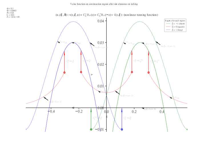
Figure 1: Relations between value functions $v(z,\xi,n),\xi=\{-1,0,1\}$ before and after the switching ($n=1\to 0$)

In this chart, each value function $v(z,\xi,1),\xi=\{-1,0,1\}$ over the continuation region is shown transitioning to $v(z,\hat{\xi},0)=\hat{v}(z,\hat{\xi}),\hat{\xi}=\{-1,0,1\}$ through regime switching from $\xi$ to $\hat{\xi}\in\mathcal{A}{}(\xi)$. This geometric-analytic relationship corresponds to the smooth pasting conditions—i.e., $C^{1}$-class continuity conditions connecting the functions before and after switching—at the connection represented by equation (89) on ${\mathcal{S}}_{n}^{\xi}$ on the condition of equations (93) and (94).

The figure is color-coded according to the three regimes. The value function for $\xi=0,n=0$ coincides with the horizontal axis and is thus not visible. Vertical arrows indicate the points at which switching occurs, and the length of each upward vector corresponds to the transaction cost.

According to the definition of the value function, it includes the expected cost from the current point onward, but past realized costs are excluded at the moment the event passes. Therefore, transaction costs are embedded in the value function as expectations just before switching, but once paid, they are removed as past events, resulting in an instantaneous upward jump in the value function equal to the transaction cost.

For example, the central red curve in Figure 1 represents the value function in the continuation region ${\mathcal{C}}_{1}^{0}$ for $\xi=0,n=1$. At the boundaries of this region, switching occurs to $\hat{\xi}=-1$ (green) on the right, or $\hat{\xi}=1$ (blue) on the left, transitioning to the continuation region ${\mathcal{C}}_{0}^{\hat{\xi}}=$ for $n=0$. Note that $v(z,\hat{\xi},0)=\hat{v}(z,\hat{\xi}),\;\hat{\xi}\in\mathbb{I}$ (defined on equation (85)) is defined over the entire real line as its continuation region.

The conditions for switching follow the procedures given in Theorem 3.2:

1. According to the boundary condition in equations (93) and (94), the curve $v(z,\xi,1)$ shifted upward by $K$ coincides with and is tangent to the corresponding curve $v(z,\hat{\xi},0)$ at the switching point (i.e., satisfies a $\mathcal{C}^{1}$-class condition).

2. According to equation (95), the upward-shifted curve $v(z,\xi,1)+K$ does not fall below any other subordinate value function $v(z,\hat{\xi},n-1)$ for all $\hat{\xi}\in\mathcal{A}{}(\xi)$.

These conditions are confirmed to hold for each of the three disjoint continuation regions ${\mathcal{C}}_{n}^{\xi\{\beta_{1}\}},{\mathcal{C}}_{n}^{\xi\{\beta_{2}\}},{\mathcal{C}}_{n}^{\xi\{\beta_{3}\}}$ comprising ${\mathcal{C}}_{n}^{\xi}$ with $\xi=0,n=1$. Similar confirmations can be made for all other regimes $\xi=\pm 1,n=1$.

Thus, the procedure for constructing $v(z,\xi,1),\xi\in\mathbb{I}$ from the known $v(z,\xi,0)=\hat{v}(z,\xi)$ is verified. Since $v(z,\xi,0)$ is given, the recursive procedure to obtain the value function for any $n\geq 0$ is also confirmed.

In this way, using the switching relation in equations (93) and (94), the complete value function graph—including values in switching regions—over the continuation region is presented in Figure 2.

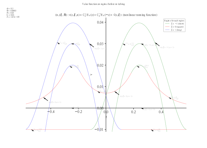
Figure 2: Value functions $v(z,\xi,n),\xi=\{-1,0,1\},n=0,1$

By repeating this procedure, the value function can be computed for any $n\geq 0$. As an example, the results up to $n=5$ are illustrated in Figure 3.

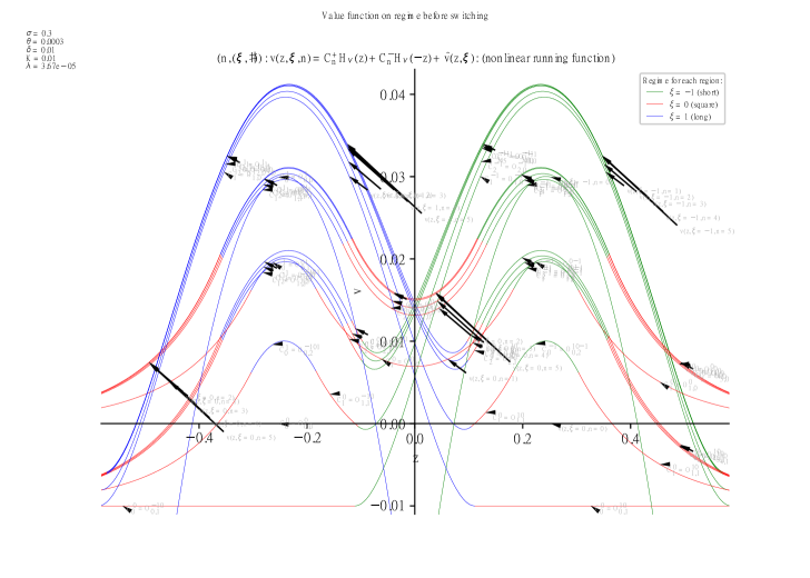
Figure 3: Value function $v(z,\xi,n),\xi=\{-1,0,1\},n=0,1,\cdots,5$

All the calculations to solve the viscosity solutions to the variational inequalities are done by Python programs with many special package libraries of Python. We have not used any numerical solvers, but only plot analytical functions analytically solved by PDEs with special function packages of Python. Below, Table 1 lists the standard and external Python libraries used in the analysis.

Package Name	Purpose	Usage in Analysis
math	Mathematical functions	Basic mathematical computations
numpy	Multi-dimensional arrays	Array and matrix operations
pandas	Data analysis	Data manipulation
matplotlib	Visualization	Chart and graph plotting
scipy	Special functions	Calling special functions
sqlite3	Database	Managing a database of optimal solutions
logging	Debugging	Managing output of debug information
portion	Interval arithmetic	Set operations over continuation regions

Table 1: Main Python standard and external packages used in the analysis

6 Conclusion

In this paper, we have presented a novel approach to solving a variational inequality arising in an infinite-horizon optimal switching problem with simultaneous multiple switchings. Building upon the uniqueness result of the viscosity solution shown in [Suzuki(2021)], we have demonstrated that, under appropriate assumptions, the viscosity solution can be explicitly constructed as a series of piecewise classical solutions. The key contribution lies in the establishment of necessary and sufficient smooth pasting conditions, which ensure that the concatenated classical solutions indeed satisfy the viscosity solution framework over the entire domain.

We proposed a practical algorithm for identifying all free boundary subproblems associated with the continuation and switching regions, and showed that this enables us to compute the complete value function recursively for any given number of remaining switches. The algorithm was applied to a pair-trading model based on an Ornstein–Uhlenbeck process. By solving each component analytically using special functions, we obtained a complete and explicit representation of the value functions without relying on numerical solvers.

The results not only provide a theoretical foundation for understanding the structure of the viscosity solution in such optimal switching problems but also offer a computationally feasible method for implementation in practice. The algorithmic framework and explicit formulas derived in this study can potentially be extended to more complex regime-switching models or multi-dimensional cases.

Future research may consider relaxing some of the assumptions, incorporating stochastic volatility, or applying the method to problems in energy economics, real options, and inventory control, where regime-switching behavior and transaction costs are inherent features.

References

- [Crandall et al.(1992)Crandall, Ishii & Lions] Crandall, M., Ishii, H., & Lions, P.-L. (1992). User’s guide to viscosity solutions of second order partial differential equations. Appeared in bulletin of the American mathematical society, 27, 1–67.
- [Fleming & Soner(1993)] Fleming, W. H., & Soner, H. M. (1993). Controlled Markov Processes and Viscosity Solutions. Springer-Verlag, New York.
- [Guo & Zhang(2005)] Guo, X., & Zhang, Q. (2005). Optimal selling rules in a regime switching model. IEEE transactions on automatic control, 50, 1450–1455.
- [Pemy & Zhang(2006)] Pemy, M., & Zhang, Q. (2006). Optimal stock liquidation in a regime switching model with finite time horizon. Journal of Mathematical Analysis and Applications, 321, 537–552.
- [Pham(2009)] Pham, H. (2009). Continuous-time Stochastic Control and Optimization with Financial Applications (Stochastic Modelling and Applied Probability). Springer-Verlag.
- [Pham & Vath(2007)] Pham, H., & Vath, V. L. (2007). Explicit solution to an optimal switching problem in the two-regimes case. SIAM J. Cont. Optim., 46, 395–426.
- [Pham et al.(2009)Pham, Vath & Zhou] Pham, H., Vath, V. L., & Zhou, X. Y. (2009). Optimal switching over multiple regimes. SIAM J. Cont. Optim., 48, 2217–2253.
- [Suzuki(2016)] Suzuki, K. (2016). Optimal switching strategy of a mean-reverting asset over multiple regimes. Automatica, 67, 33–45.
- [Suzuki(2018)] Suzuki, K. (2018). Optimal pair-trading strategy over long/short/square positions–empirical study. Quantitative Finance, 18, 97–119.
- [Suzuki(2021)] Suzuki, K. (2021). Infinite horizon optimal switching regions for pair-trading strategy with quadratic risk aversion considering simultaneous multiple switching: a viscosity solution approach. Mathematics of Operations Research, 46, 336–360.
- [Zervos(2003)] Zervos, M. (2003). A problem of sequential entry and exit decisions combined with discretionary stopping. SIAM Journal on Control and Optimization, 42, 397–421.
- [Zhang & Zhang(2008)] Zhang, H., & Zhang, Q. (2008). Trading a mean-reverting asset: Buy low and sell high. Automatica, 44, 1511–1518.