Don’t Reach for the Stars:
Rethinking Topology for Resilient Federated Learning

Abstract

Federated learning (FL) enables collaborative model training across distributed clients while preserving data privacy by keeping data local. Traditional FL approaches rely on a centralized, star-shaped topology, where a central server aggregates model updates from clients. However, this architecture introduces several limitations, including a single point of failure, limited personalization, and poor robustness to distribution shifts or vulnerability to malfunctioning clients. Moreover, update selection in centralized FL often relies on low-level parameter differences, which can be unreliable when client data is not independent and identically distributed, and offer clients little control. In this work, we propose a decentralized, peer-to-peer (P2P) FL framework. It leverages the flexibility of the P2P topology to enable each client to identify and aggregate a personalized set of trustworthy and beneficial updates. This framework is the Local Inference Guided Aggregation for Heterogeneous Training Environments to Yield Enhancement Through Agreement and Regularization (LIGHTYEAR). Central to our method is an agreement score, computed on a local validation set, which quantifies the semantic alignment of incoming updates in the function space with respect to the client’s reference model. Each client uses this score to select a tailored subset of updates and performs aggregation with a regularization term that further stabilizes the training. Our empirical evaluation across two datasets shows that the proposed approach consistently outperforms both centralized baselines and existing P2P methods in terms of client-level performance, particularly under adversarial and heterogeneous conditions. The code is available at: https://github.com/MECLabTUDA/LIGHTYEAR

Introduction

In recent years, federated learning (FL) has emerged as a powerful approach for collaboratively training machine learning models across a network of distributed clients, without requiring the exchange of raw data (McMahan et al. 2017). This paradigm has grown in popularity due to its natural fit for privacy- sensitive applications such as healthcare (Taiello et al. 2024; Ali et al. 2022), mobile personalization, and finance. FL was initially proposed in a centralized star-shaped topology, where a central server coordinates the training process (McMahan et al. 2017). While this approach is conceptually simple and effective for homogeneous settings, it struggles under real-world constraints. As research advanced and the scope of applications widened, significant challenges in the original architecture became apparent (Zhao et al. 2018). In FL, each client benefits most not from collaboration with the entire federation, but from a select subset of clients whose updates are best aligned with its own learning objectives (Chen, Li, and Shen 2024). These optimal subsets differ from one client to another, as an update that is useful for one may be irrelevant, or even harmful, for another client.

Figure 1: Arrow colors indicate the alignment quality of updates with the rest of the federation (green: well-aligned, yellow/red: misaligned). In centralized FL, all client updates are aggregated at the server regardless of their compatibility, which can degrade performance under heterogeneity. In contrast, P2P FL enables client-side aggregation, allowing each client to select only the most compatible updates.

This structure naturally arises due to two key factors. First, data heterogeneity is pervasive in real-world FL deployments. Clients often operate on non-independent and identically distributed (non-IID) data, which reflects unique user behaviors, sensing conditions, or hardware configurations, leading to non-exchangeability of data samples across clients (Zhu et al. 2021; Islam et al. 2024). As a result, the utility of a given update is not uniform across the federation. Aggregating updates from poorly aligned clients may degrade performance rather than improve it. Centralized FL, which aggregates updates from all clients into a single global model, overlooks the heterogeneity among client data distributions. This often results in suboptimal performance for individual clients (Li et al. 2019), introducing a systemic prediction error inherently tied to the centralized star-shaped topology.

Second, client reliability is inherently variable, and malfunctioning clients can introduce corrupted updates into the system. Such issues may arise from faulty sensors, broken data pipelines, or malicious attacks like model poisoning (Konstantin, Fuchs, and Mukhopadhyay 2024). In centralized FL, the server is responsible for filtering out such malfunctioning updates, typically through anomaly detection mechanisms that operate on model parameters or gradients (Blanchard et al. 2017; Sattler et al. 2020; Xu et al. 2022; Pillutla, Kakade, and Harchaoui 2022; Muñoz-González, Co, and Lupu 2019). However, these updates are often poor proxies for actual model behavior, since there is no consistent correlation between distances in parameter space and distances in function space (Benjamin, Rolnick, and Kording 2018). Crucially, the central server lacks access to local data (Liu, Xu, and Wang 2022) and cannot directly assess the predictive impact of client updates, making it impossible to evaluate their semantic compatibility or effectiveness. This limitation forces all clients to accept globally aggregated models that may be influenced by harmful or misaligned updates. Another systemic risk in centralized FL is the single point of failure at the central server (Qammar et al. 2023). A compromised or faulty central server can disrupt the training process, compromise the performance of all participating clients, and potentially expose sensitive information about their local training data (Zhang et al. 2024). This centralization bottleneck is not just a security risk, it also limits scalability and resilience (Sabuhi, Musilek, and Bezemer 2024; Gabrielli, Pica, and Tolomei 2023). These limitations highlight a fundamental mismatch between centralized FL architectures and the realities of heterogeneous and unreliable environments.

To address this, there is growing momentum toward decentralized, peer-to-peer (P2P) training architectures in FL (Gabrielli, Pica, and Tolomei 2023; Warnat-Herresthal et al. 2021). By moving away from a centralized star topology, these systems eliminate the central server and enable clients to exchange updates directly. This shift unlocks new opportunities for personalization, robustness, and autonomy. Rather than passively accepting a consensus global model, each client can now actively curate its own trusted subset of updates, referred to as its aggregation set, by selecting updates that align with its local objectives and data characteristics, as illustrated in Figure 1. In such decentralized settings, clients are empowered to perform local evaluation of incoming updates, using a private validation dataset, to assess their relevance and quality. This enables selective aggregation, where only semantically compatible and performance-improving updates are integrated into the aggregated model. As a result, decentralized FL emerges as a principled and practical solution for building personalized and robust models in heterogeneous settings.

We introduce the Local Inference Guided Aggregation for Heterogeneous Training Environments to Yield Enhancement Through Agreement and Regularization (LIGHTYEAR). This novel P2P FL framework is designed to select a personalized aggregation set for each client. Our approach begins with a formal characterization of the systemic prediction error that models experience on unseen target domains, accounting for both the violation of exchangeability between source and target domains and the impact of model malfunctions. To personalize the aggregation set for each client, LIGHTYEAR selects a subset of updates based on their estimated prediction error relative to the client’s target domain. Since clients lack access to other clients’ data distributions or training behaviors, we propose a novel agreement score that estimates the prediction error by measuring the alignment of an update with the client’s local data distribution in the function space. This score leverages the structural advantages of the P2P topology. Finally, we aggregate the selected models using a regularization term to mitigate the adverse effects of client drift in heterogeneous environments. As a result, LIGHTYEAR enables client-specific model aggregation while offering fine-grained control over the selection of updates. This enhances robustness against malfunctioning or irrelevant updates and leads to a reduction in systemic prediction error. Our findings demonstrate that P2P topologies offer superior robustness and personalization compared to centralized federated learning.

Our main contributions are as follows:

• We propose LIGHTYEAR, a framework that combines the agreement score for update selection and a regularized aggregation rule to enable robust and personalized model training in P2P FL.

• We introduce the agreement score, a novel metric that measures semantic alignment between client updates and the local model by estimating the prediction error on the target domain. This score is used to select the personalized set of updates for aggregation.

• We propose a regularized aggregation rule, which includes a round-dependent regularization term that controls the influence of updates over time, mitigating the effects of client drift in heterogeneous environments.

Related Work

To address prediction errors in FL, two main research directions have emerged: Robust FL focuses on mitigating the impact of malfunctioning clients and personalized FL, which tackles errors caused by distribution shifts across clients.

Robust Federated Learning

Malfunctioning clients pose a significant threat to FL by submitting harmful updates, whether due to adversarial intent or technical faults, that degrade the performance of the aggregated model when incorporated into the global update (Zhang et al. 2022; Konstantin, Fuchs, and Mukhopadhyay 2024). To mitigate the impact of such corrupted contributions, a variety of robust aggregation methods have been proposed. Originally introduced for centralized FL, these methods are typically performed at the server level, where no access to client-side data or reference performance metrics is available (Zhang et al. 2024). As a result, these approaches rely solely on distance-based measures computed over model parameters or gradients to assess the similarity between updates. Clients whose updates deviate significantly from the majority are either down-weighted during aggregation (Pillutla, Kakade, and Harchaoui 2022; Cao et al. 2020; Mhamdi, Guerraoui, and Rouault 2018) or excluded entirely (Blanchard et al. 2017; Sattler et al. 2020; Yin et al. 2018). With the growing interest in decentralized FL, robust aggregation methods have been adapted accordingly. In this setting, robustness must be ensured at the client level, and distance-based mechanisms are employed locally to evaluate incoming updates (Fang et al. 2024; He, Karimireddy, and Jaggi 2022).

Personalized Federated Learning

To address the limitations of the naive FedAvg approach in heterogeneous settings, where clients operate on non-IID data, personalized federated learning (pFL) was introduced to better adapt the global models to local client requirements. Rather than relying solely on a single shared model, pFL methods aim to tailor the learned representations to each client’s domain. Ditto (Li et al. 2021) extends this concept by maintaining two separate models per client: one global model for participation in communication rounds, and one personalized model for local inference, with training guided by a regularization term that encourages consistency between the two. FedALA (Zhang et al. 2023) introduces an additional local aggregation step, where each client combines the global model and its locally trained model using a weighted average, thereby adapting the global knowledge more flexibly to the local context.

Problem Statement

We consider a decentralized FL setting in which a set of clients $P=\{1,\ldots,P\}$ collaborate to learn a model. The network is structured as a P2P topology, where each client communicates directly with the other clients. Formally, for each client $i\in P$, let $\mathcal{N}(i)\subseteq P\setminus\{i\}$ denote the set of neighboring clients from whom it receives model updates $\{h_{j}\}_{j\in\mathcal{N}(i)}$. The client then aggregates these models with its own to update its parameters. A central challenge in this setting is that client $i$ has no information about the training data, optimization procedure, or reliability of its neighbors’ model updates $\{h_{j}\}_{j\in\mathcal{N}(i)}$. Consequently, it cannot determine a priori which of the updates will be beneficial or detrimental to its local objective. The naive aggregation of all received models,

$$h_{i}^{\text{new}}\leftarrow\text{Aggregate}\left(\{h_{j}\}_{j\in\mathcal{N}(i)}\cup\{h_{i}\}\right),$$

may introduce harmful biases. In particular, blindly aggregating all updates can degrade model performance in the following ways:

• Malicious clients may submit adversarial or poisoned updates $h_{j}^{\text{adv}}$ with the intent of corrupting the learning process.

• Unreliable clients may unintentionally produce corrupted updates $h_{j}^{\text{faulty}}$, e.g., due to defective data pipelines, incorrect labels, or faulty image acquisition.

• Non-exchangeability across clients: Even in benign scenarios, updates from clients trained on data distributions $\mathcal{D}_{j}$ significantly different from the client’s own distribution $\mathcal{D}_{i}$ may lead to performance degradation when aggregated (Zhao et al. 2018).

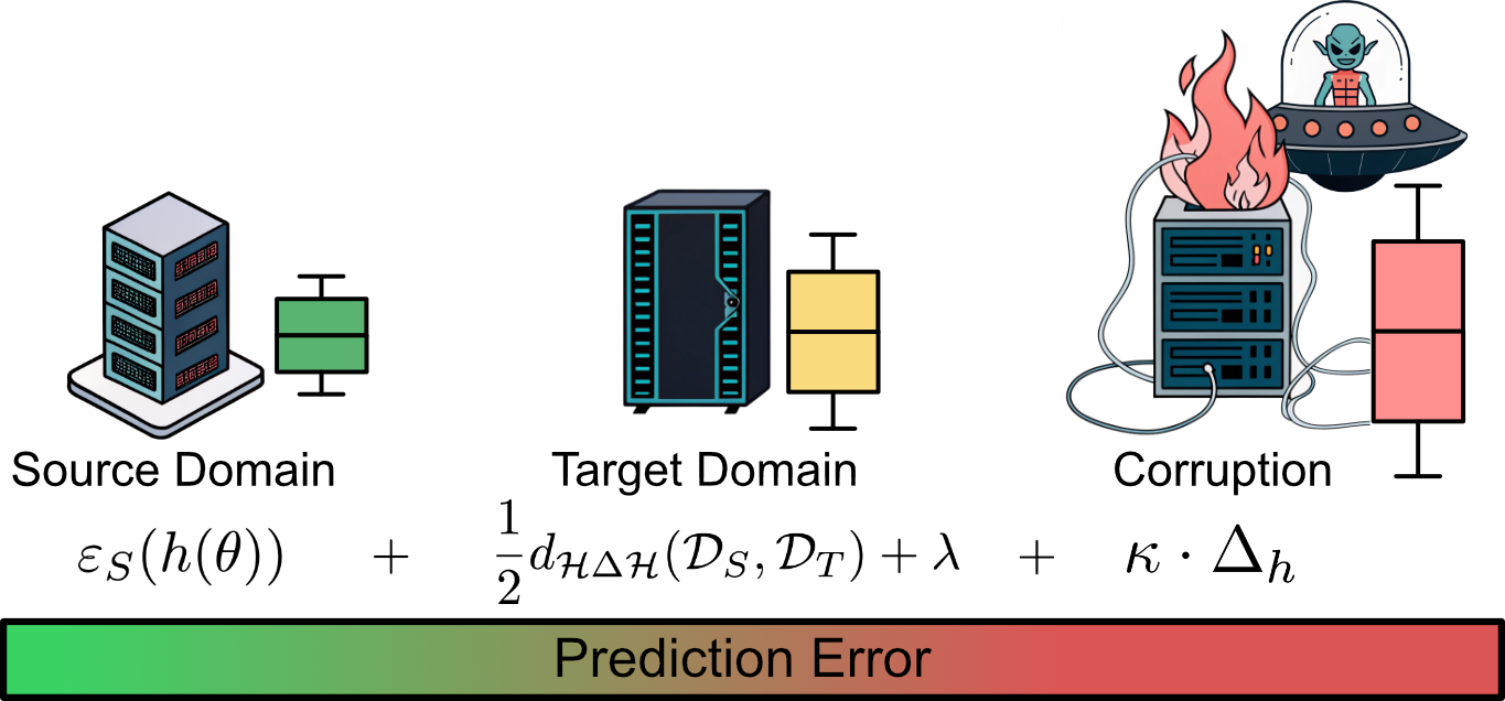
Figure 2: Illustration of the decomposition of the prediction error. The boxplot displays the error across the instances, with color indicating the magnitude of the error (green: low error, red: high error).

In general, model updates from such clients often exhibit structural divergence from the models trained on locally aligned data. Let $\varepsilon_{i}(h)$ denote the prediction error of model $h$ on client $i$’s distribution $\mathcal{D}_{i}$. Our goal is to identify a personalized aggregation set $\mathcal{S}_{i}\subseteq\mathcal{N}(i)$ of client updates such that:

$h_{i}^{\text{new}}\leftarrow\text{Aggregate}\left(\{h_{j}\}_{j\in\mathcal{S}_{i}}\cup\{h_{i}\}\right),$ where $\varepsilon_{i}(h_{i}^{\text{new}})\text{ is minimized}$. Thus, the fundamental problem is:

Given a set of client updates $\{h_{j}\}_{j\in\mathcal{N}(i)}$ and no access to their underlying data distributions or training errors, determine an optimal aggregation subset $\mathcal{S}_{i}\subseteq\mathcal{N}(i)$ that maximizes local performance on $\mathcal{D}_{i}$. This requires a reliable indicator for distributional similarity or alignment between updates and the local data of client $i$, which is the core methodological focus of our work.

Methodology

In the following, we begin by describing the prediction error a model incurs on a target distribution. This formulation accounts for both the violation of exchangeability between the source and target data distributions and the potential corruption of the model’s parameters due to malfunctions. We then highlight that P2P topologies offer a unique opportunity to approximate this error in a decentralized manner, in contrast to traditional star-shaped topologies. Finally, we introduce a novel agreement-based method that enables each client to select a custom aggregation set, thereby improving robustness and enhancing performance on the target distribution.

Exchangeability in Federated Learning

To consider the second case of disadvantageous clients, we must examine the concept of exchangeability, which plays a crucial role in the effectiveness of model aggregation. In statistical learning theory, a dataset $\{Z_{i}\}_{i=1}^{n}$ is said to be exchangeable if its joint distribution is invariant under permutations. Formally, a sequence $Z_{1},\ldots,Z_{n}$ is exchangeable if for any permutation $\pi$ of $\{1,\ldots,n\}$, the joint distribution satisfies:

$$P(Z_{1},\ldots,Z_{n})=P(Z_{\pi(1)},\ldots,Z_{\pi(n)}).$$ (1)

This condition generalizes the IID assumption and underpins the validity of many theoretical guarantees in machine learning, such as those provided by conformal prediction and generalization bounds.

In the context of FL, however, the assumption of data exchangeability across clients is often violated. Each client $i\in P$ may possess data drawn from a distinct underlying distribution $\mathcal{D}_{i}$, reflecting variability in user behavior, local environments, or sensing conditions. That is, while traditional learning assumes all data points $x_{i}\sim\mathcal{D}$, FL encounters the more general scenario where:

$$x_{i}\sim\mathcal{D}_{i},\quad\text{for }x_{i}\in\text{client }i.$$

As such, the global dataset is no longer exchangeable, and assumptions relying on this property break down.

Empirical and theoretical studies have shown that when clients violate exchangeability, such as by training on non-overlapping label distributions or domain-shifted data, the aggregated global model can suffer significant degradation in performance, particularly on the target distribution of interest (Lu et al. 2023). This issue is exacerbated by the fact that clients’ local data distributions are not observable, either due to privacy constraints or system limitations. Consequently, we lack the information necessary to directly assess how well each client’s model update aligns with the target task.

Malfunctioning Clients

While violations of exchangeability across client updates arise from training on heterogeneous data distributions, leading to prediction errors as discussed above, malfunctioning clients represent a more extreme case of misalignment. In contrast to clients optimized for a specific data distribution, malfunctioning clients are generally misaligned with all data distributions within the federation. In our work, we consider three distinct types of client malfunctions. Two of these represent untargeted model poisoning attacks, namely, the Additive-Noise Attack (ANA) and the Sign-Flipping Attack (SFA), which are widely studied attacks in the FL literature (Konstantin, Fuchs, and Mukhopadhyay 2024; Li et al. 2020; Alebouyeh and Bidgoly 2024).

In the ANA setting, a client perturbs its model parameters by adding Gaussian noise before broadcasting, i.e., the transmitted update becomes

$$\tilde{\theta}=\theta+\varepsilon,\quad\varepsilon\sim\mathcal{N}(0,\sigma^{2}I),$$ (2)

where $\theta$ is the locally trained model and $\varepsilon$ is the noise vector.

In the SFA setting, the client multiplies the entire update by a negative constant, effectively reversing the optimization direction:

$$\tilde{\theta}=-\alpha\cdot\theta,\quad\alpha>0$$ (3)

In addition to adversarial behaviors, we simulate a malfunction indicative of technical failures, such as broken data pipelines or failed local training. In this scenario, the client submits a model update consisting of randomly initialized weights, entirely bypassing the optimization process and severing any connection to meaningful training.

Error Decomposition

As previously described, prediction errors may arise due to either malfunctions or the violation of exchangeability between the source and target distributions. In other words, if $x_{i}\sim\mathcal{D}_{S}$ during training and $x_{j}\sim\mathcal{D}_{T}$ during testing with $\mathcal{D}_{S}\neq\mathcal{D}_{T}$, then the exchangeability assumption is violated. The latter can be understood as natural shifts inherent to distributional differences, while malfunctions represent unnatural shifts introduced through adversarial or unexpected faulty behavior. Therefore, the overall prediction error of a corrupted model $h(\tilde{\theta})$ on a target distribution $T$ can be expressed as the combination of these two sources of error:

$$\varepsilon(h(\tilde{\theta}))=\varepsilon_{T}(h(\theta))+\varepsilon_{\mathcal{M}}(h(\tilde{\theta}))$$ (4)

where:

• $\varepsilon_{T}(h(\theta))$ is the error of model $h$ with parameters $\theta$ on the target domain

• $\varepsilon_{\mathcal{M}}(h({\tilde{\theta}}))$is the error of model $h$ due to corrupted parameters $\tilde{\theta}$

This concept is visualized in Figure 2. To quantify the impact of this shift, the domain adaptation framework developed by Ben-David et al.(Ben-David et al. 2010) provides a theoretical upper bound on the expected target domain error of a model $h\in\mathcal{H}$, trained on a source distribution $\mathcal{D}_{S}$, and evaluated on a target distribution $\mathcal{D}_{T}$. The bound is given as:

$$\varepsilon_{T}(h(\theta))\leq\varepsilon_{S}(h(\theta))+\frac{1}{2}d_{\mathcal{H}\Delta\mathcal{H}}(\mathcal{D}_{S},\mathcal{D}_{T})+\lambda,$$ (5)

where:

• $\varepsilon_{T}(h(\theta))$ is the expected error of $h$ with parameters $\theta$ on the target distribution $\mathcal{D}_{T}$,

• $\varepsilon_{S}(h(\theta))$ is the expected error of $h$ with parameters $\theta$ on the source distribution $\mathcal{D}_{S}$,

• $d_{\mathcal{H}\Delta\mathcal{H}}(\mathcal{D}_{S},\mathcal{D}_{T})$ is the $\mathcal{H}\Delta\mathcal{H}$-divergence between the source and target distributions, and

• $\lambda$ is the combined error of the ideal model on both domains, defined as:

  $$\lambda=\min_{h(\theta)\in\mathcal{H}}\left[\varepsilon_{S}(h(\theta))+\varepsilon_{T}(h(\theta))\right]$$ (6)

This bound demonstrates that the error on the target domain is influenced not only by the model’s performance on the source domain but also by the divergence between the source and target distributions.

On the other hand, the unnatural shift causing a prediction error can be described as the deviation introduced by malfunctioning model parameters, rather than by inherent differences in data distributions. This type of shift disrupts the expected behavior of the model and leads to additional prediction error.

$$\varepsilon_{\mathcal{M}}(h(\tilde{\theta}))=\kappa\cdot\Delta_{h}$$ (7)

where:

• $\kappa$ is the level of corruption

• $\Delta_{h}$is the sensitivity to corruption of model $h$

Thus, the overall error of the corrupted model can be described as:

$$\varepsilon_{T}(h(\tilde{\theta}))\leq\underbrace{\varepsilon_{S}(h(\theta))+\frac{1}{2}d_{\mathcal{H}\Delta\mathcal{H}}(D_{S},D_{T})+\lambda}_{\text{exchangeability}}+\underbrace{\kappa\cdot\Delta_{h}}_{\text{corruption}}$$ (8)

To assess the sensitivity $\Delta_{h}$ of the models used in this work, we added an ablation study to the supplementary material that investigates how the prediction error changes with the level of corruption $\kappa$.

Approximation by Agreement

To improve robustness in FL, we ideally want to incorporate only those client updates into aggregation that are well aligned with the desired target distribution. This means selecting an aggregation set consisting of client updates yielding a low prediction error, as previously described. However, since the target distribution may vary across clients, the optimal aggregation set becomes client-specific. Unlike traditional star-shaped topologies, P2P topologies allow each client to construct its own personalized aggregation set. Unfortunately, clients do not have access to the local data distributions of the other clients, nor can they observe their prediction errors during training, both of which are essential for accurately estimating the prediction error on the target distribution. What is available to client $i$ are: (1) its own locally trained model $h_{i}$, used as reference and representative of the local distribution, trained on data from $\mathcal{D}_{i}$, and (2) a local validation dataset $V_{i}=\{(x_{k},y_{k})\}_{k=1}^{n}$ drawn from a distribution $\mathcal{D}_{\text{val}}\approx\mathcal{D}_{i}$. Therefore, we need to reconsider the problem from another point of view. As previously described, a malfunctioning model will exhibit a higher prediction error on the target distribution compared to a model that was specifically optimized for it. This increased error manifests as a behavioral divergence between the two models when making predictions on the target domain. In particular, the corrupted model $h^{m}$ will tend to disagree with the optimal model $h^{*}$, which was trained to minimize error on that specific distribution. This disagreement indicates the presence of a prediction error apart from the irreducible error inherent to the task. Therefore, we can describe the relation as $\varepsilon_{T}(h(\tilde{\theta}))\sim\delta_{\mathcal{T}}(h(\theta^{*}),h(\tilde{\theta}))$, where $\delta_{\mathcal{T}}(h(\theta^{*}),h(\tilde{\theta}))$ denotes a disagreement in prediction of the two models on a target domain $\mathcal{T}$.

From this perspective, our goal is to identify a personalized aggregation set for each client, consisting only of client updates that exhibit strong agreement with the client’s local reference model. Let $h_{i}:=h(\theta_{i})$ and $h_{j}:=h(\theta_{j})$ denote the models of client $i$ and client $j$, respectively, where $\theta_{i}$ and $\theta_{j}$ are their respective parameter vectors. For clarity, we denote the composite agreement score as $A_{ij}:=A(h_{i},h_{j};V_{i})$, where the components $A^{\text{Acc}}_{ij}$, $A^{\text{ECE}}_{ij}$, and $A^{\text{Sharp}}_{ij}$ respectively denote accuracy agreement, calibration agreement, and sharpness agreement—each computed over client $i$’s local validation set $V_{i}$. The agreement score is defined as follows:

$$A_{ij} =\frac{1}{3}(A_{ij}^{\text{Acc}}+A_{ij}^{\text{ECE}}+A_{ij}^{\text{Sharp}}),$$ (9)

$$A_{ij}^{\text{Acc}} =\frac{1}{|V_{i}|}\sum_{(x_{i},y_{i})\in V_{i}}\left(\mathbf{1}[h_{i}(x_{i})=y_{i}]-\mathbf{1}[h_{j}(x_{i})=y_{i}]\right),$$ (10)

$$A_{ij}^{\text{ECE}} =1-|\text{ECE}(h_{i};V_{i})-\text{ECE}(h_{j};V_{i})|,$$ (11)

$$A_{ij}^{\text{Sharp}} =1-\frac{1}{|V_{i}|}\sum_{x\in V_{i}}|H(p_{i}(x))-H(p_{j}(x))|,$$ (12)

where:

• $\text{ECE}(h;V)$ is the expected calibration error of model $h$ on dataset $V$

• $p_{i}(x)\text{ is defined as softmax}(h_{i}(x))$

• $H(p(x))=-\sum_{k=1}^{K}p_{k}(x)\log p_{k}(x)$ is the entropy (sharpness) of the predictive distribution

Update selection Based on the agreement score defined in the previous section, we leverage a filtering mechanism that enables each client to selectively aggregate only those updates whose predictions are sufficiently aligned with its own reference model. We introduce a selection threshold $\tau\in\mathbb{R}$ and define the aggregation set $S_{i}$ for client $i$ as:

$$S_{i}=\{\theta_{j}\in\mathcal{N}(i)\mid A(h_{i},h_{j};V_{i})\geq\tau\}.$$ (13)

which contains only those peer models that are considered sufficiently similar to the local model in terms of predictive behavior on the validation data. Since the agreement score is computed as an empirical average over the validation set, the thresholding mechanism corresponds to a form of marginal coverage in the conformal prediction sense (Romano, Sesia, and Candes 2020), meaning we retain those updates that show high average agreement with the local model on marginally sampled inputs from $\mathcal{D}_{i}$.

Aggregation

After selecting the aggregation set, the chosen updates are aggregated to obtain the new model. To enhance robustness, we introduce a regulation parameter into the aggregation process, as shown in Eq 14.

$$\bar{\theta_{i}}^{(t+1)}=\bar{\theta_{i}}^{(t)}+\gamma^{t}\cdot\frac{1}{|\mathcal{S}_{i}|}\sum_{j\in\mathcal{S}_{i}}\left(\theta_{j}-\bar{\theta_{i}}^{(t)}\right)$$ (14)

This parameter is dependent on the training round and can be interpreted as a decay of change, reflecting our observation of a gradual performance decline after a certain number of training rounds. By incorporating this decay, the aggregation becomes more stable and resilient to fluctuations. We have included the corresponding ablation study in the appendix to support our findings. Notably, setting the regulation parameter to 1 reduces the method to the standard FedAvg over the updates from the selected aggregation set.

Datasets

To evaluate the effectiveness of our proposed decentralized federated learning method, we conducted experiments on two diverse datasets, each chosen to reflect realistic non-IID client distributions. These datasets span different domains to ensure that the evaluation is robust across various data modalities and levels of heterogeneity. Each client holds an individual training, validation and test set, created through a random train-validation-test split of their local data.

FEMNIST(Caldas et al. 2018) consists of $28\times 28$ grayscale images of handwritten digits and characters spanning 62 classes. The dataset is partitioned by writer identity, assigning each client a unique, non-overlapping subset of writers. This results in distinct local data distributions per client, reflecting realistic heterogeneity. We consider a total of 8 clients, with the specific data partitions for each client detailed in the appendix. The clients leverage a CNN with two layers for this task.

Camelyon17-WILDS(Bandi et al. 2018) consists of $98\times 98$ tissue slide patches used for a binary tumor classification task. The dataset includes samples from patients across five hospitals, which naturally divide into two distinct groups based on the image acquisition protocols employed. Specifically, two of the hospitals used a different acquisition protocol than the remaining three, leading to a clear distribution shift between the two groups. In our setup, each client corresponds to one hospital, resulting in five clients in total. Each client independently trains a DenseNet121 model(Huang et al. 2017) on its local data.

The detailed training setup and dataset composition are provided in the supplementary. Our experiments were executed using NVIDIA A100 GPUs, and we implemented all experiments using the NVIDIA FLARE FL framework(Roth et al. 2022).

Experiments

In the following experiments, we consider three different types of malfunctions: ANAs, SFAs and clients who submit random updates. For each experiment, we incrementally increase the number of malfunctioning clients, meaning that the number of malfunctioning clients grows per run. We compare LIGHTYEAR against FedAvg (McMahan et al. 2017) and seven baseline methods for robust aggregation: AFA (Muñoz-González, Co, and Lupu 2019), ASMR (Konstantin, Fuchs, and Mukhopadhyay 2024), CFL (Sattler et al. 2020), Ditto (Li et al. 2021), Krum (Blanchard et al. 2017), BALANCE (Fang et al. 2024), and SCCLIP(Yang and Ghaderi 2024). While BALANCE and SCCLIP are also P2P methods, the others represent baselines from FL with a star-shaped topology. The performance of each method is evaluated based on the average accuracy on each client’s test set. The experiments focus on three key scenarios: (1) evaluating the resilience of each method against the three types of malfunctions individually, (2) assessing the resilience based on topology as the number of malfunctioning clients increases, and (3) testing the resilience in a dynamic and highly unpredictable environment, where malfunctioning clients randomly select one of the three malfunctions each round. This dynamic scenario aims to simulate conditions that are more representative of real-world situations. For LIGHTYEAR, we set the hyperparameter $\gamma$ to 0.95 in both cases. The decision threshold $\tau$ was set to 0.75 for FEMNIST and 0.6 for Camelyon17, reflecting the higher distributional diversity and smaller number of clients in the latter. More detailed results for all experiments are provided in the supplementary material.

Results

The results demonstrate a significant performance improvement of LIGHTYEAR over all compared baselines. As shown in Figure 3, the aggregated overall performance is reported for an increasing number of malfunctioning clients, averaged over all runs and clients.

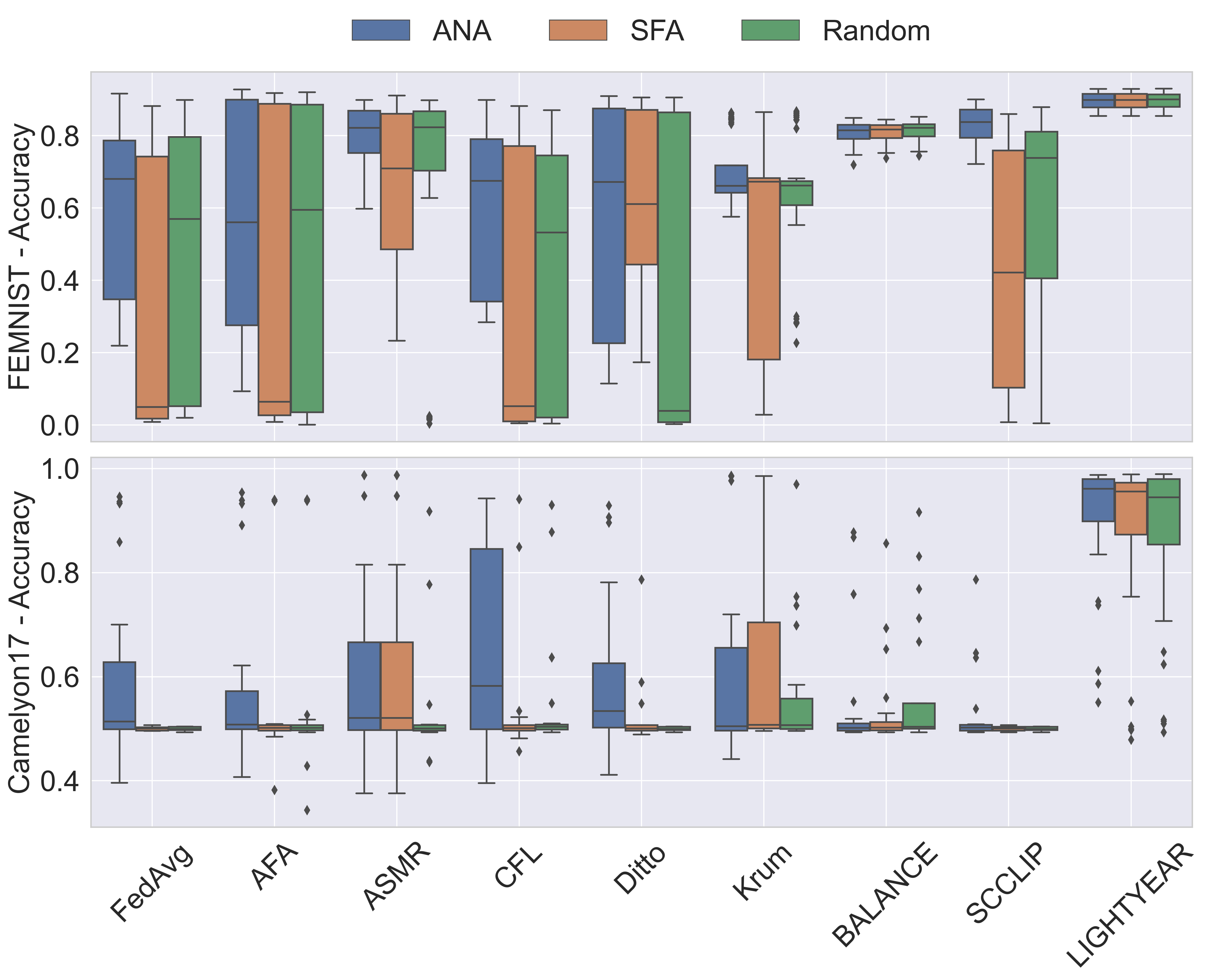
Figure 3: illustrates the robustness of each method under three types of client malfunctions. We evaluate performance by progressively increasing the number of malfunctioning clients, ranging from 1-7 for FEMNIST and from 1-4 for Camelyon17. The reported accuracy represents the average accuracy across all clients and all experimental runs.

Notably, LIGHTYEAR is the only method that maintains stability across all cases on both datasets. This is particularly evident on the Camelyon17 dataset, where no other method was able to achieve a reliable state under the given conditions. Consequently, the other methods failed to be resilient against the errors described in Eq 8. For additional insights, we provide more detailed results in the appendix, where the detailed performance across all experiments is listed in tables. Figure 4 illustrates the resilience of each method against the three discussed malfunctions, broken down by topology and increasing number of malfunctioning clients.

Figure 4: compares the resilience of both topologies and LIGHTYEAR to three types of client malfunctions. The x-axis indicates the number of malfunctioning clients, while the y-axis shows the average accuracy across all clients.

While P2P methods show significant stability in FEMNIST against ANAs, only LIGHTYEAR fully leverages the potential of the P2P topology by remaining robust across all considered cases. Finally, Figure 5 showcases a more dynamic scenario, where the robustness against an increasing number of malfunctioning clients is tested, with each malfunctioning client randomly selecting one of the three malfunction types per round. As observed, LIGHTYEAR continues to demonstrate superior stability even in this more dynamic setting.

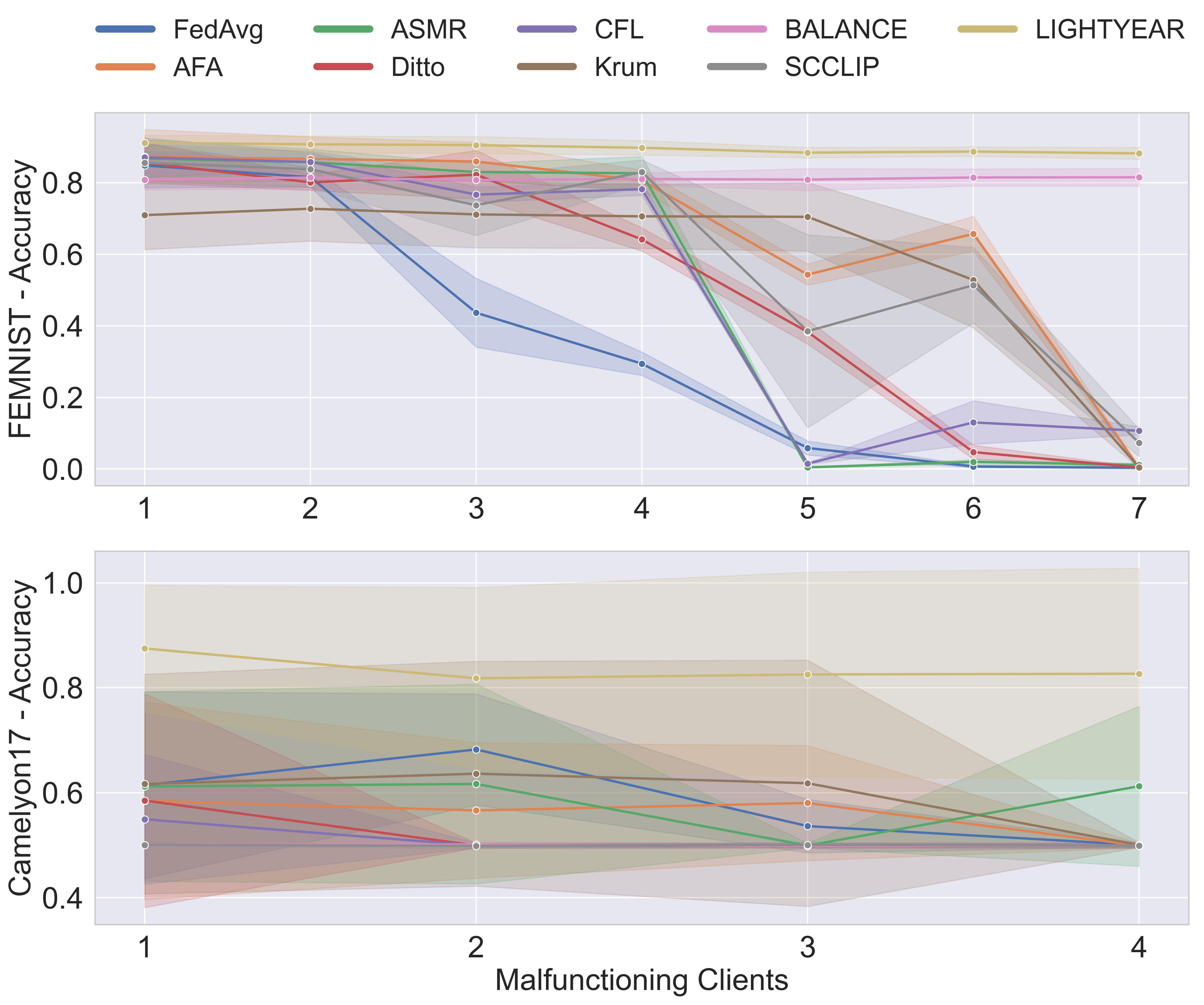
Figure 5: illustrates the resilience of each method to dynamically changing client malfunctions. The x-axis indicates the number of malfunctioning clients; in this setting, each malfunctioning client randomly selects one of the three malfunction types in every round. The y-axis shows the average accuracy across all clients, along with the standard deviation.

Ablation

As an ablation study, we showcase the impact of the regularization term $\gamma$ on the aggregation process in FL. To isolate the effect of the regularization term, we compare the training process of FedAvg with a version of FedAvg that includes the regularization term. Note that setting $\gamma=1$ corresponds to standard FedAvg. The accuracy, as illustrated in Figure 6, is evaluated on each client’s validation set and is averaged over all clients. Notably, on the Camelyon17 Dataset, where the distribution shift between clients is more pronounced, the impact of the regularization term is particularly evident, highlighting its effectiveness in mitigating the negative effects of heterogeneity and improving model robustness.

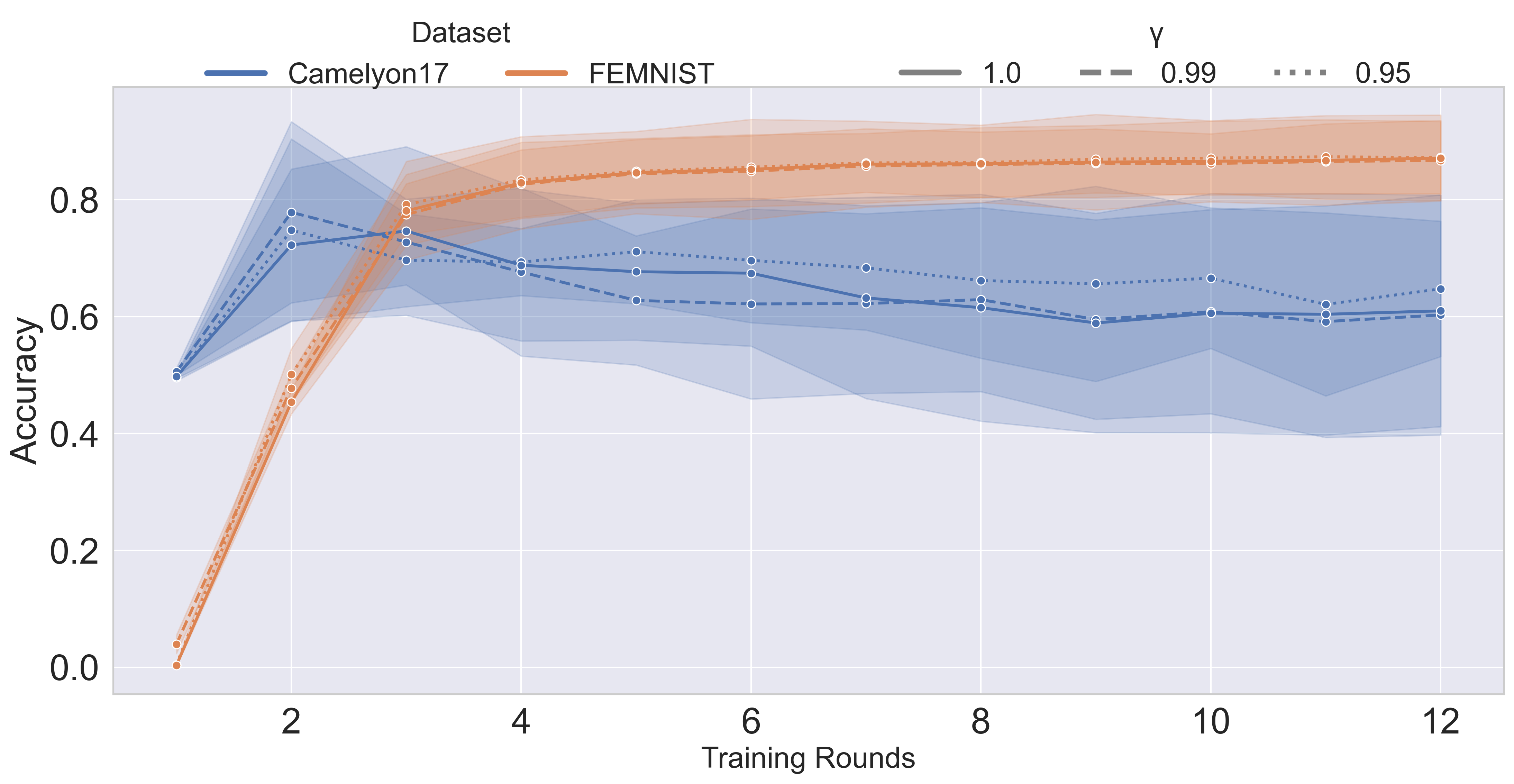
Figure 6: Accuracy and standard deviation averaged across all clients, measured on each client’s validation set.

Conclusion

In this work, we explored the P2P FL setting and addressed the challenge that the optimal aggregation set varies across clients, as only a subset of clients provides valuable updates for any given client. Identifying this subset is essential to maximizing the benefits of FL, especially in the presence of diverse, potentially unreliable, or misaligned participants. While star-shaped topologies offer global coordination, they are inherently limited in their ability to address the personalized needs of individual clients. We proposed LIGHTYEAR, a novel method tailored for the P2P topology. It introduces a client-specific selection mechanism that enables each client to construct a personalized aggregation set by estimating the prediction error on its local data distribution. This estimation is based on an agreement score that measures the alignment of received updates with a reference model in the function space. Additionally, LIGHTYEAR employs a regularized aggregation strategy to stabilize training and improve robustness. Our experimental results illustrate that LIGHTYEAR improves performance over both traditional centralized federated learning methods and state-of-the-art decentralized alternatives. This paper contends that we should stop reaching for the stars and instead shift towards decentralized architectures that offer greater reliability and personalization in ever-changing training conditions.

Appendix A Supplementary Material

In this section, we provide an overview of the hardware and software requirements needed to reproduce our experiments. We detail the dataset construction process for each client in our FL setup, ensuring reproducibility of the data splits and assignments. Additionally, we outline the model architectures used in our experiments, including all relevant hyperparameters.

Hard- and Software Requirements

Our implementation is based on NVIDIA FLARE, as described in the main paper. The required software configuration includes Python 3.10.17, CUDA 12.2, and PyTorch 2.7.0+cu126. We also used a nightly build of FLARE 2.6.1. All remaining dependencies are listed in the requirements.txt file provided in our codebase. Experiments were conducted on a SLURM-managed cluster using NVIDIA A100 GPUs with 40GB memory. For the centralized FL experiments, we used a total of three GPUs, while for the decentralized setup, we assigned one GPU per client. This allocation was primarily dictated by the FLARE-specific implementation requirements rather than the computational demands of the models.

Dataset Construction

As mentioned in the main text, each client holds a unique training, validation, and test set. For the Camelyon17 dataset, data from five different hospitals is used, with each client assigned data from one specific hospital. Figure 7 showcases the clients’ data distributions by representative examples. Within each client, a random train/validation/test split is performed. We generated a CSV file, called p2pfl_metadata.csv, that records the assignment of all samples to clients and their respective splits. This file is included in the datasets directory of our codebase.

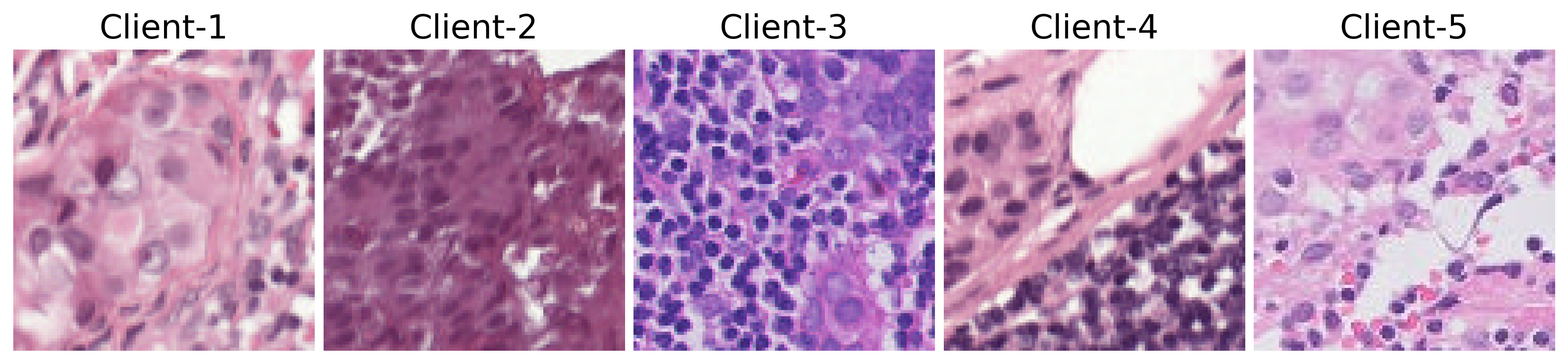
Figure 7: Sample images from each client, illustrating distinct differences in their data distributions. These variations highlight the heterogeneity across clients, which contributes to prediction errors on target domains as described in Eq 5 of the main paper, and underline the challenges of training in federated settings.

For the second dataset, FEMNIST, we used the dataset structure provided by the LEAF (https://github.com/TalwalkarLab/leaf) repository. In this setting, each client receives a distinct subset of data corresponding to a unique set of writers. Similar to the Camelyon17 setup, a random train/validation/test split is performed on each client’s data. Our preprocessing scripts for generating these subsets and splits are also included in the datasets directory of our codebase.

Training Details

To complement the description of our training routines provided in the main paper, we present the detailed hyperparameters for our experimental setup in Table 1. Additionally, our codebase includes the full implementation of these training routines, ensuring that all experiments are fully reproducible.

	FEMNIST	Camelyon17
Loss Function	Cross Entropy	Cross Entropy
Optimizer	Adam	SGD
Learning Rate	1e-3	1e-3
Weight Decay	1e-4	5e-4
Momentum	-	0.9
Batchsize	32	32
Rounds	12	12
Local Epochs	1	1

Table 1: The Hyperparameters for the training routines of the experiments.

Appendix B Model Sensitivity

To investigate the sensitivity of the models used in our study to corrupted updates, we conducted an ablation study using the ANA. In the main paper, we employed two model architectures: a DenseNet121 for the Camelyon17 dataset, chosen due to its prevalence on the official leaderboard, and a lightweight CNN with two convolutional layers for the FEMNIST dataset, which has shown strong performance on this task. To evaluate how these models react to corrupted updates, we applied ANA as defined in Equation 7 of the main paper. In our implementation, noise is injected into the updates using a scaling factor $s$, as described in Equation 15, allowing us to vary the corruption severity from very light to heavy flexibly. This tunable corruption is an advantage over SFA, which inherently applies only strong corruption. For our ablation, we applied different scaling factors and varied the number of malfunctioning clients, ranging from 1 to 3 for FEMNIST, and from 1 to 2 for Camelyon17. We monitored how the corruption affected the learning dynamics by evaluating each client’s local validation accuracy at every training round. The mean validation accuracy across all clients per round is reported in Figure 8 for FEMNIST and Figure 9 for Camelyon17.

Figure 8: Training performance on FEMNIST under varying levels of corruption. Each plot corresponds to a different number of malfunctioning clients, indicated in parentheses in the y-axis label. Results show the average validation accuracy across all clients at each training round.

Figure 9: Training performance on Camelyon17 under varying levels of corruption. Each plot corresponds to a different number of malfunctioning clients, indicated in parentheses in the y-axis label. Results show the average validation accuracy across all clients at each training round.

$$\tilde{\theta}_{k}=\theta_{k}+\left(\epsilon_{k}\cdot\frac{s}{100}\cdot\theta_{k}\right),\quad\text{where}\quad\epsilon_{k}\sim\mathcal{N}(0,I)$$ (15)

Our ablation study reveals that the model trained on the FEMNIST dataset exhibits strong robustness to noise and is therefore less sensitive to corruption. We evaluated this sensitivity using four different noise scaling factors, as detailed in Figure 1. The results indicate that even scaling factors around 50 do not destabilize the training process. However, when scaling reaches around 120, the training begins to show instability, even with only a single malfunctioning client. At a scaling factor of approximately 150, we observe significant performance degradation, particularly when three clients are malfunctioning. In contrast, the model trained on the Camelyon17 dataset is much more sensitive to noise. As a result, we evaluated this setting using substantially smaller scaling factors. Even at a scaling of 1.5, the training becomes noticeably destabilized. It is worth noting that training on Camelyon17 is inherently less stable and more challenging due to the high degree of client heterogeneity. This instability is also reflected in the main paper’s ablation study and motivated our introduction of the regularized aggregation approach. In our final experiments, we used a scaling factor of 120.5 for FEMNIST and 1.5 for Camelyon17. While these settings do not lead to the most extreme performance drops, they effectively destabilize training and negatively impact performance, striking a balance between subtle corruption and the more aggressive, rapidly diverging effect of SFAs.

Appendix C Experimental Results

In this section, we provide a detailed breakdown of the results presented in the main paper. For each dataset and malfunction, a dedicated table is included. These tables report the average accuracy across all clients, along with the corresponding standard deviation. All values are expressed as percentages for consistency and clarity.

Table 2: This table reports the results for ANAs on FEMNIST. Average accuracy (%) $\pm$ std of each method under increasing number of malfunctioning clients.

FEMNIST – ANA
Number of Malfunctioning Clients
Method	1	2	3	4	5	6	7
FedAvg	86.0 $\pm$ 8.3	84.7 $\pm$ 7.3	75.0 $\pm$ 5.8	59.4 $\pm$ 5.5	68.1 $\pm$ 8.0	25.0 $\pm$ 1.2	31.2 $\pm$ 4.9
AFA	87.2 $\pm$ 6.7	87.3 $\pm$ 6.5	87.0 $\pm$ 5.1	54.3 $\pm$ 3.9	52.7 $\pm$ 4.0	16.0 $\pm$ 3.9	25.0 $\pm$ 3.0
ASMR	86.1 $\pm$ 4.8	85.5 $\pm$ 2.5	85.3 $\pm$ 2.1	81.5 $\pm$ 2.0	78.2 $\pm$ 5.3	73.6 $\pm$ 8.0	70.6 $\pm$ 8.5
CFL	86.7 $\pm$ 5.8	86.0 $\pm$ 4.0	85.5 $\pm$ 2.6	13.5 $\pm$ 1.2	66.2 $\pm$ 3.6	36.2 $\pm$ 3.2	21.2 $\pm$ 1.6
Ditto	84.1 $\pm$ 8.6	76.0 $\pm$ 4.7	80.3 $\pm$ 7.7	68.4 $\pm$ 1.9	32.5 $\pm$ 2.0	31.2 $\pm$ 2.3	36.7 $\pm$ 4.1
Krum	68.6 $\pm$ 9.4	68.5 $\pm$ 9.2	70.0 $\pm$ 9.1	69.2 $\pm$ 9.2	70.5 $\pm$ 8.7	70.5 $\pm$ 9.2	70.1 $\pm$ 9.1
BALANCE	80.2 $\pm$ 2.8	81.3 $\pm$ 2.3	81.3 $\pm$ 1.6	81.9 $\pm$ 2.6	82.1 $\pm$ 2.2	79.0 $\pm$ 2.8	80.2 $\pm$ 3.4
SCCLIP	86.0 $\pm$ 3.6	85.1 $\pm$ 3.7	85.9 $\pm$ 3.7	84.0 $\pm$ 3.4	80.4 $\pm$ 4.8	80.5 $\pm$ 3.1	80.5 $\pm$ 3.3
LIGHTYEAR	90.6 $\pm$ 2.2	90.6 $\pm$ 1.8	90.7 $\pm$ 2.0	90.3 $\pm$ 2.3	89.0 $\pm$ 1.7	88.2 $\pm$ 1.4	88.1 $\pm$ 1.6

Table 3: This table reports the results for SFAs on FEMNIST. Average accuracy (%) $\pm$ std of each method under increasing number of malfunctioning clients.

FEMNIST – SFA
Number of Malfunctioning Clients
Method	1	2	3	4	5	6	7
FedAvg	83.6 $\pm$ 5.4	76.6 $\pm$ 2.4	21.4 $\pm$ 5.7	1.5 $\pm$ 0.3	1.3 $\pm$ 0.3	3.6 $\pm$ 0.4	4.5 $\pm$ 1.5
AFA	86.9 $\pm$ 7.1	87.0 $\pm$ 6.1	86.0 $\pm$ 4.2	2.6 $\pm$ 0.3	6.4 $\pm$ 0.9	2.9 $\pm$ 0.3	1.6 $\pm$ 0.3
ASMR	87.2 $\pm$ 4.6	86.8 $\pm$ 3.4	84.9 $\pm$ 1.7	73.0 $\pm$ 6.3	58.8 $\pm$ 4.6	42.5 $\pm$ 10.5	36.6 $\pm$ 2.9
CFL	86.9 $\pm$ 4.8	85.9 $\pm$ 3.4	85.2 $\pm$ 3.2	25.6 $\pm$ 4.4	51.3 $\pm$ 12.5	55.3 $\pm$ 1.1	43.4 $\pm$ 10.0
Ditto	84.3 $\pm$ 4.2	77.6 $\pm$ 1.9	7.7 $\pm$ 1.0	5.1 $\pm$ 0.5	1.4 $\pm$ 0.3	0.8 $\pm$ 0.2	0.9 $\pm$ 0.1
Krum	71.4 $\pm$ 8.8	71.5 $\pm$ 8.2	70.9 $\pm$ 9.0	71.4 $\pm$ 8.2	71.0 $\pm$ 8.7	3.5 $\pm$ 0.5	15.5 $\pm$ 3.2
BALANCE	81.0 $\pm$ 2.5	80.0 $\pm$ 2.3	81.3 $\pm$ 2.4	81.1 $\pm$ 2.0	81.4 $\pm$ 2.3	80.9 $\pm$ 3.1	81.2 $\pm$ 3.0
SCCLIP	83.8 $\pm$ 2.6	78.9 $\pm$ 3.3	67.6 $\pm$ 8.2	42.1 $\pm$ 16.1	16.7 $\pm$ 5.2	6.6 $\pm$ 5.0	2.4 $\pm$ 1.0
LIGHTYEAR	90.1 $\pm$ 2.1	90.5 $\pm$ 2.2	89.8 $\pm$ 2.6	89.6 $\pm$ 1.5	88.9 $\pm$ 1.6	88.4 $\pm$ 1.1	88.5 $\pm$ 2.0

Table 4: This table reports the results for the Random malfunction on FEMNIST. Average accuracy (%) $\pm$ std of each method under increasing number of malfunctioning clients.

FEMNIST – Random
Number of Malfunctioning Clients
Method	1	2	3	4	5	6	7
FedAvg	85.6 $\pm$ 6.5	77.2 $\pm$ 3.0	79.6 $\pm$ 5.4	57.2 $\pm$ 3.8	10.0 $\pm$ 0.9	2.4 $\pm$ 0.4	4.2 $\pm$ 1.2
AFA	87.0 $\pm$ 7.1	86.7 $\pm$ 6.3	86.0 $\pm$ 4.2	60.0 $\pm$ 3.8	5.0 $\pm$ 1.5	4.1 $\pm$ 1.6	0.4 $\pm$ 0.3
ASMR	86.8 $\pm$ 3.9	86.0 $\pm$ 3.5	85.2 $\pm$ 1.8	82.5 $\pm$ 2.3	77.5 $\pm$ 5.4	72.4 $\pm$ 8.6	1.6 $\pm$ 0.7
CFL	86.7 $\pm$ 4.9	85.8 $\pm$ 2.7	85.2 $\pm$ 2.2	3.9 $\pm$ 1.1	0.4 $\pm$ 0.2	0.6 $\pm$ 0.2	3.0 $\pm$ 0.1
Ditto	83.1 $\pm$ 5.0	81.3 $\pm$ 5.7	71.8 $\pm$ 2.9	53.1 $\pm$ 2.6	2.3 $\pm$ 0.6	1.7 $\pm$ 0.7	1.6 $\pm$ 0.7
Krum	70.5 $\pm$ 8.8	70.8 $\pm$ 8.7	70.1 $\pm$ 8.9	69.5 $\pm$ 9.6	70.7 $\pm$ 9.0	66.2 $\pm$ 9.4	35.4 $\pm$ 13.3
BALANCE	81.7 $\pm$ 2.8	80.4 $\pm$ 2.7	81.3 $\pm$ 2.3	81.4 $\pm$ 2.5	80.8 $\pm$ 2.5	81.2 $\pm$ 3.3	82.0 $\pm$ 1.6
SCCLIP	84.6 $\pm$ 2.6	83.6 $\pm$ 3.5	77.8 $\pm$ 4.2	74.9 $\pm$ 3.3	65.5 $\pm$ 6.0	31.7 $\pm$ 13.9	4.8 $\pm$ 2.2
LIGHTYEAR	90.8 $\pm$ 2.1	90.9 $\pm$ 2.2	90.0 $\pm$ 2.1	90.1 $\pm$ 1.9	89.1 $\pm$ 1.4	88.5 $\pm$ 1.1	89.6 $\pm$ 1.7

Table 5: This table reports the results for the dynamically changing malfunction on FEMNIST. Average accuracy (%) $\pm$ std of each method under increasing number of malfunctioning clients.

FEMNIST – Dynamic Malfunctions
Number of Malfunctioning Clients
Method	1	2	3	4	5	6	7
FedAvg	84.9 $\pm$ 5.8	81.6 $\pm$ 2.6	43.7 $\pm$ 9.0	29.4 $\pm$ 3.1	5.9 $\pm$ 1.8	0.7 $\pm$ 0.3	0.3 $\pm$ 0.2
AFA	87.3 $\pm$ 7.2	86.7 $\pm$ 5.8	86.0 $\pm$ 5.0	80.6 $\pm$ 2.7	54.4 $\pm$ 2.7	65.7 $\pm$ 4.5	0.4 $\pm$ 0.2
ASMR	86.8 $\pm$ 4.9	85.8 $\pm$ 3.4	83.0 $\pm$ 2.3	82.7 $\pm$ 4.4	0.5 $\pm$ 0.1	2.0 $\pm$ 0.6	1.1 $\pm$ 0.4
CFL	87.1 $\pm$ 5.1	85.8 $\pm$ 2.4	76.7 $\pm$ 2.0	78.2 $\pm$ 1.6	1.5$\pm$ 0.2	13.0 $\pm$ 5.7	10.7 $\pm$ 1.0
Ditto	85.6 $\pm$ 5.2	80.1 $\pm$ 2.0	82.3 $\pm$ 6.3	64.2 $\pm$ 3.0	38.3 $\pm$ 3.2	4.7 $\pm$ 1.8	0.4 $\pm$ 0.2
Krum	71.0 $\pm$ 9.0	72.8 $\pm$ 8.5	71.2 $\pm$ 8.7	70.6 $\pm$ 8.4	70.5 $\pm$ 8.9	52.8 $\pm$ 12.5	0.4 $\pm$ 0.2
BALANCE	80.7 $\pm$ 2.6	81.5 $\pm$ 3.0	80.8 $\pm$ 2.6	81.8 $\pm$ 1.6	80.9 $\pm$ 2.9	81.5 $\pm$ 2.2	81.6 $\pm$ 2.3
SCCLIP	85.6 $\pm$ 4.8	83.8 $\pm$ 4.8	73.7 $\pm$ 7.9	83.0 $\pm$ 3.2	38.5 $\pm$ 2.5	51.4 $\pm$ 9.9	7.3 $\pm$ 3.6
LIGHTYEAR	91.2 $\pm$ 2.0	90.8 $\pm$ 2.2	90.5 $\pm$ 2.2	89.8 $\pm$ 1.9	88.4 $\pm$ 1.4	88.7 $\pm$ 1.2	88.2 $\pm$ 1.6

Table 6: This table reports the results for ANAs on Camelyon17. Average accuracy (%) $\pm$ std of each method under increasing number of malfunctioning clients.

Camelyon17 – ANA
Number of Malfunctioning Clients
Method	1	2	3	4
FedAvg	58.8 $\pm$ 14.2	61.6 $\pm$ 18.2	59.5 $\pm$ 17.6	58.3 $\pm$ 18.5
AFA	59.8 $\pm$ 19.0	58.5 $\pm$ 17.5	59.0 $\pm$ 15.1	56.6 $\pm$ 19.1
ASMR	54.3 $\pm$ 10.3	61.5 $\pm$ 17.3	61.3 $\pm$ 14.9	60.6 $\pm$ 20.0
CFL	58.3 $\pm$ 16.8	58.1 $\pm$ 18.2	69.4 $\pm$ 16.9	73.8 $\pm$ 18.8
Ditto	64.1 $\pm$ 15.4	64.7 $\pm$ 16.1	59.3 $\pm$ 17.0	51.4 $\pm$ 0.5
Krum	80.2 $\pm$ 0.4	77.5 $\pm$ 0.5	74.0 $\pm$ 0.6	70.1 $\pm$ 0.7
BALANCE	50.2 $\pm$ 0.4	51.5 $\pm$ 2.0	57.5 $\pm$ 15.9	62.3 $\pm$ 15.9
SCCLIP	58.8 $\pm$ 11.3	50.0 $\pm$ 0.4	50.8 $\pm$ 1.6	52.7 $\pm$ 5.5
LIGHTYEAR	90.9 $\pm$ 14.9	84.8 $\pm$ 15.7	94.7 $\pm$ 0.4	93.5 $\pm$ 0.5

Table 7: This table reports the results for SFAs on Camelyon17. Average accuracy (%) $\pm$ std of each method under increasing number of malfunctioning clients.

Camelyon17 – SFA
Number of Malfunctioning Clients
Method	1	2	3	4
FedAvg	50.1 $\pm$ 0.4	50.1 $\pm$ 0.4	50.1 $\pm$ 0.4	50.4 $\pm$ 0.4
AFA	56.6 $\pm$ 19.1	58.6 $\pm$ 17.7	50.1 $\pm$ 0.4	50.1 $\pm$ 0.4
ASMR	56.1 $\pm$ 17.9	60.6 $\pm$ 17.8	50.0 $\pm$ 0.4	50.1 $\pm$ 0.4
CFL	56.3 $\pm$ 14.4	59.5 $\pm$ 17.4	50.1 $\pm$ 0.4	50.1 $\pm$ 0.4
Ditto	58.3 $\pm$ 10.8	50.1 $\pm$ 0.4	50.1 $\pm$ 0.4	50.1 $\pm$ 0.4
Krum	80.2 $\pm$ 0.4	77.5 $\pm$ 0.5	74.0 $\pm$ 0.6	70.1 $\pm$ 0.7
BALANCE	55.3 $\pm$ 7.4	53.0 $\pm$ 6.2	57.5 $\pm$ 14.3	50.0 $\pm$ 0.4
SCCLIP	50.1 $\pm$ 0.4	50.1 $\pm$ 0.4	50.1 $\pm$ 0.4	50.1 $\pm$ 0.4
LIGHTYEAR	84.7 $\pm$ 17.6	81.2 $\pm$ 15.0	87.8 $\pm$ 19.0	94.2 $\pm$ 3.2

Table 8: This table reports the results for Random malfunction on Camelyon17. Average accuracy (%) $\pm$ std of each method under increasing number of malfunctioning clients.

Camelyon17 – Random
Number of Malfunctioning Clients
Method	1	2	3	4
FedAvg	50.4 $\pm$ 0.4	50.4 $\pm$ 0.4	50.4 $\pm$ 50.4	50.4 $\pm$ 0.4
AFA	57.5 $\pm$ 18.3	56.5 $\pm$ 20.0	50.0 $\pm$ 0.4	50.0 $\pm$ 0.4
ASMR	55.3 $\pm$ 11.8	57.1 $\pm$ 17.5	50.0 $\pm$ 0.4	50.1 $\pm$ 0.4
CFL	60.0 $\pm$ 16.6	60.5 $\pm$ 14.6	50.0 $\pm$ 0.4	50.0 $\pm$ 0.4
Ditto	50.0 $\pm$ 0.4	50.0 $\pm$ 0.4	50.4 $\pm$ 0.4	50.4 $\pm$ 0.4
Krum	80.2 $\pm$ 0.4	77.5 $\pm$ 0.5	74.0 $\pm$ 0.6	70.1 $\pm$ 0.7
BALANCE	53.5 $\pm$ 6.6	62.4 $\pm$ 16.8	62.0 $\pm$ 14.9	50.2 $\pm$ 0.4
SCCLIP	50.0 $\pm$ 0.4	50.0 $\pm$ 0.4	50.0 $\pm$ 0.4	50.0 $\pm$ 0.4
LIGHTYEAR	82.4 $\pm$ 18.3	80.9 $\pm$ 15.4	87.4 $\pm$ 19.2	91.6 $\pm$ 0.7

Table 9: This table reports the results for the dynamically changing malfunction on Camelyon17. Average accuracy (%) $\pm$ std of each method under increasing number of malfunctioning clients.

Camelyon17 – Dynamic Malfunctions
Number of Malfunctioning Clients
Method	1	2	3	4
FedAvg	61.5 $\pm$ 15.9	68.2 $\pm$ 9.5	53.6 $\pm$ 4.5	50.1 $\pm$ 0.4
AFA	58.5 $\pm$ 16.8	56.6 $\pm$ 11.5	58.0 $\pm$ 9.8	50.0 $\pm$ 0.4
ASMR	61.2 $\pm$ 16.1	61.7 $\pm$ 17.0	50.0 $\pm$ 0.6	61.3 $\pm$ 13.6
CFL	58.5 $\pm$ 18.2	50.0 $\pm$ 0.4	50.0 $\pm$ 0.4	50.0 $\pm$ 0.4
Ditto	55.0 $\pm$ 11.0	50.0 $\pm$ 0.4	50.0 $\pm$ 0.4	50.0 $\pm$ 0.4
Krum	61.7 $\pm$ 18.7	63.6 $\pm$ 19.2	61.8 $\pm$ 21.0	50.1 $\pm$ 0.4
BALANCE	50.1 $\pm$ 0.4	50.1 $\pm$ 0.4	50.0 $\pm$ 0.4	50.0 $\pm$ 0.4
SCCLIP	50.0 $\pm$ 0.4	50.1 $\pm$ 0.4	50.0 $\pm$ 0.4	50.0 $\pm$ 0.4
LIGHTYEAR	87.5 $\pm$ 10.8	81.8 $\pm$ 15.5	82.5 $\pm$ 17.4	82.7 $\pm$ 18.0

References

- Alebouyeh and Bidgoly (2024) Alebouyeh, Z.; and Bidgoly, A. J. 2024. Benchmarking robustness and privacy-preserving methods in federated learning. Future Generation Computer Systems, 155: 18–38.
- Ali et al. (2022) Ali, M.; Naeem, F.; Tariq, M.; and Kaddoum, G. 2022. Federated learning for privacy preservation in smart healthcare systems: A comprehensive survey. IEEE journal of biomedical and health informatics, 27(2): 778–789.
- Bandi et al. (2018) Bandi, P.; Geessink, O.; Manson, Q.; Van Dijk, M.; Balkenhol, M.; Hermsen, M.; Bejnordi, B. E.; Lee, B.; Paeng, K.; Zhong, A.; et al. 2018. From detection of individual metastases to classification of lymph node status at the patient level: the camelyon17 challenge. IEEE transactions on medical imaging, 38(2): 550–560.
- Ben-David et al. (2010) Ben-David, S.; Blitzer, J.; Crammer, K.; Kulesza, A.; Pereira, F.; and Vaughan, J. W. 2010. A theory of learning from different domains. Machine learning, 79: 151–175.
- Benjamin, Rolnick, and Kording (2018) Benjamin, A. S.; Rolnick, D.; and Kording, K. 2018. Measuring and regularizing networks in function space. arXiv preprint arXiv:1805.08289.
- Blanchard et al. (2017) Blanchard, P.; El Mhamdi, E. M.; Guerraoui, R.; and Stainer, J. 2017. Machine learning with adversaries: Byzantine tolerant gradient descent. Advances in neural information processing systems, 30.
- Caldas et al. (2018) Caldas, S.; Duddu, S. M. K.; Wu, P.; Li, T.; Konečnỳ, J.; McMahan, H. B.; Smith, V.; and Talwalkar, A. 2018. Leaf: A benchmark for federated settings. arXiv preprint arXiv:1812.01097.
- Cao et al. (2020) Cao, X.; Fang, M.; Liu, J.; and Gong, N. Z. 2020. Fltrust: Byzantine-robust federated learning via trust bootstrapping. arXiv preprint arXiv:2012.13995.
- Chen, Li, and Shen (2024) Chen, Z.; Li, J.; and Shen, C. 2024. Personalized federated learning with attention-based client selection. In ICASSP 2024-2024 IEEE International Conference on Acoustics, Speech and Signal Processing (ICASSP), 6930–6934. IEEE.
- Fang et al. (2024) Fang, M.; Zhang, Z.; Hairi; Khanduri, P.; Liu, J.; Lu, S.; Liu, Y.; and Gong, N. 2024. Byzantine-robust decentralized federated learning. In Proceedings of the 2024 on ACM SIGSAC Conference on Computer and Communications Security, 2874–2888.
- Gabrielli, Pica, and Tolomei (2023) Gabrielli, E.; Pica, G.; and Tolomei, G. 2023. A survey on decentralized federated learning. arXiv preprint arXiv:2308.04604.
- He, Karimireddy, and Jaggi (2022) He, L.; Karimireddy, S. P.; and Jaggi, M. 2022. Byzantine-robust decentralized learning via clippedgossip. arXiv preprint arXiv:2202.01545.
- Huang et al. (2017) Huang, G.; Liu, Z.; Van Der Maaten, L.; and Weinberger, K. Q. 2017. Densely connected convolutional networks. In Proceedings of the IEEE conference on computer vision and pattern recognition, 4700–4708.
- Islam et al. (2024) Islam, M. S.; Javaherian, S.; Xu, F.; Yuan, X.; Chen, L.; and Tzeng, N.-F. 2024. FedClust: Optimizing federated learning on non-IID data through weight-driven client clustering. In 2024 IEEE International Parallel and Distributed Processing Symposium Workshops (IPDPSW), 1184–1186. IEEE.
- Konstantin, Fuchs, and Mukhopadhyay (2024) Konstantin, M.; Fuchs, M.; and Mukhopadhyay, A. 2024. ASMR: Angular Support for Malfunctioning Client Resilience in Federated Learning. In Medical Imaging with Deep Learning, 754–767. PMLR.
- Li et al. (2020) Li, S.; Cheng, Y.; Wang, W.; Liu, Y.; and Chen, T. 2020. Learning to detect malicious clients for robust federated learning. arXiv preprint arXiv:2002.00211.
- Li et al. (2021) Li, T.; Hu, S.; Beirami, A.; and Smith, V. 2021. Ditto: Fair and robust federated learning through personalization. In International conference on machine learning, 6357–6368. PMLR.
- Li et al. (2019) Li, X.; Huang, K.; Yang, W.; Wang, S.; and Zhang, Z. 2019. On the convergence of fedavg on non-iid data. arXiv preprint arXiv:1907.02189.
- Liu, Xu, and Wang (2022) Liu, P.; Xu, X.; and Wang, W. 2022. Threats, attacks and defenses to federated learning: issues, taxonomy and perspectives. Cybersecurity, 5(1): 4.
- Lu et al. (2023) Lu, C.; Yu, Y.; Karimireddy, S. P.; Jordan, M.; and Raskar, R. 2023. Federated conformal predictors for distributed uncertainty quantification. In International Conference on Machine Learning, 22942–22964. PMLR.
- McMahan et al. (2017) McMahan, B.; Moore, E.; Ramage, D.; Hampson, S.; and y Arcas, B. A. 2017. Communication-efficient learning of deep networks from decentralized data. In Artificial intelligence and statistics, 1273–1282. PMLR.
- Mhamdi, Guerraoui, and Rouault (2018) Mhamdi, E. M. E.; Guerraoui, R.; and Rouault, S. 2018. The hidden vulnerability of distributed learning in byzantium. arXiv preprint arXiv:1802.07927.
- Muñoz-González, Co, and Lupu (2019) Muñoz-González, L.; Co, K. T.; and Lupu, E. C. 2019. Byzantine-robust federated machine learning through adaptive model averaging. arXiv preprint arXiv:1909.05125.
- Pillutla, Kakade, and Harchaoui (2022) Pillutla, K.; Kakade, S. M.; and Harchaoui, Z. 2022. Robust aggregation for federated learning. IEEE Transactions on Signal Processing, 70: 1142–1154.
- Qammar et al. (2023) Qammar, A.; Karim, A.; Ning, H.; and Ding, J. 2023. Securing federated learning with blockchain: a systematic literature review. Artificial Intelligence Review, 56(5): 3951–3985.
- Romano, Sesia, and Candes (2020) Romano, Y.; Sesia, M.; and Candes, E. 2020. Classification with valid and adaptive coverage. Advances in neural information processing systems, 33: 3581–3591.
- Roth et al. (2022) Roth, H. R.; Cheng, Y.; Wen, Y.; Yang, I.; Xu, Z.; Hsieh, Y.-T.; Kersten, K.; Harouni, A.; Zhao, C.; Lu, K.; et al. 2022. Nvidia flare: Federated learning from simulation to real-world. arXiv preprint arXiv:2210.13291.
- Sabuhi, Musilek, and Bezemer (2024) Sabuhi, M.; Musilek, P.; and Bezemer, C.-P. 2024. Micro-fl: A fault-tolerant scalable microservice-based platform for federated learning. Future Internet, 16(3): 70.
- Sattler et al. (2020) Sattler, F.; Müller, K.-R.; Wiegand, T.; and Samek, W. 2020. On the byzantine robustness of clustered federated learning. In ICASSP 2020-2020 IEEE International Conference on Acoustics, Speech and Signal Processing (ICASSP), 8861–8865. IEEE.
- Taiello et al. (2024) Taiello, R.; Cansiz, S.; Vesin, M.; Cremonesi, F.; Innocenti, L.; Önen, M.; and Lorenzi, M. 2024. Enhancing Privacy in Federated Learning: Secure Aggregation for Real-World Healthcare Applications. In International Conference on Medical Image Computing and Computer-Assisted Intervention, 204–214. Springer.
- Warnat-Herresthal et al. (2021) Warnat-Herresthal, S.; Schultze, H.; Shastry, K. L.; Manamohan, S.; Mukherjee, S.; Garg, V.; Sarveswara, R.; Händler, K.; Pickkers, P.; Aziz, N. A.; et al. 2021. Swarm learning for decentralized and confidential clinical machine learning. Nature, 594(7862): 265–270.
- Xu et al. (2022) Xu, J.; Huang, S.-L.; Song, L.; and Lan, T. 2022. Byzantine-robust federated learning through collaborative malicious gradient filtering. In 2022 IEEE 42nd International Conference on Distributed Computing Systems (ICDCS), 1223–1235. IEEE.
- Yang and Ghaderi (2024) Yang, C.; and Ghaderi, J. 2024. Byzantine-robust decentralized learning via remove-then-clip aggregation. In Proceedings of the AAAI Conference on Artificial Intelligence, volume 38, 21735–21743.
- Yin et al. (2018) Yin, D.; Chen, Y.; Kannan, R.; and Bartlett, P. 2018. Byzantine-robust distributed learning: Towards optimal statistical rates. In International conference on machine learning, 5650–5659. Pmlr.
- Zhang et al. (2024) Zhang, C.; Yang, S.; Mao, L.; and Ning, H. 2024. Anomaly detection and defense techniques in federated learning: a comprehensive review. Artificial Intelligence Review, 57(6): 150.
- Zhang et al. (2023) Zhang, J.; Hua, Y.; Wang, H.; Song, T.; Xue, Z.; Ma, R.; and Guan, H. 2023. Fedala: Adaptive local aggregation for personalized federated learning. In Proceedings of the AAAI conference on artificial intelligence, volume 37, 11237–11244.
- Zhang et al. (2022) Zhang, Z.; Cao, X.; Jia, J.; and Gong, N. Z. 2022. Fldetector: Defending federated learning against model poisoning attacks via detecting malicious clients. In Proceedings of the 28th ACM SIGKDD conference on knowledge discovery and data mining, 2545–2555.
- Zhao et al. (2018) Zhao, Y.; Li, M.; Lai, L.; Suda, N.; Civin, D.; and Chandra, V. 2018. Federated learning with non-iid data. arXiv preprint arXiv:1806.00582.
- Zhu et al. (2021) Zhu, H.; Xu, J.; Liu, S.; and Jin, Y. 2021. Federated learning on non-IID data: A survey. Neurocomputing, 465: 371–390.