mathx”17

*: All authors contributed equally to this paper and their names are listed in alphabetical order by last name.

1 Introduction

In the era of big data, privacy concerns have become a critical issue, especially when handling sensitive personal or confidential information. Major regulations such as the European Union’s General Data Protection Regulation (GDPR), the California Consumer Privacy Act (CCPA), and China’s Personal Information Protection Law (PIPL) reflect the global emphasis on data privacy. From a theoretical perspective, ensuring privacy is a key issue that underpins much of the current research. Differential privacy (DP) has emerged as a rigorous mathematical framework that provides quantifiable privacy guarantees. The concept was formally introduced by [1] using probabilistic models. DP ensures that the inclusion or exclusion of any single individual’s data does not significantly affect the outcome of any analysis, thereby protecting individual privacy. This property is particularly important in data-driven processes, where large datasets are used for statistical modeling, machine learning, and predictive analytics. The authors of [2] demonstrated that adding random noise from specific distributions, such as Laplace, normal, or binomial, can ensure differential privacy. The authors of [3] further provided a comprehensive overview of DP construction methods, detailing both algorithmic principles and practical implementations. Additionally, the authors of [4] conducted an information-theoretic analysis, establishing upper bounds for the min-entropy leakage of differentially private mechanisms. By introducing carefully calibrated noise, DP guarantees that outputs do not reveal sensitive information about any individual. As a result, DP has become increasingly relevant in fields such as healthcare, finance, and the social sciences, where privacy protection is critical.

In addition to privacy concerns, the distributed nature of modern datasets presents significant challenges for statistical learning. As data is often collected and stored across multiple nodes or devices, traditional centralized approaches to data analysis become impractical. Distributed learning algorithms are needed to efficiently process and analyze large-scale datasets while respecting privacy constraints. These algorithms must be able to handle heterogeneous data distributions, varying sample sizes, and communication limitations between nodes. In many real-world settings, data often exhibit heavy-tailed and skewed noise, along with outliers and heterogeneity. Quantile regression (QR) has emerged as a powerful tool in statistical modeling for enhancing robustness. Unlike traditional mean regression, which focuses on estimating the conditional mean, quantile regression provides a more comprehensive view of the relationship between variables by estimating different quantiles, making it particularly useful in the presence of outliers or heavy-tailed error distributions [5, 6]. However, the non-smooth nature of the quantile loss function poses computational challenges, especially in high-dimensional settings where the number of covariates can be very large. This complexity is further exacerbated in distributed environments, where constraints on multi-round communication and privacy requirements must be taken into account.

Existing literature has explored various aspects of differentially private statistical learning, including mean estimation [7, 8], linear regression [7, 9], and distributed learning [10, 11, 12, 13]. Another line of research has focused on developing efficient distributed algorithms for quantile regression, particularly in high-dimensional settings [14, 15]. However, these methods either do not incorporate differential privacy or do not address the challenges posed by heavy-tailed noise and heteroscedastic data. The investigation of robust estimation and inference techniques in a distributed and differentially private manner is particularly pressing.

In this paper, we first develop a privacy-preserving framework for distributed estimation and inference in high-dimensional sparse quantile regression, addressing three foundational questions:

• Q1: How to perform DP high-dimensional quantile regression with heavy-tailed noise and heteroscedastic data in the distributed setting?

• Q2: How does DP affect the statistical accuracy of high-dimensional distributed quantile regression in both estimation and inference?

• Q3: How should efficient DP estimation and inference be achieved with communication constraints under distributed learning?

1.1 Literature Review on differential privacy in Statistical Learning

In recent years, the integration of privacy-preserving techniques into traditional machine learning methods has become increasingly prevalent, driven by advances in artificial intelligence and the growing importance of data privacy [1, 3]. Since the seminal introduction of differential privacy by [1], a wide range of privacy-preserving mechanisms have been developed. Local differential privacy (LDP), also introduced in [16], enforces a stricter privacy guarantee by adding noise directly on the client side, thus eliminating the need for a trusted curator. More recently, Gaussian differential privacy (GDP) was proposed by [17], which characterizes privacy loss using a single parameter based on a unit-variance Gaussian distribution. This framework provides an intuitive and analytically tractable approach to quantifying privacy.

These privacy frameworks (DP, LDP, GDP) are now being actively integrated into diverse machine learning paradigms, where the unique characteristics of the learning task—such as data dimensionality (low vs. high) and system architecture (centralized vs. distributed)—significantly influence both the implementation of privacy mechanisms and their statistical/computational costs. We now review relevant work in these specific contexts.

Low-Dimensional Estimation with Differential Privacy. Balancing privacy protection and statistical accuracy remains a central challenge in differential privacy. In low-dimensional settings, the addition of noise to ensure privacy often leads to a loss in accuracy, a trade-off extensively studied in [18, 19, 20]. Recent advances have significantly improved DP frameworks for core statistical tasks. For mean estimation, the authors of [21] provided a unified hypothesis testing perspective under GDP, while robust DP-compatible estimators have been developed in [22], and [23] established person-level DP bounds. Covariance estimation has benefited from efficient clip-and-noise strategies [24]. In linear regression, DP variants include privatized F-tests [25] and ridge regression with confidence-preserving intervals [26]. Minimax-optimal estimators under LDP have been proposed by [27], and [28] established minimax lower bounds in the LDP setting. The authors of [29] connected robust M-estimators to DP via sensitivity-calibrated noise, showing asymptotic equivalence to non-private procedures, while [30] linked Huber’s contamination model to LDP, demonstrating that robust methods can often be efficiently privatized. Fundamental trade-offs, such as the bias–variance–privacy triad in mean estimation [31], highlight inherent limitations, though symmetry assumptions can sometimes enable unbiased estimation under approximate DP.

High-Dimensional Estimation and Inference with Differential Privacy. With the increasing demand for privacy-preserving techniques in high-dimensional sparse settings, the development of efficient sparse algorithms under differential privacy has become crucial. The authors of [32] introduced the “peeling” (Noisy Hard Thresholding) algorithm, which provides an efficient and practical approach for high-dimensional differentially private data analysis. This method has been widely adopted in the design of differentially private algorithms for high-dimensional problems, as seen in works such as [7, 33, 34]. However, as highlighted by [7], high-dimensional privacy protection inevitably incurs a “cost of privacy”—an increase in estimation error as model complexity grows. This privacy-utility trade-off has been studied in various contexts, including top-$k$ feature selection [35], sparse mean estimation [7], covariance estimation [36], sparse linear regression [37, 7, 9], and least absolute deviation regression [38]. More recently, [39] explored private learning in high-dimensional regimes where the dimension grows proportionally to the sample size.

Most existing research on differential privacy for high-dimensional data has focused on statistical estimation, often leveraging the iterative hard thresholding gradient-descent framework of [40]. In contrast, differentially private inference in high dimensions remains relatively underdeveloped. Notable recent advances include [34], who proposed inference procedures for high-dimensional linear regression—such as differentially private false discovery rate control—and [41], who developed DP nonparametric tests for generalized linear models and the Bradley–Terry–Luce model, establishing minimax separation rates. Nevertheless, key inference tasks in high-dimensional statistical learning remain open, and most existing work is still limited to linear models.

Distributed Statistical Learning with Differential Privacy. Despite these advances, the integration of differential privacy with a broad range of statistical methods in distributed environments remains relatively underexplored. In low-dimensional settings, The authors of [10] developed communication-efficient DP stochastic gradient descent algorithms, while [42] proposed a one-shot DP logistic regression method. The authors of [43] designed a communication-efficient protocol that operates without a trusted machine. For high-dimensional models, The authors of [44] investigated decentralized data ownership, and [8] introduced a multi-round DP gradient method for high-dimensional linear regression under heterogeneous privacy budgets. For nonparametric statistical learning, [45, 46] established minimax-optimal rates under machine-specific DP constraints, ensuring each output is private. The authors of [47] tackled goodness-of-fit testing with bandwidth and differential privacy constraints. For transfer learning, The authors of [48] developed adaptive federated methods for nonparametric classification that handle varying sample sizes, privacy budgets, and data distributions, while the authors of [49] proposed a federated DP framework that manages site heterogeneity and data privacy without relying on a trusted central machine.

While various advances have been made in applying DP to distributed statistical learning, statistical estimation and inference under DP for distributed high-dimensional quantile regression remain largely unexplored.

Contribution. In this paper, we develop novel DP high-dimensional quantile regression estimators in the distributed trusted-machine assumption of [8], specifically designed to achieve robustness against heavy-tailed noise and heteroscedastic data (Directly addresses Q1). We establish rigorous finite-sample statistical guarantees (estimation error bounds, inference consistency) for our DP iterative estimator, explicitly characterizing how the introduction of DP affects statistical accuracy in the high-dimensional setting (Directly addresses Q2/Q3). Building upon our DP quantile regression estimators, we design communication-efficient DP debiasing procedures that operate effectively under bandwidth constraints. This enables the construction of valid DP confidence intervals and facilitates DP hypothesis testing for individual coefficients (Directly addresses Q2/Q3). The specific contributions of this paper are summarized as follows.

1. Estimation with Differential Privacy: We propose an estimation approach for high-dimensional quantile regression under DP by introducing a Newton-transformation, which transforms the original problem into an ordinary least squares problem. Based on this, we develop an innovative and privacy-preserving estimation procedure (Algorithm 2) that incorporates multiple rounds of iterative updates, ensuring both statistical effectiveness and privacy guarantees (Theorems 1 and 2).

2. Debiased Technique and Statistical Inference with Differential Privacy: We further investigate the DP high dimensional sparse inverse matrix estimation (Algorithm 3) and statistical inference problem by constructing a debiased estimator with differential privacy (Algorithm 4). For sparse inverse matrix DP estimation, we give non-asymptotic error bounds with respect to different matrix norms (Theorem 3). Then we derive the Bahadur representation for the proposed debiased estimator (Theorem 4) and establish its asymptotic normality (Corollary 1). Based on this, we construct confidence intervals with privacy guarantees and verify their validity (Theorem 5).

3. Private Bootstrap for Simultaneous Testing: Leveraging the Bahadur representation to transform high-dimensional quantile regression simultaneous inference into an approximately Gaussian framework, we propose a privacy-preserving multiplier bootstrap method for multiple testing (Algorithm 5) with theoretical guarantee (Theorem 6). We design a distributed algorithm that respects DP constraints, making our method applicable to decentralized data environments with heterogeneous privacy requirements.

4. Comprehensive Simulations: We perform extensive simulations to evaluate the proposed methods, focusing on the impact of heavy-tailed distributions and heterogeneity in distributed high-dimensional DP quantile regression. The results demonstrate the robustness and effectiveness of our methods in practical scenarios.

1.2 Paper Organization and Notation

The remainder of the paper is organized as follows. Section 2 reviews the fundamentals of differential privacy, including key definitions and properties, and introduces the Noisy Hard Thresholding algorithm for high-dimensional sparse estimation (Section 2.1), the basics of linear quantile regression (Section 2.2), and the Newton-type transformation that reformulates quantile regression as iterative least squares (Section 2.3). Section 3 proposes our differentially private estimation algorithm under distributed setting and establishes its statistical guarantees. Section 4 develops a debiased inference procedure under differential privacy, together with its theoretical analysis. Section 5 presents a bootstrap-based framework for simultaneous inference and multiple testing in the distributed context, along with supporting theory. Section 6 reports comprehensive simulation studies under various scenarios to evaluate the empirical performance of the proposed methods. We conclude in Section 7 with a summary of contributions, a discussion of open challenges, and directions for future research. Additional algorithmic details and experimental results are provided in the appendix.

Notation: We use $\mathbb{R}^{p}$ to denote the $p$-dimensional Euclidean space. For every $\boldsymbol{v}=\left(v_{1},v_{2},\ldots,v_{p}\right)^{\top}\in\mathbb{R}^{p}$, define $\|\boldsymbol{v}\|_{q}=(\sum_{i=1}^{p}v_{i}^{q})^{1/q}$ for $1\leq q<\infty$, $\|\boldsymbol{v}\|_{\infty}=\max_{1\leq i\leq p}|v_{i}|$ and $\|\boldsymbol{v}\|_{0}=\sum_{i=1}^{p}\mathbb{I}(v_{i}\neq 0)$ with $\mathbb{I}(\cdot)$ being the indicator function. We denote $\mathbb{S}^{p}=\{\boldsymbol{v}\in\mathbb{R}^{p+1}:\|\boldsymbol{v}\|_{2}=1\}$ as the unit sphere in $\mathbb{R}^{p+1}$. For a set of indices $\mathcal{S}$, the subvector $\boldsymbol{v}_{\mathcal{S}}$ consists of the components of $\boldsymbol{v}$ indexed by $\mathcal{S}$. For any $p\times q$ matrix $\mathbf{A}=\left(a_{ij}\right)\in\mathbb{R}^{p\times q}$, we define the elementwise $\ell_{\infty}$-norm $\|\mathbf{A}\|_{\infty}=\max_{1\leq i\leq p,1\leq j\leq q}\left|a_{ij}\right|$, the elementwise $\ell_{1}$-norm $\|\mathbf{A}\|_{1}=$ $\sum_{i=1}^{p}\sum_{j=1}^{q}\left|a_{ij}\right|$, the matrix $L_{1}$-norm $\|\mathbf{A}\|_{L_{1}}=\max_{1\leq i\leq p}\sum_{j=1}^{q}\left|a_{ij}\right|$, matrix $L_{2}$-norm $\|\mathbf{A}\|_{L_{2}}=\max_{1\leq i\leq p}(\sum_{j=1}^{q}a^{2}_{ij})^{1/2}$, Frobenius-norm $\|\mathbf{A}\|_{\mathsf{F}}=(\sum_{i=1}^{p}\sum_{j=1}^{q}a^{2}_{ij})^{1/2}$, and the matrix operator norm $\|\mathbf{A}\|_{op}=\sup_{\|\boldsymbol{v}\|_{2}=1}\|\mathbf{A}\boldsymbol{v}\|$. For two subsets $\mathcal{S}_{1}\in\{1,\ldots,p\}$ and $\mathcal{S}_{2}\in\{1,\ldots,q\}$, define the submatrix $\mathbf{A}_{\mathcal{S}_{1}\times\mathcal{S}_{2}}=(a_{ij})_{i\in\mathcal{S}_{1},j\in\mathcal{S}_{2}}$. If $\mathbf{A}$ is a square matrix, then we use $\Lambda_{\max}(\mathbf{A})$ and $\Lambda_{\min}(\mathbf{A})$ to denote the largest and smallest eigenvalues of $\mathbf{A}$, respectively. Throughout this work, we use $\mathbf{I}$ to represent the identity matrix and $\mathbf{e}_{j}$ to denote the unit vector with $j$-th element being $1$. Additionally, we define the truncation function $\Pi_{r}:\mathbb{R}^{p}\rightarrow\mathbb{R}^{p}$, $\Pi_{r}(\boldsymbol{v})=(\operatorname{sign}(v_{i})\cdot\min(|v_{i}|,r))_{i=1}^{p}$, which projects a vector onto the $\ell_{\infty}$-ball of radius $r>0$ centered at the origin. For two sequences of non-negative numbers $\{x_{n}\}_{n\geq 1}$ and $\{y_{n}\}_{n\geq 1}$, $x_{n}\lesssim y_{n}$ means that there exists some constant $C>0$ independent of $n$ such that $x_{n}\leq Cy_{n}$; $x_{n}\gtrsim y_{n}$ is equivalent to $y_{n}\lesssim x_{n}$; $x_{n}\asymp y_{n}$ is equivalent to $x_{n}\lesssim y_{n}$ and $y_{n}\lesssim x_{n}$. We use $C,c,c_{0},c_{1},...$ to denote universal constants whose value may change from line to line.

2 Preliminaries

In this section, we first review some fundamental concepts of differential privacy, then provide a brief introduction to the quantile regression model, and finally present a Newton-type transformation approach to transform high-dimensional quantile regression problems into the least squares alternatives.

2.1 Differential Privacy

Differential privacy is a widely adopted and rigorous framework for privacy protection in data analysis. We begin with the formal definition of differential privacy. For an algorithm with real-valued output, we have the following definition of differential privacy. For a comprehensive and detailed explanation, we refer the readers to [1].

Definition 1 (Differential Privacy [1]).

A randomized algorithm $\mathcal{M}:\mathcal{D}\rightarrow\mathbb{R}$ is said to be $(\epsilon,\delta)$-differentially private (abbreviated as $(\epsilon,\delta)$-DP) for some $\epsilon,\delta>0$, if for every pair of neighboring datasets $D,D^{\prime}\in\mathcal{D}$ differing in a single individual’s data, and for every measurable set $\mathcal{A}\subseteq\mathbb{R}$,

$$\mathbb{P}[\mathcal{M}(D)\in\mathcal{A}]\leq e^{\epsilon}\mathbb{P}\left[\mathcal{M}(D^{\prime})\in\mathcal{A}\right]+\delta,$$

where the probability $\mathbb{P}$ is taken over the randomness of $\mathcal{M}$.

Definition 1 formalizes the principle that the output of an algorithm should not be significantly affected when a single individual’s data are modified, thereby protecting individual privacy. The parameter $\epsilon$ quantifies the privacy loss, with smaller values indicating stronger privacy guarantees. The parameter $\delta$ allows for a small probability of failure, providing a trade-off between privacy and utility. When $\delta=0$, the algorithm is said to satisfy pure $(\epsilon,0)$-differential privacy, ensuing that the output of the algorithm being indistinguishable for any two neighboring datasets. As demonstrated in [1], privacy-preserving algorithms can be designed by adding carefully calibrated noise to their outputs, where the noise distribution is determined by the algorithm’s sensitivity.

Definition 2 (Algorithm Sensitivity [3]).

For a deterministic vector-valued algorithm $\mathcal{T}(\cdot):\mathcal{D}\rightarrow\mathbb{R}^{m}$, its $\ell_{q}$-sensitivity is defined as:

$$\Delta_{q}(\mathcal{T}):=\sup_{D,D^{\prime}\in\mathcal{D}}\left\|\mathcal{T}(D)-\mathcal{T}\left(D^{\prime}\right)\right\|_{q},$$ (1)

where $D$ and $D^{\prime}$ differ in exactly one entry.

The $\ell_{q}$-sensitivity of an algorithm $f$ quantifies the maximum change in the output of the algorithm when a single individual’s data are modified. Intuitively, the sensitivity of an algorithm reflects the upper bound on how much we must perturb its output to preserve privacy. For different types of sensitivity measures, we can add noise from different distributions to achieve differential privacy. The most commonly used mechanisms are the Laplace mechanism and the Gaussian mechanism, which are summarized below.

Lemma 1 (The Laplace and Gaussian Mechanisms [3]).

Two fundamental mechanisms achieve differential privacy:

1. Laplace Mechanism. Let $\mathcal{T}$ be a deterministic algorithm with $\ell_{1}$-sensitivity $\Delta_{1}(\mathcal{T})$. Define

   $$\mathcal{M}(D)\;=\;\mathcal{T}(D)\;+\;\boldsymbol{\xi},\quad\boldsymbol{\xi}=(\xi_{1},\ldots,\xi_{m})^{\top},\quad\text{each }\xi_{i}\overset{\text{ i.i.d }}{\sim}\mathrm{Lap}\bigl(0,\Delta_{1}(\mathcal{T})/\epsilon\bigr)^{m}.$$

   Then $\mathcal{M}$ satisfies $(\epsilon,0)$-DP.

2. Gaussian Mechanism. Let $\mathcal{T}$ be a deterministic algorithm with $\ell_{2}$-sensitivity $\Delta_{2}(\mathcal{T})$. Define

   $$\mathcal{M}(D)\;=\;\mathcal{T}(D)\;+\;\boldsymbol{\xi},\quad\boldsymbol{\xi}\sim\mathcal{N}\bigl(0,\sigma^{2}\mathbf{I}\bigr),\quad\sigma\;=\;\sqrt{2\ln(1.25/\delta)}\,\Delta_{2}(\mathcal{T})/\epsilon.$$

   Then $\mathcal{M}$ satisfies $(\epsilon,\delta)$-DP.

Lemma 1 presents two fundamental mechanisms for achieving differential privacy, corresponding to the commonly used $\ell_{1}$- and $\ell_{2}$-sensitivities. The detailed proof can be referred to Theorems 3.6 and 3.22 in [3]. The following Proposition highlights several fundamental properties of differential privacy.

Proposition 1 (Properties of differential privacy [3]).

Differential privacy enjoys the following key properties:

1. Post‑processing Immunity. If $\mathcal{M}$ is $(\epsilon,\delta)$-DP and $f$ is any (possibly randomized) function, then $f(\mathcal{M}(D))$ is also $(\epsilon,\delta)$-DP.

2. Basic Composition. If $\mathcal{M}_{1}$ is $(\epsilon_{1},\delta_{1})$-DP and $\mathcal{M}_{2}$ is $(\epsilon_{2},\delta_{2})$-DP, then the combined mechanism

   $$D\,\mapsto\,\bigl(\mathcal{M}_{1}(D),\,\mathcal{M}_{2}(D)\bigr)$$

   satisfies $(\epsilon_{1}+\epsilon_{2},\,\delta_{1}+\delta_{2})$-DP.

Proposition 1 states two fundamental properties of differential privacy. The post-processing property asserts that any function applied to the output of a differentially private mechanism, without access to the original data, cannot degrade the privacy guarantee. The basic composition property establishes that the cumulative privacy loss from multiple applications of differentially private mechanisms is additive, allowing the extension of Definition 1 to vector- and matrix-valued algorithms. The detailed proof can be found in Proposition 2.1, Theorems 3.14 and 3.20 in [3].

In high-dimensional problems, it is common to assume that the true parameter vector is sparse. However, standard differential privacy mechanisms (see Lemma 1) usually destroy sparsity, as they add noise to all entries. To solve this problem, [32] proposed the Noisy Hard Thresholding (NoisyHT), also known as the “peeling” algorithm, which is described in Algorithm 1. This method is now widely used in private high-dimensional data analysis, with successful applications in recent works such as [7, 33, 34, 8].

Algorithm 1 Noisy Hard Thresholding ($\mathsf{NoisyHT}(\boldsymbol{\xi},s,\epsilon,\delta,\lambda)$).

1: Iutput: Input vector $\boldsymbol{\xi}\in\mathbb{R}^{p}$, sparsity $s$, privacy parameters $(\epsilon,\delta)$, sensitivity $\lambda$, operator $\tilde{P}_{\mathcal{J}}(\cdot)$.

2: Initialize $\mathcal{J}=\varnothing$.

3: for $i=1$ to $s$ do

4:  Generate $\boldsymbol{\eta}_{i}\in\mathbb{R}^{p}$ with $\eta_{i1},\ldots,\eta_{ip}\mathrel{{\mathop{\sim}\limits^{\text{i.i.d.}}}}\mathsf{Laplace}\left(\lambda\cdot 2\sqrt{3s\log(1/\delta)}/{\epsilon}\right)$.

5:  Update $\mathcal{J}\leftarrow\mathcal{J}\cup\left\{\arg\max_{j\in[p]\setminus\mathcal{J}}|\xi_{j}|+\eta_{ij}\right\}$.

6: end for

7: Set $\boldsymbol{\xi}_{\mathcal{J}}=\tilde{P}_{\mathcal{J}}(\boldsymbol{\xi})$.

8: Generate $\tilde{\boldsymbol{\eta}}$ with $\tilde{\eta}_{1},\ldots,\tilde{\eta}_{p}\mathrel{{\mathop{\sim}\limits^{\text{i.i.d.}}}}\mathsf{Laplace}\left(\lambda\cdot 2\sqrt{3s\log(1/\delta)}/\epsilon\right)$.

9: Set $\tilde{\boldsymbol{\eta}}_{\mathcal{J}}=\tilde{P}_{\mathcal{J}}(\tilde{\boldsymbol{\eta}})$.

10: Output: $\boldsymbol{\xi}_{\mathcal{J}}+\tilde{\boldsymbol{\eta}}_{\mathcal{J}}$.

Algorithm 1 generates an $s$‐sparse approximation of $\boldsymbol{\xi}\in\mathbb{R}^{p}$ under $(\epsilon,\delta)$‐DP by iteratively selecting the coordinates with the largest Laplace-perturbed magnitudes, where the noise scale is $2\lambda\sqrt{3s\log(1/\delta)}/\epsilon$. After $s$ selections, the operator $\tilde{P}_{\mathcal{J}}(\boldsymbol{\xi})$ retains the selected entries and sets the remaining coordinates in $\boldsymbol{\xi}_{\mathcal{J}^{c}}$ to zero. Additional Laplace noise of the same scale is then added to the selected entries. This private top-$s$ selection mechanism forms the foundation for the more advanced algorithms developed in the following sections.

2.2 Quantile Regression Model

Quantile regression is a powerful tool to model the complete relationship between the covariates and the response variable while exploring heterogeneous effects [5, 6, 50]. Given a scalar response variable $Y\in\mathbb{R}$ and a $(p+1)$-dimensional covariate vector $\boldsymbol{X}=(x_{0},x_{1},\ldots,x_{p})^{\top}\in\mathbb{R}^{p+1}$ with $x_{0}\equiv 1$, the goal of quantile regression is to estimate the conditional quantile function $Q_{\tau}(Y|\boldsymbol{X})$ for a given quantile level $\tau\in(0,1)$. This function represents the value of $Y$ such that $\mathbb{P}(Y\leq Q_{\tau}(Y|\boldsymbol{X})|\boldsymbol{X})=\tau$. We consider a linear quantile regression model, where the $\tau$-conditional quantile is

$$Q_{\tau}(Y|\boldsymbol{X})=\boldsymbol{X}^{\top}\boldsymbol{\beta}^{*}(\tau)=\sum_{j=0}^{p}x_{j}\beta_{j}^{*}(\tau),$$ (2)

where $\boldsymbol{\beta}^{*}(\tau)=(\beta_{0}^{*}(\tau),\beta_{1}^{*}(\tau),\ldots,\beta_{p}^{*}(\tau))^{\top}$ denotes the true coefficient vector. Actually, $\boldsymbol{\beta}^{*}(\tau)$ can be obtained by minimizing the following risk function:

$$\mathcal{Q}(\boldsymbol{\beta})=\mathbb{E}\left[\rho_{\tau}(Y-\boldsymbol{X}^{\top}\boldsymbol{\beta})\right],$$ (3)

with $\rho_{\tau}(u)=u\{\tau-\mathbb{I}(u\leq 0)\}$ being the check loss function [5]. Since we focus on one fixed quantile level, we write $\boldsymbol{\beta}^{*}$ in place of $\boldsymbol{\beta}^{*}(\tau)$ throughout the paper.

The above quantile regression model (2) can be equivalently written as a linear model as follows:

$$Y=\boldsymbol{X}^{\top}\boldsymbol{\beta}^{*}+\varepsilon\penalty 10000\ \penalty 10000\ \text{with}\penalty 10000\ \penalty 10000\ \mathbb{P}(\varepsilon\leq 0|\boldsymbol{X})=\tau,$$ (4)

where $\varepsilon$ is the noise term and we assume the conditional density of $\varepsilon$ given the covariates $\boldsymbol{X}$ exists. In this paper, we consider the high-dimensional setting, where the dimensionality $p$ diverges with the sample size $N$, allowing $p\to\infty$ to grow as $N\to\infty$. The true parameter $\boldsymbol{\beta}^{*}$ is assumed to be $s^{*}$-sparse for some finite $s^{*}$.

2.3 Newton-type Transformation for Quantile Regression

Although quantile regression is robust against outliers and skewed or heavy-tailed noise distributions, it poses computational challenges in large sample sizes and high-dimensional settings due to the non-smooth check loss function $\rho_{\tau}(\cdot)$. To address this issue, we first employ a smoothing technique that transforms the quantile regression problem into a least squares problem, which is inspired by the works of [14, 15]. Here we employ the Newton-Raphson method to minimize the quantile risk function in (3). Given a reasonable initial estimator $\boldsymbol{\beta}_{0}$, the population form of the Newton-Raphson iteration is given by:

$$\boldsymbol{\beta}_{1}=\boldsymbol{\beta}_{0}-\boldsymbol{H}^{-1}(\boldsymbol{\beta}_{0})\mathbb{E}\left[\partial\mathcal{Q}(\boldsymbol{\beta}_{0})\right],$$ (5)

where $\partial\mathcal{Q}(\boldsymbol{\beta})=\boldsymbol{X}\left\{\mathbb{I}(Y-\boldsymbol{X}^{\top}\boldsymbol{\beta}\leq 0)-\tau\right\}$ is the subgradient of the check loss function with respect to $\boldsymbol{\beta}$, and $\boldsymbol{H}(\boldsymbol{\beta})=\partial\mathbb{E}[\partial\mathcal{Q}(\boldsymbol{\beta})]/\partial\boldsymbol{\beta}=\mathbb{E}[\boldsymbol{X}\boldsymbol{X}^{\top}f_{\varepsilon|\boldsymbol{X}}(\boldsymbol{X}^{\top}(\boldsymbol{\beta}-\boldsymbol{\beta}^{*}))]$ represents the population Hessian matrix of $\mathbb{E}[\mathcal{Q}(\boldsymbol{\beta})]$. Here, $f_{\varepsilon|\boldsymbol{X}}(\cdot)$ is the conditional density of $\varepsilon$ given $\boldsymbol{X}$.

If the initial estimator $\boldsymbol{\beta}_{0}$ is sufficiently close to the true parameter $\boldsymbol{\beta}^{*}$, then $\boldsymbol{H}(\boldsymbol{\beta}_{0})$ serves as a good approximation to $\boldsymbol{H}(\boldsymbol{\beta}^{*})=\mathbb{E}[\boldsymbol{X}\boldsymbol{X}^{\top}f_{\varepsilon|\boldsymbol{X}}(0)]$. Motivated by this insight, we proceed to approximate $\boldsymbol{H}(\boldsymbol{\beta}^{*})$ using a kernel-type matrix, denoted by $\boldsymbol{D}_{h}(\boldsymbol{\beta}_{0})$. With a slight abuse of notation, the intuitive relationship can be expressed as follows:

$$\boldsymbol{H}(\boldsymbol{\beta}^{*})\approx\boldsymbol{H}(\boldsymbol{\beta}_{0})\approx\boldsymbol{D}_{h}(\boldsymbol{\beta}_{0}):=\mathbb{E}[\boldsymbol{X}\boldsymbol{X}^{\top}H_{h}(e_{0})],$$

where $e_{0}=Y-\boldsymbol{X}^{\top}\boldsymbol{\beta}_{0}$, and $H_{h}(\cdot)=H(\cdot/h)/h$, with $H(\cdot)$ being a symmetric, non-negative kernel function and $h$ representing the bandwidth.

According to [15], we can transform the Newton-Raphson iteration into a least squares problem by defining the following pseudo covariates and response variable:

$$\widetilde{\boldsymbol{X}}_{h}^{(1)} =\sqrt{H_{h}(e_{0})}\boldsymbol{X},$$ (6)

$$\widetilde{Y}_{h}^{(1)}=\widetilde{\boldsymbol{X}}_{h}^{(1)\top}\boldsymbol{\beta}_{0} -\frac{1}{\sqrt{H_{h}(e_{0})}}\left(\mathbb{I}(e_{0}\leq 0)-\tau\right).$$

Plugging $\boldsymbol{D}_{h}(\boldsymbol{\beta}_{0}),\widetilde{\boldsymbol{X}}_{h}^{(0)}$ and $\widetilde{Y}_{h}^{(0)}$ into the Newton-Raphson iteration (5), a simple calculation yields that

$$\boldsymbol{\beta}_{1}=\boldsymbol{D}_{h}(\boldsymbol{\beta}_{0})^{-1}\mathbb{E}[\widetilde{\boldsymbol{X}}_{h}^{(1)}\widetilde{Y}_{h}^{(1)}].$$

Note that $\boldsymbol{D}_{h}(\boldsymbol{\beta}_{0})=\mathbb{E}[\widetilde{\boldsymbol{X}}_{h}^{(1)}\widetilde{\boldsymbol{X}}_{h}^{(1)\top}]$, the equation (5) can be interpreted as a least squares regression of $\widetilde{Y}_{h}^{(1)}$ on $\widetilde{\boldsymbol{X}}_{h}^{(1)}$:

$$\boldsymbol{\beta}_{1}=\underset{\boldsymbol{\beta}\in\mathbb{R}^{p+1}}{\operatorname{argmin}}\frac{1}{2}\mathbb{E}\left(\widetilde{Y}_{h}^{(1)}-\widetilde{\boldsymbol{X}}_{h}^{(1)\top}\boldsymbol{\beta}\right)^{2}.$$

In high-dimensional sparse settings, it is natural to impose an $\ell_{0}$-constraint on the optimization problem. Accordingly, the one-step population-level optimization can be formulated as

$$\boldsymbol{\beta}_{1}=\underset{\boldsymbol{\beta}\in\mathbb{R}^{p+1},\,\|\boldsymbol{\beta}\|_{0}\leq s^{*}}{\operatorname{argmin}}\frac{1}{2}\mathbb{E}\left[\left(\widetilde{Y}_{h}^{(1)}-\widetilde{\boldsymbol{X}}_{h}^{(1)\top}\boldsymbol{\beta}\right)^{2}\right].$$ (7)

Thus, the original quantile regression problem is equivalently reformulated as a sparse least squares optimization. We can further iterate this process to obtain a sequence of population-level estimators $\boldsymbol{\beta}_{t}$ for $t\geq 1$. The lemma below shows that $\boldsymbol{\beta}^{*}$ is a fixed point of the iterative optimization problem.

Lemma 2.

If $\|\boldsymbol{\beta}^{*}\|_{0}\leq s^{*}$, $\mathbb{E}[H_{h}(\varepsilon)\boldsymbol{X}\boldsymbol{X}^{\top}]$ is invertible where $\varepsilon=Y-\boldsymbol{X}^{\top}\boldsymbol{\beta}^{*}$, then the fixed point of our oracle iteration is $\boldsymbol{\beta}^{*}$, defined as:

$$\boldsymbol{\beta}^{*}=\underset{\boldsymbol{\beta}\in\mathbb{R}^{p+1},\|\boldsymbol{\beta}\|_{0}\leq s^{*}}{\operatorname{argmin}}\frac{1}{2}\mathbb{E}\left(\widetilde{Y}_{h}-\widetilde{\boldsymbol{X}}_{h}^{\top}\boldsymbol{\beta}\right)^{2},$$

where $\widetilde{\boldsymbol{X}}_{h}=\sqrt{H_{h}(\varepsilon)}\boldsymbol{X}$ and $\widetilde{Y}_{h}=\widetilde{\boldsymbol{X}}_{h}^{\top}\boldsymbol{\beta}^{*}-\frac{1}{\sqrt{H_{h}(\varepsilon)}}\left(\mathbb{I}(\varepsilon\leq 0)-\tau\right)$.

Proof.

We first focus on the unconstrained optimal solution to this least squares problem:

$$\underset{\boldsymbol{\beta}\in\mathbb{R}^{p+1}}{\operatorname{argmin}}\frac{1}{2}\mathbb{E}\left(\widetilde{Y}_{h}-\widetilde{\boldsymbol{X}}_{h}^{\top}\boldsymbol{\beta}\right)^{2} =\mathbb{E}[\widetilde{\boldsymbol{X}}_{h}\widetilde{\boldsymbol{X}}_{h}^{\top}]^{-1}\mathbb{E}[\widetilde{\boldsymbol{X}}_{h}\widetilde{Y}_{h}]$$

$$=\mathbb{E}[H_{h}(\varepsilon)\boldsymbol{X}\boldsymbol{X}^{\top}]^{-1}\mathbb{E}[H_{h}(\varepsilon)\boldsymbol{X}\boldsymbol{X}^{\top}\boldsymbol{\beta}^{*}-\boldsymbol{X}\left(\mathbb{I}(\varepsilon\leq 0)-\tau\right)]$$

$$=\mathbb{E}[H_{h}(\varepsilon)\boldsymbol{X}\boldsymbol{X}^{\top}]^{-1}\mathbb{E}[H_{h}(\varepsilon)\boldsymbol{X}\boldsymbol{X}^{\top}]\boldsymbol{\beta}^{*}=\boldsymbol{\beta}^{*},$$

where we use $\mathbb{E}[\boldsymbol{X}\left(\mathbb{I}(\varepsilon\leq 0)-\tau\right)]=\boldsymbol{0}$. The lemma is valid since the $\ell_{0}$-norm of $\boldsymbol{\beta}^{*}$ is less than or equal to $s^{*}$. ∎

Lemma 2 shows that the target parameter $\boldsymbol{\beta}^{*}$ is a fixed point of the proposed iteration; that is, once the iteration reaches $\boldsymbol{\beta}^{*}$, further updates no longer alter the estimate. This fixed-point property is fundamental to ensure convergence and forms the basis for our subsequent theoretical analysis. In the following section, we rigorously develop the theoretical guarantees for the algorithm.

Suppose we observe a random sample $\mathcal{Z}^{N}=\{(\boldsymbol{X}_{i},Y_{i})\}_{i=1}^{N}$ and obtain an initial estimator $\widehat{\boldsymbol{\beta}}_{0}$, then we can iteratively calculate the equation in the same way as (6) based on the sample. For the $t$-th iteration, let $\widehat{\boldsymbol{\beta}}_{t-1}$ be the empirical estimate after $(t-1)$ iterations, then we can construct the pseudo covariates and response variable as follows:

$$\widetilde{\boldsymbol{X}}_{i,h}^{(t)} =\sqrt{H_{h}(\widehat{e}_{i,t-1})}\boldsymbol{X}_{i},$$ (8)

$$\widetilde{Y}_{i,h}^{(t)}=\widetilde{\boldsymbol{X}}_{i,h}^{(t)\top}\widehat{\boldsymbol{\beta}}_{t-1} -\frac{1}{\sqrt{H_{h}(\widehat{e}_{i,t-1})}}\left(\mathbb{I}(\widehat{e}_{i,t-1}\leq 0)-\tau\right),$$

where $\widehat{e}_{i,t}=Y_{i}-\boldsymbol{X}_{i}^{\top}\widehat{\boldsymbol{\beta}}_{t}$. In parallel with the population problem (7), we now introduce its sample analogue for the $t$-th iteration as follows:

$$\widehat{\boldsymbol{\beta}}_{t}=\underset{\boldsymbol{\beta}\in\mathbb{R}^{p+1},\|\boldsymbol{\beta}\|_{0}\leq s^{*}}{\operatorname{argmin}}\frac{1}{2N}\sum_{i=1}^{N}\left(\widetilde{Y}_{i,h}^{(t)}-\widetilde{\boldsymbol{X}}_{i,h}^{(t)\top}\boldsymbol{\beta}\right)^{2}.$$ (9)

3 Differentially Private Estimation for Distributed High-dimensional Quantile Regression

In this section, we leverage the Newton-type transformation introduced in the last section to develop a differentially private quantile regression estimation algorithm in a distributed setting. Suppose that the random sample $\mathcal{Z}^{N}=\{(\boldsymbol{X}_{i},Y_{i})\}_{i=1}^{N}$ is distributed randomly and evenly across $m$ machines, denoted as index set $\mathcal{M}_{1},\ldots,\mathcal{M}_{m}$, with each machine storing $n=N/m$ samples. Without loss of generality, we treat $\mathcal{M}_{1}$ as the central machine. The data stored on the $k$-th machine is denoted by $\{(\boldsymbol{X}_{i},Y_{i})\}_{i\in\mathcal{M}_{k}}$, where $|\mathcal{M}_{k}|=n$ for $k=1,\ldots,m$. Define the local and global loss functions at $t$-th iteration as

$$\text{Local loss: }\mathcal{L}^{(t)}_{k}(\boldsymbol{\beta})=\frac{1}{2n}\sum_{i\in\mathcal{M}_{k}}\left(\widetilde{Y}_{i,h}^{(t)}-\widetilde{\boldsymbol{X}}_{i,h}^{(t)\top}\boldsymbol{\beta}\right)^{2},\quad\text{and}$$ (10)

$$\text{Global loss: }\mathcal{L}^{(t)}_{N}(\boldsymbol{\beta})=\frac{1}{m}\sum_{k=1}^{m}\mathcal{L}^{(t)}_{k}(\boldsymbol{\beta})=\frac{1}{2N}\sum_{i=1}^{N}\left(\widetilde{Y}_{i,h}^{(t)}-\widetilde{\boldsymbol{X}}_{i,h}^{(t)\top}\boldsymbol{\beta}\right)^{2}.$$

Our objective is to minimize the global loss function $\mathcal{L}^{(t)}_{N}(\boldsymbol{\beta})$ within a distributed framework, while ensuring differential privacy. The intuition of our method is the combination of distributed gradient descent and the Noisy Hard Thresholding algorithm (Algorithm 1). Specifically, at each outer iteration, each local machine first applies the Newton-type transformation to its covariates and responses via (11) and (12). Each machine then computes its local gradient via (13) and transmits the $(p+1)$-dimensional vector to the central machine. The central machine first aggregates the gradients from all $m$ machines, then performs a gradient descent update with step size $\eta^{1}/m$. We enforce both sparsity and differential privacy by applying the $\mathsf{NoisyHT}$ operator with a privacy budget of $(\epsilon/(mKT),\delta/(mKT))$. After privatization and truncation, the estimate is projected onto the feasible set $\{\boldsymbol{\beta}\in\mathbb{R}^{p+1}:\|\boldsymbol{\beta}\|_{\infty}\leq C_{1}\}$ and subsequently transmitted to all local machines, which then update their local parameters before moving to the next inner iteration. Algorithm 2 implements the detailed estimation procedure for distributed high-dimensional quantile regression under $(\epsilon,\delta)$-DP by alternating local kernel smoothing with globally aggregated and privatized gradient updates.

The most related work to our algorithm is the distributed differentially private sparse estimation algorithms in [8], which also use the $\mathsf{NoisyHT}$ operator to ensure sparsity and differential privacy. However, they focused on linear regression models with smooth loss functions, while our algorithm is designed for quantile regression with non-smooth loss functions. The key difference lies in the use of the Newton-type transformation to convert the quantile regression problem into a least squares problem, enabling the application of distributed gradient descent methods. We also compare our algorithm with the distributed high-dimensional quantile regression methods proposed in [14, 15], which similarly employ a Newton-type transformation to smooth the quantile loss function. However, their distributed methods first construct a surrogate loss by replacing the global Hessian matrix with a local Hessian and specifying a local kernel bandwidth parameter. They then optimize this surrogate loss using well-established algorithms, such as the PSSsp algorithm [51] and coordinate descent [52]. Instead, we only need to calculate the local gradients and send them to the central machine, and then use the distributed gradient descent and NoisyHT methods to update the parameters. Moreover, the most important difference is that our algorithm is designed to ensure differential privacy, which is not considered in [14, 15].

Remark 1.

In our algorithm, we assume that the central machine is fully trusted and does not collude with any of the local machines. In each inner iteration, the local machines send the exact gradient to the central machine without privacy protection. However, the central machine applies the $\mathsf{NoisyHT}$ operator to the aggregated gradient, which ensures that the information sent back to the local machines is privatized. Subsequently, the local machines update the gradients based on the privatized output from the central machine. This design is crucial for maintaining differential privacy while allowing the central machine to perform necessary computations without compromising the privacy of individual data points. Similar trusted central machine design has been adopted in distributed high-dimensional linear regression [8], where they also proved that accurate estimation is infeasible even in a simple sparse mean estimation problem under the distributed setting without a trusted central machine.

Algorithm 2 Distributed Differentially Private High-dimensional Quantile Regression.

1: Input: Dataset $\{(\boldsymbol{X}_{i},Y_{i})\}_{i\in\mathcal{M}_{k}}$, for $k=1,\ldots,m$, bandwidth $h$, quantile level $\tau$, sparsity $s\geq s^{*}$, stepsize $\eta^{1}$, privacy parameters $(\epsilon,\delta)$, number of iterations $(T,K)$, feasibility parameter $C_{1}$, initial estimator $\widehat{\boldsymbol{\beta}}_{0}$, and noise scale $B_{0}$.

2: for $t$ from 1 to $T$ do

3:   For each local machine $j=1,2,\ldots,m$, compute the pseudo covariates and response variable based on the previous estimate $\widehat{\boldsymbol{\beta}}_{t-1}$:

$$\widetilde{\boldsymbol{X}}_{i,h}^{(t)}=\sqrt{H_{h}(Y_{i}-\boldsymbol{X}_{i}^{\top}\widehat{\boldsymbol{\beta}}_{t-1})}\boldsymbol{X}_{i},$$ (11)

$$\widetilde{Y}_{i,h}^{(t)}=(\widetilde{\boldsymbol{X}}_{i,h}^{(t)})^{\top}\widehat{\boldsymbol{\beta}}_{t-1}-\frac{1}{\sqrt{H_{h}(Y_{i}-\boldsymbol{X}_{i}^{\top}\widehat{\boldsymbol{\beta}}_{t-1})}}\left(\mathbb{I}(Y_{i}-\boldsymbol{X}_{i}^{\top}\widehat{\boldsymbol{\beta}}_{t-1}\leq 0)-\tau\right).$$ (12)

4:   Let $\boldsymbol{\beta}_{t}^{1}=\widehat{\boldsymbol{\beta}}_{t-1}$.  

5:  for $k$ from $1$ to $K$ do

6:    For each local machine $j=1,2,\ldots,m$, calculate the local gradient,

$$\mathbf{g}_{j}^{(t)}=\frac{1}{n}\sum_{i\in\mathcal{M}_{j}}\left(\widetilde{\boldsymbol{X}}_{i,h}^{(t)\top}\boldsymbol{\beta}_{t}^{k}-\widetilde{Y}_{i,h}^{(t)}\right)\widetilde{\boldsymbol{X}}_{i,h}^{(t)},$$ (13)

7:    and then send the gradient $\mathbf{g}_{j}^{(t)}$ to the central machine.

8:   For the central machine, aggregate the local gradients and perform the gradient descent update:

$$\boldsymbol{\beta}_{t}^{k+0.5}=\boldsymbol{\beta}_{t}^{k}-\left(\eta^{1}/m\right)\sum_{j=1}^{m}\mathbf{g}_{j}^{(t)};$$

9:    then compute $\boldsymbol{\beta}_{t}^{k+1}=\Pi_{C_{1}}\left(\mathsf{NoisyHT}\left(\boldsymbol{\beta}_{t}^{k+0.5},s,\frac{\epsilon}{mKT},\frac{\delta}{mKT},\frac{\eta^{1}B_{0}}{mn}\right)\right)$, and send the output $\boldsymbol{\beta}_{t}^{k+1}$ back to each local machine from the machine.

10:  end for

11:   Let $\widehat{\boldsymbol{\beta}}_{t}=\boldsymbol{\beta}_{t}^{K}$.

12: end for

13: Output: Return $\widehat{\boldsymbol{\beta}}_{T}$.

Now we establish the theoretical guarantees for our proposed differentially private distributed estimation procedure. Before presenting the main results, we introduce several regularity assumptions.

Assumption 1.

The true parameter $\boldsymbol{\beta}^{*}$ satisfies $\|\boldsymbol{\beta}^{*}\|_{2}\leq c_{0}$ and $\|\boldsymbol{\beta}^{*}\|_{0}\leq s^{*}$. We consider a high-dimensional regime in which the dimensionality $p$ may grow polynomially with the sample size $N$, that is, $p=\mathcal{O}\left(N^{c}\right)$ for some $1/2>c>0$. And we further assume the sparsity satisfies $s\lesssim\mathcal{O}(\sqrt{\log p})$.

Assumption 2.

The random covariate $\boldsymbol{X}\in\mathbb{R}^{p+1}$ is sub-Gaussian, i.e., there exists some $c_{1}>0$ such that

$${\mathbb{P}}\left(\left|\boldsymbol{X}^{\top}\boldsymbol{\Sigma}^{-1/2}\boldsymbol{\nu}\right|\geqslant c_{1}t\right)\leq 2e^{-t^{2}/2}$$

for every unit vector $\boldsymbol{\nu}$ and $t>0$, where $\boldsymbol{\Sigma}=\mathbb{E}(\boldsymbol{X}\boldsymbol{X}^{\top})$, and there exists some $C_{x}<\infty$ such that $\|\boldsymbol{X}\|_{\infty}\leq C_{x}$ . Furthermore, $0\leq\lambda_{\min}\leq\Lambda_{\min}(\boldsymbol{\Sigma})\leq\Lambda_{\max}(\boldsymbol{\Sigma})\leq\lambda_{\max}<\infty$ and the precision matrix $\boldsymbol{\Sigma}^{-1}$ satisfies $\|\boldsymbol{\Sigma}^{-1}\|_{1}\leq C$. Besides, $m_{4}=\sup_{\boldsymbol{\nu}\in\mathbb{S}^{p}}\mathbb{E}(|\langle\boldsymbol{\nu},\boldsymbol{\Sigma}^{-1/2}\boldsymbol{X}\rangle|^{4})<\infty$.

Assumption 3.

Assume that the kernel function $H(\cdot)$ is symmetric, non-negative, bounded, and integrates to one. In addition, the kernel function satisfies

$$\int_{-\infty}^{\infty}u^{2}H(u)\,\mathrm{d}u<\infty,\penalty 10000\ \penalty 10000\ \kappa_{u}=\max_{u}H(u),\penalty 10000\ \penalty 10000\ \text{and}\penalty 10000\ \penalty 10000\ \min_{|u|\leq 1}H(u)>0.$$

We further assume that $H(\cdot)$ is second-order differentiable, and its derivative $H^{\prime}(\cdot)$ and second derivative $H^{\prime\prime}(\cdot)$ are bounded. Moreover, denote

$$\kappa_{k}=\int_{-\infty}^{\infty}|u|^{k}H(u)\,\mathrm{d}u\quad\text{for}\quad k\geq 1.$$

Assumption 4.

There exist constants $f_{2}\geq f_{1}>0$ such that

$$f_{1}\leq f_{\varepsilon\mid\boldsymbol{X}}(0)\leq f_{2}$$

almost surely over $\boldsymbol{X}$. Moreover, there exists some constant $l_{0}$ such that

$$\left|f_{\varepsilon\mid\boldsymbol{X}}(u)-f_{\varepsilon\mid\boldsymbol{X}}(v)\right|\leq l_{0}|u-v|$$

for any $u,v\in\mathbb{R}$ almost surely over $\boldsymbol{X}$.

Assumption 1 requires that the true coefficient vector $\boldsymbol{\beta}^{*}$ is $\ell_{2}$-bounded and $s^{*}$-sparse, which is also assumed in [7, 8]. Assumption 2 imposes that the covariate $\boldsymbol{X}$ is sub-Gaussian with uniformly bounded covariance eigenvalues and the kurtosis of arbitrary linear projection $\langle\boldsymbol{\nu},\boldsymbol{\Sigma}^{-1/2}\boldsymbol{X}\rangle$ has finite fourth moments, which are standard conditions in high-dimensional statistical theory [53, 14, 15, 54]. Moreover, to guarantee differential privacy, the precision matrix obeys the elementwise $\ell_{1}$–norm bound $\|\boldsymbol{\Sigma}^{-1}\|_{1}\leq C<\infty$ [55, 56], and the design vectors satisfy $\|\boldsymbol{X}_{i}\|_{\infty}\leq C_{x}$ with high probability [7, 34, 8]. Assumption 3 is a standard condition on kernel function [15, 54], stipulating that $H(\cdot)$ is a symmetric, nonnegative kernel density integrating to one, twice continuously differentiable with bounded derivatives, and possessing finite moments $\kappa_{k}$ for $k\geq 1$. Assumption 4 ensures that the conditional error density at zero is bounded away from both zero and infinity and satisfies a global Lipschitz condition, which is standard in the context of quantile regression [53, 14, 57, 15].

The following Theorems 1 and 2 provide upper bounds on the estimation error for the one-step estimator $\widehat{\boldsymbol{\beta}}_{1}$ and the $T$-step estimator $\widehat{\boldsymbol{\beta}}_{T}$, respectively.

Theorem 1.

Suppose the initial estimator satisfies $\|\widehat{\boldsymbol{\beta}}_{0}-\boldsymbol{\beta}^{*}\|_{2}=\mathcal{O}_{\mathbb{P}}(a_{N})$, and $s^{*}a_{N}=o(1)$. Let $K=\frac{\rho\lambda_{+}^{*}}{\lambda_{-}^{*}}\log(2\lambda^{*}_{+}C_{1}^{2}N)$, the bandwidth satisfies $h\asymp a_{N}$, and the local sample size satisfies

$$N\gtrsim(s^{*})^{3/2}\log p\log n\sqrt{\log N\log(1/\delta)}/\epsilon.$$

Then, under Assumptions 1-4, there holds

$$\|\widehat{\boldsymbol{\beta}}_{1}-\boldsymbol{\beta}^{*}\|_{2} \lesssim\sqrt{\frac{s^{*}\log p}{N}}+\sqrt{\frac{(s^{*}\log p)^{2}\log(1/\delta)\log^{3}N}{N^{2}\epsilon^{2}}}+\sqrt{s^{*}}a_{N}^{2}$$ (14)

with probability approaching 1. In addition, Algorithm 2 is $(\epsilon,\delta)$-DP.

With proper choice of the bandwidth $h$ and inner iteration $K$, we can refine the initial estimator by one iteration of Algorithm 2. Specifically, the convergence rate improves from $\mathcal{O}_{\mathbb{P}}(a_{N})$ to $\mathcal{O}_{\mathbb{P}}(\max\{\sqrt{\frac{s^{*}\log p}{N}}+\sqrt{\frac{(s^{*}\log p)^{2}\log(1/\delta)\log^{3}N}{N^{2}\epsilon^{2}}},\sqrt{s^{*}}a_{N}^{2}\})$ with $\sqrt{s^{*}}a_{N}=o(1)$ by Assumption 1. Now, we can recursively apply Theorem 1 to obtain the convergence rate of the $T$-step estimator $\widehat{\boldsymbol{\beta}}_{T}$.

Theorem 2.

Suppose that the assumptions and conditions in Theorem 1 hold. Then, the final estimator of Algorithm 2 satisfies the following error bound

$$\|\widehat{\boldsymbol{\beta}}_{T}-\boldsymbol{\beta}^{*}\|_{2}\lesssim\sqrt{\frac{s^{*}\log p}{N}}+\sqrt{\frac{(s^{*}\log p)^{2}\log(1/\delta)\log^{3}N}{N^{2}\epsilon^{2}}}+(\sqrt{s^{*}})^{T^{2}-T+1}a_{N}^{2T}$$ (15)

with probability approaching 1.

The bound in (15) can be decomposed as follows:

$$\underbrace{\sqrt{\frac{s^{*}\log p}{N}}}_{\text{Oracle convergence rate}}+\underbrace{\sqrt{\frac{(s^{*}\log p)^{2}\log(1/\delta)\log^{3}N}{N^{2}\epsilon^{2}}}}_{\text{DP error}}+\underbrace{(\sqrt{s^{*}})^{T^{2}-T+1}a_{N}^{2T}}_{\text{Loss setting error}}.$$

The first term reflects the oracle convergence rate representing the statistical error, the second term quantifies the error due to differential privacy, and the third term captures the error arising from the initialization and iterative procedure. When the number of iterations $T$ is sufficiently large, i.e.,

$$T>\frac{\log\left(\sqrt{\frac{s^{*}\log p}{N}}+\sqrt{\frac{(s^{*}\log p)^{2}\log(1/\delta)\log^{3}N}{N^{2}\epsilon^{2}}}/a_{N}\right)}{\log(C\sqrt{s^{*}}a_{N})}\quad\text{for some constant }\ C>0,$$ (16)

the third term in (15) becomes negligible compared to the first two terms, leading to the convergence of the estimator $\widehat{\boldsymbol{\beta}}_{T}$ to the true parameter $\boldsymbol{\beta}^{*}$ at the oracle rate plus the privacy cost,

$$\bigl\|\widehat{\boldsymbol{\beta}}_{T}-\boldsymbol{\beta}^{*}\bigr\|_{2}\;\lesssim\;\sqrt{\frac{s^{*}\log p}{N}}\;+\;\sqrt{\frac{(s^{*}\log p)^{2}\,\log(1/\delta)\,\log^{3}N}{N^{2}\epsilon^{2}}},$$ (17)

which matches the minimax convergence rate up to some logarithmic factors established in [7] under the non-distributed high-dimensional sparse linear regression setting.

4 Differentially Private Inference for Distributed High-dimensional Quantile Regression

In this section, we develop statistical inference procedures for the proposed differentially private estimator. We first introduce the debiasing method for the multi-step estimator, and then extend it to the distributed setting with lower computational and communication costs. To ensure the differential privacy of the debiased estimator, we use a differentially private precision matrix estimation method and apply it to the debiasing procedure. Finally, we construct the differentially private coordinate-wise confidence intervals for the parameters.

It is noteworthy that the multi-step estimator $\widehat{\boldsymbol{\beta}}_{T}$ is biased due to the hard‐thresholding operation in the $\mathsf{NoisyHT}$ operator. To eliminate the bias and enable valid inference, we apply a debiasing technique commonly used in high-dimensional statistics [58, 59, 54]. Specifically, the debiased estimator is defined as

$$\widehat{\boldsymbol{\beta}}^{de}_{T}=\widehat{\boldsymbol{\beta}}_{T}-\widehat{\mathbf{W}}\frac{1}{N}\sum_{i=1}^{N}(\widetilde{Y}^{(T)}_{i,h}-\widetilde{\boldsymbol{X}}_{i,h}^{{(T)}\top}\widehat{\boldsymbol{\beta}}_{T})\widetilde{\boldsymbol{X}}_{i,h}^{(T)},$$ (18)

where $\widehat{\mathbf{W}}$ denotes an approximate inverse of $\boldsymbol{H}(\boldsymbol{\beta}^{*})$. Since $\boldsymbol{H}(\boldsymbol{\beta}^{*})$ is not directly observable, we estimate it using the sample covariance matrix $\widehat{\boldsymbol{D}}_{h}^{(T)}=(1/N)\sum_{i=1}^{N}\widetilde{\boldsymbol{X}}_{i,h}^{(T)}\widetilde{\boldsymbol{X}}_{i,h}^{(T)\top}$. This serves as a consistent estimator for $\boldsymbol{H}(\boldsymbol{\beta}^{*})\approx\boldsymbol{H}(\widehat{\boldsymbol{\beta}}_{T-1})\approx\mathbb{E}[\boldsymbol{X}\boldsymbol{X}^{\top}H_{h}(Y-\boldsymbol{X}^{\top}\widehat{\boldsymbol{\beta}}_{T-1})]$, as guaranteed by Theorem 2 when $T$ is sufficiently large.

Recall the distributed setting in Section 3, we assume the entire data is randomly and evenly stored in $m$ local machines with sample size $n=N/m$. A naive approach is to calculate the approximate inverse of $\boldsymbol{H}(\boldsymbol{\beta}^{*})$ using the local covariance matrix on each local machine, then average them to obtain the global covariance matrix, and finally compute the debiased estimator (18). However, this approach requires each local machine to estimate the $(p+1)\times(p+1)$-dimensional precision matrix, and communicate it to the central machine, which incurs high computational and communication costs. To address these limitations, we propose a one‐step debiased estimator after the iterative procedure in Algorithm 2 to reduce computation and communication costs. At $T_{0}$-th iteration, we further define the one-step debiased estimator as follows:

$$\widetilde{\boldsymbol{\beta}}_{T_{0}}^{de}=\widehat{\boldsymbol{\beta}}_{T_{0}}-\widehat{\mathbf{W}}^{(1)}_{b}\frac{1}{N}\sum_{i=1}^{N}\left(\widetilde{Y}_{i,h}^{(T_{0})}-\widetilde{\boldsymbol{X}}_{i,h}^{(T_{0})\top}\widehat{\boldsymbol{\beta}}_{T_{0}}\right)\widetilde{\boldsymbol{X}}_{i,h}^{(T_{0})},$$ (19)

where $\widehat{\mathbf{W}}^{(1)}_{b}$ is computed based on $\widehat{\boldsymbol{D}}_{1,b}^{(T_{0})}=(1/n)\sum_{i\in\mathcal{M}_{1}}\widetilde{\boldsymbol{X}}_{i,h}^{(T_{0})}\widetilde{\boldsymbol{X}}_{i,h}^{(T_{0})\top}$ in the first machine with $b$ being the local bandwidth different from $h$, and $\widehat{\boldsymbol{\beta}}_{T_{0}}$ is the $T_{0}$-step estimator obtained from Algorithm 2 with $T_{0}$ satisfying (16). To achieve a trade-off between computational efficiency and statistical accuracy, we only use the local precision matrix estimator instead of the global averaged one. Note that $\widehat{\boldsymbol{D}}_{1,b}^{(T_{0})}=(1/n)\sum_{i\in\mathcal{M}_{1}}H_{b}(Y_{i}-{\boldsymbol{X}}_{i}^{\top}\widehat{\boldsymbol{\beta}}_{T_{0}-1}){\boldsymbol{X}}_{i}{\boldsymbol{X}}_{i}^{\top}$, under Assumptions in Theorem 2 and with $T_{0}$ satisfying (16), the $(T_{0}-1)$-th step estimator can achieve the near optimal convergence rate as shown in (17). This is a key condition that helps to derive the non-asymptotic error bound for $\widehat{\mathbf{W}}^{(1)}_{b}$, which is crucial for the subsequent inference procedure. Here, we also want to emphasize that the global bandwidth $h$ is used to estimate $\widehat{\boldsymbol{\beta}}_{T_{0}}$ and the gradients in Algorithm 2, while the local bandwidth $b$ is used to estimate the precision matrix $\widehat{\mathbf{W}}^{(1)}_{b}$.

4.1 DP-Constrained $\ell_{1}$-Minimization for Pseudo Precision Matrix Estimation

To estimate the pseudo precision matrix $\widehat{\mathbf{W}}^{(1)}_{b}$, we consider the $\mathsf{CLIME}$ method proposed by [60], which is a constrained $\ell_{1}$-minimization problem that estimates the sparse inverse covariance matrix. The $\mathsf{CLIME}$ method solves the following optimization problem:

$$\widehat{\mathbf{W}}_{b}^{(1)}= \underset{\mathbf{W}\in\mathbb{R}^{(p+1)\times(p+1)}}{\operatorname{argmin}}\|\mathbf{W}\|_{\infty},\quad\text{s.t.}\ \|\mathbf{W}\widehat{\boldsymbol{D}}_{1,b}^{(T_{0})}-\mathbf{I}\|_{\infty}\leq\gamma_{N,n},$$ (20)

where $\gamma_{N,n}$ is a pre-specified tuning parameter. Subsequently, we propose a differentially private variant of the $\mathsf{CLIME}$ method, which adds Gaussian noise to the sample covariance matrix $\widehat{\boldsymbol{D}}_{1,b}^{(T)}$ before applying the $\mathsf{CLIME}$ procedure. This approach is inspired by the work of [61] and [56], who developed differentially private graphical Lasso estimators using noise-addition mechanisms. To ensure the symmetry, we average the output with its transpose, i.e., $(\widehat{\mathbf{W}}_{b}^{(1)}+\widehat{\mathbf{W}}_{b}^{(1)\top})/2$. For notational simplicity, we assume $\widehat{\mathbf{W}}_{b}^{(1)}$ is symmetric throughout the remainder of the paper. We summarize the differentially private precision matrix estimation procedure in Algorithm 3.

Algorithm 3 Differentially Private Pseudo Precision Matrix Estimation.

1: Input: Dataset $\{(\boldsymbol{X}_{i},Y_{i})\}_{i\in\mathcal{M}_{1}}$, kernel function $H(\cdot)$, local bandwidth $b$, quantile level $\tau$, and privacy parameters $(\epsilon,\delta$), and noise scale $B_{1}$.

2: Run Algorithm 2 to obtain $\widehat{\boldsymbol{\beta}}_{T_{0}-1}$ and $\widehat{\boldsymbol{\beta}}_{T_{0}}$ with $T_{0}-1$ satisfying (16).

3:  Compute the pseudo covariates and sample covariance matrix:

$$\widetilde{\boldsymbol{X}}_{i,b}^{(T_{0})}=\sqrt{H_{b}(Y_{i}-\boldsymbol{X}_{i}^{\top}\widehat{\boldsymbol{\beta}}_{T_{0}-1})}\boldsymbol{X}_{i},\quad\widehat{\boldsymbol{D}}_{1,b}^{(T_{0})}=\frac{1}{n}\sum_{1\leq i\leq n}\widetilde{\boldsymbol{X}}_{i,b}^{(T_{0})}\widetilde{\boldsymbol{X}}_{i,b}^{(T_{0})\top}.$$

4:  Add the noise to the sample covariance matrix $\widehat{\boldsymbol{D}}_{1,b}^{(T_{0})}$:

$$\widetilde{\boldsymbol{D}}_{1,b}^{(T_{0})}=\widehat{\boldsymbol{D}}_{1,b}^{(T_{0})}+\mathbf{G},$$

where $\mathbf{G}\in\mathbb{R}^{(p+1)\times(p+1)}$ is a symmetric matrix. The entries in the upper triangle of $\mathbf{G}$ are independently drawn from the normal distribution $\mathcal{N}(0,\frac{B_{1}\log^{2}(2np^{2})\kappa_{u}^{2}\log(1.25/\delta)}{n^{2}\epsilon^{2}})$, and the symmetry is enforced by mirroring these values to the lower triangle.

5:  Compute privacy estimation $\widehat{\mathbf{W}}_{b}^{(1)}$ by $\mathsf{CLIME}$ based on $\widetilde{\boldsymbol{D}}_{1,b}^{(T_{0})}$:

$$\widehat{\mathbf{W}}_{b}^{(1)}= \underset{\mathbf{W}\in\mathbb{R}^{(p+1)\times(p+1)}}{\operatorname{argmin}}\|\mathbf{W}\|_{\infty},\quad\text{s.t.}\ \|\mathbf{W}\widetilde{\boldsymbol{D}}_{1,b}^{(T_{0})}-\mathbf{I}\|_{\infty}\leq\gamma_{N,n},$$ (21)

6: Output: Return $\widehat{\mathbf{W}}_{b}^{(1)}=(\widehat{\boldsymbol{w}}_{0},\widehat{\boldsymbol{w}}_{1},\ldots,\widehat{\boldsymbol{w}}_{p})^{\top}$.

Now, we present the non-asymptotic error bound for the differentially private precision matrix estimator $\widehat{\mathbf{W}}^{(1)}_{b}$ as an approximation of $\widetilde{\boldsymbol{D}}_{1,b}^{(T_{0})}$, and thus $\boldsymbol{H}^{-1}(\boldsymbol{\beta}^{*})$. Before that, we impose an additional assumption on $\boldsymbol{H}^{-1}(\boldsymbol{\beta}^{*})$.

Assumption 5.

For the $\boldsymbol{H}^{-1}(\boldsymbol{\beta}^{*}):=\left(\widetilde{\boldsymbol{h}}_{0},\ldots,\widetilde{\boldsymbol{h}}_{p}\right)^{\top}=(\widetilde{h}_{i,j})_{1\leq i,j\leq p}$, there exists some $L>0$, such that $\|\boldsymbol{H}^{-1}(\boldsymbol{\beta}^{*})\|_{L_{1}}\leq L$. Moreover, $\boldsymbol{H}^{-1}(\boldsymbol{\beta}^{*})$ is sparse row-wise, i.e., $\max_{0\leq i\leq p}\sum_{j=0}^{p}\mathbb{I}(\widetilde{h}_{i,j}\neq 0)\leq c_{N,p}$, where $c_{N,p}$ is positive and bounded away from 0 and allowed to increase as $N$ and $p$ grow.

Assumption 5 imposes row-sparsity and matrix $L_{1}$-norm constraints on $\boldsymbol{H}^{-1}(\boldsymbol{\beta}^{*})$. This assumption is standard in the literature on precision matrix estimation and generalized inverse Hessian estimation; see, for example, [60, 58]. A related condition is also imposed in [54] for inference in convolution-smoothing quantile regression, where the sparsity is required for the inverse of the population kernel matrix $\mathbb{E}(H_{h}(\varepsilon)\boldsymbol{X}\boldsymbol{X}^{\top})$, which depends on the bandwidth $h$. In contrast, our assumption concerns the sparsity of the inverse of the population Hessian matrix $\boldsymbol{H}(\boldsymbol{\beta}^{*})$ associated with the quantile loss, which does not depend on the bandwidth. This makes our condition more broadly applicable and reliable across different quantile regression settings.

Theorem 3.

Under the Assumptions 1-5, for the output of Algorithm 3, with probability approaching $1$ we have

$$\|\widehat{\mathbf{W}}^{(1)}_{b}\|_{L_{1}} \leq\|\boldsymbol{H}^{-1}(\boldsymbol{\beta}^{*})\|_{L_{1}},\ \|\widehat{\mathbf{W}}^{(1)}_{b}\widetilde{\boldsymbol{D}}_{1,b}^{(T_{0})}-\mathbf{I}\|_{\infty}\lesssim\gamma_{N,n},\ \text{ and }\ \|\widehat{\mathbf{W}}^{(1)}_{b}\boldsymbol{H}^{-1}(\boldsymbol{\beta}^{*})-\mathbf{I}\|_{\infty}\lesssim\gamma_{N,n},$$ (22)

where

$$\gamma_{N,n}= \frac{4\kappa_{u}\log(2np^{2})\sqrt{\log{p^{3}}}}{n}+\sqrt{\frac{\log p}{nb}}+\frac{\log p}{nb}+\frac{s^{*}(\log p)^{2}}{Nb^{3}}(\frac{s^{*}\log p}{N}+\frac{(s^{*}\log p)^{2}\,\log(1/\delta)\,\log^{3}N}{N^{2}\epsilon^{2}})$$

$$+s^{*}\sqrt{\log p}(\frac{1}{b}+\sqrt{\frac{\log p}{nb^{3}}}+\frac{\log p}{nb^{2}})(\sqrt{\frac{\log p}{N}}+\sqrt{\frac{s^{*}(\log p)^{2}\,\log(1/\delta)\,\log^{3}N}{N^{2}\epsilon^{2}}})+b^{2}.$$

Thus, with probability approaching $1$ we have

$$\|\widehat{\mathbf{W}}^{(1)}_{b}-\boldsymbol{H}^{-1}(\boldsymbol{\beta}^{*})\|_{L_{1}}\lesssim\gamma_{N,n}.$$ (23)

Also, Algorithm 3 is $(\epsilon,\delta)$-DP.

Theorem 3 provides a non-asymptotic error bound for the differentially private precision matrix estimator $\widehat{\mathbf{W}}^{(1)}_{b}$ in terms of the tuning parameter $\gamma_{N,n}$, which is a function of the sample size $N$, local sample size $n$, sparsity level $s^{*}$, the local bandwidth $b$ and privacy parameters $(\epsilon,\delta)$.

Remark 2.

By choosing the local bandwidth as $b\asymp(s^{*}\log p/n)^{1/3}$, the error bound can be simplified as

$$\gamma_{N,n}\lesssim\sqrt{\frac{\log^{2}p}{n}}+\sqrt{\frac{(\log p)^{10/3}\,\log(1/\delta)\,n^{2/3}\log^{3}N}{N^{2}\epsilon^{2}}}.$$

4.2 DP Confidence Intervals via Debiased Estimator

In this part, we develop a differentially private coordinate-wise confidence interval for ${\beta}^{*}_{j}$. Before proceeding, we first construct the differentially private debiased estimator. The primary idea is to add Gaussian noise to the debiased estimator $\widetilde{\boldsymbol{\beta}}_{T_{0}}^{de}$ defined in (19) to ensure differential privacy:

$$\widetilde{\boldsymbol{\beta}}=\widetilde{\boldsymbol{\beta}}_{T_{0}}^{de}+\boldsymbol{E},$$ (24)

where $\boldsymbol{E}$ is generated from the multivariate Gaussian distribution $\mathcal{N}(\boldsymbol{0},2B_{2}^{2}\log(1.25/\delta)/(n^{2}m^{2}\epsilon^{2})\,\mathbf{I})$, where $B_{2}$ is the noise scale. Now, we establish the Bahadur representation for $\widetilde{\boldsymbol{\beta}}$. Denote $\widehat{\boldsymbol{\Delta}}=\widehat{\boldsymbol{\beta}}_{T_{0}}-\boldsymbol{\beta}^{*}$ and consider the coordinate-wise estimator $\widetilde{\beta}_{j}=\mathbf{e}_{j}^{\top}\widetilde{\boldsymbol{\beta}}$, for $j=0,\dots,p$,

$$\sqrt{N}(\widetilde{\beta}_{j} -\beta^{*}_{j})=-\widetilde{\boldsymbol{h}}_{j}^{\top}\frac{1}{\sqrt{N}}\sum_{i=1}^{N}(\mathbb{I}(\varepsilon_{i}\leq 0)-\tau)\boldsymbol{X}_{i}+\sqrt{N}E_{j}-\underbrace{(\widehat{\boldsymbol{w}}_{j}-\widetilde{\boldsymbol{h}}_{j})^{\top}\frac{1}{\sqrt{N}}\sum_{i=1}^{N}(\mathbb{I}(\varepsilon_{i}\leq 0)-\tau)\boldsymbol{X}_{i}}_{:=\Gamma_{1}}$$ (25)

$$-\underbrace{\sqrt{N}\widehat{\boldsymbol{w}}_{j}^{\top}G_{N}(\widehat{\boldsymbol{\Delta}})}_{:=\Gamma_{2}}-\underbrace{\sqrt{N}\widehat{\boldsymbol{w}}_{j}^{\top}\left[\frac{1}{N}\sum_{i=1}^{N}f_{\varepsilon|\boldsymbol{X}}(0)\boldsymbol{X}_{i}\boldsymbol{X}_{i}^{\top}-\boldsymbol{H}(\boldsymbol{\beta}^{*})\right]\widehat{\boldsymbol{\Delta}}}_{:=\Gamma_{3}}$$

$$-\underbrace{\sqrt{N}(\widehat{\boldsymbol{w}}_{j}\boldsymbol{H}(\boldsymbol{\beta}^{*})-\mathbf{e}_{j})^{\top}\widehat{\boldsymbol{\Delta}}}_{:=\Gamma_{4}}-\underbrace{\widehat{\boldsymbol{w}}_{j}^{\top}\frac{1}{2\sqrt{N}}\sum_{i=1}^{N}f^{\prime}_{\varepsilon|\boldsymbol{X}}(\theta)(\boldsymbol{X}_{i}^{\top}\widehat{\boldsymbol{\Delta}})^{2}\boldsymbol{X}_{i}}_{:=\Gamma_{5}},$$

where $G_{N}(\widehat{\boldsymbol{\Delta}})=(1/N)\sum_{i=1}^{N}\{\mathbb{I}(\varepsilon_{i}\leq\boldsymbol{X}_{i}^{\top}\widehat{\boldsymbol{\Delta}})-\mathbb{P}(\varepsilon_{i}\leq\boldsymbol{X}_{i}^{\top}\widehat{\boldsymbol{\Delta}}|\boldsymbol{X}_{1},\ldots,\boldsymbol{X}_{N})-[\mathbb{I}(\varepsilon_{i}\leq 0)-\mathbb{P}(\varepsilon_{i}\leq 0|\boldsymbol{X}_{1},\ldots,\boldsymbol{X}_{N})]\}\boldsymbol{X}_{i}$, $E_{j}=\mathbf{e}_{j}^{\top}\boldsymbol{E}$, $\widetilde{\boldsymbol{h}}_{j}$ and $\widehat{\boldsymbol{w}}_{j}$ are the $j$-th row of $\boldsymbol{H}^{-1}(\boldsymbol{\beta}^{*})$ and $\widehat{\mathbf{W}}^{(1)}_{b}$, respectively. Here, $\Gamma_{1}$ to $\Gamma_{5}$ are the Bahadur remainders, which can be well controlled based on the error bounds in Theorems 1 and 3. The detailed calculation of the Bahadur representation can be referred in the Appendix.

Theorem 4.

Suppose that the conditions of Theorems 1 and 3 hold. The local bandwidth $b\asymp(s^{*}\log p/n)^{1/3}$, then the Bahadur representation satisfies

$$\left|\sqrt{N}(\widetilde{\beta}_{j}-\beta^{*}_{j})+\widetilde{\boldsymbol{h}}_{j}^{\top}\frac{1}{\sqrt{N}}\sum_{i=1}^{N}(\mathbb{I}(\varepsilon_{i}\leq 0)-\tau)\boldsymbol{X}_{i}-\sqrt{N}E_{j}\right|$$

$$= \mathcal{O}_{\mathbb{P}}\left(\sqrt{\frac{\log^{3}p}{n}}+\frac{\log^{5/2}p}{N^{1/4}}+\sqrt{\frac{\log^{13/3}p\log(1/\delta)n^{2/3}\log^{3}N}{N^{2}\epsilon^{2}}}\right).$$

Theorem 4 provides the non-asymptotic Bahadur representation for the debiased coordinate-wise estimator $\widetilde{\beta}_{j}$. With proper choice of the local bandwidth $b$, when the sample size $N,n\rightarrow\infty$, the Bahadur remainder converges to zero. Note that $(1/\sqrt{N})\sum_{i=1}^{N}(\mathbb{I}(\varepsilon_{i}\leq 0)-\tau)$ is a zero-mean random variable, and by the de Moivre-Laplace central limit theorem, it converges to a Gaussian distribution with variance $\tau(1-\tau)$. Consequently, we can establish the asymptotic normality of the debiased coordinate-wise estimator $\widetilde{\beta}_{j}$.

Corollary 1.

Suppose the conditions of Theorem 4 hold. Then, for $0\leq j\leq p$ as $N\to\infty$,

$$\sqrt{N}\,\bigl(\widetilde{\beta}_{j}-\beta_{j}^{*}\bigr)\;\xrightarrow{d}\;\mathcal{N}\left(0,\;\tau(1-\tau)\,\widetilde{\boldsymbol{h}}_{j}^{\top}\boldsymbol{\Sigma}\,\widetilde{\boldsymbol{h}}_{j}\right),$$

where “$\xrightarrow{d}$” denotes convergence in distribution.

The Bahadur representation in Theorem 4 and the asymptotic normality in Corollary 1 enable us to construct confidence intervals and conduct hypothesis tests for the quantile regression parameters. The remaining problem is to estimate the asymptotic variance. In particular, we use the local $\mathsf{CLIME}$ estimator $\widehat{\mathbf{W}}^{(1)}_{b}$ and sample covariance matrix $\widehat{\mathbf{\Sigma}}^{(k)}$ on each local machine to estimate the variance of the Bahadur representation.

Algorithm 4 constructs a differentially private $(1-\alpha)$ confidence interval for the debiased coordinate-wise estimator $\widetilde{\beta}_{j}$ in four main steps. First, the central machine runs Algorithm 3 to compute the pseudo precision matrix $\widehat{\mathbf{W}}_{b}^{(1)}$, and broadcasts the $j$-th column $\widehat{\boldsymbol{w}}_{j}$ to all $m$ local machines. Second, each local machine $k$ computes its local gradient $\boldsymbol{g}_{k}$ and variance contribution $\widehat{\sigma}_{j}^{(k)}$, and sends both to the central machine. Third, the central machine aggregates the gradients, samples a noise vector $E_{j}\sim\mathcal{N}(0,\frac{B_{2}^{2}\log(1.25/\delta)}{n^{2}m^{2}\epsilon^{2}})$, and forms the differentially private debiased estimator as (26). Finally, the central machine combines the local variance estimates into the global variance, and constructs the two-sided $(1-\alpha)$ confidence interval for the $j$-th coordinate as (27). We also note that $8B_{2}^{2}\log(1/\delta)/(N\epsilon^{2})\to 0$ as $N\to\infty$ in (27), this term is retained in the asymptotic variance for precise finite-sample confidence interval construction, as it captures the differential privacy noise contribution. The next theorem establishes the validity of the confidence interval.

Algorithm 4 Distributed Differentially Private Confidence Interval for $\beta_{j}^{*}$.

1: Input: Dataset $\{(\boldsymbol{X}_{i},Y_{i})\}_{i\in\mathcal{M}_{k}}$, for $k=1,\ldots,m$, quantile level $\tau$, the level of significance $\alpha$, privacy parameters $(\epsilon,\delta)$, and noise scale $B_{2}$, and $\widehat{\boldsymbol{\beta}}_{T_{0}}$.

2:  Run Algorithm 3 to get $\widehat{\boldsymbol{w}}_{j}$ on the central machine and then send $\widehat{\boldsymbol{w}}_{j}$ to all local machines.

3: for $k$ from 1 to $m$ do

4:   On each local machine, calculate the local gradient

$$\boldsymbol{g}_{k}=\frac{1}{n}\sum_{i\in\mathcal{M}_{k}}^{N}(\mathbb{I}(Y_{i}-\boldsymbol{X}_{i}^{\top}\widehat{\boldsymbol{\beta}}_{T_{0}}\leq 0)-\tau)\boldsymbol{X}_{i},$$

and

$$\widehat{\sigma}_{j}^{(k)}=\widehat{\boldsymbol{w}}_{j}^{\top}\widehat{\mathbf{\Sigma}}^{(k)}\widehat{\boldsymbol{w}}_{j},\quad\widehat{\mathbf{\Sigma}}^{(k)}=\frac{1}{n}\sum_{i\in\mathcal{M}_{k}}\boldsymbol{X}_{i}\boldsymbol{X}_{i}^{\top}.$$

Send $(\boldsymbol{g}_{k},\widehat{\sigma}_{j}^{(k)})$ to the central machine.

5: end for

6: Generate $E_{j}$ from the Gaussian distribution $\mathcal{N}(0,\frac{B_{2}^{2}\log(1.25/\delta)}{n^{2}m^{2}\varepsilon^{2}})$.

7:  Calculate DP debiased estimation:

$$\widetilde{\beta}_{j}=\widehat{\beta}_{T_{0},j}+\widehat{\boldsymbol{w}}_{j}^{\top}\frac{1}{m}\sum_{k=1}^{m}\boldsymbol{g}_{k}+E_{j}.$$ (26)

8:  Calculate the confidence interval $\text{CI}_{j}(\alpha)$ for $\widetilde{\beta}_{j}^{*}$ on central machine.

$$\text{CI}_{j}(\alpha)= \left[\widetilde{\beta}_{j}-\Phi^{-1}(1-\alpha/2)\frac{\sqrt{\tau(1-\tau)}}{\sqrt{N}}\sqrt{\frac{1}{m}\sum_{k=1}^{m}\widehat{\sigma}_{j}^{(k)}+\frac{8B_{2}^{2}\log(1/\delta)}{N\epsilon^{2}}},\right.$$ (27)

$$\left.\penalty 10000\ \penalty 10000\ \widetilde{\beta}_{j}+\Phi^{-1}(1-\alpha/2)\frac{\sqrt{\tau(1-\tau)}}{\sqrt{N}}\sqrt{\frac{1}{m}\sum_{k=1}^{m}\widehat{\sigma}_{j}^{(k)}+\frac{8B_{2}^{2}\log(1/\delta)}{N\epsilon^{2}}}\right].$$

9: Output: Return $\text{CI}_{j}(\alpha)$.

Theorem 5.

Suppose that the assumptions and conditions in Theorems 1 and 3 hold and the local bandwidth fulfills $b\asymp(s^{*}\log p/n)^{1/3}$. For $\forall\alpha\in(0,1)$ and $j=0,\ldots,p$, there holds

$$\sup_{\alpha\in(0,1)}\left|\mathbb{P}(\beta_{j}^{*}\in\mathrm{CI}_{j}(\alpha))-(1-\alpha)\right|\lesssim\sqrt{\frac{\log^{3}p}{n}}+\frac{\log^{5/2}p}{N^{1/4}}+\sqrt{\frac{\log^{13/3}p\log(1/\delta)n^{2/3}\log^{3}N}{N^{2}\epsilon^{2}}}.$$

Moreover, the $j$-th confidence interval is asymptotically valid, i.e.,

$$\lim_{N,n\rightarrow\infty}\mathbb{P}\left(\beta_{j}^{*}\in\mathrm{CI}_{j}(\alpha)\right)=1-\alpha.$$

Also, Algorithm 4 is $(\epsilon,\delta)$-DP.

Theorem 5 provides a non-asymptotic Berry–Esseen bound for the debiased coordinate-wise estimator $\widetilde{\beta}_{j}$, ensuring that the constructed confidence interval achieves the desired coverage probability. Furthermore, Theorem 5 rigorously verfies that Algorithm 4 satisfies $(\epsilon,\delta)$-differential privacy. With slightly modifications, the same procedure can be applied to construct confidence interval for a linear functional of interest, i.e., $\boldsymbol{\alpha}^{\top}\widetilde{\boldsymbol{\beta}}$, for any $\boldsymbol{\alpha}\in\mathbb{B}(r)=\{\boldsymbol{a}\in\mathbb{R}^{p+1}:\|\boldsymbol{a}\|_{1}\leq r\}$. Based on the results of confidence intervals, we can also construct hypothesis tests for the quantile regression parameters.

5 Multiplier Bootstrap Private Inference for Distributed High-dimensional Quantile Regression

In the last section, we developed differentially private coordinate-wise confidence intervals for distributed high-dimensional quantile regression. However, in many practical applications, simultaneous inference on multiple parameters is often required. Simultaneous inference for high-dimensional models has been extensively studied in the literature, including works in single‑machine settings [62] or distributed settings [63]. However, these methods can not guarantee differential privacy, which is crucial for protecting sensitive data in distributed environments. To address this need, we construct differentially private simultaneous confidence intervals using $\|\|_{\infty}$-norm based on the debiased estimator $\widetilde{\boldsymbol{\beta}}$ in (24). Specifically, the $(1-\alpha)$ simultaneous confidence region for $\boldsymbol{\beta}^{*}$ is defined by the quantile

$$\mathrm{c}(\alpha)=\inf\{t\in\mathbb{R}:\mathbb{P}(\|\sqrt{N}(\widetilde{\boldsymbol{\beta}}-\boldsymbol{\beta}^{*})\|_{\infty}\leq t)\geq\alpha\},$$ (28)

where $\alpha\in(0,1)$ represents the significance level. However, the exact distribution of the statistic $\|\sqrt{N}(\widetilde{\boldsymbol{\beta}}-\boldsymbol{\beta}^{*})\|_{\infty}$ is analytically intractable, especially in high dimensions. To overcome this, we employ a multiplier bootstrap procedure to approximate the sampling distribution. Theorem 4 shows that each coordinate of $\sqrt{N}(\widetilde{\boldsymbol{\beta}}-\boldsymbol{\beta}^{*})$ admits a Bahadur representation and is asymptotically normal under suitable regularity conditions. This justifies the use of the bootstrap approach for constructing valid simultaneous confidence intervals and hypothesis tests in the high-dimensional setting. Building on the Gaussian approximation and multiplier bootstrap framework in [64], the standard (non-distributed) multiplier bootstrap statistic is defined as:

$$\boldsymbol{w}^{*}=\widehat{\mathbf{W}}\frac{1}{\sqrt{N}}\sum_{i=1}^{N}\xi_{i}\left(\mathbb{I}(\widehat{e}_{i,T_{0}}\leq 0)-\tau\right)\boldsymbol{X}_{i},$$ (29)

where $\xi_{1},\dots,\xi_{N}$ are i.i.d. from $\mathcal{N}(0,1)$ and independent from data.

The classical multiplier bootstrap in (29) requires generating $N$ Gaussian multipliers per bootstrap replication, which quickly becomes computationally and communicationally prohibitive for large-scale distributed data. To overcome this limitation, we adopt the $\mathsf{m\text{-}grad}$ or $\mathsf{(n+m-1)\text{-}grad}$ distributed multiplier bootstrap framework in [63] and using the local CLIME precision matrix $\widehat{\mathbf{W}}_{b}^{(1)}$. This approach is valid for arbitrary numbers of machines $m$ and requires at most $(n+m-1)$ multipliers per replication, where $n=N/m$ is the local sample size. Specifically, the distributed bootstrap comes in two variants:

(i) $\mathsf{m\text{-}grad}$ method (for large $m$):

$$\boldsymbol{w}^{\sharp}=\widehat{\mathbf{W}}_{b}^{(1)}\;\frac{1}{\sqrt{m}}\sum_{j=1}^{m}\xi_{j}\,\sqrt{n}\,\bigl(\mathfrak{g}_{j}-\bar{\mathfrak{g}}\bigr)\,,$$ (30)

where $\mathfrak{g}_{j}=(1/n)\sum_{i\in\mathcal{M}_{k}}\bigl(\mathbb{I}(\widehat{e}_{i,T_{0}}\leq 0)-\tau\bigr)\boldsymbol{X}_{i}$ is the local gradient from machine $\mathcal{M}_{j}$ and $\bar{\mathfrak{g}}=(1/m)\sum_{j=1}^{m}\mathfrak{g}_{j}$.

(ii) $\mathsf{(n+m-1)\text{-}grad}$ method (for small $m$):

$$\boldsymbol{w}^{\flat}=\widehat{\mathbf{W}}_{b}^{(1)}\;\frac{1}{\sqrt{\,n+m-1\,}}\Biggl\{\sum_{i\in\mathcal{M}_{1}}\xi_{i}\,\bigl(\mathfrak{g}_{1i}-\bar{\mathfrak{g}}\bigr)\;+\;\sum_{j=2}^{m}\xi_{\,n+j-1}\,\sqrt{n}\,\bigl(\mathfrak{g}_{j}-\bar{\mathfrak{g}}\bigr)\Biggr\}\,,$$ (31)

where $\mathfrak{g}_{1i}=\bigl(\mathbb{I}(\widehat{e}_{i,T_{0}}\leq 0)-\tau\bigr)\boldsymbol{X}_{i}$ is the $i$-th sample gradient on the central machine $\mathcal{M}_{1}$.

Algorithm 5 Private Bootstrap Method for Multiple Testing in Distributed Learning.

1: Input: Dataset $\{(\boldsymbol{X}_{i},Y_{i})\}_{i\in\mathcal{M}_{k}}$, for $k=1,\ldots,m$, quantile level $\tau$, the level of significance $\alpha$, the number of bootstrap replication $n_{B}$, threshold $m_{0}$, privacy parameters $(\epsilon,\delta)$, $T_{0}$-round estimator $\widehat{\boldsymbol{\beta}}_{T_{0}}$, and noise level $B_{3}$.

2:  Send $\widehat{\boldsymbol{\beta}}_{T_{0}}$ to each local machine.

3: for $k$ from 2 to $m$ do

4:   On each local machine, calculate the local gradient

$$\mathfrak{g}_{k}=\frac{1}{n}\sum_{i\in\mathcal{M}_{k}}^{N}(\mathbb{I}(Y_{i}-\boldsymbol{X}_{i}^{\top}\widehat{\boldsymbol{\beta}}_{T_{0}}\leq 0)-\tau)\boldsymbol{X}_{i}.$$

Send $\mathfrak{g}_{k}$ to the central machine.

5: end for

6: On the central machine, calculate

$$\mathfrak{g}_{1i}=\bigl(\mathbb{I}(Y_{i}-\boldsymbol{X}_{i}^{\top}\widehat{\boldsymbol{\beta}}_{T_{0}}\leq 0)-\tau\bigr)\boldsymbol{X}_{i},\quad\mathfrak{g}_{1}=\frac{1}{n}\sum_{i=1}^{n}\mathfrak{g}_{1i}.$$

7:  On the central machine, solve the optimization in (20) to get a solution $\widehat{\mathbf{W}}_{b}^{(1)}$.

8: Bootstrap: Generate $\xi_{1},\ldots,\xi_{n+m-1}\overset{\text{i.i.d.}}{\sim}\mathcal{N}(0,1)$.

9: if $m\geq m_{0}$ then

10:  Compute the bootstrap statistics $\boldsymbol{w}^{\sharp}$ using the $\mathsf{k\text{-}grad}$ method defined in equation (30) with $\xi_{1},\ldots,\xi_{m}$ and $\mathfrak{g}_{1},\ldots,\mathfrak{g}_{m}$.

11: else

12:  Compute the bootstrap statistics $\boldsymbol{w}^{\flat}$ using the $\mathsf{(n+k-1)\text{-}grad}$ method defined in equation (31) with $\xi_{1},\ldots,\xi_{n+m-1}$ and $\mathfrak{g}_{11},\ldots,\mathfrak{g}_{1n},\mathfrak{g}_{2},\ldots,\mathfrak{g}_{m}$.

13: end if

14:  Apply Algorithm 1 with $(1,\varepsilon,\delta,B_{3})$ to $\boldsymbol{w}^{\sharp}$ or $\boldsymbol{w}^{\flat}$, yielding the bootstrapped estimate $\boldsymbol{w}^{\mathrm{boot}}$:

$$\boldsymbol{w}^{boot}=\mathsf{NoisyHT}\left(\boldsymbol{w}^{\sharp}\text{ or }\boldsymbol{w}^{\flat},1,\varepsilon,\delta,B_{3}\right).$$

15:  Repeat steps 8–14 for $n_{B}$ bootstrap replicates. Calculate corresponding $\alpha/2$ and $(1-\alpha/2)$ quantiles $\mathrm{c}_{M^{\prime}}(\alpha)$ for $\|\boldsymbol{w}^{boot}\|_{1}$.

16:  The ensuing bootstrap confidence intervals for $\beta_{j}^{*}$ $(j\in\{0,1,\ldots,p\})$ are given by

$$\widetilde{\beta}_{j}=\widehat{\beta}_{T_{0},j}+\widehat{\boldsymbol{w}}_{j}^{\top}\frac{1}{m}\sum_{k=1}^{m}\boldsymbol{g}_{k}+E_{j},\quad E_{j}\sim\mathcal{N}(0,\tfrac{B_{2}^{2}\log(1.25/\delta)}{n^{2}m^{2}\varepsilon^{2}}),$$

$$\mathrm{CI}_{j}^{boot}(\alpha)= \left[\widetilde{\beta}_{j}-\frac{\mathrm{c}_{M^{\prime}}(1-\alpha/2)}{\sqrt{N}},\widetilde{\beta}_{j}-\frac{\mathrm{c}_{M^{\prime}}(\alpha/2)}{\sqrt{N}}\right].$$ (32)

17: Output: Return $\mathrm{CI}_{0}^{boot}(\alpha),\ldots,\mathrm{CI}_{p}^{boot}(\alpha)$.

Algorithm 5 implements a differentially private and distributed bootstrap procedure for simultaneous inference. The procedure operates as follows: First, the debiased estimator $\widetilde{\boldsymbol{\beta}}$ is broadcast to all $m$ machines. Each machine computes its local gradient $\mathfrak{g}_{k}$ and sends it to the central server. The central server aggregates these gradients to form the average $\bar{\mathfrak{g}}$, generates i.i.d. $\mathcal{N}(0,1)$ multipliers $\xi_{1},\dots,\xi_{n+m-1}$, and computes either the $\mathsf{k\text{-}grad}$ statistics (30) or the $\mathsf{(n+k-1)\text{-}grad}$ statistics (31), depending on the number of machines. The $\mathsf{NoisyHT}$ algorithm (Algorithm 1) is then applied with sparsity set to 1, ensuring that the resulting vector $\boldsymbol{w}^{boot}$ has exactly one nonzero coordinate. Thus, $\|\boldsymbol{w}^{boot}\|_{\infty}=\|\boldsymbol{w}^{boot}\|_{1}$. For each coordinate $j$, the empirical $(\alpha/2)$ and $(1-\alpha/2)$ quantiles of $\|\boldsymbol{w}^{boot}\|_{1}$ are computed across bootstrap replicates, forming the two-sided bootstrap confidence interval as in (32). The following Theorem 6 establishes the statistical validity and differential privacy guarantees of Algorithm 5.

Theorem 6.

Suppose that the conditions of Theorems 1 and 3 hold. If

$$\frac{\log^{7}p\,\log(1/\delta)\,\log^{3}N}{mN\epsilon^{2}}\to 0,$$

and either $\log p/m\to 0$ for the $\mathsf{k\text{-}grad}$ statistic, or $\log p/(n-m+1)\to 0$ for the $\mathsf{(n+k-1)\text{-}grad}$ statistic, then for all $\alpha\in(0,1)$, we have

$$\sup_{\alpha\in(0,1)}\left|\mathbb{P}\left(\sqrt{N}\|\widetilde{\boldsymbol{\beta}}-\boldsymbol{\beta}^{*}\|_{\infty}\leq\mathrm{c}_{M^{\prime}}(\alpha)\right)-\alpha\right|=o_{\mathbb{P}}(1),$$

where

$$\mathrm{c}_{M^{\prime}}(\alpha)=\inf\left\{t\in\mathbb{R}:\mathbb{P}^{*}\left(\|\boldsymbol{w}^{\mathrm{boot}}\|_{1}\leq t\right)\geq\alpha\right\},$$

and $\mathbb{P}^{*}(\cdot)=\mathbb{P}(\cdot\mid\mathcal{Z}^{N})$ denotes the conditional probability given the observed data $\mathcal{Z}^{N}$.

In addition, Algorithm 5 satisfies $(\epsilon,\delta)$-differential privacy.

Theorem 6 establishes that, under the regularity conditions of Theorems 1 and 3, the simultaneous confidence regions constructed by Algorithm 5 using the bootstrap methodology achieve asymptotically exact coverage. Specifically, we rigorously show that the bootstrap quantile $\mathrm{c}_{M^{\prime}}(\alpha)$ consistently approximates the ideal quantile $\mathrm{c}(\alpha)=\inf\left\{t\in\mathbb{R}:\mathbb{P}(\|\sqrt{N}(\widetilde{\boldsymbol{\beta}}-\boldsymbol{\beta}^{*})\|_{\infty}\leq t)\geq\alpha\right\}$, thereby demonstrating the statistical validity and efficiency of the proposed approach. Moreover, the algorithm guarantees $(\epsilon,\delta)$-differential privacy.

6 Simulation Experiments

This section presents comprehensive simulation studies to evaluate the performance of the proposed differentially private distributed high-dimensional quantile regression algorithms. Data are generated from two types of linear models: one with homoscedastic errors (Model 1) and one with heteroscedastic errors (Model 2):

• Model 1: $Y_{i}=\boldsymbol{X}_{i}^{\top}\boldsymbol{\beta}^{*}+\varepsilon_{i}$,

• Model 2: $Y_{i}=\boldsymbol{X}_{i}^{\top}\boldsymbol{\beta}^{*}+(1+0.4x_{i1})\varepsilon_{i}$,

where $\boldsymbol{X}_{i}=(1,x_{i1},\ldots,x_{ip})^{\top}$ denotes a $(p+1)$-dimensional covariate vector. The covariates $(x_{i1},\ldots,x_{ip})^{\top}$ are independently drawn from a multivariate normal distribution $\mathcal{N}(\boldsymbol{0},\boldsymbol{\Sigma})$, where the covariance matrix is specified as $\boldsymbol{\Sigma}_{ij}=0.5^{|i-j|}$ for $1\leq i,j\leq p$. The true parameter vector is set as $\boldsymbol{\beta}^{*}=(1,1,2,3,4,5,\boldsymbol{0}_{p-5})^{\top}$ with dimension $p=500$. The global bandwidth is fixed at $h=0.5\cdot(\log p/N)^{1/3}$ and the quantile level is $\tau=0.5$. For differential privacy, we fix $\delta=1/N$ and vary $\epsilon$, where smaller $\epsilon$ values correspond to stronger privacy protection.

We consider the following three types of noise distributions for $\varepsilon_{i}$:

1. Normal distribution: $\varepsilon_{i}\sim\mathcal{N}(0,1)$;

2. Student’s $t$ distribution with 3 degrees of freedom: $\varepsilon_{i}\sim t(3)$;

3. Cauchy distribution: $\varepsilon_{i}\sim\mathrm{Cauchy}(0,1)$.

Initial values $\boldsymbol{\beta}_{0}$ and $\mathbf{W}_{0}$ are computed on the central machine $\mathcal{M}_{1}$ using the local data only. The number of local machines $m$ is varied while keeping the total and local sample sizes fixed. All results are averaged over 100 simulation runs, with standard deviations reported in parentheses.

6.1 Estimation Simulation

Figure 1: $\ell_{2}$ error v.s. iteration $t$ for different noise distributions, differentially private setting and model. (Fix $N=20000,n=500$.)

The case of homoscedastic errors

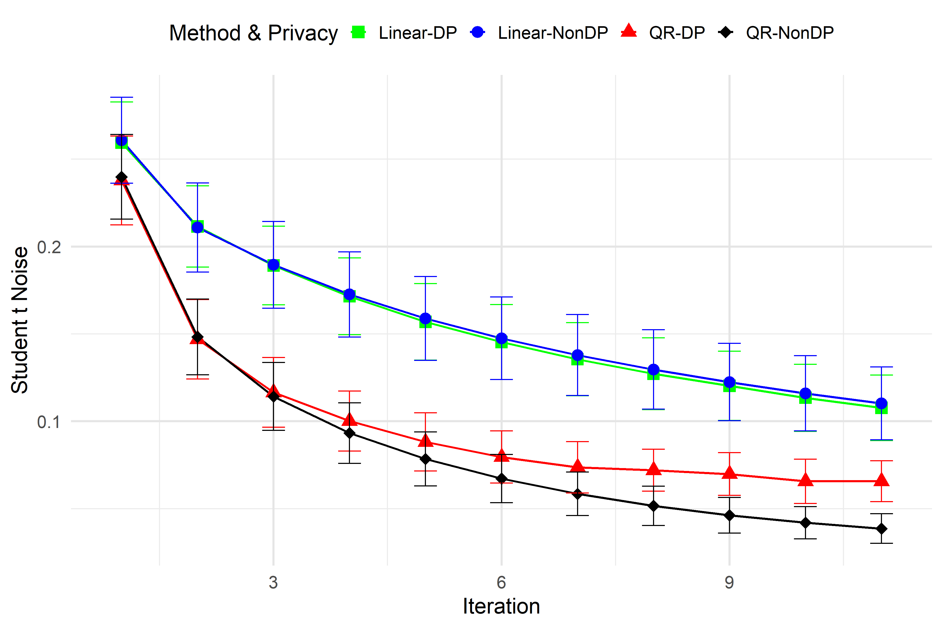
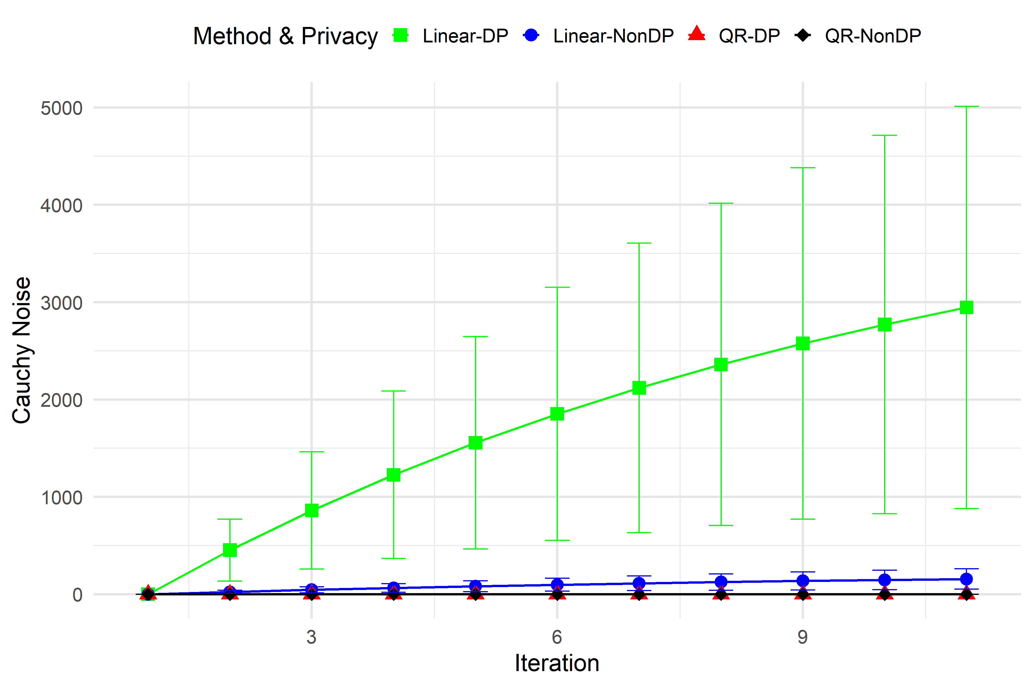
The case of heteroscedastic errors

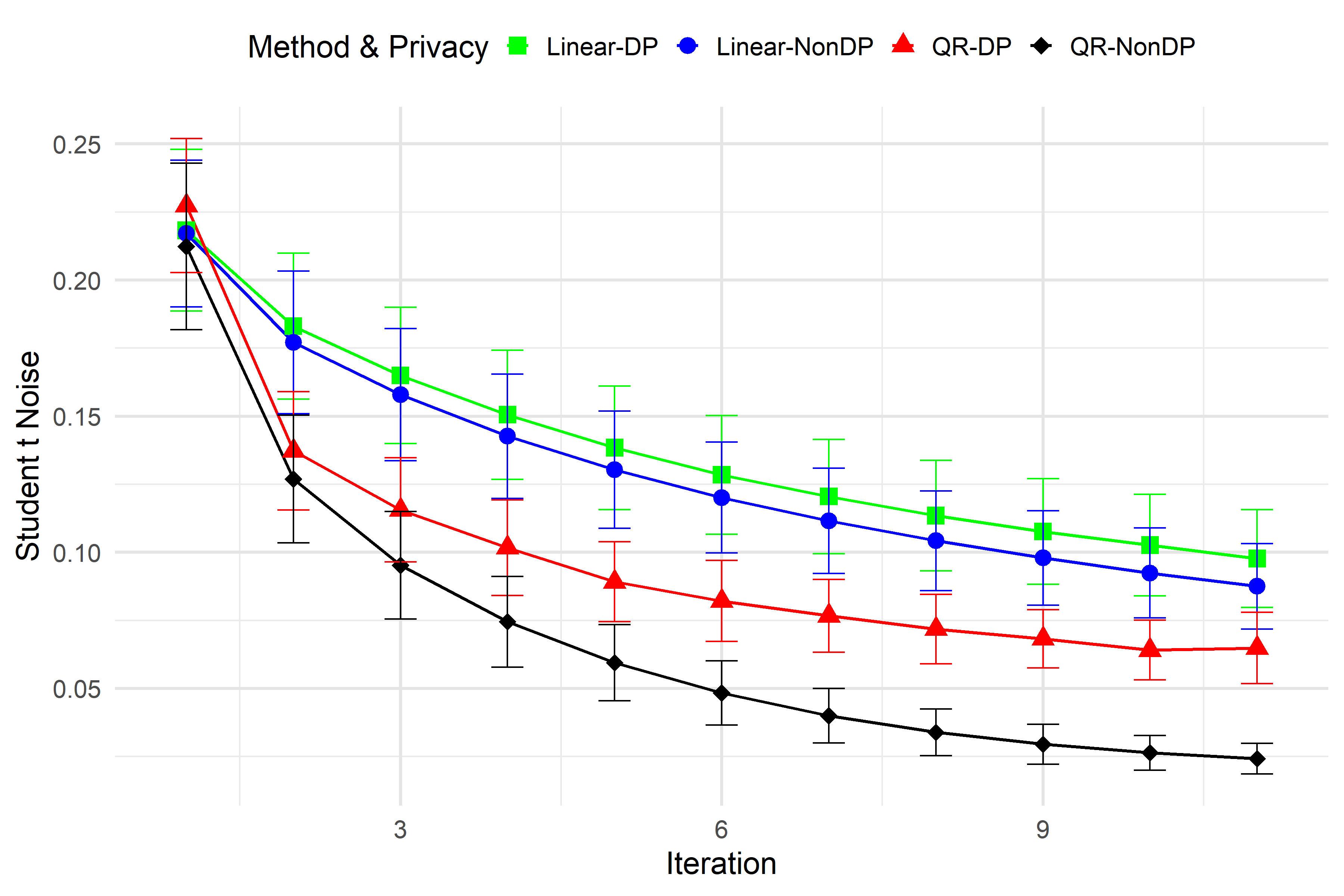
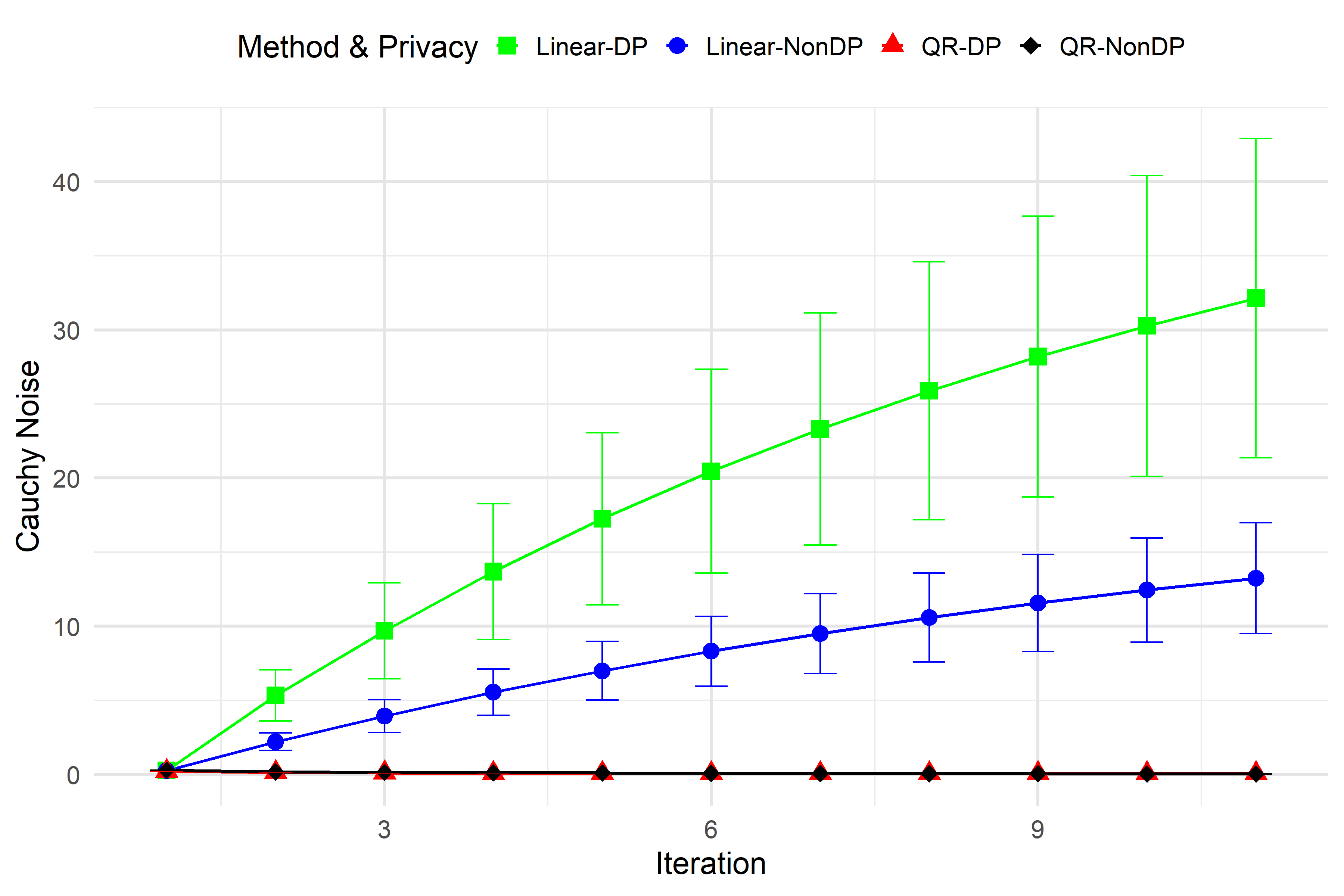
Figure 1 compares our quantile regression (QR) method ($T=10,K=10$) with the distributed linear regression approach of [8]. Each iteration $t$ consists of 10 gradient descent steps. Results are shown for three noise types. In all scenarios, the QR estimator achieves lower $\ell_{2}$-error than the linear regression baseline, regardless of whether differential privacy (DP) is enforced. Under Cauchy noise, the linear regression estimators fail to converge due to the infinite moments of the Cauchy distribution. Both DP and non-DP versions exhibit diverging errors, highlighting their unreliability in heavy-tailed settings. In contrast, the QR estimators remain stable and continue to converge. A consistent pattern emerges regarding privacy: DP versions of all methods exhibit larger long-term errors than their non-private counterparts. This observation aligns with the theoretical results in Section 3, where the additional error from DP is characterized as the inherent cost of privacy protection.

Figure 2: $\ell_{2}$ error v.s. iteration $t$ for different noise distributions, differentially private parameters, and variance types. (Fix $N=20000,n=500$.)

The case of homoscedastic errors

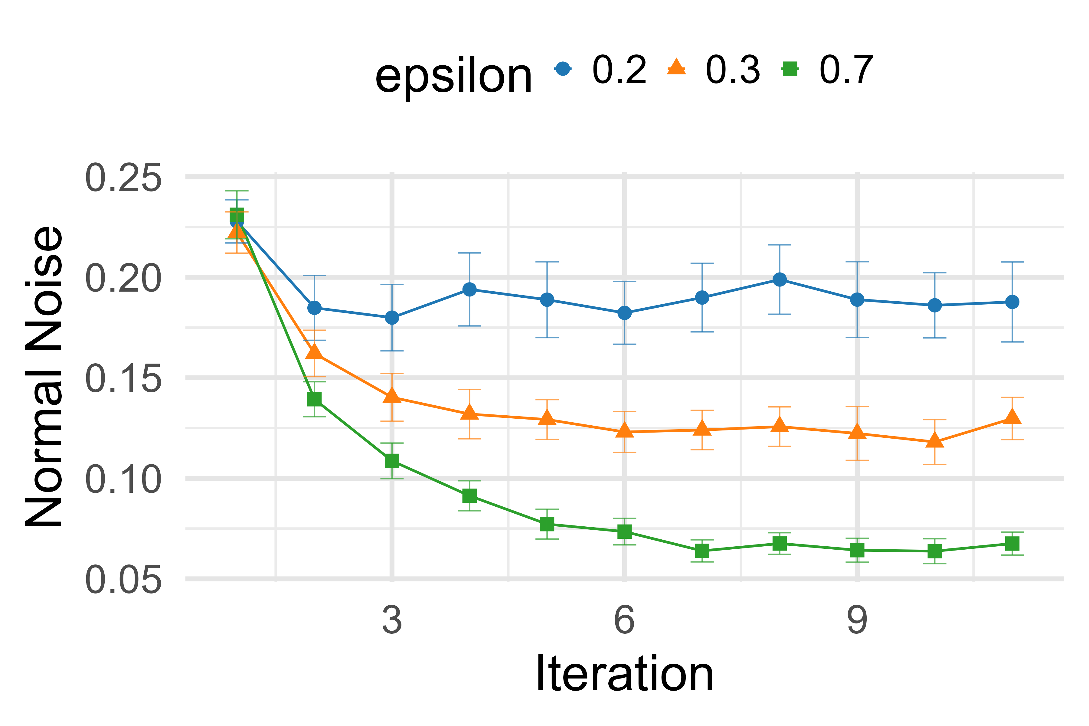
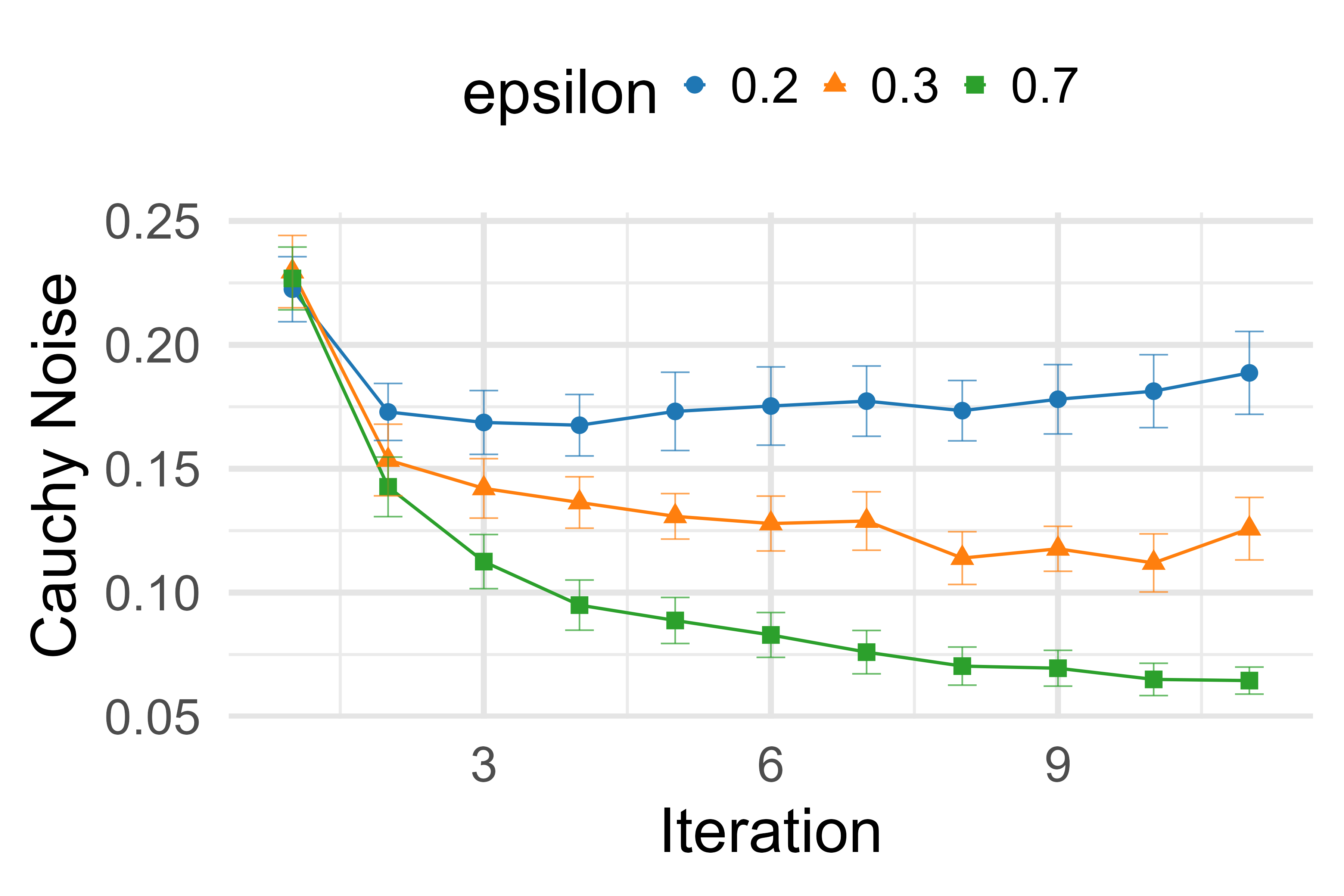
The case of heteroscedastic errors

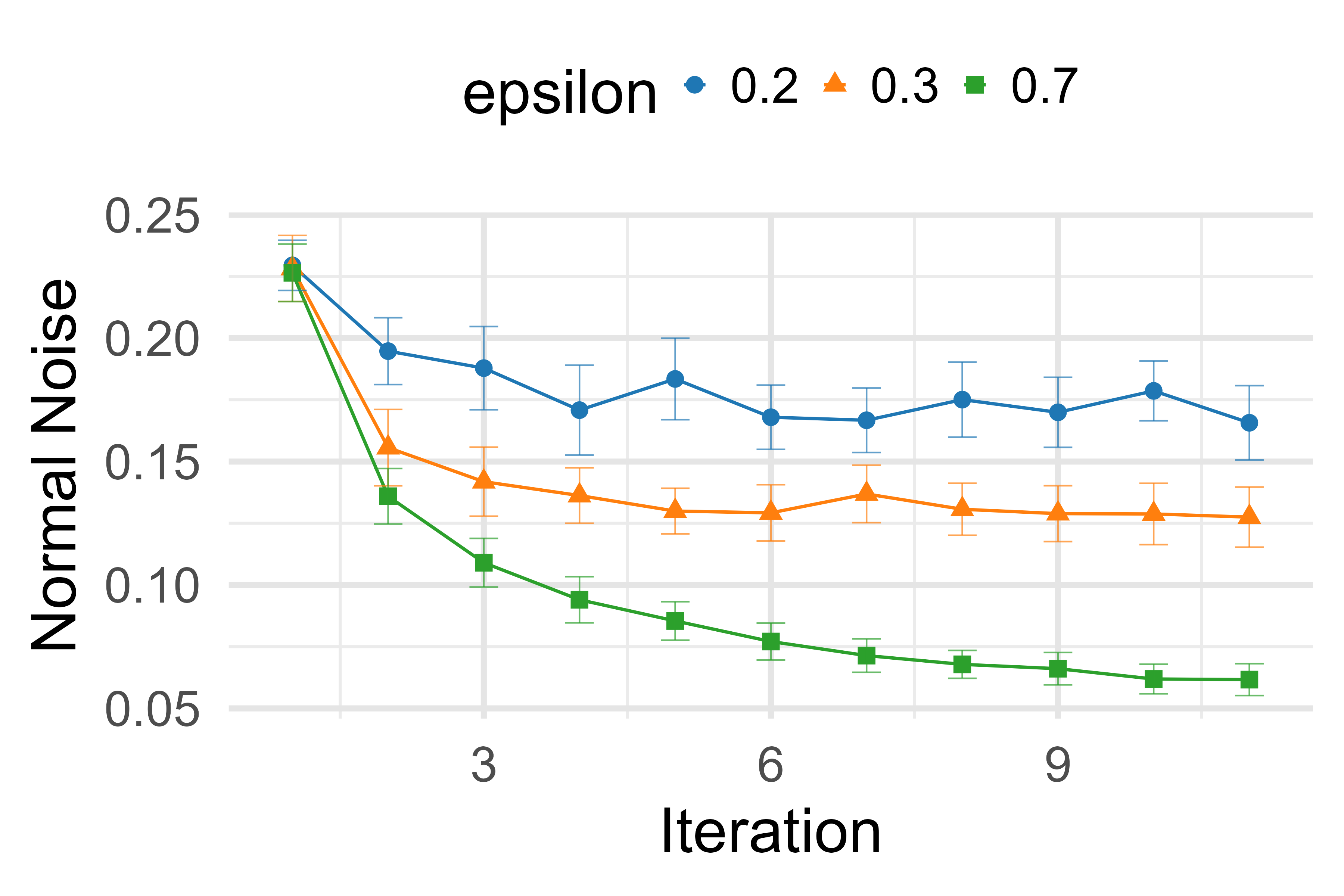
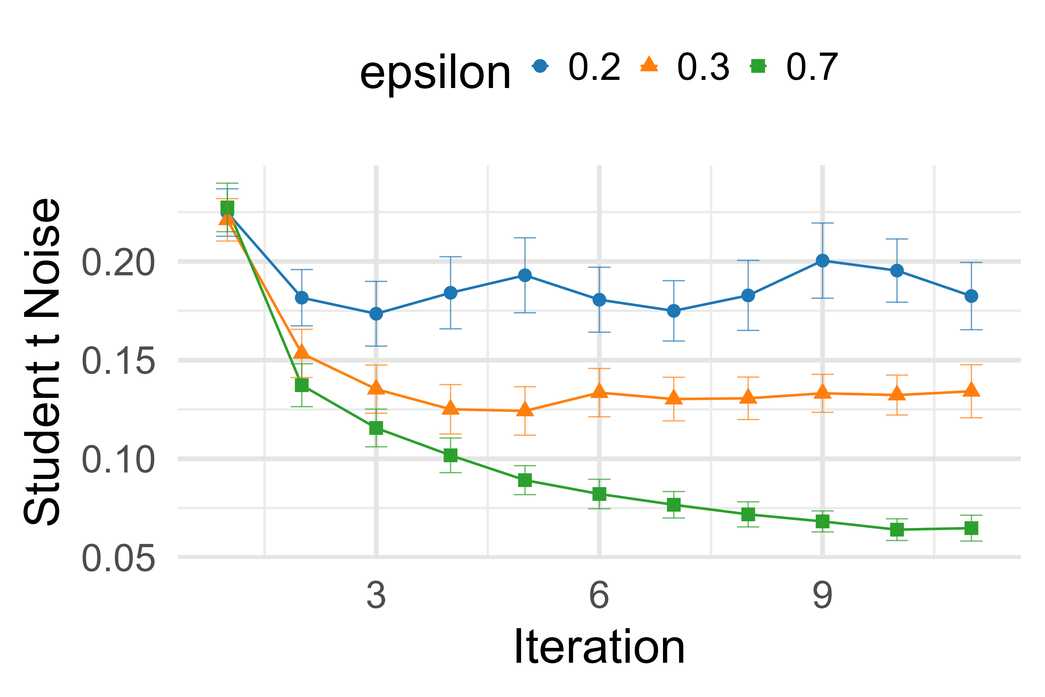
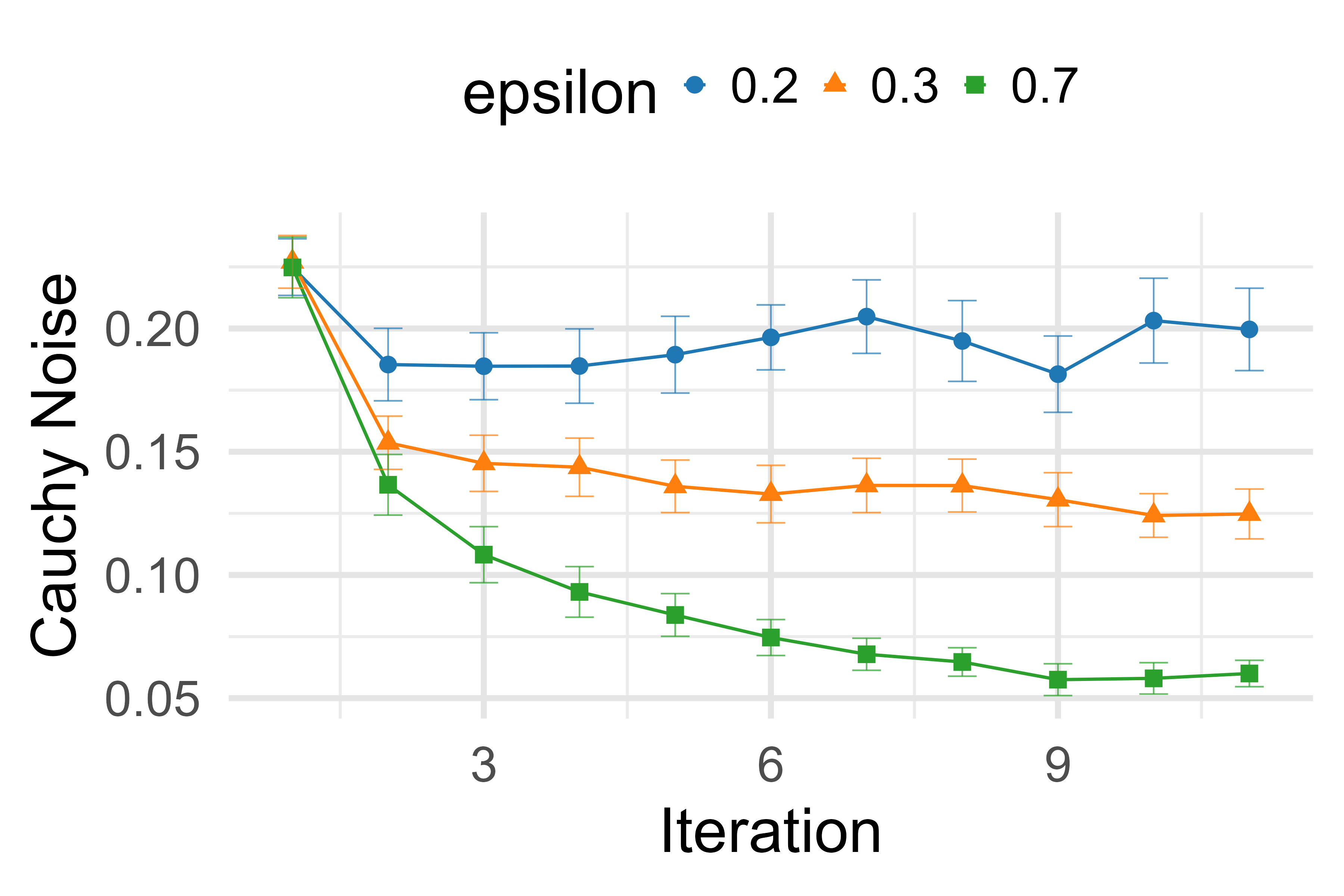
To better understand how varying levels of privacy protection influence the convergence rate in high-dimensional differentially private quantile regression, we examine the estimator’s behavior as the privacy budget $\epsilon$ changes. As shown in Figure 2, smaller values of $\epsilon$ (corresponding to stronger privacy guarantees) consistently lead to larger long-term estimation errors. This monotonic increase in error with stricter privacy aligns closely with the theoretical prediction in Theorem 2, where the error term $\mathcal{O}\left(\sqrt{\frac{(s^{*}\log p)^{2}\log(1/\delta)\log^{3}N}{N^{2}\epsilon^{2}}}\right)$ quantifies the fundamental trade-off between privacy protection and statistical accuracy.

Table 1: The $\ell_{2}$-error varying different privacy, noise type, and total sample size $N$ under homoscedastic error case. (Fix the local sample size $n=500$.)

Noise	Normal			$t(3)$			Cauchy
$N$	5000	10000	20000	5000	10000	20000	5000	10000	20000
$\epsilon=0.1$	0.389(0.183)	0.344(0.120)	0.419(0.208)	0.407(0.201)	0.421(0.221)	0.447(0.258)	0.451(0.243)	0.434(0.208)	0.520(0.282)
$\epsilon=0.2$	0.193(0.063)	0.172(0.059)	0.191(0.071)	0.194(0.057)	0.186(0.056)	0.187(0.075)	0.210(0.059)	0.206(0.079)	0.208(0.069)
$\epsilon=0.5$	0.086(0.031)	0.086(0.033)	0.074(0.023)	0.091(0.032)	0.085(0.024)	0.083(0.038)	0.107(0.037)	0.102(0.037)	0.102(0.035)
$\epsilon=0.7$	0.071(0.027)	0.064(0.022)	0.065(0.026)	0.083(0.029)	0.070(0.023)	0.070(0.023)	0.089(0.035)	0.081(0.025)	0.077(0.026)
$\epsilon=1$	0.069(0.002)	0.053(0.017)	0.049(0.016)	0.071(0.025)	0.061(0.025)	0.053(0.020)	0.079(0.031)	0.073(0.027)	0.066(0.027)

Table 2: The $\ell_{2}$-error varying different privacy, noise type, and total sample size $N$ under heteroscedastic error case. (Fix the local sample size $n=500$.)

Noise	Normal			$t(3)$			Cauchy
$N$	5000	10000	20000	5000	10000	20000	5000	10000	20000
$\epsilon=0.1$	0.333(0.127)	0.361(0.171)	0.341(0.167)	0.407(0.268)	0.407(0.268)	0.447(0.259)	0.441(0.283)	0.431(0.290)	0.468(0.260)
$\epsilon=0.2$	0.166(0.065)	0.107(0.062)	0.177(0.071)	0.170(0.060)	0.164(0.062)	0.160(0.058)	0.160(0.055)	0.168(0.065)	0.184(0.069)
$\epsilon=0.5$	0.078(0.027)	0.072(0.025)	0.073(0.024)	0.079(0.030)	0.072(0.028)	0.072(0.021)	0.091(0.038)	0.085(0.031)	0.075(0.024)
$\epsilon=0.7$	0.059(0.020)	0.052(0.016)	0.050(0.021)	0.063(0.021)	0.057(0.021)	0.056(0.018)	0.074(0.029)	0.063(0.024)	0.066(0.024)
$\epsilon=1$	0.049(0.017)	0.044(0.015)	0.043(0.016)	0.059(0.018)	0.045(0.018)	0.043(0.013)	0.065(0.027)	0.057(0.018)	0.057(0.025)

Table 3: The $\ell_{2}$-error varying different privacy, noise type, and local sample size $n$ under homoscedastic error case. (Fix the total sample size $N=20000$.)

Noise	Normal			$t(3)$			Cauchy
$n$	500	1000	2000	500	1000	2000	500	1000	2000
$\epsilon=0.1$	0.475(0.326)	0.193(0.084)	0.094(0.031)	0.537(0.293)	0.178(0.068)	0.105(0.030)	0.445(0.210)	0.219(0.073)	0.096(0.034)
$\epsilon=0.2$	0.192(0.053)	0.085(0.031)	0.047(0.014)	0.187(0.061)	0.113(0.037)	0.046(0.014)	0.195(0.065)	0.107(0.045)	0.061(0.020)
$\epsilon=0.5$	0.072(0.023)	0.045(0.019)	0.030(0.011)	0.081(0.042)	0.051(0.018)	0.033(0.015)	0.093(0.028)	0.055(0.015)	0.044(0.017)
$\epsilon=0.7$	0.054(0.017)	0.042(0.015)	0.028(0.012)	0.065(0.022)	0.046(0.016)	0.030(0.010)	0.088(0.028)	0.049(0.016)	0.037(0.012)
$\epsilon=1$	0.048(0.019)	0.039(0.014)	0.026(0.007)	0.050(0.022)	0.040(0.014)	0.030(0.009)	0.076(0.028)	0.048(0.016)	0.035(0.011)

Table 4: The $\ell_{2}$-error varying different privacy, noise type, and local sample size $n$ under heteroscedastic error case. (Fix the total sample size $N=20000$.)

Noise	Normal			$t(3)$			Cauchy
$n$	500	1000	2000	500	1000	2000	500	1000	2000
$\epsilon=0.1$	0.372(0.192)	0.177(0.069)	0.075(0.028)	0.388(0.188)	0.164(0.047)	0.087(0.039)	0.471(0.233)	0.187(0.064)	0.101(0.046)
$\epsilon=0.2$	0.166(0.055)	0.077(0.031)	0.040(0.011)	0.165(0.057)	0.082(0.035)	0.048(0.016)	0.198(0.058)	0.102(0.070)	0.054(0.019)
$\epsilon=0.5$	0.057(0.015)	0.036(0.013)	0.026(0.010)	0.083(0.030)	0.036(0.012)	0.029(0.008)	0.079(0.028)	0.044(0.020)	0.031(0.009)
$\epsilon=0.7$	0.055(0.017)	0.032(0.012)	0.022(0.010)	0.050(0.020)	0.034(0.068)	0.026(0.010)	0.060(0.012)	0.038(0.014)	0.030(0.010)
$\epsilon=1$	0.040(0.011)	0.024(0.006)	0.020(0.005)	0.043(0.016)	0.028(0.008)	0.023(0.008)	0.055(0.016)	0.034(0.011)	0.026(0.008)

Tables 1–4 comprehensively quantify the privacy-accuracy-efficiency trade-offs under fixed computational budgets ($K=T=10$) and varying privacy budgets $\epsilon$. Three principal empirical patterns emerge from these analyses.

First, across all noise distributions and data models—including both homoscedastic (Model 1) and heteroscedastic (Model 2) error structures—strengthening privacy protection systematically increases the $\ell_{2}$-error, with mean error rising as $\epsilon$ decreases from 1.0 to 0.1. This monotonic relationship provides empirical validation for the DP error term in our theoretical framework.

Second, as shown in Tables 1-2, the interaction between privacy constraints and sample efficiency reveals a fundamental dichotomy. Under relaxed privacy regimes (e.g., $\epsilon\geq 0.5$), the $\ell_{2}$-error decreases as the total sample size $N$ increases, indicating that the oracle convergence rate dominates when privacy costs are moderate. Conversely, under strict privacy (e.g., $\epsilon<0.5$), error reduction plateaus despite increasing $N$, demonstrating that privacy-induced error becomes the limiting factor in highly constrained settings. This pattern persists even in the presence of heteroscedasticity.

Third, as shown in Tables 3-4, increasing the local sample size $n$ while fixing the global sample size $N=20000$ consistently reduces the $\ell_{2}$-error across all privacy levels. Since we use $K=T=10$ and take the single-machine estimate as the starting point, this trend reflects the influence of the initial estimator, as captured by the third term in (15).

6.2 Inference Simulation

In this section, we conduct simulation studies to evaluate the inference performance of our proposed differentially private distributed quantile regression methods. Specifically, we focus on two key aspects: (1) assessing the normality of the standardized test statistics, and (2) evaluating the empirical coverage and width of simultaneous confidence intervals constructed via two bootstrap-based procedures. The data generation process and privacy parameter settings are the same as in the estimation experiments. We fix the number of outer iterations at $T=10$, set the local bandwidth to $b=0.5\cdot(\log p/n)^{1/3}$, and use the median quantile level $\tau=0.5$. The total sample size is $N=20{,}000$, with local sample size $n=500$. For the bootstrap procedures, we use $n_{B}=2000$ replications and set the significance level to $\alpha=5\%$.

Figure 3: Histograms and QQ plots of the standardized test statistics at $\tau=0.5$, under Normal, $t(3)$, and Cauchy noises ($\epsilon=1$, $n=500$ and $N=5000$). Rows represent noise types, columns correspond to $\beta_{j}$.

The case of homoscedastic errors: Histograms

Figure 4: Histograms and QQ plots of the standardized test statistics at $\tau=0.5$, under Normal, $t(3)$, and Cauchy noises ($\epsilon=1$, $n=500$ and $N=5000$). Rows represent noise types, columns correspond to $\beta_{j}$.

The case of heteroscedastic errors: Histograms

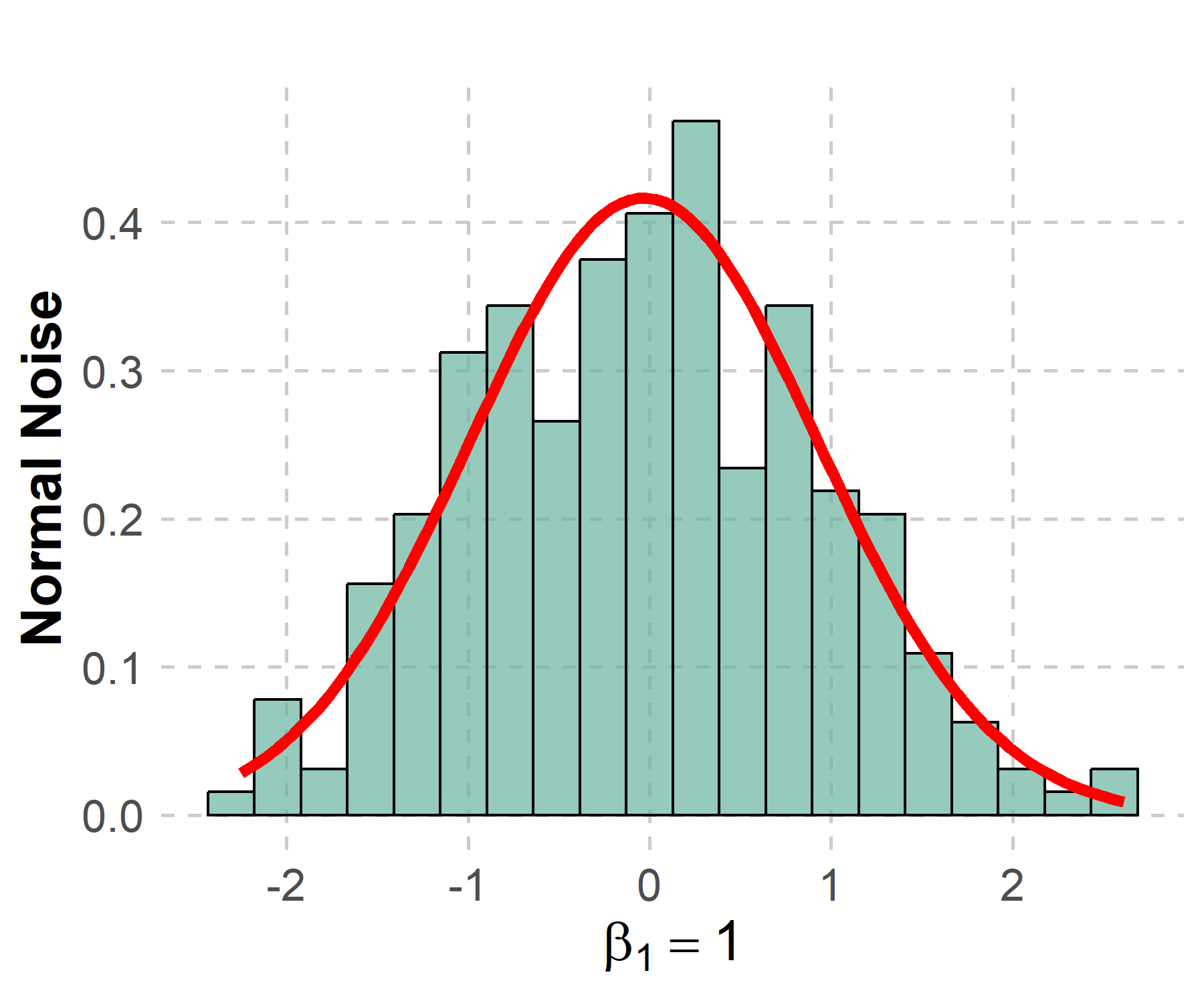
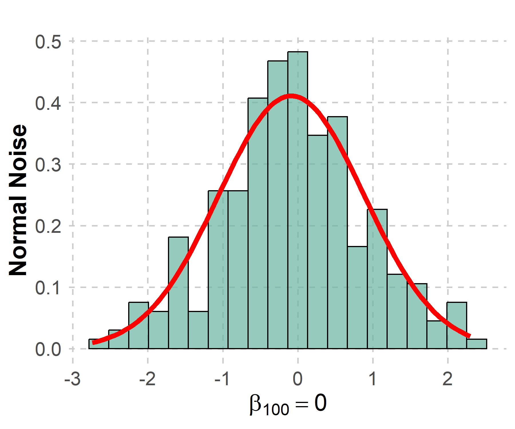
Figures 3 and 4 display the distributions of the standardized test statistic

$$z_{j}=\frac{\sqrt{mn}(\widetilde{\beta}_{j}-\beta^{*}_{j})}{\sqrt{\frac{1}{m}\sum_{k=1}^{m}\widehat{\sigma}^{(k)}+\frac{8B_{2}^{2}\log(1/\delta)}{mn\epsilon^{2}}}}$$

for $j=1$ and $j=100$ under different null hypothesis settings. Across all noise types, the histograms demonstrate that $z_{j}$ closely follows the standard normal distribution, even in the presence of heavy-tailed errors. This indicates that our inference procedure remains robust for both strong and weak signals. The accompanying Q-Q plots compare the empirical quantiles of $z_{j}$ with those of the standard normal distribution. The close alignment of points along the $\mathrm{y}=\mathrm{x}$ line further confirms the approximate normality of $z_{j}$. These empirical findings are consistent with the theoretical results established in Section 4.

Figure 5: Simultaneous Confidence intervals for $\beta_{k}$ for each coordinate $k$. (The case of heteroscedastic errors with Cauchy noise, $m=10$, $\epsilon=1,\delta=1/N$).

Figure 5 demonstrates the effectiveness of our distributed bootstrap simultaneous inference procedure (Algorithm 5) by presenting 95% simultaneous confidence intervals for all model parameters. For visualization, we display the complete set of parameter estimates for non-sparse subsets and a representative subset of 45 randomly selected parameters for sparse subsets. The constructed intervals consistently achieve full coverage of the true parameter values (indicated by dashed reference lines), while maintaining practical interval widths. Importantly, our bootstrap framework automatically accounts for parameter dependencies, eliminating the need for explicit covariance matrix estimation. The uniformity of interval widths across parameters of varying magnitudes further highlights the robustness of our error control mechanism. Figure 5 also specifically illustrates the scenario with a small number of machines ($m=10$). In this setting, the $\mathsf{(n+k-1)\text{-}grad}$ method yields consistently narrower confidence intervals compared to the $\mathsf{k\text{-}grad}$ approach at the same significance level, demonstrating its superior efficiency for smaller $m$. These experimental findings are fully consistent with the theoretical comparisons of the two bootstrap strategies presented in Section 5.

6.3 Sensitivity Analysis for the Sparsity

This section investigates the sensitivity of distributed quantile regression estimators to the choice of the sparsity parameter $s$. Theoretical results guarantee exact support recovery for DHSQR under heteroscedastic errors [15] and DREL under homoscedastic errors [14], provided sub-Gaussian noise and standard regularity conditions hold (see Theorem 3.10 in [15] and Theorem 5 in [14]). Notably, these approaches do not require prior knowledge of the true sparsity level $s^{*}$; it suffices to specify any $s\geq s^{*}$ for consistent estimation.

To empirically assess the impact of sparsity specification, we report the $\ell_{2}$-error for a range of sparsity levels $s\in\{5,6,\dots,10,20,30,40,50\}$ under heteroscedastic errors with true sparsity $s^{*}=5$. As shown in Table 5, the estimation error remains stable for $s$ up to approximately $2s^{*}$, indicating that moderate overspecification does not degrade performance. However, when $s$ exceeds $4s^{*}$, the $\ell_{2}$-error increases monotonically, reflecting the loss of efficiency due to excessive regularization.

Table 5: The $\ell_{2}$-error varying sparsity under heteroscedastic error case. (Fix the total sample size $N=20000$.)

Noise	Normal			$t(3)$			Cauchy
Sparsity	$\epsilon=0.5$	$\epsilon=0.7$	$\epsilon=1$	$\epsilon=0.5$	$\epsilon=0.7$	$\epsilon=1$	$\epsilon=0.5$	$\epsilon=0.7$	$\epsilon=1$
5	0.064(0.017)	0.050(0.016)	0.040(0.015)	0.071(0.027)	0.058(0.023)	0.047(0.017)	0.070(0.027)	0.064(0.022)	0.080(0.025)
6	0.077(0.027)	0.060(0.019)	0.043(0.016)	0.078(0.034)	0.060(0.017)	0.045(0.031)	0.082(0.045)	0.069(0.027)	0.049(0.025)
7	0.084(0.026)	0.069(0.021)	0.047(0.013)	0.082(0.021)	0.066(0.019)	0.044(0.013)	0.090(0.024)	0.073(0.032)	0.049(0.018)
8	0.097(0.030)	0.079(0.028)	0.047(0.017)	0.095(0.034)	0.079(0.026)	0.041(0.019)	0.091(0.032)	0.073(0.031)	0.041(0.018)
9	0.097(0.030)	0.083(0.026)	0.052(0.017)	0.095(0.031)	0.087(0.025)	0.050(0.014)	0.097(0.029)	0.087(0.025)	0.055(0.018)
10	0.117(0.039)	0.080(0.024)	0.058(0.016)	0.116(0.041)	0.087(0.025)	0.061(0.020)	0.122(0.034)	0.088(0.025)	0.057(0.019)
20	0.202(0.048)	0.144(0.026)	0.101(0.025)	0.201(0.070)	0.146(0.033)	0.102(0.024)	0.204(0.054)	0.154(0.029)	0.101(0.021)
30	0.301(0.049)	0.216(0.051)	0.148(0.027)	0.314(0.057)	0.221(0.048)	0.151(0.026)	0.321(0.054)	0.232(0.039)	0.155(0.031)
40	0.406(0.055)	0.276(0.036)	0.198(0.035)	0.414(0.063)	0.274(0.048)	0.201(0.045)	0.422(0.051)	0.231(0.048)	0.202(0.049)
50	0.485(0.065)	0.357(0.055)	0.243(0.035)	0.487(0.062)	0.366(0.064)	0.251(0.038)	0.489(0.065)	0.368(0.057)	0.247(0.032)

7 Conclusion and Future Work

In this work, we studied distributed high-dimensional quantile regression under differential privacy, providing both theoretical guarantees and practical algorithms. Our results show that the final estimation error decomposes into two main components: the oracle convergence rate and the additional error due to privacy, consistent with the “cost of privacy” established in [7]. For inference, we demonstrated that the debiased estimator achieves asymptotic normality, enabling valid confidence intervals and hypothesis testing. Furthermore, we developed a differentially private multiplier bootstrap procedure for simultaneous inference in high dimensions. Extensive simulations confirm that our methods achieve robust estimation and inference with moderate privacy budgets, while excessive privacy protection can impede statistical accuracy, highlighting the fundamental privacy-accuracy trade-off.

Future research directions include extending our framework to more complex models, such as expectile regression, expected shortfall regression, support vector machines, and functional regression, thereby broadening the applicability of privacy-preserving statistical learning. Another important avenue is the development of advanced privacy mechanisms—such as local differential privacy and Gaussian differential privacy—for high-dimensional settings, to further improve the balance between privacy and statistical efficiency [9, 27, 30]. Finally, we note that sparsity-aware privacy methods can go beyond simple thresholding; for example, algorithms like DP-ADMM [65] offer more flexible trade-offs between privacy and performance. Adapting such optimization techniques to high-dimensional problems remains a promising direction for future work.

References

- [1] C. Dwork, F. McSherry, K. Nissim, and A. Smith, “Calibrating noise to sensitivity in private data analysis,” in Theory of Cryptography: Third Theory of Cryptography Conference, TCC 2006, New York, NY, USA, March 4-7, 2006. Proceedings 3, pp. 265–284, Springer, 2006.
- [2] C. Dwork, K. Kenthapadi, F. McSherry, I. Mironov, and M. Naor, “Our data, ourselves: Privacy via distributed noise generation,” in Advances in Cryptology-EUROCRYPT 2006: 24th Annual International Conference on the Theory and Applications of Cryptographic Techniques, St. Petersburg, Russia, May 28-June 1, 2006. Proceedings 25, pp. 486–503, Springer, 2006.
- [3] C. Dwork, A. Roth, et al., “The algorithmic foundations of differential privacy,” Foundations and Trends® in Theoretical Computer Science, vol. 9, no. 3–4, pp. 211–407, 2014.
- [4] G. Barthe and B. Kopf, “Information-theoretic bounds for differentially private mechanisms,” in 2011 IEEE 24th Computer Security Foundations Symposium, pp. 191–204, IEEE, 2011.
- [5] R. Koenker and G. Bassett Jr, “Regression quantiles,” Econometrica, vol. 46, no. 1, pp. 33–50, 1978.
- [6] R. Koenker, Quantile Regression, vol. 38. Cambridge University Press, 2005.
- [7] T. T. Cai, Y. Wang, and L. Zhang, “The cost of privacy: Optimal rates of convergence for parameter estimation with differential privacy,” The Annals of Statistics, vol. 49, no. 5, pp. 2825–2850, 2021.
- [8] Z. Zhang, R. Nakada, and L. Zhang, “Differentially private federated learning: Servers trustworthiness, estimation, and statistical inference,” arXiv preprint arXiv:2404.16287, 2024.
- [9] D. Wang and J. Xu, “On sparse linear regression in the local differential privacy model,” IEEE Transactions on Information Theory, vol. 67, no. 2, pp. 1182–1200, 2020.
- [10] N. Agarwal, A. T. Suresh, F. Yu, S. Kumar, and H. B. McMahan, “cpsgd: communication-efficient and differentially-private distributed sgd,” in Proceedings of the 32nd International Conference on Neural Information Processing Systems, p. 7575–7586, Curran Associates Inc., 2018.
- [11] Ú. Erlingsson, V. Feldman, I. Mironov, A. Raghunathan, S. Song, K. Talwar, and A. Thakurta, “Encode, shuffle, analyze privacy revisited: Formalizations and empirical evaluation,” arXiv preprint arXiv:2001.03618, 2020.
- [12] A. Bittau, Ú. Erlingsson, P. Maniatis, I. Mironov, A. Raghunathan, D. Lie, M. Rudominer, U. Kode, J. Tinnes, and B. Seefeld, “Prochlo: Strong privacy for analytics in the crowd,” in Proceedings of the 26th Symposium on Operating Systems Principles, pp. 441–459, 2017.
- [13] A. Girgis, D. Data, S. Diggavi, P. Kairouz, and A. Theertha Suresh, “Shuffled model of differential privacy in federated learning,” in Proceedings of The 24th International Conference on Artificial Intelligence and Statistics (A. Banerjee and K. Fukumizu, eds.), vol. 130 of Proceedings of Machine Learning Research, pp. 2521–2529, PMLR, 13–15 Apr 2021.
- [14] X. Chen, W. Liu, X. Mao, and Z. Yang, “Distributed high-dimensional regression under a quantile loss function,” Journal of Machine Learning Research, vol. 21, no. 182, pp. 1–43, 2020.
- [15] C. Wang and Z. Shen, “Distributed high-dimensional quantile regression: Estimation efficiency and support recovery,” in Proceedings of the 41st International Conference on Machine Learning, pp. 51415–51441, 2024.
- [16] J. C. Duchi, M. I. Jordan, and M. J. Wainwright, “Local privacy and statistical minimax rates,” in 2013 IEEE 54th Annual Symposium on Foundations of Computer Science, pp. 429–438, IEEE, 2013.
- [17] J. Dong, A. Roth, and W. J. Su, “Gaussian differential privacy,” Journal of the Royal Statistical Society Series B: Statistical Methodology, vol. 84, no. 1, pp. 3–37, 2022.
- [18] I. Dinur and K. Nissim, “Revealing information while preserving privacy,” in Proceedings of the 22nd ACM SIGMOD-SIGACT-SIGART Symposium on Principles of Database Systems, pp. 202–210, 2003.
- [19] C. Dwork, F. McSherry, and K. Talwar, “The price of privacy and the limits of LP decoding,” in Proceedings of the 39th Annual ACM Symposium on Theory of Computing, pp. 85–94, 2007.
- [20] C. Dwork and S. Yekhanin, “New efficient attacks on statistical disclosure control mechanisms,” in Proceedings of the 28th Annual Conference on Cryptology: Advances in Cryptology, p. 469–480, Springer, Springer-Verlag, 2008.
- [21] M. Yu, Z. Ren, and W.-X. Zhou, “Gaussian differentially private robust mean estimation and inference,” Bernoulli, vol. 30, no. 4, pp. 3059–3088, 2024.
- [22] X. Liu, W. Kong, S. Kakade, and S. Oh, “Robust and differentially private mean estimation,” in Proceedings of the 35th International Conference on Neural Information Processing Systems, pp. 3887–3901, 2021.
- [23] S. Agarwal, G. Kamath, M. Majid, A. Mouzakis, R. Silver, and J. Ullman, “Private mean estimation with person-level differential privacy,” in Proceedings of the 2025 Annual ACM-SIAM Symposium on Discrete Algorithms, pp. 2819–2880, SIAM, 2025.
- [24] K. Amin, T. Dick, A. Kulesza, A. M. Medina, and S. Vassilvitskii, “Differentially private covariance estimation,” in Proceedings of the 33rd International Conference on Neural Information Processing Systems, pp. 14213–14222, 2019.
- [25] D. G. Alabi and S. P. Vadhan, “Differentially private hypothesis testing for linear regression,” Journal of Machine Learning Research, vol. 24, no. 361, pp. 1–50, 2023.
- [26] O. Sheffet, “Differentially private ordinary least squares,” in Proceedings of the 34th International Conference on Machine Learning-Volume 70, pp. 3105–3114, 2017.
- [27] H. Asi, V. Feldman, and K. Talwar, “Optimal algorithms for mean estimation under local differential privacy,” in Proceedings of the 39th International Conference on Machine Learning, vol. 162 of Proceedings of Machine Learning Research, pp. 1046–1056, PMLR, 17–23 Jul 2022.
- [28] J. C. Duchi, M. I. Jordan, and M. J. Wainwright, “Minimax optimal procedures for locally private estimation,” Journal of the American Statistical Association, vol. 113, no. 521, pp. 182–201, 2018.
- [29] M. Avella-Medina, C. Bradshaw, and P.-L. Loh, “Differentially private inference via noisy optimization,” The Annals of Statistics, vol. 51, no. 5, pp. 2067–2092, 2023.
- [30] M. Li, T. B. Berrett, and Y. Yu, “On robustness and local differential privacy,” The Annals of Statistics, vol. 51, no. 2, pp. 717–737, 2023.
- [31] G. Kamath, A. Mouzakis, M. Regehr, V. Singhal, T. Steinke, and J. Ullman, “A bias-accuracy-privacy trilemma for statistical estimation,” Journal of the American Statistical Association, 2025. in press.
- [32] C. Dwork, W. Su, and L. Zhang, “Differentially private false discovery rate control,” Journal of Privacy and Confidentiality, vol. 11, Sep. 2021.
- [33] X. Xia and Z. Cai, “Adaptive false discovery rate control with privacy guarantee,” Journal of Machine Learning Research, vol. 24, no. 252, pp. 1–35, 2023.
- [34] Z. Cai, S. Li, X. Xia, and L. Zhang, “Private estimation and inference in high-dimensional regression with FDR control,” arXiv preprint arXiv:2310.16260, 2023.
- [35] T. Steinke and J. Ullman, “Tight lower bounds for differentially private selection,” in 2017 IEEE 58th Annual Symposium on Foundations of Computer Science, pp. 552–563, IEEE, 2017.
- [36] W. Dong, Y. Liang, and K. Yi, “Differentially private covariance revisited,” in Proceedings of the 36th International Conference on Neural Information Processing Systems, pp. 850–861, 2022.
- [37] K. Talwar, A. Thakurta, and L. Zhang, “Nearly-optimal private lasso,” in Proceedings of the 29th International Conference on Neural Information Processing Systems-Volume 2, pp. 3025–3033, 2015.
- [38] W. Liu, X. Mao, X. Zhang, and X. Zhang, “Efficient sparse least absolute deviation regression with differential privacy,” IEEE Transactions on Information Forensics and Security, vol. 19, pp. 2328–2339, 2024.
- [39] C. Dwork, P. Tankala, and L. Zhang, “Differentially private learning beyond the classical dimensionality regime,” arXiv preprint arXiv:2411.13682, 2024.
- [40] T. Blumensath and M. E. Davies, “Iterative hard thresholding for compressed sensing,” Applied and Computational Harmonic Analysis, vol. 27, no. 3, pp. 265–274, 2009.
- [41] T. T. Cai, Y. Wang, and L. Zhang, “Score attack: A lower bound technique for optimal differentially private learning,” arXiv preprint arXiv:2303.07152, 2023.
- [42] E. Bao, D. Gao, X. Xiao, and Y. Li, “Communication efficient and differentially private logistic regression under the distributed setting,” in Proceedings of the 29th ACM SIGKDD Conference on Knowledge Discovery and Data Mining, pp. 69–79, 2023.
- [43] C. Gao, A. Lowy, X. Zhou, and S. J. Wright, “Private heterogeneous federated learning without a trusted server revisited: Error-optimal and communication-efficient algorithms for convex losses,” arXiv preprint arXiv:2407.09690, 2024.
- [44] H. Wang and C. Li, “Distributed quantile regression over sensor networks,” IEEE Transactions on Signal and Information Processing over Networks, vol. 4, no. 2, pp. 338–348, 2017.
- [45] T. T. Cai, A. Chakraborty, and L. Vuursteen, “Optimal federated learning for nonparametric regression with heterogeneous distributed differential privacy constraints,” arXiv preprint arXiv:2406.06755, 2024.
- [46] T. T. Cai, A. Chakraborty, and L. Vuursteen, “Federated nonparametric hypothesis testing with differential privacy constraints: Optimal rates and adaptive tests,” arXiv preprint arXiv:2406.06749, 2024.
- [47] L. Vuursteen, “Optimal private and communication constraint distributed goodness-of-fit testing for discrete distributions in the large sample regime,” arXiv preprint arXiv:2411.01275, 2024.
- [48] A. Auddy, T. T. Cai, and A. Chakraborty, “Minimax and adaptive transfer learning for nonparametric classification under distributed differential privacy constraints,” arXiv preprint arXiv:2406.20088, 2024.
- [49] M. Li, Y. Tian, Y. Feng, and Y. Yu, “Federated transfer learning with differential privacy,” arXiv preprint arXiv:2403.11343, 2024.
- [50] X. He, X. Pan, K. M. Tan, and W.-X. Zhou, “Smoothed quantile regression with large-scale inference,” Journal of Econometrics, vol. 232, no. 2, pp. 367–388, 2023.
- [51] M. Schmidt, “Graphical model structure learning with l1-regularization,” University of British Columbia, 2010.
- [52] S. J. Wright, “Coordinate descent algorithms,” Mathematical Programming, vol. 151, no. 1, pp. 3–34, 2015.
- [53] X. Chen, W. Liu, and Y. Zhang, “Quantile regression under memory constraint,” The Annals of Statistics, vol. 47, no. 6, pp. 3244–3273, 2019.
- [54] Y. Yan, X. Wang, and R. Zhang, “Confidence intervals and hypothesis testing for high-dimensional quantile regression: Convolution smoothing and debiasing,” Journal of Machine Learning Research, vol. 24, no. 245, pp. 1–49, 2023.
- [55] D. Wang and J. Xu, “Differentially private high dimensional sparse covariance matrix estimation,” Theoretical Computer Science, vol. 865, pp. 119–130, 2021.
- [56] W. Q. Su, X. Guo, and H. Zhang, “Differentially private precision matrix estimation,” Acta Mathematica Sinica, English Series, vol. 36, no. 10, pp. 1107–1124, 2020.
- [57] K. M. Tan, H. Battey, and W.-X. Zhou, “Communication-constrained distributed quantile regression with optimal statistical guarantees,” Journal of Machine Learning Research, vol. 23, no. 272, pp. 1–61, 2022.
- [58] S. A. van de Geer, P. Buhlmann, Y. Ritov, and R. Dezeure, “On asymptotically optimal confidence regions and tests for high-dimensional models,” The Annals of Statistics, vol. 42, pp. 1166–1202, 2013.
- [59] C.-H. Zhang and S. S. Zhang, “Confidence intervals for low dimensional parameters in high dimensional linear models,” Journal of the Royal Statistical Society Series B: Statistical Methodology, vol. 76, no. 1, pp. 217–242, 2014.
- [60] T. Cai, W. Liu, and X. Luo, “A constrained minimization approach to sparse precision matrix estimation,” Journal of the American Statistical Association, vol. 106, no. 494, pp. 594–607, 2011.
- [61] D. Wang and J. Xu, “Differentially private high dimensional sparse covariance matrix estimation,” Theoretical Computer Science, vol. 865, pp. 119–130, 2019.
- [62] X. Zhang and G. Cheng, “Simultaneous inference for high-dimensional linear models,” Journal of the American Statistical Association, vol. 112, no. 518, pp. 757–768, 2017.
- [63] Y. Yu, S.-K. Chao, and G. Cheng, “Distributed bootstrap for simultaneous inference under high dimensionality,” Journal of Machine Learning Research, vol. 23, no. 195, pp. 1–77, 2022.
- [64] D. Chetverikov and K. Kato, “Gaussian approximations and multiplier bootstrap for maxima of sums of high-dimensional random vectors,” The Annals of Statistics, vol. 41, no. 6, pp. 2786–2819, 2013.
- [65] Z. Huang, R. Hu, Y. Guo, E. Chan-Tin, and Y. Gong, “DP-ADMM: ADMM-based distributed learning with differential privacy,” IEEE Transactions on Information Forensics and Security, vol. 15, pp. 1002–1012, 2020.