Entropy production in non-reciprocal polar active mixtures

Abstract

The out-of-equilibrium character of active systems is often twofold, arising from both the activity itself and from non-reciprocal couplings between constituents. A well-established measure to quantify the system’s distance from equilibrium is the informatic entropy production rate. Here, we ask the question whether and how the informatic entropy production rate reflects collective behaviors and transitions in an active mixture with non-reciprocal polar couplings. In such systems, non-reciprocal orientational couplings can induce chiral motion of particles. At the field-theoretical level, transitions to these time-dependent chiral states are marked by so-called exceptional points. Here, we show that at a particle level, the entropy production rate within the chiral states increases with the degree of non-reciprocity, provided it is sufficiently strong. Moreover, even at small degrees of non-reciprocity, the transitions via exceptional points leave clear signatures in the entropy production rate, which exhibits pronounced peaks at coupling strengths corresponding to the field-theoretical exceptional points. Overall, the increase and peaks of the entropy production rate mirror the susceptibility of the polarization order parameter at the particle level. This correspondence is supported by a field-theoretical analysis, which reveals that, in the long-wavelength limit, the entropy production rate scales with the susceptibilities of the polarization fields.

I Introduction

The entropy production rate is a hallmark quantity for characterizing non-equilibrium systems, including nano- to microscale systems subject to strong fluctuations. By definition, it quantifies the breaking of time-reversal symmetry and, thereby, the system’s distance from equilibrium Seifert (2012); Peliti and Pigolotti (2021); Fodor et al. (2022); O’Byrne et al. (2022).

Recently, two distinct sources of non-equilibrium have attracted particular interest, mostly in the level of single particles or a few interacting units: activity Dabelow et al. (2019); Pietzonka et al. (2019); Bebon et al. (2025), due to the self-propulsion of individual particles, and non-reciprocity Loos and Klapp (2020); Loos et al. (2021), which breaks action-reaction symmetry. Non-reciprocity can arise, e.g., as an effective interaction mediated by a non-equilibrium environment Saha et al. (2020); Ivlev et al. (2015); Scheibner et al. (2020); Bowick et al. (2022) or as a deliberate choice made by decision-making entities Lotka (1920); Volterra (1926); Xiong et al. (2020).

Currently, the focus is shifting from single units to the entropy production associated with collective behavior and non-equilibrium phase transitions in interacting many-body systems. This includes, in particular, active matter systems Pruessner and Garcia-Millan (2022); Brossollet and Biroli (2025) undergoing motility-induced phase separation Nardini et al. (2017) or flocking transitions Borthne et al. (2020); Ferretti et al. (2022); Proesmans et al. (2025), but also spin systems Martynec et al. (2020) and phase transitions in interacting oscillator systems Herpich et al. (2018); Meibohm and Esposito (2024); Seara et al. (2021). All of these studies address the overarching question of how collective behavior and phase transitions in non-equilibrium systems are reflected by the entropy production rate.

Very recently, particular attention has been devoted to the entropy production rate at non-reciprocal phase transitions Dinelli et al. (2023); Alston et al. (2023); Suchanek et al. (2023a, b); Loos et al. (2023). Among the most intriguing phenomena in non-reciprocal systems are phase transitions to time-dependent states that break parity-time symmetry. At the field-theoretical level, these transitions are marked by so-called critical exceptional points (EPs) You et al. (2020); Fruchart et al. (2021); Suchanek et al. (2023a). A prototypical example is found in non-reciprocally coupled scalar Cahn-Hilliard systems, where increasing the degree of non-reciprocity transforms a static demixed state into a traveling wave state You et al. (2020); Suchanek et al. (2023a, b). While the traveling state is clearly out of equilibrium, the static yet weakly non-reciprocal demixed state can superficially resemble an equilibrium state (even if it is not). Nevertheless, it turns out that the entropy production rate in Cahn-Hilliard systems is nonzero even for the slightest degree of non-reciprocity, revealing the underlying non-equilibrium character, and that it diverges at the EPs Suchanek et al. (2023a, b); Alston et al. (2023).

While most studies have so far considered the entropy production in either active or non-reciprocal systems, we here focus systems exhibiting both, activity and non-reciprocity. These systems therefore possess a twofold non-equilibrium character. We consider, in particular, polar active matter, where sufficiently strong non-reciprocal orientational couplings can induce transitions to chiral states, in which particles tend to move on circular trajectories and synchronize Fruchart et al. (2021). The transitions, which are signaled by EPs in the corresponding field theory, are accompanied by peaks in the angular velocities at the particle level Kreienkamp and Klapp (2025).

These observations motivate the following questions: Is the exceptional transition in active matter systems also reflected in the entropy production rate at the particle level? How does the interplay between two distinct sources of non-equilibrium – activity and non-reciprocity – manifest in the system’s entropy production rate?

To address these questions, we study a minimal model of an active mixture with non-reciprocal orientational couplings. The dynamical behavior of such systems has been studied in detail in Refs. Kreienkamp and Klapp (2024a, b, 2025). Here, we compute the informatic entropy production rate from particle-based simulations as a measure of the system’s distance from equilibrium.

We find that, above a certain threshold of non-reciprocity, the entropy production rate increases with the strength of the non-reciprocal couplings. However, below this threshold, the entropy production rate remains largely unaffected by the strength of non-reciprocity, provided that couplings between different species are antisymmetric, i.e., equal in magnitude but opposite in sign. Nevertheless, even below the threshold, at coupling strengths corresponding to exceptional points in the corresponding field theory, the particle-level entropy production rate exhibits pronounced peaks.

Comparing the particle-level entropy production rate with conventional observables that characterize the collective behavior, we find that, overall, it behaves similarly to the susceptibility of the polar order parameter as a function of the non-reciprocal coupling strength.

To rationalize these particle-level findings, we derive an analytical expression for the entropy production rate from corresponding field equations. In the long-wavelength limit, we show that the entropy production rate scales with the susceptibilities of the polarization perturbation field. This result provides a qualitative explanation for the observed correspondence between susceptibility and entropy production rate on the particle level.

II Results and discussion

II.1 Model

We consider a binary mixture of circular, self-propelled particles, comprising two species $a=A,B$, which has been studied in detail in Refs. Kreienkamp and Klapp (2022, 2024a, 2024b, 2025). The model combines two key ingredients of active matter: steric repulsion, which drives motility-induced phase separation (MIPS) Cates and Tailleur (2015); Bialké et al. (2013), and alignment interactions, which can induce flocking transitions Marchetti et al. (2013); Vicsek et al. (1995); Grégoire and Chaté (2004). Specifically, the dynamics of each particle $\alpha(=i_{a})$ in species $a$ are governed by overdamped Langevin equations for their positions $\bm{r}_{\alpha}$ and orientations $\theta_{\alpha}$. The heading vector of particle $\alpha$ is given by $\bm{p}_{\alpha}=(\cos\theta_{\alpha},\sin\theta_{\alpha})^{\rm T}$. The evolution equations read

$$\dot{\bm{r}}_{\alpha} =v_{0}\,\bm{p}_{\alpha}+\mu_{r}\sum_{\beta\neq\alpha}\bm{F}_{\rm{rep}}^{\alpha}(\bm{r}_{\alpha},\bm{r}_{\beta})+\sqrt{2\,D^{\prime}_{\rm t}}\,\bm{\xi}_{\alpha}$$ (1a)

$$\dot{\theta}_{\alpha} =\mu_{\theta}\sum_{\beta\neq\alpha}\mathcal{T}_{\rm al}^{\alpha}(\bm{r}_{\alpha},\bm{r}_{\beta},\theta_{\alpha},\theta_{\beta})+\sqrt{2\,D^{\prime}_{\rm r}}\,\eta_{\alpha}.$$ (1b)

The sums over particles $\beta=j_{b}$ couple the dynamics of particle $\alpha$ to the positions and orientations of all other particles from both species $b=A,B$. Both species share identical self-propulsion speeds $v_{0}$. The particles interact via pairwise symmetric repulsive force $\bm{F}_{\rm{rep}}^{\alpha}=-\sum_{\beta\neq\alpha}\nabla_{\alpha}U(r_{\alpha\beta})$ between hard disks, derived from the Weeks-Chandler-Andersen (WCA) potential Weeks et al. (1971)

$$U(r_{\alpha\beta})=\begin{cases}4\epsilon\left[\left(\sigma/r_{\alpha\beta}\right)^{12}-\left(\sigma/r_{\alpha\beta}\right)^{6}+\frac{1}{4}\right],\,{\rm if}\,r_{\alpha\beta}<r_{\rm c}\\ 0,\ {\rm else},\end{cases}$$ (2)

where $r_{\alpha\beta}=|\bm{r}_{\alpha\beta}|=|\bm{r}_{\alpha}-\bm{r}_{\beta}|$. The characteristic energy scale of the potential is given by $\epsilon$. The cut-off distance is $r_{\rm c}=2^{1/6}\,\sigma$. Further, the particles are subject to independent translational ($\bm{\xi}_{\alpha}^{a}$) and rotational ($\eta_{\alpha}$) Gaussian white noise, with zero mean and unit variance. The translational and rotational mobilities are $\mu_{r}=D^{\prime}_{\rm t}/(k_{\rm B}\,T)$ and $\mu_{\theta}=D^{\prime}_{\rm r}/(k_{\rm B}\,T)$, where $k_{B}$ and $T$ denote the Boltzmann constant and temperature, respectively. The two species differ solely in their Vicsek-like orientational couplings, characterized by torques

$$\mathcal{T}_{\rm al}^{\alpha}(\bm{r}_{\alpha},\bm{r}_{\beta},\theta_{\alpha},\theta_{\beta})=k_{ab}\,\sin(\theta_{\beta}-\theta_{\alpha})\,\Theta(R_{\theta}-r_{\alpha\beta})$$ (3)

of strength $k_{ab}$. The step function $\Theta(R_{\theta}-r_{\alpha\beta})$ with $\Theta(R_{\theta}-r_{\alpha\beta})=1$, if $r_{\alpha\beta}<R_{\theta}$, and zero otherwise, ensures that these torques only act within a neighborhood of radius $R_{\theta}$. Within the alignment radius $R_{\theta}$, particles of species $a$ tend to align with those of species $b$ if $k_{ab}>0$, and anti-align if $k_{ab}<0$. The interspecies couplings $k_{AB}$ and $k_{BA}$ may be reciprocal ($k_{AB}=k_{BA}$) or nonreciprocal ($k_{AB}\neq k_{BA}$). For more details regarding the model, see Refs. Kreienkamp and Klapp (2022, 2024a, 2024b, 2025).

We nondimensionalize the system using the particle diameter $\ell=\sigma$ and time scale $\tau=\sigma^{2}/D^{\prime}_{\rm t}$. This yields the key control parameters: the particle density $\rho_{0}^{a}$, the reduced orientational coupling strength $g_{ab}=k_{ab}\,\mu_{\theta}\,\tau$, the Péclet number ${\rm Pe}=v_{0}\,\tau/\ell$, and the rotational noise strength $D_{\rm r}=D^{\prime}_{\rm r}\,\tau$. We perform Brownian Dynamics (BD) simulations of $N=5000$ particles.

To isolate the role of (non-)reciprocal alignment in an otherwise symmetric system, we choose equal densities for both species, $\rho_{0}^{A}=\rho_{0}^{B}=\rho_{0}/2$, and identical intraspecies alignment strengths $g_{AA}=g_{BB}=g=9$. The density $\rho_{0}^{a}=4/(5\,\pi)$, motility ${\rm Pe}=40$, and rotational noise strength $D_{\rm r}=3\cdot 2^{-1/3}$ are selected to ensure MIPS in the absence of alignment couplings ($g_{ab}=0\ \forall\ ab$) Kreienkamp and Klapp (2024a). The non-dimensionalized translational diffusion coefficient is $D_{\rm t}=1$. The repulsive strength is chosen to be $\epsilon^{*}=\epsilon/(k_{\rm B}\,T)=100$, where the thermal energy is set to be the energy unit ($k_{\rm B}\,T=1$). The interaction radius is set to $R_{\theta}=10\,\ell$.

II.1.1 Collective behavior

The system exhibits a wide range of collective behaviors. An illustration on the particle level is given by the snapshots in Fig. 1.

The alignment interactions between particles can lead to globally polarized states. In our system, two distinct types of steady-state polarization arise: flocking, characterized by co-aligned motion of $A$- and $B$-particles, and antiflocking, where each species remains internally aligned but moves in opposite directions of the other species Kreienkamp and Klapp (2024a, b, 2025). In addition to these states with constant flock directions, one can observe chiral states, in which particles move on circular trajectories and exhibit (partial) synchronization when intraspecies couplings are sufficiently strong Fruchart et al. (2021). These chiral states emerge spontaneously due to the non-reciprocal orientational torques when intraspecies alignment strengths dominate over reorientational noise – i.e., $g>4\,D_{\rm r}/(R_{\theta}^{2}\,\rho_{0})$. This condition is satisfied by the parameters considered in this study. The non-equilibrium states can be characterized by order parameters, as summarized in Appendix D. The size of the synchronized regions and the rotational frequency depend on the strength of non-reciprocity Kreienkamp and Klapp (2025).

The steric repulsion between the motile particles leads to clustering and MIPS. Intriguingly, the non-reciprocal alignment couplings additionally induce non-trivial density behavior of particles. These include asymmetric clustering Kreienkamp and Klapp (2024b, a) and demixing Kreienkamp and Klapp (2025).

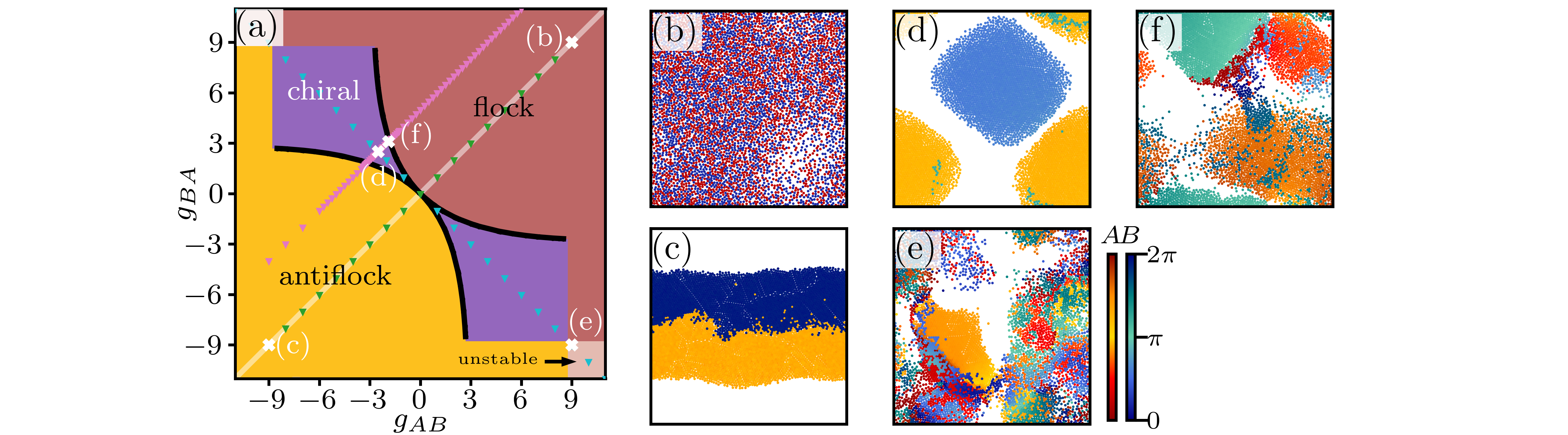
Figure 1: Stability diagram of the homogeneous flocking and antiflocking states against infinite-wavelength perturbations and particle simulation snapshots. The stability diagram in (a) is obtained from linear stability analyses of the continuum Eqs. (4) and (5) for different interspecies coupling strengths $g_{AB}$ and $g_{BA}$. The intraspecies coupling strength is set to $g_{AA}=g_{BB}=9$. Exceptional points are indicated as black lines. The reciprocal system is marked with a white line. Green, cyan, and pink triangles denote data points corresponding to the particle simulations discussed in Figs. 2, 3, and 4, respectively. The Brownian Dynamics simulation snapshots correspond to (b) $g_{AB}=g_{BA}=9$, (c) $g_{AB}=g_{BA}=-9$, (d) $g_{AB}=-g_{BA}=-2.5$, (e) $g_{AB}=-g_{BA}=9$, and (f) $g_{AB}=g_{BA}-5=-1.9$. The color code in (f) indicates the particle type and orientation. Other parameters are specified in text. The stability diagram and snapshots are consistent with Ref. Kreienkamp and Klapp (2025).

II.1.2 Continuum description

The main characteristics of the collective behavior of particles can be captured on a mean-field continuum level. The continuum model is coarse-grained from the microscopic model (1a) and (1b) Kreienkamp and Klapp (2022, 2024b, 2024a, 2025). The deterministic continuum model consists of time evolution equations for the density fields $\rho^{a}(\bm{r},t)$,

$$\partial_{t}\rho^{a}=-\nabla\cdot\big(v^{\rm eff}(\rho)\,\bm{w}^{a}-D_{\rm t}\,\nabla\,\rho^{a}\big),$$ (4)

and polarization densities $\bm{w}^{a}(\bm{r},t)$,

$$\partial_{t}\bm{w}^{a}=\bm{\mathcal{F}}^{a}[\rho^{a},\rho^{b},\bm{w}^{a},\bm{w}^{b}],$$ (5)

of species $a=A,B$, where $b\neq a$ and

$$\begin{split}\bm{\mathcal{F}}^{a}[\rho^{a},\rho^{b},&\bm{w}^{a},\bm{w}^{b}]=\sum_{b}g^{\prime}_{ab}\,\rho^{a}\,\bm{w}^{b}-\sum_{b,c}\frac{g^{\prime}_{ab}\,g^{\prime}_{ac}}{2\,D_{\rm r}}\,\bm{w}^{a}\,(\bm{w}^{b}\cdot\bm{w}^{c})-D_{\rm r}\,\bm{w}^{a}+\mathcal{O}(\nabla\cdot\bm{w})+\mathcal{O}(\nabla\rho).\end{split}$$ (6)

The polarization density measures the overall orientation at a certain position via $\bm{w}^{a}/\rho^{a}$. In the continuum description, the effect of steric repulsion is captured by the effective density-dependent velocity $v^{\rm eff}(\rho)={\rm Pe}-z\,\rho$ with $\rho=\sum_{b}\rho^{b}$, describing the slowing down of particles in crowded situations. The full functional $\bm{\mathcal{F}}^{a}$ is given in Eq. (44) in Appendix A.

In the strong-coupling regime, i.e., for $g>4\,D_{\rm r}/(R_{\theta}^{2}\,\rho_{0})$, a linear stability analysis of the homogeneous flocking and antiflocking states with respect to infinite-wavelength perturbations in the mean-field continuum Eqs. (4) and (5) yields the stability diagram shown in Fig. 1(a). The ‘chiral’ state corresponds to a state, where flocking and antiflocking are predicted to be stable. Further details of the linear stability analysis can be found in Ref. Kreienkamp and Klapp (2025).

II.1.3 Exceptional points in continuum model

In the present study, we are interested in the entropy production rate in the strong-coupling regime, where the dynamics are dominated by polarization. In particular, we focus on the chiral states and the transition to these states. In the continuum description, these transitions are marked by so-called exceptional points Fruchart et al. (2021). Generally, EPs arise in non-Hermitian field theories – including non-reciprocal field theories – and correspond to parameter values where two eigenvalues of the linear stability matrix coalesce and their eigenvectors become parallel El-Ganainy et al. (2018); You et al. (2020); Fruchart et al. (2021); Suchanek et al. (2023c).

In our system, we focus on so-called critical EPs separating the chiral states from flocking and antiflocking states, as seen in the linear stability diagram in Fig. 1. They occur via the coalescence of a damped flocking (or antiflocking) mode with a Goldstone mode and appear only for infinite-wavelength perturbations to the homogeneous flocking and antiflocking states. A detailed analysis of these EPs in the mean-field continuum model can be found in Refs. Fruchart et al. (2021); Kreienkamp and Klapp (2025).

In Secs. B and II.3, we first examine the entropy production rate at the microscopic (particle) level, demonstrating that these field-theoretical EPs – recently linked to enhanced rotational motion of particles Kreienkamp and Klapp (2025) – also manifest in the entropy production rate of particles. In Sec. II.4, we then return to the continuum framework to derive an analytical expression for the entropy production rate at the field level.

II.2 Framework for the entropy production rate on microscopic level

The general framework to calculate the entropy production rate of active particles is based on the formalism of stochastic thermodynamics Seifert (2005, 2012); Dabelow et al. (2019); Fodor et al. (2022). Here, we focus on the steady-state entropy production rate, defined as the time-averaged mean

$$\langle\Delta\dot{S}\rangle=\lim_{\tau\rightarrow\infty}\Delta S[\vec{\bm{\varphi}}]/\tau,$$ (7)

where $\Delta S[\vec{\bm{\varphi}}]$ is the medium entropy production associated with the fluctuating trajectory $\vec{\bm{\varphi}}$. In the context of active matter, the quantity $\langle\Delta\dot{S}\rangle$ is referred to as the informatic entropy production rate Seifert (2012); Nardini et al. (2017); it serves as a measure of the system’s distance from equilibrium Fodor et al. (2022).

Generally, a system’s total entropy production can be decomposed into the system entropy production, associated with the system degrees of freedom, and the medium entropy production $\Delta S$, which measures the entropy produced in the environment. While the system entropy production captures the configurational changes in the system and vanishes in the non-equilibrium steady state considered here, the medium entropy production is expected to be non-zero. To calculate this quantity, we choose a trajectory that starts at a fixed $\bm{\varphi}(t_{0})=\bm{\varphi}_{0}$ and ends at the final $\bm{\varphi}(\tau)=\bm{\varphi}_{\tau}$. The medium entropy production is then given by the log-ratio of the forward path probability $\mathfrak{p}[\vec{\bm{\varphi}}_{\backslash t_{0}}|\bm{\varphi}(t_{0})]$ and the backward path probability $\mathfrak{p^{\dagger}}[\vec{\bm{\varphi}}^{\dagger}_{\backslash t_{0}}|\bm{\epsilon}\,\bm{\varphi}(\tau)]$ Seifert (2005, 2008); Spinney and Ford (2012); Crosato et al. (2019),

$$\Delta S[\vec{\bm{\varphi}}]=k_{\rm B}\,{\rm ln}\left(\frac{\mathfrak{p}[\vec{\bm{\varphi}}_{\backslash t_{0}}|\bm{\varphi}(t_{0})]}{\mathfrak{p^{\dagger}}[\vec{\bm{\varphi}}^{\dagger}_{\backslash t_{0}}|\bm{\epsilon}\,\bm{\varphi}(\tau)]}\right)$$ (8)

with Boltzmann constant $k_{\rm B}$. The forward path probability quantifies the probability for the trajectory $\vec{\bm{\varphi}}_{\backslash t_{0}}=\{\bm{\varphi}(t)|t\in(t_{0},\tau]\}$, which does not include the initial point $\bm{\varphi}_{0}$. The backward path probability is the probability of observing the time reverse of trajectory $\vec{\bm{\varphi}}_{\backslash t_{0}}$, defined as $\vec{\bm{\varphi}}_{\backslash t_{0}}^{\dagger}=\{\bm{\varphi}^{\dagger}|t\in(t_{0},\tau]\}$ with $\bm{\varphi}^{\dagger}(t)=\bm{\epsilon}\,\bm{\varphi}(\tau+t_{0}-t)$. The time reversal operation $\bm{\epsilon}\bm{\varphi}=(\epsilon_{1}\,\varphi_{1},...,\epsilon_{n}\,\varphi_{n})$ distinguishes between variables that are even or odd under time reversal Spinney and Ford (2012). For translational variables (like positions or velocities), $\varphi_{i}$ even implies $\epsilon_{i}\,\varphi_{i}=\varphi_{i}$ and $\varphi_{i}$ odd implies $\epsilon_{i}\,\varphi_{i}=-\varphi_{i}$. For rotational variables (like orientations), $\varphi_{i}$ even implies $\epsilon_{i}\,\varphi_{i}=\varphi_{i}$, and $\varphi_{i}$ odd implies $\epsilon_{i}\,\varphi_{i}=\varphi_{i}+\pi$ Crosato et al. (2019). Generally, the probability measure $\mathfrak{p^{\dagger}}$ for time-reversed path may differ from $\mathfrak{p}$, since it takes into account the time-reversal operation on protocol variables, like, e.g., (odd) external magnetic fields. However, in our model, all parameters are time-independent and even under time-reversal, such that $\mathfrak{p^{\dagger}}[\cdot]=\mathfrak{p}[\cdot]$ Crosato et al. (2019).

Following Refs. Spinney and Ford (2012); Crosato et al. (2019), the medium entropy production can be linked to the microscopic Langevin dynamics of a system by identifying reversible and irreversible components, see Appendix B.

Which components are reversible or irreversible depends on the choice of the time reversal operator $\bm{\epsilon}$. For the translational degree of freedom, the time reversal operator is unambiguously given by

$$\bm{\epsilon}_{\bm{r}_{i}}\,\bm{r}_{i}=\bm{r}_{i}\quad\text{and}\quad\bm{\epsilon}_{\dot{\bm{r}}_{i}}\,\dot{\bm{r}}_{i}=-\dot{\bm{r}}_{i},$$ (9)

since particle positions remain unchanged under time-reversal, while velocities reverse direction. However, the interpretation of $\bm{\epsilon}$ for the active forcing, which is associated with the self-propulsion in direction $\bm{p}_{i}=(\cos\theta_{i},\sin\theta_{i})$, is less clear.

If the direction of motion is considered to be a result of a physical asymmetry of the particles themselves, it has been argued that self-propulsion should be even under time reversal (with $\epsilon_{\theta_{i}}\,\theta_{i}=\theta_{i}$) Shankar and Marchetti (2018). Contrary, it has also been argued that self-propulsion should be odd when the particles themselves are active, and even when particles move due to external forces, such as passive particles in an active bath Dabelow et al. (2019). Importantly, however, in the absence of steric repulsion ($\bm{F}_{\rm rep}=\bm{0}$) and without translational noise ($D^{\prime}_{\rm t}=0$), the self-propulsion direction $\bm{p}_{i}$ is must be odd under time reversal. In this case, $v_{0}\,\bm{p}_{i}$ represents a physical velocity, which reverses under time reversal Ferretti et al. (2022); Borthne et al. (2020). If $\bm{p}_{i}$ were incorrectly treated as even in this limit, the backward path would have zero probability, resulting in a diverging entropy production.

To avoid these issues in the deterministic limit, we adopt the odd interpretation of active forcing with

$$\epsilon_{\theta_{i}}\,\theta_{i}=\theta_{i}+\pi,\quad\epsilon_{\dot{\theta}_{i}}\,\dot{\theta}_{i}=-\dot{\theta}_{i},\quad\bm{\epsilon}_{\bm{p}_{i}}\,\bm{p}_{i}=-\bm{p}_{i}.$$ (10)

Applying this entropy production framework to the specific case of a non-reciprocal polar active mixture governed by the overdamped Langevin equations (1a) and (1b), as shown in Appendix B, we see that the total informatic entropy production rate of particle $\alpha$ naturally splits into two parts,

$$\langle\Delta\dot{S}_{\alpha}\rangle=\langle\Delta\dot{S}_{\alpha}^{{\rm trans}}\rangle+\langle\Delta\dot{S}_{\alpha}^{{\rm align}}\rangle,$$ (11)

where $\langle\cdot\rangle$ denotes a noise and time average. The contribution from translational motion is given by

$$\begin{split}\langle\Delta\dot{S}_{\alpha}^{{\rm trans}}\rangle=\,&\frac{{k_{\rm B}}}{D^{\prime}_{\rm t}}\Big\langle\Big(\mu_{r}\sum_{\beta\neq\alpha}\bm{F}^{\alpha}_{\rm rep}(\bm{r}_{\alpha},\bm{r}_{\beta})\Big)\circ\dot{\bm{r}}_{\alpha}-(v_{0}\,\bm{p}_{\alpha})\cdot\Big(\sum_{\beta\neq\alpha}\bm{F}^{\alpha}_{\rm rep}(\bm{r}_{\alpha},\bm{r}_{\beta})\Big)\Big\rangle.\end{split}$$ (12)

The contribution from the alignment couplings is

$$\langle\Delta\dot{S}_{\alpha}^{{\rm align}}\rangle=\frac{k_{\rm B}}{D^{\prime}_{\rm r}}\Big\langle\Big(\mu_{\theta}\sum_{\beta\neq\alpha}\mathcal{T}_{\rm al}^{\alpha}(\bm{r}_{\alpha},\bm{r}_{\beta},\theta_{\alpha},\theta_{\beta})\Big)\circ\dot{\theta}_{\alpha}\Big\rangle.$$ (13)

Finally, the total informatic entropy production of all particles of species $a$ is given by the sum over all individual particle contributions,

$$\langle\Delta\dot{S}_{a}\rangle=\sum_{\alpha}\langle\Delta\dot{S}_{\alpha}\rangle.$$ (14)

It is important to note that, in systems where the Langevin equations are coarse-grained or effective descriptions and do no capture all dissipative degrees of freedom, the entropy production in Eq. (14) represents only an apparent entropy production. Further, in overdamped models, some contributions are hidden and only become apparent in underdamped systems Shankar and Marchetti (2018). Recent works have developed thermodynamically consistent formulations based on microscopic Markov jump processes of non-reciprocally interacting particles Mohite and Rieger (2025) and lattice systems with flocking dynamics Proesmans et al. (2025). Nevertheless, the informatic entropy production rate computed from overdamped microscopic models provides a lower bound on the total entropy production and serves as a meaningful measure of irreversibility in the system.

II.3 Numerical results for the entropy production rate on microscopic level

To actually calculate the microscopic informatic entropy production rate, we use results of BD simulations. Our main interest lies in the entropy production in chiral states and EPs, which indicate the transitions to chiral states in the “strong-interspecies-coupling” regime. To this end, we fix the intra-species alignment strength at $g=9$, which satisfies the condition $g>4\,D_{\rm r}/(R_{\theta}^{2}\,\rho_{0})$. This ensures the emergence of non-zero polarization regardless of the values of $g_{AB}$ and $g_{BA}$. The detailed dynamical behavior in this strong-coupling regime is discussed in Ref. Kreienkamp and Klapp (2025).

Here, we characterize the collective particle behavior using two observables, which turn out to be closely related to the entropy production rate: the susceptibility $\chi=N\,{\rm Var}(P)$, which quantifies temporal fluctuations of the global polarization order parameter $P$ via its variance ${\rm Var}(P)$, and the spontaneous chirality $|\Omega_{\rm s}^{i}(t)|$, defined as an average angular frequency that measures the system’s collective rotational motion. The explicit definitions of these microscopic observables, which we calculate for both species separately as well as combined, are provided in Appendix D.

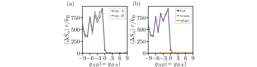
Figure 2: Particle-averaged entropy production rates from particle simulations of a reciprocal system with $g_{AB}=g_{BA}=\kappa$. In (a), the entropy production rate is shown as a function of $g_{AB}$ separately for each particle species, while in (b) the contributions from translational motion and alignment couplings are plotted separately. Other parameters are as specified in Sec. II.1.

II.3.1 Reciprocal reference case

We first consider the reciprocal system with $g_{AB}=g_{BA}=\kappa$ as a reference case. The reciprocal system exhibits flocking for $\kappa>0$ [snapshot in Fig. 1(b)] and antiflocking for $\kappa<0$ [snapshot in Fig. 1(c)]. These states share key characteristics with those in the weak-intraspecies-coupling regime with $g=3<4\,D_{\rm r}/(R_{\theta}^{2}\,\rho_{0})$, studied in detail in Ref. Kreienkamp and Klapp (2024b).

The particle-averaged informatic entropy production rate $\langle\Delta\dot{S}_{\alpha}\rangle$ is shown as a function of $\kappa$ for each species in Fig. 2(a). As expected in a reciprocal system, $\langle\Delta\dot{S}_{\alpha}\rangle$ is nearly identical for both species $A$ and $B$. However, the magnitude of entropy production rate differs significantly between the flocking and antiflocking regimes.

In the antiflocking regime, the informatic entropy production rate is clearly larger than zero, $\langle\Delta\dot{S}_{\alpha}\rangle>300\,k_{\rm B}\,\tau^{-1}$. In contrast, in the flocking regime, it is very small, $\langle\Delta\dot{S}_{\alpha}\rangle<10\,k_{\rm B}\,\tau^{-1}$. This (nearly) vanishing entropy production rate within the flocking state is consistent with previous results for underdamped repulsive polar particles Crosato et al. (2019), overdamped non-repulsive polar particles Ferretti et al. (2022), and active spins in the active Ising model Yu and Tu (2022) .

The decomposition of the entropy production rate into translational alignment contributions is plotted in Fig. 2(b). In the antiflocking regime, the entropy production rate is dominated by the translational contribution, while the alignment contribution remains negligible in both regimes.

This can be understood by analyzing the nature of collective motion and the definitions of translational [Eq. (12)] and alignment [Eq. (13)] contributions to the entropy production rate. In both the flocking and antiflocking regimes, particle orientations change little over time, i.e., $\dot{\theta}_{\alpha}\approx 0$, leading to $\langle\Delta\dot{S}_{\alpha}^{{\rm align}}\rangle\approx 0$. The translational contribution $\langle\Delta\dot{S}_{\alpha}^{{\rm trans}}\rangle$ depends on the steric repulsion force $\bm{F}_{\rm rep}^{\alpha}$ between particles, and is non-zero only when $\bm{F}_{\rm rep}^{\alpha}\neq\bm{0}$.

As seen in the snapshots in Fig. 1(b) and (c), in the flocking state, particles move nearly unhindered in the same direction, without much repulsive interactions, resulting in $\langle\Delta\dot{S}_{\alpha}^{{\rm trans}}\rangle\approx 0$. In contrast, in the antiflocking state, oppositely moving flocks collide. The resulting flocks slide in direction parallel to species interface with frequent collisions between different particles at the interface, leading to $\langle\Delta\dot{S}_{\alpha}^{{\rm trans}}\rangle>0$.

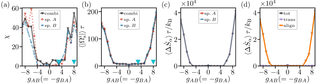
Figure 3: Particle simulation results for a non-reciprocal anti-symmetric system with $g_{AB}=-g_{BA}=\delta$. The (a) susceptibility, (b) spontaneous chirality, and (c),(d) particle-averaged entropy production rates are shown as functions of $g_{AB}$. The parameter values corresponding to the snapshots in Fig. 1(d) and (e) are indicated by cyan markers in (a),(b). In (c), the entropy production rate is shown separately for both particle species, while in (d) the contributions from translational motion and alignment couplings are plotted separately. Other parameters are as specified in Sec. II.1. The susceptibility and spontaneous chirality are consistent with Ref. Kreienkamp and Klapp (2025).

II.3.2 Non-reciprocal anti-symmetric system

We now turn to a non-reciprocal system with anti-symmetric couplings, $g_{AB}=-g_{BA}=\delta$. Here, particles of different species have opposing alignment goals: for $\delta>0$, $A$ wants to align with $B$-particles, while $B$-particles want to antialign with $A$-particles (and the other way round for $\delta<0$). A small (large) value of $|\delta|$ corresponds to a small (strong) degree of non-reciprocity. From a field-theoretical perspective, upon varying $\delta$ one does not cross any exceptional points. Instead, the system remains in the so-called chiral state. Microscopically, the anti-symmetric system exhibits two qualitatively distinct dynamical regimes [see also Ref. Kreienkamp and Klapp (2025)].

For weak anti-symmetric couplings with $|\delta|\lesssim 5$, an almost fully demixed configuration emerges, in which each species forms a large, rotating, synchronized cluster [see snapshot in Fig. 1(d)]. Within each cluster, particles move collectively in nearly constant direction until encountering the cluster of the other species, triggering reorientation and resulting in global rotational motion. Although the susceptibility $\chi(P_{\rm combi})$ of the combined polarization slightly increases with $\delta$ [Fig. 3(a)], the single-species susceptibilities, $\chi(P_{A})$ and $\chi(P_{B})$, as well as spontaneous chirality $\langle|\Omega_{\rm s}^{i}|\rangle$ [Fig. 3(b)] remain relatively small for $|\delta|\lesssim 5$. In this regime, we see that the resulting entropy production rate remains very small with $\langle\Delta\dot{S}_{\alpha}\rangle<50\,k_{\rm B}\,\tau^{-1}$ for $\delta\neq 0$ [Fig. 3(c)] despite the presence of non-reciprocal couplings.

For stronger non-reciprocity ($|\delta|\gtrsim 5$), partially synchronized “chimera-like” states emerge. A representative snapshot of such a state is shown in Fig. 1(e). In this regime, the susceptibilities and the spontaneous chirality grow significantly with $|\delta|$. For example, at $|\delta|=8$, one observes single-species and combined susceptibilities $\chi(P)>40$ and spontaneous chiralities $\langle|\Omega_{\rm s}^{i}|\rangle>125\,\tau^{-1}$. The informatic entropy production rate follows this trend: it increases substantially with the degree of non-reciprocity. For instance, at $|\delta|=8$, one finds $\langle\Delta\dot{S}_{\alpha}\rangle>2.3\cdot 10^{4}\,k_{\rm B}\,\tau^{-1}$.

Despite the coupling asymmetry, the average informatic entropy production rate $\langle\dot{S}_{\alpha}\rangle$ per particles, shown in Fig. 3(c), does not differ significantly between species.

Thus, in the anti-symmetric regime, the informatic entropy production rate mirrors the trends of both the susceptibility and spontaneous chirality. A pronounced effect of non-reciprocity on the entropy production rate (as compared to the reciprocal reference case) arises only for sufficiently large degrees of non-reciprocity, where the strength of interspecies couplings is comparable to intraspecies alignment.

The decomposition of the entropy production rate [Fig. 3(d)] reveals that, in both regimes of the anti-symmetric system, the informatic entropy production rate is almost entirely due to the orientational couplings, with negligible contribution from translational motion. This observation can be explained by the nature of the collective particle motion, seen in the snapshots in Figs. 1(d),(e).

In the regime of large, rotating clusters [Fig. 1(d)], particles of each species form flocks that move coherently until colliding with the other species’ cluster. Similar to reciprocal flocking, the translational contribution remains small due to the lack of significant repulsion, i.e., $\bm{F}_{\rm rep}^{\alpha}\approx 0$. Although the clusters do rotate, spontaneous chirality, and thus $\dot{\theta}$, remains small, keeping the alignment contribution low, too.

In contrast, in the chimera-like state at $|\delta|\gtrsim 5$ [Fig. 1(e)], particles remain relatively loosely distributed, and thus the translational contribution to the entropy production rate remains small, though slightly larger than at smaller $|\delta|$. However, the alignment contribution increases significantly due to rapid orientation changes ($\dot{\theta}^{\alpha}$) and stronger torques ($\mathcal{T}_{\rm al}^{\alpha}$) sustaining the rotational motion.

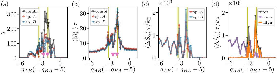
Figure 4: Particle simulation results for a non-reciprocal system with $g_{AB}=g_{BA}-5$. The (a) susceptibility, (b) spontaneous chirality, and (c),(d) particle-averaged entropy production rates are shown as functions of $g_{AB}$. The parameter values corresponding to the snapshots in Fig. 1(d) and (e) are indicated by pink markers in (a),(b). In (c), the entropy production rate is shown separately for both particle species, while in (d) the contributions from translational motion and alignment couplings are plotted separately. Other parameters are as specified in Sec. II.1. The susceptibility and spontaneous chirality are consistent with Ref. Kreienkamp and Klapp (2025).

II.3.3 Non-reciprocal system crossing exceptional points

We now consider non-reciprocal systems with couplings $g_{AB}=g_{BA}-d$, where $d\neq 0$ is fixed. Varying $g_{AB}$ in such systems leads to two crossings of exceptional points in the corresponding mean-field continuum description, which indicate the transition to the chiral state. We denote these points by $g_{AB}^{{\rm EP}>}(d)$ and $g_{AB}^{{\rm EP}<}(d)$, whereby $g_{AB}^{{\rm EP}<}(d)<g_{AB}^{{\rm EP}>}(d)$. Their locations depend on the offset parameter $d$.

In Fig. 4 the susceptibility, spontaneous chirality, and entropy production rate are plotted as functions of $g_{AB}$ for $d=5$. The qualitative behavior remains similar for other values of $d$ (see Appendix E).

For $g_{AB}<-5$, the system is in an antiflocking state, similar to the reciprocal case shown in snapshot Fig. 1(c). For $g_{AB}>0$, the system is in a flocking state, resembling the reciprocal case shown in snapshot Fig. 1(b). In both these limiting states, the susceptibility and spontaneous chirality remain low. As expected, the resulting entropy production rate closely matches that of the corresponding reciprocal systems (see Fig. 2).

Between these two limiting states, the system crosses the exceptional points, which mark qualitative changes in the dynamical behavior, twice. This becomes evident in the snapshots in Fig. 1(d),(f): while large, rotating clusters exist anti-symmetric couplings [$g_{AB}=-g_{BA}=-2.5$ in Fig. 1(d)], these structures break down near the exceptional points [$g_{AB}=-g_{BA}=-1.9$ in Fig. 1(f)], where synchronization weakens, fluctuations of polarizations increase, and clusters dynamically form and dissolve. The dynamical behavior near exceptional points is further discussed in Ref. Kreienkamp and Klapp (2025).

The transition is reflected in the all considered particle-level observables. Near the exceptional points, both the susceptibility and the spontaneous chirality display clear peaks – more pronounced at $g_{AB}^{\rm EP>}$, closer to the flocking regime, than at $g_{AB}^{\rm EP<}$. For instance, at $g_{AB}^{\rm EP>}=-1.9$, we find $\chi>200$ and $\langle|\Omega_{\rm s}^{i}|\rangle>25\,\tau^{-1}$. These values significantly exceed the values for the anti-symmetric system with large, rotating clusters (where $\chi<10$ and $\langle|\Omega_{\rm s}^{i}|\rangle>15\,\tau^{-1}$ at $g_{AB}=-2.5$).

Importantly, in the vicinity of the exceptional points, also the total entropy production rate exhibits pronounced peaks. These peaks are most clearly visible in the orientation-related contribution [Fig. 4(d)], which shows sharp maxima close to the positions of exceptional points identified in the continuum theory. Between these exceptional points, i.e., for intermediate anti-symmetric couplings, the entropy production rate decreases substantially.

Thus, the positions of peaks and minima in the entropy production rate coincide with those of the susceptibility and spontaneous chirality. Furthermore, the peak heights also show qualitative agreement: both entropy production rate and susceptibility attain higher maxima at the exceptional point $g_{AB}^{\rm EP>}$ closer to the flocking regime.

II.4 Entropy production rate in field theory

To substantiate the peaks in the entropy production rate at coupling strengths associated with exceptional points, we now turn to the continuum description of the system.

II.4.1 Fluctuating hydrodynamic model for polarization perturbations

At the continuum level, we calculate the entropy production rate based on path probabilities, which requires considering stochastic fields instead of deterministic ones (that were considered in Sec. II.1.2). The fluctuating hydrodynamic equations include both the deterministic contributions, obtained through coarse-graining, and additional noise terms that are added “by hand” Marchetti et al. (2013); Nardini et al. (2017); Toner et al. (2005); Borthne et al. (2020); Dadhichi et al. (2018). The full fluctuating hydrodynamic equations are given in Appendix G.

For the analytical calculation below, we focus on the time evolution of small perturbations $\bm{w}^{\prime a}$ around stationary solutions $\bm{w}^{a}_{0}$ of the deterministic continuum Eqs. (4) and (5). By focusing on the entropy production rate arising from polarization perturbations (instead of the entropy production rate of the total polarization) we are in the position to obtain analytical results. Further, we specialize on the infinite-wavelength limit with wavenumber $k=0$, where exceptional points are predicted to occur. Due to number conservation, density fluctuations vanish at $k=0$. Hence, we restrict our analysis to the polarization perturbation dynamics alone. To linear order, the mean-field polarization perturbation dynamics for species $a$ at $k=0$ is given by

$$\partial_{t}\bm{w}^{\prime a}=\bm{\mathcal{F}}^{a}_{k=0,{\rm lin}}[\bm{w}^{\prime a},\bm{w}^{\prime b}]+\tilde{\bm{\eta}}_{a},$$ (15)

where $b\neq a$, and both $\bm{w}^{\prime a}=\bm{w}^{\prime a}(t)$, $\tilde{\bm{\eta}}_{a}=\tilde{\bm{\eta}}_{a}(t)$ are homogeneous in space. For stationary solutions of the form $\bm{w}^{a}_{0}=(w_{0}^{a},0)^{\rm T}$, the deterministic contribution is described by the functional

$$\begin{split}\bm{\mathcal{F}}^{a}_{k=0,{\rm lin}}[\bm{w}^{\prime a},\bm{w}^{\prime b}]=\bm{\gamma}^{a}_{a}[w_{0}^{a},w_{0}^{b}]\cdot\bm{w}^{\prime a}+\bm{\gamma}^{a}_{b}[w_{0}^{a},w_{0}^{b}]\cdot\bm{w}^{\prime b}.\end{split}$$ (16)

The prefactors $\bm{\gamma}_{a}^{a}$ and $\bm{\gamma}_{b}^{a}$ can be calculated analytically and are plotted as functions of $g_{AB}$ in Fig. 7 in Appendix F. The alignment strength at the continuum level is given by $g^{\prime}_{ab}=g_{ab}\,R_{\theta}^{2}\,\rho_{0}^{b}/2$. The noise term $\tilde{\bm{\eta}}_{a}$ in Eq. (15) is of strength $D_{\rm h}$, has zero mean, and satisfies

$$\langle\tilde{\eta}_{a,i}(t)\,\tilde{\eta}_{b,j}(t^{\prime})\rangle=2\,D_{\rm h}\,\delta_{ab}\,\delta_{ij}\,\delta(t-t^{\prime}).$$ (17)

II.4.2 Dynamical action

We begin by considering the total entropy production from polarization perturbations, defined as the log-ratio of forward ($\mathfrak{p}[\vec{\bm{w}}^{\prime}]$) and backward ($\mathfrak{p}[\vec{\bm{w}}^{\prime\dagger}]$) path probabilities Seifert (2005); Borthne et al. (2020); Dadhichi et al. (2018),

$$\Delta S[\vec{\bm{w}}^{\prime}]=k_{\rm B}\,{\rm ln}\left(\frac{\mathfrak{p}[\vec{\bm{w}}^{\prime}]}{\mathfrak{p}[\vec{\bm{w}}^{\prime\dagger}]}\right),$$ (18)

for the trajectory $\vec{\bm{w}}^{\prime}=\{(\bm{w}^{\prime A}(t),\bm{w}^{\prime B}(t))|t\in[t_{0},\tau]\}$.

The expression for the probability of individual trajectories in $(\bm{w}^{\prime A},\bm{w}^{\prime B})$-space is provided by the standard Onsager-Machlup path integral Onsager and Machlup (1953); Nardini et al. (2017)

$$\mathfrak{p}[\vec{\bm{w}}^{\prime}]\propto{\rm exp}(-\mathcal{A}[\vec{\bm{w}}^{\prime}])$$ (19)

with dynamical action $\mathcal{A}[\vec{\bm{w}}^{\prime}]$.

For our binary mixture at $k=0$, the total dynamical action includes contributions from $\bm{w}^{\prime A}$ and $\bm{w}^{\prime B}$, such that

$$\mathcal{A}[\vec{\bm{w}}^{\prime}]=\mathcal{A}_{\bm{w}^{\prime A}}+\mathcal{A}_{\bm{w}^{\prime B}}.$$ (20)

In the $k=0$-limit, the contribution from species $a=A,B$ takes the form

$$\begin{split}\mathcal{A}_{\bm{w}^{\prime a}}=&\frac{1}{4\,D_{\rm h}}\iint\big(\partial_{t}\bm{w}^{\prime a}-\bm{\mathcal{F}}^{a}_{k=0,{\rm lin}}[\bm{w}^{\prime a},\bm{w}^{\prime b}]\big)^{2}\,{\rm d}\bm{r}\,{\rm d}t+\mathcal{A}_{\bm{w}^{\prime a}}^{\rm conv},\end{split}$$ (21)

where

$$\mathcal{A}_{\bm{w}^{\prime a}}^{\rm conv}=\frac{1}{2}\,\iint\frac{\delta\bm{\mathcal{F}}^{a}_{k=0,{\rm lin}}[\bm{w}^{\prime a},\bm{w}^{\prime b}]}{\delta\bm{w}^{\prime a}}\,{\rm d}\bm{r}\,{\rm d}t$$ (22)

accounts for the convention-dependent contributions to the dynamics due to the discretization scheme with respect to noise. Here, we use Stratonovich (midpoint) discretization.

II.4.3 Backwards probability

In addition to the forward path probability (19), we also require the probability for the time-reversed backward path, given by

$$\mathfrak{p}[\vec{\bm{w}}^{\prime\dagger}]\propto{\rm exp}(-\mathcal{A}[\vec{\bm{w}}^{\prime\dagger}])={\rm exp}(-\overleftarrow{\mathcal{A}}_{\bm{w}^{\prime A}}+\overleftarrow{\mathcal{A}}_{\bm{w}^{\prime B}}),$$ (23)

which measures the probability of observing the trajectory $\vec{\bm{w}}^{\prime\dagger}$ under the same forward time evolution equation (15). For Stratonovich convention, the normalization factors for forward and backward path probabilities in Eqs. (19) and (23) are identical Cates et al. (2022); Cugliandolo and Lecomte (2017).

To define the backward path, we must specify a time-reversal protocol. Consistent with our particle-level considerations, we impose a polarity flip under time reversal, such that

$$\bm{w}^{\prime a\dagger}(\bm{r},t)=-\bm{w}^{\prime a}(\bm{r},\tau+t_{0}-t).$$ (24)

This polarity flip is indeed necessary when the density dynamics are purely deterministic Borthne et al. (2020).

The $a$-species action of the time-reversed trajectory is

$$\begin{split}\overleftarrow{\mathcal{A}}_{\bm{w}^{\prime a}}=&\frac{1}{4\,D_{\rm h}}\iint\big(\partial_{t}\bm{w}^{\prime a\dagger}-\bm{\mathcal{F}}^{a}_{k=0,{\rm lin}}[\bm{w}^{\prime a\dagger},\bm{w}^{\prime b\dagger}]\big)^{2}\,{\rm d}\bm{r}\,{\rm d}t+\overleftarrow{\mathcal{A}}_{\bm{w}^{\prime a}}^{\rm conv}\end{split}$$ (25)

with

$$\overleftarrow{\mathcal{A}}_{\bm{w}^{\prime a}}^{\rm conv}=\frac{1}{2}\,\iint\frac{\delta\bm{\mathcal{F}}^{a}_{k=0,{\rm lin}}[\bm{w}^{\prime a\dagger},\bm{w}^{\prime b\dagger}]}{\delta\bm{w}^{\prime a\dagger}}\,{\rm d}\bm{r}\,{\rm d}t.$$ (26)

The functional $\bm{\mathcal{F}}^{a}_{k=0}$ is anti-symmetric under time reversal, i.e.,

$$\bm{\mathcal{F}}^{a}_{k=0,{\rm lin}}[\bm{w}^{\prime a\dagger},\bm{w}^{\prime b\dagger}]=-\bm{\mathcal{F}}^{a}_{k=0,{\rm lin}}[\bm{w}^{\prime a},\bm{w}^{\prime b}].$$ (27)

Hence, the action of the time-reversed trajectory, expressed in terms of the forward trajectory, is

$$\begin{split}\overleftarrow{\mathcal{A}}_{\bm{w}^{\prime a}}=&\frac{1}{4\,D_{\rm h}}\iint\big(\partial_{t}\bm{w}^{\prime a}+\bm{\mathcal{F}}^{a}_{k=0,{\rm lin}}[\bm{w}^{\prime a},\bm{w}^{\prime b}]\big)^{2}\,{\rm d}\bm{r}\,{\rm d}t+\mathcal{A}_{\bm{w}^{\prime a}}^{\rm conv}.\end{split}$$ (28)

II.4.4 Entropy production

From Eq. (18), it follows that the entropy production for species $a$ along the trajectory $\vec{\bm{w}}^{\prime}$ is given by

$$\Delta S^{a}=k_{\rm B}\,\big(\overleftarrow{\mathcal{A}}_{\bm{w}^{\prime a}}-\mathcal{A}_{\bm{w}^{\prime a}}\big).$$ (29)

Inserting the expressions (21) and (25) for the actions, we obtain

$$\Delta S^{a}=-\frac{k_{\rm B}}{D_{\rm h}}\iint\big(-(\partial_{t}\bm{w}^{\prime a})\circ\bm{\mathcal{F}}^{a}_{k=0,{\rm lin}}[\bm{w}^{\prime a},\bm{w}^{\prime b}]\big)\,{\rm d}\bm{r}\,{\rm d}t,$$ (30)

where $\circ$ indicates a product interpreted in the Stratonovich sense.

We now compute the entropy production rate $\langle\Delta\dot{S}\rangle=\langle\Delta\dot{S}^{A}\rangle+\langle\Delta\dot{S}^{B}\rangle$ as defined in Eq. (7). To this end, we first split $\bm{\mathcal{F}}^{a}_{k=0,{\rm lin}}$ into a component depending on $\bm{w}^{\prime a}$,

$$\begin{split}&\bm{\mathcal{F}}^{a,\bm{w}^{\prime a}}_{k=0,{\rm lin}}[\bm{w}^{\prime a}]=\bm{\gamma}^{a}_{a}[w_{0}^{a},w_{0}^{b}]\cdot\bm{w}^{\prime a},\end{split}$$ (31)

and one depending on $\bm{w}^{\prime b}$ with $b\neq a$,

$$\begin{split}&\bm{\mathcal{F}}^{a,\bm{w}^{\prime b}}_{k=0,{\rm lin}}[\bm{w}^{\prime b}]=\bm{\gamma}^{a}_{b}[w_{0}^{a},w_{0}^{b}]\cdot\bm{w}^{\prime b}.\end{split}$$ (32)

Accordingly, the entropy production $\Delta S^{a}$ splits into two parts: $\Delta S^{a}=\Delta S^{a}_{1}+\Delta S^{a}_{2}$. Since the integral in Eq. (30) is interpreted in the Stratonovich sense, the (common) chain rule applies. The first part, involving $\bm{\mathcal{F}}^{a,\bm{w}^{\prime a}}_{k=0,{\rm lin}}$, becomes

$$\begin{split}\Delta S^{a}_{1}&=\frac{k_{\rm B}}{D_{\rm h}}\iint(\partial_{t}\bm{w}^{\prime a})\circ\bm{\mathcal{F}}^{a,\bm{w}^{\prime}_{a}}_{k=0,{\rm lin}}[\bm{w}^{\prime a}]\,{\rm d}\bm{r}\,{\rm d}t\\ &=\frac{k_{\rm B}}{D_{\rm h}}\iint\big(\bm{\mathcal{F}}^{a,\bm{w}^{\prime a}}_{k=0,{\rm lin}}[\bm{w}^{\prime a}]\big)\,{\rm d}\bm{r}\,{\rm d}\bm{w}^{\prime a}\\ &=\frac{k_{\rm B}}{D_{\rm h}}\int\left(\frac{\bm{\gamma}^{a}_{a}}{2}\cdot\bm{w}^{\prime a}\right)\cdot\bm{w}^{\prime a}\,{\rm d}\bm{r},\end{split}$$ (33)

where we used direct integration in the last step. For the entropy production rate [Eq. (7)], the term $\Delta S_{1}/\tau\rightarrow 0$ as $\tau\rightarrow\infty$, because all moments of $\bm{w}^{\prime a}$ remain finite in the steady state.

The second part, involving $\bm{\mathcal{F}}^{a,\bm{w}^{\prime b}}_{k=0,{\rm lin}}$, is split into two contributions by inserting Eq. (15) for $\partial_{t}\bm{w}^{\prime a}$,

$$\begin{split}\Delta S^{a}_{2}&=\frac{k_{\rm B}}{D_{\rm h}}\iint(\partial_{t}\bm{w}^{\prime a})\circ\bm{\mathcal{F}}^{a,\bm{w}^{\prime}_{b}}_{k=0,{\rm lin}}[\bm{w}^{\prime b}]\,{\rm d}\bm{r}\,{\rm d}t\\ &=\Delta S^{a}_{2.1}+\Delta S^{a}_{2.2}\end{split}$$ (34)

with

$$\begin{split}\Delta S^{a}_{2.1}=&\frac{k_{\rm B}}{D_{\rm h}}\iint\bm{\mathcal{F}}^{a}_{k=0,{\rm lin}}\cdot\bm{\mathcal{F}}^{a,\bm{w}^{\prime b}}_{k=0,{\rm lin}}{\rm d}\bm{r}\,{\rm d}t\end{split}$$ (35)

and

$$\begin{split}\Delta S^{a}_{2.2}=&\frac{k_{\rm B}}{D_{\rm h}}\iint\tilde{\bm{\eta}}_{a}\circ\bm{\mathcal{F}}^{a,\bm{w}^{\prime b}}_{k=0,{\rm lin}}\,{\rm d}\bm{r}\,{\rm d}t.\end{split}$$ (36)

While $\Delta S_{2.1}$ is noise-independent and directly yields a contribution to the entropy production rate upon division by $\tau$ and taking the limit $\tau\rightarrow\infty$, $\Delta S_{2.2}$ must be calculated explicitly.

To treat the Stratonovich product in Eq. (36), we convert it into an Itô product. The advantage is that in Itô calculus, equal-time correlations like $\langle\tilde{\bm{\eta}}^{a}\cdot\bm{w}^{\prime c}\rangle$ (with $c=a$ or $c\neq a$) vanish Gardiner (1985). The relevant conversions between Stratonovich and Itô are of form Gardiner (1985); Borthne et al. (2020); Cates et al. (2022)

$$\begin{split}\langle h(\bm{w}^{\prime c}(\bm{r},&t))\circ\tilde{\eta}_{a,i}(\bm{r}^{\prime},t)\rangle=\,\langle h(\bm{w}^{\prime c}(\bm{r},t))\cdot\tilde{\eta}_{a,i}(\bm{r}^{\prime},t)\rangle+D_{\rm h}\,\Big\langle\frac{\partial h(\bm{w}^{\prime c}(\bm{r},t))}{\partial w^{\prime b}_{j}(\bm{r}^{\prime},t)}\Big\rangle\,\delta(\bm{r}-\bm{r}^{\prime})\,\delta_{ab}\,\delta_{ij}\end{split}$$ (37)

where $h$ is a function of $\bm{w}^{\prime}$, and $\cdot$ denotes the Itô product . Since the Itô product vanishes in the equal-time expectation, only the conversion contribution, i.e., the second contribution on the r.h.s. of Eq. (37), remains to be evaluated. In our case, $\bm{\mathcal{F}}^{a,\bm{w}^{\prime b}}_{k=0,{\rm lin}}$ is independent of $\bm{w}^{\prime a}$, so also the conversion term vanishes, and hence $\Delta S^{a}_{2.2}=0$.

Therefore, the only contribution to the entropy production rate for polarization fluctuations of species $a$ arises from $\Delta S^{a}_{2.1}$, such that

$$\begin{split}\langle\Delta\dot{S}^{a}\rangle=\frac{k_{\rm B}}{D_{\rm h}}\left\langle\int\bm{\mathcal{F}}^{a}_{k=0,{\rm lin}}\cdot\bm{\mathcal{F}}^{a,\bm{w}^{\prime b}}_{k=0,{\rm lin}}{\rm d}\bm{r}\right\rangle\end{split}$$ (40)

Substituting the explicit forms of $\bm{\mathcal{F}}^{a}_{k=0,{\rm lin}}$ and $\bm{\mathcal{F}}^{a,\bm{w}^{\prime b}}_{k=0,{\rm lin}}$ yields

$$\begin{split}\langle\Delta\dot{S}^{a}\rangle=\frac{k_{\rm B}}{D_{\rm h}}\Big(&\gamma^{a}_{a,\ell}\,\gamma^{a}_{b,\ell}\,\chi_{{\rm f},\ell}^{ab}+(\gamma^{a}_{b,\ell})^{2}\,\chi_{{\rm f},\ell}^{bb}+\gamma^{a}_{a,t}\,\gamma^{a}_{b,t}\,\chi_{{\rm f},t}^{ab}+(\gamma^{a}_{b,t})^{2}\,\chi_{{\rm f},t}^{bb}\Big)\end{split}$$ (41)

with longitudinal and transversal susceptibilities of the polarization fluctuations defined as

$$\chi_{{\rm f},\ell}^{aa}=\left\langle\int w^{\prime a}_{x}\,w^{\prime a}_{x}\,{\rm d}\bm{r}\right\rangle,\ \ \chi_{{\rm f},\ell}^{ab}=\left\langle\int w^{\prime a}_{x}\,w^{\prime b}_{x}\,{\rm d}\bm{r}\right\rangle,$$ (42)

and

$$\chi_{{\rm f},t}^{aa}=\left\langle\int w^{\prime a}_{y}\,w^{\prime a}_{y}\,{\rm d}\bm{r}\right\rangle,\ \ \chi_{{\rm f},t}^{ab}=\left\langle\int w^{\prime a}_{y}\,w^{\prime b}_{y}\,{\rm d}\bm{r}\right\rangle.$$ (43)

In the $k=0$-limit, the field $\bm{w}^{\prime a}=\bm{w}^{\prime a}(t)$ is spatially uniform, so spatial integrals reduce to multiplication by the system size.

The key result, given by Eq. (41), is that, in the infinite-wavelength limit, the entropy production rate of polarization perturbations scales with their susceptibilities. According to the prefactors to the susceptibilities (see Fig. 7 in Appendix F), the longitudinal mixed-species susceptibilities, $\chi^{AB}_{{\rm f},\ell}$ and $\chi^{BA}_{{\rm f},\ell}$, contribute most significantly. However, the transversal and same-species contributions also remain nonzero.

Taken together, we have shown that both the particle and continuum entropy production rates are closely related to orientational susceptibilities. Despite this qualitative agreement, we note that the numerical (particle-based) and analytical (field-theoretical) quantities differ in detail. On the particle level, the entropy production rate behaves similarly to the temporal fluctuations of the global polarization, given by the susceptibility of the scalar polarization order parameter, $\chi=N\,{\rm Var}(P)$. On the other hand, the analytical approach considers $k=0$-perturbations around homogeneous base states, using vectorial perturbations $\bm{w}^{\prime a}=\bm{w}^{a}-\bm{w}^{a}_{0}$. The entropy production at the field level scales with susceptibilities defined through these perturbations, which are not directly accessible on the particle level. Nevertheless, the analytical field-theoretical results provide a qualitative explanation for the observed correlation between susceptibility and informatic entropy production rate on the particle level.

While we focused here only on the contribution of the polarization perturbations alone to the entropy production rate, the analytical calculation of the entropy production rate for the full polarization dynamics in the limit of $k=0$ is presented in Appendix H. To go beyond the infinite-wavelength limit, we also provide the full entropy production rate of the fluctuating hydrodynamic density and polarization density fields [see Eqs. (57)-(59)] in Appendix I. Numerical continuum simulations reveal that the overall dependence of the entropy production rate on the coupling strength resembles the one obtained from particle simulations, including, in particular, the peaks near exceptional points.

III Conclusion

We have studied the informatic entropy production rate at phase transitions associated to non-reciprocity-induced collective behavior in active matter systems. As a measure of distance from equilibrium, the entropy production rate captures the twofold non-equilibrium character arising from both activity and non-reciprocal orientational couplings. Moreover, it reflects phase transitions through pronounced signatures at exceptional points.

Specifically, we have focused on a binary mixture of polar particles, where non-reciprocal orientational couplings lead to spontaneous rotational motion and (partial) synchronization.

As a first main result, our particle simulations demonstrate that non-reciprocal orientational couplings can leave a clear signature in the entropy production rate – also in active systems consisting of self-propelling polar particles. For sufficiently strong non-reciprocal couplings, the informatic entropy production rate increases with the strength of non-reciprocity. However, this is not always the case: when non-reciprocity is weak compared to the intraspecies alignment and the non-reciprocal couplings are anti-symmetric, the entropy production rate remains relatively low – comparable to that of conventional reciprocal flocking states.

However, even in the regime of weak non-reciprocity, the entropy production rate exhibits pronounced peaks when the coupling strengths are not anti-symmetric but correspond to exceptional points in the associated field theory. These findings are consistent with field-theoretical studies of scalar Cahn-Hilliard systems, where transitions to traveling states are also accompanied by peaks in entropy production Suchanek et al. (2023a, b). This suggests that, as in scalar field theories, active polar particle systems exhibit non-trivial entropy production behavior at exceptional points.

Overall, we find, at the particle level, a strong correspondence between the behaviors of the susceptibility, spontaneous chirality and entropy production rate as functions of non-reciprocal couplings.

As the second key result, we substantiate this correspondence through field-theoretical analytical calculations. In the analytically tractable infinite-wavelength limit, we show that the entropy production rate of polarization perturbations scales with their susceptibilities, providing a qualitative explanation for the particle-based findings.

The combination of our particle- and continuum-level results suggests that the susceptibility of the polar order parameter, which could be measured in experiments, can serve as an estimate of the informatic entropy production rate of active particles. Indeed, the entropy production has recently gained importance as a key quantity in optimal control strategies of, e.g., active particles Soriani et al. (2025); Garcia-Millan et al. (2024) or passive particles in complex environments Loos et al. (2024). It is also emerging as an important tool for gaining insight into biological processes Li et al. (2024); Tan et al. (2021); Seifert (2019). An intriguing direction for future research is to explore the connection between entropy production rate and universal scaling behaviors near critical exceptional points Liu et al. (2025).

Appendix A Full deterministic continuum equations

The continuum equation for the particle density is the continuity Eq. (4). The evolution equation for the polarization density, Eq. (5), contains the functional

$$\begin{split}\bm{\mathcal{F}}^{a}[\rho^{a},\rho^{b},\bm{w}^{a},\bm{w}^{b}]=&-\frac{1}{2}\,\nabla\,\big(v^{\rm eff}(\rho)\,\rho^{a}\big)-D_{\rm r}\,\bm{w}^{a}+\sum_{b}g^{\prime}_{ab}\,\rho^{a}\,\bm{w}^{b}+D_{\rm t}\,\nabla^{2}\,\bm{w}^{a}+\frac{v^{\rm eff}(\rho)}{16\,D_{\rm r}}\,\nabla^{2}\,\Big(v^{\rm eff}(\rho)\,\bm{w}^{a}\Big)\\ &-\sum_{b,c}\frac{g^{\prime}_{ab}\,g^{\prime}_{ac}}{2\,D_{\rm r}}\,\bm{w}^{a}\,(\bm{w}^{b}\cdot\bm{w}^{c})-\frac{z}{16\,D_{\rm r}}\,\nabla\rho\cdot\big[\nabla\big(v^{\rm eff}(\rho)\,\bm{w}^{a}\big)-\nabla^{*}\big(v^{\rm eff}(\rho)\,\bm{w}^{a*}\big)\big]\\ &+\sum_{b}\frac{g^{\prime}_{ab}}{8\,D_{\rm r}}\Big[\bm{w}^{b}\cdot\nabla\big(v^{\rm eff}(\rho)\,\bm{w}^{a}\big)+\bm{w}^{b*}\cdot\nabla\big(v^{\rm eff}(\rho)\,\bm{w}^{a*}\big)-2\,\Big\{v^{\rm eff}(\rho)\,\bm{w}^{a}\cdot\nabla\bm{w}^{b}\\ &\qquad+\bm{w}^{b}\,\nabla\cdot\big(v^{\rm eff}(\rho)\,\bm{w}^{a}\big)-v^{\rm eff}(\rho)\,\bm{w}^{a*}\cdot\nabla\bm{w}^{b*}-\bm{w}^{b*}\,\nabla\cdot\big(v^{\rm eff}(\rho)\,\bm{w}^{a*}\big)\Big\}\Big],\end{split}$$ (44)

where $\bm{w}^{*}=(w_{y},-w_{x})^{\rm T}$ and $\nabla^{*}=(\partial_{y},-\partial_{x})^{\rm T}$. The continuum equations are non-dimensionalized using a characteristic time scale $\tau$ and length scale $\ell$. The particle and polarization densities of species $a$ are scaled by the average particle density $\rho_{0}^{a}$. The remaining five dimensionless control parameters are the Péclet number ${\rm Pe}=v_{0}\,\tau/\ell$, $z=\zeta\,\rho^{a}_{0}\,\tau/\ell$ measuring the particle velocity-reduction due to the environment, the translational diffusion coefficient $D_{\rm t}=D^{\prime}_{\rm t}\,\tau/\ell^{2}$, the rotational diffusion coefficient $D_{\rm r}=D^{\prime}_{\rm r}\,\tau$, and the orientational coupling parameter $g^{\prime}_{ab}=k_{ab}\,\mu_{\theta}\,R_{\theta}^{2}\,\rho_{0}^{b}\,\tau/2$. (For the parameters used in this study, the continuum ($g^{\prime}_{ab}$) and particle ($g_{ab}$) orientational coupling parameters are related via $g^{\prime}_{ab}=12.73\,g_{ab}$.)

The continuum parameters are chosen to match the corresponding particle-level parameters. While most of these can be directly adopted, the velocity reduction parameter $z$ needs to be determined from the pair distribution function of particles. As described in Kreienkamp and Klapp (2024b), it is given by $z=\zeta\,\rho^{a}_{0}\,\tau/\ell=57.63\,\rho^{a}_{0}\,\tau/\ell=0.37\,{\rm Pe}/\rho_{0}^{\rm con}$ with $\rho_{0}^{\rm con}=1$. Furthermore, we adopt an ad-hoc choice of $D_{\rm t}=9$ Kreienkamp and Klapp (2024b).

Appendix B Calculation of the entropy production rate on the microscopic level

Following Refs. Spinney and Ford (2012); Crosato et al. (2019), the medium entropy production can be linked to the microscopic Langevin dynamics of a system $\bm{\varphi}=(\phi_{1},...,\phi_{n})$, consisting of $n$ coupled stochastic differential equations of form

$${\rm d}\phi_{i}=A^{\rm rev}_{\phi_{i}}[\bm{\varphi}(t),t]\,{\rm d}t+A^{\rm ir}_{\phi_{i}}[\bm{\varphi}(t),t]\,{\rm d}t+B_{\phi_{i}}\,{\rm d}W_{i},$$ (45)

where $W_{i}$ are Wiener processes with ${\rm d}W_{i}\,{\rm d}W_{j}=\delta_{ij}\,{\rm d}t$ and $B_{\phi_{i}}$ are scalar. The reversible and irreversible components of the deterministic dynamics satisfy Spinney and Ford (2012); Risken and Risken (1996)

$$A^{\rm rev}_{\phi_{i}}[\bm{\varphi}(t),t]=-\epsilon_{\phi_{i}}\,A^{\rm rev}_{\phi_{i}}[\bm{\epsilon}\bm{\varphi}(t),t]$$ (46)

and

$$A^{\rm ir}_{\phi_{i}}[\bm{\varphi}(t),t]=\epsilon_{\phi_{i}}\,A^{\rm ir}_{\phi_{i}}[\bm{\epsilon}\bm{\varphi}(t),t],$$ (47)

where $\epsilon_{\phi_{i}}\in\{-1,+1\}$ for $\phi_{i}$ odd and even, respectively Crosato et al. (2019).

To calculate the entropy production from path probabilities, one considers the Fokker-Planck equation that corresponds to the Langevin equation (45) and its solution, the short time Green’s function or “short time propagator” $\mathfrak{p}(\bm{\varphi}^{\prime},t+{\rm d}t|\bm{\varphi},t)$. The latter is the conditional probability of a displacement $d\bm{\varphi}=\bm{\varphi}^{\prime}-\bm{\varphi}$ in a time ${\rm d}t$ given an initial $\delta$-function. The medium entropy production along the path $\vec{\bm{\varphi}}$ is then given by the path integral Spinney and Ford (2012); Seifert (2005); Crosato et al. (2019)

$$\Delta S[\vec{\bm{\varphi}}]=\int_{t_{0}}^{\tau}{\rm d}\Delta S(t)$$ (48)

with increments

$$\begin{split}{\rm d}\Delta S(t)&=k_{\rm B}\,{\rm ln}\left(\frac{\mathfrak{p}(\bm{\varphi}^{\prime},t+{\rm d}t|\bm{\varphi},t)}{\mathfrak{p}(\bm{\epsilon}\bm{\varphi}^{\prime},t+{\rm d}t|\bm{\epsilon}\bm{\varphi},t)}\right)\\ &=k_{\rm B}\sum_{\phi_{i}\in\bm{\varphi}}\Big(\frac{A^{\rm ir}_{\phi_{i}}(\bm{\varphi}(t))}{D_{\phi_{i}}}\circ{\rm d}\phi_{i}-\frac{A^{\rm ir}_{\phi_{i}}(\bm{\varphi}(t))\,A^{\rm rev}_{\phi_{i}}(\bm{\varphi}(t))}{D_{\phi_{i}}}\,{\rm d}t\Big),\end{split}$$ (49)

where $D_{\phi_{i}}=B_{\phi_{i}}^{2}/2$ denotes the diffusion coefficient. For the propagators in Eq. (49) Stratonovich evaluation was chosen, such that the $\circ$ symbol denotes a product interpreted in the Stratonovich sense .

We now apply the entropy production framework to the specific case of a non-reciprocal polar active mixture governed by the overdamped Langevin equations (1a) and (1b). With the convention of odd active forcing, we decompose the non-dimensionalized microscopic dynamics into reversible and irreversible parts [see Eqs. (46) and (47)], that are

$$\bm{A}^{\rm rev}_{\bm{r}_{\alpha}} =v_{0}\,\bm{p}_{\alpha}$$ (50a)

$$\bm{A}^{\rm ir}_{\bm{r}_{\alpha}} =\mu_{r}\sum_{\beta\neq\alpha}\bm{F}^{\alpha}_{\rm rep}(\bm{r}_{\alpha},\bm{r}_{\beta})$$ (50b)

$$A^{\rm rev}_{\theta_{\alpha}} =0$$ (50c)

$$A^{\rm ir}_{\theta_{\alpha}} =\mu_{\theta}\sum_{\beta\neq\alpha}\mathcal{T}_{\rm al}^{\alpha}(\bm{r}_{\alpha},\bm{r}_{\beta},\theta_{\alpha},\theta_{\beta}).$$ (50d)

From the general formula for the entropy production, Eq. (49), we can compute the entropy produced by each particle.

Appendix C Numerical methods

C.1 Particle simulations

We carry out numerical Brownian Dynamics (BD) simulations based on the Langevin Eqs. (1a) and (1b), using a square simulation box of size $L\times L$ with periodic boundary conditions. The simulations are conducted with the following dimensionless parameters. The total area fraction is fixed at $\Phi=(\rho^{A}_{0}+\rho^{B}_{0})\,\pi\,\ell^{2}/4=0.4$, where $\rho_{0}^{a}=N_{a}/L$ defines the number density. Each species contains an equal number of particles, i.e., $\Phi_{A}=\Phi_{B}=\Phi/2$. We choose a Péclet number of ${\rm Pe}=40$, and set the repulsion strength to $\epsilon^{*}=100$. The diffusion coefficients are $D_{\rm t}^{\prime}=1\,\ell^{2}/\tau$ for translational and $D_{\rm r}^{\prime}=3\cdot 2^{-1/3}/\tau$ for rotational motion. Orientational coupling strengths are defined as $g_{ab}=k_{ab}\,\mu_{\theta}\,\tau$. We focus on strong intraspecies couplings by fixing $g_{AA}=g_{BB}=9$, while the interspecies couplings $g_{AB}$, $g_{BA}$ are varied independently. In all simulations, the cut-off radius for orientational couplings is set to $R_{\theta}=10\,\ell$. We use a total of $N=5000$ particles, corresponding to a box size of $L=99\,\ell$. As long as the systems contains a sufficient number of particles, its dynamical behavior is not affected by the particle number Kreienkamp and Klapp (2025).

The system is initialized in a random configuration. We integrate the equations of motion using an Euler-Mayurama algorithm with a timestep of $\delta t=10^{-5}\,\tau$. Before data evaluation, we let the simulations evolve for $150\,\tau$ to reach a steady state. Typically, we consider three independent noise realizations. Time-averaged quantities characterizing collective behavior (polarization, susceptibility, and spontaneous chirality) are computed between $150\,\tau$ and $170\,\tau$. During this time interval, the systems remain in the non-equilibrium steady states discussed in the main text.

To compute the entropy production rate, we begin from the non-equilibrium steady state reached at $170\,\tau$ and integrate the system for $1.5\,\tau$ using the same Euler-Mayurama scheme with a timestep of $\delta t=10^{-5}\,\tau$. The time derivatives $\dot{\bm{r}}$ and $\dot{\theta}$, required for Eqs. (12) and (13), are approximated using finite differences over 100 timesteps.

C.2 Continuum simulations

We also compute the entropy production rate from the full fluctuating continuum model (see Appendix G) via numerical simulations in two-dimensional periodic systems. The parameters are chosen as described in Appendix A. The noise strength is set to $D_{\rm h}^{\rho}=D_{\rm h}^{\bm{w}}=D_{\rm h}=1\cdot 10^{-5}$.

For the continuum simulations, we employ a pseudo-spectral method combined with an operator splitting technique to accurately treat the linear terms. For the time integration, we use a fourth-order Runge Kutta scheme Canuto et al. (2007). The initial state is a slightly perturbed disordered configuration, with zero polarization $\bm{w}(\bm{r},0)=\bm{0}$ and a constant density $\rho^{a}(\bm{r},0)=1$. The simulation box of size $50\,\ell\times 50\,\ell$ is discretized into $126\times 126$ grid points. The timestep is set to $\delta t=10^{-5}\,\tau$. The entropy production rate is evaluated between $330\,\tau$ and $350\,\tau$ after initialization. To compute derivatives we use the difference over 1000 timesteps.

Appendix D Microscopic observables

To understand how entropy production rate relates to the different non-equilibrium states of the system, we identify observables that characterize the collective behavior. The first such observable is the global polarization order parameter of the entire system (including both particle species), defined as

$$P_{\rm combi}(t)=\Big|\frac{1}{N}\sum_{i=1}^{N}\bm{p}_{i}(t)\Big|.$$ (51)

Its time and ensemble average is denoted $\langle P_{\rm combi}\rangle$. A value of $\langle P_{\rm combi}\rangle=1$ corresponds to perfect collective motion, where all particles align in the same direction, while $\langle P_{\rm combi}\rangle=0$ reflects disorder or mutual cancellation of particle orientations.

In addition to the combined polarization $P_{\rm combi}(t)$ of $A$- and $B$-particles, we also consider the polarization of each species separately. For particles of species $a$, the polarization is

$$P_{a}(t)=\Big|\frac{1}{N_{a}}\sum_{\alpha=1}^{N_{a}}\bm{p}_{\alpha}(t)\Big|,$$ (52)

where $N_{a}$ is the number of $a$-particles. Again, we define the time and ensemble average as $\langle P_{a}\rangle$. A perfect flocking state is characterized by $\langle P_{A}\rangle=\langle P_{B}\rangle=\langle P_{\rm combi}\rangle=1$, while a perfect antiflocking state has $\langle P_{A}\rangle=\langle P_{B}\rangle=1$ and $\langle P_{\rm combi}\rangle=0$.

In this study, we are mainly interested in fluctuations of the global order parameter. To quantify the temporal fluctuations in the polarization, we calculate the susceptibility $\chi$, defined as Martín-Gómez et al. (2018); Baglietto and Albano (2008); Adhikary and Santra (2022)

$$\begin{split}\chi&(P_{\rm combi})=N\,{\rm Var}(P_{\rm combi})\\ &=\frac{1}{N}\Big(\Big\langle\Big|\sum_{i=1}^{N}\bm{p}_{i}\Big|\,\Big|\sum_{j=1}^{N}\bm{p}_{j}\Big|\Big\rangle-\Big\langle\Big|\sum_{i=1}^{N}\bm{p}_{i}\Big|\Big\rangle^{2}\Big),\end{split}$$ (53)

where ${\rm Var}(P)=\langle(P-\langle P\rangle)^{2}\rangle$ is the variance. The susceptibility of species $a$ is given by $\chi_{a}(P_{a})={\rm Var}(P_{a})$ Kreienkamp and Klapp (2024b).

We further characterize collective rotational motion through a quantity called spontaneous chirality. It is defined as the absolute value of the average phase difference rate Kreienkamp and Klapp (2025),

$$|\Omega_{\rm s}^{i}(t)|=\Big|\frac{\theta_{i}(t)-\theta_{i}(t-\Delta t)}{\Delta t}\Big|,$$ (54)

where we set $\Delta t=0.01\,\tau$. Taking the absolute value avoids cancellation of clockwise and counterclockwise rotations when averaging. The time- and ensemble-averaged spontaneous chirality is denoted $\langle|\Omega_{\rm s}^{i}|\rangle$. In the absence of alignment couplings (i.e., $g_{ab}=0\,\forall\,a,b$), rotational motion results purely from rotational diffusion. In this case, the spontaneous chirality is $\langle|\Omega_{\rm s}^{\rm no\,align}|\rangle=2\,\sqrt{D^{\prime}_{\rm r}/(\pi\,\Delta t)}$, which is $17.41\,\tau^{-1}$ for the parameters used here Kreienkamp and Klapp (2025). For polarized states in constant direction, i.e., flocking and antiflocking, the spontaneous chirality is small. It increases in non-reciprocal systems, where non-reciprocity induces chiral motion of particles.

While BD simulation results for polarization, susceptibility, and spontaneous chirality have previously been used to characterize collective states in this system (see Ref. Kreienkamp and Klapp (2025)), the focus here is on relating these collective states to the entropy production rate.

Appendix E Additional particle simulation results: different crossings of exceptional points

In the main text, we show in Fig. 4 BD simulation results for a non-reciprocal system, where $g_{AB}=g_{BA}-d$ with $d=5$, which crosses exceptional points twice as $g_{AB}$ is varied. Here, in Figs. 5 and 6, we show that qualitatively similar behavior is observed for $g_{AB}=g_{BA}+3$ and $g_{AB}=g_{BA}+7$.

For these cases (with $d<0$), the system exhibits antiflocking for $g_{AB}<0$, and flocking for $g_{AB}>-d$. At the exceptional points $g_{AB}^{\rm EP<}$ and $g_{AB}^{\rm EP>}$, the susceptibilities, spontaneous chiralities, and informatic entropy production rates exhibit peaks.

Note that the peaks in the alignment coupling contributions to the informatic entropy production rate become more pronounced as the difference $|d|$ between $g_{AB}$ and $g_{BA}$ increases. This effect arises due to the growing dominance of the alignment-related contribution relative to the translational part as the non-reciprocity becomes larger (see Fig. 3).

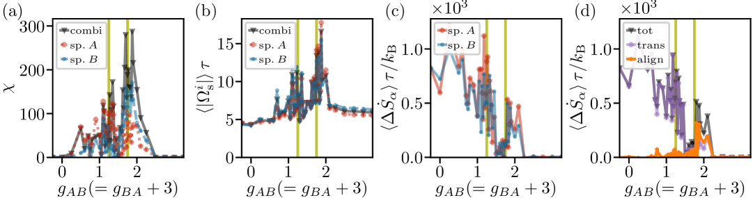
Figure 5: Particle simulation results for a non-reciprocal system with $g_{AB}=g_{BA}+3$. The (a) susceptibility, (b) spontaneous chirality, and (c),(d) particle-averaged entropy production rates are shown as functions of $g_{AB}$. In (c), the entropy production rate is shown separately for both particle species, while in (d) the contributions from translational motion and alignment couplings are plotted separately. Other parameters are as specified in Sec. II.1. The susceptibility and spontaneous chirality are consistent with Ref. Kreienkamp and Klapp (2025).

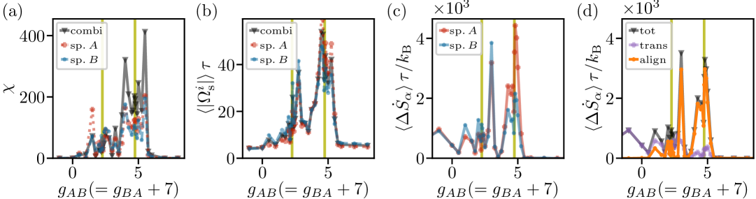
Figure 6: Particle simulation results for a non-reciprocal system with $g_{AB}=g_{BA}+7$. The (a) susceptibility, (b) spontaneous chirality, and (c),(d) particle-averaged entropy production rates are shown as functions of $g_{AB}$. In (c), the entropy production rate is shown separately for both particle species, while in (d) the contributions from translational motion and alignment couplings are plotted separately. Other parameters are as specified in Sec. II.1.

Appendix F Prefactors for polarization perturbations in entropy production rate in the infinite-wavelength limit

In this appendix, we show the analytical prefactors $\gamma$ and $\gamma^{2}$ in the functional (16), which governs the deterministic contribution to the time evolution of polarization perturbations in the infinite-wavelength limit, and of the corresponding entropy production rate (41).

The prefactors in the functional (16) are

$$\begin{split}\bm{\gamma}^{a}_{a}[w_{0}^{a},w_{0}^{b}]&=\begin{pmatrix}\gamma^{a}_{a,\ell}&0\\ 0&\gamma^{a}_{a,t}\end{pmatrix}\\ &=(g^{\prime}-D_{\rm r})\begin{pmatrix}1&0\\ 0&1\end{pmatrix}-\frac{1}{2\,D_{\rm r}}\Big[(g^{\prime}\,\bm{w}_{0}^{a})^{2}\,\begin{pmatrix}3&0\\ 0&1\end{pmatrix}+(g_{ab}^{\prime}\,\bm{w}_{0}^{b})^{2}\begin{pmatrix}1&0\\ 0&1\end{pmatrix}+2\,g^{\prime}\,g_{ab}^{\prime}\,\begin{pmatrix}2&0\\ 0&1\end{pmatrix}\,\bm{w}_{0}^{a}\cdot\bm{w}_{0}^{b}\Big]\end{split}$$ (55)

and

$$\begin{split}\bm{\gamma}^{a}_{b}[w_{0}^{a},w_{0}^{b}]&=\begin{pmatrix}\gamma^{a}_{b,\ell}&0\\ 0&\gamma^{a}_{b,t}\end{pmatrix}\\ &=g_{ab}^{\prime}\begin{pmatrix}1&0\\ 0&1\end{pmatrix}-\frac{1}{D_{\rm r}}\begin{pmatrix}1&0\\ 0&0\end{pmatrix}\Big[g^{\prime}\,g_{ab}^{\prime}\,(\bm{w}_{0}^{a})^{2}+g_{ab}^{\prime 2}\,\bm{w}_{0}^{a}\cdot\bm{w}_{0}^{b}\Big].\end{split}$$ (56)

They are plotted as functions of $g_{AB}=g_{BA}-d$ with $d=5$ in Fig. 7. They do not exhibit special behavior at exceptional points. Nevertheless, they indicate the relevance of different contributions.

Near the exceptional points, certain prefactors of both the flocking [Fig. 7(a)] and antiflocking [Fig. 7(b)] base states – specifically $\gamma^{A}_{B,\ell}$, $\gamma^{B}_{A,t}$ – are positive, while their species-inverted counterparts ($\gamma^{B}_{A,\ell}$, $\gamma^{A}_{B,t}$) are negative but of similar magnitude. This indicates that, in the given parameter regime, longitudinal perturbations in species $B(A)$ enhance (dampen) longitudinal perturbations in $A(B)$. For transversal perturbations, the effect is reversed: transversal perturbations in species $A(B)$ enhance (dampen) transversal perturbations in $B(A)$.

The transversal self-coupling terms, $\gamma^{A}_{A,t}$ and $\gamma^{B}_{B,t}$, have opposite signs and change sign between the flocking to antiflocking base states. This indicates that transversal $A$-perturbations to the flocking state are amplified, whereas transversal $B$-perturbations to the antiflocking state are amplified. In contrast, longitudinal same-species perturbations ($\gamma^{A}_{A,\ell}$ and $\gamma^{B}_{B,\ell}$) are always strongly damped.

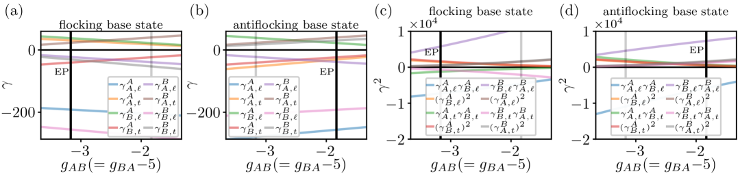
Figure 7: Analytical prefactors in field-theoretical description of polarization perturbations and the corresponding entropy production rate. The prefactors to the functional (16) describing the deterministic contribution to the time evolution of polarization perturbations around the homogeneous (a) flocking and (b) antiflocking base states in the infinite-wavelength limit are shown as functions of $g_{AB}=g_{BA}-5$. In (c) and (d) show the corresponding prefactors of the entropy production rate (41). The vertical black lines indicate the exceptional point associated with the respective base state, while the vertical grey lines mark the exceptional point of the other base state. Note that in (c), the line for $(\gamma_{B,\ell}^{A})^{2}$ (orange) is covered by the line for $(\gamma_{B,t}^{A})^{2}$ (red), and the line for $(\gamma_{A,\ell}^{B})^{2}$ (brown) is covered by the line for $(\gamma_{A,t}^{B})^{2}$ (grey). In (d), the lines for $(\gamma_{B,\ell}^{A})^{2}$ (orange), $\gamma_{A,t}^{A}\,\gamma_{B,t}^{A}$ (green) and $(\gamma_{B,t}^{A})^{2}$ (red) nearly overlap, as do the lines for $(\gamma_{A,\ell}^{B})^{2}$ (brown), $\gamma_{B,t}^{B}\,\gamma_{A,t}^{B}$ (pink) and $(\gamma_{A,t}^{B})^{2}$ (grey).

Figs. 7(c) and (d) display the prefactors of the susceptibilities ($\gamma^{2}$) in the entropy production rate (41) for $g_{AB}=g_{BA}-5$ for flocking [Fig. 7(c)] and antiflocking base states [Fig. 7(d)]. The largest magnitude contributions arise from the terms $\gamma^{A}_{A,\ell}\,\gamma^{A}_{B,\ell}$ and $\gamma^{B}_{B,\ell}\,\gamma^{B}_{A\,\ell}$, pertaining to longitudinal mixed-species susceptibilities along the direction of polarization. However, other contributions, including transversal ones, are also nonzero and remain relevant.

For $d>0$, at the exceptional point associated to the flocking base state, $g_{AB}^{{\rm EP}<}$ (with $g_{AB}^{{\rm EP}<}<g_{AB}^{{\rm EP}>}$), the transversal susceptibility contributions to the entropy production of species $A$ – namely $\gamma^{A}_{A,t}\,\gamma^{A}_{B,t}$ and $(\gamma^{A}_{B,t})^{2}$ – are larger in magnitude than those for species $B$ ($\gamma^{B}_{B,t}\,\gamma^{B}_{A,t}$ and $(\gamma^{B}_{A,t})^{2}$). In contrast, at the exceptional point associated with the antiflocking base state, $g_{AB}^{{\rm EP}>}$, this behavior is reversed: the transversal susceptibility contributions to the entropy production rate of species $B$ are larger than those of species $A$.

This may explain why the entropy production rate of species $A$ peaks at $g_{AB}^{{\rm EP}<}$, while that of species $B$ peaks at $g_{AB}^{{\rm EP}>}$ – both at the particle level (Fig. 4) and in the continuum model (Fig. 8) for $g_{AB}=g_{BA}-5$. Note that this behavior is reversed for $d<0$.

Appendix G Full fluctuating continuum equations

In the main text, we consider only the fluctuating hydrodynamic equations for infinite-wavelength perturbations of the polarization density with respect to homogeneous (anti)flocking base states, as given in Eq. (15). However, one can also write down the fluctuating hydrodynamic equations corresponding to the complete continuum description – including spatial variations in the particle density and polarization density.

To this end, we start from the full deterministic continuum Eqs. (5) and (4) for the particle density and polarization density. Adding noise terms to the (conserved) density and (non-conserved) polarization equations yields the full fluctuating continuum equations, given by

$$\partial_{t}\rho^{a}=-\nabla\cdot\big(\bm{j}^{a}[\rho^{a},\rho^{b},\bm{w}^{a}]+\bm{\xi}^{\rm f}_{a}\big),$$ (57)

with flux

$$\bm{j}^{a}[\rho^{a},\rho^{b},\bm{w}^{a}]=v^{\rm eff}(\rho)\,\bm{w}^{a}-D_{\rm t}\,\nabla\,\rho^{a}$$ (58)

and

$$\partial_{t}\bm{w}^{a}=\bm{\mathcal{F}}^{a}[\rho^{a},\rho^{b},\bm{w}^{a},\bm{w}^{b}]+\bm{\eta}^{\rm f}_{a},$$ (59)

with functional $\bm{\mathcal{F}}^{a}[\rho^{a},\rho^{b},\bm{w}^{a},\bm{w}^{b}]$ as given in Eq. (44), for species $a=A,B$ with $b\neq a$. The noise fields $\bm{\xi}^{\rm f}_{a}(\bm{r},t)$ and $\bm{\eta}^{\rm f}_{a}(\bm{r},t)$ have zero mean. Their variances are

$$\begin{split}\langle\xi_{a,i}^{\rm f}(\bm{r},t)&\,\xi_{b,j}^{\rm f}(\bm{r}^{\prime},t^{\prime})\rangle=2\,D_{\rm h}^{\rho}\,\delta_{ab}\,\delta_{ij}\,\delta(\bm{r}-\bm{r}^{\prime})\,\delta(t-t^{\prime})\end{split}$$ (60)

and

$$\begin{split}\langle\eta_{a,i}^{\rm f}(\bm{r},t)&\,\eta_{b,j}^{\rm f}(\bm{r}^{\prime},t^{\prime})\rangle=2\,D_{\rm h}^{\bm{w}}\,\delta_{ab}\,\delta_{ij}\,\delta(\bm{r}-\bm{r}^{\prime})\,\delta(t-t^{\prime}),\end{split}$$ (61)

respectively. For simplicity, we set $D_{\rm h}^{\rho}=D_{\rm h}^{\bm{w}}=D_{\rm h}$. In our numerical continuum simulations, we set $D_{\rm h}=1\cdot 10^{-5}$.

Appendix H Full entropy production rate in infinite-wavelength limit

In the main text, we analyze the contributions to the entropy production rate arising from perturbations of the polarization field around homogeneous base states in the infinite-wavelength limit. In this appendix, we also consider the infinite-wavelength limit, but provide the analytical calculation of the entropy production rate associated with the full polarization field (not just its perturbations), which involves higher-order correlations. Since the analysis remains restricted to infinite wavelengths, the density field is constant and only the polarization field is taken into account.

The mean-field $k=0$-polarization dynamics for species $a$ is given by Fruchart et al. (2021); Kreienkamp and Klapp (2024a)

$$\partial_{t}\bm{w}^{a}=\bm{\mathcal{F}}^{a}_{k=0}[\bm{w}^{a},\bm{w}^{b}]+\tilde{\bm{\eta}}_{a}$$ (62)

with the deterministic contribution given by the functional

$$\begin{split}&\bm{\mathcal{F}}^{a}_{k=0}[\bm{w}^{a},\bm{w}^{b}]=(g^{\prime}-D_{\rm r}-\frac{(g^{\prime}\,\bm{w}^{a}+g^{\prime}_{ab}\,\bm{w}^{b})^{2}}{2\,D_{\rm r}})\cdot\bm{w}^{a}+g^{\prime}_{ab}\,\bm{w}^{b},\end{split}$$ (63)

where $b\neq a$ and $\bm{w}^{a}=\bm{w}^{a}(\bm{r},t)$, $\tilde{\bm{\eta}}_{a}=\tilde{\bm{\eta}}_{a}(\bm{r},t)$. The alignment strength on the continuum level is given by $g^{\prime}_{ab}=g_{ab}\,R_{\theta}^{2}\,\rho_{0}^{b}/2$. The noise term of strength $D_{\rm h}$ has zero mean and variance

$$\begin{split}\langle\tilde{\eta}_{a,i}(\bm{r},t)&\,\tilde{\eta}_{b,j}(\bm{r}^{\prime},t^{\prime})\rangle=2\,D_{\rm h}\,\delta_{ab}\,\delta_{ij}\,\delta(\bm{r}-\bm{r}^{\prime})\,\delta(t-t^{\prime}).\end{split}$$ (64)

The dynamical action of the forward and backward paths are of the same form as given in Secs. II.4.2 and II.4.3, just with $\bm{\mathcal{F}}^{a}_{k=0,{\rm lin}}[\bm{w}^{\prime a},\bm{w}^{\prime b}]$ replaced by $\bm{\mathcal{F}}^{a}_{k=0}[\bm{w}^{a},\bm{w}^{b}]$. The resulting expression for the informatic entropy production rate is

$$\Delta S^{a}=-\frac{k_{\rm B}}{D_{\rm h}}\iint\big(-(\partial_{t}\bm{w}^{a})\circ\bm{\mathcal{F}}^{a}_{k=0}[\bm{w}^{a},\bm{w}^{b}]\big)\,{\rm d}\bm{r}\,{\rm d}t.$$ (65)

Since the integral in Eq. (65) is a Stratonovich integral, the chain rule applies, and we can rewrite it as

$$\begin{split}\Delta S^{a}=&\frac{k_{\rm B}}{D_{\rm h}}\Bigg(\iint\big(\bm{\mathcal{F}}^{a,{\rm only\ }\bm{w}^{a}}_{k=0}[\bm{w}^{a}]\big)\,{\rm d}\bm{r}\,{\rm d}\bm{w}^{a}+\iint\big((\partial_{t}\bm{w}^{a})\circ\bm{\mathcal{F}}^{a,{\rm also\ }\bm{w}^{b}}_{k=0}[\bm{w}^{a},\bm{w}^{b}]\big)\,{\rm d}\bm{r}\,{\rm d}t\Bigg),\end{split}$$ (66)

where we split $\mathcal{F}^{a}_{k=0}$ into a part that only explicitly depends on $\bm{w}^{a}$,

$$\bm{\mathcal{F}}^{a,{\rm only\,}\bm{w}^{a}}_{k=0}[\bm{w}^{a}]=\big(g^{\prime}-D_{\rm r}-\frac{g^{\prime 2}}{2\,D_{\rm r}}(\bm{w}^{a})^{2}\big)\,\bm{w}^{a},$$ (67)

and a second part that depends (also) on $\bm{w}^{b}$ with $b\neq a$,

$$\begin{split}\bm{\mathcal{F}}^{a,{\rm also\,}\bm{w}^{b}}_{k=0}[\bm{w}^{a},\bm{w}^{b}]=&\ g_{ab}^{\prime}\,\bm{w}^{b}-\frac{g^{\prime 2}_{ab}}{2\,D_{\rm r}}(\bm{w}^{b}\cdot\bm{w}^{b})\,\bm{w}^{a}-\frac{g^{\prime}\,g_{ab}^{\prime}}{D_{\rm r}}\,(\bm{w}^{a}\cdot\bm{w}^{b})\,\bm{w}^{a}.\end{split}$$ (68)

The first part (involving $\bm{\mathcal{F}}^{a,{\rm only\,}\bm{w}^{a}}_{k=0}$) can be integrated directly and yields

$$\begin{split}\Delta S_{1}=&\frac{k_{\rm B}}{D_{\rm h}}\int\bigg(\frac{g^{\prime}-D_{\rm r}}{2}\,(\bm{w}^{a})^{2}-\frac{g^{\prime 2}}{8\,D_{\rm r}}\,(\bm{w}^{a})^{4}\bigg)\,{\rm d}\bm{r}.\end{split}$$ (69)

For the entropy production rate [see Eq. (7)], we take the limit $\tau\rightarrow\infty$. This yields $\Delta S_{1}/\tau\rightarrow 0$, since all moments of $\bm{w}^{a}$ are finite in the steady state.

This leaves us with the second part of the r.h.s. of Eq. (66). Inserting Eq. (62) for $\partial_{t}\bm{w}^{a}$ yields $\Delta S_{2}+\Delta S_{3}$, with

$$\begin{split}\Delta S_{2}=&\frac{k_{\rm B}}{D_{\rm h}}\iint\bm{\mathcal{F}}^{a}_{k=0}\cdot\bm{\mathcal{F}}^{a,{\rm also\,}\bm{w}^{b}}_{k=0}{\rm d}\bm{r}\,{\rm d}t\end{split}$$ (70)

and

$$\begin{split}\Delta S_{3}=&\frac{k_{\rm B}}{D_{\rm h}}\iint\tilde{\bm{\eta}}_{a}\circ\bm{\mathcal{F}}^{a,{\rm also\,}\bm{w}^{b}}_{k=0}\,{\rm d}\bm{r}\,{\rm d}t.\end{split}$$ (71)

While $\Delta S_{2}$ is already independent of the noise and directly yields an entropy production rate upon division by $\tau$ and then taking the limit $\tau\rightarrow\infty$, $\Delta S_{3}$ needs to be calculated explicitly.

We transform the Stratonovich product in $\Delta S_{3}$ into an Itô product, following the transformation rule (37). Since the Itô product vanishes in the equal-time expectation, only the conversion contribution [second contribution on r.h.s. of Eq. (37)] remains to be evaluated.

To calculate the conversion contributions, we consider Fourier space with the Fourier transform defined as

$$\hat{f}(\bm{k})=\int f(\bm{r})\,{\rm e}^{-2\pi i\bm{r}\cdot\bm{k}}\,{\rm d}\bm{r}$$ (72)

and inverse

$$f(\bm{r})=\int\hat{f}(\bm{k})\,{\rm e}^{2\pi i\bm{r}\cdot\bm{k}}\,{\rm d}\bm{r}.$$ (73)

In Fourier space the noise correlation $\langle\tilde{\eta}_{\alpha}(\bm{r},t)\,\tilde{\eta}_{\beta}(\bm{r}^{\prime},t^{\prime})\rangle$, given in Eq. (64), transforms into

$$\begin{split}\frac{\langle\hat{\tilde{\eta}}_{\alpha}(\bm{k},t)\,\hat{\tilde{\eta}}_{\beta}(\bm{k}^{\prime},t^{\prime})\rangle}{2\,D_{\rm h}\,\delta_{\alpha\beta}\,\delta(t-t^{\prime})}&=\iint\delta(\bm{r}-\bm{r}^{\prime})\,{\rm e}^{-2\pi i(\bm{r}\cdot\bm{k}+\bm{r}^{\prime}\cdot\bm{k}^{\prime})}\,{\rm d}{\bm{r}}\,{\rm d}\bm{r}^{\prime}\\ &=\iint\,{\rm e}^{-2\pi i\bm{r}\cdot(\bm{k}+\bm{k}^{\prime})}\,{\rm d}{\bm{r}}\\ &=\delta(\bm{k}+\bm{k}^{\prime}).\end{split}$$ (74)

We now go through the individual terms in $\Delta S_{3}$ step-by-step. The first term is zero, i.e.,

$$\begin{split}\Delta S_{3.1}=&\frac{k_{\rm B}}{D_{\rm h}}\,g_{ab}^{\prime}\iint\bm{w}^{b}\circ\tilde{\bm{\eta}}_{a}\,{\rm d}\bm{r}\,{\rm d}t=0,\end{split}$$ (75)

because, here, the Stratonovich product coincides with the corresponding Itô product. For the second term,

$$\begin{split}\Delta S_{3.2}=&-\frac{k_{\rm B}}{D_{\rm h}}\,\frac{g_{ab}^{\prime 2}}{2\,D_{\rm r}}\iint(\bm{w}^{b}\cdot\bm{w}^{b})\,\bm{w}^{a}\circ\tilde{\bm{\eta}}_{a}\,{\rm d}\bm{r}\,{\rm d}t,\end{split}$$ (76)

we assume that we can replace temporal averages by averages over noise realizations. For the entropy production rate, this implies

$$\begin{split}\Delta\dot{S}_{3.2}&=-\frac{k_{\rm B}}{D_{\rm h}}\,\frac{g_{ab}^{\prime 2}}{2\,D_{\rm r}}\left\langle\int(\bm{w}^{b}\cdot\bm{w}^{b})\,\bm{w}^{a}\circ\tilde{\bm{\eta}}_{a}\,{\rm d}\bm{r}\right\rangle\\ &=-k_{\rm B}\,\frac{g_{ab}^{\prime 2}}{D_{\rm r}}\,\delta(\bm{0})\left\langle\int(\bm{w}^{b}\cdot\bm{w}^{b})\,{\rm d}\bm{r}\right\rangle\end{split}$$ (77)

Note that the two dimensions lead to the factor of $2$. The $\delta(\bm{0})$ appears due to the equal-position product [i.e., $\bm{r}=\bm{r}^{\prime}$ in Eq. (37)]. The third term is

$$\begin{split}\Delta S_{3.3}&=-\frac{k_{\rm B}}{D_{\rm h}}\,\frac{g^{\prime}\,g_{ab}^{\prime}}{D_{\rm r}}\left\langle\int(\bm{w}^{a}\cdot\bm{w}^{b})\,\bm{w}^{a}\circ\tilde{\bm{\eta}}_{a}\,{\rm d}\bm{r}\right\rangle\\ &=-k_{\rm B}\,\frac{g^{\prime}\,g_{ab}^{\prime}}{D_{\rm r}}\,\delta(\bm{0})\,\left\langle\int 3\,(\bm{w}^{a}\cdot\bm{w}^{b})\,{\rm d}\bm{r}\right\rangle\end{split}$$ (78)

This entropy production contribution depends on the system size due to the $\delta(\bm{0})=\int{\rm e}^{-2\pi i\bm{r}\cdot\bm{k}}|_{\bm{k}=\bm{0}}\,{\rm d}\bm{r}=L^{2}$.

The resulting entropy production rate reads

$$\begin{split}\Delta\dot{S}=\,&k_{\rm B}\,\int\Bigg(\frac{1}{D_{\rm h}}\left\langle\bm{\mathcal{F}}^{a}_{k=0}\cdot\bm{\mathcal{F}}^{a,{\rm also\,}\bm{w}^{b}}_{k=0}\right\rangle-\frac{\delta(\bm{0})}{D_{\rm r}}\,\Big\langle g_{ab}^{\prime 2}\,(\bm{w}^{b})^{2}+3\,g^{\prime}\,g^{\prime}_{ab}\,\bm{w}^{a}\cdot\bm{w}^{b}\Big\rangle\Bigg)\,{\rm d}\bm{r}.\end{split}$$ (79)

This result can, in principle, be used to investigate analytically the scaling of the entropy production with the noise strength $D_{\rm h}$, as done, e.g., for phase separating Nardini et al. (2017), flocking Borthne et al. (2020); Dadhichi et al. (2018), and non-reciprocal scalar systems Suchanek et al. (2023c), to quantify the nature of time-reversal symmetry breaking Fodor et al. (2022). To this end, one would need to define proper ground state trajectories to obtain meaningful scalings regarding the transition to, e.g., chiral states.

Appendix I Full entropy production rate at arbitrary wavelengths from numerical continuum simulations

The entropy production rate associated with infinite-wavelength polarization fluctuations considered in the main text allows for analytical insights. However, to obtain a more complete picture, one can also consider the entropy production rate derived from the full continuum description, as given in Appendix G, which involves both the particle density and polarization density.

The dynamical action of the trajectory $\vec{\bm{\varphi}}=\{(\rho^{A}(t),\rho^{B}(t),\bm{w}^{A}(t),\bm{w}^{B}(t))|t\in[t_{0},\tau]\}$ contains contributions from both the densities and polarization densities of both species, i.e.,

$$\mathcal{A}[\vec{\bm{\varphi}}]=\mathcal{A}_{\rho^{A}}+\mathcal{A}_{\rho^{B}}+\mathcal{A}_{\bm{w}^{A}}+\mathcal{A}_{\bm{w}^{B}}.$$ (80)

The density contributions are given by Nardini et al. (2017)

$$\begin{split}\mathcal{A}_{\rho^{a}}=&\frac{1}{4\,D_{\rm h}}\iint\Big(\nabla^{-1}(\partial_{t}\rho^{a}+\nabla\cdot\bm{j}^{a}[\rho^{a},\rho^{b},\bm{w}^{a}])\Big)^{2}\,{\rm d}\bm{r}\,{\rm d}t+\mathcal{A}_{\rho^{a}}^{\rm conv},\end{split}$$ (81)

where $\nabla^{-1}X=\nabla\,\nabla^{-2}X$ for a scalar $X$, and $\nabla^{-2}$ is the functional inverse to the Laplacian Nardini et al. (2017) . The polarization contributions are, similarly to what is discussed in the main text,

$$\begin{split}\mathcal{A}_{\bm{w}^{a}}=&\frac{1}{4\,D_{\rm h}}\iint\Big(\partial_{t}\bm{w}^{a}-\bm{\mathcal{F}}^{a}[\rho^{a},\rho^{b},\bm{w}^{a},\bm{w}^{b}]\Big)^{2}\,{\rm d}\bm{r}\,{\rm d}t+\mathcal{A}_{\bm{w}^{a}}^{\rm conv}.\end{split}$$ (82)

For Stratonovich discretization, the terms that depend explicitly on the choice of time discretization with respect to noise, are

$$\mathcal{A}_{\rho^{a}}^{\rm conv}=-\dfrac{1}{2}\iint\frac{\delta\nabla\cdot\bm{j}_{a}[\rho^{a},\rho^{b},\bm{w}^{a}]}{\delta\rho^{a}}\,{\rm d}\bm{r}\,{\rm d}t$$ (83)

and

$$\mathcal{A}_{\bm{w}^{a}}^{\rm conv}=\dfrac{1}{2}\iint\frac{\delta\bm{\mathcal{F}}^{a}[\rho^{a},\rho^{b},\bm{w}^{a},\bm{w}^{b}]}{\delta\bm{w}^{a}}\,{\rm d}\bm{r}\,{\rm d}t.$$ (84)

To calculate the entropy production rate as the ratio between forward and backward path probabilities, we must consider the time-reversed density, which is even under time-reversal, i.e.,

$$\rho^{a\dagger}(\bm{r},t)=\rho^{a}(\bm{r},\tau+t_{0}-t)$$ (85)

and the time-reversed polarization density, which we consider odd under time-reversal, i.e.,

$$\bm{w}^{a\dagger}(\bm{r},t)=-\bm{w}^{a}(\bm{r},\tau+t_{0}-t).$$ (86)

The functional $\bm{\mathcal{F}}^{a}[\rho^{a},\rho^{b},\bm{w}^{a},\bm{w}^{b}]$, which governs the time evolution of $\bm{w}^{a}$, can be split into time-symmetric and time-anti-symmetric contributions, which satisfy

$$\bm{\mathcal{F}}^{a}_{\rm sym}[\rho^{a\dagger},\rho^{b\dagger},\bm{w}^{a\dagger},\bm{w}^{b\dagger}]=\bm{\mathcal{F}}^{a}_{\rm sym}[\rho^{a},\rho^{b},\bm{w}^{a},\bm{w}^{b}]$$ (87)

and

$$\bm{\mathcal{F}}^{a}_{\rm asym}[\rho^{a\dagger},\rho^{b\dagger},\bm{w}^{a\dagger},\bm{w}^{b\dagger}]=-\bm{\mathcal{F}}^{a}_{\rm asym}[\rho^{a},\rho^{b},\bm{w}^{a},\bm{w}^{b}].$$ (88)

They are given by

$$\begin{split}\bm{\mathcal{F}}^{a}_{\rm sym}[\rho^{a},\rho^{b},\bm{w}^{a},\bm{w}^{b}]=&-\frac{1}{2}\,\nabla\,\big(v^{\rm eff}(\rho)\,\rho^{a}\big)+\sum_{b}\frac{g^{\prime}_{ab}}{8\,D_{\rm r}}\Big[\bm{w}^{b}\cdot\nabla\big(v^{\rm eff}(\rho)\,\bm{w}^{a}\big)+\bm{w}^{b*}\cdot\nabla\big(v^{\rm eff}(\rho)\,\bm{w}^{a*}\big)\\ &-2\,\Big\{v^{\rm eff}(\rho)\,\bm{w}^{a}\cdot\nabla\bm{w}^{b}+\bm{w}^{b}\,\nabla\cdot\big(v^{\rm eff}(\rho)\,\bm{w}^{a}\big)-v^{\rm eff}(\rho)\,\bm{w}^{a*}\cdot\nabla\bm{w}^{b*}-\bm{w}^{b*}\,\nabla\cdot\big(v^{\rm eff}(\rho)\,\bm{w}^{a*}\big)\Big\}\Big],\end{split}$$ (89)

and

$$\begin{split}\bm{\mathcal{F}}^{a}_{\rm asym}[\rho^{a},\rho^{b},\bm{w}^{a},\bm{w}^{b}]=&-D_{\rm r}\,\bm{w}^{a}+\sum_{b}g^{\prime}_{ab}\,\rho^{a}\,\bm{w}^{b}+D_{\rm t}\,\nabla^{2}\,\bm{w}^{a}+\frac{v^{\rm eff}(\rho)}{16\,D_{\rm r}}\,\nabla^{2}\,\Big(v^{\rm eff}(\rho)\,\bm{w}^{a}\Big)\\ &-\sum_{b,c}\frac{g^{\prime}_{ab}\,g^{\prime}_{ac}}{2\,D_{\rm r}}\,\bm{w}^{a}\,(\bm{w}^{b}\cdot\bm{w}^{c})-\frac{z}{16\,D_{\rm r}}\,\nabla\rho\cdot\big[\nabla\big(v^{\rm eff}(\rho)\,\bm{w}^{a}\big)-\nabla^{*}\big(v^{\rm eff}(\rho)\,\bm{w}^{a*}\big)\big].\end{split}$$ (90)

The action of the time-reversed trajectory is given by

$$\mathcal{A}[\vec{\bm{\varphi}}^{\prime\dagger}]=\overleftarrow{\mathcal{A}}_{\rho^{A}}+\overleftarrow{\mathcal{A}}_{\rho^{B}}+\overleftarrow{\mathcal{A}}_{\bm{w}^{A}}+\overleftarrow{\mathcal{A}}_{\bm{w}^{B}}$$ (91)

with

$$\begin{split}\overleftarrow{\mathcal{A}}_{\rho^{a}}=&\iint\Big(\nabla^{-1}(\partial_{t}\rho^{a\dagger}+\nabla\cdot\bm{j}^{a}[\rho^{a\dagger},\rho^{b\dagger},\bm{w}^{a\dagger}])\Big)^{2}\,{\rm d}\bm{r}\,{\rm d}t+\overleftarrow{\mathcal{A}}_{\rho^{a}}^{\rm conv},\end{split}$$ (92)

where

$$\overleftarrow{\mathcal{A}}_{\rho^{a}}^{\rm conv}=-\dfrac{1}{2}\iint\frac{\delta\nabla\cdot\bm{j}_{a}[\rho^{a\dagger},\rho^{b\dagger},\bm{w}^{a\dagger}]}{\delta\rho^{a\dagger}}\,{\rm d}\bm{r}\,{\rm d}t,$$ (93)

and

$$\begin{split}\overleftarrow{\mathcal{A}}_{\bm{w}^{a}}=&\frac{1}{4\,D_{\rm h}}\iint\big(\partial_{t}\bm{w}^{a\dagger}-\bm{\mathcal{F}}^{a}[\rho^{a\dagger},\rho^{b\dagger},\bm{w}^{a\dagger},\bm{w}^{b\dagger}]\big)^{2}\,{\rm d}\bm{r}\,{\rm d}t+\overleftarrow{\mathcal{A}}_{\bm{w}^{a}}^{\rm conv},\end{split}$$ (94)

where

$$\overleftarrow{\mathcal{A}}_{\bm{w}^{a}}^{\rm conv}=\dfrac{1}{2}\iint\frac{\delta\bm{\mathcal{F}}^{a}[\rho^{a\dagger},\rho^{b\dagger},\bm{w}^{a\dagger},\bm{w}^{b\dagger}]}{\delta\bm{w}^{a\dagger}}\,{\rm d}\bm{r}\,{\rm d}t.$$ (95)

Hence, the entropy production related to the density and polarization dynamics of species $a$ are

$$\begin{split}\Delta S^{a}_{\rho^{a}}=&k_{\rm B}\,\left(\overleftarrow{\mathcal{A}}_{\rho^{a}}-\mathcal{A}_{\rho^{a}}\right)\\ =&-\frac{k_{\rm B}}{D_{\rm h}}\iint\Big(\nabla^{-2}\Big(-(\partial_{t}\rho^{a})\circ(D_{\rm t}\,\nabla^{2}\rho^{a})\Big)-(v^{\rm eff}(\rho)\,\bm{w}^{a}))\cdot(D_{\rm t}\,\nabla\rho^{a})\Big)\,{\rm d}\bm{r}\,{\rm d}t\\ &+\iint\frac{\delta\nabla\cdot(v^{\rm eff}(\rho)\,\bm{w}^{a})}{\delta\rho^{a}}\,{\rm d}\bm{r}\,{\rm d}t\end{split}$$ (96)

and

$$\begin{split}\Delta S^{a}_{\bm{w}^{a}}&=k_{\rm B}\,\left(\overleftarrow{\mathcal{A}}_{\bm{w}^{a}}-\mathcal{A}_{\bm{w}^{a}}\right)\\ &=\frac{k_{\rm B}}{D_{\rm h}}\iint\Big((\partial_{t}\bm{w}^{a})\circ\bm{\mathcal{F}}^{a}_{\rm asym}-\bm{\mathcal{F}}^{a}_{\rm asym}\cdot\bm{\mathcal{F}}^{a}_{\rm sym}\Big)\,{\rm d}\bm{r}\,{\rm d}t+\iint\frac{\delta\bm{\mathcal{F}}_{\rm sym}^{a}}{\delta\bm{w}^{a}}{\rm d}\bm{r}\,{\rm d}t,\end{split}$$ (97)

respectively. The total entropy production rate, $\Delta\dot{S}^{a}=\Delta\dot{S}^{a}_{\rho^{a}}+\Delta\dot{S}^{a}_{\bm{w}^{a}}$, is then calculated as the time-averaged mean, defined in Eq. (7).

Following the line of calculations shown in Appendix H for the (simpler) infinite-wavelength limit, where density dynamics and gradient terms are neglected, one can, in principle, obtain an analytical expression for the full entropy production rate involving spatially varying density and polarization fields. However, as already indicated by the final expression in Appendix H, given in Eq. (79), the resulting formula is lengthy, depends on the system size, and cannot be easily interpreted to yield meaningful insights.

Therefore, we turn to numerical continuum simulations (for details on the continuum simulation methods, see Appendix C.2). Fig. 8 shows the entropy production rate obtained from continuum simulations of the full fluctuating hydrodynamic Eqs. (57)-(59) for the case $g_{AB}=g_{BA}-d$ with $d=5$ and $d=-7$. Generally, these results are not expected to quantitatively match the particle-level results presented in the main text. One reason is the choice of the noise strength $D_{\rm h}$, which lacks a clear microscopic counterpart and is set, ad hoc, equal for both particle density and polarization density. Nevertheless, the general dependence of the entropy production rate on the coupling strength shows qualitative similarities to the one obtained from particle simulations shown in Fig. 4.

In particular, for $d=5$ [Fig. 8(a)], the total entropy production rate in the continuum system (as the sum of $A$- and $B$-species contributions) also exhibits peaks at the exceptional points. As suggested by the prefactors of the susceptibilities in the analytical expression (41) for the entropy production rate (see Appendix F), the $A$-species peak occurs near the exceptional point $g_{AB}^{{\rm EP}<}$ (with $g_{AB}^{{\rm EP}<}<g_{AB}^{{\rm EP}>}$), while the $B$-species peak appears near $g_{AB}^{{\rm EP}>}$. This behavior is consistent with the particle simulation results (in Fig. 4).

An apparent difference between the continuum and particle results concerns the translational and orientational contributions to the entropy production rate [Fig. 8(b)]. While at the particle level, the translational dynamics significantly contribute to the entropy production rate in the antiflocking regime, at the continuum level (with equal noise strengths for particle density and polarization density), the entropy production is almost exclusively governed by the polarization density dynamics within all regimes. However, these two levels of description are not directly comparable: on the particle level, the orientational contributions [Eq. (13)] account solely for particle orientations, whereas the polarization density field combines the director (unit vector) and the particle density, thus blending different aspects [in Eq. (97)].

To demonstrate that this behavior is consistent for different $d$, we show the entropy production rate of the continuum system for $g_{AB}=g_{BA}+7$ in Fig. 8(c) and (d). This non-reciprocal system also exhibits peaks near the exceptional points, with the small shift of the peak at $g_{AB}^{{\rm EP}<}$ observed at both the particle and continuum levels. Notably, as for the particle system (Fig. 6), the peaks of $A$- and $B$-species entropy production are reversed compared to the case of $g_{AB}=g_{BA}-5$.

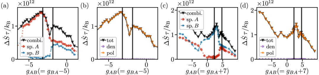
Figure 8: Continuum-level entropy production rate of non-reciprocal systems obtained from continuum simulations with (a),(b) $g_{AB}=g_{BA}-5$ and (c),(d) $g_{AB}=g_{BA}+7$. In (a),(c), the contributions from individual species are shown in red and blue, while the black data points indicates their sum. In (b),(d), the contributions from the polarization and density are shown in orange and purple, respectively, while their sum is shown in black. Black vertical lines indicate parameters associated with exceptional points. The data shows simulation results between $330\,\tau$ and $350\,\tau$ after initialization.

An interesting question is how the noise amplitude, or different noise strengths in the density and polarization dynamics, affect the entropy production at the field level. We leave this question for further investigation.

References

- Seifert (2012) Udo Seifert, “Stochastic thermodynamics, fluctuation theorems and molecular machines,” Rep. Prog. Phys. 75, 126001 (2012).
- Peliti and Pigolotti (2021) Luca Peliti and Simone Pigolotti, Stochastic thermodynamics: an introduction (Princeton University Press, 2021).
- Fodor et al. (2022) Étienne Fodor, Robert L Jack, and Michael E Cates, “Irreversibility and biased ensembles in active matter: Insights from stochastic thermodynamics,” Annu. Rev. Condens. Matter Phys. 13, 215–238 (2022).
- O’Byrne et al. (2022) Jérémy O’Byrne, Yariv Kafri, Julien Tailleur, and Frédéric van Wijland, “Time irreversibility in active matter, from micro to macro,” Nature Reviews Physics 4, 167–183 (2022).
- Dabelow et al. (2019) Lennart Dabelow, Stefano Bo, and Ralf Eichhorn, “Irreversibility in active matter systems: Fluctuation theorem and mutual information,” Phys. Rev. X 9, 021009 (2019).
- Pietzonka et al. (2019) Patrick Pietzonka, Étienne Fodor, Christoph Lohrmann, Michael E Cates, and Udo Seifert, “Autonomous engines driven by active matter: Energetics and design principles,” Phys. Rev. X 9, 041032 (2019).
- Bebon et al. (2025) Robin Bebon, Joshua F Robinson, and Thomas Speck, “Thermodynamics of active matter: Tracking dissipation across scales,” Phys. Rev. X 15, 021050 (2025).
- Loos and Klapp (2020) Sarah A M Loos and Sabine H L Klapp, “Irreversibility, heat and information flows induced by non-reciprocal interactions,” New J. Phys. 22, 123051 (2020).
- Loos et al. (2021) Sarah A M Loos, Simon Hermann, and Sabine H L Klapp, “Medium entropy reduction and instability in stochastic systems with distributed delay,” Entropy 23, 696 (2021).
- Saha et al. (2020) Suropriya Saha, Jaime Agudo-Canalejo, and Ramin Golestanian, “Scalar active mixtures: The nonreciprocal Cahn-Hilliard model,” Phys. Rev. X 10, 041009 (2020).
- Ivlev et al. (2015) Alexei V Ivlev, Jörg Bartnick, Marco Heinen, C-R Du, V Nosenko, and Hartmut Löwen, “Statistical mechanics where Newton’s third law is broken,” Phys. Rev. X 5, 011035 (2015).
- Scheibner et al. (2020) Colin Scheibner, Anton Souslov, Debarghya Banerjee, Piotr Surówka, William TM Irvine, and Vincenzo Vitelli, “Odd elasticity,” Nat. Phys. 16, 475–480 (2020).
- Bowick et al. (2022) Mark J. Bowick, Nikta Fakhri, M. Cristina Marchetti, and Sriram Ramaswamy, “Symmetry, thermodynamics, and topology in active matter,” Phys. Rev. X 12, 010501 (2022).
- Lotka (1920) Alfred J Lotka, “Analytical note on certain rhythmic relations in organic systems,” Proc. Natl. Acad. Sci. U.S.A. 6, 410–415 (1920).
- Volterra (1926) Vito Volterra, “Fluctuations in the abundance of a species considered mathematically,” Nature 118, 558–560 (1926).
- Xiong et al. (2020) Liyang Xiong, Yuansheng Cao, Robert Cooper, Wouter-Jan Rappel, Jeff Hasty, and Lev Tsimring, “Flower-like patterns in multi-species bacterial colonies,” eLife 9, e48885 (2020).
- Pruessner and Garcia-Millan (2022) Gunnar Pruessner and Rosalba Garcia-Millan, “Field theories of active particle systems and their entropy production,” arXiv preprint arXiv:2211.11906 (2022).
- Brossollet and Biroli (2025) Antonin Brossollet and Giulio Biroli, “Entropy production from density field theories for interacting particles systems,” arXiv preprint arXiv:2507.15131 (2025).
- Nardini et al. (2017) Cesare Nardini, Étienne Fodor, Elsen Tjhung, Frédéric Van Wijland, Julien Tailleur, and Michael E Cates, “Entropy production in field theories without time-reversal symmetry: quantifying the non-equilibrium character of active matter,” Phys. Rev. X 7, 021007 (2017).
- Borthne et al. (2020) Øyvind L Borthne, Étienne Fodor, and Michael E Cates, “Time-reversal symmetry violations and entropy production in field theories of polar active matter,” New J. Phys. 22, 123012 (2020).
- Ferretti et al. (2022) Federica Ferretti, Simon Grosse-Holz, Caroline Holmes, Jordan L Shivers, Irene Giardina, Thierry Mora, and Aleksandra M Walczak, “Signatures of irreversibility in microscopic models of flocking,” Phys. Rev. E 106, 034608 (2022).
- Proesmans et al. (2025) Karel Proesmans, Gianmaria Falasco, Atul Tanaji Mohite, Massimiliano Esposito, and Étienne Fodor, “Quantifying dissipation in flocking dynamics: When tracking internal states matter,” arXiv preprint arXiv:2505.13113 (2025).
- Martynec et al. (2020) Thomas Martynec, Sabine HL Klapp, and Sarah AM Loos, “Entropy production at criticality in a nonequilibrium potts model,” New Journal of Physics 22, 093069 (2020).
- Herpich et al. (2018) Tim Herpich, Juzar Thingna, and Massimiliano Esposito, “Collective power: minimal model for thermodynamics of nonequilibrium phase transitions,” Phys. Rev. X 8, 031056 (2018).
- Meibohm and Esposito (2024) Jan Meibohm and Massimiliano Esposito, “Minimum-dissipation principle for synchronized stochastic oscillators far from equilibrium,” Phys. Rev. E 110, L042102 (2024).
- Seara et al. (2021) Daniel S Seara, Benjamin B Machta, and Michael P Murrell, “Irreversibility in dynamical phases and transitions,” Nature communications 12, 392 (2021).
- Dinelli et al. (2023) Alberto Dinelli, Jérémy O’Byrne, Agnese Curatolo, Yongfeng Zhao, Peter Sollich, and Julien Tailleur, “Non-reciprocity across scales in active mixtures,” Nat. Commun. 14, 7035 (2023).
- Alston et al. (2023) Henry Alston, Luca Cocconi, and Thibault Bertrand, “Irreversibility across a nonreciprocal pt-symmetry-breaking phase transition,” Phys. Rev. Lett. 131, 258301 (2023).
- Suchanek et al. (2023a) Thomas Suchanek, Klaus Kroy, and Sarah A M Loos, “Irreversible mesoscale fluctuations herald the emergence of dynamical phases,” Phys. Rev. Lett. 131, 258302 (2023a).
- Suchanek et al. (2023b) Thomas Suchanek, Klaus Kroy, and Sarah A M Loos, “Entropy production in the nonreciprocal Cahn-Hilliard model,” Phys. Rev. E 108, 064610 (2023b).
- Loos et al. (2023) Sarah A M Loos, Sabine H L Klapp, and Thomas Martynec, “Long-range order and directional defect propagation in the nonreciprocal XY model with vision cone interactions,” Phys. Rev. Lett. 130, 198301 (2023).
- You et al. (2020) Zhihong You, Aparna Baskaran, and M. Cristina Marchetti, “Nonreciprocity as a generic route to traveling states,” Proc. Natl. Acad. Sci. U.S.A. 117, 19767 (2020).
- Fruchart et al. (2021) Michel Fruchart, Ryo Hanai, Peter B Littlewood, and Vincenzo Vitelli, “Non-reciprocal phase transitions,” Nature 592, 363 (2021).
- Kreienkamp and Klapp (2025) Kim L Kreienkamp and Sabine H L Klapp, “Synchronization and exceptional points in nonreciprocal active polar mixtures,” Commun. Phys. 8, 307 (2025).
- Kreienkamp and Klapp (2024a) Kim L Kreienkamp and Sabine H L Klapp, “Nonreciprocal alignment induces asymmetric clustering in active mixtures,” Phys. Rev. Lett. 133, 258303 (2024a).
- Kreienkamp and Klapp (2024b) Kim L Kreienkamp and Sabine H L Klapp, “Dynamical structures in phase-separating nonreciprocal polar active mixtures,” Phys. Rev. E 110, 064135 (2024b).
- Kreienkamp and Klapp (2022) Kim L Kreienkamp and Sabine H L Klapp, “Clustering and flocking of repulsive chiral active particles with non-reciprocal couplings,” New J. Phys. 24, 123009 (2022).
- Cates and Tailleur (2015) Michael E Cates and Julien Tailleur, “Motility-induced phase separation,” Annu. Rev. Condens. Matter Phys. 6, 219–244 (2015).
- Bialké et al. (2013) Julian Bialké, Hartmut Löwen, and Thomas Speck, “Microscopic theory for the phase separation of self-propelled repulsive disks,” EPL 103, 30008 (2013).
- Marchetti et al. (2013) M Cristina Marchetti, Jean-François Joanny, Sriram Ramaswamy, Tanniemola B Liverpool, Jacques Prost, Madan Rao, and R Aditi Simha, “Hydrodynamics of soft active matter,” Rev. Mod. Phys. 85, 1143 (2013).
- Vicsek et al. (1995) Tamás Vicsek, András Czirók, Eshel Ben-Jacob, Inon Cohen, and Ofer Shochet, “Novel type of phase transition in a system of self-driven particles,” Phys. Rev. Lett. 75, 1226 (1995).
- Grégoire and Chaté (2004) Guillaume Grégoire and Hugues Chaté, “Onset of collective and cohesive motion,” Phys. Rev. Lett. 92, 025702 (2004).
- Weeks et al. (1971) John D Weeks, David Chandler, and Hans C Andersen, “Role of repulsive forces in determining the equilibrium structure of simple liquids,” J. Chem. Phys. 54, 5237 (1971).
- El-Ganainy et al. (2018) Ramy El-Ganainy, Konstantinos G Makris, Mercedeh Khajavikhan, Ziad H Musslimani, Stefan Rotter, and Demetrios N Christodoulides, “Non-Hermitian physics and PT symmetry,” Nat. Phys. 14, 11–19 (2018).
- Suchanek et al. (2023c) Thomas Suchanek, Klaus Kroy, and Sarah A M Loos, “Time-reversal and parity-time symmetry breaking in non-Hermitian field theories,” Phys. Rev. E 108, 064123 (2023c).
- Seifert (2005) Udo Seifert, “Entropy production along a stochastic trajectory and an integral fluctuation theorem,” Phys. Rev. Lett. 95, 040602 (2005).
- Seifert (2008) Udo Seifert, “Stochastic thermodynamics: principles and perspectives,” Eur. Phys. J. B 64, 423–431 (2008).
- Spinney and Ford (2012) Richard E Spinney and Ian J Ford, “Entropy production in full phase space for continuous stochastic dynamics,” Phys. Rev. E 85, 051113 (2012).
- Crosato et al. (2019) Emanuele Crosato, Mikhail Prokopenko, and Richard E Spinney, “Irreversibility and emergent structure in active matter,” Phys. Rev. E 100, 042613 (2019).
- Shankar and Marchetti (2018) Suraj Shankar and M Cristina Marchetti, “Hidden entropy production and work fluctuations in an ideal active gas,” Phys. Rev. E 98, 020604 (2018).
- Note (1) Note that the sum of the odd and even entropy production is a constant, such that peaks in the entropy production rate with odd interpretation also occur for even interpretation Pietzonka and Seifert (2017); Dadhichi et al. (2018).
- Mohite and Rieger (2025) Atul Tanaji Mohite and Heiko Rieger, “Stochastic thermodynamics of non-reciprocally interacting particles and fields,” arXiv preprint arXiv:2504.10515 (2025).
- Yu and Tu (2022) Qiwei Yu and Yuhai Tu, “Energy cost for flocking of active spins: the cusped dissipation maximum at the flocking transition,” Phys. Rev. Lett. 129, 278001 (2022).
- Note (2) Note that, in one-species systems, the entropy production rate associated with the alignment couplings exhibits a peak at the transition from disordered to flocking motion Ferretti et al. (2022); Yu and Tu (2022). Here, we do not study the conventional ordered-disorder transition. Instead, we consider a binary mixture transitioning from antiflocking to flocking as is varied.
- Toner et al. (2005) John Toner, Yuhai Tu, and Sriram Ramaswamy, “Hydrodynamics and phases of flocks,” Ann. Phys. 318, 170 (2005).
- Dadhichi et al. (2018) Lokrshi Prawar Dadhichi, Ananyo Maitra, and Sriram Ramaswamy, “Origins and diagnostics of the nonequilibrium character of active systems,” J. Stat. Mech.: Theory Exp. 2018, 123201 (2018).
- Onsager and Machlup (1953) Lars Onsager and Stefan Machlup, “Fluctuations and irreversible processes,” Phys. Rev. 91, 1505 (1953).
- Cates et al. (2022) Michael E Cates, Étienne Fodor, Tomer Markovich, Cesare Nardini, and Elsen Tjhung, “Stochastic hydrodynamics of complex fluids: Discretisation and entropy production,” Entropy 24, 254 (2022).
- Cugliandolo and Lecomte (2017) Leticia F Cugliandolo and Vivien Lecomte, “Rules of calculus in the path integral representation of white noise Langevin equations: the Onsager–Machlup approach,” J. Phys. A-Math. Theor. 50, 345001 (2017).
- Note (3) Note that and cancel when the functional is fully anti-symmetric in time (as in this case). This is not generally the case.
- Gardiner (1985) Crispin W Gardiner, Handbook of stochastic methods, Vol. 3 (Springer Berlin, 1985).
- Note (4) In Itô calculus, the delta-correlated noise only affects at later time steps, making and uncorrelated at equal times.
-
Note (5)
This conversion is commonly presented for particles and
unit-variance noise, e.g., Gardiner (1985); Cates et al. (2022):
for a Langevin equation
for , where , and , , one has Cates et al. (2022)(98)
where is a function of . In our field-theoretical case, the noise has no unit-variance but ‘includes’ the . Therefore, the additional prefactor needs to be taken into account.(99) - Soriani et al. (2025) Artur Soriani, Elsen Tjhung, Étienne Fodor, and Tomer Markovich, “Control of active field theories at minimal dissipation,” arXiv preprint arXiv:2504.19285 (2025).
- Garcia-Millan et al. (2024) Rosalba Garcia-Millan, Janik Schüttler, Michael E Cates, and Sarah A M Loos, “Optimal closed-loop control of active particles and a minimal information engine,” arXiv preprint arXiv:2407.18542 (2024).
- Loos et al. (2024) Sarah AM Loos, Samuel Monter, Felix Ginot, and Clemens Bechinger, “Universal symmetry of optimal control at the microscale,” Phys. Rev. X 14, 021032 (2024).
- Li et al. (2024) Junang Li, Chih-Wei Joshua Liu, Michal Szurek, and Nikta Fakhri, “Measuring irreversibility from learned representations of biological patterns,” Phys. Rev. X Life 2, 033013 (2024).
- Tan et al. (2021) Tzer Han Tan, Garrett A Watson, Yu-Chen Chao, Junang Li, Todd R Gingrich, Jordan M Horowitz, and Nikta Fakhri, “Scale-dependent irreversibility in living matter,” arXiv preprint arXiv:2107.05701 (2021).
- Seifert (2019) Udo Seifert, “From stochastic thermodynamics to thermodynamic inference,” Annu. Rev. Condens. Matter Phys. 10, 171–192 (2019).
- Liu et al. (2025) Shuoguang Liu, Ryo Hanai, and Peter B Littlewood, “Universal scaling in one-dimensional non-reciprocal matter,” arXiv preprint arXiv:2503.14384 (2025).
- Risken and Risken (1996) Hannes Risken and Hannes Risken, Fokker-Planck equation (Springer, 1996).
- Note (6) To evaluate a Stratonovich product of form with stochastic variable , one computes , where is evaluated at the mid points , and Risken and Risken (1996).
- Canuto et al. (2007) Claudio Canuto, M Yousuff Hussaini, Alfio Quarteroni, and Thomas A Zang, Spectral methods: fundamentals in single domains (Springer Science & Business Media, 2007).
- Martín-Gómez et al. (2018) Aitor Martín-Gómez, Demian Levis, Albert Díaz-Guilera, and Ignacio Pagonabarraga, “Collective motion of active Brownian particles with polar alignment,” Soft Matter 14, 2610–2618 (2018).
- Baglietto and Albano (2008) Gabriel Baglietto and Ezequiel V Albano, “Finite-size scaling analysis and dynamic study of the critical behavior of a model for the collective displacement of self-driven individuals,” Phys. Rev. E 78, 021125 (2008).
- Adhikary and Santra (2022) Sagarika Adhikary and S B Santra, “Pattern formation and phase transition in the collective dynamics of a binary mixture of polar self-propelled particles,” Phys. Rev. E 105, 064612 (2022).
- Note (7) In two dimensions: .
- Pietzonka and Seifert (2017) Patrick Pietzonka and Udo Seifert, “Entropy production of active particles and for particles in active baths,” J. Phys. A-Math. Theor. 51, 01LT01 (2017).