VITA: Variational Pretraining of Transformers for Climate-Robust Crop Yield Forecasting

Abstract

Accurate crop yield forecasting is essential for global food security. However, current AI models systematically underperform when yields deviate from historical trends. This issue arises from key data challenges, including a major asymmetry between rich pretraining weather datasets and the limited data available for fine-tuning. We introduce VITA (Variational Inference Transformer for Asymmetric data), a variational pretraining framework that addresses this asymmetry. Instead of relying on input reconstruction, VITA uses detailed weather variables as proxy targets during pretraining and learns to predict rich atmospheric states through self-supervised feature masking. This allows the model to be fine-tuned using only basic weather statistics during deployment. Applied to 763 counties in the U.S. Corn Belt, VITA achieves state-of-the-art performance in predicting corn and soybean yields across all evaluation scenarios. While it consistently delivers superior performance under normal conditions, its advantages are particularly pronounced during extreme weather years, with statistically significant improvements (paired t-test, $p\approx 0.01$). Importantly, VITA outperforms prior frameworks like GNN-RNN using less data, making it more practical for real-world use—particularly in data-scarce regions. This work highlights how domain-aware AI design can overcome data limitations and support resilient agricultural forecasting in a changing climate.

Introduction

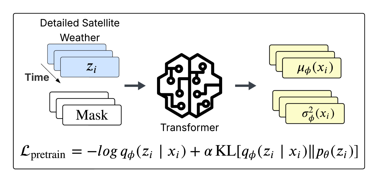
(a) Variational pretraining

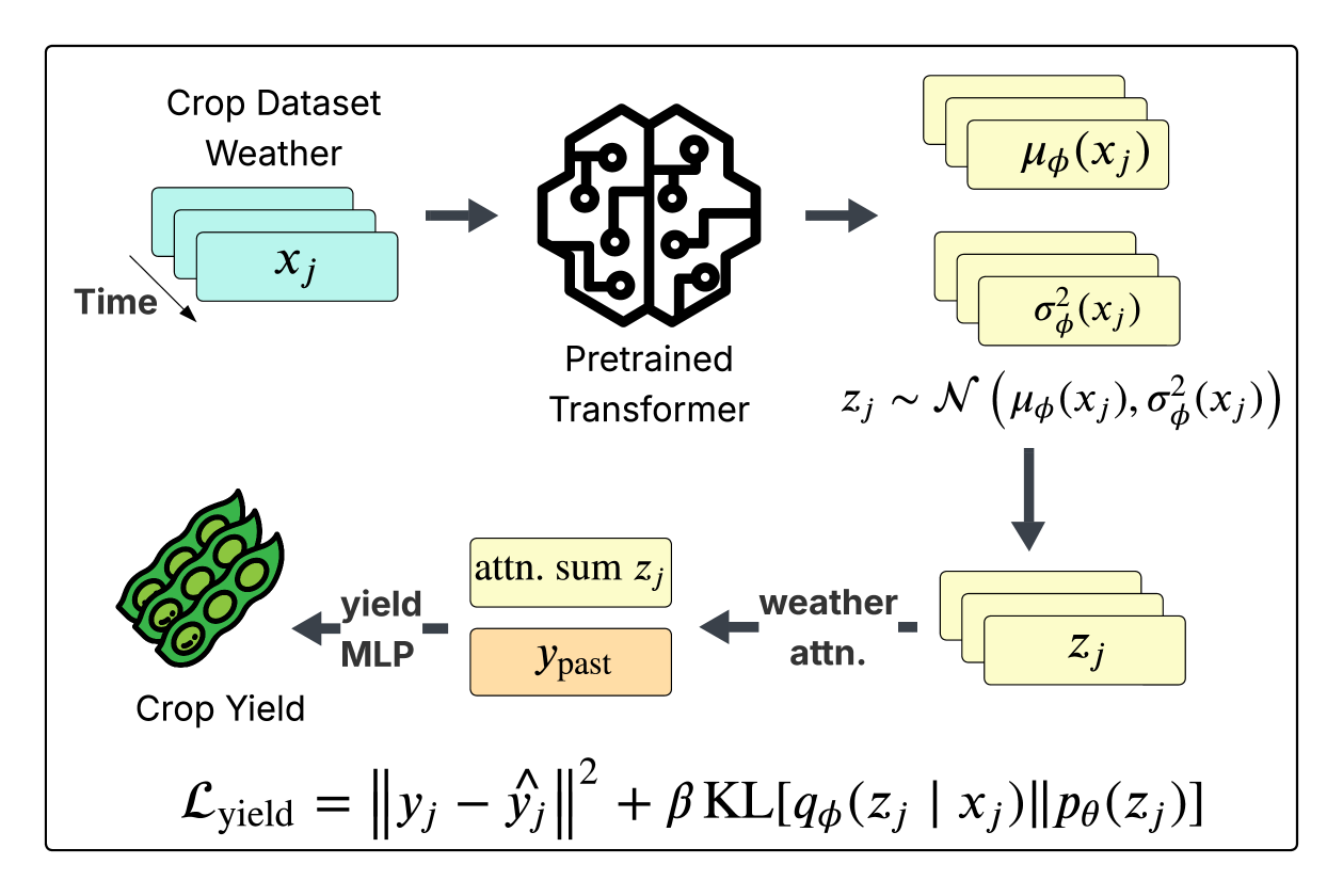
(b) Yield prediction fine-tuning

Figure 1: Two-stage variational training framework for asymmetric weather features. (a) A transformer encoder is pretrained on 31-variable weather time series by randomly masking $10\leq k\leq 25$ features and predicting them from remaining context. The model learns a variational posterior $q_{\phi}(z_{i}\mid x_{i})$ over weather representations by directly maximizing variational likelihood. (b) During fine-tuning, only 6 weather features are available. The pretrained transformer encodes these into a latent distribution $q_{\phi}(z_{j}\mid x_{j})$, from which $z_{j}\sim\mathcal{N}(\mu_{\phi}(x_{j}),\sigma_{\phi}^{2}(x_{j}))$ is sampled. It is aggregated with learnable attention across time dimension and concatenated with historical yield $y_{\text{past}}$ for final yield prediction.

Climate change is transforming global agricultural systems, with extreme weather events becoming more frequent and causing billions of dollars in annual crop losses (Lobell, Schlenker, and Costa-Roberts 2011). The 2012 U.S. drought led to a 13% reduction in national corn yields, while the 2019 Midwest flooding prevented planting on 19.4 million acres (USDA National Agricultural Statistics Service 2013; USDA Farm Service Agency 2019). Agricultural economists emphasize that accurate yield prediction under these volatile conditions is critical for food security, insurance markets, and adaptive farm management (Beddington 2010). Yet current AI models often underperform precisely when yields diverge from historical trends.

This challenge stems from fundamental data limitations that existing methods do not address. First, many models train on limited historical data spanning less than 10 years (Gandhi, Petkar, and Armstrong 2016; Lin et al. 2024), insufficient for capturing rare but increasingly critical extreme weather patterns. Second, multi-modal approaches (You et al. 2017; Lin et al. 2024; Khaki, Wang, and Archontoulis 2019; Fan et al. 2021) rely on extensive auxiliary data—satellite imagery, soil surveys, and comprehensive weather records—which limits their applicability in regions that lack detailed agricultural monitoring infrastructure.

Third, general-purpose time-series pretraining methods like SimMTM (Dong et al. 2023) and PatchTST (Wu et al. 2023) assume consistent input features between pretraining and fine-tuning. This breaks down in weather domains, where pretraining can leverage rich satellite datasets with dozens of variables (e.g., 31 meteorological variables from NASA POWER (NASA 2024)), but fine-tuning must rely on smaller, accessible subsets (e.g., 6 basic weather variables from Khaki, Wang, and Archontoulis (2019)). This data asymmetry prevents generic frameworks from fully exploiting physical interdependencies among weather variables.

We address these limitations with VITA, a novel variational pretraining framework designed for weather-yield prediction. VITA approaches the data asymmetry problem by learning representations from comprehensive weather datasets during pretraining, then transferring this knowledge to scenarios with limited weather variables during fine-tuning. Rather than reconstructing inputs like traditional variational autoencoder  VITA uses detailed weather variables as proxy targets for learning representations. This approach is justified by established meteorological principles—Tetens equation, Penman-Monteith formulations, and Clausius-Clapeyron relations (O. Tetens 1930; Ndulue and Ranjan 2021; Brown 1951; Murray-Tortarolo 2023)—which demonstrate that strong physical relationships exist between comprehensive atmospheric states and basic weather statistics. By predicting detailed weather variables from partial observations during pretraining, VITA learns representations that naturally capture these interdependencies without requiring extensive auxiliary data or consistent feature sets.

We also find that the influence of soil characteristics and farming practices on yield can be partially inferred from past 6 years of yield, enabling competitive performance using only weather and historical yield information.

VITA is a transformer-based architecture that introduces less than 2% additional parameters to a standard Transformer (Vaswani et al. 2017) and completes training in under 2.5 hours on one L40S GPU. Empirically, VITA achieves state-of-the-art performance during years with the largest yield deviations, showing statistically significant improvements ($p\approx 0.01$) over other pretraining strategies when evaluated on identical model architectures. VITA also demonstrates strong spatial transferability: models pretrained on weather data outside the continental U.S. still improve performance when fine-tuned on U.S. crop yields. Moreover, it demonstrates temporal robustness, as models trained on historical data (1994–2009) continue to achieve high accuracy when applied to data from a later period (2014–2018), without retraining.

In summary, the key contributions of this work are:

• A decoder-free variational pre-training framework for modeling asymmetric features (see Equation 4).

• A seasonality-aware sinusoidal prior that captures structured temporal patterns.

• State-of-the-art performance in years with extreme yield deviations, validated through rigorous, statistically grounded evaluation.

The remainder of this paper is organized as follows: Methodology details our variational framework, Experiments presents our experimental setup, Results analyzes performance across extreme and standard conditions, and Discussion discusses implications and limitations.

Methodology

VITA incorporates a two-stage approach: (1) self-supervised pretraining on extensive weather data to learn robust weather representations, and (2) variational fine-tuning with basic weather statistics and past yields.

Problem Formulation

Figure 2: Graphical model depicting data structure of pretraining and prediction phases in VITA.

We formulate crop yield prediction as semi-supervised learning with latent weather representations. Let $z\in\mathbb{R}^{364\times 31}$ be detailed meteorological variables from pretraining, and $x\in\mathbb{R}^{364\times 6}$ be basic weather statistics (temperature, precipitation, etc.) available in both pretraining and downstream tasks. Each weather input is 364-week sequences representing 7 years of weekly means.

We have two datasets: $\mathcal{D}_{w}=\{(x_{i},z_{i})\}_{i=1}^{N_{w}}$ where both basic and detailed weather states are observed for each 364-week non-overlapping window $i$ across the NASA POWER grid, and $\mathcal{D}_{y}=\{(x_{j},y_{j},y_{\text{past},j})\}_{j=1}^{N_{y}}$ where detailed states $z_{j}$ remain latent for each 364-week overlapping sequence $j$ across the US Corn Belt counties. Here, $N_{w}$ represents the total number of rolling windows in the pretraining dataset and $N_{y}$ represents the total number of 7-year sequences in the fine-tuning dataset.

Architecture

VITA employs a transformer-based architecture with weather encoder $E_{\phi}$ processing 364-week sequences:

$$x_{\text{input}} =\mathrm{concat}(x_{\text{weather}},\text{year},\text{coords})$$ (1)

$$h_{\text{weather}} =E_{\phi}(\text{LinearProj}(x_{\text{input}})+\text{PosEmbed}(t))$$ (2)

The encoder outputs diagonal Gaussian variational posterior parameters: $q_{\phi}(z\mid x)=\mathcal{N}(z;\mu_{\phi}(x),\text{diag}(\sigma_{\phi}^{2}(x)))$. We sample weather latent variables and aggregate using learned attention for yield prediction.

Self-Supervised Pretraining

We pretrain on NASA POWER dataset (1984-2022) using progressive feature-wise masking, starting with $k=10$ masked features and increasing by 1 every 2 epochs until 25 out of 31 features are masked. The pretraining objective balances reconstruction with regularization:

$$\mathcal{L}_{\text{pretrain}}= -\mathbb{E}_{(x_{i},z_{i})\sim\mathcal{D}_{w}}\left[\log q_{\phi}(z_{i}\mid x_{i})\right.$$

$$+\left.\alpha\cdot\text{KL}[q_{\phi}(z_{i}\mid x_{i})\|p_{\theta}(z_{i})]\right]$$

$$= -\mathbb{E}_{(x_{i},z_{i})\sim\mathcal{D}_{w}}\left[\log\mathcal{N}(z_{i};\mu_{\phi}(x_{i}),\sigma^{2}_{\phi}(x_{i}))\right]$$

$$+\alpha\cdot\text{KL}[q_{\phi}(z_{i}\mid x_{i})\|p_{\theta}(z_{i})]$$ (3)

The first term maximizes the Gaussian likelihood, which encourages the posterior distribution $q_{\phi}(z_{i}\mid x_{i})$ to accurately predict the observed detailed weather state $z_{i}$. The second term is the regularizer preventing overfitting by imposing a prior structure.

We investigate two prior distributions: standard normal $p_{\theta}(z)\sim\mathcal{N}(0,I)$ and sinusoidal prior $p_{\theta}(z)\sim\mathcal{N}(\mu_{\sin}=A\sin(\theta\cdot\text{pos}+\theta_{0}),\sigma^{2}I)$ to capture seasonal patterns. Sinusoidal prior has additional prior parameters that are learned during both pretraining and finetuning. This prior explicitly models the periodicity in weather variables, allowing a more structured latent space.

To validate that pretraining benefits arise from weather pattern learning rather than year-specific memorization, we conduct an additional ablation where calendar-year labels in the pretraining set are randomly permuted, destroying temporal relationships while preserving weather statistics (detailed results in Appendix).

Decoder-Free Fine-Tuning Objective

Standard semi-supervised VAEs include a decoder term $\log p(x_{j}|z_{j})$ to model input reconstruction (Kingma et al. 2014). However, in our meteorological context, established principles like the Tetens equation, Penman-Monteith formulation, and Stefan-Boltzmann radiation balance link basic weather statistics to the detailed atmospheric state (O. Tetens 1930; Ndulue and Ranjan 2021; Brown 1951; Murray-Tortarolo 2023), making the decoder term unnecessary.

We empirically validated this deterministic relationship, training an MLP to reconstruct basic weather variables from detailed ones with near-perfect accuracy ($R^{2}>0.9999$), justifying our decoder-free approach (see Appendix). This enables us to model $p(x_{j}|z_{j})\approx 1$ and derive the simplified variational objective:

$$\mathcal{L}_{\text{yield}}=\|y_{j}-\hat{y}_{j}\|^{2}+\beta\cdot\text{KL}[q_{\phi}(z_{j}\mid x_{j})\|p_{\theta}(z_{j})]$$ (4)

where $\beta>0$ is a hyperparameter. Note that the $\beta$ in Equation (4) does not weaken the variational objective and the full evidence lower bound (ELBO) is still optimized. The full derivation of this objective is shown in the Appendix.

Baselines

We compare against SimMTM (Dong et al. 2023), a SOTA masked time series pretraining method that faces challenges due to our asymmetric data structure. We introduce T-BERT as a rigorous non-variational baseline using identical architecture and training procedures as VITA, differing only in using standard MSE reconstruction loss without variational parameters. We also compare against linear regression, CNN-RNN (Khaki, Wang, and Archontoulis 2019), and GNN-RNN (Fan et al. 2021), with the latter two accessing comprehensive soil data while our approach uses only weather and yield data. This evaluation design ensures fair comparison by isolating the contribution of our variational pretraining approach from architectural advantages.

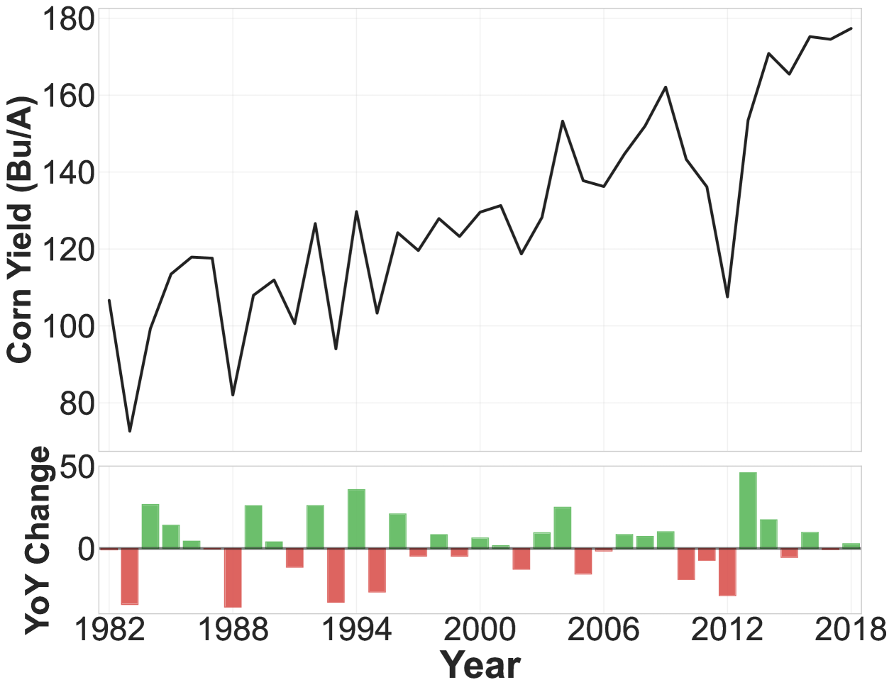
(a) Corn yield trends by year

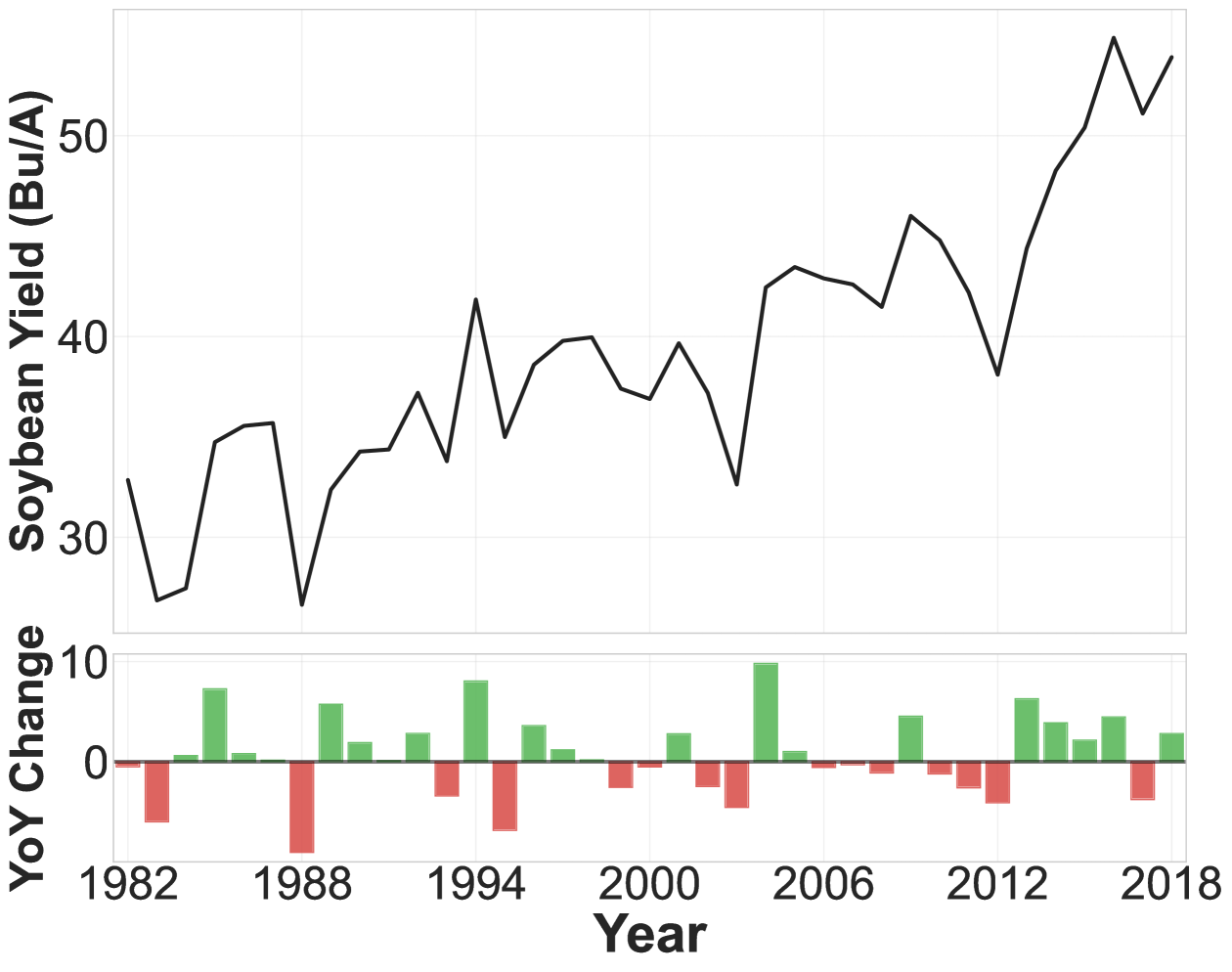
(b) Soybean yield trends by year

Figure 3: Mean crop yield across US Corn Belt counties showing extreme weather years as sharp deviations from historical patterns.

Experiments

We test three hypotheses: (1) weather pretraining improves yield prediction on extreme weather years, (2) variational objectives with sinusoidal priors outperform standard approaches, and (3) these benefits generalize to standard years and forward temporal gaps. We evaluate on county-level corn and soybean yield prediction across 763 US Corn Belt counties.

Data.

We pretrain on the NASA POWER dataset (NASA 2024) spanning 39 years (1984–2022) across 116 spatial grids at 0.5° resolution covering the Americas, providing 31 meteorological variables aggregated as weekly averages with approximately 100K temporal sequences. For yield prediction, we evaluate on county-level corn and soybean yields from 763 US Corn Belt counties (1982–2018) (Khaki, Wang, and Archontoulis 2019; U.S. Department of Agriculture, National Agricultural Statistics Service 2023). We focus on corn (C4) and soybean (C3) crops as they span distinct physiological and weather-sensitivity regimes yet together account for over 60% of U.S. row-crop acreage. (Williams and Pounds-Barnett 2024) We use only six basic weather variables (min/max temperature, solar radiation, precipitation, snow water equivalent, vapor pressure), historical yields, and county centroid coordinates, but exclude soil data to test deployment in data-sparse regions. This presents the key challenge of asymmetric feature availability (31 vs. 6 variables) that generic pretraining methods struggle to address. All data sources (NASA POWER weather data and USDA county-level yields) are resampled to weekly granularity to ensure consistent temporal resolution across pretraining and fine-tuning phases.

Training Configuration.

During pretraining, we use batch size 256, learning rate $5\times 10^{-4}$, max context length of 364, and progressive masking increasing from 10 to 25 features over 100 epochs with 10-epoch linear warmup followed by exponential decay ($\delta=0.99$). The variational objective balances reconstruction and KL terms with $\alpha=0.5$.

For yield prediction fine-tuning, we use overlapping 7-year sequences where each sequence spans years $t-6$ to $t$, generating 9 sequences per county from 15-year periods, with the model predicting yield for year $t$ using weather from all 7 years plus historical yields from years $t-6$ to $t-1$. We train for 40 epochs with 10-epoch linear warmup followed by cosine annealing, reporting the best validation RMSE across all epochs. We use a 15-year training window for extreme year and robustness experiments, and test both 15-year and 30-year windows for standard years, repeating each experiment across 5 different validation years. Both pretraining and fine-tuning experiments use random seed 1234 for reproducibility.

Hyperparameter Optimization.

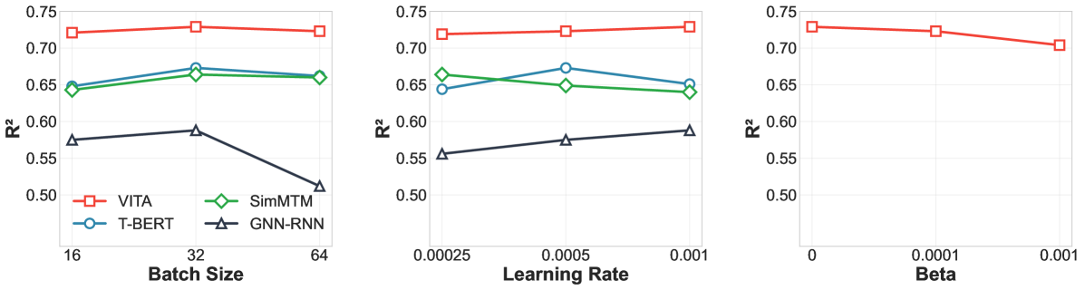
(a) Corn hyperparameter grid search

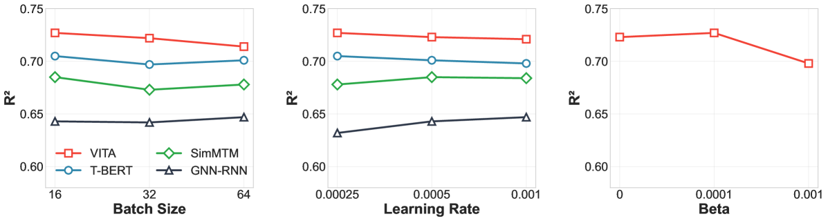
(b) Soybean hyperparameter grid search

Figure 6: Hyperparameter robustness on extreme years: VITA-Sinusoidal consistently outperforms T-BERT across all configurations tested. The CNN-RNN performs considerably worse and not shown in the plot.

We performed a 27-configuration grid search to optimize hyperparameters, with full details and robustness analysis in Appendix Figure 6. Best hyperparameters are used for all subsequent experiments.

Method	Corn	Soybean	Mean R²
	R² (RMSE)	R² (RMSE)
CNN-RNN	0.230 (27.0)	0.500 (6.7)	0.365
GNN-RNN	0.588 (19.7)	0.647 (5.6)	0.618
SimMTM	0.664 (18.3)	0.685 (5.3)	0.675
T-BERT (ours)	0.673 (18.1)	0.705 (5.1)	0.689
VITA-Std. Normal (ours)	0.734 (16.1)	0.715 (5.1)	0.725
VITA-Sinusoidal (ours)	0.729 (16.4)	0.727 (5.0)	0.728

Table 1: Performance on the 5 most extreme years per crop. Best results bolded.

Extreme Year Evaluation (Primary Contribution)

We identify the five most weather-extreme years for each crop between 2000 and 2018 by computing absolute z-scores from 5-year rolling means of yields. For each selected year, we train models on the preceding 15 years and evaluate on that year. These include known drought years (2002, 2003, 2012) and years with favorable conditions and record-breaking yields (2004, 2009). (National Drought Mitigation Center, NOAA, and USDA 2025) We focus on the five most weather-extreme years per crop because they are the hardest, policy-relevant scenarios; performance on normal and temporal-shift tests (reported below) shows the method’s generality.

Standard Years Generalization

To validate that extreme weather optimization doesn’t compromise standard performance, we evaluate on 2014–2018 using hyperparameters optimized for extreme years. We test both 15-year and 30-year training periods to assess data efficiency requirements.

Temporal Robustness

We evaluate temporal robustness across five experiments with 5-year gaps: train on 1994–2009/test on 2014, train on 1995–2010/test on 2015, and so forth through 2018.

Ablation Studies

We ablate: (1) pretraining vs. random initialization, (2) variational vs. MSE objective, (3) sinusoidal vs. normal priors, and (4) spatial generalization by pretraining on weather grids excluding continental USA, focusing on extreme weather performance.

All pretraining experiments run on four L40S GPUs and all finetuning experiments run on one L40S GPU with identical computational budgets across methods. The code, pretrained models, and datasets will be publicly released upon publication to facilitate reproducibility and broader agricultural AI research.

Results

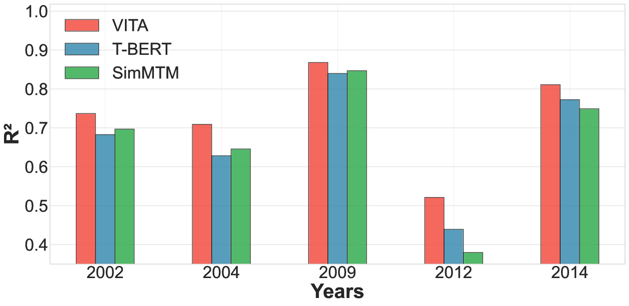
(a) Corn

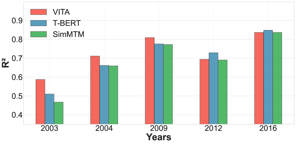
(b) Soybean

Figure 4: Individual R² comparisons on extreme years showing consistent improvements of VITA-Sinusoidal over T-BERT across all evaluation instances.

Extreme Years Performance

VITA-Sinusoidal achieves notable improvements of +0.056 (+8.3%) and +0.022 (+3.1%) over T-BERT’s 0.673 and 0.705 respectively. These gains translate to RMSE reductions of 1.7 bushels/acre for corn and 0.1 bushels/acre for soybean during the most challenging prediction scenarios.

Figure 4 demonstrates consistency across individual extreme years, with VITA outperforming T-BERT on 8/10 evaluations and SimMTM on 9/10, showing improvements ranging from +0.01 to +0.15 R². The limited underperformances occur when baseline models already achieve high accuracy (soybean 2012: 0.729 R², soybean 2016: 0.848 R²), leaving minimal room for improvement compared to scenarios with lower baseline performance like corn 2012 (0.439 R²). Statistical validation across 27 hyperparameter configurations confirms significance (paired t-test, $p\approx 0.0105$).

Critically, our weather-only approach substantially outperforms soil-enhanced methods: CNN-RNN achieves only 0.230 R² for corn and 0.500 for soybean, while GNN-RNN reaches 0.588 and 0.647 respectively, despite accessing detailed soil information. SimMTM underperforms both transformer approaches due to variable mismatch between pretraining and fine-tuning phases.

Standard Years Performance (2014–2018)

Method	Corn 15yr	Corn 30yr	Soybean 15yr	Soybean 30yr
	R² (RMSE)	R² (RMSE)	R² (RMSE)	R² (RMSE)
CNN-RNN	0.659 (20.7)	0.635 (20.8)	0.721 (5.6)	0.671 (6.0)
GNN-RNN	0.788 (16.6)	0.785 (16.5)	0.800 (4.7)	0.810 (4.6)
SimMTM	0.753 (17.9)	0.768 (17.2)	0.814 (4.6)	0.822 (4.5)
T-BERT (ours)	0.791 (16.5)	0.780 (16.8)	0.831 (4.4)	0.837 (4.3)
VITA-Sinusoidal (ours)	0.827 (16.0)	0.837 (15.5)	0.833 (4.3)	0.837 (4.2)

Table 2: Standard years performance (2014-2018 test). Best results in each column are bolded.

VITA maintains strong performance on standard years, providing consistent corn improvements over T-BERT: +0.036 R² (0.827 vs 0.791) for 15-year data and +0.057 R² (0.837 vs 0.780) for 30-year data, corresponding to RMSE reductions of 0.5 and 1.3 bushels/acre. For soybean, VITA achieves competitive performance with slight improvements: 0.833 vs 0.831 R² for 15-year data and matching 0.837 R² for 30-year data.

Notably, our weather-only approach matches or exceeds GNN-RNN performance across all scenarios despite the latter accessing detailed soil data. The smaller relative improvements compared to extreme years align with our hypothesis that uncertainty modeling provides greatest benefit when prediction conditions are most challenging.

Temporal Robustness

Method	Corn	Soybean	Mean R²
	R² (RMSE)	R² (RMSE)
CNN-RNN	0.556 (23.9)	0.659 (6.2)	0.608
GNN-RNN	0.718 (18.9)	0.785 (4.9)	0.752
SimMTM	0.705 (19.7)	0.776 (5.0)	0.741
T-BERT (ours)	0.782 (16.9)	0.803 (4.7)	0.793
VITA-Sinusoidal (ours)	0.797 (16.3)	0.819 (4.5)	0.808

Table 3: Forward gap robustness: 5-year distribution shift (train: 1994-2009, test: 2014-2018). Best results bolded.

VITA-Sinusoidal demonstrates exceptional temporal robustness, achieving R² scores of 0.797 for corn and 0.819 for soybean—improvements of +0.015 and +0.016 over T-BERT (0.782 corn, 0.803 soybean). While CNN-RNN and GNN-RNN show substantial performance degradation under temporal shift (CNN-RNN drops to 0.556 corn R², GNN-RNN to 0.718), both T-BERT and VITA maintain strong performance. SimMTM also shows notable degradation (0.705 corn, 0.776 soybean), suggesting feature-wise masking strategies in transformer architectures provide superior temporal robustness.

Ablation Studies

Pretraining Impact

Crop	Model	Pretrained	Best R²	Mean R²	t-statistic	p-value
Corn	SimMTM	No	0.604	$0.580\pm 0.010$	3.90	$<0.01$
		Yes	0.664	$0.630\pm 0.030$
	T-BERT	No	0.604	$0.584\pm 0.015$	9.13	$<0.01$
		Yes	0.673	$0.647\pm 0.014$
	VITA-Sinusoidal	No	0.672	$0.469\pm 0.227$	5.35	$<0.01$
		Yes	0.729	$0.703\pm 0.015$
	VITA-Std Normal	No	0.685	$0.574\pm 0.119$	5.44	$<0.01$
		Yes	0.734	$0.700\pm 0.020$
Soybean	SimMTM	No	0.680	$0.660\pm 0.020$	1.59	0.14
		Yes	0.685	$0.670\pm 0.010$
	T-BERT	No	0.680	$0.660\pm 0.020$	4.36	$<0.01$
		Yes	0.705	$0.693\pm 0.012$
	VITA-Sinusoidal	No	0.684	$0.569\pm 0.139$	4.80	$<0.01$
		Yes	0.727	$0.698\pm 0.019$
	VITA-Std Normal	No	0.714	$0.638\pm 0.074$	2.33	$<0.05$
		Yes	0.715	$0.672\pm 0.025$

Table 4: Pretraining effect across different hyperparameter configurations during grid search.

Weather pretraining provides substantial improvements across all transformer models. For corn, T-BERT gains +0.063 mean R² (0.647 vs 0.584), while VITA variants achieve larger gains: +0.234 (Sinusoidal) and +0.126 (Standard Normal) mean R². For soybean, improvements are more moderate: T-BERT +0.033 mean R² (0.693 vs 0.660), VITA-Sinusoidal +0.129, and VITA-Standard Normal +0.034. All improvements are statistically significant except SimMTM on soybean ($p=0.14$), consistent with corn’s higher weather sensitivity (Schauberger et al. 2017; Lobell, Schlenker, and Costa-Roberts 2011).

Spatial Transfer

Crop	Model	Pretrained	Best R²	Mean R²	t-statistic	p-value
Corn	VITA-Sinusoidal	No	0.672	$0.469\pm 0.227$	3.61	$<0.01$
		Non-US	0.658	$0.627\pm 0.020$
	VITA-Std Normal	No	0.685	$0.574\pm 0.119$	2.969	$<0.01$
		Non-US	0.687	$0.644\pm 0.031$
Soybean	VITA-Sinusoidal	No	0.684	$0.569\pm 0.139$	3.685	$<0.01$
		Non-US	0.707	$0.669\pm 0.021$
	VITA-Std Normal	No	0.714	$0.638\pm 0.074$	2.774	$<0.01$
		Non-US	0.703	$0.678\pm 0.019$

Table 5: Pretraining effects on non-US weather grids.

Pretraining on Central and South American weather (Excluding continental US weather) also significantly improves US corn belt crop yield prediction. For corn, improvements are +0.158 mean R² (0.627 vs 0.469) for VITA-Sinusoidal and +0.070 (0.644 vs 0.574) for VITA-Standard Normal. For soybean, gains are +0.100 (0.669 vs 0.569) and +0.040 (0.678 vs 0.638) respectively. All improvements are statistically significant ($p<0.01$) with dramatically reduced variance across hyperparameter configurations, demonstrating that VITA learns generalizable weather-agriculture relationships that transcend geographic boundaries.

Discussion

Our variational weather pretraining framework achieves consistent improvements in crop yield prediction, with statistically significant gains over architecturally identical T-BERT baselines (paired t-test, $p\approx 0.0105$). These benefits are most pronounced during extreme weather conditions, precisely when accurate predictions are most critical.

Extreme Year Performance.

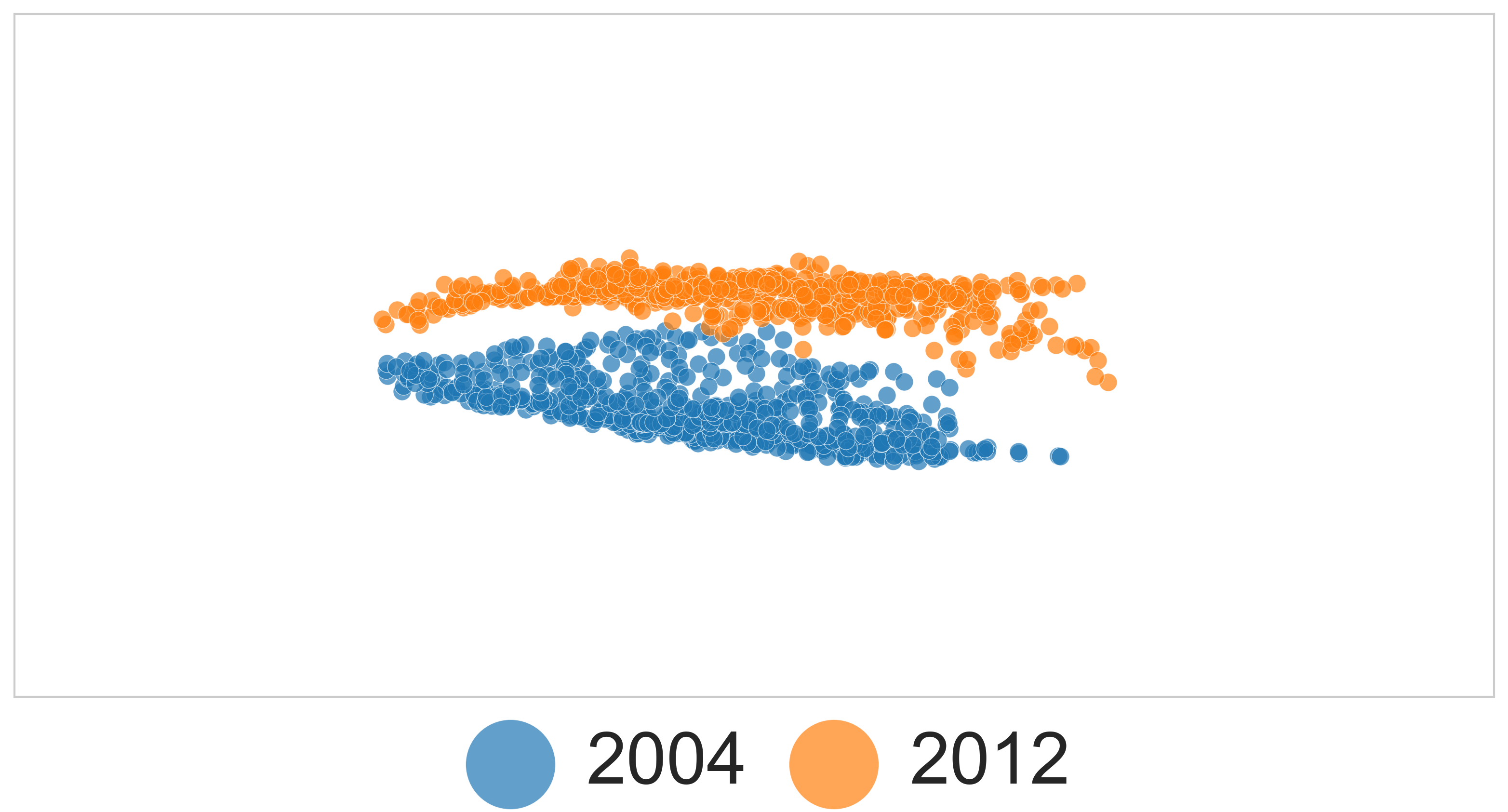
(a) T-BERT (84.0%)

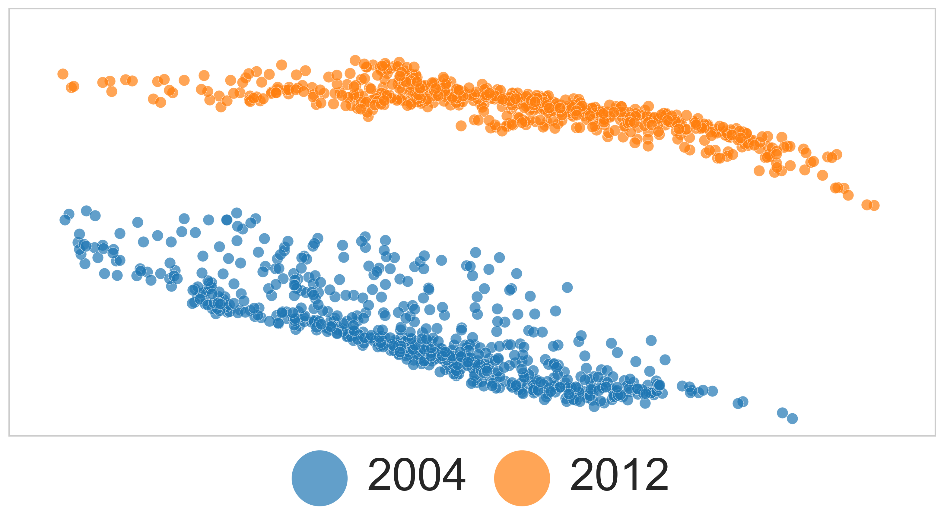
(b) Standard normal prior (37.7%)

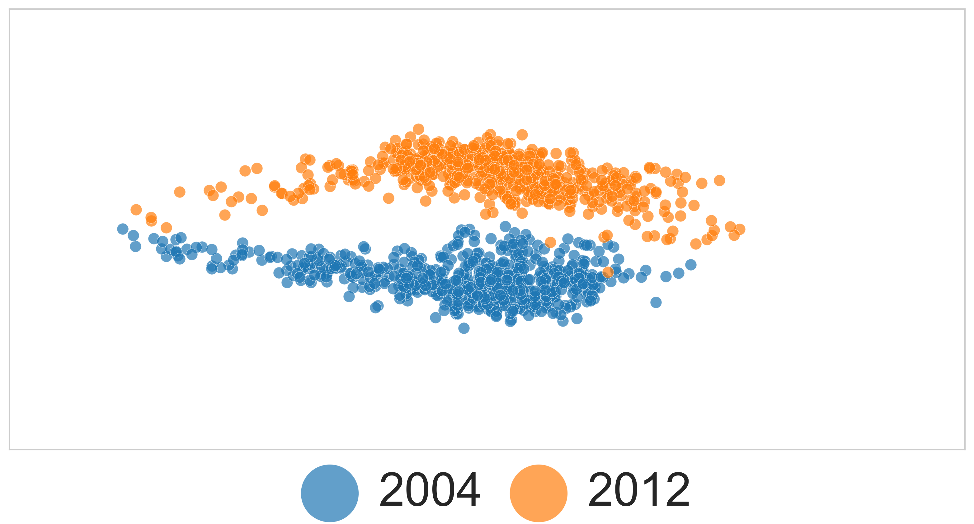
(c) Sinusoidal prior (15.7%)

Figure 5: PCA visualization of the latent weather representations for two extreme years (2004: record-breaking yield, 2012: extreme drought) under different modeling choices. (a) T-BERT (non-variational) shows limited separation and explains 84.0% of variance in 2D, reflecting a narrow, collapsed latent space. (b) VITA with a standard normal prior yields more separated clusters and explains 34.7% of variance. (c) Sinusoidal prior induces visually tighter clusters but with only 15.7% explained variance, indicating even spread of variance into higher-order components.

VITA’s superior performance during extreme years can be attributed to its rich latent space learned with the variational objective. The latent space analysis also supports this: in Figure 5, VITA with sinusoidal prior avoids latent space collapse seen in T-BERT (15.7% vs. 84.0% variance in the top two components), indicating richer weather representations that differentiate between normal and extreme conditions.

Competitive Performance Without Soil Data.

VITA’s ability to match or exceed GNN-RNN performance despite lacking soil information suggests that historical yield patterns act as an effective proxy for soil and management practices when combined with rich weather representations.

Variational Framework Benefits.

The decoder-free variational objective leverages deterministic relationships between basic and detailed meteorological variables, allowing the model to focus learning capacity on yield prediction rather than weather reconstruction. The sinusoidal prior’s superior performance reflects its alignment with seasonal agricultural systems.

Ethical & Societal Impact.

VITA’s open-source code and publicly available datasets minimize ethical risks through transparency and reproducibility. Data privacy concerns are negligible as we use aggregated meteorological data without individual farm records. While speculative trading remains a theoretical concern, the public availability of both methods and data ensures equitable access to information. The framework’s reliance on standard weather stations and consumer-grade hardware specifically addresses distributive effects.

Facilitating Follow-up Work.

We commit to open-sourcing our complete implementation, including preprocessing scripts, model architectures, and trained weights. Both the pretraining and the fine-tuning dataset are publicly available, and we will release clear documentation for adaptation to new regions. Furthermore, because our derivation only assumes a deterministic mapping $x\leftarrow z$, the same variational recipe applies to any setting with rich sensors at training time and sparse sensors at inference (e.g. ICU vitals vs. high-resolution labs, or low-cost IoT vs. full industrial telemetry). We leave empirical validation in such domains to future work.

Limitations.

Our evaluation is limited to corn and soybean yields in the U.S. Corn Belt, aligning with prior benchmarks (Khaki, Wang, and Archontoulis 2019; Fan et al. 2021). While pretraining on broader weather data from the Americas shows promising transferability, extending this approach to other crops and global regions remains an important direction for future work.

Conclusion

We introduced VITA, a variational pretraining framework that addresses critical challenges in agricultural forecasting for global food security. By leveraging meteorological domain knowledge through decoder-free variational learning and seasonality-aware priors, VITA achieves state-of-the-art performance on extreme weather years (R² = 0.729 for corn, 0.727 for soybeans) when accurate predictions are most critical. The framework requires only basic weather variables available globally, allowing deployment in data-scarce regions where multi-modal approaches are infeasible. Our comprehensive evaluation across 763 US Corn Belt counties with statistical validation and spatial transfer experiments, demonstrates robust performance. With open-source code and reproducible methodology, VITA provides a scalable approach for AI-driven food security.

Related Work

Crop Yield Prediction.

Agricultural yield forecasting leverages multiple data modalities through CNN-RNN architectures, graph neural networks, Deep Gaussian Processes, and Vision Transformers (Khaki, Wang, and Archontoulis 2019; Fan et al. 2021; You et al. 2017; Lin et al. 2024). Multi-modal approaches integrate satellite imagery, weather data, soil surveys, management records, and vegetation indices (Wu et al. 2021; Sun et al. 2019; Gandhi, Petkar, and Armstrong 2016; Oliveira et al. 2018; Basir et al. 2021; Ferraz et al. 2024; Cao, Ma, and Zhang 2022). However, extensive data requirements limit deployment in regions with limited agricultural monitoring infrastructure, and many approaches rely on short regional datasets that may not capture sufficient weather variability for extreme events (Gandhi, Petkar, and Armstrong 2016; Lin et al. 2024; McFarland et al. 2020; Chu and Yu 2020).

Time Series Pretraining.

Recent work develops unsupervised representation learning through contrastive methods, transformer frameworks, and masked reconstruction (Franceschi, Dieuleveut, and Jaggi 2019; Yue et al. 2022; Zerveas et al. 2021; Dong et al. 2023; Wu et al. 2023; Woo et al. 2022). These methods achieve strong forecasting performance but do not explicitly model feature asymmetry, which is critical for agricultural data.

Variational Methods.

Variational autoencoders and their extensions have been applied to weather prediction, climate forecasting, and agricultural data generation (Kingma and Welling 2013; Higgins et al. 2017; Kwok and Qi 2021; Wang et al. 2024; Palma et al. 2025; Razavi et al. 2024). However, existing variational methods in meteorology predominantly learn from input reconstruction, and are not used for asymmetric data tasks. Our work is applicable for this particular problem and learns latent state from direct variational distribution likelihood maximization and with a seasonal-aware sinusoidal prior.

Reproducibility Checklist

 

Instructions for Authors:

This document outlines key aspects for assessing reproducibility. Please provide your input by editing this .tex file directly.

For each question (that applies), replace the “Type your response here” text with your answer.

Example: If a question appears as

\question{Proofs of all novel claims are included} {(yes/partial/no)}
Type your response here

you would change it to:

\question{Proofs of all novel claims are included} {(yes/partial/no)}
yes

Please make sure to:

• Replace ONLY the “Type your response here” text and nothing else.

• Use one of the options listed for that question (e.g., yes, no, partial, or NA).

• Not modify any other part of the \question command or any other lines in this document.
  

You can \input this .tex file right before \end{document} of your main file or compile it as a stand-alone document. Check the instructions on your conference’s website to see if you will be asked to provide this checklist with your paper or separately.

 

1. General Paper Structure

• Includes a conceptual outline and/or pseudocode description of AI methods introduced (yes/partial/no/NA) Yes

• Clearly delineates statements that are opinions, hypothesis, and speculation from objective facts and results (yes/no) Yes

• Provides well-marked pedagogical references for less-familiar readers to gain background necessary to replicate the paper (yes/no) Yes

2. Theoretical Contributions

• Does this paper make theoretical contributions? (yes/no) Yes

  If yes, please address the following points:

  • All assumptions and restrictions are stated clearly and formally (yes/partial/no) Yes

  • All novel claims are stated formally (e.g., in theorem statements) (yes/partial/no) Yes

  • Proofs of all novel claims are included (yes/partial/no) Yes

  • Proof sketches or intuitions are given for complex and/or novel results (yes/partial/no) Yes

  • Appropriate citations to theoretical tools used are given (yes/partial/no) Yes

  • All theoretical claims are demonstrated empirically to hold (yes/partial/no/NA) Yes

  • All experimental code used to eliminate or disprove claims is included (yes/no/NA) NA

3. Dataset Usage

• Does this paper rely on one or more datasets? (yes/no) Yes

  If yes, please address the following points:

  • A motivation is given for why the experiments are conducted on the selected datasets (yes/partial/no/NA) Yes

  • All novel datasets introduced in this paper are included in a data appendix (yes/partial/no/NA) Yes

  • All novel datasets introduced in this paper will be made publicly available upon publication of the paper with a license that allows free usage for research purposes (yes/partial/no/NA) Yes

  • All datasets drawn from the existing literature (potentially including authors’ own previously published work) are accompanied by appropriate citations (yes/no/NA) Yes

  • All datasets drawn from the existing literature (potentially including authors’ own previously published work) are publicly available (yes/partial/no/NA) Yes

  • All datasets that are not publicly available are described in detail, with explanation why publicly available alternatives are not scientifically satisficing (yes/partial/no/NA) NA

4. Computational Experiments

• Does this paper include computational experiments? (yes/no) Yes

  If yes, please address the following points:

  • This paper states the number and range of values tried per (hyper-) parameter during development of the paper, along with the criterion used for selecting the final parameter setting (yes/partial/no/NA) Yes

  • Any code required for pre-processing data is included in the appendix (yes/partial/no) Yes

  • All source code required for conducting and analyzing the experiments is included in a code appendix (yes/partial/no) Yes

  • All source code required for conducting and analyzing the experiments will be made publicly available upon publication of the paper with a license that allows free usage for research purposes (yes/partial/no) Yes

  • All source code implementing new methods have comments detailing the implementation, with references to the paper where each step comes from (yes/partial/no) Yes

  • If an algorithm depends on randomness, then the method used for setting seeds is described in a way sufficient to allow replication of results (yes/partial/no/NA) Yes

  • This paper specifies the computing infrastructure used for running experiments (hardware and software), including GPU/CPU models; amount of memory; operating system; names and versions of relevant software libraries and frameworks (yes/partial/no) Yes

  • This paper formally describes evaluation metrics used and explains the motivation for choosing these metrics (yes/partial/no) Yes

  • This paper states the number of algorithm runs used to compute each reported result (yes/no) Yes

  • Analysis of experiments goes beyond single-dimensional summaries of performance (e.g., average; median) to include measures of variation, confidence, or other distributional information (yes/no) Yes

  • The significance of any improvement or decrease in performance is judged using appropriate statistical tests (e.g., Wilcoxon signed-rank) (yes/partial/no) Yes

  • This paper lists all final (hyper-)parameters used for each model/algorithm in the paper’s experiments (yes/partial/no/NA) Yes

Appendix

Mathematical Framework

We define $z\in\mathbb{R}^{364\times 31}$ as the full set of meteorological variables available during pretraining—such as radiation fluxes, humidity, wind speed, and surface pressure—which together describe the latent physical state of the atmosphere over 364-week sequences (7 years of weekly means). The observed variables $x\in\mathbb{R}^{364\times 6}$ are a subset of basic weather statistics used in downstream tasks, including quantities like precipitation, and min/max temperature. For brevity, in the following mathematical derivations, we use $d_{z}=364\times 31$ and $d_{x}=364\times 6$ to represent the flattened dimensions. We have two datasets: (1) A large pretraining weather dataset $\mathcal{D}_{w}=\{(x_{i},z_{i})\}_{i=1}^{N_{w}}$ where both basic weather variables $x_{i}$ and detailed weather states $z_{i}$ are observed, and (2) A crop yield dataset $\mathcal{D}_{y}=\{(x_{j},y_{j})\}_{j=1}^{N_{y}}$ where only basic weather variables $x_{j}$ and yield targets $y_{j}$ are observed, but detailed weather states $z_{j}$ remain unobserved. Our goal is to predict crop yield $y_{j}$ given basic weather variables $x_{j}$ by learning the detailed weather representation $z_{j}$ during the pretraining phase. Figure 2 shows a graphical model of the setup.

A key insight of our framework is the structured relationship between the detailed meteorological state $z$ (e.g., radiation fluxes, humidity) and the basic weather statistics $x$ (e.g., temperature, vapor pressure) used for the downstream task. Many variables in $x$ can be closely approximated or deterministically computed from components in $z$ via our deterministic-decoder assumption.

Inspired by this, we adopt the structural modeling assumption that $p_{\theta}(x\mid z)\approx 1$ for valid pairs. While not strictly true for all possible weather variables, this is a meteorologically-grounded modeling assumption that is reasonable for our dataset. This assumption allows us to eliminate the decoder term in the variational objective.

Pretraining Objective

During pretraining, paired observations $(x_{i},z_{i})\in\mathcal{D}_{w}$ can be directly used to fit the likelihood function of $q_{\phi}(z_{i}|x_{i})$. However, naively fitting likelihood leads to posterior collapse and an overconfident encoder. We therefore employ $\beta$-VAE style objective (Higgins et al. 2017) that balances reconstruction fidelity with regularization:

$$\mathcal{L}_{\text{pretrain}} =-\mathbb{E}_{(x_{i},z_{i})\sim\mathcal{D}_{w}}\Big[\log q_{\phi}(z_{i}\mid x_{i})$$

$$\quad+\alpha\,\text{KL}[q_{\phi}(z_{i}\mid x_{i})\|p_{\theta}(z_{i})]\Big]$$ (5)

where $\alpha>0$ controls regularization strength. The first term encourages accurate prediction of observed detailed weather states, while the KL term prevents posterior collapse and trains the prior parameters $\theta$.

Fine-tuning Objective

Next we derive the variational lower bound for the crop yield prediction. For each sample $(x_{j},y_{j})\in\mathcal{D}_{y}$, the log-likelihood is:

$$\log p_{\theta}(y_{j}\mid x_{j})=\log\int p_{\theta}(y_{j}\mid z_{j})p_{\theta}(z_{j}\mid x_{j})dz_{j}$$ (6)

Applying Jensen’s inequality with variational distribution $q_{\phi}(z_{j}\mid x_{j})$:

$$\log p_{\theta}(y_{j}\mid x_{j}) \geq\mathbb{E}_{q_{\phi}(z_{j}\mid x_{j})}[\log p_{\theta}(y_{j}\mid z_{j})]$$

$$\quad-\text{KL}[q_{\phi}(z_{j}\mid x_{j})\|p_{\theta}(z_{j}\mid x_{j})]$$ (7)

Using Bayes’ rule: $p_{\theta}(z_{j}\mid x_{j})=\frac{p_{\theta}(x_{j}\mid z_{j})p_{\theta}(z_{j})}{p_{\theta}(x_{j})}$ on the KL-Divergence and ignoring constants, we derive the standard semi-supervised VAE objective (Kingma et al. 2014):

$$\log p_{\theta}(y_{j}\mid x_{j}) \geq\mathbb{E}_{q_{\phi}(z_{j}\mid x_{j})}[\log p_{\theta}(y_{j}\mid z_{j})]$$

$$\quad+\mathbb{E}_{q_{\phi}(z_{j}\mid x_{j})}[\log p_{\theta}(x_{j}\mid z_{j})]$$

$$\quad-\text{KL}[q_{\phi}(z_{j}\mid x_{j})\|p_{\theta}(z_{j})]$$ (8)

Since by assumption, the detailed weather state $z_{j}$ deterministically generates basic weather statistics $x_{j}$, we have $p_{\theta}(x_{j}\mid z_{j})=1$ for valid pairs. This eliminates the decoder term $\mathbb{E}_{q_{\phi}(z_{j}\mid x_{j})}[\log p_{\theta}(x_{j}\mid z_{j})]$, yielding:

$$\mathcal{L}_{\text{yield}} =-\mathbb{E}_{q_{\phi}(z_{j}\mid x_{j})}[\log p_{\theta}(y_{j}\mid z_{j})]$$

$$\quad+\text{KL}[q_{\phi}(z_{j}\mid x_{j})\|p_{\theta}(z_{j})]$$ (9)

This loss is computed by first sampling $z_{j}\sim q_{\phi}(z_{j}|x_{j})$ with the reparameterization trick (Kingma and Welling 2013) and passed to the yield head for yield prediction.

Distributional Assumptions and Prior Choices

We assume the variational posterior $q_{\phi}(z\mid x)$ to be a diagonal Gaussian whose parameters are predicted by a transformer encoder:

$$q_{\phi}(z\mid x) =\mathcal{N}(z;\mu_{\phi}(x),\text{diag}(\sigma_{\phi}^{2}(x)))$$ (10)

The choice of prior $p_{\theta}(z)$ depends on the task structure. While standard VAEs (Kingma and Welling 2013; Kingma et al. 2014) use unit normal priors, weather data exhibits temporal patterns that motivate more sophisticated choices.

Standard Gaussian Prior.

The simplest choice is $p_{\theta}(z)=\mathcal{N}(0,I)$.

Sinusoidal Prior.

To capture seasonal patterns:

$$p_{\theta}(z) =\mathcal{N}(\mu_{\text{sin}},\text{diag}(\sigma_{\text{sin}}^{2}))$$ (11)

$$\mu_{\text{sin},k} =A_{k}\sin(\theta_{k}\cdot\text{pos}+\theta_{0,k})$$ (12)

where parameters $A_{k}$, $\theta_{k}$, $\theta_{0,k}$, and $\sigma_{\text{sin},k}^{2}$ are learned during pretraining for each dimension $k$.

Gaussian Mixture Prior.

While not explored in this paper, a sophisticated prior to capture more complex temporal weather patterns for other fine-tuning tasks could be:

$$p_{\theta}(z)=\sum_{j=1}^{K}w_{j}\mathcal{N}(\mu_{j,\text{sin}},\text{diag}(\sigma_{j,\text{sin}}^{2}))$$ (13)

In this case, the KL term in the loss has no closed form formula and will require Monte Carlo sampling via the reparameterization trick.

Yield Distribution.

Crop yield depends not only on the current year’s weather representation $z_{j}$ but also on historical yield patterns $y_{\text{past},j}$ that capture local soil conditions, management practices, and cultivar effects. For continuous yield targets $y_{j}$, we assume:

$$p_{\theta}(y_{j}\mid z_{j}) =\mathcal{N}\big(y_{j};\mu_{\theta}(z_{j},y_{\text{past},j}),\sigma_{y}^{2}\big)$$ (14)

where $\mu_{\theta}(z_{j},y_{\text{past},j})$ is the mean yield predicted by a neural network with parameters $\theta$, and $\sigma_{y}^{2}$ is a noise hyperparameter.

Practical Fine-tuning Objective

Substituting the yield likelihood (Equation (14)) into the variational lower bound (Equation (9)):

$$\mathcal{L}_{\text{yield}} =-\mathbb{E}_{q_{\phi}(z_{j}\mid x_{j})}[\log p_{\theta}(y_{j}\mid z_{j})]$$

$$\quad+\text{KL}[q_{\phi}(z_{j}\mid x_{j})\|p_{\theta}(z_{j})]$$

$$=\mathbb{E}_{q_{\phi}(z_{j}\mid x_{j})}\Big[\frac{1}{2\sigma_{y}^{2}}(y_{j}-\mu_{\theta}(z_{j},y_{\text{past},j}))^{2}\Big]$$

$$\quad+\text{KL}[q_{\phi}(z_{j}\mid x_{j})\|p_{\theta}(z_{j})]+C$$ (15)

where $C$ is a constant. Dropping constants and absorbing $\frac{1}{2\sigma_{y}^{2}}$ into the hyperparameter $\beta$:

$$\mathcal{L}_{\text{yield}} =\|y_{j}-\hat{y_{j}}\|^{2}+\beta\cdot\text{KL}[q_{\phi}(z_{j}\mid x_{j})\|p_{\theta}(z_{j})]$$ (16)

where $\hat{y_{j}}=\mathbb{E}_{q_{\phi}(z_{j}\mid x_{j})}[\mu_{\theta}(z_{j},y_{\text{past},j})]$ is the predicted yield. Note that Equation (16) is still the variational lower bound and the $\beta$ multiplyer does not originate from the weakening of the variational objective.

KL Divergence Computation

For practical implementation, we need to compute the KL divergence term $\text{KL}[q_{\phi}(z_{j}\mid x_{j})\|p_{\theta}(z_{j})]$ in both the pretraining and fine-tuning objectives. If both distributions are diagonal Gaussians, this has a closed form.

Standard Gaussian Prior.

When $p_{\theta}(z)=\mathcal{N}(0,I)$ and $q_{\phi}(z\mid x)=\mathcal{N}(\mu_{\phi}(x),\text{diag}(\sigma_{\phi}^{2}(x)))$:

$$\text{KL}[q_{\phi}(z\mid x)\|p_{\theta}(z)] =\frac{1}{2}\sum_{k=1}^{d_{z}}\Big[\sigma_{\phi,k}^{2}(x)+\mu_{\phi,k}^{2}(x)-1$$

$$\quad-\log\sigma_{\phi,k}^{2}(x)\Big]$$ (17)

Sinusoidal Prior.

When $p_{\theta}(z)=\mathcal{N}(\mu_{\text{sin}},\text{diag}(\sigma_{\text{sin}}^{2}))$ with $\mu_{\text{sin},k}=A_{k}\sin(\theta_{k}\cdot\text{pos}+\theta_{0,k})$:

$$\text{KL}[q_{\phi}(z\mid x)\|p_{\theta}(z)] =\frac{1}{2}\sum_{k=1}^{d_{z}}\Big[\frac{\sigma_{\phi,k}^{2}(x)}{\sigma_{\text{sin},k}^{2}}$$

$$\quad+\frac{(\mu_{\phi,k}(x)-\mu_{\text{sin},k})^{2}}{\sigma_{\text{sin},k}^{2}}$$

$$\quad-1-\log\frac{\sigma_{\phi,k}^{2}(x)}{\sigma_{\text{sin},k}^{2}}\Big]$$ (18)

Gaussian Mixture Prior.

For the mixture prior $p_{\theta}(z)=\sum_{j=1}^{K}w_{j}\mathcal{N}(\mu_{j,\text{sin}},\text{diag}(\sigma_{j,\text{sin}}^{2}))$, the KL divergence has no closed form and requires Monte Carlo estimation:

$$\text{KL}[q_{\phi}(z\mid x)\|p_{\theta}(z)] \approx\frac{1}{L}\sum_{l=1}^{L}\Big[\log q_{\phi}(z^{(l)}\mid x)$$

$$\quad-\log p_{\theta}(z^{(l)})\Big]$$ (19)

where $z^{(l)}\sim q_{\phi}(z\mid x)$ are samples obtained via the reparameterization trick.

Latent Space Analysis

To understand how different priors affect the learned weather representations, we analyze the latent space structure using Principal Component Analysis (PCA) on two extreme years: 2004 (exceptionally good weather with record-breaking yield) and 2012 (record drought with exceptionally bad yield).

We observe distinct latent structures across models. T-BERT, trained without a prior, shows a highly compressed latent space, with 84.0% of total variance captured by just two principal components and minimal separation between years—indicating limited representational flexibility. The standard normal prior introduces posterior diversity and improves year-wise separation, but most variance is still concentrated along the x axis (25.6%), suggesting the model may be over-regularized, relying heavily on one latent direction while underutilizing others. In contrast, the sinusoidal prior results in only 15.7% of variance explained by the top two components (14.0% and 1.7%), despite having a tighter clustering. This suggests the sinusoidal model makes more effective use of the full latent space, distributing information more evenly and yielding richer latent space. These findings indicate that sinusoidal priors can enforce structure without excessive compression, supporting richer representations.

Hyperparameter Robustness Analysis

We conduct comprehensive grid search over learning rates $\{2.5\times 10^{-4},5\times 10^{-4},1\times 10^{-3}\}$, batch sizes $\{16,32,64\}$, and $\beta\in\{0,10^{-4},10^{-3}\}$, optimizing for extreme weather performance across all 27 configurations. This systematic evaluation demonstrates that VITA’s performance gains are robust across hyperparameter choices and not artifacts of specific tuning decisions.

The grid search results show that VITA-Sinusoidal consistently outperforms T-BERT across all tested configurations, with performance improvements ranging from +0.01 to +0.15 in R² across different hyperparameter combinations. This robustness is crucial for demonstrating that the methodological improvements are fundamental rather than dependent on careful hyperparameter selection.

Statistical Significance Analysis

Crop	Year	T-BERT	VITA-Sinusoidal
		R²	R²
Corn	2002	0.683	0.737
	2004	0.628	0.709
	2009	0.840	0.868
	2012	0.439	0.521
	2014	0.772	0.811
Soybean	2003	0.510	0.587
	2004	0.662	0.711
	2009	0.776	0.809
	2012	0.729	0.694
	2016	0.848	0.836
Mean		0.687	0.727

Table 6: Detailed R² performance on extreme years for statistical analysis.

To rigorously assess the statistical significance of performance improvements, we conduct both parametric and non-parametric statistical tests on the extreme years evaluation results.

Table 6 presents the complete R² scores for each extreme year and crop, comparing BERT and VITA-Sinusoidal performance.

Statistical Tests.

Paired t-test on the 10 extreme year comparisons: $t=3.24$, $p=0.010$ (two-tailed, $df=9$). Furthermore, permutation test with 10,000 iterations: $p=0.019$ (two-tailed).

Both tests confirm statistically significant improvement of VITA over T-BERT.

Year-Permutation Ablation Study

Crop	Prior	No-Pre.	Pre.
		Best R²	Best R²	$\Delta$
Corn	Std-Norm.	$0.685$	$0.732$	+0.047
	Sinusoidal	$0.672$	$0.708$	+0.036
Soybean	Std-Norm.	$0.687$	$0.717$	+0.030
	Sinusoidal	$0.684$	$0.715$	+0.031

Table 7: Year-permutation ablation on corn and soybean yield prediction. Pretraining benefits persist even when temporal relationships are destroyed.

A potential concern with our full-archive pretraining approach is that the model might memorize year-specific weather patterns rather than learning generalizable weather representations. To address this, we conduct an ablation study where we randomly permute the calendar-year labels in the pretraining dataset (1984-2022) while keeping all weather measurements unchanged. This destroys any temporal relationship between years and their corresponding weather patterns, forcing the model to rely solely on weather statistics rather than year-specific memorization.

Without changing any hyperparameters (same $\beta$, learning rate, batch size as in Table 1), pretraining still provides $\geq+0.03$ improvements, demonstrating that the benefits arise from learning weather representations rather than temporal memorization (Table 7).

Notably, the sinusoidal prior shows reduced performance gains compared to the standard normal prior in the permuted setting (corn: +0.036 vs +0.060; soybean: +0.031 vs +0.030). This degradation occurs because the sinusoidal prior imposes a sine-wave structure over temporal sequences to capture seasonal patterns. When years are randomly permuted, this temporal structure is destroyed, making the seasonal-aware prior counterproductive compared to the structure-agnostic standard normal prior.

This result validates that VITA’s pretraining benefits stem from learning robust weather pattern representations rather than exploiting temporal correlations or year-specific memorization effects, while also confirming that the sinusoidal prior’s advantages depend on preserved temporal structure.

Component	Input	Hidden	Output
Weather Input Proj.	$34$	-	$200$
Transformer ($\times 4$)	$200$	$800$	$200$
Weather Output Proj.	$200$	$-$	$31\times 2$
Weather Attention	$31$	$16$	$1$
Yield MLP	$36$	$120$	$1$
Sine Prior Param.	-	-	$124\times 364$

Table 8: VITA Model Architecture

Extreme Years Selection

Method	Pretraining	Fine-tuning
	$4\times$ L40S	$1\times$ L40S
CNN-RNN	N/A	8.58 ± 0.04 min
GNN-RNN	N/A	7.13 ± 0.03 min
SimMTM	32.56 min	25.92 ± 0.01 min
T-BERT	27.42 min	24.69 ± 0.13 min
VITA-Sinusoidal	29.21 min	25.53 ± 0.58 min

Table 9: Runtime comparison.

Crop	Year	Yield (Bu/Acre)	5-Year Mean	Deviation %	Abs. Z-Score
Corn	2004	153.25	126.21	21.42	5.25
	2012	107.55	147.64	27.15	4.08
	2009	162.09	144.78	11.96	2.21
	2002	118.71	126.32	6.03	1.58
	2014	170.83	140.52	21.58	1.45
Soybean	2009	46.01	42.57	8.07	4.72
	2003	32.63	38.22	14.63	3.81
	2012	38.10	43.41	12.24	2.78
	2004	42.44	36.75	15.48	2.23
	2016	54.88	44.67	22.85	2.09

Table 10: Top 5 extreme years selection based on yield deviation from 5-year rolling mean.

Table 10 shows the methodology for identifying extreme weather years used in our evaluation. Years are ranked by their standardized deviation (z-score) from the 5-year rolling mean yield. The top 5 years with the highest absolute z-scores for each crop were selected as extreme years for evaluation.

The z-score calculation captures both positive and negative deviations from historical norms, ensuring our evaluation includes years with both exceptionally high and low yields relative to local climatological expectations.

VITA Architecture Details

The transformer encoder uses 4 layers with 10 attention heads, hidden dimension $d_{h}=200$, and MLP dimension $d_{\text{mlp}}=800$. Its maximum context length is 364 weeks (7 years). For all MLPs, we use a GELU (Hendrycks and Gimpel 2023) activation function. The sinusoid prior requires four parameters per weather variable, and one for each length up to max length of 364.

Runtime Analysis

VITA’s variational objective adds minimal computational cost, with a fine-tuning overhead of only 3.4% compared to the non-variational T-BERT baseline (25.53 vs 24.69 minutes). Our decoder-free framework provides statistically significant improvements with minimal overhead.

Notably, SimMTM requires more pretraining time (32.56 min vs 27-29 min) due to its complicated masking strategy that involves sophisticated temporal mask generation and reconstruction. In contrast, both VITA and T-BERT employ simple feature-wise masking, making them more computationally efficient during the pretraining phase.

Since pretraining on 4×L40S GPUs takes approximately 27-29 minutes, we extrapolate that single-GPU pretraining would require approximately 108-116 minutes (4 × 27-29 min). Adding the fine-tuning time of approximately 25 minutes, the total pipeline would take approximately 133-141 minutes on a single L40S GPU, completing in under 2.5 hours.

For the hyperparameter robustness analysis, each individual experiment (one hyperparameter configuration for one crop) takes approximately 25-26 minutes for fine-tuning. Running the full grid search of 27 configurations across 2 crops requires 54 individual experiments, totaling approximately 22.5-23.4 hours of fine-tuning time across all configurations.

Empirical Determinism of Basic Features

Feature	Best RMSE	$R^{2}$
Feature 1	0.01623	0.99993
Feature 2	0.01655	0.99995
Feature 3	0.01544	0.99990
Feature 4	0.01605	0.99990
Feature 5	0.01502	0.99991
Feature 6	0.01584	0.99994

Table 11: Reconstruction accuracy of the six basic weather features on the validation set.

As described previously, each weather token $z_{i,t}\in\mathbb{R}^{31}$ contains both the 25 unobserved meteorological variables and the 6 basic weather statistics $x_{i,t}$ (e.g., max/min temperature, precipitation) used in downstream tasks. To justify modeling $p_{\theta}(x\mid z)\approx 1$ and dropping the decoder term from the variational objective, we empirically verify that the 6 basic features are deterministic functions of the 25 detailed components in the pretraining dataset.

Experimental Setup.

Let $u_{j}\in\mathbb{R}^{25\times 52}$ denote the detailed meteorological variables over 52 weeks, and $x_{j}\in\mathbb{R}^{6\times 52}$ the corresponding basic weather statistics. We train a lightweight neural network to predict $x_{j}$ from $u_{j}$ using the same training and validation splits as the self-supervised pretraining stage.

The network architecture consists of: (1) input flattening of $u_{j}$ to dimension $25\times 52=1300$, (2) linear projection to hidden dimension 128 with GELU activation (Hendrycks and Gimpel 2023), and (3) output projection to dimension $6\times 52=312$. The model contains approximately 20,000 parameters and is trained for 25 epochs using Adam optimizer with learning rate $5\times 10^{-4}$, 10-epoch linear warmup, and exponential decay with $\gamma=0.99$.

While VITA processes 364-week sequences, this 52-week validation is sufficient since longer sequences can be processed in non-overlapping blocks, maintaining the deterministic relationship between detailed and basic features.

Results.

Table 11 reports the reconstruction accuracy for each of the six basic weather features. The trained model achieves RMSE values between 0.015-0.016 across all features, with exceptionally high $R^{2}$ scores exceeding 0.9999. This near-perfect reconstruction demonstrates that the 6 basic weather statistics are effectively deterministic functions of the 25 detailed meteorological variables.

This empirical evidence validates our modeling assumption $p_{\theta}(x\mid z)\approx\delta(x-f_{\psi}(u))$ where $f_{\psi}$ represents the deterministic mapping learned by the neural network. The near-perfect $R^{2}$ scores ($>0.9999$) indicate that over 99.99% of the variance in basic weather features can be explained by the detailed meteorological variables. Consequently, we can safely omit the decoder reconstruction term $\mathbb{E}_{q_{\phi}(z_{j}\mid x_{j})}[\log p_{\theta}(x_{j}\mid z_{j})]$ from Equation 8 without degrading model fidelity, leading to the simplified variational objective in Equation 9.

Dataset Spatial Coverage

Locations.

Our approach leverages two distinct spatial datasets with different coverage and resolution. The pretraining dataset contains 116 spatial grids at 0.5° resolution covering the continental United States, Central America and South America, with 108 grids used for training and 8 grids for validation. The fine-tuning dataset focuses on 763 counties within the US Corn Belt region, representing the core agricultural areas for corn and soybean production. Figure 7 illustrates the spatial coverage of both datasets, demonstrating how weather knowledge learned from the broader Americas region transfers effectively to US agricultural counties.

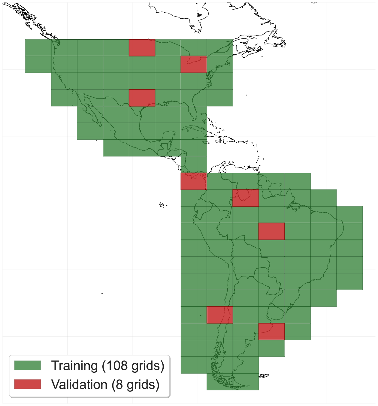
(a) Pretraining weather data coverage.

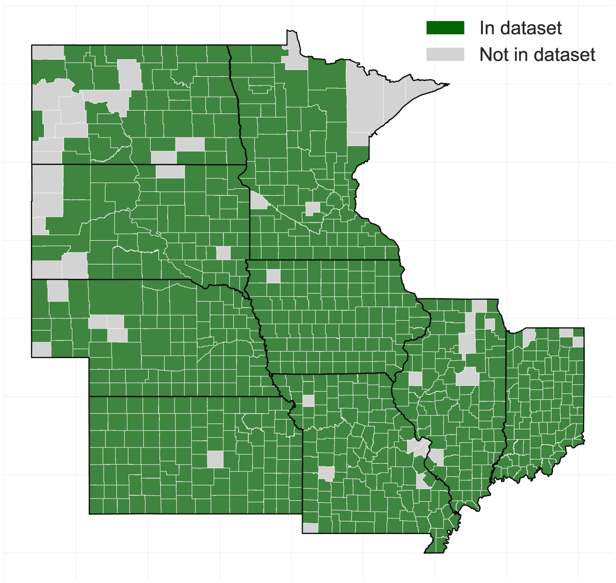
(b) Fine-tuning crop yield data coverage.

Figure 7: Spatial coverage of pretraining and fine-tuning datasets.

Pretraining Dataset Variables.

Here is a list of 31 weather measurements in the pretraining data. The first 28 measurements were downloaded from the NASA Power Project (NASA 2024) from 1984 to 2022. The last three were predicted using Teten’s equation (Vapor Pressure and Vapor Pressure Deficit) and FAO-Penman-Monteith equation (Reference Evapotranspiration). The data was downloaded for daily measurements and weekly mean was computed for each variable.

Measurement Name	Symbol	Unit
Temperature at 2 Meters	T2M	∘C
Temperature at 2 Meters Maximum	T2M_MAX	∘C
Temperature at 2 Meters Minimum	T2M_MIN	∘C
Wind Direction at 2 Meters	WD2M	Degrees
Wind Speed at 2 Meters	WS2M	m/s
Surface Pressure	PS	kPa
Specific Humidity at 2 Meters	QV2M	g/Kg
Precipitation Corrected	PRECTOTCORR	mm/day
All Sky Surface Shortwave Downward Irradiance	ALLSKY_SFC_SW_DWN	MJ/m2/day
Evapotranspiration Energy Flux	EVPTRNS	MJ/m2/day
Profile Soil Moisture (0 to 1)	GWETPROF	0 to 1
Snow Depth	SNODP	cm
Dew/Frost Point at 2 Meters	T2MDEW	∘C
Cloud Amount	CLOUD_AMT	0 to 1
Evaporation Land	EVLAND	kg/m2/s $\times 10^{6}$
Wet Bulb Temperature at 2 Meters	T2MWET	∘C
Land Snowcover Fraction	FRSNO	0 to 1
All Sky Surface Longwave Downward Irradiance	ALLSKY_SFC_LW_DWN	MJ/m2/day
All Sky Surface PAR Total	ALLSKY_SFC_PAR_TOT	MJ/m2/day
All Sky Surface Albedo	ALLSKY_SRF_ALB	0 to 1
Precipitable Water	PW	cm
Surface Roughness	Z0M	m
Surface Air Density	RHOA	kg/m3
Relative Humidity at 2 Meters	RH2M	0 to 1
Cooling Degree Days Above 18.3 C	CDD18_3	days
Heating Degree Days Below 18.3 C	HDD18_3	days
Total Column Ozone	TO3	Dobson units
Aerosol Optical Depth 55	AOD_55	0 to 1
Reference Evapotranspiration	ET0	mm/day
Vapor Pressure	VAP	kPa
Vapor Pressure Deficit	VAD	kPa

Table 12: Descriptions of the 31 weather measurements and their units.

References

- Basir et al. (2021) Basir, M. S.; Chowdhury, M.; Islam, M. N.; and Ashik-E-Rabbani, M. 2021. Artificial neural network model in predicting yield of mechanically transplanted rice from transplanting parameters in Bangladesh. Journal of Agriculture and Food Research, 5: 100186.
- Beddington (2010) Beddington, J. 2010. Food security: contributions from science to a new and greener revolution. Philosophical Transactions of the Royal Society B: Biological Sciences, 365(1537): 61–71.
- Brown (1951) Brown, O. L. I. 1951. The Clausius-Clapeyron equation. Journal of Chemical Education, 28(8): 428.
- Cao, Ma, and Zhang (2022) Cao, Z.; Ma, Y.; and Zhang, Z. 2022. Corn Yield Prediction based on Remotely Sensed Variables Using Variational Autoencoder and Multiple Instance Regression. arXiv:2211.13286.
- Chu and Yu (2020) Chu, Z.; and Yu, J. 2020. An end-to-end model for rice yield prediction using deep learning fusion. Computers and Electronics in Agriculture, 174: 105471.
- Dong et al. (2023) Dong, J.; Wu, H.; Zhang, H.; Zhang, L.; Wang, J.; and Long, M. 2023. SimMTM: A Simple Pre-Training Framework for Masked Time-Series Modeling. arXiv:2302.00861.
- Fan et al. (2021) Fan, J.; Bai, J.; Li, Z.; Ortiz-Bobea, A.; and Gomes, C. P. 2021. A GNN-RNN Approach for Harnessing Geospatial and Temporal Information: Application to Crop Yield Prediction. CoRR, abs/2111.08900.
- Ferraz et al. (2024) Ferraz, M. A. J.; Barboza, T. O. C.; Piza, M. R.; Von Pinho, R. G.; and dos Santos, A. F. 2024. Sorghum grain yield estimation based on multispectral images and neural network in tropical environments. Smart Agricultural Technology, 9: 100661.
- Franceschi, Dieuleveut, and Jaggi (2019) Franceschi, J.-Y.; Dieuleveut, A.; and Jaggi, M. 2019. Unsupervised scalable representation learning for multivariate time series. In Advances in Neural Information Processing Systems, volume 32.
- Gandhi, Petkar, and Armstrong (2016) Gandhi, N.; Petkar, O.; and Armstrong, L. J. 2016. Rice crop yield prediction using artificial neural networks. In 2016 IEEE Technological Innovations in ICT for Agriculture and Rural Development (TIAR), 105–110.
- Hendrycks and Gimpel (2023) Hendrycks, D.; and Gimpel, K. 2023. Gaussian Error Linear Units (GELUs). arXiv:1606.08415.
- Higgins et al. (2017) Higgins, I.; Matthey, L.; Pal, A.; Burgess, C.; Glorot, X.; Botvinick, M.; Mohamed, S.; and Lerchner, A. 2017. beta-VAE: Learning Basic Visual Concepts with a Constrained Variational Framework. In International Conference on Learning Representations.
- Khaki, Wang, and Archontoulis (2019) Khaki, S.; Wang, L.; and Archontoulis, S. V. 2019. A CNN-RNN Framework for Crop Yield Prediction. Frontiers in Plant Science, 10.
- Kingma et al. (2014) Kingma, D. P.; Mohamed, S.; Jimenez Rezende, D.; and Welling, M. 2014. Semi-supervised learning with deep generative models. Advances in neural information processing systems, 27.
- Kingma and Welling (2013) Kingma, D. P.; and Welling, M. 2013. Auto-encoding variational bayes. arXiv preprint arXiv:1312.6114.
- Kwok and Qi (2021) Kwok, P. H.; and Qi, Q. 2021. A Variational U-Net for Weather Forecasting. CoRR, abs/2111.03476.
- Lin et al. (2024) Lin, F.; Guillot, K.; Crawford, S.; Zhang, Y.; Yuan, X.; and Tzeng, N.-F. 2024. An Open and Large-Scale Dataset for Multi-Modal Climate Change-aware Crop Yield Predictions. In Proceedings of the 30th ACM SIGKDD Conference on Knowledge Discovery and Data Mining, 5375–5386. ACM.
- Lobell, Schlenker, and Costa-Roberts (2011) Lobell, D. B.; Schlenker, W.; and Costa-Roberts, J. 2011. Climate trends and global crop production since 1980. Science, 333(6042): 616–620.
- McFarland et al. (2020) McFarland, B. A.; AlKhalifah, N.; Bohn, M.; Bubert, J.; Buckler, E. S.; Ciampitti, I.; Edwards, J.; Ertl, D.; Gage, J. L.; Falcon, C. M.; Flint-Garcia, S.; Gore, M. A.; Graham, C.; Hirsch, C. N.; Holland, J. B.; Hood, E.; Hooker, D.; Jarquin, D.; Kaeppler, S. M.; Knoll, J.; Kruger, G.; Lauter, N.; Lee, E. C.; Lima, D. C.; Lorenz, A.; Lynch, J. P.; McKay, J.; Miller, N. D.; Moose, S. P.; Murray, S. C.; Nelson, R.; Poudyal, C.; Rocheford, T.; Rodriguez, O.; Romay, M. C.; Schnable, J. C.; Schnable, P. S.; Scully, B.; Sekhon, R.; Silverstein, K.; Singh, M.; Smith, M.; Spalding, E. P.; Springer, N.; Thelen, K.; Thomison, P.; Tuinstra, M.; Wallace, J.; Walls, R.; Wills, D.; Wisser, R. J.; Xu, W.; Yeh, C. T.; and de Leon, N. 2020. Maize genomes to fields (G2F): 2014-2017 field seasons: genotype, phenotype, climatic, soil, and inbred ear image datasets. BMC Research Notes, 13(1): 71.
- Murray-Tortarolo (2023) Murray-Tortarolo, G. 2023. A breviary of Earth’s climate changes using Stephan-Boltzmann law. Atmósfera, 37.
- NASA (2024) NASA. 2024. NASA Power API.
- National Drought Mitigation Center, NOAA, and USDA (2025) National Drought Mitigation Center; NOAA; and USDA. 2025. U.S. Drought Monitor. Accessed: 2025-07-31.
- Ndulue and Ranjan (2021) Ndulue, E.; and Ranjan, R. S. 2021. Performance of the FAO Penman-Monteith equation under limiting conditions and fourteen reference evapotranspiration models in southern Manitoba. Theoretical and Applied Climatology, 143(3): 1285–1298.
- O. Tetens (1930) O. Tetens. 1930. Über einige meteorologische Begriffe (On some meteorological terms). Z. Geophys., 6: 297–309.
- Oliveira et al. (2018) Oliveira, I.; Cunha, R. L. F.; Silva, B.; and Netto, M. A. S. 2018. A Scalable Machine Learning System for Pre-Season Agriculture Yield Forecast. arXiv:1806.09244.
- Palma et al. (2025) Palma, L.; Peraza, A.; Civantos, D.; Duarte, A.; Materia, S.; Ángel G. Muñoz; Peña-Izquierdo, J.; Romero, L.; Soret, A.; and Donat, M. G. 2025. Data-driven Seasonal Climate Predictions via Variational Inference and Transformers. arXiv:2503.20466.
- Razavi et al. (2024) Razavi, M. A.; Nejadhashemi, A. P.; Majidi, B.; Razavi, H. S.; Kpodo, J.; Eeswaran, R.; Ciampitti, I.; and Prasad, P. V. 2024. Enhancing crop yield prediction in Senegal using advanced machine learning techniques and synthetic data. Artificial Intelligence in Agriculture, 14: 99–114.
- Schauberger et al. (2017) Schauberger, B.; Archontoulis, S.; Arneth, A.; Balkovic, J.; Ciais, P.; Deryng, D.; Elliott, J.; Folberth, C.; Khabarov, N.; Müller, C.; Pugh, T. A. M.; Rolinski, S.; Schaphoff, S.; Schmid, E.; Wang, X.; Schlenker, W.; and Frieler, K. 2017. Consistent negative response of US crops to high temperatures in observations and crop models. Nature Communications, 8(1): 13931.
- Sun et al. (2019) Sun, J.; Di, L.; Sun, Z.; Shen, Y.; and Lai, Z. 2019. County-Level Soybean Yield Prediction Using Deep CNN-LSTM Model. Sensors, 19(20): 4363.
- U.S. Department of Agriculture, National Agricultural Statistics Service (2023) U.S. Department of Agriculture, National Agricultural Statistics Service. 2023. Quick Stats Database. https://quickstats.nass.usda.gov/. Accessed: 2025-07-08.
- USDA Farm Service Agency (2019) USDA Farm Service Agency. 2019. Report: Farmers Prevented from Planting Crops on 19 Million Acres. https://www.fsa.usda.gov/news-events/news/08-12-2019/report-farmers-prevented-planting-crops-19-million-acres. Accessed: 2025-07-22.
- USDA National Agricultural Statistics Service (2013) USDA National Agricultural Statistics Service. 2013. Crop Production 2012 Summary. https://www.nass.usda.gov/Newsroom/archive/2013/01˙11˙2013.php. Accessed: 2025-07-22.
- Vaswani et al. (2017) Vaswani, A.; Shazeer, N.; Parmar, N.; Uszkoreit, J.; Jones, L.; Gomez, A. N.; Kaiser, L.; and Polosukhin, I. 2017. Attention Is All You Need. arXiv:1706.03762.
- Wang et al. (2024) Wang, W.; Zhang, J.; Su, Q.; et al. 2024. Accurate initial field estimation for weather forecasting with a variational constrained neural network. npj Climate and Atmospheric Science, 7(1): 223.
- Williams and Pounds-Barnett (2024) Williams, B.; and Pounds-Barnett, G. 2024. As U.S. Farmers Respond to Crop Price Changes, Trends in Planted Acreage Emerge. Amber Waves.
- Woo et al. (2022) Woo, G.; Liu, C.; Sahoo, D.; Kumar, A.; and Hoi, S. 2022. CoST: Contrastive Learning of Disentangled Seasonal-Trend Representations for Time Series Forecasting. arXiv:2202.01575.
- Wu et al. (2023) Wu, H.; Xu, J.; Wang, J.; and Long, M. 2023. Patchtst: A general-purpose patch-based transformer for time series forecasting. In The Eleventh International Conference on Learning Representations.
- Wu et al. (2021) Wu, X.; Xiao, X.; Steiner, J.; Yang, Z.; Qin, Y.; and Wang, J. 2021. Spatiotemporal Changes of Winter Wheat Planted and Harvested Areas, Photosynthesis and Grain Production in the Contiguous United States from 2008–2018. Remote Sensing, 13(9).
- You et al. (2017) You, J.; Li, X.; Low, M.; Lobell, D.; and Ermon, S. 2017. Deep Gaussian process for crop yield prediction based on remote sensing data. arXiv preprint arXiv:1704.02720.
- Yue et al. (2022) Yue, Z.; Wang, Y.; Pang, J.; Zhang, F.; Yang, W.; Sun, L.; Li, J.; Wang, J.; and Zhang, Y. 2022. Ts2vec: Towards universal representation of time series. In Proceedings of the AAAI conference on artificial intelligence, volume 36, 8980–8988.
- Zerveas et al. (2021) Zerveas, G.; Jayaraman, S.; Patel, D.; Bhamidipaty, A.; and Eickhoff, C. 2021. A transformer-based framework for multivariate time series representation learning. In Proceedings of the 27th ACM SIGKDD conference on knowledge discovery & data mining, 2114–2124.