Witness the High-Dimensional Quantum Steering via Majorization Lattice
Abstract
Quantum steering enables one party to influence another remote quantum state by local measurement. While steering is fundamental to many quantum information tasks, the existing detection methods in the literature are mainly constrained to either specific measurement scenario or low-dimensional systems. In this work, we propose a majorization lattice framework for steering detection, which is capable of exploring the steering in arbitrary dimension and measurement setting. Steering inequalities for two-qubit states, high-dimensional Werner states and isotropic states are obtained, which set even stringent bars than what have reached yet. Notably, the known high-dimensional results turn out to be some kind of approximate limits of the new approach.
Introduction.—The concept of quantum steering can be traced back to the renowned debate on the completeness of quantum mechanics initiated by Einstein, Podolsky, and Rosen in 1935 [1], along with the subsequent responses from Schrödinger [2]. Quantum steering refers to the ability of one party (Alice) in a composite quantum system to influence the quantum state of another party (Bob) through local measurements. This phenomenon implies a distinct form of non-local correlations that are found exist between quantum entanglement and Bell non-locality [3, 4, 5].
Recently, a lot of efforts have been made to characterize and understand the quantum steering by means of local hidden state (LHS) models and steering inequalities. In seminal works [3, 6], Wiseman et al. established the steering thresholds for Werner states and isotropic states under projective measurements by constructing LHS models (c.f. also Ref. [7, 8]). Subsequent advances by Nguyen and Gühne determined the new thresholds for the restricted case of dichotomic measurements performed by Alice [9]. Very recently, people found the Wiseman et al.’s threshold condition remains valid for positive operator-valued measurements (POVMs) in qubit systems [10, 11], which challenges the presumed advantage of POVMs in quantum steering scenario. Moreover, similar to the Bell non-locality, quantum steering can be identified as well by the violation of some inequalities. This provides a practical way to detect the quantum steering in experiment. To this aim, various steering inequalities have been proposed, including the well-known Reid criteria [12], linear steering inequalities [13, 14], and steering inequalities based on various uncertainty relations [15, 16, 17, 18, 19, 20, 21, 22], among others (see reviews [23, 5, 24]). In recent years, high-dimensional quantum steering has garnered significant attention due to its enhanced robustness against noise and loss [25, 26, 27, 28, 29], while limited inequalities are established, merely applicable to qubit system or systems with specific measurement settings, such as mutually unbiased bases (MUBs).
Over the past few decades, majorization theory has found widespread applications across various aspects of quantum information science [30, 31, 32, 33, 34, 35, 36, 37, 38, 39, 40, 41]. Of particular significance is the majorization lattice [42, 43, 44, 45], which establishes an algebraic structure for the set of probability distributions, providing a framework that is naturally congruent with the probabilistic descriptions inherent to quantum theory. Recently, majorization theory has been applied to quantum steering [46, 22, 47] in lower-dimensional systems.
In this Letter, we present a systematic approach to the detection of quantum steering based on the probability majorization lattice. Notably, this method is applicable to any measurement setting and dimensional system, by which the quantum correlation information encoded in joint probabilities can then be fully extracted through tailored aggregation operations. This leads to lossless information extraction in contrast to conventional methods relying on functions of probability distributions, such as entropy and variance. To illustrate the efficacy of our approach, we derive steering inequalities for two-qubit systems, as well as for arbitrary-dimensional Werner states and isotropic states. In the MUBs scenario, our approach not only yields stronger steering inequalities compared to existing ones, but also indicates that previous high-dimensional steering inequalities can be systematically obtained in a series of approximations. In the following we present first the preliminary preparation for later use, then the derivation of central theorem, and representative examples confronting to the yet known results.
Preliminaries.—Majorization theory establishes a partial ordering relation between any two vectors with , which symbolizes , i.e. is majorized by , if and only if [48]
| (1) |
Here, the superscript denotes the components of and in decreasing order. For -dimensional probability vectors with components in decreasing order, we can define
| (2) |
The set , equipped with the majorization relation defined in Eq. 1, forms a lattice [42] (see [49] for thorough discussion). In mathematics, a lattice is defined as a quadruple, and a probability majorization lattice can be represented as , where for there is a unique infimum and a unique supremum . It is proved that the probability majorization lattice is a complete lattice and we have [43, 44, 45]
Lemma 1.
A probability majorization lattice is a complete lattice, meaning that for every subset , both the supremum and the infimum exist.
Probability majorization lattice provides an elegant formalism to establish state-independent uncertainty relation (UR). For any observables in a -dimensional Hilbert space 111There always exist an observable with non-degenerate and nonzero eigenvalues , satisfying . Therefore, we do not distinguish between a complete orthonormal basis and an observable derived from it and we use the two terms interchangeably., one can define the measurement distribution set as
| (3) |
Here, and are respectively the sets of probability vectors corresponding to the measurements and , such as with the set of density matrices for -dimensional Hilbert space ; denotes the binary operation that preserve the majorization relation, including direct sum, direct product, and vector sum, i.e. . In light of Lemma 1, a probability majorization lattice is a complete lattice and there exist the supremum for the subset 222 has different value for the different binary operation and is equal to for , respectively., which formulates the majorization-based state-independent UR:
| (4) |
where . Clearly, the statements above can be generalized to the scenario involving measurements. Note that the bound with binary operations has been extensively studied in references [35, 36, 37, 38, 39, 40, 41, 46].
Probability majorization lattice and quantum steering.—Assuming that Alice and Bob each possess one of the two subsystems of a bipartite state and measure on bases and respectively, in projective measurement, quantum theory predicts the joint probability
| (5) |
with projectors . Considering of all alternative measurements, a bipartite quantum state corresponds to the infinite set of joint probability , i.e.
| (6) |
If the LHS description does not exist, i.e. for certain measurements and , Alice can then demonstrably steer Bob’s state, hence exhibiting the quantum steering [3]. Here, , and denote the possible hidden variables, Alice’s measurement distribution and Bob’s local state, respectively.
In practical experiment, only finite number of measurement settings can be implemented. We define the set of the joint distributions of non-steerable states in -measurement scenario as follows:
| (7) |
Here, signifies the set of non-steerable states. Clearly, sets up a subset of the probability majorization lattice . Moreover, by Lemma 1, there exists a supremum over the all non-steerable states, from which the steerability condition follows:
Lemma 2.
Given the orthonormal complete base sets and for Hilbert spaces and , the violation of the following majorization inequality
| (8) |
signifies the steerability of quantum state .
Although Lemma 2 establishes a direct connection between quantum steering and probability majorization lattice, calculating the supremum presents an intractable challenge. It can be shown that in quantum steering scenario, the supremum can be replaced by majorization UR bound , thereby formulating an operational steering detection framework. To this end, we employ the concept of aggregating a probability distribution [52, 53, 54, 46]. Given probability vectors and , is refereed as an aggregation of if there is a partition of into disjoint sets such that , for . Vector can then be denoted as and we have the following theorem (proof shown in Supplemental Material Sec. I):
Theorem 1.
Given orthonormal complete base sets and for Hilbert spaces and , the violation of the following majorization inequality
| (9) |
signifies the steerability of quantum state (from Alice to Bob). Here, is majorization UR bound of for binary operations and denotes all aggregations of with partitions satisfying ; denotes the local transformations preserving the majorization UR bound , i.e. ; represents any local transformation of measurement Alice performs.
Theorem 1 provides a criterion for quantum steering that is applicable to arbitrary finite dimension and measurement settings. It offers a novel perspective that quantum correlation information embedded in the joint probability can be extracted through appropriate aggregation operations. Next, to exhibit the capacity of above theorem in steering detection, we first develop some steering inequalities from it and then apply the inequalities to three typical states, i.e. the qubit state, high-dimensional Werner state and isotropic state.
Witnessing quantum steering via majorization formalism.—For illustration, we herein focus on the binary operation and present some practical steering inequalities. Employing the Bloch representation, a bipartite state is expressed in the form of
| (10) |
Here, the coefficient matrix entries are , and with generators of Lie algebra. Let us consider the partition of with elements
| (11) | |||
| (12) |
where denotes modulo operation with offset and . It has been proved that the partition satisfies 333It is equivalent to the degenerate case of Lemma 1 in Ref. [33].. The partition results in an aggregation of with components
| (13) |
where is Bloch vectors of projectors. Based upon Theorem 1, we obtain the following majorization steering inequality:
| (14) |
which yields a family of aggregation steering inequalities
| (15) |
Here, denotes the largest -th component of a vector and with . Similar to qubit situation [13], we define quantity as the steering parameter for measurement settings in arbitrary dimensional Hilbert space. The calculation of is a typical combinatorial optimization problem (COP) (see Supplemental Material Sec. II for details). Nevertheless, there indeed exists approximate analytic upper bounds for in the MUBs (see proof in Supplemental Material Sec. III):
| (16) |
where with the floor function and . Next, we formulate quantum steering inequalities in two-qubit systems, arbitrary-dimensional Werner states and isotropic states, with detailed calculations given in Supplemental Material Sec. IV.
Two qubits system. Given spin observables and with Pauli matrices vector , we have the aggregated joint probability for two qubit system
| (17) |
Here, is the singular value vector of ; denotes Hadamard product. Considering 2-qubit Werner state with and setting , we have and
| (18) |
which yields a steering threshold for 2-qubit Werner state: . Notably, this result is equivalent to the linear steering inequality established by Saunders et al. [13]. Furthermore, when measurements are conducted over the entire hemisphere of the Bloch sphere, there exists a limit of , which leads to a threshold of . This confirms the recent finding in Refs. [10, 11] from a reversed perspective.
Isotropic state and Werner state in d dimension. Without loss of generality, one can set and with , where are dimensional real vectors. For isotropic states and Werner states, we have the aggregated joint probability
| (19) | ||||
| (20) |
and
| (21) |
Here, and are noise parameters for the isotropic and Werner state, respectively. By Eq. 15, we obtain the steering threshold for isotropic and Werner states, respectively
| (22) | ||||
| (23) |
For the case of two measurement settings, we obtain with representing the maximal overlap of the two bases. The steering threshold is then , which implies that the results in Refs. [56, 27, 57] are the special cases corresponding to MUBs pair.
| Bounds | ||
|---|---|---|
Utilizing the approximate upper bounds derived in Eq. 16, we obtain approximate steering thresholds for isotropic states and Werner states, as summarized in Table 1. These bounds provide an excellent approximation for isotropic state steering scenario involving MUBs, which significantly simplifies the analysis of steering in high-dimensional system. Note, the thresholds in Refs. [25, 29, 20] are compatible with the approximations of and , respectively, which indicates that those previous results are not optimal ones for isotropic state. As illustrated in Fig. 1, we compute the optimal steering thresholds for various isotropic states with MUBs dimensions, from to for illustration, and compare these thresholds with those from , as well as the critical values from LHS model [7, 3, 8].
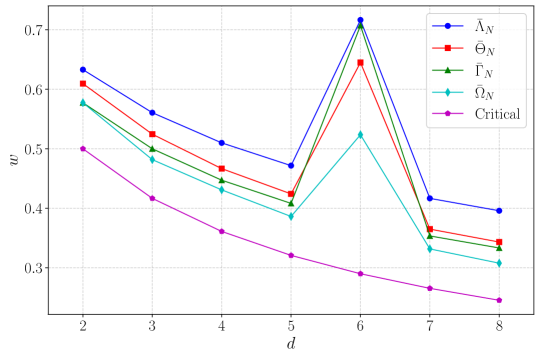
It is noteworthy that for , the steering threshold of Werner states in Table 1 exceeds , i.e. , which indicates that MUBs fail to witness the steerability of Werner states in high dimensions. Numerical results of further show that for MUBs at dimensions , and it possibly holds for even higher dimensions. These findings highlight an intriguing fact that while MUBs effectively capture the steerability of isotropic states, they are inadequate for witnessing the steerability of Werner states in high dimensions.
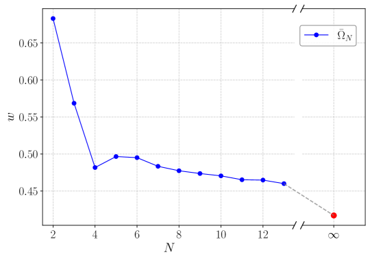
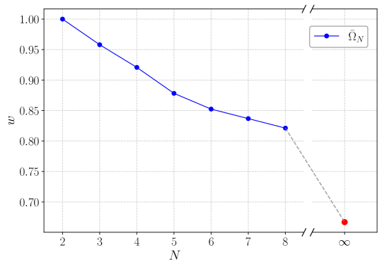
Notice that the new approach enables the investigation of optimal measurement settings for quantum steering. Consequently, we are tasked with addressing the optimization problem
| min | (24) | |||
| s.t. |
In Fig. 2, we examine the optimal settings for qutrit isotropic and Werner states using the Cross-Entropy Method (CEM) [58, 59], a powerful technique for solving complex continuous optimization problems and machine learning tasks. As shown in Figs. 2a and 2b, we compute the steering thresholds for qutrit isotropic states in to measurement settings and for qutrit Werner states in to measurement settings. Our results indicate that MUBs remain optimal for in isotropic scenario. However, to certify the steerability of qutrit Werner states, optimal measurement settings must be non-MUBs. Lower thresholds are achieved as the number of measurement settings increases. We conjecture that the critical values and can be attained in the limit as for both qutrit isotropic and Werner states, respectively, similar to the scenario in two-qubit Werner states.
Conclusions.—In this Letter, we have established a connection between quantum steering and the probability majorization lattice, leading to a novel framework for detecting quantum steering. This framework is applicable to arbitrary finite dimensions and measurement settings. By introducing the concept of aggregating probability distributions, we have formulated a family of aggregation-based steering inequalities and applied them to 2-qubit systems as well as arbitrary-dimensional Werner and isotropic states.
From the perspective of information theory, our approach facilitates the extraction of quantum correlation information embedded in the joint probability without loss, utilizing appropriate aggregation operations that differ from those based on entropies and variances. In the context of mutually unbiased bases (MUBs), our approach not only reproduces known steering inequalities as approximate cases but also provides improved thresholds and new insights into the optimal measurement settings for detecting quantum steerability.
For high-dimensional Werner states, we demonstrate that MUBs fail to witness steerability, underscoring the necessity for non-MUB measurements to detect the quantum steerability of generic states. We investigate the optimal -measurement settings for qutrit isotropic and Werner states using the Cross-Entropy Method (CEM), revealing that MUBs remain optimal for in the isotropic scenario, while non-MUBs are required for qutrit Werner states.
High-dimensional quantum systems have garnered significant attentions in quantum information processing due to their enhanced resilience to noise, reduced susceptibility to loss, and greater information capacity. These advantages render them particularly valuable for applications in quantum communication [60, 61, 62], quantum cryptography [63], and superdense coding [64]. Hopefully, the majorization-based framework for quantum steering may enlighten our understanding of quantum correlation and facilitate practical applications across these areas.
Acknowledgements.—This work was supported in part by the National Natural Science Foundation of China (NSFC) under the Grants 12475087, 12235008, the Fundamental Research Funds for Central Universities, and China Postdoctoral Science Foundation funded project No. 2024M753174.
References
- Einstein et al. [1935] A. Einstein, B. Podolsky, and N. Rosen, Can quantum-mechanical description of physical reality be considered complete?, Phys. Rev. 47, 777 (1935).
- Schrödinger [1935] E. Schrödinger, Discussion of probability relations between separated systems, Math. Proc. Cambridge Philos. Soc. 31, 555 (1935).
- Wiseman et al. [2007] H. M. Wiseman, S. J. Jones, and A. C. Doherty, Steering, entanglement, nonlocality, and the Einstein-Podolsky-Rosen paradox, Phys. Rev. Lett. 98, 140402 (2007).
- Quintino et al. [2015] M. T. Quintino, T. Vértesi, D. Cavalcanti, R. Augusiak, M. Demianowicz, A. Acín, and N. Brunner, Inequivalence of entanglement, steering, and Bell nonlocality for general measurements, Phys. Rev. A 92, 032107 (2015).
- Uola et al. [2020] R. Uola, A. C. S. Costa, H. C. Nguyen, and O. Gühne, Quantum steering, Rev. Mod. Phys. 92, 015001 (2020).
- Jones et al. [2007] S. J. Jones, H. M. Wiseman, and A. C. Doherty, Entanglement, Einstein-Podolsky-Rosen correlations, bell nonlocality, and steering, Phys. Rev. A 76, 052116 (2007).
- Werner [1989] R. F. Werner, Quantum states with Einstein-Podolsky-Rosen correlations admitting a hidden-variable model, Phys. Rev. A 40, 4277 (1989).
- Almeida et al. [2007] M. L. Almeida, S. Pironio, J. Barrett, G. Toth, and A. Acin, Noise robustness of the nonlocality of entangled quantum states, Phys. Rev. Lett. 99, 040403 (2007).
- Nguyen and Guhne [2020] H. C. Nguyen and O. Guhne, Some quantum measurements with three outcomes can reveal nonclassicality where all two-outcome measurements fail to do so, Phys. Rev. Lett. 125, 230402 (2020).
- Zhang and Chitambar [2024] Y. Zhang and E. Chitambar, Exact steering bound for two-qubit werner states, Phys. Rev. Lett. 132, 250201 (2024).
- Renner [2024] M. J. Renner, Compatibility of generalized noisy qubit measurements, Phys. Rev. Lett. 132, 250202 (2024).
- Reid [1989] M. D. Reid, Demonstration of the Einstein-Podolsky-Rosen paradox using nondegenerate parametric amplification, Phys. Rev. A 40, 913 (1989).
- Saunders et al. [2010] D. J. Saunders, S. J. Jones, H. M. Wiseman, and G. J. Pryde, Experimental EPR-steering using Bell-local states, Nat. Phys. 6, 845 (2010).
- Zheng et al. [2017] Y.-L. Zheng, Y.-Z. Zhen, W.-F. Cao, L. Li, Z.-B. Chen, N.-L. Liu, and K. Chen, Optimized detection of steering via linear criteria for arbitrary-dimensional states, Phys. Rev. A 95, 032128 (2017).
- Walborn et al. [2011] S. P. Walborn, A. Salles, R. M. Gomes, F. Toscano, and P. H. S. Ribeiro, Revealing hidden Einstein-Podolsky-Rosen nonlocality, Phys. Rev. Lett. 106, 130402 (2011).
- Schneeloch et al. [2013] J. Schneeloch, C. J. Broadbent, S. P. Walborn, E. G. Cavalcanti, and J. C. Howell, Einstein-Podolsky-Rosen steering inequalities from entropic uncertainty relations, Phys. Rev. A 87, 062103 (2013).
- Zhen et al. [2016] Y.-Z. Zhen, Y.-L. Zheng, W.-F. Cao, L. Li, Z.-B. Chen, N.-L. Liu, and K. Chen, Certifying Einstein-Podolsky-Rosen steering via the local uncertainty principle, Phys. Rev. A 93, 012108 (2016).
- Maity et al. [2017] A. G. Maity, S. Datta, and A. S. Majumdar, Tighter Einstein-Podolsky-Rosen steering inequality based on the sum-uncertainty relation, Phys. Rev. A 96, 052326 (2017).
- Riccardi et al. [2018] A. Riccardi, C. Macchiavello, and L. Maccone, Multipartite steering inequalities based on entropic uncertainty relations, Phys. Rev. A 97, 052307 (2018).
- Costa et al. [2018] A. C. S. Costa, R. Uola, and O. Gühne, Steering criteria from general entropic uncertainty relations, Phys. Rev. A 98, 050104 (2018).
- Kriváchy et al. [2018] T. Kriváchy, F. Fröwis, and N. Brunner, Tight steering inequalities from generalized entropic uncertainty relations, Phys. Rev. A 98, 062111 (2018).
- Li and Qiao [2021] J.-L. Li and C.-F. Qiao, Characterizing quantum nonlocalities per uncertainty relation, Quantum Inf. Process. 20, 109 (2021).
- Cavalcanti and Skrzypczyk [2017] D. Cavalcanti and P. Skrzypczyk, Quantum steering: a review with focus on semidefinite programming, Rep. Prog. Phys. 80, 024001 (2017).
- Xiang et al. [2022] Y. Xiang, S. Cheng, Q. Gong, Z. Ficek, and Q. He, Quantum steering: Practical challenges and future directions, PRX Quantum 3, 030102 (2022).
- Skrzypczyk and Cavalcanti [2015] P. Skrzypczyk and D. Cavalcanti, Loss-tolerant einstein-podolsky-rosen steering for arbitrary-dimensional states: Joint measurability and unbounded violations under losses, Phys. Rev. A 92, 022354 (2015).
- Skrzypczyk and Cavalcanti [2018] P. Skrzypczyk and D. Cavalcanti, Maximal randomness generation from steering inequality violations using qudits, Phys. Rev. Lett. 120, 260401 (2018).
- Zeng et al. [2018] Q. Zeng, B. Wang, P. Li, and X. Zhang, Experimental high-dimensional einstein-podolsky-rosen steering, Phys. Rev. Lett. 120, 030401 (2018).
- Srivastav et al. [2022] V. Srivastav, N. H. Valencia, W. McCutcheon, S. Leedumrongwatthanakun, S. Designolle, R. Uola, N. Brunner, and M. Malik, Quick quantum steering: Overcoming loss and noise with qudits, Phys. Rev. X 12, 041023 (2022).
- Qu et al. [2022] R. Qu, Y. Wang, M. An, F. Wang, Q. Quan, H. Li, H. Gao, F. Li, and P. Zhang, Retrieving high-dimensional quantum steering from a noisy environment with n measurement settings, Phys. Rev. Lett. 128, 240402 (2022).
- Nielsen [1999] M. A. Nielsen, Conditions for a class of entanglement transformations, Phys. Rev. Lett. 83, 436 (1999).
- Nielsen and Vidal [2001] M. A. Nielsen and G. Vidal, Majorization and the interconversion of bipartite states, Quantum Inf. Comput. 1, 76 (2001).
- Nielsen and Kempe [2001] M. A. Nielsen and J. Kempe, Separable states are more disordered globally than locally, Phys. Rev. Lett. 86, 5184 (2001).
- Gühne and Lewenstein [2004] O. Gühne and M. Lewenstein, Entropic uncertainty relations and entanglement, Phys. Rev. A 70, 022316 (2004).
- Partovi [2012] M. H. Partovi, Entanglement detection using majorization uncertainty bounds, Phys. Rev. A 86, 022309 (2012).
- Partovi [2011] M. H. Partovi, Majorization formulation of uncertainty in quantum mechanics, Phys. Rev. A 84, 052117 (2011).
- Friedland et al. [2013] S. Friedland, V. Gheorghiu, and G. Gour, Universal uncertainty relations, Phys. Rev. Lett. 111, 230401 (2013).
- Puchała et al. [2013] Z. Puchała, Ł. Rudnicki, and K. Życzkowski, Majorization entropic uncertainty relations, J. Phys. A: Math. Theor. 46, 272002 (2013).
- Rudnicki et al. [2014] L. Rudnicki, Z. Puchała, and K. Zyczkowski, Strong majorization entropic uncertainty relations, Phys. Rev. A 89, 052115 (2014).
- Li et al. [2016] T. Li, Y. Xiao, T. Ma, S. M. Fei, N. Jing, X. Li-Jost, and Z. X. Wang, Optimal universal uncertainty relations, Sci Rep 6, 35735 (2016).
- Li and Qiao [2019] J.-L. Li and C.-F. Qiao, The optimal uncertainty relation, Ann Phys 531, 1900143 (2019).
- Puchała et al. [2018] Z. Puchała, Ł. Rudnicki, A. Krawiec, and K. Życzkowski, Majorization uncertainty relations for mixed quantum states, J. Phys. A: Math. Theor. 51, 175306 (2018).
- Cicalese and Vaccaro [2002] F. Cicalese and U. Vaccaro, Supermodularity and subadditivity properties of the entropy on the majorization lattice, IEEE Trans. Inf Theory 48, 933 (2002).
- Alberti and Uhlmann [1982] P. M. Alberti and A. Uhlmann, Stochasticity and partial order (Springer Dordrecht, 1982).
- Bapat [1991] R. B. Bapat, Majorization and singular values. iii, Linear Algebra Appl 145, 59 (1991).
- Bondar [1994] J. V. Bondar, Comments on and complements to inequalities: Theory of majorization and its applications: by albert w. marshall and ingram olkin, Linear Algebra Appl 199, 115 (1994).
- Li and Qiao [2020] J.-L. Li and C.-F. Qiao, An optimal measurement strategy to beat the quantum uncertainty in correlated system, Adv. Quantum Technol. 3, 2000039 (2020).
- Zhu et al. [2023] G. Zhu, A. Liu, L. Xiao, K. Wang, D. Qu, J. Li, C. Qiao, and P. Xue, Experimental investigation of conditional majorization uncertainty relations in the presence of quantum memory, Phys. Rev. A 108, L050202 (2023).
- Marshall et al. [1979] A. W. Marshall, I. Olkin, and B. C. Arnold, Inequalities: theory of majorization and its applications (Springer, 1979).
- Davey and Priestley [2002] B. A. Davey and H. A. Priestley, Introduction to Lattices and Order, 2nd ed. (Cambridge University Press, Cambridge, 2002).
- Note [1] There always exist an observable with non-degenerate and nonzero eigenvalues , satisfying . Therefore, we do not distinguish between a complete orthonormal basis and an observable derived from it and we use the two terms interchangeably.
- Note [2] has different value for the different binary operation and is equal to for , respectively.
- Vidyasagar [2012] M. Vidyasagar, A metric between probability distributions on finite sets of different cardinalities and applications to order reduction, IEEE Transactions on Automatic Control 57, 2464 (2012).
- Cicalese et al. [2016] F. Cicalese, L. Gargano, and U. Vaccaro, Approximating probability distributions with short vectors, via information theoretic distance measures (2016).
- Cicalese et al. [2019] F. Cicalese, L. Gargano, and U. Vaccaro, Minimum-entropy couplings and their applications, IEEE Trans. Inf Theory 65, 3436 (2019).
- Note [3] It is equivalent to the degenerate case of Lemma 1 in Ref. [33].
- Li et al. [2015] C. M. Li, K. Chen, Y. N. Chen, Q. Zhang, Y. A. Chen, and J. W. Pan, Genuine high-order Einstein-Podolsky-Rosen steering, Phys. Rev. Lett. 115, 010402 (2015).
- Guo et al. [2019] Y. Guo, S. Cheng, X. Hu, B. H. Liu, E. M. Huang, Y. F. Huang, C. F. Li, G. C. Guo, and E. G. Cavalcanti, Experimental measurement-device-independent quantum steering and randomness generation beyond qubits, Phys. Rev. Lett. 123, 170402 (2019).
- de Boer et al. [2005] P.-T. de Boer, D. P. Kroese, S. Mannor, and R. Y. Rubinstein, A tutorial on the cross-entropy method, Annals of Operations Research 134, 19–67 (2005).
- Botev et al. [2013] Z. I. Botev, D. P. Kroese, R. Y. Rubinstein, and P. L’Ecuyer, The cross-entropy method for optimization, in Handbook of Statistics - Machine Learning: Theory and Applications, Handbook of Statistics (2013) p. 35–59.
- Branciard et al. [2012] C. Branciard, E. G. Cavalcanti, S. P. Walborn, V. Scarani, and H. M. Wiseman, One-sided device-independent quantum key distribution: Security, feasibility, and the connection with steering, Phys. Rev. A 85, 010301 (2012).
- Islam et al. [2017] N. T. Islam, C. C. W. Lim, C. Cahall, J. Kim, and D. J. Gauthier, Provably secure and high-rate quantum key distribution with time-bin qudits, Sci Adv 3, e1701491 (2017).
- Cozzolino et al. [2019] D. Cozzolino, B. Da Lio, D. Bacco, and L. K. Oxenløwe, High‐dimensional quantum communication: Benefits, progress, and future challenges, Adv. Quantum Technol. 2, 10.1002/qute.201900038 (2019).
- Gröblacher et al. [2006] S. Gröblacher, T. Jennewein, A. Vaziri, G. Weihs, and A. Zeilinger, Experimental quantum cryptography with qutrits, New J. Phys. 8, 75–75 (2006).
- Hu et al. [2018] X. M. Hu, Y. Guo, B. H. Liu, Y. F. Huang, C. F. Li, and G. C. Guo, Beating the channel capacity limit for superdense coding with entangled ququarts, Sci Adv 4, eaat9304 (2018).
- Horn and Johnson [2013] R. A. Horn and C. R. Johnson, Matrix analysis (Cambridge University Press, 2013) Theorem 7.3.3.
- Kittaneh [1997] F. Kittaneh, Norm inequalities for certain operator sums, Journal of Functional Analysis 143, 337 (1997).
- Schaffner [2007] C. Schaffner, Cryptography in the Bounded-Quantum-Storage Model, Thesis (2007).
- Tomamichel et al. [2013] M. Tomamichel, S. Fehr, J. Kaniewski, and S. Wehner, A monogamy-of-entanglement game with applications to device-independent quantum cryptography, New J. Phys. 15, 10.1088/1367-2630/15/10/103002 (2013).
- Horodecki and Horodecki [1999] M. Horodecki and P. Horodecki, Reduction criterion of separability and limits for a class of distillation protocols, Phys. Rev. A 59, 4206 (1999).
- Pfeifer [2003] W. Pfeifer, The Lie algebras su(N) (Birkhäuser, Basel, 2003).
Witness the High-Dimensional Quantum Steering via Majorization Lattice
Supplemental Material
I The proof of Theorem 1
Given , we say that is an aggregation of if there is a partition of into disjoint sets such that , for , simply denoted as with . The aggregations of a probability distribution contain the less uncertainty than the original one, and there is the following result [53]:
Lemma 3.
Given and any aggregation of , we have .
Let and be any two probability distributions. We construct a new probability distribution with marginal probabilities and . Assuming that is a partition of , we have the aggregation of with . In fact, the partitions , or equivalently the aggregations , that we are interested in are those that satisfy
| (25) |
Obviously, an identity belongs to this, i.e. , because and are aggregations of . Note that Eq. 25 is a generalization of Lemma 1 in Ref. [33]. Specifically, every iteration of the degenerate case in Lemma 1 of Ref. [33] corresponds to a partition with
| (26) | |||
| (27) |
The non-steerable sates (by Alice) satisfy the mixed description of the joint probability for any two measurements [3]
| (28) |
Here, are the probability response function and local state of Alice and Bob, respectively; is a normalized distribution involving the hidden variable and . For convenience, Eq. 28 can be in form of
| (29) |
with and . If is a partition of satisfying , then we have for non-steerable states
| (30) |
Since the binary operation preserves the majorization relation, the majorization-based steering inequality is claimed
| (31) |
Here, is the majorization UR bound of measurement bases . In light of the local hidden state model of non-steerable states, Bob’s measurements satisfy the majorization UR, while Alice’s do not have any constraints. Thus, this result can be optimized by leveraging the symmetries inherent in the majorization UR bound and we have
| (32) |
Here, denotes the local transformations preserving the majorization UR bound , i.e. ; denotes any local transformation of Alice’s measurements.
II of measurement bases
Given orthonormal and complete bases for , we define the index set and the subsets , where denotes the index set of the -th basis. Assuming we choose base vectors from the bases, with each basis selecting vectors, we can define the projectors , as follows:
| (33) | |||
| (34) | |||
| (35) |
With the help of these notations, for measurements is defined as [36, 40]
| (36) | ||||
| (37) |
Here denotes the -th largest component of a vector and denotes the operator norm, i.e. the largest singular value of the operator. Especially, if we have (the possible maximal value), which occurs if and , . The solution of is a typical combinatorial optimization problem (COP), which has a discrete set of feasible solutions with a size of . Then, we provides a few equivalent expressions of for measurements.
Bloch representation. Let be Bloch vectors of . Under Bloch representation, the projectors are in form of . Thus, we have
| (38) | ||||
| (39) | ||||
| (40) |
Here, . Clearly, a concise expression can be derived for the qubit system
| (41) |
Transition matrix representation. Here, we formulate via the transition matrices between measurement bases.
| (42) | ||||
| (43) | ||||
| (44) | ||||
| (45) |
Here, we have employed the property of operator norm in the last line and denotes the largest eigenvalue of the operator and . The operator is defined as
| (46) |
where is the identity matrix of size and is the submatrix of entries that lie in the rows of the transition matrix indexed by and the columns indexed by , i.e. .
Two measurement bases scenario. When the involved measurement bases are two orthonormal complete bases, i.e. , we have
| (47) |
In light of Theorem 7.3.3 in Ref. [65], we have , and thus
| (48) | |||
| (49) |
Here, denotes the maximal singular value and for . If or , we have or . So, the first three terms have the analytical expressions
| (50) | |||
| (51) |
Mutual unbiased bases. For a pair of mutual unbiased bases (MUBs), the transition matrix between them is a discrete Fourier transformation (DFT) matrix, i.e.
| (58) |
where is a -th root of unity. For a pair of -dimensional MUBs, we conjecture the following expression.
Conjecture.
| (59) |
Here, and denotes the floor and the ceiling functions, respectively.
III The approximate upper bounds of
Here, we present some approximate upper bounds of for measurement bases.
III.1 Relaxation of optimization problem and the upper bound
is defined as the following optimization problem
| (60) |
Let and be the eigenvalues of . In order to find an upper bound of , we consider the following relaxation of the optimization problem of
| s.t. | ||||
| (61) | ||||
where, . Obviously, the solution of the optimization problem Eq. 61 offers an upper bound of . In particular, if we only consider the first two constraints, i.e. and , then we have the following upper bound
| (62) |
with definition .
Proof.
The solution of is equivalent to the following optimization problem
| s.t. | (63) | |||
| (64) | ||||
When maximize, other variables should be equal, namely setting , and with . Substituting these into the constraints, we obtain the following quadratic equation
| (65) |
So, we have . By reductio ad absurdum, it can be shown that cannot be larger than this value. If there exists , then we have and , where we have used the Cauchy-Schwarz inequality. Finally, we reach a contradiction . This completes the proof. ∎
III.2 The approximate upper bounds based on the operator norm inequalities
Lemma 4.
If are normalized state vectors acting on an arbitrary -dimensional Hilbert space , then we have the following inequalities
| (66) | |||
| (67) |
III.3 The upper bounds , and of for MUBs.
Assuming that are -dimensional MUBs, then we have
| (73) |
Substituting Eq. 73 into , we have
| (74) | ||||
| (75) | ||||
| (76) | ||||
| (77) | ||||
| (78) | ||||
| (79) |
where with the floor function . Substituting this into , we have
| (80) | ||||
| (81) |
Substituting Eq. 73 into and respectively, we have
| (82) | ||||
| (83) |
Finally, we formulate three analytical upper bounds of for MUBs as follows
| (84) |
It is worth noting that though is tighter than for MUBs scenario, provides a tighter upper bound than for general measurement bases. For a complete set of MUBs, provides a tighter upper bound than and as shown in Table 2.
| 2 | 0.8536/0.8536/0.8536/0.8660 | 0.7887/0.7887/0.8047/0.8165 | 0.75/0.75/0.7803/0.7906 | 0.7236/0.7236/0.7657/0.7746 | 0.7041/0.7041/0.7559/0.7638 | 0.6890/0.6890/0.7489/0.7560 |
| 3 | 0.7887/0.8047/0.7887/0.8165 | 0.7124/0.7182/0.7182/0.7454 | 0.6667/0.6667/0.6830/0.7071 | 0.6315/0.6315/0.6619/0.6831 | 0.6030/0.6055/0.6478/0.6667 | 0.5846/0.5853/0.6377/0.6547 |
| 4 | 0.6545/0.6830/0.6667/0.7071 | 0.625/0.625/0.625/0.6614 | 0.5693/0.5854/0.6/0.6325 | -/-/- | 0.5276/0.5335/0.5714/0.5976 | |
| 5 | 0.5732/0.6/0.5854/0.6325 | 0.5343/0.5578/0.5578/0.6 | -/-/- | 0.4960/0.5024/0.5262/0.5606 | ||
| 6 | 0.5090/0.5393/0.5266/0.5774 | -/-/- | 0.4743/0.4816/0.4928/0.5345 | |||
| 7 | -/-/- | 0.4587/0.4668/0.4668/0.5151 | ||||
| 8 | 0.4272/0.4557/0.4460/0.5 | |||||
IV Majorization steering inequalities in some scenarios
Here, we present the majorization steering inequalities for 2-qubit states, isotropic states and Werner states. We consider the partition of with elements
| (85) |
Here denotes modulo operation with offset . The partition results in an aggregation of with
| (86) |
where is Bloch vector of projectors and is correlation matrix of . Given observables and , Theorem 1 in the main text yields the following steering inequality:
| (87) |
where the joint probability is
| (88) | ||||
| (89) |
Here, () are the Bloch vectors of projectors () of (); () denotes Bloch vector of projectors of (). Immediately, a based-aggregation steering inequality yields
| (90) |
Here denotes the -th largest component of a vector and with . We have defined the quantity as the steering parameter for measurement settings in arbitrary dimensional Hilbert space.
IV.1 Two qubits system
For qubit dichotomy measurements and with , we have and and similarly for , which results in
| (91) |
and with .
Now, we consider the local transformation with and , which preserves the majorization UR bound, obviously. Simultaneously, we set the local transformation with and , whereupon we have
| (92) | ||||
| (93) |
Let the local transformations and conduct the singular value decomposition of , i.e. . Then we have
| (94) |
Here, is singular value vector of correlation matrix of quantum state and denotes Hadamard product.
Considering that 2-qubit Werner state with and setting , then we have and the violation of the following inequality signifies the steerability of 2-qubit Werner states:
| (95) |
We note that Saunders et al. formulated the following linear steering inequality [13]
| (96) |
where and . denotes the largest eigenvalue of . It is evident that our approach, along with Saunders et al.’s inequality Eq. 96, is equivalent for 2-qubit Werner states due to (readily verified by employing the Bloch representation given in Eq. 41 of ).
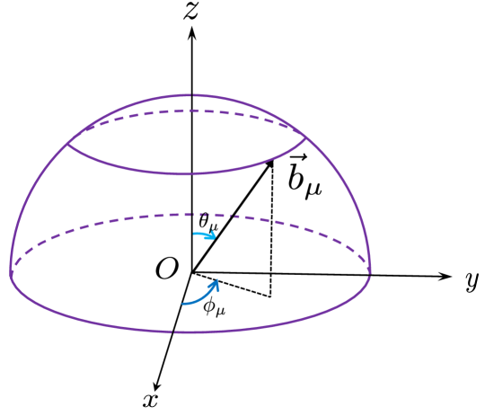
Infinite measurement settings scenario. Eq. 95 offers an elegant method to discuss the steerability involving with the infinite measurement settings, which corresponds to calculate the limitation when measurements are performed for the entire hemisphere as depicted in Fig. 3. In this case, the limitation can be calculated as follows:
| (97) | ||||
| (98) |
where we have set . Under the spherical coordinate, it is readily to see that with and . Similarly, we obtain and . Thus, we have , which achieves the critical value of steerability for 2-qubit Werner states. Especially, when the measurements are constrained to the half-plane, i.e. , we have and the threshold of steerability.
IV.2 The isotropic states and Werner states
Bloch representation and description of quantum states. We now focus on the arbitrary dimensional Werner and isotropic states. The isotropic states are defined as [69]
| (99) |
Here, is the fidelity of the state with respect to the maximally entangled state , i.e. with . An alternative form of the isotropic states is given by the maximally entangled states with white noise, i.e. with . The Werner states are defined as [3]
| (100) |
where is the swap operator defined as and . It is straightforward to convert Eqs. 99 and 100 into their Bloch representations
| (101) | ||||
| (102) |
Without loss of generality, one can set the first generators are antisymmetric and the last generators are symmetric, i.e. for and for [70]. Then the correlation matrices of the isotropic states and Werner states are given by with and , respectively.
Measurement settings. Without loss of generality, one can set and with , where are dimensional real vectors. After the aggregation with partition Eq. 85, the joint probability reads as
| (103) |
The correlation matrix of Werner state is a constant matrix and hence the optimal local transformations and should be identity operation, which leads to the joint probability
| (104) |
Setting and employing due to the orthonormality , we have
| (105) | ||||
| (106) |
Next, we consider the isotropic states whose joint probability reads as
| (107) |
Setting and the local transformations with , we have
| (108) | ||||
| (109) | ||||
| (110) |
Majorization steering inequalities. In light of above results, we have
| (111) |
Therefore, the majorization steering inequalities for Werner and isotropic states are given by
| (112) |
Obviously, we recover the qubit result for as expected.