Entanglement negativity in free fermions: twisted characteristic polynomial,
universal bounds, and area laws

Abstract

We present a general and simple formula for computing the entanglement negativity in free fermions. Our formula allows for deriving several universal bounds on negativity and its rate of change in dynamics. The bound on negativity directly relates the clustering property of correlations in free-fermion states to the entanglement area law, and provides the optimal condition for the area law in mixed free fermion states with long-range correlations. In addition, we establish an area-law bound on entanglement generation in open systems, analogous to previously known results for entanglement entropy in unitary dynamics. Our work provides new analytical insights into fermionic mixed-state entanglement.

Introduction.— Understanding quantum entanglement in mixed states is a central challenge in modern physics and quantum information science. This is essential for deciphering the quantum features in realistic systems at finite temperatures or coupled to an environment [1, 2, 3, 4]. Entanglement negativity has emerged as an indispensable tool for this challenge, providing a computable measure that successfully captures quantum correlations beyond the scope of entanglement entropy for bipartite pure states [5]. Its application to both (multipartite) closed and open quantum many-body systems has yielded fruitful insights across various contexts, including critical phenomena [6, 7, 8], nonequilibrium dynamics [9, 10], and topological phases [11, 12]. In particular, its computability has served as a powerful analytical tool for deriving rigorous results about mixed-state entanglement in bosonic and spin systems [13, 14, 15, 10, 8, 16].

However, extending the notion of negativity to fermionic systems turns out to be highly nontrivial, as the entanglement structure differs fundamentally from that of bosons due to the anticommuting nature of fermionic operators and the intrinsic superselection rules [17, 18, 19, 20, 21, 22]. These properties necessitate a different definition of negativity to correctly capture fermionic entanglement. A breakthrough was made in Ref. [23], which reinterprets the partial transpose as a partial time-reversal transformation. This allows for a quantum-information-theoretically consistent extension to fermionic systems [23, 24]. The transposed density matrix can be restored to be Hermitian by the fermion parity operator [25]. Nevertheless, both analytical and practical computations of negativity turn out to be extremely involved even for free fermions. It thus remains elusive to rigorously analyze universal properties of fermionic mixed-state entanglement.

In this Letter, we demonstrate that the negativity in free fermions is simply determined by the zeros of a “twisted” characteristic polynomial of the covariance matrix. As shown in Eq. (6), the twist is realized by replacing the variable in one diagonal block with its minus inverse. Utilizing our formula and the monotonicity of negativity under local operations, we establish upper and lower bounds on both the negativity and its rate of change in dissipative dynamics . By combining these results with locality, we discuss entanglement area laws in static and dynamical settings. Regarding the static case, we unveil how entanglement is related to the clustering property of the system. Notably, application of this argument to the Gibbs states answers an open problem in Ref. [27] concerning long-range systems. In addition, the dynamical area law represents the first attempt to extend previous rigorous results about unitary dynamics [28, 29, 30, 31] to nonunitary settings.

Explicit formula of the negativity for free fermions.— We consider a general fermionic system with $N$ modes and define the fermionic creation and annihilation operators $\hat{f}_{j}^{\dagger},\hat{f}_{j}$ for each mode. From these operators we can construct $2N$ Majorana operators $\hat{c}_{j}$ ($j=1,2,...,2N$) by $\hat{c}_{2j-1}=\hat{f}_{j}+\hat{f}_{j}^{\dagger}\;,\;\hat{c}_{2j}=-i(\hat{f}_{j}-\hat{f}_{j}^{\dagger})$ satisfying $\{\hat{c}_{j},\hat{c}_{j^{\prime}}\}=2\delta_{jj^{\prime}}$. Any free-fermion state $\hat{\rho}$ is given by [32]

$$\hat{\rho}=Z^{-1}e^{\frac{1}{4}\sum_{j,j^{\prime}}\Omega_{j,j^{\prime}}\hat{c}_{j}\hat{c}_{j^{\prime}}},$$ (1)

where $\Omega$ is a $2N\times 2N$ purely imaginary antisymmetric matrix and $Z$ is a normalization constant such that $\Tr\hat{\rho}=1$. This is a Gaussian state fully characterized by its covariance matrix

$$\Gamma_{jj^{\prime}}=\frac{1}{2}\Tr[[\hat{c}_{j},\hat{c}_{j^{\prime}}]\hat{\rho}].$$ (2)

Since $\Gamma$ is related to $\Omega$ via $\Gamma=\tanh\frac{\Omega}{2}$, its spectrum consists of pairs $\pm\nu_{j}\in[-1,1]$ for $j=1,2,\ldots,N$. To study bipartite entanglement, we partition the covariance matrix into blocks corresponding to subsystems $A$ with $N_{A}$ modes and $B$ with $N_{B}=N-N_{A}$ modes:

$$\Gamma=\begin{pmatrix}\Gamma_{A}&\Gamma_{AB}\\ \Gamma_{BA}&\Gamma_{B}\end{pmatrix}.$$ (3)

The logarithmic entanglement negativity with respect to such a bipartition is given by [5]

$$\mathcal{E}=\ln\|\hat{\rho}^{{\rm T}_{A}}\|_{1},$$ (4)

where ${\rm T}_{A}$ denotes the partial time-reversal transformation of subsystem $A$ and $\|O\|_{1}={\rm tr}\sqrt{O^{\dagger}O}$ denotes the trace norm (i.e., the sum of singular values of $O$). Since $\hat{\rho}^{{\rm T}_{A}}$ is no longer Hermitian, we add a parity twist to make it Hermitian without changing the trace norm [25]:

$$\hat{\rho}^{\tilde{{\rm T}}_{A}}=\hat{\rho}^{{\rm T}_{A}}\hat{P}_{A},$$ (5)

where $\hat{P}_{A}=\prod^{N_{A}}_{j=1}(i\hat{c}_{2j-1}\hat{c}_{2j})$ is the subsystem fermion parity operator [33]. The negativity (4) is then computable from the (real) spectrum of $\hat{\rho}^{\tilde{\rm T}_{A}}$.

Concerning the effect of this twisted partial transpose (5) on the level of covariance matrix $\Gamma$, we define the twisted characteristic polynomial as

$$P(\lambda) =\lambda^{2N_{A}}\det\begin{pmatrix}\Gamma_{A}+\lambda^{-1}\mathbb{I}_{A}&\Gamma_{AB}\\ \Gamma_{BA}&\Gamma_{B}-\lambda\mathbb{I}_{B}\end{pmatrix}.$$ (6)

Note that $P(\lambda)$ is different from the ordinary characteristic polynomial by the transformation $\lambda\to-\lambda^{-1}$ in the subsystem $A$. From $P(\lambda)$, we define $P_{>}(\lambda)$ as its factor with zeros $\lambda_{j}$ having absolute value larger than 1:

$$P_{>}(\lambda)=\frac{P(\lambda)}{\prod_{j:|\lambda_{j}|\leq 1}(\lambda-\lambda_{j})}.$$ (7)

We find the logarithmic negativity (4) simply reads

$$\mathcal{E}=\frac{1}{2}\ln|P_{>}(0)|.$$ (8)

We note that our formula is consistent with the results in Ref. [25] provided the invertibility of $\Gamma_{A}$ [34]. Nonetheless, our formula is applicable regardless of the invertibility, and this is necessary to derive the following universal bounds.

Bounds on the negativity.— We show that our formula (8) is useful for deriving upper and lower bounds on negativity when combined with the monotonicity of negativity under local operations [35]. A key observation is that if $\Gamma_{A}$ or $\Gamma_{B}$ vanishes, Eq. (8) reduces to a remarkably simple formula

$$\mathcal{E}=\frac{1}{2}\tr[\ln(\mathbb{I}_{B}+\Gamma_{BA}\Gamma_{AB})].$$ (9)

This means that if one applies local operations to transform some $\Gamma$ with vanishing $\Gamma_{A}$ or $\Gamma_{B}$ into / from the target state, negativity can be bounded using the off-diagonal blocks of $\Gamma$, which is responsible for the inter-subsystem correlation.

Concretely, a general Gaussian operation on a fermionic Gaussian state with covariance matrix $\Gamma_{\rm in}$ is given by [32]

$$\Gamma_{\text{out}}=K(\Gamma_{\text{in}}^{-1}+D)^{-1}K^{\dagger}+C,$$ (10)

where $\Gamma_{\rm out}$ denotes the covariance matrix of the output state, $C,D,K$ are all purely imaginary $2N\times 2N$ matrices, and $C,D$ are antisymmetric. There is an additional constraint

$$-\mathbb{I}\oplus\mathbb{I}\leq\begin{pmatrix}C&K\\ K^{\dagger}&D\end{pmatrix}\leq\mathbb{I}\oplus\mathbb{I}$$ (11)

to ensure the operation is completely positive. Here $\mathbb{I}=\mathbb{I}_{A}\oplus\mathbb{I}_{B}$ is the global identity. To make such an operation (10) local, we further require $C,D,K$ to be block diagonalized. Taking $D=0,K\propto\mathbb{I},C\propto\Gamma_{A}\oplus\Gamma_{B}$ and defining $k_{\pm}=1\pm\max\{\|\Gamma_{A}\|,\|\Gamma_{B}\|\}$, where $\|\cdot\|$ denotes the operator norm (largest singular value), we obtain an upper bound [34]

$$\mathcal{E}\leq\frac{1}{2}\tr[\ln(\mathbb{I}_{B}+k_{-}^{-2}\Gamma_{BA}\Gamma_{AB})]$$ (12)

conditioned on $\|\Gamma_{AB}\|\leq k_{-}$ for $\Gamma_{\rm out}=\Gamma$. Also, for $\Gamma_{\rm in}=\Gamma$, there is always a lower bound

$$\mathcal{E}\geq\frac{1}{2}\tr[\ln(\mathbb{I}_{B}+k_{+}^{-2}\Gamma_{BA}\Gamma_{AB})].$$ (13)

For later proofs, we use a looser but simpler version of these bounds:

$$\frac{\ln\quantity(1+k_{+}^{-2}\|\Gamma_{AB}\|^{2})}{2\|\Gamma_{AB}\|^{2}}\|\Gamma_{AB}\|_{2}^{2}\leq\mathcal{E}\leq\frac{1}{2}k_{-}^{-2}\|\Gamma_{AB}\|^{2}_{2},$$ (14)

where $\|O\|_{2}=\sqrt{{\rm tr}(O^{\dagger}O)}$ denotes the Frobenius norm.

We numerically demonstrate these bounds (14) using the Gibbs states of two different free-fermion models in Fig. 1. In both cases, our bound is tight in the high temperature regime and scales as $\beta^{2}$ . This universal scaling follows from the factor $\|\Gamma_{AB}\|^{2}_{2}$ in our bounds (14), because the high-temperature asymptotic form of the covariance matrix reads $\Gamma\simeq-2\beta H$, with $H$ being the matrix specifying the quadratic Hamiltonian $\hat{H}=\sum_{j,j^{\prime}}H_{j,j^{\prime}}\hat{c}_{j}\hat{c}_{j^{\prime}}$. This behavior is in stark contrast with bosons and spins, whose entanglement completely vanishes at some finitely high temperature [37, 38, 39]. This qualitative difference arises from the fact that fermions are much more difficult to be unentangled under the superselection rule [35, 40, 41]. Note that a similar reasoning can rule out the possibility of such entanglement “sudden death” also in dissipative dynamics [42, 43, 41, 44], which is the next setting we consider.

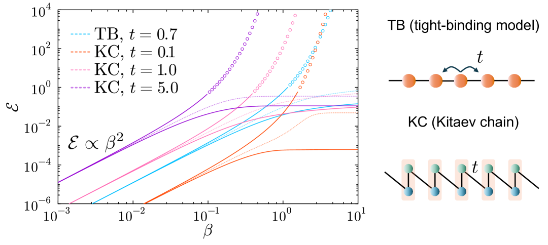
Figure 1: Universal bounds (14) on the negativity of the Gibbs states. The bounds (exact value) are shown in the solid (dotted) curve, with the circle marker denoting the regime $\|\Gamma_{AB}\|>k_{-}$, where the upper bound is not applicable. TB and KC correspond to the tight-binding chain and the Kitaev chain [45], respectively. In the Kitaev chain, $t=1$ is the critical value, and $t>1(<1)$ corresponds to the topological (trivial) phase at zero temperature. In both models, we take $N=20$ and adopt open boundary conditions. Also, we set the subsystem $A$ as half of the chain.

Bound on the negativity change rate.— Let us consider a time-evolving free-fermion state $\Gamma(t)$ and derive a bound on the negativity change rate $\partial_{t}\mathcal{E}(t)$. To this end, we first figure out the explicit formula for $\partial_{t}\mathcal{E}(t)$ from Eq. (8) as [34]

$$\partialderivative{\mathcal{E}(t)}{t}=\frac{1}{2}\Tr[\mathcal{P}_{AB}(\Gamma(t))\partialderivative{\Gamma(t)}{t}],$$ (15)

where $\mathcal{P}_{AB}$ is a superoperator defined by

$$\mathcal{P}_{AB}(\Gamma)=\int_{-\pi}^{\pi}\frac{dk}{2\pi}(Z_{AB}(k)+\Gamma)^{-1},$$ (16)

with $Z_{AB}(k)=e^{ik}\mathbb{I}_{A}\oplus(-e^{-ik})\mathbb{I}_{B}$ exhibiting a twist structure inheriting from Eq. (6). Note that $\partial_{t}\mathcal{E}(t)$ may become discontinuous at some specific time, when $\mathcal{P}_{AB}(\Gamma(t))$ becomes ill-defined. Nevertheless, we can show that $\|\mathcal{P}_{AB}(\Gamma)\|\leq 2$ whenever defined. By applying Hölder’s inequality, we can bound this change rate as [34]

$$\quantity|\partialderivative{\mathcal{E}(t)}{t}|\leq\left\|\partialderivative{\Gamma(t)}{t}\right\|_{1}.$$ (17)

Intuitively, this bound means the speed of entanglement change never exceeds that of the covariance matrix, which includes both intra- and inter-subsystem correlations.

Let us apply Eq. (17) to the Lindblad dynamics [47, 48]

$$\partialderivative{\hat{\rho}}{t}=-i[\hat{H},\hat{\rho}]+\sum_{\mu}\quantity(\hat{L}_{\mu}\hat{\rho}\hat{L}_{\mu}^{\dagger}-\frac{1}{2}\{\hat{L}_{\mu}^{\dagger}\hat{L}_{\mu},\hat{\rho}\}),$$ (18)

where $\hat{L}_{\mu}$ are the Lindblad operators arising from dissipation. We assume that the Lindblad operators are linear in the Majorana operators, so that the time-evolved states remain Gaussian [49, 50, 13]. Accordingly, the time-evolution of the states (18) is equivalently described by the equation of motion for the covariance matrix [49, 50, 13]:

$$\partialderivative{\Gamma}{t}=-i[4H,\Gamma]-\{X,\Gamma\}+2Y,$$ (19)

with $H$ being the Hamiltonian matrix, and $X=2B_{R}$, $Y=2iB_{I}$. Here $B_{R}$ and $B_{I}$ are the real and imaginary part of the matrix $B_{ij}=\sum_{\mu}L_{\mu,i}^{*}L_{\mu,j}$ determined from the Lindblad operators $\hat{L}_{\mu}=\sum_{j}L_{\mu,j}\hat{c}_{j}$. Combining Eq. (19) with Eq. (17), we arrive at

$$\quantity|\partialderivative{\mathcal{E}(t)}{t}|\leq 2(4\left\|H\right\|_{1}+\|X\|_{1}+\|Y\|_{1}),$$ (20)

where the right-hand side depends only on the Lindbladian.

This bound can be viewed as an open-system analogue of the small incremental entangling (SIE) theorem for unitary dynamics [30, 28]. It claims the absolute rate of change of entanglement entropy is upper bounded by $c\|\hat{H}_{AB}\|\ln d$, where $c$ is some $\mathcal{O}(1)$ constant, $\hat{H}_{AB}$ is the coupling Hamiltonian between two subsystems $A,B$, and $d=\min(d_{A},d_{B})$ with $d_{A(B)}$ denoting the local Hilbert-space dimension of $A(B)$ . Note that $d_{A(B)}=2^{N_{A(B)}}$ and $\|\hat{H}\|=\|H\|_{1}$ for $\hat{H}=\sum_{j,j^{\prime}}H_{j,j^{\prime}}\hat{c}_{j}\hat{c}_{j^{\prime}}$, so the results are indeed comparable except for an additional $\min(N_{A},N_{B})$ in the SIE bound.

We can even derive a tighter bound concerning the increase rate of entanglement by extracting the contribution from inter-subsystem hopping, pairing and dissipation. To this end, we utilize the fact that negativity rate (15) is linear with respect to $\partial_{t}\Gamma(t)$, which is in turn linear in the generators $H,X,Y$. Therefore, the negativity dynamics can be decomposed into contributions from intra-subsystem parts corresponding to local operations (LO) and inter-subsystem parts:

$$\partialderivative{\mathcal{E}}{t}=\left.\partialderivative{\mathcal{E}}{t}\right|_{\text{LO}}+\left.\partialderivative{\mathcal{E}}{t}\right|_{\text{inter}}.$$ (21)

Specifically, $\left.\partial_{t}\mathcal{E}(t)\right|_{\text{LO}}$ and $\left.\partial_{t}\mathcal{E}(t)\right|_{\text{inter}}$ are given by Eq. (15) with $H,X,Y$ in Eq. (19) replaced by their block-diagonal terms $H_{0},X_{0},Y_{0}$ and off-diagonal terms $H_{\text{inter}},X_{\text{inter}},Y_{\text{inter}}$, respectively. Since Local operations never increase the entanglement between $A$ and $B$ , the change rate of negativity is upper bounded by

$$\partialderivative{\mathcal{E}}{t}\leq\left.\partialderivative{\mathcal{E}}{t}\right|_{\text{inter}}.$$ (22)

Applying Eq. (17) to this inter-correlation term then yields

$$\partialderivative{\mathcal{E}}{t}\leq 2(4\|H_{\text{inter}}\|_{1}+\|X_{\text{inter}}\|_{1}+\|Y_{\text{inter}}\|_{1}).$$ (23)

Clustering property and area law of negativity.— Let us return to the static setup and discuss the entanglement area law of lattice systems with locality. Recently, significant progress has been made for extending the entanglement area law to systems with long-range interactions decaying by power-law [53, 27, 31, 54]. One notable feature of such systems is that the correlation functions exhibit the power-law decay at high temperatures [27, 54]. A fundamental question is to identify the minimal decay exponent for validating the area law. We approach this problem by using Eq. (14), which directly relates the clustering property and area law.

Suppose the system lives on a $D$-dimensional lattice $\Lambda$, and we have $j=(\bm{r},s)$ with $\bm{r}\in\Lambda$ denoting a lattice site and $s\in I$ labeling an internal degree of freedom. For long-range systems, we consider the following weak notion of clustering:

$$\|\Pi_{\bm{r}}\Gamma\Pi_{\bm{r}^{\prime}}\|\leq CF_{\alpha}(|\bm{r}-\bm{r}^{\prime}|),$$ (24)

where $\Pi_{\bm{r}}$ is the projector onto site $\bm{r}$, $C$ is an $\mathcal{O}(1)$ constant, and $F_{\alpha}(r)=(r+1)^{-\alpha}$ expresses power-law decay with its exponent $\alpha$. The key observation from our bound (14) is that the area law holds if and only if $\|\Gamma_{AB}\|_{2}^{2}=\sum_{\bm{r}\in A,\bm{r}^{\prime}\in B}\|\Pi_{\bm{r}}\Gamma\Pi_{\bm{r}^{\prime}}\|_{2}^{2}$ is proportional to its boundary $|\partial A|$, since $k_{\pm}$ and $\|\Gamma_{AB}\|$ are $\mathcal{O}(1)$ quantities with respect to the subsystem size. In $D$ dimensions, we can evaluate the summation using $g(r)=\int_{r}^{\infty}dRF(R)^{2}R^{D-1}$ and $G(r)=\int_{r}^{\infty}dRg(R)$ as [31]

$$\mathcal{E}\leq c_{g}C^{2}|I||\partial A|G(\text{dist}(A,B)),$$ (25)

where $c_{g}$ is an $\mathcal{O}(1)$ constant depending on the lattice geometry, and $\text{dist}(A,B)=\min\{|\bm{r}-\bm{r}^{\prime}|:\bm{r}\in A,\bm{r}^{\prime}\in B\}$ is the distance between subsystems $A$ and $B$. The area law follows as a special case with $B=\bar{A}$ and $\text{dist}(A,B)=1$. Therefore, we identify the area-law condition as $\alpha>(D+1)/2$, so that $G(1)$ is convergent. While this argument relies on the upper bound (12) conditioned on $\|\Gamma_{AB}\|\leq k_{-}$, the condition is easily justified when the state is sufficiently mixed, i.e., the purity $\tr[\hat{\rho}^{2}]$ is small enough.

Our result can be examined in Gibbs states $\hat{\rho}=e^{-\beta\hat{H}}/Z$ with $\hat{H}$ involving long-range hopping and pairing:

$$\|\Pi_{\bm{r}}H\Pi_{\bm{r}^{\prime}}\|\leq hF_{\alpha}(\|\bm{r}-\bm{r}^{\prime}\|),$$ (26)

with $\mathcal{O}(1)$ constant $h$. For $\alpha>D$, one can prove that the clustering property (24) follows from Eq. (26). While a rigorous proof is absent in the regime $\alpha\leq D$, the clustering property is numerically verified in Ref. [27] for various models. Since the condition for the upper bound $\|\Gamma_{AB}\|\leq k_{-}$ is easily satisfied in the high temperature regime, our argument concludes the condition for this thermal area law as $\alpha>(D+1)/2$, which confirms the conjecture in Ref. [27] based on numerical observations.

We remark that our argument only relies upon the clustering property. This implies, for example, that our argument could be extended to the nonequilibrium steady state of long-range Lindblad dynamics [47, 48, 55, 56].

Area law of negativity increase rate.— Finally, we establish a dynamical area law for the increase rate of negativity in Lindblad dynamics by utilizing our bound (23). More precisely, we will prove

$$\partialderivative{\mathcal{E}}{t}\leq\mathcal{O}(|\partial A|),$$ (27)

for the Lindblad dynamics (18) subject to locality constraints. Unlike the previous section, we do not assume the Gaussian state satisfies clustering or any other specific properties.

We emphasize a fundamental difference from similar statements for entanglement entropy in pure states in Refs. [29, 31] based on the SIE theorems. Therein, the area law of entanglement entropy rate holds for both increase and decrease rates, as the SIE theorem applies to both. In contrast, here the area law of negativity change rate should only be true for the increase rate, as shown in Fig. 2. This difference manifests in the difference between the bound for the increase rate (23) and that for the magnitude (17): while the former grows proportionally to the boundary size as far as the system is sufficiently local, the latter becomes proportional to the system size. For example, if one prepares a volume-law entangled initial state and considers particle-loss dynamics, then negativity clearly decreases proportionally to the subsystem size, not its boundary. Nevertheless, regarding the increase rate, we can prove an area law regardless of the initial state.

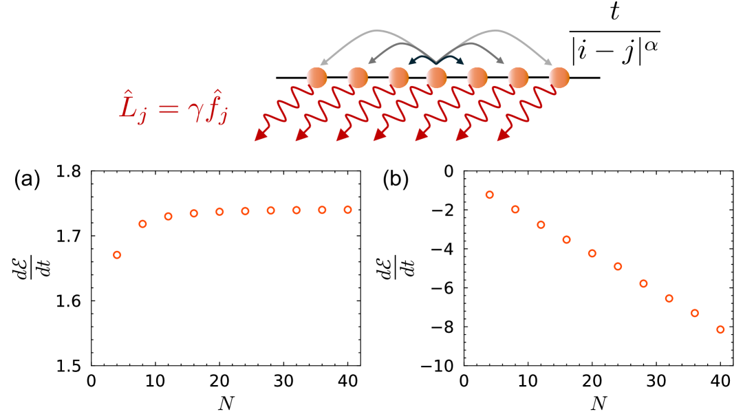
Figure 2: Change rate of negativity in a dissipative long-range hopping model with $t=1,\alpha=2.1$ and particle loss rate of $\gamma=0.5$. The system is one-dimensional with open boundary conditions, and the subsystem $A$ is half of the chain. The system is initialized in (a) a charge-density-wave state, $|\psi_{0}\rangle=(\prod_{j=1}^{N/2}\hat{f}_{2j}^{\dagger})|0\rangle$; (b) a randomly sampled (over 10000 realizations) mixed Gaussian state.

To prove the area law (27), we set the coefficients of Lindblad operators as $L_{\mu,j}=L_{(\bm{r},\nu),(\bm{r}^{\prime},s)}$, with $\nu\in J$ labeling the local dissipation channels. Let us impose the locality of dissipation as

$$\|\Pi_{\bm{r}}L\Pi_{\bm{r}^{\prime}}\|\leq lF_{\alpha}(|\bm{r}-\bm{r}^{\prime}|)$$ (28)

in addition to the locality of Hamiltonian (26), where $l$ is an $\mathcal{O}(1)$ constant and $L$ denotes the matrix of coefficients $L_{\mu,j}$. Assuming $\alpha>D$, this assumption (28) ensures the locality of $X,Y$ as

$$\|\Pi_{\bm{r}}X\Pi_{\bm{r}^{\prime}}\|,\|\Pi_{\bm{r}}Y\Pi_{\bm{r}^{\prime}}\|\leq 2c^{\prime}lF_{\alpha}(|\bm{r}-\bm{r}^{\prime}|)$$ (29)

by applying the self-production property $\sum_{\bm{r}}F_{\alpha}(|\bm{r}_{1}-\bm{r}|)F_{\alpha}(|\bm{r}-\bm{r}_{2}|)\leq c^{\prime}F_{\alpha}(|\bm{r}_{1}-\bm{r}_{2}|)$ [57], where $c^{\prime}$ is an $\mathcal{O}(1)$ constant. In this case, the area law holds if $\sum_{\bm{r}\in A,\bm{r}^{\prime}\in B}F_{\alpha}(|\bm{r}-\bm{r}^{\prime}|)$ is convergent. Since the summation can be evaluated in the same way as Eq. (25), $F_{\alpha}(r)$ should decay faster than $r^{-(D+1)}$ (i.e., $\alpha>D+1$). Note that the same condition was obtained for the dynamical area law of entanglement entropy shown in Ref. [31].

Our dynamical area law adds new insight into dissipation engineering. While engineered dissipation has been widely recognized as a quantum resource [58, 59, 60], it remains to understand whether introducing dissipation could surpass the unitary limit [61]. Our dynamical area law gives a no-go result regarding generation of bipartite entanglement. The absence of nonunitary advantage is already suggested by the similarity between the SIE and the bound for the increase change rate of entanglement (23).

Summary and outlook.— Focusing on free fermions, we have proposed the twisted characteristic polynomial to directly relate the entanglement negativity to the covariance matrix. Our formalism allows us to derive universal upper and lower bounds on negativity, which unveil the connection between the clustering of correlations and the entanglement area law. Moreover, we establish the first dynamical area law governing the entanglement negativity growth in local dissipative dynamics, revealing a fundamental universal constraint on entanglement generation beyond the unitary paradigm.

Several directions emerge for future work. One direction is to apply our formalism to topological insulators/superconductors at finite temperatures. In particular, it is intriguing to study how zeros of the twisted characteristic polynomial, as the counterpart of the entanglement spectrum [62], are related to topological phases. Furthermore, our framework can be applied to the entanglement structure of topological states that appear as steady states of engineered dissipative dynamics [50]. In particular, it is interesting to investigate how negativity characterizes these nonequilibrium topological phases and how it evolves under such dynamics.

Another natural question is whether our results can be generalized to interacting fermions. Very recently, it has been proved that general Gibbs states are mixtures of Gaussian states at high temperatures [40]. Therefore, we expect that the rigorous analysis of general interacting fermions may still benefit from our bounds.

Finally, a profound question concerns the meaning of “twist”. Since our twisted characteristic polynomial can be obtained from a partial modular transformation (i.e., $\lambda\to-\lambda^{-1}$) of the ordinary characteristic polynomial, it would be interesting to generalize our formula to $\mathbb{Z}_{n}$ parafermionic systems [63, 64] and to multipartite settings, where more blocks are expected to be twisted in different ways.

Supplemental Material for “Entanglement negativity in free fermions:
twisted characteristic polynomial, universal bounds and area laws”

SI Twisted characteristic polynomial

We review the logarithmic negativity for fermions proposed in [23], and show the derivation of our formula from the covariance matrix corresponding to the twisted partial transpose introduced in Ref. [25].

SI.1 Untwisted and twisted partial transpose

To state the definition of fermionic partial transpose, we begin by considering a general fermionic system with $N$ modes. The Hilbert space $\mathcal{H}$ is spanned by the Fock basis $\ket{n_{1},n_{2}\cdots,n_{N}}$, where $n_{j}=0,1$ is the occupation number of the $j$th mode. Any linear operator can be expressed in terms of creation and annihilation operators $\hat{f}_{j}^{\dagger}$ and $\hat{f}_{j}$, which act on the Fock basis as

$$\hat{f}_{j}\ket{n_{1},\cdots,n_{j},\cdots n_{N}}$$

$$\quad=\delta_{n_{j},1}(-1)^{\sum_{i=1}^{j-1}n_{i}}\ket{n_{1},\cdots,n_{j-1},0,n_{j+1},\cdots n_{N}},$$

$$\hat{f}_{j}^{\dagger}\ket{n_{1},\cdots,n_{j},\cdots n_{N}}$$

$$\quad=\delta_{n_{j},0}(-1)^{\sum_{i=1}^{j-1}n_{i}}\ket{n_{1},\cdots,n_{j-1},1,n_{j+1},\cdots n_{N}}.$$ (S1)

Due to (S1), $\hat{f}_{j}^{\dagger}$ and $\hat{f}_{j}$ satisfy the anticommutation relations

$$\{\hat{f}_{i},\hat{f}_{j}\}=\{\hat{f}_{i}^{\dagger},\hat{f}_{j}^{\dagger}\}=0\;,\{\hat{f}_{i},\hat{f}_{j}^{\dagger}\}=\delta_{ij},$$ (S2)

where $\{\hat{A},\hat{B}\}=\hat{A}\hat{B}+\hat{B}\hat{A}$.

For the definition of fermionic partial transpose, it is convenient to introduce a Majorana representation. Majorana operators $\hat{c}_{1},\cdots,\hat{c}_{2N}$ are constructed from the fermionic creation and annihilation operators as

$$\hat{c}_{2j-1}=\hat{f}_{j}+\hat{f}_{j}^{\dagger}\;,\;\hat{c}_{2j}=-i(\hat{f}_{j}-\hat{f}_{j}^{\dagger}),$$ (S3)

and satisfy $\{\hat{c}_{i},\hat{c}_{j}\}=2\delta_{ij}$. Any physical operator $\hat{X}$ acting on $\mathcal{H}$ is expressed in terms of polynomials of $\hat{c}_{j}$’s,

$$X=\sum_{k=1}^{2N}\sum_{p_{1}<p_{2}<\cdots<p_{k},k=\text{even}}X_{p_{1}\cdots p_{k}}\hat{c}_{p_{1}}\cdots\hat{c}_{p_{k}},$$ (S4)

where the restriction $k=\text{even}$ comes from the superselection rule.

To study the entanglement in a bipartite system, we divide the system into two subsystems A and B. The total Hilbert space is $\mathcal{H}=\mathcal{H}_{A}\otimes\mathcal{H}_{B}$, where $\mathcal{H}_{A}$ is generated by $\hat{c}_{j}$ with $j=1,\cdots,2N_{A}$ in subsystem A and $\mathcal{H}_{B}$ by $j=2N_{A}+1,\cdots,2N(=2(N_{A}+N_{B}))$ in subsystem B. Any physical state on $\mathcal{H}$ is given by

$$\hat{\rho}=\sum_{k_{1},k_{2}}^{k_{1}+k_{2}=\text{even}}\rho_{p_{1}\cdots p_{k_{1}},q_{1}\cdots q_{k_{2}}}\hat{a}_{p_{1}}\cdots\hat{a}_{p_{k_{1}}}\hat{b}_{q_{1}}\cdots\hat{b}_{q_{k_{2}}},$$ (S5)

where $\{\hat{a}_{j}\}$ and $\{\hat{b}_{j}\}$ are majorana operators acting on $\mathcal{H}_{A}$ and $\mathcal{H}_{B}$, respectively. Then, the untwisted partial transpose is defined as

$$\hat{\rho}^{\rm T_{A}}=\sum_{k_{1},k_{2}}^{k_{1}+k_{2}=\text{even}}\rho_{p_{1}\cdots p_{k_{1}},q_{1}\cdots q_{k_{2}}}i^{k_{1}}\hat{a}_{p_{1}}\cdots\hat{a}_{p_{k_{1}}}\hat{b}_{q_{1}}\cdots\hat{b}_{q_{k_{2}}}.$$ (S6)

This untwisted partial transpose preserves the tensor product structure (and thus the corresponding logarithmic negativity satisfies additivity) but not Hermiticity,

$$\quantity(\hat{\rho}^{\rm T_{A}})^{\dagger}=(-1)^{\hat{F}_{A}}\hat{\rho}^{\rm T_{A}}(-1)^{\hat{F}_{A}},$$ (S7)

where $\hat{F}_{A}=\sum_{j\in A}\hat{f}^{\dagger}_{j}\hat{f}_{j}$ is the number operator in A. This motivates us to introduce twisted partial transpose [25]

$$\hat{\rho}^{\tilde{\rm T}_{A}}=\hat{\rho}^{\rm T_{A}}(-1)^{\hat{F}_{A}},$$ (S8)

which is Hermitian by definition. Since $\|\hat{\rho}^{\rm T_{A}}\|_{1}=\|\hat{\rho}^{\tilde{\rm T}_{A}}\|_{1}$, it suffices to know the spectrum of $\hat{\rho}^{\tilde{\rm T}_{A}}$ to calculate logarithmic negativity.

SI.2 Covariance matrix of the twisted partial transpose

In the Gaussian case, it is rather convenient to apply twist partial transpose for the corresponding covariance matrix, and calculate logarithmic negativity from the covariance matrix for the twisted partial transpose $\tilde{\Gamma}$. Indeed, they are related as [25]

$$\mathcal{E} =\ln|\text{Pf}(\Gamma_{A})|+\sum_{j=1}^{N}\ln\max\{1,\tilde{\lambda}_{j}\},$$ (S9)

where $\pm\tilde{\lambda}_{j}\in\mathbb{R}\;(j=1,2,\cdots,N)$ are eigenvalues of $\tilde{\Gamma}$. Here we distinguish $\tilde{\lambda}_{j}$ from ${\lambda}_{j}$, which are the roots of the twisted characteristic polynomial $P(\lambda)$, but later it turns out that they are the same.

Let us move to calculate the explicit form of the covariance matrix for the twisted partial transpose $\tilde{\Gamma}$, based on the untwisted version given in Ref. [25]. We use the same bipartition for the original covariance matrix as (3) in the main text:

$$\Gamma=\begin{pmatrix}\Gamma_{A}&\Gamma_{AB}\\ \Gamma_{BA}&\Gamma_{B}\end{pmatrix}.$$ (S10)

Then, the covariance matrix of untwisted partial transpose $\hat{\rho}^{\rm T_{A}}$ and $\hat{\rho}{{}^{\rm T_{A}}}^{\dagger}$ is given by [25]

$$\Gamma_{\pm}=\begin{pmatrix}-\Gamma_{A}&\pm i\Gamma_{AB}\\ \pm i\Gamma_{BA}&\Gamma_{B}\end{pmatrix},$$ (S11)

where $\pm$ correspond to $\hat{\rho}^{\rm T_{A}}$ and $\hat{\rho}{{}^{\rm T_{A}}}^{\dagger}$. As for the twisted partial transpose $\hat{\rho}^{\tilde{\rm T}_{A}}=\hat{\rho}^{\rm T_{A}}(-1)^{\hat{F}_{A}}$ and $\hat{\rho}^{{\rm T_{A}}^{\dagger}}(-1)^{\hat{F}_{A}}$, we have [25]

$$e^{\tilde{\Omega}_{\pm}}=\frac{\mathbb{I}+\Gamma_{\pm}}{\mathbb{I}-\Gamma_{\pm}}U_{A},\;\;\;U_{A}=\begin{pmatrix}-\mathbb{I}_{A}&0\\ 0&\mathbb{I}_{B}\end{pmatrix}.$$ (S12)

Substituting Eq. (S12) into $\tilde{\Gamma}_{\pm}=\tanh\frac{\tilde{\Omega}_{\pm}}{2}$, we obtain

$$\tilde{\Gamma}=\frac{e^{\tilde{\Omega}_{\pm}}-\mathbb{I}}{e^{\tilde{\Omega}_{\pm}}+\mathbb{I}} =[(\mathbb{I}-\Gamma_{\pm})^{-1}(\mathbb{I}+\Gamma_{\pm})U_{A}+\mathbb{I}]^{-1}[(\mathbb{I}-\Gamma_{\pm})^{-1}(\mathbb{I}+\Gamma_{\pm})U_{A}-\mathbb{I}]$$

$$=[(\mathbb{I}+\Gamma_{\pm})U_{A}+(\mathbb{I}-\Gamma_{\pm})]^{-1}[(\mathbb{I}+\Gamma_{\pm})U_{A}-(\mathbb{I}-\Gamma_{\pm})]$$

$$=(\Pi_{B}-\Gamma_{\pm}\Pi_{A})^{-1}(\Gamma_{\pm}\Pi_{B}-\Pi_{A}),$$ (S13)

where we used $2\Pi_{A}=\mathbb{I}-U_{A}$ and $2\Pi_{B}=\mathbb{I}+U_{A}$. Since $\Pi_{A,B}$ is the projector onto $A,B$, we can explicitly write down the block forms as

$$\Pi_{B}-\Gamma_{\pm}\Pi_{A}=\begin{pmatrix}\Gamma_{A}&0\\ \mp i\Gamma_{BA}&\mathbb{I}_{B}\end{pmatrix},\Gamma_{\pm}\Pi_{B}-\Pi_{A}=\begin{pmatrix}-\mathbb{I}_{A}&\pm i\Gamma_{AB}\\ 0&\Gamma_{B}\end{pmatrix}.$$ (S14)

Assuming the invertibility of $\Gamma_{A}$, the inverse of the former turns out to be

$$(\Pi_{B}-\Gamma_{\pm}\Pi_{A})^{-1}=\begin{pmatrix}\Gamma_{A}^{-1}&0\\ \pm i\Gamma_{BA}\Gamma_{A}^{-1}&\mathbb{I}_{B}\end{pmatrix}.$$ (S15)

Therefore, by substituting Eqs. (S14) and (S15) into Eq. (S13), we can derive the covariance matrix corresponding to $\hat{\rho}^{\tilde{\rm T}_{A}}=\hat{\rho}^{\rm T_{A}}(-1)^{\hat{F}_{A}}$ and $\hat{\rho}^{{\rm T_{A}}^{\dagger}}(-1)^{\hat{F}_{A}}$ as

$$\tilde{\Gamma}_{\pm}=\begin{pmatrix}-\Gamma_{A}^{-1}&\pm i\Gamma_{A}^{-1}\Gamma_{AB}\\ \mp i\Gamma_{BA}\Gamma_{A}^{-1}&\Gamma_{B}-\Gamma_{BA}\Gamma_{A}^{-1}\Gamma_{AB}\end{pmatrix}.$$ (S16)

SI.3 Derivation of twisted characteristic polynomial

Finally, we show the equivalence of the formula (S9) and our formula (8), under the assumption of the invertibility of $\Gamma_{A}$. Using the invariance of determinant under column linear operations (or right multiplying the upper triangle matrix $\begin{pmatrix}\mathbb{I}_{A}&\mp i\Gamma_{AB}\\ 0&\mathbb{I}_{B}\end{pmatrix}$ with unit determinant), we have

$$\det(\tilde{\Gamma}_{\pm}-\lambda\mathbb{I})=\det\begin{pmatrix}-\Gamma_{A}^{-1}-\lambda\mathbb{I}_{A}&\mp i\lambda\Gamma_{AB}\\ \mp i\Gamma_{BA}\Gamma_{A}^{-1}&\Gamma_{B}-\lambda\mathbb{I}_{B}\end{pmatrix}.$$ (S17)

Note that

$$\begin{pmatrix}-\Gamma_{A}^{-1}-\lambda\mathbb{I}_{A}&\mp i\lambda\Gamma_{AB}\\ \mp i\Gamma_{BA}\Gamma_{A}^{-1}&\Gamma_{B}-\lambda\mathbb{I}_{B}\end{pmatrix}=\begin{pmatrix}\lambda\mathbb{I}_{A}&0\\ 0&\pm i\mathbb{I}_{B}\end{pmatrix}\begin{pmatrix}\Gamma_{A}+\lambda^{-1}\mathbb{I}_{A}&\Gamma_{AB}\\ \Gamma_{BA}&\Gamma_{B}-\lambda\mathbb{I}_{B}\end{pmatrix}\begin{pmatrix}-\Gamma_{A}^{-1}&0\\ 0&\mp i\mathbb{I}_{B}\end{pmatrix},$$ (S18)

as long as $\Gamma_{A}$ is invertible. This implies

$$P(\lambda)=\det(\Gamma_{A})\det(\tilde{\Gamma}_{\pm}-\lambda\mathbb{I}),$$ (S19)

where $P(\lambda)$ is the twisted characteristic polynomial given in Eq. (6). One can see that the coefficient of the leading term $\lambda^{2N}$ is exactly $\det(\Gamma_{A})=\text{Pf}(\Gamma_{A})^{2}$, according to which Eq. (8) follows. As the coefficients in $P(\lambda)$ depend continuously on $\Gamma_{A}$, the zeros should also have a continuous dependence. This justifies the continuity of Eq. (8) in terms of $\Gamma_{A}$ regardless of its invertibility.

SI.4 two modes example

We demonstrate our formula in the simplest two fermionic modes example. First we treat Gibbs state given by the Hamiltonian

$$\hat{H}=-J(\hat{f}_{2}^{\dagger}\hat{f}_{1}+\text{H.c.}),$$ (S20)

which is also treated in appendix of Ref. [67]. One can check that the Gibbs state is determined by $\Omega=\beta J\sigma_{x}\otimes\sigma_{y}$, so that $\Gamma=\tanh(\frac{\beta J}{2})\sigma_{x}\otimes\sigma_{y}$. The twisted characteristic polynomial for the two-mode entanglement reads

$$P(\lambda)=\quantity(1+\tanh^{2}\quantity(\frac{\beta J}{2}))^{2}\lambda^{2},$$ (S21)

whose roots (simply 0) are smaller than 1. This implies

$$\mathcal{E}(\beta)=\ln\quantity(\frac{2\cosh(\beta J)}{1+\cosh(\beta J)}).$$ (S22)

This result is exactly the same in Ref. [67], where this result is derived by expanding $\hat{{\rho}}$ in fock basis and directly apply the partial transpose in each matrix elements. The asymptotic form in the high temperature limit reads $\mathcal{E}(\beta)=(\beta J)^{2}/4+\mathcal{O}\quantity((\beta J)^{4})$, which is consistent with the universal scaling obtained by our bounds.

Next, we treat the dissipative dynamics of two fermionic modes, which can be thought as a counterpart of (S20) in the sense of entanglement sudden death. We take the initial entangled state $\frac{1}{\sqrt{2}}(\hat{f}_{1}^{\dagger}+\hat{f}_{2}^{\dagger})\ket{0}$, whose covariance matrix is

$$\Gamma_{0}=\sigma_{x}\otimes\sigma_{y}=\begin{pmatrix}0&\sigma_{y}\\ \sigma_{y}&0\end{pmatrix}.$$ (S23)

Note that this initial state is nothing but the ground state of the previous two-mode Hamiltonian (S20). The dynamics is described by the Lindblad operators $\hat{L}_{1}=\sqrt{\gamma_{1}}\hat{f}_{1}$ and $\hat{L}_{2}=\sqrt{\gamma_{2}}\hat{f}_{2}$ with decay rates $\gamma_{1}$ and $\gamma_{2}$, and we take $\gamma_{1}=\gamma_{2}=\gamma$ to simplify our calculation. Then the $X,Y$ defined in Eq. (19) is $X=\frac{\gamma}{2}\mathbb{I}_{4},Y=-\frac{\gamma}{2}\sigma_{y}^{\oplus 2}$. Therefore

$$\Gamma(t)=e^{-\gamma t}(\Gamma_{0}+\sigma_{y}^{\oplus 2})-\sigma_{y}^{\oplus 2}=\begin{pmatrix}-\sigma_{y}(1-e^{-\gamma t})&\sigma_{y}e^{-\gamma t}\\ \sigma_{y}e^{-\gamma t}&-\sigma_{y}(1-e^{-\gamma t})\end{pmatrix},$$ (S24)

which yields the twisted characteristic polynomial

$$P(\lambda;t)=-(1-e^{-\gamma t})^{2}\quantity[\lambda^{4}-2\quantity(\frac{2e^{-2\gamma t}}{(1-e^{-\gamma t})^{2}}+1)\lambda^{2}+1].$$ (S25)

In $t>0$, the roots of (S25) are

$$\lambda_{\pm}(t)=\sqrt{b(t)\pm\sqrt{b(t)^{2}-1}},\;b(t)=\frac{2e^{-2\gamma t}}{(1-e^{-\gamma t})^{2}}+1,$$ (S26)

and $0<\lambda_{-}(t)<1<\lambda_{+}(t)$ because $b(t)>1$. Thus, the exact solution of negativity is

$$\mathcal{E}(t) =\frac{1}{2}\ln|P_{>}(0;t)|=\frac{1}{2}\ln\quantity[(1-e^{-t})^{2}(b(t)+\sqrt{b(t)^{2}-1})]$$

$$=\frac{1}{2}\ln\quantity[2e^{-2\gamma t}+(1-e^{-\gamma t})^{2}+2e^{-\gamma t}\sqrt{e^{-2\gamma t}+(1-e^{-\gamma t})^{2}}].$$ (S27)

Since (S27) satisfies $\mathcal{E}(0)=\ln 2$, this is true for $t\geq 0$. We can derive the asymptotic form of (S27) as

$$\mathcal{E}(t)=\begin{cases}\ln 2-\gamma t+\mathcal{O}((\gamma t)^{2})&\text{when $t\to 0$,}\\ \frac{1}{2}e^{-2\gamma t}+\mathcal{O}(e^{-3\gamma t})&\text{when $t\to\infty$.}\end{cases}$$ (S28)

We show these two cases in Fig. S1.

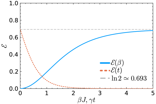
Figure S1: Exact negativity of the Gibbs state (S22) and of the dissipative dynamics (S27).

SII Universal bounds on negativity

SII.1 Derivation of the bounds

In this section, we show how to derive the upper and lower bounds of negativity, Eq. (12) and (13) in the main text.

A general Gaussian operation is in the form of Eq. (10), and here we consider the specific Gaussian channel with $D=0$ and $K=i\sqrt{k}\mathbb{I}\;(k\geq 0)$ such that

$$\Gamma_{\text{out}}=k\Gamma_{\text{in}}+C.$$ (S29)

The constraint in Eq. (11) reads

$$\left|\left|\frac{\sigma_{z}+\sigma_{0}}{2}\otimes C-\sqrt{k}\sigma_{y}\otimes\mathbb{I}\right|\right|=\frac{1}{2}\quantity(\|C\|+\sqrt{\|C\|^{2}+4k})\leq 1,$$ (S30)

which is equivalent to

$$k\leq 1-\|C\|,\|C\|\leq 1.$$ (S31)

To derive the upper bound (12), we choose

$$\Gamma_{\text{in}}=k^{-1}\begin{pmatrix}0&\Gamma_{AB}\\ \Gamma_{BA}&0\end{pmatrix},C=\Gamma_{A}\oplus\Gamma_{B},$$ (S32)

so that $\Gamma_{\text{out}}$ is exactly the state of interest. In this case, $\|C\|=\max\{\|\Gamma_{A}\|,\|\Gamma_{B}\|\}$ and there is additional constraint $\|\Gamma_{\text{in}}\|\leq 1\Leftrightarrow\|\Gamma_{AB}\|\leq k$. The logarithmic entanglement negativity of the input state is given by

$$\mathcal{E}_{\text{in}}=\frac{1}{2}\tr[\ln(\mathbb{I}_{B}+k_{-}^{-2}\Gamma_{BA}\Gamma_{AB})],$$ (S33)

so the tightest version is $k=1-\max\{\|\Gamma_{A}\|,\|\Gamma_{B}\|\}$ with further constraint $k_{-}\leq\|\Gamma_{AB}\|$.

To derive the lower bound (13), we choose

$$\Gamma_{\text{in}}=\Gamma,C=-k(\Gamma_{A}\oplus\Gamma_{B}).$$ (S34)

In this case, $\|C\|=k\max\{\|\Gamma_{A}\|,\|\Gamma_{B}\|\}$ and the only constraint is

$$k\leq(1+\max{\|\Gamma_{A}\|,\|\Gamma_{B}\|})^{-1}.$$ (S35)

The lower bound is given by the entanglement negativity of the output state:

$$\mathcal{E}_{\text{out}}=\frac{1}{2}\tr[\ln(\mathbb{I}_{B}+k_{+}^{2}\Gamma_{BA}\Gamma_{AB})]$$ (S36)

which is maximized by $k=k_{+}^{-1}$.

We emphasize these bounds should be far from optimal because our choices are rather specific (yet make the calculations extremely simple). For example, there is an obvious improvement for the lower bound by choosing C to be either $-k\Gamma_{A}\oplus 0$ or $0\oplus(-k\Gamma_{B})$, so that $k_{+}$ in Eq. (13) can be replaced by $1+\min\{\|\Gamma_{A}\|,\|\Gamma_{B}\|\}$.

SII.2 Numerical calculation of the bounds

For the numerical verification of our bounds, we employed two different models and calculated the bounds and exact negativity of the Gibbs state of those models. The models are tight-binding model and Kitaev chain with open boundary condition, whose Hamiltonians are given by

$$\hat{H}_{\text{TB}} =-\sum_{i=1}^{N-1}t(\hat{f}^{\dagger}_{i}\hat{f}_{i+1}+\text{H.c.})=\sum_{i=1}^{N-1}\frac{it}{2}(\hat{c}_{2i}\hat{c}_{2i+1}-\hat{c}_{2i-1}\hat{c}_{2i+2}),$$ (S37)

$$\hat{H}_{\text{Kitaev}} =-\sum_{i=1}^{N-1}t(\hat{f}^{\dagger}_{i}-\hat{f}_{i})(\hat{f}_{i+1}^{\dagger}+\hat{f}_{i+1})-2\sum_{i=1}^{N}\quantity(\hat{f}_{i}^{\dagger}\hat{f}_{i}-\frac{1}{2})=-\sum_{i=1}^{N}i\hat{c}_{2i-1}\hat{c}_{2i}+\sum_{i=1}^{N-1}it\hat{c}_{2i}\hat{c}_{2i+1}.$$ (S38)

In the main text, we showed that our bound exactly captures the universal behavior of the free-fermion negativity in the high temperature regime. However, we note that our bounds (14) are far from optimal in the low temperature regime. We observed that the behavior is qualitatively the same if we employ tighter bounds (12) and (13). We expect that bounds can be further improved by making a better choice of Gaussianity-preserving local operations.

SIII The change rate of negativity

SIII.1 Derivation of the formula for the change rate of negativity

We show the derivation of the explicit formula of negativity change rate $\partial_{t}\mathcal{E}(t)$. We write time dependence of the twisted characteristic polynomial (6) as $P(\lambda;t)=\det(\Gamma_{A}(t))\prod_{j=1}^{2N}(\lambda-\lambda_{j}(t))$. Then, the time derivative of Eq. (8) reads

$$\partialderivative{\mathcal{E}}{t} =\frac{1}{2}\quantity(\frac{\partial_{t}\det(\Gamma_{A}(t))}{\det(\Gamma_{A}(t))}+\sum_{j:|\lambda_{j}|>1}\frac{\partial_{t}\lambda_{j}(t)}{\lambda_{j}(t)})$$

$$=\frac{1}{2}\int_{-\pi}^{\pi}\frac{dk}{2\pi}\frac{\partial_{t}P(e^{-ik};t)}{P(e^{-ik};t)}=\frac{1}{2}\int_{-\pi}^{\pi}\frac{dk}{2\pi}\partial_{t}\ln P(e^{-ik};t),$$ (S39)

where we used an integral

$$\int_{-\pi}^{\pi}\frac{dk}{2\pi}\frac{1}{\lambda_{j}-e^{-ik}}=\begin{cases}0&\text{if $|\lambda_{j}|<1$,}\\ \frac{1}{\lambda_{j}}&\text{if $|\lambda_{j}|>1$}.\end{cases}$$ (S40)

To proceed, we define matrix $\Xi$ by $P(\lambda;t)=\det\Xi(\lambda;t)$. Since

$$\partial_{t}\ln P(e^{-ik};t) =\partial_{t}\ln\det\Xi(e^{-ik};t)$$

$$=\Tr[\Xi^{-1}(e^{-ik};t)\partialderivative{t}\Xi(e^{-ik};t)],$$ (S41)

and $\Xi$ is related to the covariance matrix $\Gamma$ via

$$\Xi(\lambda;t) =U(\lambda)(V(\lambda)+\Gamma(t)),$$

$$U(\lambda) =\begin{pmatrix}\lambda\mathbb{I}_{A}&0\\ 0&\mathbb{I}_{B}\end{pmatrix},V(\lambda)=\begin{pmatrix}\lambda^{-1}\mathbb{I}_{A}&0\\ 0&-\lambda\mathbb{I}_{B}\\ \end{pmatrix},$$ (S42)

we arrive at the explicit formula of negativity rate:

$$\partialderivative{\mathcal{E}}{t}=\frac{1}{2}\int_{-\pi}^{\pi}\frac{dk}{2\pi}\Tr[\quantity(V(e^{-ik})+\Gamma(t))^{-1}\partialderivative{\Gamma(t)}{t}].$$ (S43)

Therefore, denoting $Z_{AB}(k)=V(e^{-ik})=e^{ik}\mathbb{I}_{A}\oplus(-e^{-ik})\mathbb{I}_{B}$, we derive Eq. (15) in the main text:

$$\partialderivative{\mathcal{E}}{t}=\frac{1}{2}\Tr\left[\mathcal{P}_{AB}(\Gamma)\partialderivative{\Gamma}{t}\right],\;\;\;\mathcal{P}_{AB}(\Gamma)=\int^{\pi}_{-\pi}\frac{dk}{2\pi}(Z_{AB}(k)+\Gamma)^{-1}.$$ (S44)

SIII.2 Block diagonal representation

To gain further insights into $\mathcal{P}_{AB}$, it turns out to be helpful to go back to the formalism presented in Ref. [25]. We first rewrite $\mathcal{P}_{AB}(\Gamma)$ into a contour integral along a unit circle:

$$\mathcal{P}_{AB}(\Gamma)=\oint_{|z|=1}\frac{dz}{2\pi i}\begin{bmatrix}z^{2}+z\Gamma_{A}&z\Gamma_{AB}\\ z\Gamma_{BA}&z\Gamma_{B}-1\end{bmatrix}^{-1}.$$ (S45)

By slightly deforming the integral contour, we can make the integrand matrix invertible and apply the matrix inverse formula for block matrices. The diagonal block restricted to $A$ reads

$$\begin{split}P_{A}\mathcal{P}_{AB}(\Gamma)P_{A}&=\oint_{|z|=1}\frac{dz}{2\pi i}(z^{2}+z\Gamma_{A}-z^{2}\Gamma_{AB}(z\Gamma_{B}-1)^{-1}\Gamma_{BA})^{-1}\\ &=\oint_{|\zeta|=1}\frac{d\zeta}{2\pi i}(1+\Gamma_{AB}\Gamma_{BA}+\zeta\Gamma_{A}-\Gamma_{AB}(1-\zeta\Gamma_{B}^{-1})^{-1}\Gamma_{BA})^{-1}\\ &=\oint_{|\zeta|=1}\frac{d\zeta}{2\pi i}P_{A}\begin{bmatrix}\zeta\Gamma_{A}+\Gamma_{AB}\Gamma_{BA}+1&\Gamma_{AB}\\ \Gamma_{BA}&-\zeta\Gamma_{B}^{-1}+1\end{bmatrix}^{-1}P_{A}\\ &=\oint_{|\zeta|=1}\frac{d\zeta}{2\pi i}P_{A}\left(1+\zeta\begin{bmatrix}\Gamma_{A}-\Gamma_{AB}\Gamma_{B}^{-1}\Gamma_{BA}&\Gamma_{AB}\Gamma_{B}^{-1}\\ \Gamma_{B}^{-1}\Gamma_{BA}&-\Gamma_{B}^{-1}\end{bmatrix}\right)^{-1}P_{A}.\end{split}$$ (S46)

Here we have further assumed $\Gamma_{B}$ is invertible, and in the last line we have used

$$\begin{bmatrix}\Gamma_{AB}\Gamma_{BA}+1&\Gamma_{AB}\\ \Gamma_{BA}&1\end{bmatrix}=\begin{bmatrix}1&\Gamma_{AB}\\ 0&1\end{bmatrix}\begin{bmatrix}1&0\\ \Gamma_{BA}&1\end{bmatrix},\;\;\;\;\begin{bmatrix}1&\Gamma_{AB}\\ 0&1\end{bmatrix}^{-1}=\begin{bmatrix}1&-\Gamma_{AB}\\ 0&1\end{bmatrix},\;\;\;\;\begin{bmatrix}1&-\Gamma_{AB}\\ 0&1\end{bmatrix}P_{A}=P_{A}.$$ (S47)

Likewise, we can obtain the diagonal block restricted to $B$ (under the assumption that $\Gamma_{A}$ is invertible):

$$\begin{split}P_{B}\mathcal{P}_{AB}(\Gamma)P_{B}&=\oint_{|\zeta|=1}\frac{d\zeta}{2\pi i}P_{B}\begin{bmatrix}-\zeta\Gamma_{A}^{-1}+1&\Gamma_{AB}\\ \Gamma_{BA}&\zeta\Gamma_{B}+\Gamma_{BA}\Gamma_{AB}+1\end{bmatrix}^{-1}P_{B}\\ &=\oint_{|\zeta|=1}\frac{d\zeta}{2\pi i}P_{B}\left(1+\zeta\begin{bmatrix}-\Gamma_{A}^{-1}&\Gamma_{A}^{-1}\Gamma_{AB}\\ \Gamma_{BA}\Gamma_{A}^{-1}&\Gamma_{B}-\Gamma_{BA}\Gamma_{A}^{-1}\Gamma_{AB}\end{bmatrix}\right)^{-1}P_{B}.\end{split}$$ (S48)

In contrast, the off-diagonal block reads

$$\begin{split}P_{A}\mathcal{P}_{AB}(\Gamma)P_{B}&=\oint_{|z|=1}\frac{dz}{2\pi i}(z+\Gamma_{A}-z\Gamma_{AB}(z\Gamma_{B}-1)^{-1}\Gamma_{BA})^{-1}\Gamma_{AB}(1-z\Gamma_{B})^{-1}\\ &=\oint_{|z|=1}\frac{dz}{2\pi i}(z+\Gamma_{A}-\Gamma_{AB}\Gamma_{B}^{-1}\Gamma_{BA}-\Gamma_{AB}\Gamma_{B}^{-1}(z-\Gamma_{B}^{-1})^{-1}\Gamma_{B}^{-1}\Gamma_{BA})^{-1}\Gamma_{AB}\Gamma_{B}^{-1}(\Gamma_{B}^{-1}-z)^{-1}\\ &=\oint_{|z|=1}\frac{dz}{2\pi i}P_{A}\left(z+\begin{bmatrix}\Gamma_{A}-\Gamma_{AB}\Gamma_{B}^{-1}\Gamma_{BA}&\Gamma_{AB}\Gamma_{B}^{-1}\\ \Gamma_{B}^{-1}\Gamma_{BA}&-\Gamma_{B}^{-1}\end{bmatrix}\right)^{-1}P_{B},\end{split}$$ (S49)

whose Hermitian conjugation gives the other off-diagonal block:

$$P_{A}\mathcal{P}_{AB}(\Gamma)P_{B}=(P_{B}\mathcal{P}_{AB}(\Gamma)P_{A})^{\dagger}.$$ (S50)

SIII.3 Universal bound

It is clear from the matrices in the above block formulas are closely related to

$$\tilde{\Gamma}_{\pm}=\begin{bmatrix}-\Gamma_{A}^{-1}&\pm i\Gamma_{A}^{-1}\Gamma_{AB}\\ \mp i\Gamma_{BA}\Gamma_{A}^{-1}&\Gamma_{B}-\Gamma_{BA}\Gamma_{A}^{-1}\Gamma_{AB}\end{bmatrix},$$ (S51)

as well as the inverse

$$\tilde{\Gamma}_{\pm}^{-1}=\begin{bmatrix}-\Gamma_{A}+\Gamma_{AB}\Gamma_{B}^{-1}\Gamma_{BA}&\pm i\Gamma_{AB}\Gamma_{B}^{-1}\\ \mp i\Gamma_{B}^{-1}\Gamma_{BA}&\Gamma_{B}^{-1}\end{bmatrix}.$$ (S52)

Indeed, we can rewrite the diagonal blocks as

$$P_{A}\mathcal{P}_{AB}(\Gamma)P_{A}=\oint_{|\zeta|=1}\frac{d\zeta}{2\pi i}P_{A}(1-\zeta\tilde{\Gamma}_{\pm}^{-1})^{-1}P_{A},\;\;\;\;P_{B}\mathcal{P}_{AB}(\Gamma)P_{B}=\oint_{|\zeta|=1}\frac{d\zeta}{2\pi i}P_{B}(1-\zeta\tilde{\Gamma}_{\pm})^{-1}P_{B},$$ (S53)

and the off-diagonal blocks as

$$P_{A}\mathcal{P}_{AB}(\Gamma)P_{B}=\pm i\oint_{|\zeta|=1}\frac{d\zeta}{2\pi i}P_{A}(z-\tilde{\Gamma}_{\pm}^{-1})^{-1}P_{B}.$$ (S54)

Note that one can choose either branch of $\tilde{\Gamma}_{\pm}$ since $\tilde{\Gamma}_{+}=Z_{AB}\tilde{\Gamma}_{-}Z_{AB}$ ($Z_{AB}=\mathbb{I}_{A}\oplus(-\mathbb{I}_{B})=Z_{AB}(0)$) and $P_{A}Z_{AB}=P_{A}$, $P_{B}Z_{AB}=-P_{B}$. Denoting $P^{<}_{\pm}$ / $P^{>}_{\pm}$ as the projector onto the subspace spanned by all the eigenvectors of $\tilde{\Gamma}_{\pm}$ with eigenvalues whose absolute values are smaller / greater than $1$, we have $P^{<}_{\pm}+P^{>}_{\pm}=1$, $P^{>,<}_{\pm}=Z_{AB}P^{>,<}_{\mp}Z_{AB}$ and

$$P_{A}\mathcal{P}_{AB}(\Gamma)P_{A}=-P_{A}P^{<}_{\pm}\tilde{\Gamma}_{\pm}P_{A},\;\;\;\;P_{B}\mathcal{P}_{AB}(\Gamma)P_{B}=-P_{B}P^{>}_{\pm}\tilde{\Gamma}_{\pm}^{-1}P_{B},\;\;\;\;P_{A}\mathcal{P}_{AB}(\Gamma)P_{B}=\pm iP_{A}P^{>}_{\pm}P_{B}.$$ (S55)

Note that $\|P^{<}_{\pm}\tilde{\Gamma}_{\pm}\|\leq 1$ and $\|P^{>}_{\pm}\tilde{\Gamma}_{\pm}^{-1}\|\leq 1$, we have

$$\|\mathcal{P}_{AB}(\Gamma)\|\leq\|P_{A}\mathcal{P}_{AB}(\Gamma)P_{A}+P_{B}\mathcal{P}_{AB}(\Gamma)P_{B}\|+\|P_{A}\mathcal{P}_{AB}(\Gamma)P_{B}+P_{B}\mathcal{P}_{AB}(\Gamma)P_{A}\|\leq 2.$$ (S56)

Recalling Eq. (S44) and applying Hölder inequality, we end up with the bound on the negativity change rate (Eq. (17) in the main text):

$$\left|\partialderivative{\mathcal{E}}{t}\right|\leq\left\|\partialderivative{\Gamma}{t}\right\|_{1}.$$ (S57)

We remark that while the derivation above appears to rely on the invertibility of $\Gamma_{A,B}$, we expect the result to remain valid in general. This is because the divergence should never appear in the final expression due to the projection $P^{<,>}_{\pm}$. We may also understand the singularity in the negativity dynamics from the ambiguity of $P^{<,>}_{\pm}$ in case that some eigenvalues of $\tilde{\Gamma}_{\pm}$ are exactly of norm $1$. Again, even though $\partial_{t}\mathcal{E}(t)$ becomes discontinuous, the above bound remains valid. Finally, we mention that Eq. (S57) is probably not optimal, i.e., there could be some coefficient smaller than 1 in the right-hand side.

SIII.4 Monotonicity under local operations

On the level of covariance matrix, a general continuous-time Gaussianity-preserving evolution is given by Eq. (19):

$$\partialderivative{\Gamma}{t}=-i[h,\Gamma]-\{X,\Gamma\}+2Y,$$ (S58)

where $h=4H$ is a purely imaginary anti-symmetric matrix, and $X={\rm Re}M$, $Y=i{\rm Im}M$ with $M=2B$ being a positive semi-definite matrix. This time evolution becomes a local operation if

$$h=h_{A}\oplus h_{B},\;\;\;\;X=X_{A}\oplus X_{B},\;\;\;\;Y=Y_{A}\oplus Y_{B},$$ (S59)

i.e., only block-diagonal components can be nonzero in these matrices. Substituting Eq. (S58) into Eq. (S44), we will encounter terms like

$$\mathcal{P}_{AB}(\Gamma)\Gamma=1-\int^{\pi}_{-\pi}\frac{dk}{2\pi}(1+Z_{AB}(k)\Gamma)^{-1},\;\;\;\;\Gamma\mathcal{P}_{AB}(\Gamma)=1-\int^{\pi}_{-\pi}\frac{dk}{2\pi}(1+\Gamma Z_{AB}(k))^{-1}.$$ (S60)

Introducing

$$\mathcal{L}_{AB}(\Gamma)=\int^{\pi}_{-\pi}\frac{dk}{2\pi}(1+Z_{AB}(k)\Gamma)^{-1},\;\;\;\;\mathcal{R}_{AB}(\Gamma)=\int^{\pi}_{-\pi}\frac{dk}{2\pi}(1+\Gamma Z_{AB}(k))^{-1}=\mathcal{L}_{AB}(\Gamma)^{\dagger},$$ (S61)

we can perform similar calculations as for $\mathcal{P}_{AB}(\Gamma)$ previously, obtaining

$$\begin{split}P_{A}\mathcal{L}_{AB}(\Gamma)P_{A}&=\oint_{|\zeta|=1}\frac{d\zeta}{2\pi i}P_{A}(\zeta-\tilde{\Gamma}_{\pm}^{-1})^{-1}P_{A}=P_{A}P^{>}_{\pm}P_{A},\\ P_{B}\mathcal{L}_{AB}(\Gamma)P_{B}&=\oint_{|z|=1}\frac{dz}{2\pi i}P_{B}(z-\tilde{\Gamma}_{\pm})^{-1}P_{B}=P_{B}P^{<}_{\pm}P_{B},\\ P_{B}\mathcal{L}_{AB}(\Gamma)P_{A}&=(P_{A}\mathcal{L}_{AB}(\Gamma)P_{B})^{\dagger}=\pm i\oint_{|\zeta|=1}\frac{d\zeta}{2\pi i}P_{B}(1-\zeta\tilde{\Gamma}_{\pm})^{-1}P_{A}=\mp iP_{B}P^{>}_{\pm}\tilde{\Gamma}_{\pm}^{-1}P_{A}.\end{split}$$ (S62)

Recalling Eq. (S59) in the case of local operations, we find that $d\mathcal{E}/dt$ cannot increase:

$$\begin{split}\partialderivative{\mathcal{E}}{t}&=-\Tr[X]+\Tr[P^{>}_{\pm}X_{A}]+\Tr[P^{<}_{\pm}X_{B}]-\Tr[P^{<}_{\pm}\tilde{\Gamma}_{\pm}Y_{A}]-\Tr[P^{>}_{\pm}\tilde{\Gamma}_{\pm}^{-1}Y_{B}]\\ &=-\Tr[P^{<}_{\pm}(X_{A}+\tilde{\Gamma}_{\pm}Y_{A})]-\Tr[P^{>}_{\pm}(X_{B}+\tilde{\Gamma}_{\pm}^{-1}Y_{B})]\\ &=-\left(\sum_{n:|\lambda_{n}|<1}\langle n_{\pm}|X_{A}+\lambda_{n}Y_{A}|n_{\pm}\rangle+\sum_{n:|\lambda_{n}|>1}\langle n_{\pm}|X_{B}+\lambda^{-1}_{n}Y_{B}|n_{\pm}\rangle\right)\leq 0.\end{split}$$ (S63)

Here in the last line, $\tilde{\Gamma}_{\pm}=\sum_{n}\lambda_{n}|n_{\pm}\rangle\langle n_{\pm}|$ ($|n_{+}\rangle=Z_{AB}|n_{-}\rangle$; again, $d\mathcal{E}/dt$ never diverges and becomes discontinuous if $|\lambda_{n}|=1$ for some $n$) and we have used

$$X_{A,B}\pm Y_{A,B}\geq 0\;\;\;\;\Leftrightarrow\;\;\;\;X_{A,B}\pm\lambda Y_{A,B}\geq 0,\;\;\forall\lambda\in[-1,1],$$ (S64)

where the left-hand side (follows from $M=X+Y\geq 0$ and $\overline{M}=X-Y\geq 0$) is a special case of the right-hand side, while the right-hand side can be obtained from a nonnegative-coefficient linear combination of the left-hand side.

SIII.5 Numerical calculations of dynamical area law

For the numerical demonstration of the dynamical area law in the main text, we calculated the negativity change rate for two initial conditions: a Charge Density Wave (CDW) state and a randomly sampled mixed Gaussian state. For numerical calculations, it is better to use the block diagonal representation rather than the original formula (15) because the numerical integration of $\mathcal{P}_{AB}$ may become numerically unstable due to the existence of singularity. For example, the CDW state yields a singularity because their covariance matrix reaches $\pm 1$ in its spectrum and the integral in the definition of $\mathcal{P}_{AB}$ (16) depends on how we avoid the poles. We can avoid such numerical instability by utilizing the block diagonal representation, which solely relies on exact diagonalization.

However, even with the block diagonal representation, we need to carefully treat the ambiguity arising when some eigenvalues of $\tilde{\Gamma}_{\pm}$ are exactly equal to $\pm 1$. Since this ambiguity corresponds to the fact that $\partial_{t}\mathcal{E}(t)$ is discontinuous at $t=0$, we used $\partial_{t}\mathcal{E}(t)$ at $t=10^{-8}$ for the plot to approximate $\lim_{t\to+0}\partial_{t}\mathcal{E}(t)$.