Learning Explainable Stock Predictions with Tweets Using Mixture of Experts

Abstract

Stock price movements are influenced by many factors, and alongside historical price data, textual information is a key source. Public news and social media offer valuable insights into market sentiment and emerging events. These sources are fast-paced, diverse, and significantly impact future stock trends. Recently, LLMs have enhanced financial analysis, but prompt-based methods still have limitations, such as input length restrictions and difficulties in predicting sequences of varying lengths. Additionally, most models rely on dense computational layers, which are resource-intensive. To address these challenges, we propose the FTS-Text-MoE model, which combines numerical data with key summaries from news and tweets using point embeddings, boosting prediction accuracy through the integration of factual textual data. The model uses a Mixture of Experts (MoE) Transformer decoder to process both data types. By activating only a subset of model parameters, it reduces computational costs. Furthermore, the model features multi-resolution prediction heads, enabling flexible forecasting of financial time series at different scales. Experimental results show that FTS-Text-MoE outperforms baseline methods in terms of investment returns and Sharpe ratio, demonstrating its superior accuracy and ability to predict future market trends.

Learning Explainable Stock Predictions with Tweets Using Mixture of Experts

Wenyan Xu¹  Dawei Xiang²  Rundong Wang³ Yonghong Hu¹  Liang Zhang⁴  Jiayu Chen⁵  Zhonghua Lu^{6 1}Central University of Finance and Economics  ²University of Connecticut ³Nanyang Technological University  ⁴The Hong Kong University of Science and Technology (Guangzhou) ⁵Hong Kong University  ⁶University of Chinese Academy of Sciences

1 Introduction

Stock price prediction is inherently a time series problem, and time series regression models have long been central to financial valuation. Traditional methods such as linear regressionMontgomery et al. (2021), ARIMAAriyo et al. (2014), and GARCHFrancq and Zakoian (2019) typically assume long-term market stability and rely on predefined assumptions. However, these methods are limited in their ability to capture complex market dependencies and adapt to sudden market events (Malkiel, 1999). Recent studies have highlighted the advantages of machine learning techniques, which excel at modeling long-term dependencies and detecting market volatility, overcoming the reliance on prior assumptions typical of traditional methodsKumar et al. (2024).

Unlike traditional models that rely solely on numerical data, deep learning modelsKoa et al. (2023) can integrate multi-dimensional, heterogeneous information to improve prediction accuracy. Harry Markowitz’s Modern Portfolio TheoryKonstantinov et al. (2020) emphasizes the importance of market correlations, while research by Hsu et al. (2021) demonstrates a positive correlation between emotions in news, blogs, and social media and stock market trendsHsu et al. (2021). However, relying solely on sentiment scores may overlook key details in text content, failing to fully tap into its potential. Therefore, integrating richer and more comprehensive text data into stock prediction models has become increasingly important.

Recent cross-modal time series prediction methods based on large language models (LLMs) have demonstrated outstanding performance. In the latest portfolio optimization applications, SocioDojoCheng and Chin and SEPKoa et al. (2024) use knowledge-aligned text prompts to help LLMs make more accurate decisions. However, these methods are limited by the input context length, processing only a limited amount of text, and have a restricted prediction horizon. Furthermore, they typically perform binary classification to predict stock price trends rather than accurately forecasting the next value in the time series. Additionally, the computational cost of invoking LLMs is significant. Unlike the aforementioned prompt-based methods, we sort news and tweet data by time and extract 1-2 key factual summaries at each time point, aligning them with numerical time series via point embeddings. Additionally, we predict the actual stock price value, rather than just the trend.

Most time series prediction models rely on dense layers, requiring the computation of all parameters for each input token. Although these methods are computationally accurate, they consume substantial resources. Sparse techniques, such as the Mixture of Experts (MoE), improve computational efficiency and model performance under fixed inference constraints. Based on this, we propose the Financial Time Series-Text-MoE (FTS-Text-MoE) model, a decoder-only transformer architecture specifically designed for stock price prediction. The model uses a sparse transformer decoder, selectively activating parameters to significantly reduce computational costs. Additionally, we design multi-resolution prediction heads to enable more flexible predictions for time series of varying lengths.

Key contributions of this study include:

• We resolved technical issues in crawling public news data and updated the Nasdaq news dataset in the FNSPID project to January 19, 2025 (the original dataset was until 2023), detailed in Appendix B.3.

• We introduced the FTS-Text-MoE model , specifically designed for stock price prediction, which effectively aligns time series data with text data, improving prediction accuracy.

• We demonstrated through experiments that FTS-Text-MoE outperforms traditional benchmark methods in accurately predicting financial time series trends, with significant improvements in investment returns and Sharpe ratio.

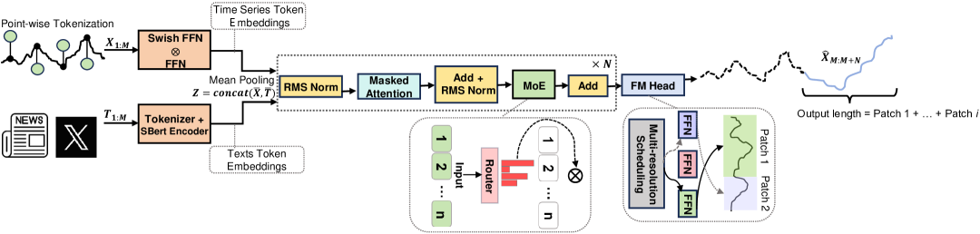
Figure 1: This figure presents the architecture of FTS-Text-MoE, a model designed to integrate textual and time series data for forecasting.

2 Related Works

Early studies on stock prediction using text analysis employed support vector machines (SVM) to extract basic features from text, such as bag-of-words, noun phrases, and named entities Schumaker and Chen (2009). These shallow features were later replaced by structured tuples (e.g., subject, action, object) extracted by deep neural networks Ding et al. (2015); Deng et al. (2019). Additionally, Xu and Cohen (2018) extracted implicit text vectors and used variational autoencoders (VAE) to model stock price prediction as a binary classification problem. As understanding of text complexity grew, Xu and Cohen (2018); Yang et al. (2020); Deng et al. (2019) began extracting richer implicit information from pre-trained text embeddings. Recent studies, such as Wang et al. (2025); Liu et al. (2025), used text as prompts to further enhance the accuracy of LLMs in time-series prediction. Unlike these methods, our research couples text sentences at each time point with corresponding time series data, predicting the next time series value, providing clearer analysis and exploring the specific impact of text on stock price fluctuations.

Sparse Deep Learning for Time Series. Deep learning models are typically large-scale and parameter-intensive Hoefler et al. (2021), requiring significant memory and computational resources. Sparse networks, such as MoE Jacobs et al. (1991), use dynamic routing to specialized experts, improving efficiency while maintaining or exceeding generalization performance Fedus et al. (2022). Traditional time series models, like DLinear Zeng et al. (2023) and SparseTSF Lin et al. (2024), are usually smaller and have less focus on sparse methods. After large-scale pretraining, studies such as MoLE Ni et al. (2024) and IME Ismail et al. explore sparsity but are not fully sparse models, as they route inputs to all attention heads before aggregation. The recent study Time-MoE Shi et al. (2024) uses sparse foundational models for general time-series forecasting but does not consider the impact of real-world textual information on numerical features. We further investigate whether complex textual information can enhance the interpretability of numerical predictions.

3 Methodology

We propose FTS-Text-MoE (Figure 1), a decoder-only Transformer architecture utilizing an MoE framework. The model comprises three components: (1) input token embedding, (2) MoE Transformer module, and (3) multi-resolution forecasting.

Problem Formulation.

Given historical numerical observations $\mathbf{X}_{1:M}=\left(x_{1},x_{2},\ldots,x_{M}\right)\in\mathbb{R}^{M}$ and corresponding textual data $\mathbf{T}_{1:M}=\left(t_{1},t_{2},\ldots,t_{M}\right)\in\mathbb{R}^{M}$ over the past $M$ days, our goal is to predict the next $N$ days: $\hat{\mathbf{X}}_{M+1:M+N}=f_{\theta}\left(\mathbf{X}_{1:M},\mathbf{T}_{1:M}\right)\in\mathbb{R}^{N}$ where $f_{\theta}$ represents the proposed model. FTS-Text-MoE supports flexible context lengths ($M$) and forecasting horizons ($N$) during inference, unlike traditional fixed-horizon models. Following the channel independence principle from Nie et al. , multivariate series are decomposed into univariate series, enabling better generalization across tasks.

3.1 Input Token Embedding

Text Token Embedding

We present an efficient pipeline for converting raw text into high-quality embeddings. On a daily basis, we select the top $k$ news articles and X Comments (Figure 2), embedding them using a pretrained DistilBART-12-6-cnn model. The resulting summaries are tokenized using the MiniLM L3 v2 (para) tokenizer and subsequently transformed into semantic representations using the SBertEncoder.

Time Token Embedding

Each time point in the financial time series is embedded using SwiGLU Shazeer (2020):

$$\mathbf{h}_{t}^{0}=\operatorname{SwiGLU}(x_{t})=\operatorname{Swish}(Wx_{t})\otimes(Vx_{t}),$$ (1)

where $W\in R^{D\times 1}$ and $V\in R^{D\times 1}$ and are learnable parameters, and denotes the hidden dimension.

Textual and numerical embeddings undergo mean pooling for aggregation before entering the subsequent MoE Transformer modules.

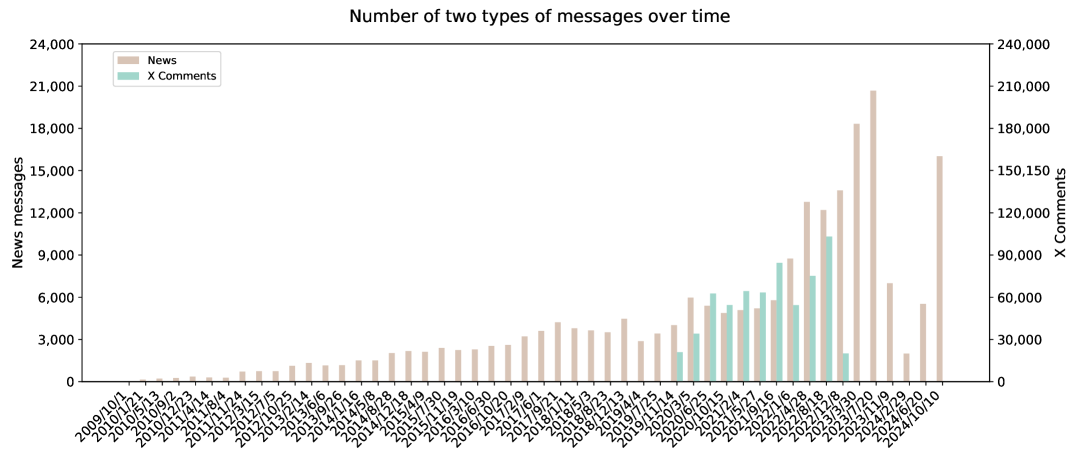
Figure 2: The x-axis represents dates, with each bar indicating the distribution of two text sources over the following 112 days.

Sector	Chronos		Moirai		$\text{Ours}_{\text{ts}}$		$\text{Ours}_{\text{ts\&news}}$		$\text{Ours}_{\text{ts\&x comments}}$
	MSE ($\downarrow$)	MAE ($\downarrow$)	MSE ($\downarrow$)	MAE ($\downarrow$)	MSE ($\downarrow$)	MAE ($\downarrow$)	MSE ($\downarrow$)	MAE ($\downarrow$)	MSE ($\downarrow$)	MAE ($\downarrow$)
Basic Materials	0.6458	0.8112	0.8725	0.8399	0.5540	0.6591	0.1972	0.3849	0.3866	0.5505
Financial Services	0.7247	0.7549	0.7466	0.7644	0.5498	0.6429	0.2060	0.3913	0.2077	0.3914
Consumer Defensive	0.1946	0.4503	0.1533	0.3558	0.5717	0.6721	0.5717	0.6721	0.5700	0.6710
Utilities	0.7518	0.9498	0.2517	0.4080	0.2797	0.4188	0.2797	0.4188	0.0527	0.1698
Energy	0.2094	0.3878	0.3204	0.4979	0.4196	0.5835	0.4196	0.5835	0.1392	0.3615
Technology	0.8681	0.8893	0.5858	0.5920	0.7480	0.7412	0.8688	0.8279	0.1538	0.3643
Consumer Cyclical	0.3628	0.5345	0.8673	0.9623	0.3116	0.5074	0.1632	0.3486	0.1049	0.2252
Real Estate	0.2282	0.4495	0.3687	0.4488	0.3567	0.5419	0.3892	0.5461	0.3550	0.5420
Healthcare	0.3521	0.4199	0.5786	0.6337	0.2248	0.4226	0.0705	0.2162	0.1299	0.3057
Communication Services	0.2029	0.3351	0.7599	0.8566	0.3388	0.5166	0.0511	0.1817	0.0697	0.2225
Industrials	0.4708	0.5574	0.2126	0.5158	0.1226	0.2743	0.5829	0.6761	0.1224	0.2741

Table 1: Analysis of FTS-Text-MoE Performance with Mixed Text Inputs vs. Baselines

3.2 FTS-Text-MoE Transformer

Inspired by Shi et al. (2024), we utilize a decoder-only Transformer Vaswani et al. (2017); Chen et al. (2024), incorporating advancements from LLMs Touvron et al. (2023). To enhance training stability, we apply RMSNorm Zhang and Sennrich (2019) at each sub-layer input. Rotary Positional Embeddings Su et al. (2024) improve sequence flexibility and extrapolation. Following Chowdhery et al. (2023), we eliminate most biases, retaining them only in the QKV layers of self-attention for better extrapolation. Formally, the architecture is defined as follows:

To introduce sparsity, we replace the standard FFN with a MoE layer, sharing a pool of sparsely activated experts. Each Mixture layer comprises multiple expert networks akin to standard FFNs, where each timestep routes inputs to either a single expert Fedus et al. (2022) or multiple experts Lepikhin et al. . One shared expert captures common knowledge across contexts. The Mixture function is defined as follows:

$$\operatorname{Mixture}(\bar{\mathbf{a}}_{t}^{l})=g_{N+1,t}\operatorname{FFN}_{N+1}(\bar{\mathbf{a}}_{t}^{l})+\sum_{i=1}^{N}g_{i,t}\operatorname{FFN}_{i}(\bar{\mathbf{a}}_{t}^{l})$$ (3)

$$\vskip-5.69054ptg_{i,t}=\begin{cases}s_{i,t},&\text{if }s_{i,t}\in\operatorname{TopK}\left(\{s_{j,t}\mid 1\leq j\leq N\},K\right),\\[3.0pt] 0,&\text{otherwise}.\end{cases}$$ (4)

$$\vskip-14.22636ptg_{N+1,t}=\operatorname{Sigmoid}(\mathbf{W}_{N+1}^{l}\bar{\mathbf{a}}_{t}^{l})$$ (5)

$$\vskip-5.69054pts_{i,t}=\operatorname{Softmax}_{i}(\mathbf{W}_{i}^{l}\bar{\mathbf{a}}_{t}^{l})$$ (6)

Here, ${W}_{i}^{l}\in{R}^{1\times D}$ are trainable parameters, $N$ is the number of non-shared experts, and $K$ denotes the activated non-shared experts per MoE layer.

FTS-Text-MoE boosts efficiency by activating only a subset of its 113M parameters, with just 50M active during operation. This selective activation enables the model to utilize specialized experts, boosting efficiency while preserving scalability.

3.3 Multi-resolution Prediction

Unlike existing foundational models, which typically output predictions at a fixed horizon, our model incorporates a multi-resolution prediction head followed by Shi et al. (2024). This prediction head consists of $P$ ($P=4$) output projections, each targeting a specific forecasting horizon $p_{j}\in\{1,8,32,64\}$, predicting $p_{j}$ future timesteps. During inference, we apply a greedy scheduling algorithm to concatenate these projections, enabling flexible, arbitrary-length forecasting and enhancing the adaptability of FTS-Text-MoE.

3.4 Loss Function

The multi-resolution prediction head comprises several single-layer FFN output projections, each dedicated to a specific forecasting horizon. The final loss combines autoregressive losses across multiple resolutions and an auxiliary balancing loss, as detailed in Appendix A.1:

$$\mathcal{L}= \frac{1}{P}\sum_{j=1}^{P}\mathcal{L}_{\text{ar}}(\mathbf{A}_{t+1:t+p_{j}},\hat{\mathbf{A}}_{t+1:t+p_{j}})$$ (7)

$$+\alpha\mathcal{L}_{\text{aux}},$$

Where $P$ denotes the number of multi-resolution projections, and $p_{j}$ represents the horizon length of the $j$-th projection. $\mathcal{L}{\text{ar}}$ (autoregressive loss) quantifies the difference between actual and predicted values to optimize prediction accuracy, while $\mathcal{L}{\text{aux}}$ (auxiliary loss) balances expert utilization, ensuring more even distribution and enhancing training efficiency.

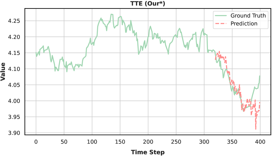
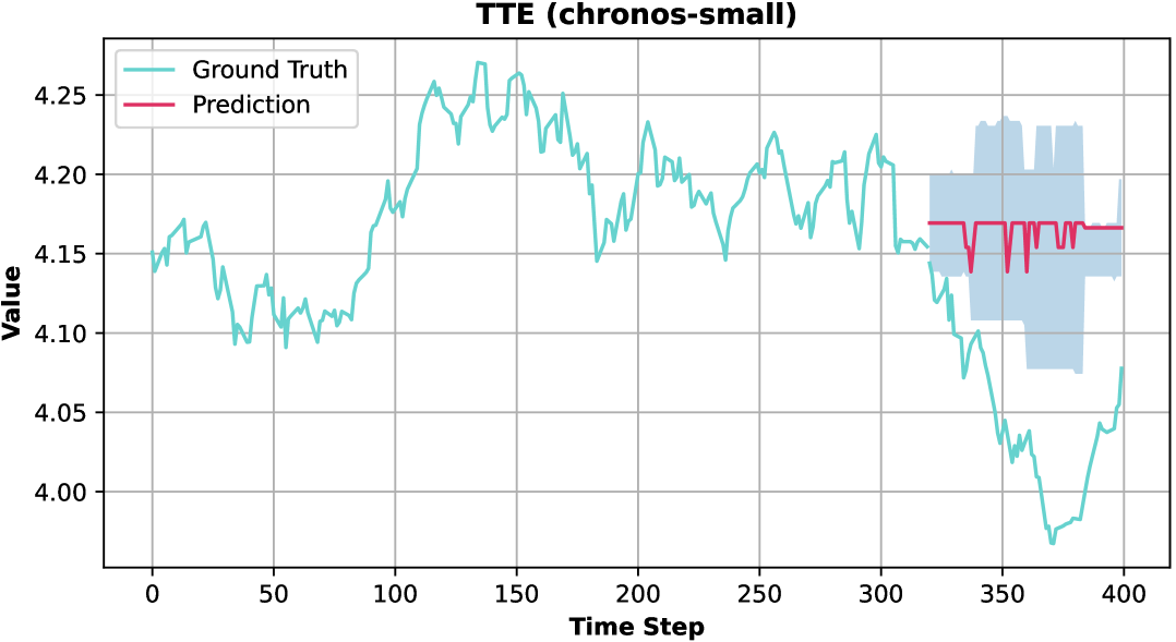
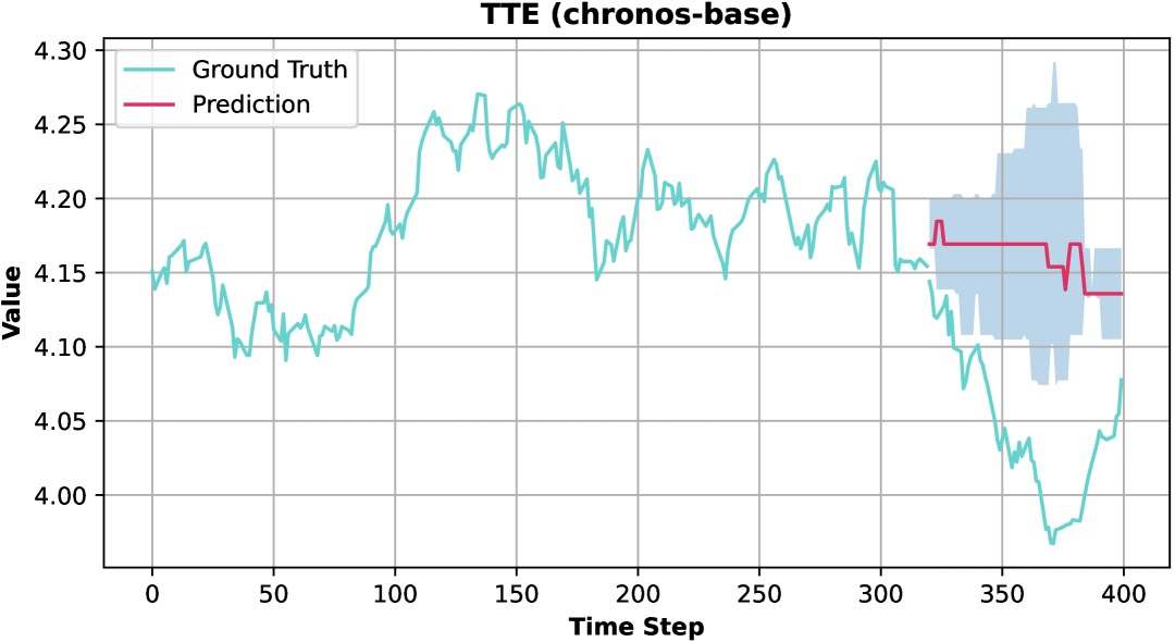
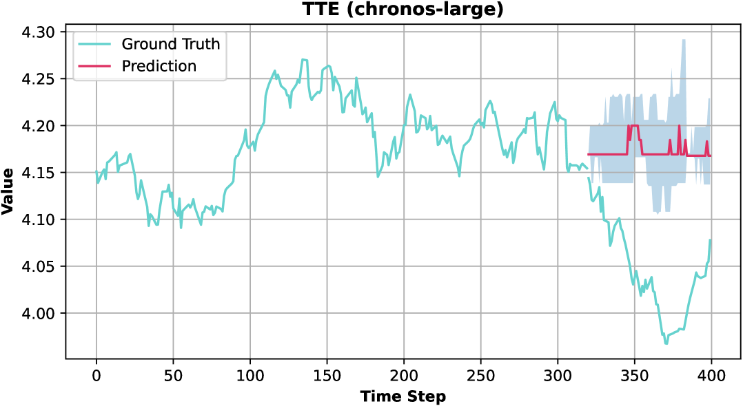
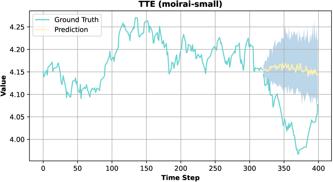
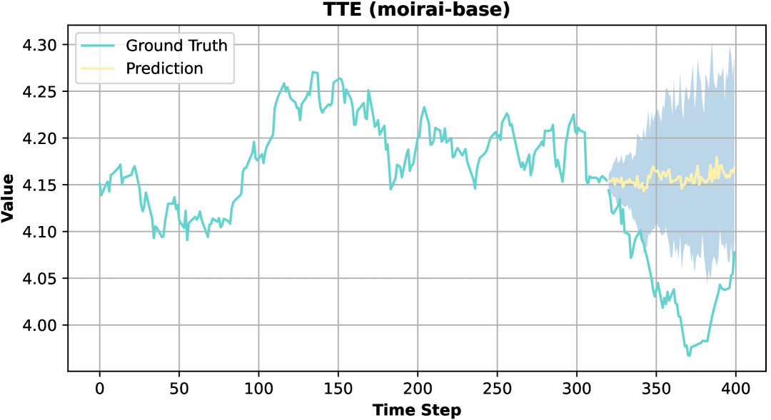
Figure 3: Forecasting results of different models on the TTE stock time series with a forecast horizon of 80 and a context length of 320. The green/blue lines represent the ground truth, while the red/yellow lines indicate the model predictions.

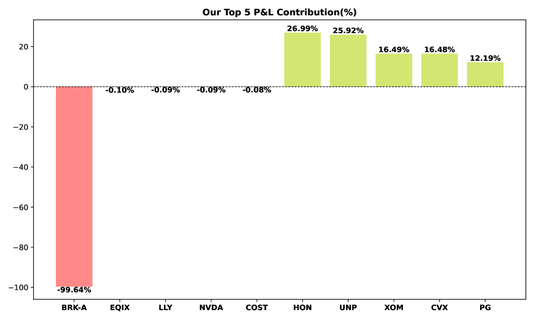
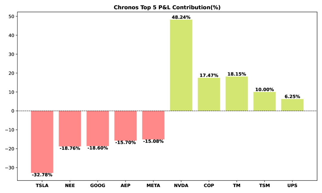
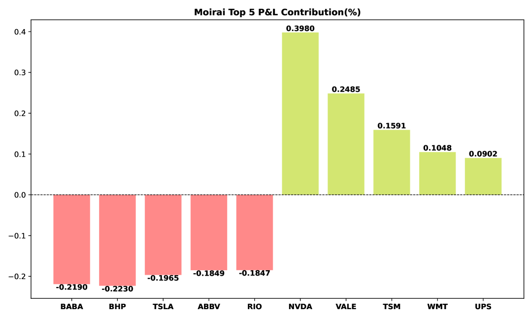
Figure 4: The top 5 gainers and losers under the three methods. The y-axis represents the proportion of contributions to returns and losses, while the x-axis denotes individual stock.

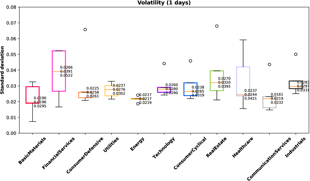
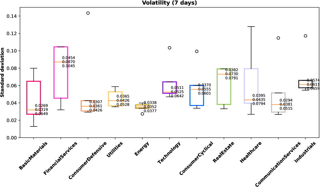
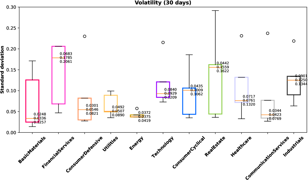
Figure 5: Stock price volatility across 11 industry sectors over 1-day, 7-day, and 30-day sampling periods.

4 Experiments

To evaluate the effectiveness of FTS-Text-MoE, we compared it with state-of-the-art language models designed for time series prediction. Details on datasets and metrics can be found in Appendix B.

4.1 Baselines

We use state-of-the-art models designed for long-term time series forecasting as baselines.

Chronos: Chronos Ansari et al. discretizes time series into intervals by scaling and quantizing real values. This enables training language models on the "language of time series" without altering the model architecture. We evaluate Chronos models (t5-small/base/large).

Moirai: Moirai Woo et al. (2024) concatenates multivariate time series into a single sequence with [MASK] tokens for prediction, and the model uses multi-granularity patching to handle different frequencies. We evaluate Moirai models (t5-small/base).

4.2 Performance Comparison

In this section, we quantitatively and qualitatively assess the predictive performance of our FTS-Text-MoE model against those baselines.

4.2.1 Effect of Text Source and Length on Prediction Accuracy

We compare performance using Mean Squared Error (MSE) and Mean Absolute Error (MAE) across 11 industry sectors, integrating stock time series data with various textual inputs—summarized news and summarized X comments. Lower MSE and MAE values indicate superior predictive accuracy.

Our analysis highlights that adding summarized news or tweet inputs significantly improves stock movement prediction accuracy (Table 1). Specifically, using summarized X comments results in consistently lower MSE and MAE compared to models using only news or other inputs. This indicates that distilled sentiment signals effectively reduce noise and enhance prediction accuracy. Industry-level analysis reveals that sectors like Healthcare, Consumer Cyclical, and Communication Services exhibit lower prediction errors, suggesting a strong reliance on textual signals and improved performance with text integration. In contrast, industries like Energy and Industrials, which experience higher volatility, show improved accuracy with textual inputs but still exhibit larger errors.

4.2.2 Prediction Performance of TS Models

When compared to the baseline models, Chronos and Moirai, FTS-Text-MoE shows improved performance with the addition of text inputs (such as news and tweets), but still falls short of surpassing Chronos and Moirai in some industries and scenarios (Table 1). Chronos and Moirai models exhibit a more conservative prediction approach, especially under high uncertainty and market volatility, smoothing the curve to reduce errors and maintain lower MSE and MAE. In contrast, FTS-Text-MoE adopts a more proactive strategy, capturing short-term volatility, which benefits quick market shifts but increases prediction errors during periods of significant fluctuations3.

Approach	Overall ($\uparrow$)	Std. Dev. ($\downarrow$)	Sharpe ($\uparrow$)
1/N	0.0570	5.132e-3	0.1725
S&P500 Index	-0.0082	5.459e-3	-0.3002
Moirai	0.0079	1.741e-3	0.3320
Chronos	-0.0077	1.288e-3	0.1223
Our	0.1347	5.290e-3	1.0818

Table 2: Performance comparison of different portfolio approaches. Overall, Std. Dev., and Sharpe can be referred to in Appendix B.7, formulas 14, 15 and 17.

4.3 Robustness Analysis of FTS-Text-MoE

We analyzed stock price volatility across sectors (see Figure 5), measuring it as the standard deviation of changes over a given sampling period ($P=1,7,30$): Higher volatility indicates greater risk, which generally increases with a longer sampling period $P$.

$$\sigma_{P}=\sqrt{\frac{1}{N_{P}}\sum_{i=d_{0}}^{d_{n}-P}(v_{i}^{P}-\overline{v_{P}})^{2}},$$ (8)

where $d_{0}$ and $d_{n}$ are the first and last days, $v_{i}^{P}=y_{i+P}-y_{i}$ represents the value change over $P$, and $\overline{v_{P}}$ is the average change:

$$\overline{v_{P}}=\frac{1}{N_{P}}\sum_{i=d_{0}}^{d_{n}-P}v_{i}^{P}.$$ (9)

4.4 Comparison of Return and Loss Distributions

Compared to FTS-Text-MoE, Chronos and Moirai, which rely solely on historical time-series data, adopt a more passive prediction strategy. In contrast, FTS-Text-MoE integrates real-world textual information, resulting in a more aggressive forecasting approach. Figure 4 shows the top five gainers and losers for FTS-Text-MoE and the baseline models. The return distribution for FTS-Text-MoE is noticeably more uneven, indicating a more aggressive and concentrated investment strategy.

4.5 Portfolio Optimization

We evaluate portfolio performance using three key metrics across four baselines:

• 1/N Portfolio: Equally weighted across 11 stocks.

• S&P 500 Index: Market benchmark.

• Moirai/Chronos Positive Prediction Portfolios: Invests only in positively predicted stocks, equally weighted.

As shown in Table 2, FTS-Text-MoE, following the same investment approach, outperforms Moirai/Chronos, particularly in terms of overall returns and Sharpe ratio. With an Overall return of 0.1347, it demonstrates superior cumulative returns, while its Sharpe ratio of 1.0818 indicates better risk-adjusted performance. However, its higher standard deviation (Std. Dev. = 5.290e-3) suggests increased return volatility, likely due to the model’s responsiveness to time series fluctuations, making it more sensitive to short-term market dynamics.

5 Conclusion

This study proposes FTS-Text-MoE, which effectively integrates time series and textual data to overcome the input-output length limitations faced by existing large-scale financial forecasting models when processing multi-source data and performing long-sequence predictions. The proposed model employs a sparse Transformer decoder combined with an MoE mechanism, significantly enhancing computational efficiency, and utilizes multi-resolution prediction heads to enable flexible forecasting across different temporal scales. Experimental results demonstrate that FTS-Text-MoE achieves superior performance in financial time series prediction tasks, effectively integrating quantitative and sentiment data for a more comprehensive market analysis.

6 Limitations

The proposed FTS-Text-MoE integrates financial numerical data with textual information and reduces computational complexity using a sparse Transformer decoder, but it has limitations. Firstly, the model aligns textual and time-series data at the same time step, yet news and tweets often have a delayed impact on stock prices. This lag, where market information takes time to propagate, may affect prediction accuracy. Secondly, news and social media may contain false or misleading information, negatively influencing forecasts. Future research will focus on handling lag and improving text authenticity verification to enhance model robustness and accuracy.

Appendix A Implementation Details

A.1 Loss Function

Integrating extensive textual information into financial time series data poses a challenge for training stability in FTS-Text-MoE. To enhance robustness against outliers and improve stability, we employ the Huber loss. The autoregressive loss, projected from a single-layer FFN, is defined as follows:

where $\delta$ is a hyperparameter that balances the L1 and L2 loss components.

In MoE architectures, optimizing purely for accuracy often leads to uneven expert utilization, with the model favoring a small subset of experts, limiting broader training. To address this, inspired by Dai et al. (2024) and Fedus et al. (2022), we introduce an auxiliary loss for expert load balancing. This loss aligns the proportion of tokens assigned to each expert ($f_{i}$) with its routing probability ($r_{i}$), ensuring a more balanced distribution.

$$\mathcal{L}_{\text{aux}}=N\sum_{i=1}^{N}f_{i}r_{i},\ r_{i}=\frac{1}{T}\sum_{t=1}^{T}s_{i,t},$$ (11)

$$f_{i}=\frac{1}{KT}\sum_{t=1}^{T}\mathbb{I}\Big{(}\text{Time step }t\text{ selects Expert }i\Big{)}$$

where $\mathbb{I}$ is an indicator function.

The multi-resolution forecasting heads utilize multiple output projections from a single-layer FFN, each corresponding to a different forecasting horizon. During training, errors across scales are aggregated into a composite loss. The final loss function combines the multi-resolution autoregressive loss and the auxiliary balancing loss:

$$\mathcal{L}=\frac{1}{P}\sum_{j=1}^{P}\mathcal{L}_{\text{ar}}\Big{(}\mathbf{A}_{t+1:t+p_{j}},\hat{\mathbf{A}}_{t+1:t+p_{j}}\Big{)}+\alpha\mathcal{L}_{\text{aux}},$$ (12)

where $P$ is the number of multi-resolution projections, and $p_{j}$ denotes the horizon of the $j$-th projection.

A.2 Model Details

FTS-Text-MoE employs a 12-layer architecture with 12 attention heads per layer and integrates an MoE module with 8 experts per layer. For each token, the top-2 experts ($K=2$) are selected. The model features a hidden dimension ($d_{\text{model}}$) of 384, a feed-forward network dimension ($d_{f}$) of 1536, and each expert has a dimension of 192 ($d_{\text{expert}}$). This design results in 50M active parameters during inference, with a total parameter count of 113M.

A.3 Training Configuration

Each model is trained for 10,000 steps with a batch size of 64 and a maximum sequence length of 1,024. Each iteration processes 64 time steps. The output projection employs prediction horizons of {1, 8, 32, 64}, and the auxiliary loss coefficient $\alpha$ is set to 0.02. Optimization is performed using the AdamW optimizer with hyperparameters: learning rate $lr=5\text{e-}5$, weight decay $\lambda=0.1$, $\beta_{1}=0.9$, and $\beta_{2}=0.95$. The learning rate follows a schedule with a linear warm-up for the first 10,000 steps, after which cosine annealing is applied. Training is conducted on two NVIDIA A6000-48G GPUs with FP16 precision. To improve batch efficiency and handle variable-length sequences, we employ sequence packing to minimize padding overhead.

Appendix B Data Sources and Metrics

B.1 Time Series Data

Stock price data from Yahoo Finance includes 55 stocks across 11 industries with daily open, high, low, close prices, and trading volume. The adjusted closing price is used as the primary measure of stock value over 20 years, yielding 191,512 sample points. See Table 3 for details.

Sector	Stock Symbol	Total Days	First Date	Last Date
Basic Materials	BHP	5568	2009/10/21	2025/1/17
	RIO	4461	2012/10/31	2025/1/16
	SHW	3390	2015/10/6	2025/1/15
	VALE	5465	2010/2/1	2025/1/17
	APD	4796	2011/12/2	2025/1/17
Financial Services	BRK-A	5570	2009/10/19	2025/1/18
	V	5392	2010/4/15	2025/1/19
	JPM	1840	2020/1/5	2025/1/17
	MA	1840	2020/1/5	2025/1/17
	BAC	1840	2020/1/5	2025/1/18
Consumer Defensive	WMT	2240	2018/12/1	2025/1/19
	PG	1840	2020/1/5	2025/1/18
	KO	5575	2009/10/14	2025/1/18
	PEP	5548	2009/11/10	2025/1/19
	COST	5449	2010/2/17	2025/1/18
Utilities	NEE	1639	2020/7/24	2025/1/17
	DUK	5381	2010/4/26	2025/1/17
	D	5387	2010/4/20	2025/1/18
	SO	5324	2010/6/22	2025/1/18
	AEP	5579	2009/10/9	2025/1/16
Energy	XOM	1973	2019/8/25	2025/1/18
	CVX	3090	2016/8/3	2025/1/18
	SHEL	1840	2020/1/5	2025/1/17
	TTE	1839	2020/1/5	2025/1/16
	COP	5541	2009/11/17	2025/1/17
Technology	AAPL	1844	2020/1/1	2025/1/18
	MSFT	1840	2020/1/5	2025/1/18
	TSM	5392	2010/4/15	2025/1/19
	NVDA	1615	2020/8/17	2025/1/20
	AVGO	1839	2020/1/6	2025/1/19
Consumer Cyclical	AMZN	1844	2020/1/1	2025/1/19
	TSLA	1841	2020/1/4	2025/1/19
	HD	1841	2020/1/4	2025/1/17
	BABA	3725	2014/11/7	2025/1/17
	TM	5465	2010/2/1	2025/1/18
Real Estate	AMT	5526	2009/12/2	2025/1/17
	PLD	5322	2010/6/24	2025/1/18
	CCI	5442	2010/2/23	2025/1/16
	EQIX	3469	2015/7/21	2025/1/17
	PSA	3286	2016/1/20	2025/1/17
Healthcare	UNH	1839	2020/1/6	2025/1/20
	JNJ	1836	2020/1/9	2025/1/18
	LLY	1840	2020/1/5	2025/1/18
	PFE	1839	2020/1/6	2025/1/18
	ABBV	4398	2013/1/3	2025/1/17
Communication Services	GOOG	2173	2019/2/6	2025/1/19
	META	1841	2020/1/4	2025/1/19
	VZ	1833	2020/1/12	2025/1/19
	CMCSA	2844	2017/4/6	2025/1/17
	DIS	2046	2019/6/13	2025/1/18
Industrials	UPS	5538	2009/11/20	2025/1/18
	UNP	5555	2009/11/3	2025/1/18
	HON	1837	2020/1/8	2025/1/18
	LMT	1841	2020/1/4	2025/1/18
	CAT	5554	2009/11/4	2025/1/17

Table 3: Stock Price Series: Collection Periods and Total Days by Sector

B.2 Tweet Data

Given the vast number of daily tweets, we use a dataset clustered via the BERTopic pipeline. It includes tweets about the top 5 stocks in 11 sectors from 2020 to 2022, collected via the Twitter API. The dataset comprises 637,395 tweets. See Table 4 for details.

Company	Total Days	Daily Tweet Count	First Date	Last Date
AAPL	1090	83964	2020/1/1	2022/12/31
ABBV	914	3200	2020/1/4	2022/12/21
AEP	416	2156	2020/1/12	2022/12/28
AMT	546	2536	2020/1/10	2022/12/24
AMZN	1090	58193	2020/1/1	2022/12/31
APD	444	2283	2020/1/4	2022/12/16
AVGO	776	2466	2020/1/6	2022/12/24
BABA	978	18761	2020/1/4	2022/12/24
BAC	1046	7353	2020/1/5	2022/12/24
BHP	446	1433	2020/1/7	2022/12/23
BRK-A	414	1910	2020/1/4	2022/12/29
CAT	937	4823	2020/1/6	2022/12/24
CCI	339	1651	2020/1/5	2022/12/24
CMCSA	806	2412	2020/1/6	2022/12/24
COP	689	2027	2020/1/19	2022/12/24
COST	1003	4780	2020/1/7	2022/12/24
CVX	824	6907	2020/1/5	2022/12/24
D	462	1353	2020/1/12	2022/12/24
DIS	1064	14146	2020/1/8	2022/12/24
DUK	357	1688	2020/1/9	2022/12/24
EQIX	441	2505	2020/1/5	2022/12/28
GOOG	1085	12539	2020/1/4	2022/12/24
HD	923	4837	2020/1/4	2022/12/24
HON	464	1436	2020/1/8	2022/12/24
JNJ	884	6104	2020/1/9	2022/12/20
JPM	950	7783	2020/1/5	2022/12/24
KO	828	3915	2020/1/7	2022/12/24
LLY	745	2781	2020/1/5	2022/12/24
LMT	733	2620	2020/1/4	2022/10/17
MA	913	3408	2020/1/5	2022/12/24
META	965	44182	2020/1/4	2022/12/24
MSFT	963	31153	2020/1/4	2022/12/24
NEE	559	1637	2020/1/4	2022/12/24
PEP	669	2196	2020/1/15	2022/12/24
PFE	1031	12021	2020/1/6	2022/12/24
PG	727	2665	2020/1/5	2022/12/24
PLD	505	2362	2020/1/9	2022/12/24
PSA	499	2482	2020/1/11	2022/12/27
RIO	578	2005	2020/1/6	2022/12/24
SHEL	406	1688	2020/1/5	2022/12/23
SHW	398	1939	2020/1/4	2022/12/23
SO	365	1590	2020/1/4	2022/12/29
TM	560	2053	2020/1/5	2022/12/23
TSLA	973	181368	2020/1/4	2022/12/24
TSM	786	3850	2020/1/6	2022/12/24
TTE	404	1911	2020/1/5	2022/12/24
UNH	818	2550	2020/1/6	2022/12/24
UNP	398	1557	2020/1/4	2022/12/22
UPS	803	2805	2020/1/4	2022/12/23
V	936	5293	2020/1/4	2022/12/24
VALE	660	1937	2020/1/4	2022/12/24
VZ	745	3119	2020/1/12	2022/12/24
WMT	1076	11164	2020/1/4	2022/12/24
XOM	1060	7933	2020/1/5	2022/12/24
NVDA	1074	33965	2020/1/4	2022/12/24

Table 4: Stock Tweets: Collection Periods and Total Days by Sector.

B.3 News Data

We extract news data from the FNSPID dataset, focusing on articles related to 55 S&P 500 stocks listed on NASDAQ from 1999 to 2023. This dataset includes URLs, headlines, and full news texts.

To ensure up-to-date coverage, we addressed technical issues in the FNSPID project, like automating page navigation, filtering pop-ups, and recognizing new web elements. Using Selenium, we retrieved news headlines and full content from NASDAQ. This update extends coverage to January 19, 2025, compiling 216,308 high-quality news records. See Table 5 for details.

Company	Total Days	Daily News Count	First Date	Last Date
AAPL	595	9365	2022/6/3	2025/1/18
ABBV	2669	6198	2013/1/3	2025/1/17
AEP	1224	1945	2009/10/9	2025/1/16
AMT	2196	6532	2009/12/2	2025/1/17
AMZN	307	5282	2023/3/9	2025/1/19
APD	1410	2213	2011/12/2	2025/1/17
AVGO	61	507	2023/12/16	2025/1/19
BABA	2573	9262	2014/11/7	2025/1/17
BHP	2354	4810	2009/10/21	2025/1/17
BRK	2087	9288	2009/10/19	2025/1/18
CAT	2366	5685	2009/11/4	2025/1/17
CCI	1156	1676	2010/2/23	2025/1/16
CMCSA	1877	4762	2017/4/6	2025/1/17
COP	2702	5711	2009/11/17	2025/1/17
COST	2883	7281	2010/2/17	2025/1/18
CVX	2217	9188	2016/8/3	2025/1/18
D	1691	2936	2010/4/20	2025/1/18
DIS	1667	9211	2019/6/13	2025/1/18
DUK	1925	3202	2010/4/26	2025/1/17
GOOG	1742	9226	2019/2/6	2025/1/19
KO	3143	8140	2009/10/14	2025/1/18
LLY	87	507	2023/12/16	2025/1/18
LMT	131	507	2023/12/15	2025/1/18
MSFT	631	9237	2022/4/26	2025/1/18
NEE	2383	4993	2010/7/24	2025/1/17
NVDA	828	9216	2021/8/17	2025/1/20
PEP	2519	5462	2009/11/10	2025/1/19
PLD	1434	2152	2010/6/24	2025/1/18
RIO	238	436	2012/10/31	2025/1/16
SHW	798	1218	2015/10/6	2025/1/15
SO	1577	2534	2010/6/22	2025/1/18
TM	2420	4083	2010/2/1	2025/1/18
TSLA	626	9212	2022/5/2	2025/1/19
TSM	2079	4398	2010/4/15	2025/1/19
UNP	1821	3084	2009/11/3	2025/1/18
UPS	2177	4217	2009/11/20	2025/1/18
V	2949	7445	2010/4/15	2025/1/19
VALE	1431	2015	2010/2/1	2025/1/17
WMT	1753	9154	2018/12/1	2025/1/19
XOM	1440	7253	2019/8/25	2025/1/18
BAC	96	500	2024/10/9	2025/1/18
EQIX	188	324	2015/7/21	2025/1/17
HD	146	500	2024/8/19	2025/1/17
HON	188	500	2024/5/14	2025/1/18
JNJ	127	500	2024/8/30	2025/1/18
JPM	89	500	2024/10/15	2025/1/17
MA	152	500	2024/8/1	2025/1/17
META	45	500	2024/12/6	2025/1/19
PFE	57	500	2024/10/18	2025/1/18
PG	182	500	2024/6/25	2025/1/18
PSA	146	241	2016/1/20	2025/1/17
SHEL	230	482	2024/2/1	2025/1/17
TTE	143	218	2024/2/13	2025/1/16
UNH	120	500	2024/9/5	2025/1/20
VZ	139	500	2024/8/21	2025/1/19

Table 5: Stock News: Collection Periods and Total Days by Sector.

B.4 Multimodal Data Alignment

To enhance stock prediction accuracy, we align time-stamped tweets, news articles, and stock prices as multimodal inputs. Integrating textual and numerical data improves predictive performance. For a comparison of daily tweet and news volumes, see Figure 2.

B.5 Text-Cleaning Pipeline

Earlier sections detailed dataset attributes, including sampling frequency, time series count, and total observations. Here, we provide the text-cleaning pipeline, which ranks raw text and extracts summaries (see Algorithms 1 and 2) before converting them into embeddings (see Algorithm 3). Tweets, being short, are not summarized.

Algorithm 1 News Ranking & Summarization

1:Input: $\mathcal{D}_{\text{raw}}$ (JSONLs with $\{$Date, Text$\}$)

2:Output: $\mathcal{D}_{\text{final}}$ (Summarized JSONLs)

3:Load pretrained tokenizer and summarization model

4:for each file in $\mathcal{D}_{\text{raw}}$ do

5:  Extract $c$ (company code) from filename

6:  Read JSONL and group records by $t$ (date)

7:  for each $t$ do

8:   Compute $\text{score}(x,c)$ for each $x$

9:   Select $x^{*}=\arg\max_{x}\text{score}(x,c)$

10:  end for

11:  Store $\mathcal{D}_{\text{ranked}}$

12:end for

13:for each file in $\mathcal{D}_{\text{ranked}}$ do

14:  for each $x\in\mathcal{D}_{\text{ranked}}$ do

15:   Truncate $x$ to $L_{\text{max}}=1024$

16:   Generate summary $\hat{x}$ using the pretrained model

17:   Store $\hat{x}$

18:  end for

19:end for

20:Return $\mathcal{D}_{\text{final}}$

Algorithm 2 X Comment Ranking

1:Input: $\mathcal{D}_{\text{raw}}$ (JSONLs with $\{$Date, Text$\}$)

2:Output: $\mathcal{D}_{\text{ranked}}$ (Ranked JSONLs)

3:for each file in $\mathcal{D}_{\text{raw}}$ do

4:  Extract company code $c$ from filename

5:  Read JSONL, group records by date $t$

6:  for each $t$ do

7:   Compute relevance score $\text{score}(x,c)$ for each $x$

8:   Select $x^{*}=\arg\max_{x}\text{score}(x,c)$

9:  end for

10:  Store $\mathcal{D}_{\text{ranked}}$

11:end for

12:Return $\mathcal{D}_{\text{ranked}}$

Algorithm 3 Text Embedding Generation

1:Input: $\mathcal{D}_{\text{ranked}}$ (JSONLs with $\{$Date, Text$\}$)

2:Output: $\mathcal{D}_{\text{emb}}$ (Embedded JSONLs)

3:Load pretrained tokenizer and encoder

4:Set device and batch size

5:for each file in $\mathcal{D}_{\text{ranked}}$ do

6:  Read JSONL, extract and clean text

7:  Tokenize and batch non-empty entries

8:  for each batch do

9:   Compute embeddings via pretrained model

10:  end for

11:  Replace text with embeddings, store $\mathcal{D}_{\text{emb}}$

12:end for

13:Return $\mathcal{D}_{\text{emb}}$

B.6 Input-Output Flow in FTS-Text-MoE for Time Series Forecasting

Figure 6 illustrates the input and output structure in time series forecasting using FTS-Text-MoE.

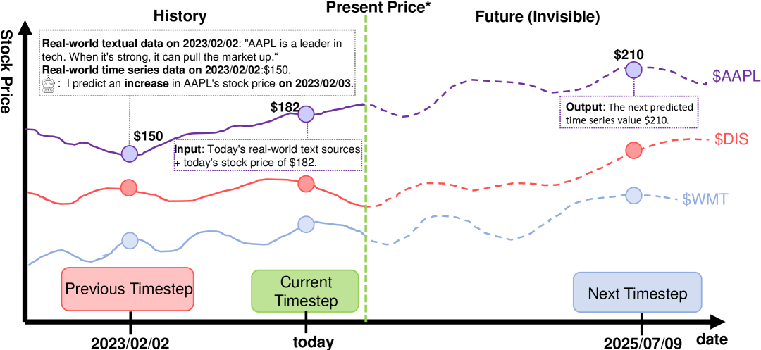
Figure 6: Illustration of Input and Output in Time Series Forecasting: FTS-Text-MoE takes the textual data and stock price of the current day as inputs and outputs the predicted stock price for the next day.

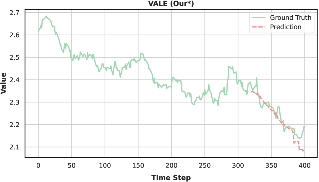
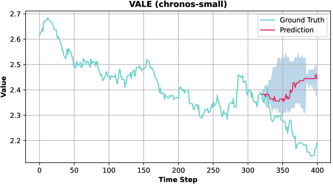
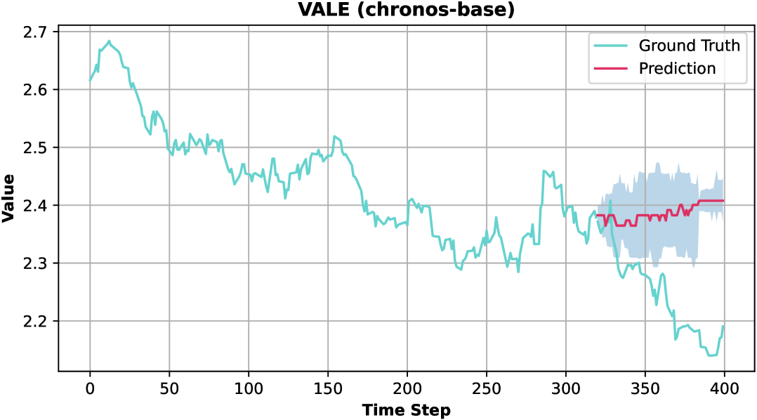
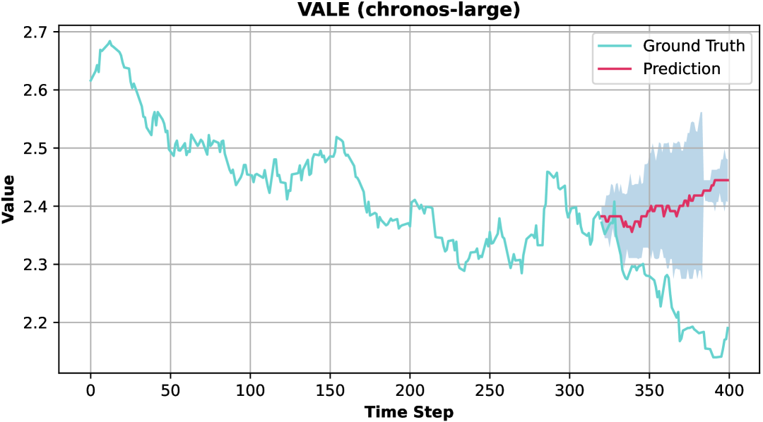
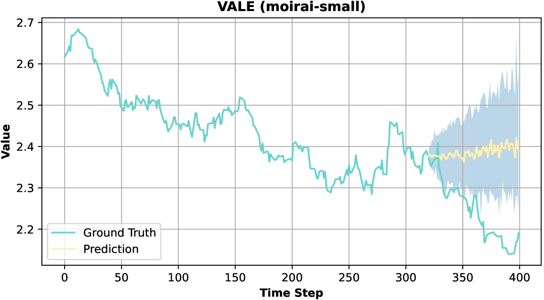
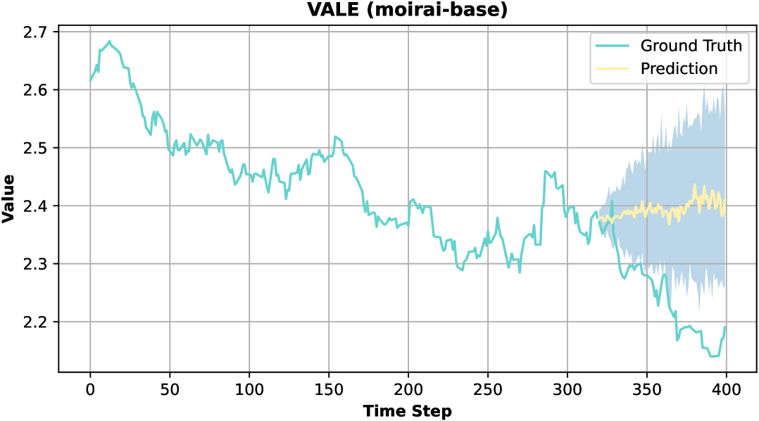
Figure 7: Forecasting results of different models on the VALE stock time series with a forecast horizon of 80 and a context length of 320. The green/blue lines represent the ground truth, while the red/yellow lines indicate the model predictions.

B.7 Evaluation Metrics

Error Metrics (Negative).

Model performance is evaluated using mean square error (MSE) and mean absolute error (MAE):

MSE $$=\frac{1}{H}\sum_{i=1}^{H}(x_{i}-\widehat{x}_{i})^{2},$$

MAE $$=\frac{1}{H}\sum_{i=1}^{H}|x_{i}-\widehat{x}_{i}|,$$ (13)

where $x_{i},\widehat{x}_{i}\in\mathbb{R}$ denote the ground truth and predicted values at time step $i$.

Overall (Positive).

Cumulative daily returns:

$$\text{Overall}=\sum_{i=1}^{n}R_{i}.$$ (14)

Std. Dev. (Negative).

Standard deviation of returns, indicating risk:

$$\sigma=\sqrt{\frac{1}{n-1}\sum_{i=1}^{n}\left(R_{i}-\bar{R}\right)^{2}},$$ (15)

where the mean return is:

$$\bar{R}=\frac{1}{n}\sum_{i=1}^{n}R_{i}.$$ (16)

Sharpe Lo (2002) (Positive).

Risk-adjusted return:

$$\text{Sharpe}=\frac{\bar{R}_{p}-R_{f}}{\sigma_{p}}\times\sqrt{252}.$$ (17)

where $\bar{R}_{p}$ is the portfolio’s average return, $R_{f}$ the risk-free rate, $\sigma_{p}$ the return standard deviation, and 252 the annualization factor.

These metrics provide a comprehensive evaluation of predictive accuracy and financial performance.

Appendix C Analysis of Financial Time-Series Results

As shown in Figure 7 (TTE stock time series data), Chronos and Moirai adopt a more conservative forecasting approach, with Moirai exhibiting the smoothest prediction curve. This suggests that Moirai prioritizes stability in high-uncertainty scenarios. In contrast, FTS-Text-MoE takes a more proactive approach, aiming to capture short-term fluctuations and better align with time series trends.

References

- (1) Abdul Fatir Ansari, Lorenzo Stella, Ali Caner Turkmen, Xiyuan Zhang, Pedro Mercado, Huibin Shen, Oleksandr Shchur, Syama Sundar Rangapuram, Sebastian Pineda Arango, Shubham Kapoor, and 1 others. Chronos: Learning the language of time series. Transactions on Machine Learning Research.
- Ariyo et al. (2014) Adebiyi A Ariyo, Adewumi O Adewumi, and Charles K Ayo. 2014. Stock price prediction using the arima model. In 2014 UKSim-AMSS 16th international conference on computer modelling and simulation, pages 106–112. IEEE.
- Chen et al. (2024) Jiayu Chen, Bhargav Ganguly, Yang Xu, Yongsheng Mei, Tian Lan, and Vaneet Aggarwal. 2024. Deep generative models for offline policy learning: Tutorial, survey, and perspectives on future directions. Transactions on Machine Learning Research.
- (4) Junyan Cheng and Peter Chin. Sociodojo: Building lifelong analytical agents with real-world text and time series. In The Twelfth International Conference on Learning Representations.
- Chowdhery et al. (2023) Aakanksha Chowdhery, Sharan Narang, Jacob Devlin, Maarten Bosma, Gaurav Mishra, Adam Roberts, Paul Barham, Hyung Won Chung, Charles Sutton, Sebastian Gehrmann, and 1 others. 2023. Palm: Scaling language modeling with pathways. Journal of Machine Learning Research, 24(240):1–113.
- Dai et al. (2024) Damai Dai, Chengqi Deng, Chenggang Zhao, RX Xu, Huazuo Gao, Deli Chen, Jiashi Li, Wangding Zeng, Xingkai Yu, and 1 others. 2024. Deepseekmoe: Towards ultimate expert specialization in mixture-of-experts language models. arXiv preprint arXiv:2401.06066.
- Deng et al. (2019) Shumin Deng, Ningyu Zhang, Wen Zhang, Jiaoyan Chen, Jeff Z Pan, and Huajun Chen. 2019. Knowledge-driven stock trend prediction and explanation via temporal convolutional network. In Companion proceedings of the 2019 world wide web conference, pages 678–685.
- Ding et al. (2015) Xiao Ding, Yue Zhang, Ting Liu, and Junwen Duan. 2015. Deep learning for event-driven stock prediction. In Proceedings of the 24th International Conference on Artificial Intelligence, pages 2327–2333.
- Fedus et al. (2022) William Fedus, Barret Zoph, and Noam Shazeer. 2022. Switch transformers: Scaling to trillion parameter models with simple and efficient sparsity. Journal of Machine Learning Research, 23(120):1–39.
- Francq and Zakoian (2019) Christian Francq and Jean-Michel Zakoian. 2019. GARCH models: structure, statistical inference and financial applications. John Wiley & Sons.
- Hoefler et al. (2021) Torsten Hoefler, Dan Alistarh, Tal Ben-Nun, Nikoli Dryden, and Alexandra Peste. 2021. Sparsity in deep learning: Pruning and growth for efficient inference and training in neural networks. Journal of Machine Learning Research, 22(241):1–124.
- Hsu et al. (2021) Yen-Ju Hsu, Yang-Cheng Lu, and J Jimmy Yang. 2021. News sentiment and stock market volatility. Review of Quantitative Finance and Accounting, 57(3):1093–1122.
- (13) Aya Abdelsalam Ismail, Sercan O Arik, Jinsung Yoon, Ankur Taly, Soheil Feizi, and Tomas Pfister. Interpretable mixture of experts. Transactions on Machine Learning Research.
- Jacobs et al. (1991) Robert A Jacobs, Michael I Jordan, Steven J Nowlan, and Geoffrey E Hinton. 1991. Adaptive mixtures of local experts. Neural computation, 3(1):79–87.
- Koa et al. (2023) Kelvin JL Koa, Yunshan Ma, Ritchie Ng, and Tat-Seng Chua. 2023. Diffusion variational autoencoder for tackling stochasticity in multi-step regression stock price prediction. In Proceedings of the 32nd ACM International Conference on Information and Knowledge Management, pages 1087–1096.
- Koa et al. (2024) Kelvin JL Koa, Yunshan Ma, Ritchie Ng, and Tat-Seng Chua. 2024. Learning to generate explainable stock predictions using self-reflective large language models. In Proceedings of the ACM Web Conference 2024, pages 4304–4315.
- Konstantinov et al. (2020) Gueorgui Konstantinov, Andreas Chorus, and Jonas Rebmann. 2020. A network and machine learning approach to factor, asset, and blended allocation. Journal of Portfolio Management, 46(6):54–71.
- Kumar et al. (2024) Pulikandala Nithish Kumar, Nneka Umeorah, and Alex Alochukwu. 2024. Dynamic graph neural networks for enhanced volatility prediction in financial markets. arXiv preprint arXiv:2410.16858.
- (19) Dmitry Lepikhin, HyoukJoong Lee, Yuanzhong Xu, Dehao Chen, Orhan Firat, Yanping Huang, Maxim Krikun, Noam Shazeer, and Zhifeng Chen. Gshard: Scaling giant models with conditional computation and automatic sharding. In International Conference on Learning Representations.
- Lin et al. (2024) Shengsheng Lin, Weiwei Lin, Wentai Wu, Haojun Chen, and Junjie Yang. 2024. Sparsetsf: Modeling long-term time series forecasting with* 1k* parameters. In International Conference on Machine Learning, pages 30211–30226. PMLR.
- Liu et al. (2025) Chenxi Liu, Qianxiong Xu, Hao Miao, Sun Yang, Lingzheng Zhang, Cheng Long, Ziyue Li, and Rui Zhao. 2025. Timecma: Towards llm-empowered multivariate time series forecasting via cross-modality alignment. In Proceedings of the AAAI Conference on Artificial Intelligence, volume 39, pages 18780–18788.
- Lo (2002) Andrew W Lo. 2002. The statistics of sharpe ratios. Financial analysts journal, 58(4):36–52.
- Montgomery et al. (2021) Douglas C Montgomery, Elizabeth A Peck, and G Geoffrey Vining. 2021. Introduction to linear regression analysis. John Wiley & Sons.
- Ni et al. (2024) Ronghao Ni, Zinan Lin, Shuaiqi Wang, and Giulia Fanti. 2024. Mixture-of-linear-experts for long-term time series forecasting. In International Conference on Artificial Intelligence and Statistics, pages 4672–4680. PMLR.
- (25) Yuqi Nie, Nam H Nguyen, Phanwadee Sinthong, and Jayant Kalagnanam. A time series is worth 64 words: Long-term forecasting with transformers. In The Eleventh International Conference on Learning Representations.
- Schumaker and Chen (2009) Robert P Schumaker and Hsinchun Chen. 2009. Textual analysis of stock market prediction using breaking financial news: The azfin text system. ACM Transactions on Information Systems (TOIS), 27(2):1–19.
- Shazeer (2020) Noam Shazeer. 2020. Glu variants improve transformer. arXiv e-prints, pages arXiv–2002.
- Shi et al. (2024) Xiaoming Shi, Shiyu Wang, Yuqi Nie, Dianqi Li, Zhou Ye, Qingsong Wen, and Ming Jin. 2024. Time-moe: Billion-scale time series foundation models with mixture of experts. arXiv preprint arXiv:2409.16040.
- Su et al. (2024) Jianlin Su, Murtadha Ahmed, Yu Lu, Shengfeng Pan, Wen Bo, and Yunfeng Liu. 2024. Roformer: Enhanced transformer with rotary position embedding. Neurocomputing, 568:127063.
- Touvron et al. (2023) Hugo Touvron, Thibaut Lavril, Gautier Izacard, Xavier Martinet, Marie-Anne Lachaux, Timothée Lacroix, Baptiste Rozière, Naman Goyal, Eric Hambro, Faisal Azhar, and 1 others. 2023. Llama: Open and efficient foundation language models. arXiv preprint arXiv:2302.13971.
- Vaswani et al. (2017) Ashish Vaswani, Noam Shazeer, Niki Parmar, Jakob Uszkoreit, Llion Jones, Aidan N Gomez, Łukasz Kaiser, and Illia Polosukhin. 2017. Attention is all you need. Advances in neural information processing systems, 30.
- Wang et al. (2025) Chengsen Wang, Qi Qi, Jingyu Wang, Haifeng Sun, Zirui Zhuang, Jinming Wu, Lei Zhang, and Jianxin Liao. 2025. Chattime: A unified multimodal time series foundation model bridging numerical and textual data. In Proceedings of the AAAI Conference on Artificial Intelligence, volume 39, pages 12694–12702.
- Woo et al. (2024) Gerald Woo, Chenghao Liu, Akshat Kumar, Caiming Xiong, Silvio Savarese, and Doyen Sahoo. 2024. Unified training of universal time series forecasting transformers. In Proceedings of the 41st International Conference on Machine Learning, pages 53140–53164.
- Xu and Cohen (2018) Yumo Xu and Shay B Cohen. 2018. Stock movement prediction from tweets and historical prices. In Proceedings of the 56th Annual Meeting of the Association for Computational Linguistics (Volume 1: Long Papers), pages 1970–1979.
- Yang et al. (2020) Linyi Yang, Tin Lok James Ng, Barry Smyth, and Riuhai Dong. 2020. Html: Hierarchical transformer-based multi-task learning for volatility prediction. In Proceedings of The Web Conference 2020, pages 441–451.
- Zeng et al. (2023) Ailing Zeng, Muxi Chen, Lei Zhang, and Qiang Xu. 2023. Are transformers effective for time series forecasting? In Proceedings of the AAAI conference on artificial intelligence, volume 37, pages 11121–11128.
- Zhang and Sennrich (2019) Biao Zhang and Rico Sennrich. 2019. Root mean square layer normalization. Advances in Neural Information Processing Systems, 32.