Development of a Chip-Scale Optical Gyroscope with Weak Measurement Amplification Readout
Abstract
The design of an integrated optical chip is proposed containing a rotation sensing ring resonator (optical gyroscope) coupled to an inverse weak value amplified Sagnac interferometer that amplifies the signal containing the phase information. We show that, for conservative parameter choices, our setup has a minimum detectable angular rotation rate hr and an Allan deviation hr under expected ideal conditions. We also show that for an appropriate amount of input power, our design can improve the signal-to-noise ratio, the precision of angular rotation rate, and error in detection by more than ten times compared to a Sagnac interferometer coupled to a ring resonator.
I Introduction
Inertial rotation sensors have a variety of applications ranging from inertial navigation systems used in aircrafts to geophysical applications such as determination of astronomical latitudeEzekiel and Arditty (1982). Although mechanical gyroscopes were used as rotation sensors in the past, they have had disadvantages such as the presence of moving parts, warm up time and g-sensitivityEzekiel and Arditty (1982); Venediktov et al. (2016). The advent of the laser allowed ring resonators to be used as purely optical gyroscopes that do not contain the aforementioned disadvantages of mechanical gyroscopesChow et al. (1985); Loukianov (1999). This is all thanks to the Sagnac effect that changes the optical length of the clockwise and counterclockwise paths around the ring such that they are not equal anymorePost (1967); Ezekiel and Arditty (1982); S. Ezekiel (1977); Meyer et al. (1983); Sagnac (1913).
Weak value amplification (WVA) can amplify small parameters while suppressing certain technical noises such that the system yields an increased signal-to-noise ratio (SNR) and shot noise limited sensitivityFeizpour et al. (2011); Song et al. (2021); Steinmetz et al. (2022); Lyons et al. (2018); Steinmetz et al. (2019). WVA consists of three steps: (i) pre-selection of the initial state of the system, (ii) a weak perturbation to the system state, and (iii) post-selection of the final state of the system, which is nearly orthogonal to the initial stateAharonov et al. (1988); Steinmetz et al. (2022, 2019). Technical advantages of WVA were discussed in detail in Refs.Jordan et al. (2014); Dixon et al. (2009).
In this paper, we discuss an integrated optical chip on which an optical ring resonator is coupled to an inverse weak value amplified (IWVA) Sagnac interferometer, which contains phase front tilters, a multi-mode directional coupler, and a multi-mode interferometer at the readout, as discussed in Refs.Steinmetz et al. (2022, 2019); Song et al. (2021). While the optical ring resonator functions as an optical gyroscope that provides a phase shift due to rotation of the ring explained by the Sagnac effect, the IWVA Sagnac interferometer inverse weak value amplifies (IWVA), discussed below, the phase shift through phase front tilting. A minimum detectable angular velocity of the order of hr is a key challenge for miniaturized gyroscopes and motivates the research efforts in the fieldDell’Olio et al. (2014). We show that, because of IWVA, our setup has a minimum detectable angular rotation rate hr under expected ideal conditions and improves the SNR and phase resolution compared to a common Sagnac interferometer. It is worth distinguishing WVA and IWVA in the context of this work. WVA is used in measuring the spatial phase front tilt by using known phase shiftSong et al. (2021); Hosten and Kwiat (2008). On the other hand, IWVA, which is the method used in this paper, is used in measuring the phase shift with amplified signal by using the known spatial phase front tiltSong et al. (2021); Starling et al. (2010).
The paper is organized as follows: in Sec. II, we discuss the setup of our system, including the 50/50 beam splitter, the coupling between IWVA Sagnac interferometer and the optical ring, and the phase and amplitude amplification of the electric field coming out of the optical ring. In Sec. III, we discuss the 50/50 beam splitter before the output and derive the signal-to-noise ratio (SNR), phase resolution, and Allan deviation for two different systems: (i) a common Sagnac interferometer coupled to an optical ring and (ii) IWVA Sagnac interferometer coupled to an optical ring. We then compare the two systems and discuss the advantages of using IWVA Sagnac over common Sagnac interferometer. Finally, in Sec. IV, we conclude our results.
II The System
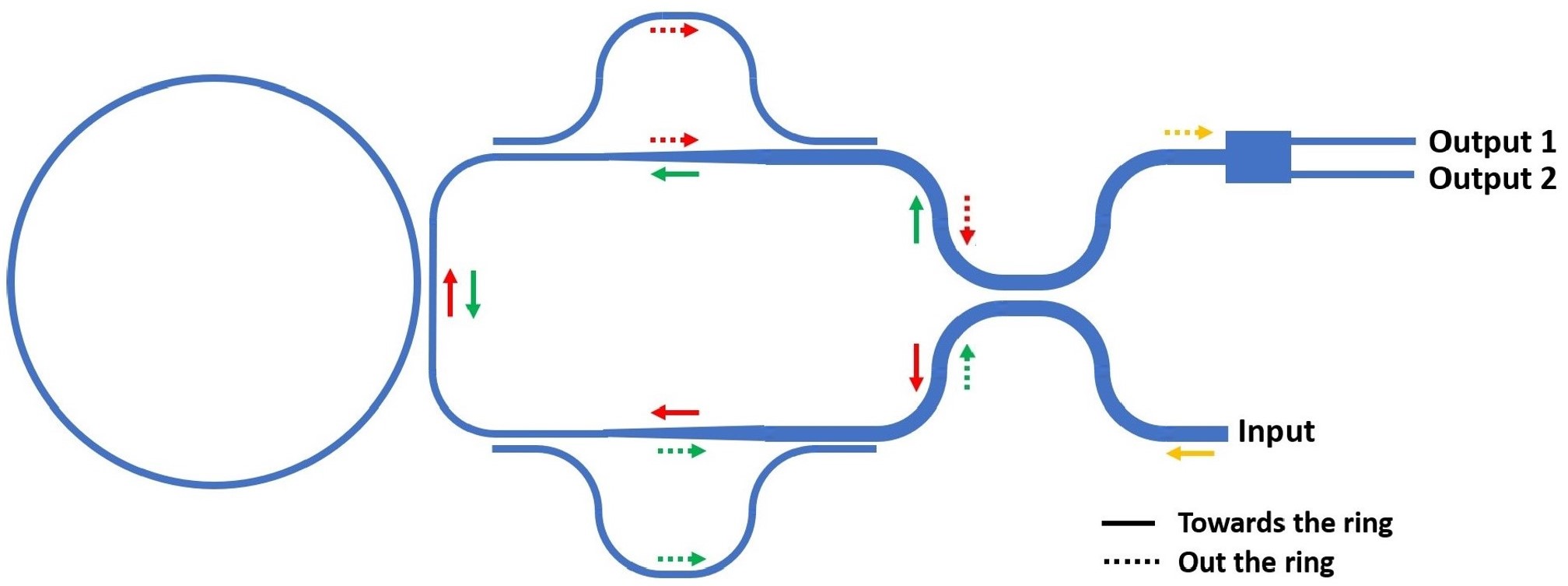
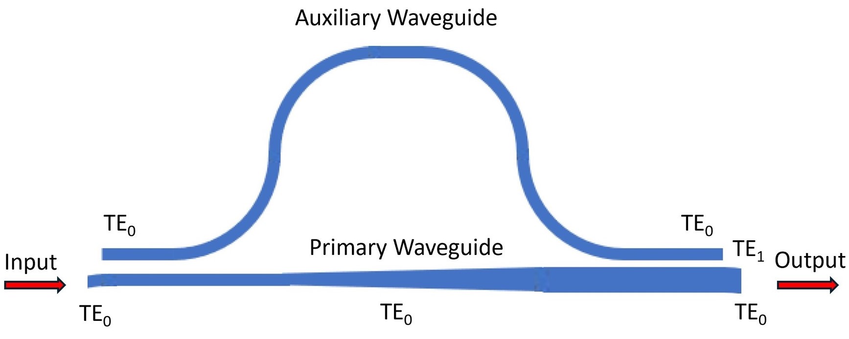
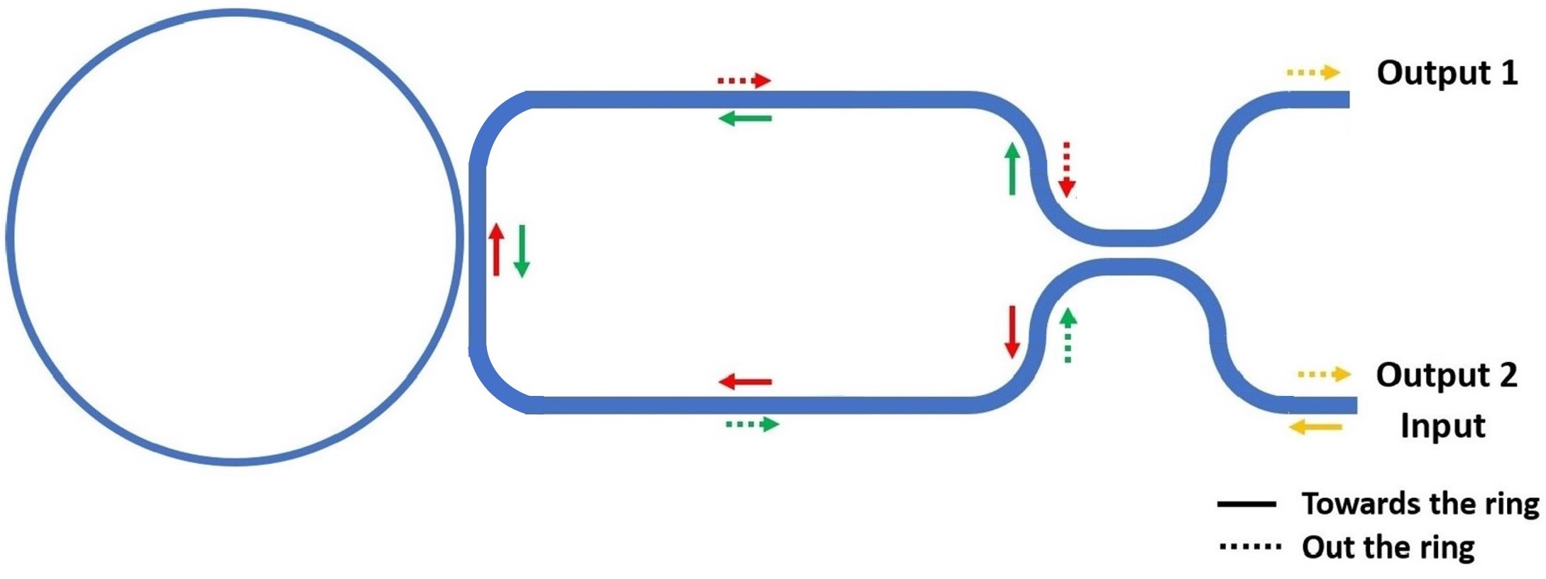
Our system, shown in Fig. 1a, consists of a rotation sensing ring coupled with an IWVA Sagnac interferometer supporting and modes. The interferometer implements a version of inverse weak value amplification using phase front tilters and a multimode 50/50 beam splitter. The setup of this interferometer is discussed in detail in Refs.Steinmetz et al. (2022, 2019); Song et al. (2021). The overall process of the inverse weak value amplification (IWVA) is as follows: the light is injected into the system through the input port on the bottom right of Fig. 1a. Then it goes through a multimode 50/50 beam splitter implemented by waveguide coupling (the point where the two waveguides, on the left of the input and output ports, are very close to each other). Hence, the two beams obtained after the beam splitter go through the left and right arms (lower and upper waveguides respectively in Fig. 1a). As they propagate through these arms, they narrow in transverse profile as the waveguides narrow down in width adiabatically to single mode waveguide. Since the IWVA Sagnac interferometer is coupled with the optical ring, the two beams enter the ring from opposite directions and circulate through the ring independently. Throughout these circulations, the optical ring will carry the wavelengths that match its resonance condition. On the other hand, the radiation coming out of the ring carries change in amplitude and phase and, most importantly, carries information about the rotation of the ring resonator. This is caused by the fact that the optical length of the two opposite paths around the ring are no longer equal due to rotation, as described by the Sagnac effectS. Ezekiel (1977). In this work, we assume that the optical ring has a linear refractive index and, therefore, does not have any nonlinear behavior. The beams coming out of the optical ring then propagate through the spatial phase front tilters discussed in Ref. Song et al. (2021) and shown in Fig. 1b. The spatial phase front tilters operate as follows: the primary and auxiliary waveguides are initially identical single mode waveguides carrying mode. The primary waveguide then couples a small portion of the beam in the mode of the auxiliary waveguide. Then the width of the primary waveguide is increased adiabatically to make it a multimode waveguide that can support both and modes. The light in the mode in the primary waveguide stays in mode since the waveguide is widened adiabatically. Moreover, the widening of the primary waveguide is designed precisely so that its mode supported after the taper is phase matched to the mode in the auxiliary waveguide. Consequently, the light in the auxiliary waveguide couples back into the tapered primary waveguide in mode, giving us a combination of and modes at the end of the primary waveguideSong et al. (2021); Luo et al. (2014); Crespi et al. (2011), as shown in Fig. 1b. After the light beams, containing both and modes, go through the 50/50 beam splitter, we obtain two outputs: one with high intensity light that carries little information about the ring’s rotation (bright port) and the other with lower intensity that carries most of the information about the rotation of the ring (dark port). Finally, at the dark port, light goes through a multimode interfering (MMI) region, the blue box at the top right of Fig. 1a, with two outputs. The optical power difference between the two outputs of the MMI depend on the ratio between the input and modes and contains the desired phase signalSong et al. (2021). We will be discussing these processes in more detail in the following subsections.
(a)
 (b)
(b)
(c)
II.1 Input
To characterize the light entering and propagating through the system, we solve the frequency space Helmholtz equation that gives the mode structure of the traveling electromagnetic fieldsPollock (1995); Griffiths (2021)
| (1) |
where is the time and space dependent electric field, is the wavenumber of the light, and is the frequency-dependent index of refraction. For this setup, we assume the interferometer to be made of rectangular waveguides where the core exists in space for and , and has a refractive index larger than the cladding layer. The electric field propagates in z direction. We assume so that the transverse electric field amplitude is practically independent of the y direction and is expressed as
| (2) |
where is the frequency-dependent wavevector for mode of the electric field with frequency . Assuming the time dependence is suppressed, only the zeroth and first order transverse electric modes ( and ) are required for weak value amplification with integrated photonic devicesSong et al. (2021).
II.2 50/50 Beam Splitter
The input electric field at mode is injected through the left waveguide (the bottom waveguide in the right hand side of the Fig. 1a). Then it goes through a 50/50 beam splitter which is achieved by a directional coupler where the left and right (the top waveguide in the right hand side of the Fig. 1a) waveguides are brought very close to each other so that their electric field modes are coupled and power can transfer periodically between themA. Ghatak (1998). Then the total electric field for the coupled left and right waveguides can be expressed as
| (3) |
where are the electric field modes of the waveguides, are the wave propagation speeds of the left and right waveguides, and and are the normalized amplitudes of the modes in left and right waveguides respectivelyHuang (1994). We assume the modes in the individual waveguides are unperturbed. The generalized coupling constant between any two waveguides and can be expressed asHiremath (2005); A. Ghatak (1998); Haus et al. (1987); Huang (1994)
| (4) |
where and are the transverse electric and magnetic fields in waveguide respectively, is the angular frequency of the field mode, is the vacuum permittivity, with being the refractive index of the two coupled waveguides and being the refractive index of the isolated waveguide . Based on the boundary conditions, and , where Hiremath (2005); A. Ghatak (1998); Haus et al. (1987); Huang (1994). For a 50/50 beam splitter, we then need the length of the directional coupler to be , where is any odd integer. We can take for now. Then, the electric field coming outside the 50/50 beam splitter is in the left arm, and in the right arm for .
We can also express the outgoing electric fields with the transformation matrix that represents the beam splitter interactionsYariv (2000)
| (5) |
where is transmittance, is reflectance and in a lossless system . Moreover, and are the input electric fields incident on the beam splitter from different input ports whereas and are the output electric fields from the beam splitter that are linear combinations of the two input fields.
II.3 Coupling to the Optical Ring
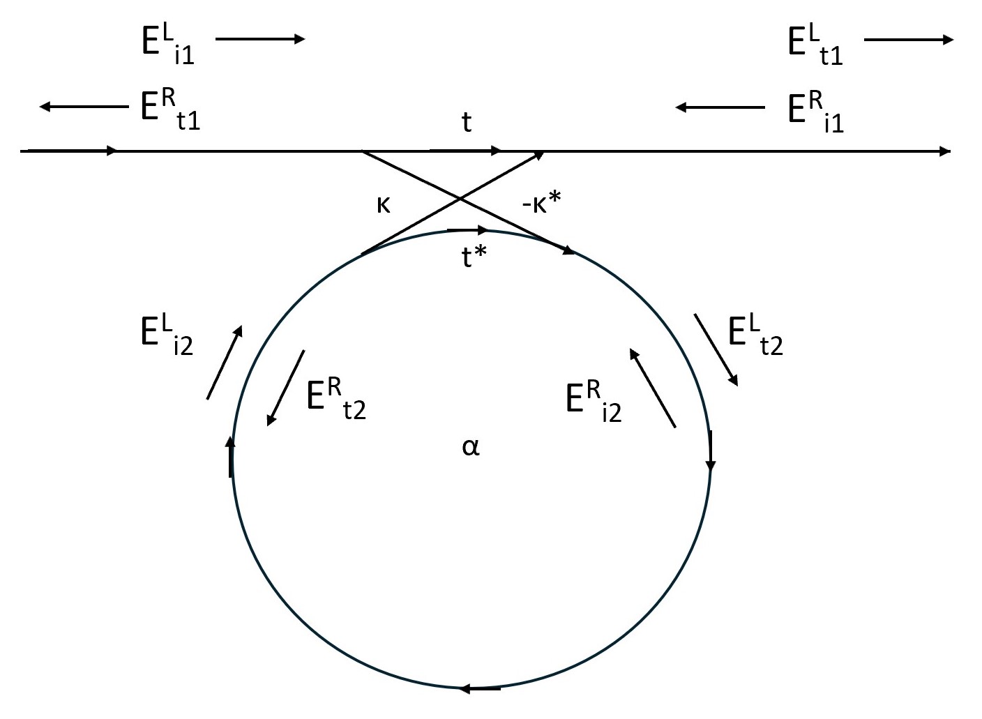
After the two beams propagate through the beam splitter, they travel along the left and right waveguides and narrow in transverse profile as the waveguides gradually decrease in width. Then these beams are incident on the single-mode optical ring from opposite directions through point of contact coupling. Inside the ring, the beams independently circulate through the ring and interfere with themselves. The wavelength in resonance with mode is transferred to the ring, accumulates a Sagnac phase, and exits the ring and propagates through the waveguides to be inverse weak value amplified, which we will discuss in next subsection. The geometry of the coupling with the ring is shown in Fig. 1c. We can approach the coupling of the IWVA Sagnac interferometer and the ring resonator like a beam splitter expressed with the matrix in Eq. (5), where is the transmission amplitude through the coupling region and is the coupling coefficient between the two waveguidesYariv (2000). Assuming a lossless coupling, we can say that . Here, and are the input and output electric fields of the bus waveguide respectively. Similarly, and are the input and output electric fields of the ring resonator respectively. In addition to the beam splitter type relation that describes the geometry of this coupling, we also consider the boundary condition that reveals the relation between the input and output fields of the ring resonator:
| (6) |
where accounts for the loss per cycle around the ring and is expressed as where is the power loss per unit length. gives the geometric phase shift ( is the circumference of the ring, is the radius of the ring and is the wavelength of the light), and gives the phase shift of light traveling in one direction for a single roundtrip due to Sagnac effect where ( is the area of the ring, is the angular rotation rate, and is the speed of light). The Sagnac phase shift has opposite signs for counterpropagating directions. Under the assumption that there are no nonlinear effects present inside the ring, the phase shift due to Sagnac effect is assumed to be linear only. The plus or minus sign on the phase in Eq. (6) depends on whether the direction of the light propagation is with or against the rotation of the ring. Applying this boundary condition to the beam splitter type relation, we can solve for the relation between the input and output electric fields of the linear waveguide for both possible directions of the input field (left or right)
| (7) |
We assume that and are real, and there is no rotation (). We then expand near the resonance condition (), where . Here, is the circumference of the ring for which the resonant wavelengths () satisfy , where is the mode number and an integer. The power coming out of the ring is expressed as
| (8) |
which has an inverse Lorentzian shapeChristopoulos et al. (2019). At resonance (), it is then expressed as
| (9) |
where the input power is lost by a factor of after coming out of the ring resonator. We notice that at the critical coupling limit () and resonance condition (), . Therefore, all the incident light is transferred to the ring and no power is transmitted back to the IWVA Sagnac interferometer.
II.3.1 The Quality Factor
In light of these relations, we can determine the quality factor () which is defined as the ratio between the resonance frequency () and the width (full width at half maximum) of the resonance (). If the frequency of the light is detuned by an amount , from the resonant frequency then the phase shift is where is the circumference of the ring. Then, since the shape of is inverse Lorentzian, we can express the same phase shift from resonance () in terms of , where . Eq. (8) can be rewritten in terms of as
| (10) |
Using the inverse Lorentzian shape of , we obtain its spectral width when the two terms in the denominator of Eq. (10) are equal, giving
| (11) |
Since the resonance frequency is and , we express the loaded quality factor as
| (12) |
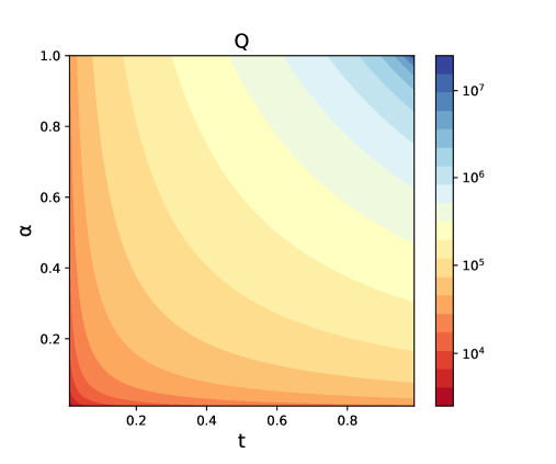
It is important to mention here that diverges when , and deviations from this limit will give a finite value, as shown in Fig. 2. We can see that for a ring radius mm and at nm, we can have a ring resonator with a loaded quality factor up to (, ).
II.3.2 Phase Sensitivity
We would like to explore the phase sensitivity of the field for the values of and near one. We assume that the acquired phase shift is the smallest parameter in the problem to be sensitive to small rotations. We define the deviation parameters , , and such that we will assume them to be small parameters in an expansion. Substituting these parameters, and into Eq. (7), and expanding the equation, we find the resulting electric fields to be
| (13) |
In the limit where we can express this as
| (14) |
where
| (15) |
In the highly overcoupling limit (), we interpret this expression as a phase amplification by a factor of because of the cavity resonance effect. The factor of 2 takes into account the phase shift difference between two opposite directions. The number of roundtrips the light takes around the integrated ring resonator gyroscope is given by Song (2022). In highly overcoupled limit, this corresponds to , which is taken into account by Eq. (15).
When the system is on-resonance () and there is no rotation (), following Eq. (9) and (13), the power coming out of the ring in highly overcoupled limit is
| (16) |
Here we can see that the input power amplitude initially injected into the IWVA Sagnac interferometer is lost by a factor of after coming out of the ring resonator.
The choice of the overcoupling limit as the optimal limit for our system can be justified based on the phase amplification given in Eq. (15). In critical limit (), there is no power coming out of the ring since , and we cannot detect any power, as shown in Eq. (9). In the undercoupling limit (), the phase is amplified by a finite factor . In the overcoupling limit (), the phase amplification is by a factor of , which is finite and much higher than the undercoupling limit. Moreover, all the power is emitted from the optical ring since for a highly overcoupled ring. For these reasons, we operate in the overcoupling limit.
III Results
In order to evaluate the performance of our system (IWVA Sagnac interferometer), we can compare it with the performance of a common Sagnac interferometer coupled to the ring resonator. For this comparison, we will look into the signal-to-noise ratios and phase resolutions of both systems.
III.1 Phase Resolution - Common Sagnac Interferometer
We start our analysis with the common Sagnac interferometer coupled to the ring resonator, as shown in Fig. 3. After the electric field loss and phase shift due to coupling with the ring, we can approximate the electric fields returning to the Sagnac interferometer from the ring resonator from both directions as
| (17) |
| (18) |
based on the relations we have provided in Eq. (16) and (15). Both Sagnac interferometer and IWVA Sagnac interferometer are assumed to be rectangular waveguides described in Section II.1. Therefore, the input electric field is the mode. Thus, . For a Sagnac interferometer with 50/50 beam splitters, the intensity output in both arms are given by . Under the assumption of resonant coupling () and an intentional phase bias of Song (2022), we can express this as
| (19) |
where , , and is the phase amplification. Since we assume that the phase shift is small, we can use small angle approximation and take the difference of the two outputs as our measured signal, the signal per photon detected is expressed as
| (20) |
which yields a linear response in the phase . Consequently, the signal-to-noise ratio (SNR) is given by
| (21) |
where is the number of photons injected into the system and detected, and is the standard deviation (noise) of the two photon detectors measuring and . Since the source of the noise for coherent laser light is the shot-noise, and the two detectors are uncorrelated, the variance is expressed as , where and are the number of photons detected at the two outputs, and . Hence, the standard deviation is . In Sec. III.4, we do an analysis beyond the shot noise limit and discuss other potential sources of error. The use of quantum light, such as squeezed light can further reduce these fluctuations. Then, can be expressed as
| (22) |
At the overcoupling limit where , we can simply assume that is small and finite and . Then we are left with , which is the largest SNR we can get. In overcoupling limit, the loaded quality factor provided in Eq. (12) will be . Therefore, assuming that the ring is lossless, we can express this ideal SNR in overcoupling limit in terms of as
| (23) |
Since a signal producing an SNR of unity indicates the smallest practically resolvable signalBarnett et al. (2003); Dressel et al. (2013), we can find the smallest detectable phase by setting , to find
| (24) |
The minimal angular rotation rate that can be detected can be found from this phase. Via the Sagnac relationS. Ezekiel (1977), we know that the angular rotation rate is , where is the speed of light, and via the geometric phase, we know that . The variables in these relations are defined in Sec. II.3. Hence, the minimal detectable angular rotation rate is given by
| (25) |
From this equation, we see that we can minimize the angular rotation rate by maximizing the product of the radius of the ring () and the loaded quality factor (), for a fixed photon number.
III.2 Phase Resolution - IWVA Sagnac Interferometer
We can now analyze the minimal angular rotation rate for the IWVA Sagnac interferometer discussed in this paper and compare it with the Sagnac interferometer discussed in previous section. The electric fields returning to the IWVA Sagnac interferometer from the ring resonator from both directions are expressed the same as in Eq. (17) and (18), and with the same definition for . As the electric field in each waveguide propagates through the interferometer, it goes through a spatial phase front tilter where a portion of the light in mode is tapped out and then reinjected to the broadened waveguide as modeSong et al. (2021); Steinmetz et al. (2022, 2019), as shown in Fig. 1b and discussed in Sec. II. Hence, the initial electric field mode transforms into
| (26) |
for the left and right waveguide arms. Here, is the amplitude of the mode that was tapped out and coupled to the modeSong et al. (2021); Steinmetz et al. (2022, 2019). Then, modifying the input electric field for Sagnac interferometer, given in Eq. (17) and (18), we can express the electric field in each waveguide of the IWVA Sagnac interferometer as
| (27) |
and
| (28) |
The electric fields in both waveguides will then propagate through the directional coupler we initially used for the input field. We can treat the mode and the mode of the total electric field going into the coupler separately such that the modes of both waveguides will have the coupling constant defined in Sec. II and the modes of both waveguides will have a different coupling constant based on Eq. (4) where and are in mode only. Since is not necessarily the same as , the and modes in both arms will have different coupling constants. Thus, to achieve a 50/50 beam splitter, the coupling length needed for the two modes tends to be different. However, we can benefit from the periodicity of the coupling process and design the length of the directional coupler such that the mode goes through 1/8 (1/4) of a coupling cycle of the electric field (intensity), while the mode goes through 9/8 (5/4) of a coupling cycle of the electric field (intensity)Song et al. (2021). Hence, we obtain a 50/50 beam splitter for both modes simultaneously.
As the beams propagate through the multimode 50/50 beam splitter and interfere before being detected, we obtain two output fields which we call as the “bright” and “dark” modes where
| (29) | |||
| (30) |
Under the assumptions and , we can express the bright mode as
| (31) |
and the dark mode as
| (32) |
It is important to note that in the bright mode, the phase information is carried by the mode, and is suppressed by a factor of . In the dark mode, after renormalization, we have mainly a mode with a small amount of mode added inSteinmetz et al. (2022). Unlike the bright mode, the phase information is carried by the mode in the dark mode, and yields an inverse weak value amplification by a factor of . However, in the high overcoupling limit, the overall input field is reduced by a factor of . Since the phase information is suppressed in bright mode, and amplified in dark mode, we post-select the dark mode for phase measurements. We can then measure the ratio between the modes and by using a multimode interferometer (MMI) at the dark port which has an output power that depends on the mode ratio as discussed in Refs.Steinmetz et al. (2022, 2019), to obtain the measured signal
| (33) |
where is the phase amplification discussed in previous section. While other methods have been discussed in Refs.Steinmetz et al. (2022, 2019), it has been concluded that the mode ratio method is the optimal one and hence, we will use this method in this paper. Similar to the Sagnac interferometer case (Eq. (22)), under the assumption , the SNR of the IWVA Sagnac interferometer can be expressed as
| (34) |
where is the number of photons detected after post-selection, which is less than the number of injected photons. can be expressed in terms of and just like in the Sagnac interferometer case (Eq. (23))
| (35) |
Finally, the minimal angular rotation rate can be derived the same way as in the Sagnac case in Eq. (25)
| (36) |
which can be expressed in terms of the injected photon number
| (37) |
where . We see that when the detected power is the same for the Sagnac interferometer and the IWVA Sagnac interferometer (), the minimal angular rotation rate using the IWVA Sagnac interferometer is more precise by a factor of than using the Sagnac interferometer.
III.3 Comparison - IWVA Sagnac Interferometer vs. Sagnac Interferometer
To see the impact of the inverse weak value amplification achieved with our system, it is important to note that the relation between and is given by
| (38) |
Based on Eq. (32), the power detected for the IWVA Sagnac interferometer is expressed as where is the input power of the IWVA Sagnac interferometer. Since the power and number of photons are directly proportional, the number of detected photons can be expressed as where is the number of photons injected into IWVA Sagnac interferometer. On the other hand, the power detected for the Sagnac interferometer is the same as the power injected into it, . Given that is real, the relation above can be expressed as
| (39) |
Eq. (36), (39), and the direct proportionality between the power and the number of photons show that IWVA Sagnac interferometer has a better SNR and more precise angular rotation rate measurement than a Sagnac interferometer, given that . Then the SNR and the minimum detectable angular rotation rate can both be improved 10 times for . Therefore, we can boost the input power of IWVA Sagnac interferometer to make it perform better than a Sagnac interferometer, at the same detected power value.
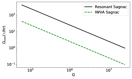
We then compare the simulated angular rotation rate resolutions () as a function of the loaded quality factor in the overcoupling limit where and ranges from 0.05 to 0.99 for IWVA Sagnac interferometer (green dashed line) and Sagnac interferometer (black solid line) in Fig. 4. We take mm, nm, , and the input power to be mW for the Sagnac interferometer, and mW for the IWVA Sagnac interferometer in overcoupling limit . The integration time is taken to be 1s. In both cases we have the same detected power of mW which corresponds to a postselection probability of for the IWVA Sagnac interferometer. The postselection probability can be further reduced in fabrication. This detected power also corresponds to the saturation power of typical detectors. We see that we can gain a factor of 10 or more in precision just from the ability to use a higher power, but keeping the detected power at the saturation point.
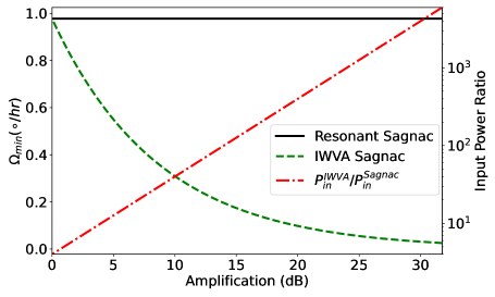
In Fig. 5, we show the angular rotation rate resolution (on the left y-axis) for the Sagnac (solid black line) and the IWVA Sagnac (green dashed line), against the amplification (in dB) of the IWVA Sagnac phase relative to the Sagnac phase (20 ). Compared to Fig. 4, we vary the amplification while keeping the loaded quality factor fixed at ( ). The Sagnac phase is not amplified. Therefore, it is constant, whereas the IWVA Sagnac phase resolution decays below for amplification beyond 20 dB. On the right y-axis, we evaluate the ratio between the input power of the IWVA Sagnac relative to the Sagnac, which is fixed at mW. The input power required for the IWVA Sagnac increases linearly with amplification in log-log scale. This reiterates our previous point: improving the precision of the angular rotation rate comes at the cost of increased power input that has to be injected into the system.
For both Figs. 4 and 5, under expected ideal conditions, for a loaded quality factor ( ) and radius mm, we have a precision of less than hr for IWVA Sagnac interferometer, which exceeds the current state of the artGuo et al. (2012); Dell’Olio et al. (2014); Ciminelli et al. (2010, 2012). Even better precision can be obtained by fabricating a ring resonator with larger radius as we suggest in Eq. (36). Given that an intrinsic of 720 millionLiu et al. (2022) and 422 millionPuckett et al. (2021) has been achieved for a bus-coupled ring resonator in the past, we can obtain even better rotation sensitivity.
III.4 Allan Variance

We finally want to model the uncertainty and error mechanics of the IWVA Sagnac interferometer and compare it to the Sagnac interferometer to see the improvement in error due to IWVA. The errors of these interferometers primarily stem from the noise generated by the measurement instruments, readout detectors. While there are numerous variance techniques available to measure the stochastic errors of inertial sensors, we will be using Allan variance which is one of the simplest and prevalent methods in the fieldEl-Sheimy et al. (2007); Lefevre (2022). For Allan variance calculation, we can assume consecutive data points, each with a time interval . We can divide these samples into clusters, each with consecutive data points (). Each cluster will have a total time interval of . Then, Allan variance () is defined as
| (40) |
where is the index for the cluster number measured in the time interval between and , and is the time averaged angular rotation rate for a given cluster . Based on signal processing theory, Allan variance can also be expressed as the integral of the product of the power spectral density () of the noise in the detector by the square of the Fourier transform of the time gating function over a duration El-Sheimy et al. (2007)
| (41) |
where is the frequency and has the units . In this work we assume that both Sagnac and IWVA Sagnac are white noise limited. This is a reasonable assumption for short measurement time where white noise is the dominant noise source. Hence, the power spectral density will be independent of the frequency 660 (1998), and we can express the Allan deviation () in terms of the angle random walk coefficient ()Gu et al. (2013)
| (42) |
where , but with units . Despite both and have the same dimensions, they have different SI units. Hence, the unit conversion from to is Gu et al. (2013).
As discussed in Refs.Li et al. (2014); Blake and Szafraniec (1997), the noise generated by the optical detectors directly affect the random walk coefficient () of the gryroscope and the noise limit is the detection noiseLefevre (2022). Therefore, stems from the noise of the detectors used for the angular rotation readout. Then, the power spectral density can be expressed as
| (43) |
We know from Sagnac relation, discussed in Sec. II.3, that is the only time dependent variable in detection. Then,
| (44) |
where is the area of the ring resonator. Hence, we can rewrite the power spectral density as
| (45) |
For , and assuming in short time scale for the phase is a delta-correlated random variable, we can express the autocorrelation function as
| (46) |
Since the mean is zero for white noise, . Given that the deviation from average is defined as , we can write the standard deviation as . Then the autocorrelation function can be written as
| (47) |
and the power spectral density becomes
| (48) |
This also shows that Allan deviation is equal to standard deviation when it is white noise limitedLefevre (2022). Finally, is expressed as
| (49) |
It is worth noting that in the overcoupling limit, the detected phase is amplified by and for the Sagnac and IWVA Sagnac respectively. The standard deviation represents the total noise that stems from Johnson, shot and dark current noiseBlake and Szafraniec (1997); Li et al. (2014). Taking these factors into account, and normalizing the Sagnac phase for amplification, in the overcoupling limit, for the Sagnac is given by
| (50) |
and for IWVA Sagnac is
| (51) |
where is the power detected as defined before, is the detector efficiency in units of , is the electron charge, is the Boltzmann constant, is the temperature, is the detector trans-impedance, and is the dark current. Defining an effective area for the ring resonator, where , we can express the Allan deviation (also standard deviation in white noise limit) as
| (52) |
| (53) |
For ( ), , , , , , we find and . We also note that the thermal and shot noise are of the same order at and and much more dominant than the dark current noise at . Other parameters have been specified in previous sections. Improved precision in angular rotation rate readouts as a result of the inverse weak value amplification provides an Allan deviation within an order of magnitude of , and improves the Allan deviation by more than ten times compared to Sagnac interferometer. For a wider range of averaging time , we can see in Fig. 6 that the Allan deviations for both systems have the same negative slope decays in log-log scaleLefevre (2022), but the IWVA Sagnac provides over ten times improvement over the Sagnac at any time.
IV Conclusions
In this work, we have shown that our IWVA Sagnac interferometer allows us to amplify the Sagnac phase shift by a factor of , using only a small fraction of the input power. Compared to a Sagnac interferometer, IWVA Sagnac interferometer has a potential to significantly increase the signal-to-noise ratio and the phase resolution, and reduce the Allan deviation, given that the power detected after post-selection is at the detector saturation point and comparable enough to the power detected at the Sagnac interferometer. This is done through injecting a much larger input power into the IWVA Sagnac interferometer compared to the Sagnac interferometer. We have shown in Fig. 4 that when we inject a larger input power to IWVA Sagnac interferometer and detect the same amount of power as Sagnac interferometer, we can improve the precision of the minimal angular rotation rate by more than a factor of 10. Using Eq. (38), we can also see that under these parameters, we can improve the SNR by more than a factor of 10. Similarly, errors in detection can be reduced by more than ten times. Moreover, for ideal parameters, we obtain a minimum detectable angular rotation rate hr and Allan deviation hr, which enables applications in aerospace and defense industry. Inverse weak value amplification with IWVA Sagnac interferometer developed in this paper can also have potential applications in laser frequency stabilization and other applications in metrology in the future.
Acknowledgements.
This work was supported by NSF award ECCS: 2330328 and Leonardo DRS Technologies.References
- Ezekiel and Arditty (1982) S. Ezekiel and H. J. Arditty, “Fiber-optic rotation sensors. tutorial review,” in Fiber-Optic Rotation Sensors and Related Technologies, edited by Shaoul Ezekiel and Hervé J. Arditty (Springer Berlin Heidelberg, Berlin, Heidelberg, 1982) pp. 2–26.
- Venediktov et al. (2016) V Yu Venediktov, Yu V Filatov, and Egor Vadimovich Shalymov, “Passive ring resonator micro-optical gyroscopes,” Quantum Electronics 46, 437 (2016).
- Chow et al. (1985) WW Chow, J Gea-Banacloche, LM Pedrotti, VE Sanders, Wo Schleich, and MO Scully, “The ring laser gyro,” Reviews of Modern Physics 57, 61 (1985).
- Loukianov (1999) D Loukianov, Optical gyros and their application, Vol. 9 (North Atlantic Treaty Organization Resear Rganization, 1999).
- Post (1967) Evert Jan Post, “Sagnac effect,” Reviews of Modern Physics 39, 475 (1967).
- S. Ezekiel (1977) S. R. Balsamo S. Ezekiel, “Passive ring resonator laser gyroscope,” Applied Physics Letters 30, 478–480 (1977).
- Meyer et al. (1983) R. E. Meyer, S. Ezekiel, D. W. Stowe, and V. J. Tekippe, “Passive fiber-optic ring resonator for rotation sensing,” Optics Letters 8, 644–646 (1983).
- Sagnac (1913) G. Sagnac, “L’ether lumineux demontre par l’effet du vent relatif d’ether dans un interferometre en rotation uniforme.” Comptes Rendus 157, 708–710 (1913).
- Feizpour et al. (2011) Amir Feizpour, Xingxing Xing, and Aephraim M Steinberg, “Amplifying single-photon nonlinearity using weak measurements,” Physical Review Letters 107, 133603 (2011).
- Song et al. (2021) Meiting Song, John Steinmetz, Yi Zhang, Juniyali Nauriyal, Kevin Lyons, Andrew N Jordan, and Jaime Cardenas, “Enhanced on-chip phase measurement by inverse weak value amplification,” Nature Communications 12, 6247 (2021).
- Steinmetz et al. (2022) John Steinmetz, Kevin Lyons, Meiting Song, Jaime Cardenas, and Andrew N Jordan, “Enhanced on-chip frequency measurement using weak value amplification,” Optics Express 30, 3700–3718 (2022).
- Lyons et al. (2018) Kevin Lyons, John C Howell, and Andrew N Jordan, “Noise suppression in inverse weak value-based phase detection,” Quantum Studies: Mathematics and Foundations 5, 579–588 (2018).
- Steinmetz et al. (2019) John Steinmetz, Kevin Lyons, Meiting Song, Jaime Cardenas, and Andrew N Jordan, “Precision frequency measurement on a chip using weak value amplification,” in Quantum Communications and Quantum Imaging XVII, Vol. 11134 (SPIE, 2019) pp. 102–111.
- Aharonov et al. (1988) Yakir Aharonov, David Z Albert, and Lev Vaidman, “How the result of a measurement of a component of the spin of a spin-1/2 particle can turn out to be 100,” Physical Review Letters 60, 1351 (1988).
- Jordan et al. (2014) Andrew N Jordan, Julián Martínez-Rincón, and John C Howell, “Technical advantages for weak-value amplification: when less is more,” Physical Review X 4, 011031 (2014).
- Dixon et al. (2009) P Ben Dixon, David J Starling, Andrew N Jordan, and John C Howell, “Ultrasensitive beam deflection measurement via interferometric weak value amplification,” Physical Review Letters 102, 173601 (2009).
- Dell’Olio et al. (2014) Francesco Dell’Olio, Teresa Tatoli, Caterina Ciminelli, and Mario N Armenise, “Recent advances in miniaturized optical gyroscopes,” Journal of the European Optical Society-Rapid Publications 9, 14013i (2014).
- Hosten and Kwiat (2008) Onur Hosten and Paul Kwiat, “Observation of the spin hall effect of light via weak measurements,” Science 319, 787–790 (2008).
- Starling et al. (2010) David J Starling, P Ben Dixon, Andrew N Jordan, and John C Howell, “Precision frequency measurements with interferometric weak values,” Physical Review A—Atomic, Molecular, and Optical Physics 82, 063822 (2010).
- Luo et al. (2014) Lian-Wee Luo, Noam Ophir, Christine P Chen, Lucas H Gabrielli, Carl B Poitras, Keren Bergmen, and Michal Lipson, “Wdm-compatible mode-division multiplexing on a silicon chip,” Nature Communications 5, 1–7 (2014).
- Crespi et al. (2011) Andrea Crespi, Roberta Ramponi, Roberto Osellame, Linda Sansoni, Irene Bongioanni, Fabio Sciarrino, Giuseppe Vallone, and Paolo Mataloni, “Integrated photonic quantum gates for polarization qubits,” Nature Communications 2, 566 (2011).
- Song (2022) Meiting Song, Integrated Photonic Devices with Inverse Weak Value Amplification for Precision Metrology, Ph.D. thesis (2022).
- Yariv (2000) Amnon Yariv, “Universal relations for coupling of optical power between microresonators and dielectric waveguides,” Electronics Letters 36, 321–322 (2000).
- Pollock (1995) C. R. Pollock, Fundamentals of Optoelectronics (Irwin, 1995).
- Griffiths (2021) David J Griffiths, “Introduction to electrodynamics fourth edition,” (2021).
- A. Ghatak (1998) K. Thyagarajan A. Ghatak, “An introduction to fiber optics,” Cambridge University (1998).
- Huang (1994) Wei-Ping Huang, “Coupled-mode theory for optical waveguides: an overview,” Journal of the Optical Society of America A 11, 963–983 (1994).
- Hiremath (2005) Kirankumar Rajshekhar Hiremath, Coupled mode theory based modeling and analysis of circular optical microresonators (Kirankumar R. Hiremath, 2005).
- Haus et al. (1987) H Haus, W Huang, S Kawakami, and N Whitaker, “Coupled-mode theory of optical waveguides,” Journal of Lightwave Technology 5, 16–23 (1987).
- Christopoulos et al. (2019) Thomas Christopoulos, Odysseas Tsilipakos, Georgios Sinatkas, and Emmanouil E Kriezis, “On the calculation of the quality factor in contemporary photonic resonant structures,” Optics Express 27, 14505–14522 (2019).
- Barnett et al. (2003) Stephen M Barnett, Claude Fabre, and Agnes Maıtre, “Ultimate quantum limits for resolution of beam displacements,” The European Physical Journal D-Atomic, Molecular, Optical and Plasma Physics 22, 513–519 (2003).
- Dressel et al. (2013) Justin Dressel, Kevin Lyons, Andrew N Jordan, Trent M Graham, and Paul G Kwiat, “Strengthening weak-value amplification with recycled photons,” Physical Review A—Atomic, Molecular, and Optical Physics 88, 023821 (2013).
- Guo et al. (2012) Lijun Guo, Bangren Shi, Chen Chen, and Meng Zhao, “A large-size sio2 waveguide resonator used in integration optical gyroscope,” Optik 123, 302–305 (2012).
- Ciminelli et al. (2010) Caterina Ciminelli, Francesco Dell’Olio, Carlo E Campanella, and Mario N Armenise, “Photonic technologies for angular velocity sensing,” Advances in Optics and Photonics 2, 370–404 (2010).
- Ciminelli et al. (2012) Caterina Ciminelli, Francesco Dell’Olio, and Mario N Armenise, “High-q spiral resonator for optical gyroscope applications: numerical and experimental investigation,” IEEE Photonics Journal 4, 1844–1854 (2012).
- Liu et al. (2022) Kaikai Liu, Naijun Jin, Haotian Cheng, Nitesh Chauhan, Matthew W Puckett, Karl D Nelson, Ryan O Behunin, Peter T Rakich, and Daniel J Blumenthal, “Ultralow 0.034 dB/m loss wafer-scale integrated photonics realizing 720 million Q and 380 W threshold brillouin lasing,” Optics Letters 47, 1855–1858 (2022).
- Puckett et al. (2021) Matthew W Puckett, Kaikai Liu, Nitesh Chauhan, Qiancheng Zhao, Naijun Jin, Haotian Cheng, Jianfeng Wu, Ryan O Behunin, Peter T Rakich, Karl D Nelson, et al., “422 million intrinsic quality factor planar integrated all-waveguide resonator with sub-mhz linewidth,” Nature Communications 12, 934 (2021).
- El-Sheimy et al. (2007) Naser El-Sheimy, Haiying Hou, and Xiaoji Niu, “Analysis and modeling of inertial sensors using allan variance,” IEEE Transactions on Instrumentation and Measurement 57, 140–149 (2007).
- Lefevre (2022) Herve C Lefevre, The fiber-optic gyroscope (Artech House, 2022).
- 660 (1998) “Ieee standard specification format guide and test procedure for single-axis interferometric fiber optic gyros,” IEEE Std 952-1997 , 1–84 (1998).
- Gu et al. (2013) Hong Gu, Shuhong Li, Fuzhong Wang, and Haiming Zhang, “Random noise study of the digital closed-loop fiber optic gyroscope,” in International Symposium on Photoelectronic Detection and Imaging 2013: Fiber Optic Sensors and Optical Coherence Tomography, Vol. 8914 (SPIE, 2013) p. 891402.
- Li et al. (2014) Yongxiao Li, Zinan Wang, Yi Yang, Chao Peng, Zhenrong Zhang, and Zhengbin Li, “A multi-frequency signal processing method for fiber-optic gyroscopes with square wave modulation,” Optics Express 22, 1608–1618 (2014).
- Blake and Szafraniec (1997) J Blake and B Szafraniec, “Random noise in pm and depolarized fiber gyros,” in Optical Fiber Sensors (Optica Publishing Group, 1997) p. OWB2.