BiLO: Bilevel Local Operator Learning for PDE Inverse Problems. Part II: Efficient Uncertainty Quantification with Low-Rank Adaptation

Abstract

Uncertainty quantification and inverse problems governed by partial differential equations (PDEs) are central to a wide range of scientific and engineering applications. In this second part of a two part series, we extend Bilevel Local Operator Learning (BiLO) for PDE-constrained optimization problems developed in Part 1 to the Bayesian inference framework. At the lower level, we train a network to approximate the local solution operator by minimizing the local operator loss with respect to the weights of the neural network. At the upper level, we sample the PDE parameters from the posterior distribution. We achieve efficient sampling through gradient-based Markov Chain Monte Carlo (MCMC) methods and low-rank adaptation (LoRA). Compared with existing methods based on Bayesian neural networks, our approach bypasses the challenge of sampling in the high-dimensional space of neural network weights and does not require specifying a prior distribution on the neural network solution. Instead, uncertainty propagates naturally from the data through the PDE constraints. By enforcing strong PDE constraints, the proposed method improves the accuracy of both parameter inference and uncertainty quantification. We analyze the dynamic error of the gradient in the MCMC sampler and the static error in the posterior distribution due to inexact minimization of the lower level problem and demonstrate a direct link between the tolerance for solving the lower level problem and the accuracy of the resulting uncertainty quantification. Through numerical experiments across a variety of PDE models, we demonstrate that our method delivers accurate inference and quantification of uncertainties while maintaining high computational efficiency.

1 Introduction

Quantifying uncertainty in physical systems is crucial for informed decision-making across various disciplines. Key applications include seismic imaging [1, 2, 3, 4], personalized medicine [5, 6], climate modeling [7], and engineering design [8]. These fields frequently require solving PDE inverse problems within a Bayesian framework [9], where the objective is to estimate the posterior distribution of model parameters given observed data. Typically, this process involves sampling PDE parameters and repeatedly solving the forward PDE. A related approach, PDE-constrained optimization, aims to identify a single optimal parameter estimate, thus offering computational efficiency but lacking the ability to quantify uncertainty.

This is the second paper in a two-part series. In Part I, we develop a constrained optimization framework to solve inverse PDE problems using deep learning methods [10]. Here in Part II, we extend this approach to Bayesian inference frameworks building upon the core methodology developed in Part I, while leveraging transfer learning techniques to enhance sampling efficiency.

Addressing Bayesian PDE inverse problems involves two design choices: the PDE solver and the sampling method. PDE solutions can be computed using numerical methods (such as finite difference or finite element methods), physics-informed neural networks (PINNs)[11], or neural operators such as Fourier Neural Operator [12] and DeepONet [13]. Each approach has its advantages and limitations. Numerical methods provide fast, accurate, and convergent solutions but can struggle with high-dimensional PDEs [14]. PINNs offer a mesh-free approach, effective in some higher-dimensional PDE problems, and a unified framework for inverse problems. Neural operators, while requiring many synthetic numerical solutions to train, enable rapid evaluations and serve as PDE surrogates; however, their accuracy remains relatively low, especially outside the distribution of the training dataset. For sampling, Markov Chain Monte Carlo (MCMC) [15] methods can be either gradient-based (e.g., Hamiltonian Monte Carlo [16, 17, 18]) or derivative-free (e.g., Ensemble Kalman Sampling [19]). Gradient-based methods efficiently explore posterior distributions, but computing the gradient can be expensive (compared with gradient-free approaches) or impractical (e.g., when the PDE solver is a black box).

Numerical PDE solvers can be paired with gradient-based sampling methods. The Adjoint Method computes gradients of the likelihood function with respect to PDE parameters [20]. While the adjoint method ensures accurate solutions and gradients, deriving adjoint equations for complex PDEs can be challenging and solving both the forward and adjoint equations numerically can be computationally intensive. When only the forward solver is available, it is more practical to use derivative-free sampling methods such as Ensemble Kalman Sampling (EnKS), which employ ensembles of interacting particles to approximate posterior distributions [19]. Additionally, variants of Ensemble Kalman Inversion (EnKI) can efficiently estimate the first two moments in Bayesian settings [21, 22, 23].

Among neural PDE solvers, Physics-Informed Neural Networks (PINNs) [11] have become widely adopted. In PINNs, the PDE residual is enforced as a soft constraint. By minimizing a weighted sum of the data loss and the PDE residual loss, PINNs can fit the data, solve the PDE, and infer the parameters at the same time. For uncertainty quantification, Bayesian PINNs (BPINNs) [24] represent PDE solutions using Bayesian neural networks, and use Hamiltonian Monte Carlo (HMC) to sample the joint posterior distributions of PDE parameters and neural network weights. Derivative-free methods, such as EnKI, can also be effectively combined with neural PDE solvers, as demonstrated in PDE-constrained optimization problems [25] and Bayesian PINNs [23].

Neural Operators (NOs) approximate the PDE solution operator (parameter-to-solution map), providing efficient surrogate models for forward PDE solvers [26]. Once trained, these surrogates integrate seamlessly with Bayesian inference frameworks, leveraging rapid neural network evaluations for posterior distribution sampling using both gradient-based and derivative-free methods [27, 28, 29]. Prominent examples include the Fourier Neural Operator (FNO) [12, 30, 31, 32], Deep Operator Network (DeepONet) [13, 33], and In-Context Operator (ICON) [34], among others [35, 36]. Nevertheless, neural operator performance heavily depends on the training dataset, potentially limiting accuracy in PDE solutions and consequently degrading posterior distribution fidelity [37].

In this work, we focus explicitly on addressing PDE inverse problems using the Bayesian framework through neural PDE solvers and gradient-based MCMC methods. The key contributions of this work are as follows:

Main Contributions

• We introduce a Bilevel local operator (BiLO) learning approach that enforces strong PDE constraints, leading to improved accuracy in uncertainty quantification and parameter inference.

• We avoid direct sampling in the high-dimensional space of Bayesian neural networks, leading to more efficient sampling of unknown PDE parameters or functions.

• We apply Low-Rank Adaptation (LoRA)[38] to enhance both efficiency and speed in fine-tuning and sampling, significantly reducing computational cost while maintaining accuracy.

• We prove there is a direct link between the tolerance for solving the lower level problem to approximate the local solution operator and the accuracy of the resulting uncertainty quantification. In particular, we estimate the error in the posterior distribution due to inexact minimization of the lower level problem.

The outline of the paper is as follows. In Sec. 2, we present the BiLO framework for Bayesian inference with low rank adaption (LoRA). We highlight the differences between our approach and those used in BPINNs. In Sec. 3, we present numerical results for a variety of PDE inverse problems, and compare the results with BPINNs. In Sec. 4, we summarize the results. In the Appendices, we present theoretical analyses and additional numerical results.

2 Method

In this section, we present the BiLO framework for Bayesian inference with low-rank adaptation (LoRA). The section is organized as follows. In 2.1 we formulate the PDE-based Bayesian inverse problem as a bi-level optimization problem, where the upper level involves sampling the PDE parameters, and the lower level trains a neural network to approximate the local operator. In 2.2, we describe the neural network architecture used to approximate the local operator. In 2.3, we provide a brief overview of the Hamiltonian Monte Carlo (HMC) algorithm in a general context, independent of the BiLO framework. In 2.4, we present our main algorithm—BiLevel Local Operator Hamiltonian Monte Carlo (BiLO-HMC)—along with several theoretical results. In 2.5, we describe the pre-training and fine-tuning workflow, and introduce the low-rank adaptation (LoRA) technique used to accelerate inference. In 2.6, we highlight the differences between our approach and Bayesian physics-informed neural networks (BPINNs) [24].

2.1 Bi-Level Local Operator for Bayesian Inference

Let $u:\Omega\to\mathbb{R}$ be a function defined over a domain $\Omega\subset\mathbb{R}^{d}$ satisfying some boundary conditions. Suppose $u$ is governed by some constraints that include the PDE, boundary conditions, and initial conditions,

$$\mathcal{F}(D^{k}u(\mathbf{x}),...,Du(\mathbf{x}),u(\mathbf{x}),\theta)=\mathbf{0},$$ (1)

where $D^{k}$ is the $k$-th order derivative operator and $\theta$ are the PDE parameters. We assume that the solution is unique for each $\theta$ and that the solution depends smoothly on $\theta$. The precise assumptions on the function space will be specified when a theorem is presented.

We consider functions of the form $u(\mathbf{x},\theta)$ and define the residual function

$$r(\mathbf{x},\theta):=\mathcal{F}(D^{k}u(\mathbf{x},\theta),...,Du(\mathbf{x},\theta),u(\mathbf{x},\theta),\theta)\\$$ (2)

The dependence of $r$ on $u$ is not explicitly indicated for brevity. A function $u(\mathbf{x},\theta)$ is called a full operator (hereafter referred to as the “operator”) if $r(\mathbf{x},\theta)=0$ for all $\theta$; that is, it solves the PDE for all $\theta$ in some admissible set. We define $u$ as a local operator at $\theta$ if the following two conditions hold:

• Condition 1: $r(\mathbf{x},\theta)=\mathbf{0}$.

• Condition 2: $\gradient_{\theta}r(\mathbf{x},\theta)=d_{\theta}\mathcal{F}(D^{k}u(\mathbf{x},\theta),...,Du(\mathbf{x},\theta),u(\mathbf{x},\theta),\theta)=\mathbf{0}$.

where $d_{\theta}$ is the total derivative with respect to $\theta$.

For Bayesian inference, let $P(\theta)$ be the prior distribution of the PDE parameters, let $D$ be the observed data, $P(D|\theta)$ be the likelihood of the observed data given the PDE parameters, and $P(\theta|D)$ be the posterior distribution of the PDE parameters. For example, if we assume that the data is observed at $N$ collocation points $\mathbf{x}_{i}\in\Omega$, and the observation is corrupted by Gaussian noise with mean 0 and variance $\sigma_{d}^{2}$, then the likelihood of the observed data $D$ given the PDE parameters $\theta$ is

$$P(D|\theta)=\prod_{i=1}^{N}\frac{1}{\sqrt{2\pi\sigma_{d}^{2}}}\exp\left(-\frac{1}{2\sigma_{d}^{2}}\left|u(\mathbf{x}_{i},\theta)-\hat{u}(\mathbf{x}_{i})\right|^{2}\right)$$ (3)

By Bayes’ theorem, $P(\theta|D)\propto P(D|\theta)P(\theta)$. The potential energy, $U(\theta)$, is defined as the negative of the log-posterior distribution

$$U(\theta)=-\log P(\theta|D)=-\log P(D|\theta)-\log P(\theta)$$ (4)

The potential energy $U$ is a functional of the PDE solution $u(\cdot,\theta)$, and thus ultimately depends only on the PDE parameters $\theta$. Sampling the posterior distribution with gradient-based MCMCs, such as Langevin Dynamics (LD) or Hamiltonian Monte Carlo (HMC), requires computing the gradient of the potential energy $\nabla_{\theta}U(\theta)$ to effectively explore the posterior distribution.

In this work, we represent the local operator by a neural network $u(\mathbf{x},\theta;W)$, where $W$ are the weights of the neural network. Then $u(\cdot,\theta;W)$ is the approximate solution of the PDE at $\theta$. The detailed architecture of the neural network will be described in Section 2.2. The residual function depends on the weights of the neural network $W$, and can be written as $r(\mathbf{x},\theta;W)$. The two conditions for $u$ to be a local operator at $\theta$ lead to the definition of the local operator loss $\mathcal{L}_{\text{LO}}$:

$$\mathcal{L}_{\text{LO}}(\theta,W)=\norm{r(\cdot,\theta;W)}^{2}_{2}+w_{\rm rgrad}\norm{\nabla_{\theta}r(\cdot,\theta;W)}^{2}_{2},$$ (5)

The 2-norm of the residual and its gradient with respect to $\theta$ are approximated by the Mean Squared Error (MSE) of the residual and the residual-gradient loss at a set of collocation points. The weight $w_{\rm rgrad}>0$ is a scalar hyperparameter that controls the relative importance of the residual gradient loss. In theory, both terms can be sufficiently minimized to near zero. For fixed $\theta$, by minimizing the local operator loss $\mathcal{L}_{\text{LO}}(\theta,W)$ with respect to the weights $W$, we approximate the local operator $u(\mathbf{x},\theta;W)$ around $\theta$. Since $U$ depends on the approximate solution of the PDE $u(\cdot,\theta;W)$ at $\theta$, we can also write the potential energy as $U(\theta,W)$.

We consider the following Bayesian inference problem:

$$\begin{cases}\theta\sim\exp(-U(\theta,W^{*}(\theta)))\\ W^{*}(\theta)=\arg\min_{W}\mathcal{L}_{\text{LO}}(\theta,W)\\ \end{cases}$$ (6)

At the lower level, we train a network to approximate the local operator $u(\mathbf{x},\theta;W)$ by minimizing the local operator loss with respect to the weights of the neural network. At the upper level, we sample the PDE parameters $\theta$ from the posterior distribution $P(\theta|D)$.

Hereafter, for notational convenience, we assume that quantities that do not depend explicitly on $W$ are exact. For example, $u(\mathbf{x},\theta)$ is used to denote the exact local or global operator (depending on context), and $u(\cdot,\theta)$ is the exact solution of the PDE at $\theta$. PDE solutions computed using numerical methods (e.g., finite element or finite difference methods) on a fine grid are also considered exact, as they are generally more accurate than neural network approximations [14, 39]. $U(\theta)$ denotes the potential energy of the exact PDE solution $u(\cdot,\theta)$ given $\theta$. The explicit presence of $W$ is taken to indicate neural network approximations of the corresponding quantities. For example, $u(\mathbf{x},\theta;W)$ is the neural network approximation of the local operator at $\theta$, and $U(\theta,W)$ denotes the potential energy of the function $u(\cdot,\theta;W)$.

A schematic of the BiLO framework is shown in Figure 1. The figure is based on a model boundary value problem $-\theta u_{xx}=\sin(\pi x)$ with the Dirichlet boundary condition $u(0)=u(1)=0$. In this case, the full operator is given by $u(x,\theta)=\sin(\pi x)/(\pi^{2}\theta)$, which solves the PDE for all $\theta>0$.

Figure 1 panel (A) illustrates the upper-level problem: the goal is to sample the PDE parameters $\theta$ from the posterior distribution. For gradient-based MCMC methods, we need to compute the gradient of the potential energy $\nabla_{\theta}U(\theta)$ at various values of $\theta$ (orange arrows). Therefore, at any fixed $\theta$, we need access to the local behavior of the potential energy, shown as the blue strip near $\theta_{1}$ and $\theta_{2}$.

In Figure 1 panel (B), the gray surface is the full PDE operator $u(x,\theta)$. At some particular $\theta_{1}$, the local operator $u(x,\theta_{1})$ approximates a small neighborhood of the full operator near $\theta_{1}$ (blue surface). The condition of the local operator is that the residual and the gradient of the residual with respect to $\theta$ are both zero at any fixed $\theta$. Knowing the local operator at $\theta_{1}$ allows us to compute the gradient of the potential energy at $\theta_{1}$.

Figure 1 panel (C) illustrates the lower-level problem: we train a neural network to approximate the local operator at different $\theta$, e.g. $\theta_{1}$ and $\theta_{2}$. The local operator at $\theta_{1}$ is approximated by a neural network $u(x,\theta_{1};W)$ and is obtained by minimizing the local operator loss $\mathcal{L}_{\text{LO}}(\theta_{1},W)$.

Since we require local operators at different $\theta$ during sampling (e.g., $\theta_{1}$ and $\theta_{2}$), the neural network must be retrained for each $\theta$ to obtain corresponding weights $W(\theta_{1})$ and $W(\theta_{2})$ The weight matrices in the hidden layers of the neural network have dimension $p\times p$, where $p$ is the number of hidden neurons and is usually a large number. Updating the full set of weights $W$ at each sampling step can be computationally expensive, especially when many sampling steps are required. We can reduce the computational cost by using the low-rank adaptation (LoRA) technique [38], which assumes that the change between the weights is low-rank; that is, $W^{*}(\theta_{2})=W^{*}(\theta_{1})+AB$, where $A\in\mathbb{R}^{p\times r}$ and $B\in\mathbb{R}^{r\times p}$ and $r$ is much smaller than $p$. LoRA drastically reduces the number of trainable parameters in the neural network without significantly affecting the performance of the neural network. Further details on the network architecture and the LoRA method are provided in Sections 2.2 and 2.5

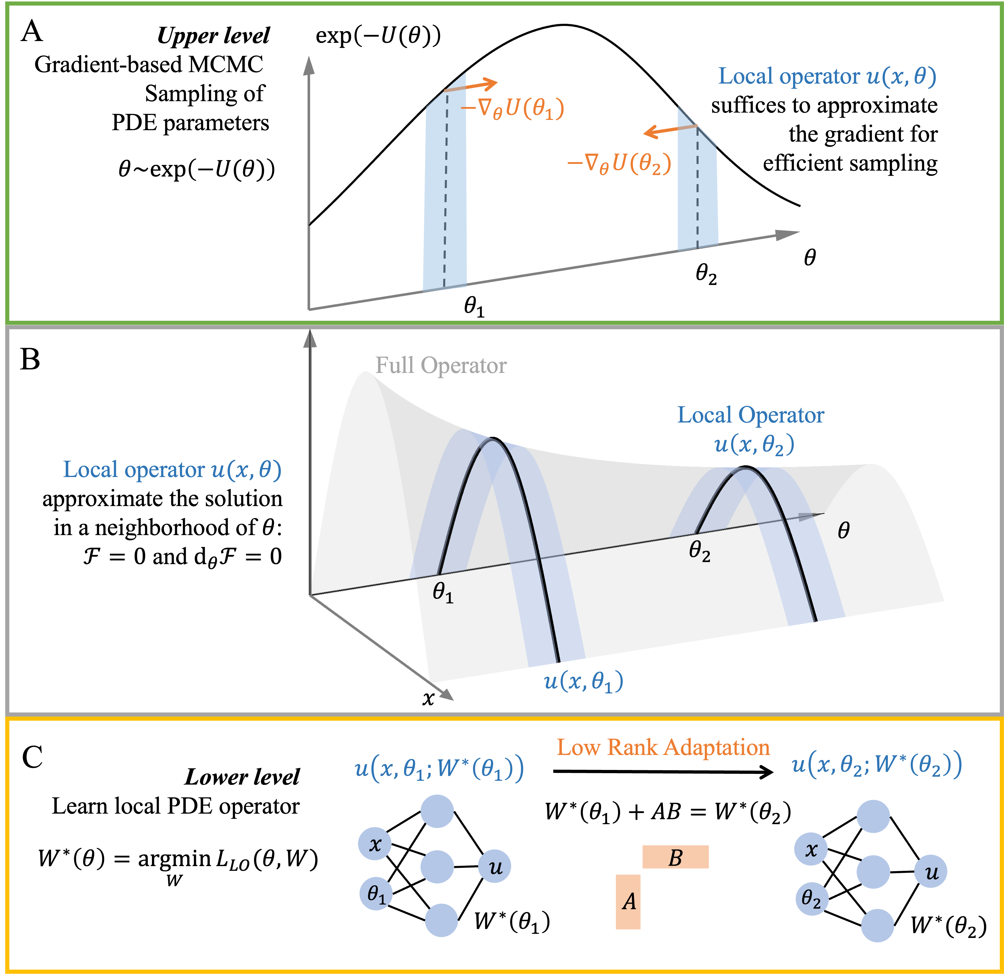
Figure 1: A schematic for solving the Bayesian PDE inverse problem using BiLO and LoRA. (A) At the upper level, we sample the PDE parameters $\theta$ from the posterior distribution using gradient-based MCMC. (B) The full operator $u(x,\theta)$ (gray surface) and its local approximation $u(x,\theta_{1})$ and $u(x,\theta_{2})$ (blue surface), which satisfies vanishing residual and residual gradient conditions. The local operators suffices to compute the gradient of the potential energy $U(\theta)$ at $\theta_{1}$ and $\theta_{2}$. (C) At the lower level, we train the neural network to approximate the local operator (blue surface) at different $\theta$. As $\theta$ changes, only low rank adaptation (LoRA) is used to update the neural network weights $W$.

2.2 Architecture

The representation of the local operator $u(\mathbf{x},\theta;W)$ is based on a multi-layer perceptron (MLP) neural network. We define an embedding layer that maps the inputs $\mathbf{x}\in\Omega\subset\mathbb{R}^{d}$ and the PDE parameters $\theta\in\mathbb{R}^{m}$ to a high-dimensional vector $\mathbf{y}\in\mathbb{R}^{p}$, using an affine transformation followed by an element-wise nonlinear activation function (e.g., tanh) $\sigma$:

$$\mathbf{y}=\sigma(\mathbf{W}^{(0)}\mathbf{x}+\mathbf{R}\theta+\mathbf{b}^{(0)}),$$ (7)

where $\mathbf{W}^{(0)}\in\mathbb{R}^{p\times d}$ is the embedding matrix applied to $\mathbf{x}$, $\mathbf{R}\in\mathbb{R}^{p\times m}$ is the embedding matrix applied to $\theta$, and $\mathbf{b}^{(0)}\in\mathbb{R}^{p}$ is the bias vector.

We use an MLP that takes $\mathbf{y}$ as input, and define $m(\mathbf{x},\theta;W)$ as its raw output:

$$\mathbf{h}^{(0)} =\mathbf{y},$$

$$\mathbf{h}^{(l)} =\sigma\left(\mathbf{W}^{(l)}\mathbf{h}^{(l-1)}+\mathbf{b}^{(l)}\right),\quad\text{for }l=1,\dots,L,$$

$$m(\mathbf{x},\theta;W) =\mathbf{W}^{(L+1)}\mathbf{h}^{(L)}+\mathbf{b}^{(L+1)},$$

where $\mathbf{W}^{(l)}\in\mathbb{R}^{d_{l}\times d_{l-1}}$, $\mathbf{b}^{(l)}\in\mathbb{R}^{d_{l}}$ are the weights and biases for layer $l$. The output dimension is $d_{L+1}=1$. For simplicity, we assume all hidden layers have the same dimension as the embedding dimension $p$, i.e., $d_{l}=p$ for $l=1,\dots,L$. $W=\{\mathbf{W}^{(l)},\mathbf{b}^{(l)}\}_{l=0}^{L+1}$ denotes the full set of trainable parameters.

A final transformation can be applied to the output of the MLP to enforce the boundary condition or the initial condition [40, 41]. For example, if the PDE is defined on a unit interval $[0,1]$ with Dirichlet boundary conditions $u(0)=u(1)=0$, the BiLO solution can be represented as

$$u(\mathbf{x},\theta;W)=m(\mathbf{x},\theta;W)(1-\mathbf{x})\mathbf{x},$$ (8)

Alternatively, the boundary condition can be enforced by an additional loss term.

A key design choice in BiLO is that the embedding matrix $\mathbf{R}$ should be non-trainable to prevent it from collapsing to zero. Otherwise, $\mathcal{L}_{\rm rgrad}(W,\theta)$ can be made zero simply by setting $\mathbf{R}$ to be 0. $\mathbf{R}$ can be randomly initialized in the same way as the other weights [42]. We describe the architecture in detail in this section—although standard except for the embedding layer—to facilitate the explanation of Low-Rank Adaptation in Section 2.5.

2.3 Review of Markov Chain Monte Carlo (MCMC) Methods

In this section, we provide a quick overview of the sampling methods that appeared in this work, including the Metropolis-Hastings (MH) algorithm and the Hamiltonian Monte Carlo (HMC). These methods are Markov Chain Monte Carlo (MCMC) methods that generate samples from a target distribution by constructing a Markov chain whose stationary distribution is the target distribution.

We present these methods independent of the BiLO framework. This is assuming that we have the parameter-to-solution map $\theta\mapsto u(\cdot,\theta)$, and we can compute the potential energy $U(\theta)$ and the gradient $\nabla_{\theta}U(\theta)$ accurately. With this assumption, in this section, we temporarily drop the dependence of the potential energy $U$ on the neural network weights $W$. We will reintroduce the dependence on $W$ in Section 2.4 when we describe how to incorporate these sampling methods in the BiLO framework.

Metropolis-Hastings (MH) Algorithm

The Metropolis-Hastings (MH) algorithm [15] is a classical and simple MCMC method. It requires a proposal distribution $Q(\theta^{\prime}|\theta)$ to propose new samples $\theta^{\prime}$ given the current sample $\theta$. The proposal is then accepted or rejected based on the changes in the potential energy. Algorithm 1, given below, summarizes the MH algorithm for sampling from the potential energy $U(\theta)$. For simple proposal distributions, such as Gaussian or uniform distributions, MH is easy to implement and does not require computing the gradient of the potential energy. However, it can be inefficient as the acceptance rate may be low [16]. In this work, the MH algorithm is coupled with an accurate numerical PDE solver, and serves primarily as a reference method to assess the accuracy of alternative sampling approaches.

Algorithm 1 Metropolis-Hastings (MH) Algorithm

1:Initial state $\theta^{(0)}$, proposal distribution $Q(\theta^{\prime}|\theta)$, number of iterations $N$

2:for $k=1,2,\dots,N$ do

3:  Sample $\theta^{\prime}\sim Q(\cdot|\theta^{(k-1)})$

4:  Compute acceptance probability

$$\alpha=\min\left(1,\exp\left[U(\theta^{(k-1)})-U(\theta^{\prime})\right]\cdot\frac{Q(\theta^{(k-1)}|\theta^{\prime})}{Q(\theta^{\prime}|\theta^{(k-1)})}\right)$$

5:  Sample $u\sim U[0,1]$

6:  if $u<\alpha$ then

7:   Accept the proposal: $\theta^{(k)}\leftarrow\theta^{\prime}$

8:  else

9:   Reject the proposal: $\theta^{(k)}\leftarrow\theta^{(k-1)}$

10:  end if

11:end for

Hamiltonian Monte Carlo (HMC)

In HMC, an auxiliary momentum variable $\rho$ is introduced, and the Hamiltonian is defined as

$$H(\theta,\rho)=U(\theta)+K(\rho)=-\log P(\theta|D)+\frac{1}{2}\rho^{T}M^{-1}\rho,$$ (9)

where $M$ is the mass matrix, which is symmetric and positive definite. $M$ can be user-defined or adaptively learned in a warmup phase. HMC samples from the joint distribution $P(\theta,\rho)\propto\exp(-H(\theta,\rho))$ from the Hamiltonian dynamics.

$$\frac{d\theta}{dt} =M^{-1}\rho$$ (10)

$$\frac{d\rho}{dt} =-\nabla_{\theta}U(\theta).$$

There are many variants of HMC, and here we focus on the most popular choice, which involves the leapfrog integrator with a Metropolis-Hastings step. This can be viewed as an instance of the MH algorithm, where the proposal distribution is defined by the Hamiltonian dynamics. The scheme requires computing the gradient of the potential energy. Using the Hamiltonian dynamics, we can generate distant proposals with high acceptance rates. In sum, HMC is a powerful and successful sampling method [16].

Leapfrog Integrator

The Hamiltonian dynamics can be solved using numerical integrators. The most commonly used integrator is the leapfrog method, which is a symplectic integrator that preserves the Hamiltonian structure [16]. We sample a momentum variable $\rho$ from a Gaussian distribution $\mathcal{N}(0,M)$, and then simulate the Hamiltonian dynamics for $L$ steps with a fixed time step size $\delta t$. For $i=0,1,\dots,L-1$:

$$\rho_{i+\frac{1}{2}} =\rho_{i}-\frac{\delta t}{2}\nabla_{\theta}U(\theta_{i})$$ (11)

$$\theta_{i+1} =\theta_{i}+\delta tM^{-1}\rho_{i+\frac{1}{2}}$$

$$\rho_{i+1} =\rho_{i+\frac{1}{2}}-\frac{\delta t}{2}\nabla_{\theta}U(\theta_{i+1}),$$

Both $\delta t$ and $L$ are hyperparameters that are predefined or adaptively tuned during a warm-up phase.

Metropolis-Hastings Step

Solving the Hamiltonian dynamics numerically introduces error, which can be corrected using the Metropolis-Hastings step [15]. Starting from some state $(\theta_{0},\rho_{0})$, we perform $L$ leapfrog steps to arrive at $(\theta_{L},\rho_{L})$. We then perform a Metropolis-Hastings step: we accept the proposal $\theta_{L}$ with probability $\alpha$, where $\alpha=\min\left(1,\exp\left(H(\theta_{0},\rho_{0})-H(\theta_{L},\rho_{L})\right)\right)$ If the proposal is accepted, we set $\theta^{(k)}=\theta_{L}$; otherwise, we set $\theta^{(k)}=\theta^{(k-1)}$. The momentum variable $\rho$ is discarded, and is resampled at the start of the next leapfrog step.

HMC Algorithm

We summarize the HMC algorithm in Algorithm 2. $\theta^{(k)}$ denotes the $k$-th sample, while $\theta^{(k)}_{i}$ denotes the PDE parameters at the $i$-th step of the leapfrog integrator for the $k$-th proposal.

Algorithm 2 Hamiltonian Monte-Carlo with Leapfrog Integrator

1:Initial states for $\theta^{(0)}$ and time step size $\delta t$

2:for $k=0,1,2,\dots,N$ do

3:  Sample $r\sim\mathcal{N}(0,M)$

4:  $(\theta_{0},r_{0})\leftarrow(\theta^{(k)},r)$

5:  for $i=0,1,\dots,L-1$ do

6:   $r_{i+1/2}\leftarrow r_{i}-\frac{\delta t}{2}\nabla_{\theta}U(\theta_{i})$

7:   $\theta_{i+1}\leftarrow\theta_{i}+\delta tM^{-1}r_{i+1/2}$

8:   $r_{i+1}\leftarrow r_{i+1/2}-\frac{\delta t}{2}\nabla_{\theta}U(\theta_{i+1})$

9:  end for

10:  $\alpha\leftarrow\min\left(1,\exp\left(H(\theta_{0},r_{0})-H(\theta_{L},r_{L})\right)\right)$

11:  With probability $\alpha$, set $\theta^{(k)}\leftarrow\theta^{(k)}_{L}$; otherwise, set $\theta^{(k)}\leftarrow\theta^{(k-1)}$

12:end for

We note that sampling remains an active area of research. For example, many hyperparameters in HMC can be made adaptive. Further, there have been many advancements over HMC, such as the No-U-Turn Sampler (NUTS) [43], higher order integrator [44], or stochastic HMC [45] and we defer the use of such methods for future work. For simplicity and for comparison with [24], we take $M$ as the identity matrix, and we use the leapfrog method with fixed step size $\delta t$ and length $L$, which is also one of the most common versions of HMC. In the next section (2.4), we describe how to use HMC in the BiLO framework.

2.4 Algorithm and Theory of BiLO-HMC

Algorithm

The key component of our method is to compute the gradient of the potential energy $U(\theta)$. In BiLO, the potential energy depends on the weights of the neural network and is denoted as $U(\theta,W)$. At the optimal weights $W^{*}(\theta)$, the local operator $u(\mathbf{x},\theta;W^{*}(\theta))$, the potential energy $U(\theta,W*^{(}\theta))$, and its gradient $\nabla_{\theta}U(\theta,W*^{(}\theta))$ are expected to approximate the exact local operator $u(\mathbf{x},\theta)$, the true potential energy $U(\theta)$, and the true gradient $\nabla_{\theta}U(\theta)$, respectively. Therefore, each time $\theta$ is updated, we need solve the lower level problem.

In practice, we solve the lower level problem to some tolerance $\epsilon$ using our subroutine LowerLevelIteration in Algorithm 4. It is written as a simple gradient descent method, but in practice, we can use more advanced optimization methods such as Adam [46]. In the HMC, we call the subroutine LowerLevelIteration each time before computing the gradient of the potential energy $\nabla_{\theta}U(\theta,W)$. The complete BiLO-HMC algorithm is detailed in Algorithm 3.

Algorithm 3 BiLO-HMC

1:Initial states for $\theta^{(0)}$, time step size $\delta t$, and number of leapfrog steps $L$

2:for $k=0,1,2,\dots,N$ do

3:  Sample $r\sim\mathcal{N}(0,M)$

4:  $(\theta_{0},r_{0})\leftarrow(\theta^{(k)},r)$

5:  $H_{0}\leftarrow H(\theta_{0},r_{0};W)$

6:  LowerLevelIteration($\theta_{0}$)

7:  for $i=0,1,\dots,L-1$ do

8:   $r_{i+1/2}\leftarrow r_{i}-\frac{\delta t}{2}\nabla_{\theta}U(\theta_{i},W)$

9:   $\theta_{i+1}\leftarrow\theta_{i}+\delta tM^{-1}r_{i+1/2}$

10:   LowerLevelIteration($\theta_{i+1}$)

11:   $r_{i+1}\leftarrow r_{i+1/2}-\frac{\delta t}{2}\nabla_{\theta}U(\theta_{i+1},W)$

12:  end for

13:  $H_{L}\leftarrow H(\theta_{L},r_{L};W)$

14:  $\alpha\leftarrow\min\left(1,\exp\left(H_{0}-H_{L}\right)\right)$

15:  with probability $\alpha$, set $\theta^{(k)}\leftarrow\theta_{L}$; otherwise, set $\theta^{(k)}\leftarrow\theta^{(k-1)}$

16:end for

Algorithm 4 LowerLevelIteration($\theta$, $W$)

1:while $L_{\text{LO}}(\theta,W)>\epsilon$ do

2:  $W\leftarrow W-\alpha_{W}\nabla_{W}L_{\text{LO}}(\theta,W)$

3:end while

Theoretical Results

The accuracy of the leapfrog integrator depends on the accuracy of the potential energy gradient, $\nabla_{\theta}U(\theta,W)$, and the accuracy of the potential posterior distribution depends on the accuracy of the PDE solution. Both errors are attributed to the inexact solution of the lower-level optimization problem. The ideal optimal weights $W^{*}(\theta)$ satisfy the PDE for all $\theta$: $\mathcal{F}(u(\theta,W^{*}(\theta)),\theta)=0$. It’s practical approximation is denoted by $\overline{W}$, which is obtained by terminating the optimization once the lower-level loss is within a specified tolerance, $\mathcal{L}_{\text{LO}}(\theta,\overline{W})\leq\epsilon$. The true gradient of the upper-level objectives is $g_{true}(\theta)=d_{\theta}U(\theta,W^{*}(\theta))$. In BiLO, we compute an approximate gradient $g_{a}(\theta)=\nabla_{\theta}U(\theta,\overline{W})$, which does not consider the dependency of $\overline{W}$ on $\theta$. Under mild assumptions of PDE operator stability, smoothness, and Lipschitz continuity of the solution map, we demonstrated in Part I of our study [10] that $\norm{g_{a}-g_{true}}=O(\epsilon)$.

In addition to the error of the approximate gradient, inexact lower-level optimization also introduces a static error in the posterior distribution targeted by the BiLO-HMC sampler. Specifically, denote $u^{*}=u(\cdot,\theta;W^{*}(\theta))$, and $\bar{u}=u(\cdot,\theta;\overline{W})$. The practical posterior $\bar{\pi}(\theta)$ is based on inexact solution of the PDE $\bar{u}$, while the ideal posterior $\pi_{*}(\theta)$ is based on the exact solution $u^{*}$. In Theorem A.1, given in A, we quantify this static discrepancy by bounding the Kullback–Leibler divergence:

$$D_{\mathrm{KL}}\!\left(\bar{\pi}\;\big{\|}\;\pi_{*}\right)=O(\epsilon).$$

2.5 Efficient Sampling with Low-Rank Adaptation (LoRA)

The neural network weights $W$ are randomly initialized. Denote the initial weights as $W_{\rm rand}$. Sampling the posterior distribution $P(\theta|D)$ requires an initial guess for the PDE parameters $\theta_{0}$. During sampling, BiLO-HMC generates a sequence of PDE parameters $\theta^{(k)}_{i}$ for $k=0,1,2,\dots,N$ and $i=0,1,\dots,L$, which is the $i$-th step of the leapfrog integrator for the $k$-th proposal. The lower-level problem needs to be solved to obtain the neural network weights $W(\theta^{(k)}_{i})$. We separate the training process into two stages: pre-training and fine-tuning. And discuss how to speed up the training process.

2.5.1 Pre-training and Fine-tuning

Pre-training (Initialization)

During pre-training, the neural network weights are initialized randomly, and we fix the PDE parameter $\theta^{(0)}$ and minimize the local operator loss $\mathcal{L}_{\text{LO}}(\theta^{(0)},W)$ to obtain the initial weights $W^{*}(\theta^{(0)})$. The pre-training process can be sped up if the numerical solution of the PDE $u$ at $\theta_{0}$ is available and included as an additional data loss.

$$W^{*}=\arg\min_{W}\left(\mathcal{L}_{\text{LO}}(\theta_{0},W)+\|u(\cdot,\theta_{0};W)-u(\cdot,\theta_{0})\|^{2}\right)$$ (12)

The additional data loss is not mandatory for training the local operator with fixed $\theta_{0}$. However, the additional data loss can speed up the training process [47], and is computationally inexpensive as we only need one numerical solution corresponding to $\theta_{0}$.

Fine-tuning (Sampling)

In the fine-tuning stage, we train the local operator for the sequence $\theta^{(k)}_{i}$ for $k=0,1,2,\dots,N$ and $i=0,1,\dots,L$, where the changes in the PDE parameters are small. We do not train from scratch. Instead, we fine-tune the neural network weights $W$ based on the previous weights, which usually converges much faster.

One might want to keep a copy of $W(\theta^{(k-1)})$ and “backtrack” in case the proposal $\theta^{(k)}_{L}$ is rejected. We report that in practice, due to the high acceptance rate of HMC, this is not a problem. Even when $W(\theta^{(k)}_{L})$ is rejected, continuing the fine-tuning to recover $W(\theta^{(k-1)})$ is fast. We report that backtracking increases the memory use and does not noticeably improve the performance of the algorithm.

In Algorithm 4, we fine-tune all the weights of the neural network $W$. We call this approach full fine-tuning (Full FT). For large neural networks, this can still be computationally expensive. In the next section, we describe how to use the Low-Rank Adaptation (LoRA) technique [38] to reduce the number of trainable parameters and speed up the fine-tuning process.

2.5.2 Fine-tuning with Low Rank Adaptation (LoRA)

Low-Rank Adaptation (LoRA) is a technique initially developed for large language models [38]. In LoRA, instead of updating the full weight matrix, we learn an low-rank modification to the weight matrix. Below we describe the details of LoRA in the context of BiLO, following the notations used in Sec. 2.2.

Suppose the initial guess of the PDE parameter is $\theta^{(0)}$. After pre-training, let ${\mathbf{W}}^{(l)}_{0}\in\mathbb{R}^{p\times p}$ be the weight matrix of the $l$-th layer of the neural network after pre-training, and $W_{0}$ denote the collection of all weight matrices of the neural network after pre-training at fixed $\theta^{(0)}$.

During sampling, after each step of the leapfrog integrator, we arrive at some different PDE parameters $\theta$. We need to solve the lower level problem again to obtain the new weight matrix ${\mathbf{W}^{(l)}}(\theta)$. Consider the effective update of the weight matrix

$$\Delta\mathbf{W}^{(l)}(\theta)=\mathbf{W}^{(l)}(\theta)-\mathbf{W}^{(l)}_{0}.$$

In LoRA, it is assumed that the change in weights has a low-rank structure, which can be expressed as a product of two low-rank matrices:

$$\Delta\mathbf{W}^{(l)}=\mathbf{A}^{(l)}\mathbf{B}^{(l)},$$

where $\mathbf{A}^{(l)}\in\mathbb{R}^{p\times r}$ and $\mathbf{B}^{(l)}\in\mathbb{R}^{r\times p}$ are low-rank matrices with $r\ll p$.

Denote the collection of low-rank matrices as $W_{LoRA}=\{\mathbf{A}^{(l)},\mathbf{B}^{(l)}\}_{l=1}^{L}$. Then neural network is represented as $u(\mathbf{x},\theta;W_{0}+W_{LoRA})$, where $W_{0}+W_{LoRA}$ means that the $l$-th layer weight matrix is given by $\mathbf{W}^{(l)}=\mathbf{W}^{(l)}_{0}+\mathbf{A}^{(l)}\mathbf{B}^{(l)}$. This approach aims to reduce the complexity of the model while preserving its ability to learn or adapt effectively. With LoRA, our lower level problem becomes

$$W_{LoRA}^{*}(\theta)=\arg\min_{W_{LoRA}}\mathcal{L}_{\text{LO}}(\theta,W_{0}+W_{LoRA})$$ (13)

where $\theta$ are the PDE parameters computed in leapfrog. The full FT subroutine (Algorithm 4) can be replaced by the LoRA fine-tuning in Algorithm 5. In this work, we use the original LoRA [38] as a proof-of-concept and we note that more recent developments of LoRA might further increase efficiency and performance [48, 49, 50].

Algorithm 5 LowerLevelIteration-LoRA($\theta$)

1:Initial weights $W_{0}$ after pre-training, rank $r$, learning rate $\alpha_{W_{LoRA}}$, and stopping tolerance $\epsilon$

2:while $L_{\text{LO}}(\theta,W_{0}+W_{LoRA})>\epsilon$ do

3:  $W_{LoRA}\leftarrow W_{LoRA}-\alpha_{W_{LoRA}}\nabla_{W_{LoRA}}\mathcal{L}_{\text{LO}}(\theta,W_{0}+W_{LoRA})$

4:end while

5:return $W_{0}+W_{LoRA}$

Trade-off of LoRA

The number of trainable weights $W_{LoRA}$ is much smaller than the full weight matrix $W$, and therefore LoRA reduces the memory requirements significantly at each iteration. However, evaluating the neural network (forward pass) and computing the gradient via back propagation still requires the full weight matrix $W=W_{0}+W_{LoRA}$. Using the additional low-rank matrices $\mathbf{A}^{(l)}$ and $\mathbf{B}^{(l)}$ might incur additional computational overhead. Thus, LoRA is more beneficial for large neural networks (in our case, large $p$).

In addition, with LoRA, the optimization problem is solved in a lower dimensional subspace of the full weight space. Therefore, it is expected that more iterations are needed to reach the same level of loss as full-model fine-tuning [51]. On the other hand, optimizing over a subspace can serve as a regularization [52]. In numerical experiments, we show that as the model size increases, the benefit outweighs the cost, and LoRA can significantly speed up the fine-tuning process.

2.6 Difference from BPINN

We briefly review the Bayesian PINN (BPINN) framework [24] and highlight the differences with BiLO.

2.6.1 Review of BPINN

Within the BPINN framework, the solution of the PDE is represented by a Bayesian neural network $u_{\rm PINN}(\mathbf{x},W)$, where $W$ denotes the weights of the neural network that are taken to be random variables. Note that $\theta$ is not an input to the neural network. For the Bayesian Neural Network, the prior distribution of the weights, $P(W)$, is usually assumed to be an i.i.d. Normal distribution.

The likelihood of the observation data $D_{u}=\{(\mathbf{x}_{u}^{(i)},\hat{u}^{(i)})\}_{i=1}^{N_{u}}$, where $\hat{u}^{(i)}=u(\mathbf{x}_{u}^{(i)})+\eta_{d}$, $\eta_{d}\sim\mathcal{N}(0,\sigma_{d}^{2})$, is given by

$$P(D_{u}|W)=\prod_{i=1}^{N_{u}}\frac{1}{\sqrt{2\pi\sigma_{d}^{2}}}\exp\left(-\frac{1}{2\sigma_{d}^{2}}\left|u_{\rm PINN}(\mathbf{x}_{u}^{(i)},W)-\hat{u}^{(i)}\right|^{2}\right)$$ (14)

Notice that the likelihood of the observation data $D_{u}$ only depends on the neural network weights $W$, and does not depends on the PDE parameters $\theta$ as BiLO does.

In BPINN, we denote the PDE as $\mathcal{G}(u(\mathbf{x}),\theta)=f(\mathbf{x})$, where $\mathcal{G}$ is the differential operator and $f$ is the forcing term. Given noisy measurements of the forcing term $D_{f}=\{(\mathbf{x}_{f}^{(i)},\hat{f}^{(i)})\}_{i=1}^{N_{f}}$, where $\hat{f}^{(i)}=f(\mathbf{x}_{f}^{(i)})+\eta_{f}$ and $\eta_{f}\sim\mathcal{N}(0,\sigma_{f}^{2})$, then

$$P(D_{f}|W,\theta)=\prod_{i=1}^{N_{f}}\frac{1}{\sqrt{2\pi\sigma_{f}^{2}}}\exp\left(-\frac{1}{2\sigma_{f}^{2}}\left|\mathcal{G}(u_{\rm PINN}(\mathbf{x}_{f}^{(i)};W),\theta)-\hat{f}^{(i)}\right|^{2}\right)$$ (15)

Assuming $\theta$ and $W$ are independent, the following joint posterior is sampled using HMC.

$$P(W,\theta|D_{u},D_{f})\propto P(D_{u}|W)P(D_{f}|W,\theta)P(W)P(\theta).$$ (16)

2.6.2 Challenges for BPINNs

One of the main differences between BPINN and BILO lies in the treatment of the neural network weights, $W$. For PDE inverse problems, the PDE parameters $\theta$ are usually low-dimensional. In the BPINN framework, the weights $W$ are treated as random variables that must be sampled from the joint posterior distribution alongside the PDE parameters $\theta$. However, $W$ is high-dimensional, making sampling challenging.

In contrast, the BiLO framework treats the weights $W$ as deterministic variables. For any given parameter $\theta$ in the sampling process, the optimal weights $W^{*}(\theta)$ are found through a direct optimization of the lower-level problem, as defined in Eq. (6). This approach avoids placing a prior on $W$ and more importantly bypasses the challenge of sampling from the high-dimensional and often complex posterior distribution of the network weights.

Modeling uncertainty in the forcing term $f$ can also be nuanced. In a BPINN, the solution $u$ is represented by a Bayesian neural network, and uncertainty originates from the prior distribution placed on the network weights, $P(W)$. Uncertainty over the weights $W$ then propagates through the differential operator $\mathcal{G}$ to induce a distribution on the model’s estimate of the forcing term, $f=\mathcal{G}(u(\cdot;W),\theta)$. This “top-down” uncertainty propagation from the model’s prior contrasts with cases where it is more physically meaningful for uncertainty in the forcing term $f$ itself (e.g., from noisy measurements or an explicit prior, $P(f)$) to propagate to the solution $u$.

Another nuance lies in the interpretation of $\sigma_{f}$ and $D_{f}$. When $D_{f}$ represents noisy physical measurements of the forcing term $f$, and $\sigma_{f}$ is the noise level, the likelihood $P(D_{f}|W,\theta)$ allows one to incorporate the PDE. However, if no such measurements are available, then the physics-informed component of the likelihood vanishes. On the other hand, if there is no noise in $D_{f}$, then $\sigma_{f}$ is 0, and the likelihood becomes singular and cannot be sampled by most sampling methods. An alternative interpretation is to view $D_{f}$ and $\sigma_{f}$ as user-defined constructs. Similar to the residual loss in PINNs, they serve as a soft PDE constraint. In this case, $\sigma_{f}$ plays the role of a penalty parameter: smaller values lead to more accurate solution of the PDE.

Regardless of the interpretation, having a small $\sigma_{f}$ is computationally demanding. This challenge stems from the stability requirements of HMC, which dictates that the leapfrog step size, $\delta t$, is limited by the inverse square root of the potential energy’s maximum curvature [16]. In the BPINN framework, this maximum curvature is proportional to $\lambda_{\rm max}/\sigma_{f}^{2}$, where $\lambda_{\rm max}$ is the largest eigenvalue of the Hessian of the unscaled residual loss, $\mathcal{L}_{\rm res}$. This unscaled loss is often ill-conditioned, with $\lambda_{\rm max}$ values known to exceed $10^{3}$ [53]. Consequently, applying the HMC stability limit imposes a scaling law on the step size, forcing $\delta t$ to be of order $\mathcal{O}(\sigma_{f}/\sqrt{\lambda_{\rm max}})$. In contrast, the BiLO framework does not require sampling the weights $W$, and thus avoids the stability limit imposed by the Hessian of the residual loss. This allows BiLO to use larger step sizes, leading more distant proposals and more efficient sampling.

3 Numerical Experiments

In this section, we conduct numerical experiments to evaluate the performance of the BiLO framework with LoRA for Bayesian inverse problems. We mainly consider the following three methods for comparison:

• Reference: The PDE is solved with high accuracy using numerical methods on a fine grid, are thus considered as “exact” solution of the PDE. The posterior distribution of the PDE parameters is sampled using Metropolis-Hastings (MH) with 100,000 steps. For simplicity, we use the transitioin $\theta^{\prime}=\theta+\eta$, where $\eta$ is uniformly distributed in $[-\Delta\theta,\Delta\theta]$. $\Delta\theta$ is chosen so that the acceptance rate is around 0.3 [54]. Due to the accurate PDE solution, the obtained posterior distribution is considered as the reference.

• BPINN ($\sigma_{f}$): The PDE solution is represented by BPINN. The certain $\sigma_{f}$, is specified. The joint distribution of the PDE parameters and the neural network weights are sampled with HMC. This is the implementation in [24].

• BiLO: The PDE solution is represented by BiLO, and the posterior distribution is obtained through HMC. This uses our algorithm 3 with full FT (Algorithm 4) by default.

We don’t explicitly mention HMC in the legends of the figures as it is used in both BPINN and BiLO. When demonstrating the efficiency of LoRA, we consider the following two different fine-tuning methods:

• Full FT: full fine-tuning using Algorithm 4.

• LoRA ($r$): LoRA fine-tuning with rank $r$, as in Algorithm 5.

In Section 3.1, we compare BiLO with BPINN on a nonlinear Poisson problem to demonstrate the advantages of BiLO: physical uncertainty quantification, stable sampling with larger step sizes, and reduced computational cost. In Section 3.2, we apply BiLO to infer stochastic rates from particle data, showcasing its ability to handle PDEs with singular forcing and discontinuous derivatives. We demonstrate the efficiency of LoRA. In Section 3.3, we solve a 2D Darcy flow problem with a spatially varying diffusion coefficient. Additional results and details of the numerical experiments can be found in B.

3.1 Comparison with BPINNs

We consider the 1D nonlinear Poisson equation [24]. Let $u^{\rm GT}(x)=\sin^{3}(6x)$, $\lambda=0.01$ and $k^{\rm GT}=0.7$. The boundary value problem is given by

$$\lambda u_{xx}(x)+k\tanh(u(x))=f(x),\quad x\in(-0.7,0.7)$$ (17)

$$u(x)=\sin^{3}(6x)~{\rm at}~x=\pm 0.7,$$ (18)

where

$$f(x)=-\lambda u^{\rm GT}_{xx}(x)-k^{\rm GT}\tanh(u^{\rm GT}(x)).$$ (19)

The goal is to infer $k$ from observations of $u$. We assume the prior of $k$ is the uniform distribution on $[0.4,1]$.

The “exact” solutions for different $k$ are obtained by solving the nonlinear system with finite difference discretizations using Newton’s method with initial guess $u^{\rm GT}$. The solution to the PDE is odd: both $u$ and $-u(-x)$ solve the PDE, and thus $u(0)=0$ for all $k$ in the range. Therefore, there should be no uncertainty at $u(0)=0$.

We compare BiLO and BPINN under different values of $\sigma_{f}$ ($10^{-2}$, $10^{-1}$, and $1$) in Figure 2. We begin by examining the inference results for the solution $u$. Figures (a), (b), (d), (e), and (f) show the ground truth solution $u^{\rm GT}$ (dashed line), noisy data (dots), the posterior mean (solid line), and the 95% confidence interval (shaded region), computed as the posterior mean $\pm 2$ standard deviations (std) of the inferred $u$. These plots correspond to the reference method, BiLO, and BPINN with $\sigma_{f}=1$, $0.1$, and $0.01$, respectively. In the reference result, $u^{\rm GT}$ lies entirely within the 95% confidence interval, the posterior mean closely matches $u^{\rm GT}$, and the uncertainty vanishes at $u(0)=0$, as expected. BiLO yields results that closely match the reference.

Figures (d), (e), and (f) present results from BPINN-HMC with $\sigma_{f}=1$, $0.1$, and $0.01$. With $\sigma_{f}=0.01$, the BPINN solution is visually close to the reference. At $\sigma_{f}=0.1$, however, the posterior mean fails to pass through the origin, and there is nonzero uncertainty at $u(0)=0$, which is unphysical and indicates an inaccurate PDE solution. With $\sigma_{f}=1$, the results degrade further: the confidence interval is overly broad, and the posterior mean simply interpolates the noisy data.

Figure 2(c) shows the probability density functions (PDFs) of the inferred parameter $k$ obtained via kernel density estimation (KDE). The PDFs from BiLO and BPINN with $\sigma_{f}=0.01$ are both close to the reference. In contrast, BPINN with $\sigma_{f}=0.1$ and $1$ yields inaccurate posteriors for $k$, with the PDF being overly broad and shifted away from the reference.

Overall, BiLO provides accurate results without needing to tune hyperparameters such as $\sigma_{f}$. In BPINN, larger values of $\sigma_{f}$ weaken the PDE constraint, leading to inaccurate posteriors for both the PDE parameters and the solution $u$. While BPINN can achieve accurate inference with sufficiently small $\sigma_{f}$, we show in the next figure that this comes at a significantly higher computational cost.

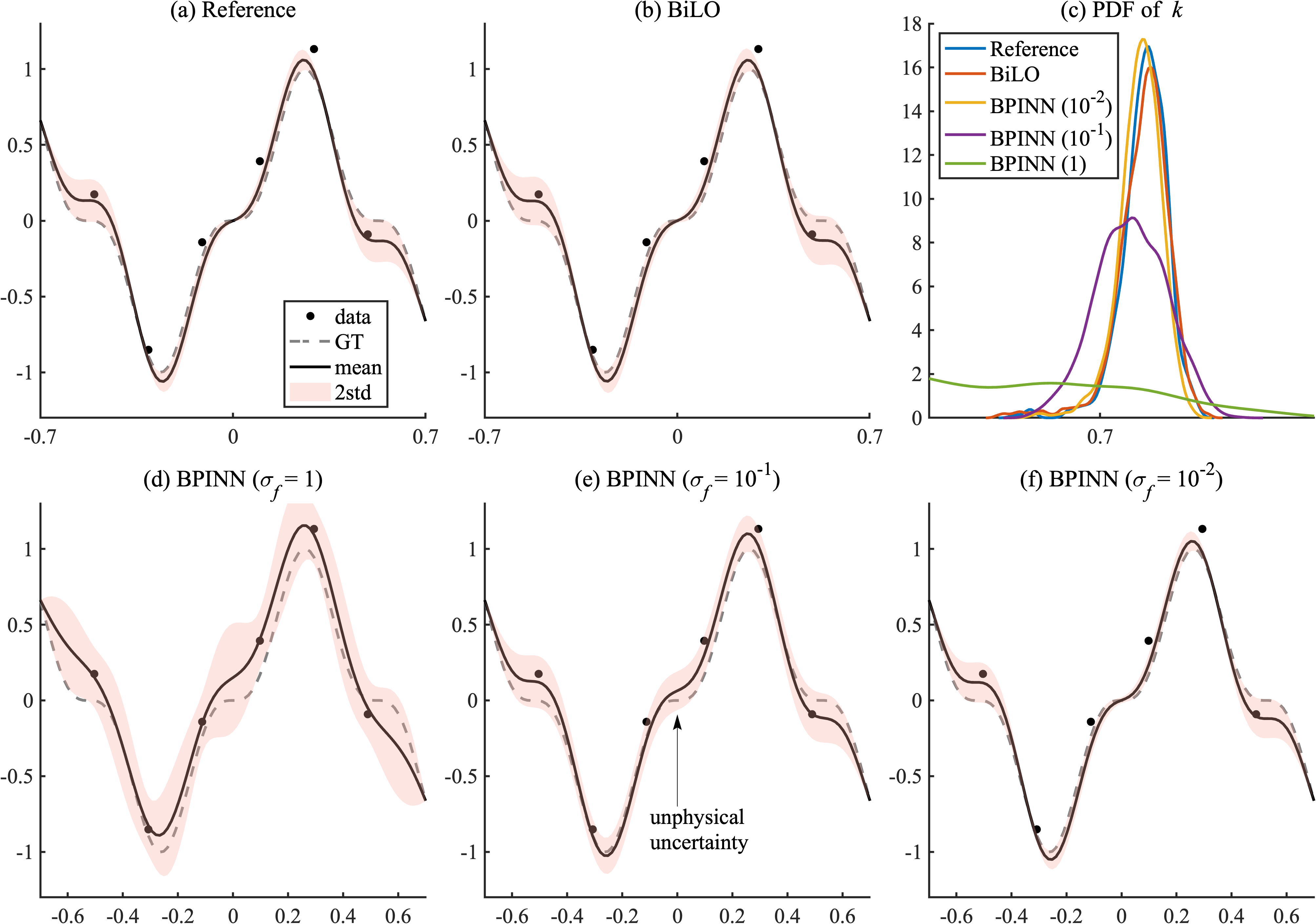
Figure 2: Inference results for the nonlinear Poisson problem. Noisy data, GT solution, mean and std of inferred $u$ using (a) Reference, (b) BiLO, (d-f) BPINN with varying $\sigma_{f}$. Panel (c) shows the probability density function (PDF) of inferred $k$. The soft PDE constraint of BPINN leads to unphysical uncertainty at $u(0)=0$ and larger uncertainty in $k$.

In Fig. 3, we compare the performance of BiLO and BPINN with $\sigma_{f}$ = 0.01 and 0.1 ($\sigma_{f}=1$ is not plotted due to its low accuracy for BPINN) under varying leapfrog step sizes $\delta t$ = $10^{-4}$, $10^{-3}$ and $10^{-2}$, with a fixed trajectory length $L=10$ for a fixed $N=5000$ (number of proposals). The effective sample size (ESS) [55] measures the number of independent samples in a Markov chain. Fig. 3(a) shows the acceptance rate, while Fig. 3(b) reports the ESS per wall time (in seconds), which reflects the overall efficiency of the sampler. In general, for fixed $L$, increasing $\delta t$ leads to longer trajectories and more decorrelated proposals, but also increases the risk of instability and rejection. As discussed in Sec. 2.6 and illustrated in Fig. 2, for BPINN, small $\sigma_{f}$ is required for accurate solution, but incurs a large computational cost as the step size $\delta t$ must be small to maintain stability. This is illustrated in Fig. 3 (a), where the acceptance rate of BPINN for fixed $\sigma_{f}$ drops significantly as $\delta t$ increases. Alternatively, for example, for fixed $\delta t=0.01$, reducing $\sigma_{f}$ from $0.1$ to $0.01$ leads to a dramatic drop in acceptance rate. For fixed $\delta t=0.1$, $\sigma_{f}=0.1$ has a near zero acceptance rate and $\sigma_{f}=0.01$ has zero acceptance rate.

In contrast, BiLO remains stable across a broad range of $\delta t$ and maintains high acceptance rates. This robustness arises from BiLO’s lower-dimensional sampling space, which avoids the high-dimensional weight space of neural networks and allows for efficient exploration of the space of the parameters with larger step sizes. By using larger $\delta t$ that is unattainable for BPINN with small $\sigma_{f}$, BiLO achieves higher ESS per wall time, as shown in Figure 3 (b).

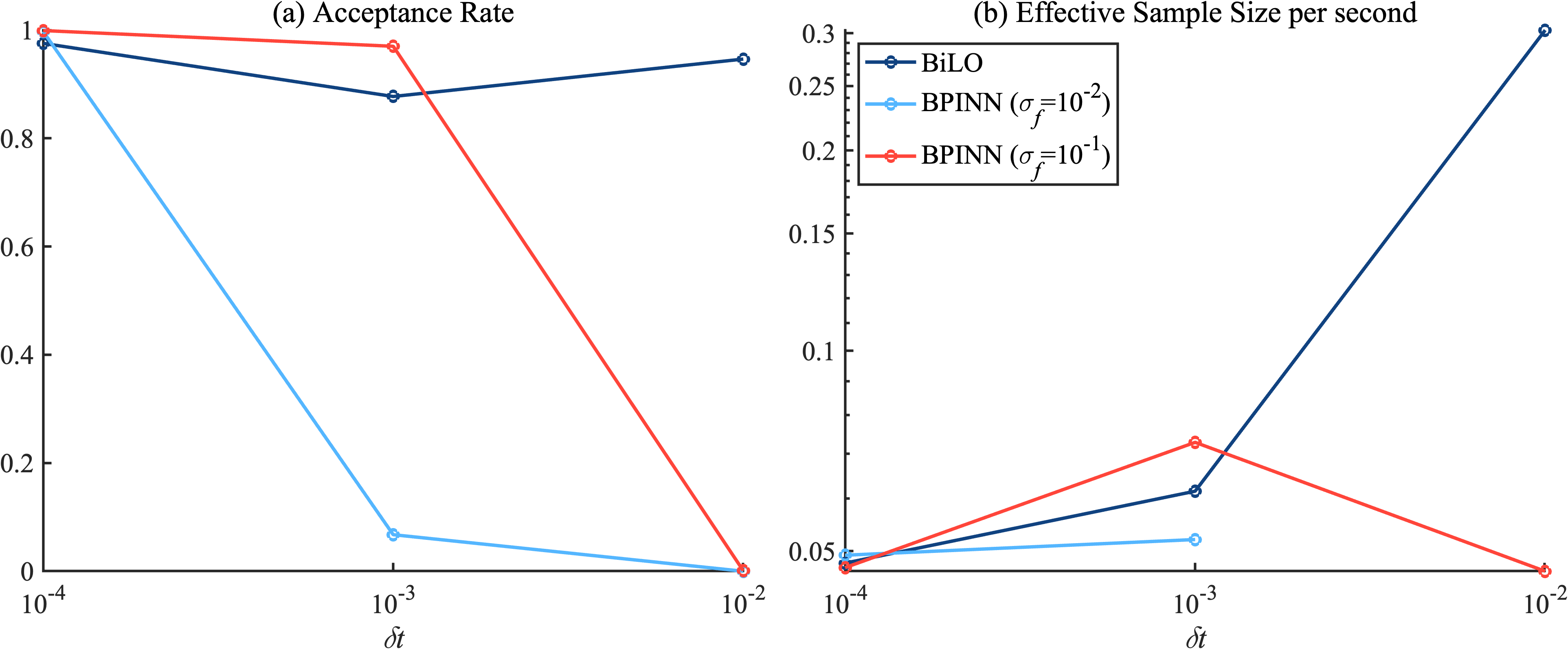
Figure 3: Sampling efficiency of BiLO and BPINN for the nonlinear Poisson problem under varying leapfrog step sizes $\delta t\in\{10^{-4},10^{-3},10^{-2}\}$ with fixed trajectory length $L$. (a) Acceptance rate. (b) Effective sample size (ESS) per second. BPINN is sensitive to both $\delta t$ and $\sigma_{f}$, with smaller $\sigma_{f}$ (stronger PDE constraint) requiring smaller $\delta t$ for numerical stability, leading to reduced acceptance and efficiency. In contrast, BiLO remains robust across all tested $\delta t$, benefiting from its lower-dimensional parameter space and achieving significantly higher sampling efficiency.

3.2 Inferring Stochastic Rates from Particle Data

We consider a problem motivated by inferring the dynamics of gene expression from static images of mRNA molecules in cells [56, 57]. The steady-state spatial distribution of these molecules can be modeled by the following boundary value problem with a singular source:

$$\frac{d^{2}u}{dx^{2}}+\lambda\delta(x-z)-\mu u=0,\quad u(0)=u(1)=0.$$ (20)

Here, the solution $u(x)$ represents the intensity of a spatial Poisson point process describing the locations of mRNA particles in a simplified 1D domain. The parameter $\lambda$ is the dimensionless birth rate (transcription) of mRNA at a specific gene site $z$, while $\mu$ is a a degradation rate, and the boundary condition describes export across the nuclear boundary.

Given $M$ snapshots of mRNA locations $\{q_{i}^{j}\}$ from different cells, the goal is to infer the kinetic parameters $\lambda$ and $\mu$. Since the particle locations follow a Poisson point process, we can construct a likelihood function directly from their positions. The resulting log-likelihood is [56]:

$$l(\lambda,\mu;q_{i}^{j})=M\int_{\Omega}u(x;\lambda,\mu)dx-\sum_{j=1}^{M}\sum_{i=1}^{N_{j}}\log u(q_{i}^{j};\lambda,\mu).$$

The data component of the potential energy $U(\theta)$ in our Bayesian framework (Eq. 4) is taken as the negative of this log-likelihood. This particular likelihood function, standard for spatial Poisson processes, consists of two terms: the sum of the log-intensity at each observed particle’s location and a term penalizing the total expected number of particles in the domain, $\int_{\Omega}u(x)dx$. The solution to the PDE is continuous, but its derivative is discontinuous at the source $z$; we handle this singularity using the cusp-capturing PINN [58]. The details are explained in Part I [10].

We use this example to show the effect of LoRA. In Fig. 4(a), we show the 90% highest posterior density region (HDPR) and the maximum a posteriori (MAP) of the inferred parameters $\lambda$ and $\mu$ using the reference method and BiLO with LoRA rank 2, rank 4, and Full FT. In Fig. 4(b), we show the ground truth (GT), prior distributions, and posterior distributions of $\lambda$ and $\mu$ (the ESS are around 150). Table 2 reports the relative error of the MAP estimates and the area of the 90% HDPR with respect to the reference. All methods yield less than 4% relative error across all three metrics. Across fine-tuning strategies, both $\lambda_{\rm MAP}$ and $\mu_{\rm MAP}$ are slightly overestimated relative to the reference, which can be attributed to the inexact PDE solution. The LoRA rank 2 and rank 4 results are comparable to Full FT, despite requiring significantly fewer trainable parameters. Minor differences between methods are likely due to variability from finite MCMC sampling.

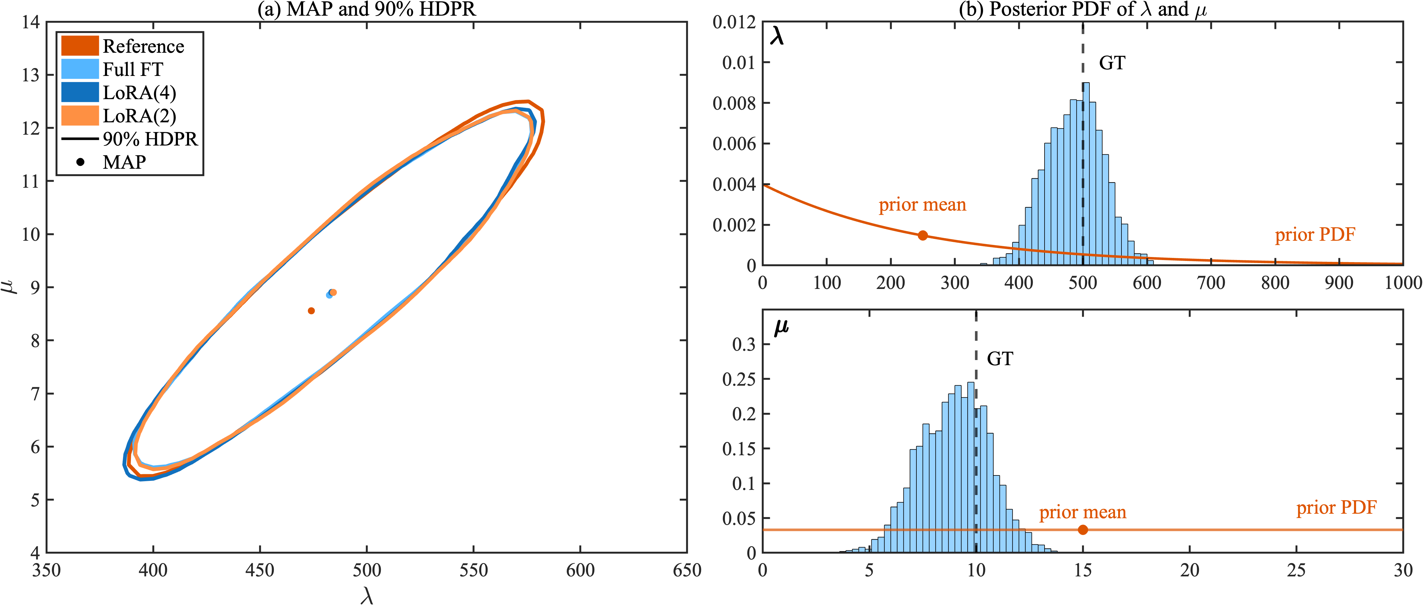
Figure 4: Inference of gene expression parameters $\lambda$ (birth rate) and $\mu$ (switch rate) using BiLO. (a): 90% highest density posterior region (HDPR) and maximum a posteriori (MAP) estimates obtained using BiLO with LoRA rank 2, rank 4, full FT, and reference. All results of BiLO are close to the reference solution. LoRA rank 2 and 4 yield comparable results to full FT. (b): Ground truth (GT), prior, and posterior distributions for $\lambda$ and $\mu$, with posterior sampled via BiLO using LoRA rank 2.

3.3 Darcy Flow Problem

We consider the following 2D Darcy flow problem on the unit square $\Omega=[0,1]\times[0,1]$:

$$\begin{cases}-\nabla\cdot(D(\mathbf{x})\nabla u)=f(\mathbf{x})&\text{in }\Omega\\ u=0&\text{on }\partial\Omega\end{cases}$$ (21)

where $f(\mathbf{x})=10$, $D(\mathbf{x})$ is unknown and needs to be inferred.

3.3.1 Inferring Unknown Functions

Here we briefly review the idea of inferring unknown functions in BiLO, as described in Part I (see Section 2.4 in [10]). Suppose the PDE depends on some unknown functions $f(\mathbf{x})$, such as the spatially varying diffusivity in a diffusion equation. Denote the PDE as

$$\mathcal{F}(D^{k}u(\mathbf{x}),...,Du(\mathbf{x}),u(\mathbf{x}),f(\mathbf{x}))=\mathbf{0}$$ (22)

We introduce an auxiliary variable $z=f(\mathbf{x})$, and we aim to find a local operator $u(\mathbf{x},z)$ such that $u(\mathbf{x},f(\mathbf{x}))$ solves the PDE locally at $f$. We introduce the augmented residual function, which has an auxiliary variable $z$:

$$a(\mathbf{x},z):=\mathcal{F}(D^{k}u(\mathbf{x},z),...,Du(\mathbf{x},z),u(\mathbf{x},z),z).$$ (23)

And the conditions for a local operator are:

1. $a(\mathbf{x},f(\mathbf{x}))=\mathbf{0}$

2. $\gradient_{z}a(\mathbf{x},z)|_{z=f(\mathbf{x})}=d_{z}\mathcal{F}(D^{k}u(\mathbf{x},z),...,Du(\mathbf{x},z),u(\mathbf{x},z),z)|_{z=f(\mathbf{x})}=\mathbf{0}$.

Condition 1 states that the function $u(\mathbf{x},f(\mathbf{x}))$ has zero residual, and condition 2 means that small perturbations of $f(\mathbf{x})$ do not change the residual, i.e., the PDE is satisfied locally at $f(\mathbf{x})$.

The unknown function $f$ can be represented by a Bayesian neural network [17, 24] or a Karhunen-Loève (KL) expansion [59, 21, 60]. We denote the parameterized function by $\theta$, where $\theta$ are the weights of the neural network or the coefficients of the KL expansion. In the following numerical example, we use a KL expansion to represent the unknown function $f(\mathbf{x})$, as the prior distribution can be more easily specified and it is easier to compute the reference solution.

3.3.2 Numerical Example

Let $g(\mathbf{x},\theta)$ be the 64 term KL expansion of a mean zero Gaussian process with covariance kernel $C=(-\Delta+\tau^{2})^{-d}$, where $\tau=3$ and $d=2$, and $-\Delta$ is the Laplacian on $\Omega$ subject to homogeneous Neumann boundary conditions [21, 60]:

$$g(\mathbf{x},\theta)=\sum_{i=1}^{8}\sum_{j=1}^{8}\theta_{ij}\sqrt{\lambda_{ij}}\cos(i\pi x_{1})\cos(j\pi x_{2}),\quad\lambda_{ij}=(\pi^{2}(i^{2}+j^{2})+\tau^{2})^{-2}$$ (24)

The prior of the KL coefficients is the standard normal distribution. The reference result is obtained by MH sampling with numerical solutions of the PDE computed on a 61$\times$61 grid. The initial guess for all simulations is $\mathbf{\theta}=\mathbf{0}$. In the example, we assume $D(\mathbf{x},\theta)=9s(20g(\mathbf{x},\theta))+3$, where $s(x)=1/(1+e^{-x})$ is the sigmoid function. This models a spatially varying diffusion coefficient with low and high diffusivity (3 and 12) in the domain. Noisy observations are collected at $21\times 21$ evenly spaced grid points, and the residual loss is evaluated at $61\times 61$ collocation points. The noise level is set to $\sigma_{d}=0.01$, corresponding to approximately 10% of the maximum value of the solution $u$.

Figure 5 illustrates the posterior inference of the spatially varying diffusion coefficient $D(\mathbf{x})$ in the 2D Darcy flow problem. Panel (a) shows the ground truth diffusion field, which serves as the target for inference. Panels (b) and (c) present the posterior means of $D(\mathbf{x})$ obtained using BiLO with LoRA rank 4 and the reference method, respectively, both of which capture the key spatial features of the true field. Panel (d) compares the uncertainty quantification along a fixed 1D slice of the domain, indicated by the dashed line in (a), by plotting the posterior mean and 95% confidence interval (mean $\pm$ two standard deviations) for both methods. Both the confidence interval and the posterior mean of BilO are close to the reference. The relative L2 error of the BiLO posterior mean with respect to the reference is 6.2%. The confidence interval from the reference and BiLO cover the ground truth with 96% and 92% probability, respectively.

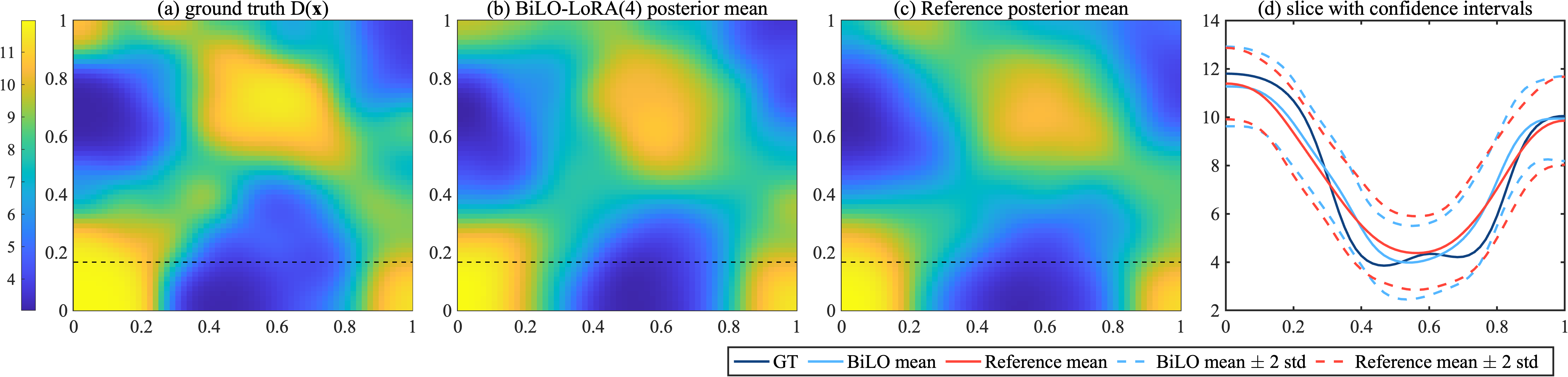
Figure 5: Posterior inference of the spatially varying diffusion coefficient $D(\mathbf{x})$ in the 2D Darcy flow problem. (a) The ground truth $D(\mathbf{x})$; (b) The posterior mean of $D(\mathbf{x})$ obtained using BiLO with LoRA rank 4; (c) The posterior mean of $D(\mathbf{x})$ obtained using Reference; and (d) The 95% confidence interval (mean $\pm$ 2 standard deviations) of the posterior evaluated along a 1D slice of the domain (dashed line in (a) (b) and (c)).

As discussed in 2.5, applying LoRA incurs a trade-off: while LoRA significantly reduces the number of trainable parameters, usually more iterations are needed to reach the same level of accuracy as the full FT (Algorithm 4). In addition, there is overhead in using LoRA, as the computational graph is more complicated. Figure 6 illustrates the computational trade-offs of using LoRA in BiLO. We fix the network depth at 6 and vary the width to control the overall model size. The $x$-axis in all subfigures represents the width of the neural network, where the number of parameters in the weight matrix $W$ scales quadratically with the width.

Fig. 6 (a) shows the average number of lower-level steps required to reach this tolerance. As the width increases, the model becomes more expressive, and fewer iterations are needed to reach convergence. Comparing LoRA (rank 4) with full FT, LoRA generally requires more iterations since it optimizes over a lower-dimensional subspace of the full parameter space. Fig. 6 (b) presents the average wall time per lower-level step. This increases with the number of trainable parameters. For large networks, LoRA significantly reduces per-step cost due to fewer trainable parameters. However, for small networks (e.g., width 512), the overhead of LoRA can make it slower than full FT, as the reduced number of parameters does not compensate for the additional complexity introduced by LoRA’s low-rank updates. Fig. 6 (c) reports the total wall time (in seconds) per upper-level step by multiplying the results from Figs. 6 (a) and (b). For small networks, full FT is more efficient. For large networks, LoRA offers a clear speed advantage, as its reduced per-step cost outweighs the modest increase in iteration count.

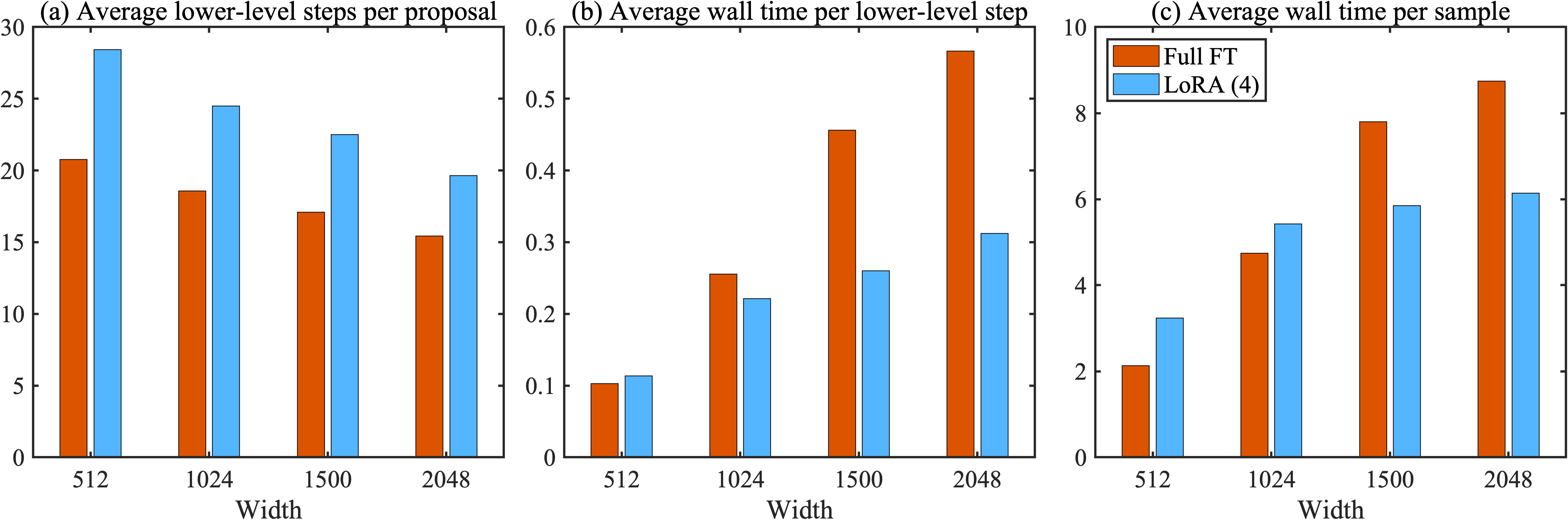
Figure 6: Computational trade-offs of LoRA (with $r=4$) and Full FT for the 2D Darcy flow problem, evaluated across neural networks of varying widths. (a) Average number of lower-level steps per proposal; (b) Average wall time (in seconds) per lower-level step. (c) Average wall time (in seconds) per sample, computed as the product of (a) and (b). For small networks (e.g., width 512), full FT is more efficient due to lower overhead. For larger networks, LoRA significantly reduces overall runtime by decreasing the number of trainable parameters.

4 Conclusion

In this paper, we have introduced a novel framework for efficiently solving Bayesian inverse problems constrained by PDEs by extending Bilevel Local Operator Learning (BiLO) with Low-Rank Adaptation (LoRA). Our approach enforces strong PDE constraints and integrates gradient-based MCMC methods, significantly enhancing computational efficiency and accuracy in parameter inference and uncertainty quantification. Through numerical experiments, we demonstrated that our method provides superior performance compared to Bayesian Physics-Informed Neural Networks (BPINNs). Notably, our approach avoids the computational challenges of directly sampling high-dimensional Bayesian neural network weights and mitigates issues arising from ill-conditioned PDE residual terms. Moreover, by incorporating LoRA, we substantially reduce computational overhead during the fine-tuning phase without compromising the accuracy or robustness of Bayesian inference. Our results on various problems, including nonlinear PDEs, singularly forced boundary value equations, and Darcy flow, highlight the effectiveness and scalability of our method.

A promising direction for future work is extending the BiLO framework to three-dimensional PDEs and inverse problems with high-dimensional parameter spaces, such as full-field identification problems in geophysics or medical imaging. Tackling these challenges will likely require integration with more efficient sampling algorithms, improved neural network architectures tailored to complex PDEs, and faster fine-tuning strategies to maintain scalability.

Code Availability

The code for the numerical experiments is available at https://github.com/Rayzhangzirui/BILO.

Appendix A Theoretical Analysis

We first briefly review the theoretical analysis of BiLO on the error of the upper-level gradient, introduced by the inexact minimization of the lower-level problem, which is presented in Part I [10].

Setup

Consider a bounded domain $\Omega\subset\mathbb{R}^{d}$. The PDE parameter $\theta\in\Theta\subset\mathbb{R}^{m}$. The weights $W\in\mathbb{R}^{n}$. The PDE residual operator $\mathcal{F}:H^{1}_{0}(\Omega)\times\Theta\to H^{-1}(\Omega)$. The PDE solution map (parameterized by weights $W$) $u:\Theta\times\mathbb{R}^{n}\to H^{1}_{0}(\Omega)$. The potential energy has the form $U[u,\theta]=\mathcal{J}[u]-\log P(\theta)$, where $\mathcal{J}[u]$ is the data-fit term and is a functional on the solution of the PDE, and $P(\theta)$ is the prior distribution of $\theta$. For simplicity, we also sometimes write $U(\theta,W)=U[u(\theta,W),\theta]$. The residual as a function of $\theta$ and $W$ is defined as

$$r(\theta,W):=\mathcal{F}(u(\theta,W),\theta)$$ (25)

Denote the (partial) Fréchet derivative of $\mathcal{F}$ by $\mathcal{F}_{u}$ and $\mathcal{F}_{\theta}$. The residual-gradient is given by

$$\nabla_{\theta}r(\theta,W):=\mathcal{F}_{u}(u(\theta,W),\theta)[\nabla_{\theta}u(\theta,W)]+\mathcal{F}_{\theta}(u(\theta,W),\theta)$$ (26)

The ideal optimal weights $W^{*}(\theta)$ satisfies the PDE for all $\theta$:

$$\mathcal{F}(u(\theta,W^{*}(\theta)),\theta)=0.$$

Its practical approximation is denoted by $\overline{W}$, which is obtained by terminating the optimization once the lower-level loss is within a specified tolerance,

$$\mathcal{L}_{\text{LO}}(\theta,\overline{W})\leq\epsilon.$$

We also denote $u^{*}=u(\theta,W^{*})$ the solution at the ideal optimal weights $W^{*}$, $\bar{u}=u(\theta,\overline{W})$ the solution at the approximate weights $\overline{W}$. We list the assumptions for the theoretical analysis, which are similar to those in Part I [10].

Assumption A.1 (Assumptions for Hypergradient Analysis).

Consider a parameterized PDE $\mathcal{F}(u,\theta)=0$ on a bounded domain $\Omega$ with $\theta\in\mathbb{R}^{m}$.

• Inexact Minimization: The lower-level optimization for the weights $\overline{W}$ terminates when the total local operator loss is within a tolerance $\epsilon$:

  $$\mathcal{L}_{\text{LO}}(\theta,\overline{W})=\norm{r(\theta,\overline{W})}_{L^{2}}^{2}+w_{\rm rgrad}\norm{\gradient_{\theta}r(\theta,\overline{W})}_{H^{-1}}^{2}\leq\epsilon.$$

  Since $w_{\rm rgrad}$ is some fixed weight, without loss of generality, we can assume that both the residual loss and the residual-gradient loss are controlled by $\epsilon$.

• PDE Operator Properties: The operator $F(u,\theta)$ are sufficiently Fréchet differentiable and stable, that is, if $\mathcal{F}(u,\theta)=0$ and $\norm{\mathcal{F}(v,\theta)}\leq\varepsilon$, then $\norm{v-u}\leq C\varepsilon$ for some constant $C$. The linearized operator at the $u$, denoted $\mathbf{L}_{u}[\cdot]:=F_{u}(u^{*},\theta)[\cdot]$, is stable, that is, if $\mathbf{L}_{u}[v]=f$, then $\norm{v}\leq C\norm{f}$ for some constant $C$.

• Smoothness: The data fitting term $\mathcal{J}$ is Lipschitz continuous. The parametrization $u$ is Lipschitz continuous in the weights $W$ and the parameters $\theta$ and has bounded derivatives with respect to $\theta$.

The approximate gradient of the potential energy is given by

$$g_{a}(\theta)=\nabla_{\theta}U(\theta,\overline{W})$$

And the true hypergradient is

$$g_{true}(\theta)=d_{\theta}U(\theta,W^{*}(\theta))$$

Since the prior $P(\theta)$ is independent of $W$, this difference arises solely from the data-fit term $\mathcal{J}$. As a direct consequence of Theorem 2 in Part I [10], we have the following result:

$$\norm{g_{a}(\theta)-g_{true}(\theta)}=O(\epsilon)$$

The preceding results bounds the dynamic error in the HMC sampler’s gradient. A separate and more fundamental issue is the static error in the sampler’s target distribution. Because the lower-level problem is solved inexactly, the algorithm targets an approximate posterior $\bar{\pi}$, which is computed using the approximate solution $\bar{u}$, instead of the ideal one $\pi_{*}$. The total error in the BiLO-HMC method thus has two distinct components: the dynamic sampler error (order $O(\epsilon)$) and this static target error. The following theorem isolates and bounds this static error.

Theorem A.1 (Posterior Perturbation Bound).

Under Assumption A.1, the KL divergence between the practical target posterior $\bar{\pi}(\theta)\propto\exp(-U(\theta,\overline{W}(\theta)))$ and the ideal posterior $\pi_{*}(\theta)\propto\exp(-U(\theta,W^{*}(\theta)))$ is order $O(\epsilon)$:

$$D_{\mathrm{KL}}\!\left(\bar{\pi}\;\big{\|}\;\pi_{*}\right)=O(\epsilon)$$

Proof.

Step 1: Bounding the potential difference. Let $\Delta U(\theta)=U(\theta,\overline{W}(\theta))-U(\theta,W^{*}(\theta))$. Since the prior $P(\theta)$ is independent of $W$, this difference arises solely from the data-fit term $\mathcal{J}$. Using the Lipschitz properties of $\mathcal{J}$ and the stability of the PDE,

$$|\Delta U|_{\infty}=\sup_{\theta\in\Theta}|\Delta U(\theta)| \leq K\norm{\bar{u}-u^{*}}=O(\epsilon)$$

Step 2: Bounding the KL divergence. The KL divergence is defined as

$$D_{\mathrm{KL}}\!\left(\bar{\pi}\;\big{\|}\;\pi_{*}\right)=\mathbb{E}_{\bar{\pi}}[\log(\bar{\pi}/\pi_{*})]=\log(Z_{*}/\bar{Z})-\mathbb{E}_{\bar{\pi}}[\Delta U].$$

The log-partition function ratio is bounded by

$$|\log(Z_{*}/\bar{Z})|=-|\log(\mathbb{E}_{\pi_{*}}[\exp(-\Delta U)])|\leq|\Delta U|_{\infty},$$

which follows from Jensen’s inequality. Therefore:

$$D_{\mathrm{KL}}\!\left(\bar{\pi}\;\big{\|}\;\pi_{*}\right) \leq|\log(Z_{*}/\bar{Z})|+|\mathbb{E}_{\bar{\pi}}[\Delta U]|$$

$$\leq 2|\Delta U|_{\infty}$$

$$=O(\epsilon)$$

∎

Appendix B Additional Results

B.1 Comparison with BPINN

For both BiLO and BPINN, we use 4-layer fully connected neural network with width 128, $\tanh$ activations. The model is trained using the Adam optimizer with AMSGrad, with a learning rate of $10^{-3}$ for the network weights. For leap-frog, we fix $L=10$ and cross validate $\delta t$. Residual loss is computed on 51 collocation points, and the noisy data is observed at 6 evenly spaced points in the domain.

	mean($k$)	std($k$)	std($u(0)$)
BPINN ($\sigma_{f}=1$)	0.517	0.173	$1.8\times 10^{-1}$
BPINN ($\sigma_{f}=10^{-1}$)	0.736	0.041	$6.3\times 10^{-2}$
BPINN ($\sigma_{f}=10^{-2}$)	0.746	0.025	$9.5\times 10^{-3}$
BiLO	0.753	0.026	$6.0\times 10^{-3}$
Reference	0.754	0.025	$5.0\times 10^{-15}$

Table 1: Comparison of the mean and standard deviation of $k$ and the standard deviation of $u(0)$ using different methods, the latter of which should be 0.

B.2 Inferring stochastic rates from particle data

For the experiments in this section, we use a 4-layer fully connected neural network with width 512 and $\tanh$ activations, augmented with random Fourier features [61]. The model is trained using the Adam optimizer [46] with AMSGrad [62], employing a learning rate of $10^{-4}$ for the network. We collect 5,000 HMC samples with $\delta t=10^{-2}$ and $L$ = 50, yielding ESS of approximately 150. The exact solution to the PDE (20) is given by [56]:

$$u(x)=\frac{\lambda}{\sqrt{\mu}}\csch(\sqrt{\mu})\sinh(\sqrt{\mu}\min\{x,z\})\sinh(\sqrt{\mu}(1-\max\{x,z\}))$$

We set $\epsilon=10$, which results in a relative error of approximately 1% in the infinity norm compared to the exact solution. The local operator loss is evaluated on 101 evenly spaced points in the domain. In this problem, the decay rate $\mu$ is typically on the order of $10$, while the birth rate $\lambda$ is on the order of several hundreds, as determined by the biological dynamics of the system. This scale ensures that a sufficient number of particles are present for inference. To improve numerical conditioning during training, we reparameterize $\lambda=100\bar{\lambda}$ and learn the rescaled parameter $\bar{\lambda}$. We also represent BiLO as $u(x,\theta;W)=m(x,\theta;W)^{2}x(1-x)$, where $m$ is the raw output of the MLP. This transformation enforces the boundary conditions $u(0)=u(1)=0$ and ensures $u\geq 0$, which is necessary for evaluating $\log u$ in the likelihood.

In Table 2, we show the relative error of the MAP estimate of $\lambda$ and $\mu$, and the area of 90% HDPR with respect to the reference method.

	Area	$\lambda_{\rm MAP}$	$\mu_{\rm MAP}$
Full FT	3.5%	1.8%	3.4%
LoRA rank 4	2.1%	2.0%	4.0%
LoRA rank 2	0.9%	2.2%	4.0%

Table 2: relative error of the MAP estimates of $\lambda$ and $\mu$ and the area of 90% HDPR with respect to the reference method

Appendix C Darcy Flow Problem

We set the lower-level optimization tolerance to $\epsilon=0.5$. The neural network follows a ResNet architecture [63], augmented with random Fourier features [61]. For the upper-level HMC sampler, we use $L=100$ leapfrog steps with step size $\delta t=10^{-3}$ and collect $N=5000$ samples. The BiLO model is represented as $u(\mathbf{x},z;W)=m(\mathbf{x},z;W)\mathbf{x}_{1}(1-\mathbf{x}_{1})\mathbf{x}_{2}(1-\mathbf{x}_{2})$, where $m$ is the raw output of the MLP and $z$ is the auxiliary variable. This form ensures that the Dirichlet boundary conditions are satisfied by construction.

References

- [1] C. Deng, S. Feng, H. Wang, X. Zhang, P. Jin, Y. Feng, Q. Zeng, Y. Chen, Y. Lin, OpenFWI: Large-Scale Multi-Structural Benchmark Datasets for Seismic Full Waveform Inversion (Jun. 2023). arXiv:2111.02926, doi:10.48550/arXiv.2111.02926.
- [2] J. Martin, L. C. Wilcox, C. Burstedde, O. Ghattas, A Stochastic Newton MCMC Method for Large-Scale Statistical Inverse Problems with Application to Seismic Inversion, SIAM Journal on Scientific Computing 34 (3) (2012) A1460–A1487. doi:10.1137/110845598.
- [3] Y. Yang, A. F. Gao, J. C. Castellanos, Z. E. Ross, K. Azizzadenesheli, R. W. Clayton, Seismic Wave Propagation and Inversion with Neural Operators, The Seismic Record 1 (3) (2021) 126–134. doi:10.1785/0320210026.
- [4] T. Bui-Thanh, C. Burstedde, O. Ghattas, J. Martin, G. Stadler, L. C. Wilcox, Extreme-scale UQ for Bayesian inverse problems governed by PDEs, in: SC ’12: Proceedings of the International Conference on High Performance Computing, Networking, Storage and Analysis, 2012, pp. 1–11. doi:10.1109/SC.2012.56.
- [5] J. Lipková, P. Angelikopoulos, S. Wu, E. Alberts, B. Wiestler, C. Diehl, C. Preibisch, T. Pyka, S. E. Combs, P. Hadjidoukas, K. Van Leemput, P. Koumoutsakos, J. Lowengrub, B. Menze, Personalized Radiotherapy Design for Glioblastoma: Integrating Mathematical Tumor Models, Multimodal Scans, and Bayesian Inference, IEEE Transactions on Medical Imaging 38 (8) (2019) 1875–1884. doi:10.1109/TMI.2019.2902044.
- [6] A. Chaudhuri, G. Pash, D. A. I. Hormuth, G. Lorenzo, M. Kapteyn, C. Wu, E. A. B. F. Lima, T. E. Yankeelov, K. Willcox, Predictive digital twin for optimizing patient-specific radiotherapy regimens under uncertainty in high-grade gliomas, Frontiers in Artificial Intelligence 6 (Oct. 2023). doi:10.3389/frai.2023.1222612.
- [7] M. K. Sen, P. L. Stoffa, Global Optimization Methods in Geophysical Inversion, Cambridge University Press, Cambridge, 2013. doi:10.1017/CBO9780511997570.
- [8] L. W. Cook, A. A. Mishra, J. P. Jarrett, K. E. Willcox, G. Iaccarino, Optimization under turbulence model uncertainty for aerospace design, Physics of Fluids 31 (10) (2019) 105111. doi:10.1063/1.5118785.
- [9] A. M. Stuart, Inverse problems: A Bayesian perspective, Acta Numerica 19 (2010) 451–559. doi:10.1017/S0962492910000061.
- [10] R. Z. Zhang, C. E. Miles, X. Xie, J. S. Lowengrub, BiLO: Bilevel Local Operator Learning for PDE Inverse Problems. Part I: PDE-Constrained Optimization (Jul. 2025). arXiv:2404.17789, doi:10.48550/arXiv.2404.17789.
- [11] M. Raissi, P. Perdikaris, G. E. Karniadakis, Physics-informed neural networks: A deep learning framework for solving forward and inverse problems involving nonlinear partial differential equations, Journal of Computational Physics 378 (2019) 686–707. doi:10.1016/j.jcp.2018.10.045.
- [12] Z. Li, N. Kovachki, K. Azizzadenesheli, B. Liu, K. Bhattacharya, A. Stuart, A. Anandkumar, Fourier Neural Operator for Parametric Partial Differential Equations (May 2021). arXiv:2010.08895, doi:10.48550/arXiv.2010.08895.
- [13] L. Lu, P. Jin, G. Pang, Z. Zhang, G. E. Karniadakis, Learning nonlinear operators via DeepONet based on the universal approximation theorem of operators, Nature Machine Intelligence 3 (3) (2021) 218–229. doi:10.1038/s42256-021-00302-5.
- [14] T. G. Grossmann, U. J. Komorowska, J. Latz, C.-B. Schönlieb, Can physics-informed neural networks beat the finite element method?, IMA Journal of Applied Mathematics 89 (1) (2024) 143–174. doi:10.1093/imamat/hxae011.
- [15] W. K. Hastings, Monte Carlo Sampling Methods Using Markov Chains and Their Applications, Biometrika 57 (1) (1970) 97–109. arXiv:2334940, doi:10.2307/2334940.
- [16] R. M. Neal, MCMC Using Hamiltonian Dynamics, 2011. arXiv:1206.1901, doi:10.1201/b10905.
- [17] R. M. Neal, Bayesian Learning for Neural Networks, Vol. 118 of Lecture Notes in Statistics, Springer, New York, NY, 1996. doi:10.1007/978-1-4612-0745-0.
- [18] M. Girolami, B. Calderhead, Riemann Manifold Langevin and Hamiltonian Monte Carlo Methods, Journal of the Royal Statistical Society Series B: Statistical Methodology 73 (2) (2011) 123–214. doi:10.1111/j.1467-9868.2010.00765.x.
- [19] A. Garbuno-Inigo, F. Hoffmann, W. Li, A. M. Stuart, Interacting Langevin Diffusions: Gradient Structure and Ensemble Kalman Sampler, SIAM Journal on Applied Dynamical Systems 19 (1) (2020) 412–441. doi:10.1137/19M1251655.
- [20] T. Bui-Thanh, M. Girolami, Solving large-scale PDE-constrained Bayesian inverse problems with Riemann manifold Hamiltonian Monte Carlo, Inverse Problems 30 (11) (2014) 114014. doi:10.1088/0266-5611/30/11/114014.
- [21] D. Z. Huang, J. Huang, S. Reich, A. M. Stuart, Efficient derivative-free Bayesian inference for large-scale inverse problems, Inverse Problems 38 (12) (2022) 125006. doi:10.1088/1361-6420/ac99fa.
- [22] D. Z. Huang, T. Schneider, A. M. Stuart, Iterated Kalman methodology for inverse problems, Journal of Computational Physics 463 (2022) 111262. doi:10.1016/j.jcp.2022.111262.
- [23] A. Pensoneault, X. Zhu, Efficient Bayesian Physics Informed Neural Networks for inverse problems via Ensemble Kalman Inversion, Journal of Computational Physics 508 (2024) 113006. doi:10.1016/j.jcp.2024.113006.
- [24] L. Yang, X. Meng, G. E. Karniadakis, B-PINNs: Bayesian physics-informed neural networks for forward and inverse PDE problems with noisy data, Journal of Computational Physics 425 (2021) 109913. doi:10.1016/j.jcp.2020.109913.
- [25] P. A. Guth, C. Schillings, S. Weissmann, Ensemble Kalman filter for neural network based one-shot inversion (Sep. 2020). arXiv:2005.02039, doi:10.48550/arXiv.2005.02039.
- [26] N. Kovachki, Z. Li, B. Liu, K. Azizzadenesheli, K. Bhattacharya, A. Stuart, A. Anandkumar, Neural Operator: Learning Maps Between Function Spaces (Oct. 2022). arXiv:2108.08481, doi:10.48550/arXiv.2108.08481.
- [27] J. Pathak, S. Subramanian, P. Harrington, S. Raja, A. Chattopadhyay, M. Mardani, T. Kurth, D. Hall, Z. Li, K. Azizzadenesheli, P. Hassanzadeh, K. Kashinath, A. Anandkumar, FourCastNet: A Global Data-driven High-resolution Weather Model using Adaptive Fourier Neural Operators (Feb. 2022). arXiv:2202.11214, doi:10.48550/arXiv.2202.11214.
- [28] L. Lu, R. Pestourie, S. G. Johnson, G. Romano, Multifidelity deep neural operators for efficient learning of partial differential equations with application to fast inverse design of nanoscale heat transport, Physical Review Research 4 (2) (2022) 023210. doi:10.1103/PhysRevResearch.4.023210.
- [29] S. Mao, R. Dong, L. Lu, K. M. Yi, S. Wang, P. Perdikaris, PPDONet: Deep Operator Networks for Fast Prediction of Steady-state Solutions in Disk–Planet Systems, The Astrophysical Journal Letters 950 (2) (2023) L12. doi:10.3847/2041-8213/acd77f.
- [30] Z. Li, H. Zheng, N. Kovachki, D. Jin, H. Chen, B. Liu, K. Azizzadenesheli, A. Anandkumar, Physics-Informed Neural Operator for Learning Partial Differential Equations, ACM / IMS Journal of Data Science 1 (3) (2024) 9:1–9:27. doi:10.1145/3648506.
- [31] C. White, J. Berner, J. Kossaifi, M. Elleithy, D. Pitt, D. Leibovici, Z. Li, K. Azizzadenesheli, A. Anandkumar, Physics-Informed Neural Operators with Exact Differentiation on Arbitrary Geometries, in: The Symbiosis of Deep Learning and Differential Equations III, 2023.
- [32] O. D. Akyildiz, M. Girolami, A. M. Stuart, A. Vadeboncoeur, Efficient Prior Calibration From Indirect Data (May 2025). arXiv:2405.17955, doi:10.48550/arXiv.2405.17955.
- [33] S. Wang, H. Wang, P. Perdikaris, Learning the solution operator of parametric partial differential equations with physics-informed DeepONets, Science Advances 7 (40) (2021) eabi8605. doi:10.1126/sciadv.abi8605.
- [34] L. Yang, S. Liu, T. Meng, S. J. Osher, In-context operator learning with data prompts for differential equation problems, Proceedings of the National Academy of Sciences 120 (39) (2023) e2310142120. doi:10.1073/pnas.2310142120.
- [35] T. O’Leary-Roseberry, P. Chen, U. Villa, O. Ghattas, Derivative-Informed Neural Operator: An efficient framework for high-dimensional parametric derivative learning, Journal of Computational Physics 496 (2024) 112555. doi:10.1016/j.jcp.2023.112555.
- [36] R. Molinaro, Y. Yang, B. Engquist, S. Mishra, Neural Inverse Operators for Solving PDE Inverse Problems (Jun. 2023). arXiv:2301.11167, doi:10.48550/arXiv.2301.11167.
- [37] L. Cao, T. O’Leary-Roseberry, P. K. Jha, J. T. Oden, O. Ghattas, Residual-based error correction for neural operator accelerated infinite-dimensional Bayesian inverse problems, Journal of Computational Physics 486 (2023) 112104. doi:10.1016/j.jcp.2023.112104.
- [38] E. J. Hu, Y. Shen, P. Wallis, Z. Allen-Zhu, Y. Li, S. Wang, L. Wang, W. Chen, LoRA: Low-Rank Adaptation of Large Language Models (Oct. 2021). arXiv:2106.09685, doi:10.48550/arXiv.2106.09685.
- [39] N. McGreivy, A. Hakim, Weak baselines and reporting biases lead to overoptimism in machine learning for fluid-related partial differential equations, Nature Machine Intelligence 6 (10) (2024) 1256–1269. doi:10.1038/s42256-024-00897-5.
- [40] S. Dong, N. Ni, A method for representing periodic functions and enforcing exactly periodic boundary conditions with deep neural networks, Journal of Computational Physics 435 (2021) 110242. doi:10.1016/j.jcp.2021.110242.
- [41] N. Sukumar, A. Srivastava, Exact imposition of boundary conditions with distance functions in physics-informed deep neural networks, Computer Methods in Applied Mechanics and Engineering 389 (2022) 114333. doi:10.1016/j.cma.2021.114333.
- [42] X. Glorot, Y. Bengio, Understanding the difficulty of training deep feedforward neural networks, in: Proceedings of the Thirteenth International Conference on Artificial Intelligence and Statistics, JMLR Workshop and Conference Proceedings, 2010, pp. 249–256.
- [43] M. D. Hoffman, A. Gelman, The No-U-Turn Sampler: Adaptively Setting Path Lengths in Hamiltonian Monte Carlo.
- [44] M. Hernández-Sánchez, F.-S. Kitaura, M. Ata, C. D. Vecchia, Higher Order Hamiltonian Monte Carlo Sampling for Cosmological Large-Scale Structure Analysis, Monthly Notices of the Royal Astronomical Society 502 (3) (2021) 3976–3992. arXiv:1911.02667, doi:10.1093/mnras/stab123.
- [45] T. Chen, E. B. Fox, C. Guestrin, Stochastic Gradient Hamiltonian Monte Carlo (May 2014). arXiv:1402.4102, doi:10.48550/arXiv.1402.4102.
- [46] D. P. Kingma, J. Ba, Adam: A Method for Stochastic Optimization (Jan. 2017). arXiv:1412.6980, doi:10.48550/arXiv.1412.6980.
- [47] A. S. Krishnapriyan, A. Gholami, S. Zhe, R. M. Kirby, M. W. Mahoney, Characterizing possible failure modes in physics-informed neural networks (Nov. 2021). arXiv:2109.01050, doi:10.48550/arXiv.2109.01050.
- [48] Q. Zhang, M. Chen, A. Bukharin, N. Karampatziakis, P. He, Y. Cheng, W. Chen, T. Zhao, AdaLoRA: Adaptive Budget Allocation for Parameter-Efficient Fine-Tuning (Dec. 2023). arXiv:2303.10512, doi:10.48550/arXiv.2303.10512.
- [49] S. Wang, L. Yu, J. Li, LoRA-GA: Low-Rank Adaptation with Gradient Approximation (Jul. 2024). arXiv:2407.05000, doi:10.48550/arXiv.2407.05000.
- [50] S. Hayou, N. Ghosh, B. Yu, LoRA+: Efficient Low Rank Adaptation of Large Models (Jul. 2024). arXiv:2402.12354, doi:10.48550/arXiv.2402.12354.
- [51] G. Chen, Y. He, Y. Hu, K. Yuan, B. Yuan, CE-LoRA: Computation-Efficient LoRA Fine-Tuning for Language Models (Feb. 2025). arXiv:2502.01378, doi:10.48550/arXiv.2502.01378.
- [52] D. Biderman, J. Portes, J. J. G. Ortiz, M. Paul, P. Greengard, C. Jennings, D. King, S. Havens, V. Chiley, J. Frankle, C. Blakeney, J. P. Cunningham, LoRA Learns Less and Forgets Less (Sep. 2024). arXiv:2405.09673, doi:10.48550/arXiv.2405.09673.
- [53] P. Rathore, W. Lei, Z. Frangella, L. Lu, M. Udell, Challenges in Training PINNs: A Loss Landscape Perspective (Jun. 2024). arXiv:2402.01868, doi:10.48550/arXiv.2402.01868.
- [54] G. O. Roberts, J. S. Rosenthal, Optimal scaling for various Metropolis-Hastings algorithms, Statistical Science 16 (4) (2001) 351–367. doi:10.1214/ss/1015346320.
- [55] S. Brooks, A. Gelman, G. Jones, X.-L. Meng, Handbook of Markov Chain Monte Carlo, CRC Press, 2011.
- [56] C. E. Miles, S. A. McKinley, F. Ding, R. B. Lehoucq, Inferring Stochastic Rates from Heterogeneous Snapshots of Particle Positions, Bulletin of Mathematical Biology 86 (6) (2024) 74. doi:10.1007/s11538-024-01301-4.
- [57] C. E. Miles, Incorporating spatial diffusion into models of bursty stochastic transcription, Journal of The Royal Society Interface 22 (225) (2025) 20240739. doi:10.1098/rsif.2024.0739.
- [58] Y.-H. Tseng, T.-S. Lin, W.-F. Hu, M.-C. Lai, A cusp-capturing PINN for elliptic interface problems, Journal of Computational Physics 491 (2023) 112359. doi:10.1016/j.jcp.2023.112359.
- [59] C. E. Rasmussen, C. K. I. Williams, Gaussian Processes for Machine Learning.
- [60] Z. Li, D. Z. Huang, B. Liu, A. Anandkumar, Fourier Neural Operator with Learned Deformations for PDEs on General Geometries (May 2024). arXiv:2207.05209, doi:10.5555/3648699.3649087.
- [61] S. Wang, H. Wang, P. Perdikaris, On the eigenvector bias of Fourier feature networks: From regression to solving multi-scale PDEs with physics-informed neural networks, Computer Methods in Applied Mechanics and Engineering 384 (2021) 113938. doi:10.1016/j.cma.2021.113938.
- [62] S. J. Reddi, S. Kale, S. Kumar, On the Convergence of Adam and Beyond (Apr. 2019). arXiv:1904.09237, doi:10.48550/arXiv.1904.09237.
- [63] K. He, X. Zhang, S. Ren, J. Sun, Deep Residual Learning for Image Recognition (Dec. 2015). arXiv:1512.03385, doi:10.48550/arXiv.1512.03385.