Quantitative Quantum Soundness for Bipartite Compiled Bell Games via the Sequential NPA Hierarchy

Abstract

Compiling Bell games under cryptographic assumptions replaces the need for physical separation, allowing nonlocality to be probed with a single untrusted device. While Kalai et al. (STOC’23) showed that this compilation preserves quantum advantages, its quantitative quantum soundness has remained an open problem. We address this gap with two primary contributions. First, we establish the first quantitative quantum soundness bounds for every bipartite compiled Bell game whose optimal quantum strategy is finite-dimensional: any polynomial-time prover’s score in the compiled game is negligibly close to the game’s ideal quantum value. More generally, for all bipartite games we show that the compiled score cannot significantly exceed the bounds given by a newly formalized sequential Navascués-Pironio-Acín (NPA) hierarchy. Second, we provide a full characterization of this sequential NPA hierarchy, establishing it as a robust numerical tool that is of independent interest. Finally, for games without finite-dimensional optimal strategies, we explore the necessity of NPA approximation error for quantitatively bounding their compiled scores, linking these considerations to the complexity conjecture $\mathrm{MIP}^{\mathrm{co}}=\mathrm{coRE}$ and open challenges such as quantum homomorphic encryption correctness for “weakly commuting” quantum registers.

1 Introduction

Since Bell’s groundbreaking work [Bel64], understanding and utilizing quantum nonlocality has been pivotal for both the conceptual foundations and practical applications of quantum theory. A central tool for probing nonlocality is the study of correlations arising from (nonlocal) Bell games [Bru+14], wherein multiple provers (also called players) coordinate their responses to questions chosen by a verifier (also called the referee). Quantum theory famously allows for correlations outside of classical theories, enabling quantum provers to sometimes achieve higher winning probabilities or “higher scores” than their classical counterparts.

The standard Bell game setup involves multiple, spatially separated provers who cannot communicate during the game, see Fig. 1.(a). This spatial separation is the typical way to enforce no-signaling constraints on the players or devices. However, verifying spatial separations between multiple untrusted quantum devices can be practically challenging. Moreover, from a theoretical standpoint, it is compelling to explore whether the power of quantum nonlocality can be verified and utilized using a single (untrusted) quantum device. A naive attempt to adapt a bipartite (Alice and Bob) Bell game to a single prover is as follows: the single prover receives Alice’s question $x$, computes her answer $a$, they subsequently receive Bob’s question $y$ and compute his answer $b$. However, here the prover has full information about Alice’s question (and answer) when deciding how to answer Bob’s question. This allows for coordination not permitted in the nonlocal case, and completely undermines the game’s no-communication assumption. To simulate the intended separation within a single device, the verifier must restrict information flow between the “Alice” and “Bob” rounds.

Homomorphic encryption (HE) offers a natural solution: the verifier can first encrypt Alice’s question into $\mathrm{Enc}_{sk}(x)$ using a secret key $sk$, and ask the prover to provide an encrypted answer $\mathrm{Enc}_{sk}(a)$. In HE the prover does not know the secret key, and therefore never has a decryption of $\mathrm{Enc}_{sk}(x)$ in their possession. Nonetheless, the HE satisfies a correctness functionality that enables the prover to compute an outcome $\alpha=\mathrm{Enc}_{sk}(a)$ as if they knew $x$, despite never being given $x$ in the plain (i.e., never given a decrypted $x$). The result is that, when Bob goes to make his computation based on $y$, it can no longer depend on $(x,a)$ in any meaningful way, as he only has access to their encryptions (Fig. 1.(c)). However, to allow for quantum strategies, conventional HE will not suffice, because the player strategies involve quantum computations and entanglement: the HE of Alice’s part of the strategy should not destroy her pre-shared entangled state with Bob. Therefore, we require a flavour of “quantum” HE which allows for the homomorphic evaluation of quantum circuits and satisfies a correctness with respect to auxiliary entangled systems functionality. Fortunately, constructions of quantum homomorphic encryption (QHE) schemes for polynomial size quantum circuits, with these additional properties, were established in [Bra18, Mah20], based on the (post-quantum) security of the learning with errors (LWE) problem. This approach was used by Kalai et al. [Kal+23], establishing the first compiled Bell games, where a multipartite Bell game can be transformed into an interactive protocol with a single quantum prover using a QHE scheme, at the cost of involving a number of rounds proportional to the number of parties. They demonstrated the classical soundness of such compilation, meaning that a cheating classical prover cannot exceed the classical score at the standard Bell game. Yet, an important issue was left open by their work: the quantum soundness, that is whether the compilation preserves the maximal quantum score.

More explicitly, the possibility of a dishonest quantum prover achieving scores for the compiled Bell game that significantly exceeded what was possible in the spatially separated Bell game was not ruled out. To date, this issue has been resolved in the negative for a number of cases like XOR and other simple Bell inequalities [NZ23, Cui+24, Bar+24, MPW24], such as the CHSH game [Cla+69]. For these games, it was shown that no efficient quantum prover could attain a winning probability negligibly (with respect to the encryption scheme’s security parameter $\lambda$) greater than the quantum value of the original game. Recently, some of us proved quantum soundness of all Bell games in the asymptotic limit of the security parameter going to infinity [Kul+25]. More precisely, we showed that for asymptotically large enough security parameter $\lambda$, the maximal quantum score at the compiled and standard Bell games is the same. Yet, this result is not quantitative, as it does not involve an explicit upper bound on the compiled score for security parameters $\lambda$. In particular, it does not inform a verifier of the security level needed to ensure the quantum provers’ behavior is suitably nonlocal, making this work unsuitable in practice.

In this work, we obtain quantitative quantum soundness bounds for all bipartite Bell games with finite-dimensional optimal quantum strategies, generalizing the results from [NZ23, Cui+24, Bar+24, MPW24, Kul+25]. More precisely, we show that the score a dishonest quantum prover can achieve at the compiled Bell game can explicitly be upper-bounded by a sequential variant of the Navascués-Pironio-Acín (NPA) hierarchy [NPA08, PNA10], which we also fully characterize in this work. With our result, the verifier can in practice bound the score of the dishonest prover by first computing a bound provided by this hierarchy, and then fixing the security parameter accordingly.

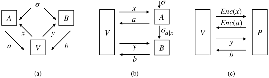
Figure 1: (a) Standard nonlocal Bell game: A verifier $V$ sends questions $x$ and $y$ to two spatially separated provers, Alice $A$ and Bob $B$, who reply with answers $a$ and $b$. For example, using quantum theory, the provers may pre-share a quantum state $\sigma$ to generate better answers. (b) Sequential Bell game: The verifier $V$ first send question $x$ to Alice and receive her answer $a$; subsequently, $V$ sends $y$ to Bob who replies with $b$. This protocol is said to satisfy the strongly no-signaling condition if $B$’s response is independent of $A$’s question $x$. In the quantum realization, $A$ first receives a state $\sigma$, measures and produce a post-measured state $\sigma_{a|x}$, and then forwards it to $B$, with condition $\sum_{a}\sigma_{a|x}=\sum_{a}\sigma_{a|x^{\prime}}$ for all $x,x^{\prime}$. (c) Compiled Bell game: The verifier $V$ interacts with a single prover $P$. The verifier first sends an encrypted question Enc$(x)$ and receives an encrypted answer Enc$(a)$, while the second message pair $y$ and $b$ is transmitted unencrypted. The QHE scheme chosen by the verifier enforces a form of computational no-signaling.

1.1 Nonlocal and compiled Bell games

Nonlocal Bell games. In nonlocal Bell games, a verifier interacts with multiple spatially separated provers, who are unable to communicate during the game. The provers receive questions from and provide answers to the verifier according to a pre-agreed protocol. The players win or lose based on a preset rule (see Fig. 1.(a)) determined by a winning function or predicate. The strategies that the provers adopt can be based on different resources available (e.g., classical or quantum), and the distinction between these theories is reflected in the corresponding Bell scores. The Bell score is the maximum winning probability using strategies permitted in a given resource or paradigm. For a given Bell game $\mathcal{G}$, we write $\omega_{\mathrm{qc}}(\mathcal{G})$ its optimal commuting quantum score and $\omega_{\mathrm{q}}(\mathcal{G})$ its optimal tensor product quantum score. More typically, the scores are compared in the classical and quantum cases. For example, in the CHSH game, the best classical Bell score is $0.75$, while the optimal quantum score is $\omega_{\mathrm{qc}}(\mathcal{G}_{\text{CHSH}})=\omega_{\mathrm{q}}(\mathcal{G}_{\text{CHSH}})=\cos^{2}(\pi/8)\approx 0.85$. This is often known as a game exhibiting quantum advantage.

Compiled Bell games. To transform from multi-prover to a setup with a single-prover, the authors of [Kal+23] introduce compiled Bell games $\mathcal{G}_{\mathrm{comp}}$, in which the no-communication constraint between the provers is replaced by a cryptographic one, using a QHE scheme. The QHE scheme used by the verifier is parameterized by a security parameter $\lambda$. For a chosen $\lambda$, the scheme is secure against $\mathrm{poly}(\lambda)$-runtime attacks from the prover. The verifier in the compiled game $\mathcal{G}_{\mathrm{comp}}$ sends an encrypted question $x$ and receives the encrypted answer $a$ back from the prover. The verifier then sends $y$ and receives $b$ (see Fig. 1.(c)). Encryption is not required in the second round because the information is of no use later in the game. In this setting, the prover’s strategies for the compiled game are characterized by quantum polynomial time (QPT) circuits, denoted $S$, which upon obtaining $x$ produce the outcome $a$. The winning probability of employing strategy $S$ in the game $\mathcal{G}_{\mathrm{comp}}$ (with security parameter $\lambda$) is the compiled Bell score $\omega_{\lambda}({\mathcal{G}_{\mathrm{comp}},S})$. This compilation procedure guarantees classical soundness. That is, no dishonest classical prover can exceed the maximal classical winning probability in the no communication setting. Furthermore, by the features of the QHE scheme, quantum completeness is also guaranteed. That is, an honest quantum prover can achieve the optimal quantum score in the nonlocal case [Kal+23].

Establishing quantum soundness of $\omega_{\lambda}({\mathcal{G}_{\mathrm{comp}},S})$ (i.e., that no dishonest quantum prover can exceed the maximal quantum score more than some quantitatively negligible function in $\lambda$) remains open. Recently, operator-algebraic techniques [Kul+25] provided qualitative insights into this quantum compiled value in the asymptotic limit of the security parameter ($\lambda\to\infty$). Their approach uses the fact that in the limit, compiled strategies correspond to strategies for sequential Bell games satisfying the strongly non-signaling property (see Fig. 1.(b)). These quantum strategies for sequential Bell games turn out to be equivalent to the commuting quantum strategies [HJW93, Kul+25], and so it follows that as $\lambda\to\infty$, the scores $\omega_{\lambda}({\mathcal{G}_{\mathrm{comp}},S})$ achievable by any QPT strategy $S$ converge to the quantum commuting score $\omega_{\mathrm{qc}}(\mathcal{G})$.

Yet, this last result is only qualitative: in practice, the verifier can only take finite $\lambda$, in which case [Kul+25] provides no concrete bound on the score $\omega_{\lambda}({\mathcal{G}_{\mathrm{comp}},S})$ the cheating prover can obtain, as it does not provide a quantitative bound on how quickly these compiled scores converge for finite $\lambda$. Therefore, the quantitative quantum soundness of all compiled Bell games as proposed in [Kul+25] remains an open problem. This is the main challenge that our work addresses.

1.2 Main results

Our work has two primary contributions. (i) We give the first quantitative quantum soundness bounds for every bipartite compiled Bell game whose optimal quantum strategies are finite-dimensional, showing that the compiled score is provably close to the game’s ideal quantum score. In fact, for all bipartite compiled Bell games, we obtain upper bounds for the compiled scores in terms of the sequential NPA hierarchy. (ii) We formalize and fully characterize a sequential variant of the NPA hierarchy, a tool that underpins our analysis and is of independent interest. In the following, we give more details.

Quantitative bound for bipartite compiled Bell scores. Let $\mathcal{G}$ be any bipartite Bell game and $\mathcal{G}_{\mathrm{comp}}$ its compiled version. Our first main result upper-bounds the score $\omega_{\mathrm{comp}}^{\lambda}(\mathcal{G}_{\mathrm{comp}},S)$ achievable by any QPT strategy $S$ as the ideal commuting-operator score $\omega_{\mathrm{qc}}(\mathcal{G})$ plus two error terms: an approximation term $\varepsilon(n)$ arising from level $n$ of the sequential NPA hierarchy and a negligible cryptographic term (from the QHE scheme and the implementation of $S$). When $\mathcal{G}$ admits a finite-dimensional optimal strategy, the hierarchy has a feasible solution at some finite level $n_{0}$, so $\varepsilon(n_{0})=0$ and we obtain a negligible gap to the tensor-product quantum value. The precise statement is as follows.

Theorem A (Theorems 2.7 and 2.8).

Consider any bipartite Bell game $\mathcal{G}$ with commuting quantum score $\omega_{\mathrm{qc}}(\mathcal{G})$. Then, for any QPT strategy $S$, its achievable score $\omega_{\lambda}({\mathcal{G}_{\mathrm{comp}},S})$ is bounded as

$$\omega_{\lambda}({\mathcal{G}_{\mathrm{comp}},S})\leq\omega_{\mathrm{qc}}(\mathcal{G})+\varepsilon(n)+\mathrm{negl}_{S,n}(\lambda),$$

where $\varepsilon(n):=\omega_{\mathrm{seqNPA}}^{n}(\mathcal{G})-\omega_{\mathrm{qc}}(\mathcal{G})$ is the approximation error from the $n$-th level of the sequential NPA hierarchy, which monotonically vanishes as $n\to\infty$. The term $\mathrm{negl}_{S,n}(\lambda)$ is a negligible function (dependent on the QHE scheme, strategy $S$, and level $n$) that vanishes faster than any polynomial in $\lambda$.

Furthermore, if $\mathcal{G}$ admits a finite-dimensional optimal quantum strategy (i.e., the optimal quantum correlations lie in $C_{q}$), then

$$\omega_{\lambda}({\mathcal{G}_{\mathrm{comp}},S})\leq\omega_{\mathrm{q}}(\mathcal{G})+\mathrm{negl}_{S}(\lambda),$$

where $\omega_{\mathrm{q}}(\mathcal{G})$ is the optimal tensor product quantum score and $\mathrm{negl}(\lambda)$ is some negligible function depending only on the QHE scheme and the strategy $S$.

Hence, knowing the approximation error of the sequential NPA hierarchy $\varepsilon(n)$ for a game $\mathcal{G}$ provides a quantitative upper bound on the maximal score that a dishonest prover can obtain at the compiled game $\mathcal{G}_{\mathrm{comp}}$ with some QPT strategy $S$. By letting $n,\lambda\to\infty$, we recover the asymptotic quantum soundness result of [Kul+25]. In addition, for all bipartite Bell games with optimal finite-dimensional strategies, the second inequality establishes the quantitative quantum soundness of its compiled version, which is a generalization to [NZ23, Cui+24, Bar+24, MPW24].

While the problem of deciding if a correlation admits a finite-dimensional quantum realization is undecidable in general [FMS25], many of the most studied Bell games are known to have finite-dimensional optimal strategies. Note also that an infinite-dimensional quantum strategy poses several issues. First, it is unclear how to implement such a strategy efficiently with polynomial-size circuits. Second, even if one could engineer such an implementation, compiling it while preserving its score would require a justification of the correctness of the QHE scheme in the infinite-dimensional setting.

The sequential Navascués-Pironio-Acín hierarchy. As a second main result, we formally introduce and characterize the sequential NPA hierarchy (Section 3), which underpins our quantitative soundness proof. While its asymptotic convergence to the commuting score was established in [Kul+25], we provide a concrete definition (Eq. 21) and a comprehensive characterization of its properties. One characterization that is crucial to A is the following stopping criterion based on the flatness condition (Definition 3.2), also known as the rank-loop:

Theorem B (Theorem 3.3).

A bipartite Bell game $\mathcal{G}$ admits a finite-dimensional optimal quantum strategy if and only if there exists a flat optimal solution to the sequential NPA hierarchy for $\mathcal{G}$ at some finite level $n$.

In addition, we:

1. Establish its precise relationship to the standard NPA hierarchy at any finite level $n$. In Proposition 3.1, we prove that the sequential NPA hierarchy is equivalent to a relaxed version of the standard NPA hierarchy where Alice’s operators only appear to satisfy POVM completeness from Bob’s perspective (Eq. 23). This result implies that this relaxed hierarchy also converges to the quantum commuting score.

2. Identify (via Proposition 3.5) its conic dual with the sparse sum of squares (SOS) hierarchy (Eq. 25) [KMP22]. This duality not only provides a complete theoretical picture but also connects our hierarchy to existing numerical examples [MW23, Chapter 6.7].

1.3 Methods, techniques and further results

Our results rely on a combination of existing tools adapted to the compiled game setting and novel techniques developed in this work, which may be of independent interest. Key elements include:

1. Navascués-Pironio-Acín hierarchy and its generalizations. The standard NPA hierarchy [NPA08, PNA10] provides a systematic method, based on semidefinite programming (SDP), to compute upper bounds on the commuting quantum score $\omega_{\mathrm{qc}}(\mathcal{G})$. It involves a sequence of SDP relaxations indexed by an integer level $n$, yielding monotonically decreasing upper bounds $\omega_{\mathrm{NPA}}^{n}(\mathcal{G})$ that converge to $\omega_{\mathrm{qc}}(\mathcal{G})$. It generalizes the Lasserre-Parrilo hierarchy [Las01, Par03] to non-commutative settings.

   As discussed in the previous subsection, to establish our quantitative bound on $\omega_{\lambda}({\mathcal{G}_{\mathrm{comp}},S})$ (A), we consider a sequential generalization of the standard NPA hierarchy, which we introduce and fully characterize (Section 3).

2. Imperfect finite-dimensional quantum representations via flat extension. To connect finite levels of the (sequential) NPA hierarchy to concrete quantum representations, we consider the flat extension method [HKM12], central to the discussion in  Sections 2.2 and 2.3, and pivotal in the proof of B, Propositions 3.1 and 4.1. Given the moment matrix from a finite level $n$ solution of the NPA hierarchy, the flat extension technique gives positive linear functionals and, via the GNS construction, a representation of the associated finite-dimensional quantum strategy that exactly satisfies all algebraic constraints imposed by that $n$-th NPA level.

   Notably, while these extracted strategies faithfully realize the $n$-th level NPA model, the constraints of this finite level are generally weaker than those of an ideal commuting quantum strategy. For instance, the $n$-th level NPA hierarchy enforces that certain polynomial expressions involving commutators evaluate to zero, as they would for truly commuting operators. I.e., $\mathop{}\!\mathrm{Tr}{\left(\rho[A_{a|x},B_{b|y}]P\right)}=0$ for all polynomials $P$ of degrees $\leq 2n-2$. However, it does not, in general, enforce the operator identity $[A_{a|x},B_{b|y}]=0$.

   Consequently, the strategies obtained via flat extension from a finite NPA level are “imperfect” in the sense that Alice’s and Bob’s operators might not strictly commute with each other, even though all $n$-th level NPA conditions (including those partial commutativity constraints and linear constraints like POVMs summing to identity) are met. This technique thus provides a concrete way to construct operational (albeit imperfect) quantum representations from a finite level of the NPA hierarchy.

   It is worth noting that the authors of [CV15] presented an alternative construction of almost commuting strategies from the NPA hierarchy. While our flat extension-based method produces strategies satisfying exact commutation when tested against low-degree polynomials their approach yields strategies whose commutators are controlled in operator norm, with a bound scaling as $O(1/\sqrt{n})$ for the $n$-th NPA level. This is achieved by analyzing the projections onto low-degree subspaces of the original NPA solution, rather than by constructing a new representation from a modified moment matrix.

3. Isolating signaling effect using symmetric group representation theory. A key observation from [Kul+25] is that every QPT strategy of compiled Bell games at security parameter $\lambda$ implicitly contains a negligible amount of signaling (permitted by the QHE scheme) from the protocol’s encrypted part to the unencrypted part with $\mathrm{poly}(\lambda)$-size circuits.

   Therefore, analyzing this weak signaling effect and its impact on the compiled Bell score is interesting. To this end, inspired by [Ren+17], we utilize representation theory of the symmetric group to develop a technique for decomposing the operators that do not satisfy the ideal no-signaling conditions (Proposition 2.6). This method allows us to systematically decompose these operators into components corresponding to a no-signaling part, a signaling part, and a residual (positive) term. This decomposition is central to establish our main theorem (A), since it allows us to identify the no-signaling part to the sequential NPA hierarchy at a fixed level, while the signaling part and the residual term can both be bounded by the negligible functions from the cryptographic assumption. Observe that, since this decomposition technique is formulated rather generally, it may also be useful for isolating and analyzing signaling effects in other quantum protocols.

4. Almost-commuting strategies from computationally hard Bell games. Tsirelson’s theorem [SW08] shows that the correlations attainable from any finite-dimensional genuinely commuting quantum strategies can be also obtained from tensor product quantum strategies (i.e., those in $C_{qa}$). More recently, the approximate Tsirelson’s theorems [XRK25] investigate the situation when the finite-dimensional quantum strategy is only approximately commuting and provide operator norm bounds for quantifying its “distance” to tensor product quantum strategies. We argue that computational complexity arguments reveal this distance must be non-negligible for certain hard Bell games.

   Specifically, the $\mathrm{MIP}^{\mathrm{co}}=\mathrm{coRE}$ conjecture (see e.g., [Ji+21]), via Propositions 4.1 and 4.3, implies the existence of $\mathrm{coRE}$-hard games where almost-commuting strategies achieve scores significantly exceeding $\omega_{\mathrm{qc}}(\mathcal{G})$. For these almost-commuting strategies, the “distance” to any $C_{qa}$ strategy, as per [XRK25], must be non-negligible to avoid contradicting this score advantage. This implies these strategies generate correlations fundamentally distinct from $C_{qa}$.

   This insight is complemented by the established $\mathrm{MIP}^{*}=\mathrm{RE}$ result [Ji+21]. For $\mathrm{RE}$-hard games, if near-optimal almost-commuting strategies (e.g., from NPA truncation) could be approximated by $C_{qa}$ strategies with arbitrarily small error (i.e., negligible “distance”), it would contradict the known separation between sets $C_{qa}$ and quantum commuting observable set $C_{qc}$. Thus, for these games too, such almost-commuting strategies must be non-negligibly distant from any in $C_{qa}$.

   In both cases, these non-negligible distances highlight that the high-scoring almost-commuting strategies are fundamentally distinct from any commuting tensor-product strategy.

1.4 Open problems and outlook

Building on our results, several important open questions for future research emerge:

1. Necessity of NPA approximation errors and QHE correctness for almost-commuting strategies: A key question arising from our work is whether the game-specific NPA approximation error $\varepsilon(n)$ is fundamentally necessary for quantitative quantum soundness to games $\mathcal{G}$ without a finite-dimensional optimal quantum strategy. In Section 4, we explore a potential argument supporting this necessity.

   Our investigation, based on the standard complexity conjecture $\mathrm{MIP}^{\mathrm{co}}=\mathrm{coRE}$ (4.2), suggests the existence of Bell games $\mathcal{G}^{(n)}$ for which the $n$-th level NPA score (and hence also the sequential NPA score) significantly exceeds the true commuting quantum value (Proposition 4.3), implying that no universal NPA approximation error can exist for the NPA hierarchy. Notably, if the conjecture $\mathrm{MIP}^{\mathrm{co}}=\mathrm{coRE}$ is false, then there is a universal NPA approximation error and our quantitative quantum soundness results applies to all bipartite Bell games. On the other hand, if the conjecture does hold, we provide constructions for almost-commuting quantum strategies and weakly-signaling sequential quantum strategies that achieve these high NPA scores (Proposition 4.1).

   Consequently, it is likely that one can construct a compiled Bell game out of the family $(\mathcal{G}^{(n)})$ and compile the associated high-scoring strategies into a cheating QPT strategies. This would imply the necessity of the game specific NPA approximation error for quantitative quantum soundness. However, as we discuss in Section 4.2, several significant obstacles prevent the straightforward compilation of these high-scoring strategies. These challenges include: (1) finding potentially more efficient constructions of the high-scoring strategies; (2) determining the scaling of the game size for the family $(\mathcal{G}^{(n)})$, which depends on the potential proof of $\mathrm{MIP}^{\mathrm{co}}=\mathrm{coRE}$; and critically, (3) formulating and justifying a more general QHE assumption suitable for almost-commuting scenarios, i.e., “correctness with auxiliary input for weakly commuting registers.” Resolving these challenges is crucial to definitively establish the role of game-specific NPA approximation errors in quantitative quantum soundness.

2. Separation between sequential and standard NPA hierarchies: We introduced the sequential NPA hierarchy and showed it is equivalent to the standard NPA hierarchy at finite levels with relaxed POVM completeness constraints. We also characterized its stopping criteria and identified conic dual with the sparse SOS hierarchy [KMP22, MW23]. An interesting question is whether there exist Bell games $\mathcal{G}$ for which the sequential NPA hierarchy $\omega_{\mathrm{seqNPA}}^{n}(\mathcal{G})$ converges much slower to $\omega_{\mathrm{qc}}(\mathcal{G})$ than the standard NPA hierarchy $\omega_{\mathrm{NPA}}^{n}(\mathcal{G})$. Finding such explicit separations (which we conjecture exist considering the numerical analysis on $I_{3322}$ of the sparse SOS hierarchy [MW23, Chapter 6.7]) would provide deeper insights into the convergence properties of these hierarchies and the precise implications of using Arveson’s Radon-Nikodym derivatives [Arv69] in the sequential formulation.

3. Generalization to robust self-testing for compiled games: Robust self-testing allows characterizing a quantum device based solely on observed correlations, even with experimental imperfections. While the exact self-testing result of compiled Bell games in the asymptotic limit of the security parameter is established [Kul+25, Theorem 6.5], the question of whether one can generalize this to the robust case in the non-asymptotic setup remains open. We explore into this direction in Section 2.6, and note on the need to extend the notion of robust self-testing beyond quantum strategies to cover “quasi-quantum” or imperfectly realized strategies, possibly using results similar to [XRK25].

4. Quantum soundness of multipartite compiled Bell games beyond two parties: Current investigations into quantum soundness, including our own, have primarily focused on the compilation of bipartite Bell games. Extending quantitative quantum soundness results to games with three or more provers is the natural next step, but it presents a significant challenge: it requires a sophisticated generalization of operator-algebraic tools, namely for Arveson’s Radon-Nikodym derivatives [Arv69].

   In concurrent work, the authors of [Bar+25] address this very issue, establishing asymptotic quantum soundness for all multipartite games by proving a new chain rule for these derivatives. Their multipartite framework is complementary to our methods, and we believe merging their techniques with ours provides a clear path toward a quantitative quantum soundness analysis for multipartite compiled games.

5. Exploring almost commuting correlations: The almost commuting strategies arising from $\mathrm{coRE}$-hard games (Propositions 4.1 and 4.3) are necessarily “far” from any finite-dimensional tensor-product strategies. The behavior of such strategies was characterized from an asymptotic perspective by Ozawa [Oza13], who showed that as commutators vanish, the resulting correlations converge to the commuting set $C_{qc}$. More recently, quantitative bounds have been developed to measure the distance from an almost-commuting correlation to the sets $C_{qa}$ and $C_{qc}$ [XRK25]. These works provide tools for exploring the structure of the set of almost commuting correlations. This investigation, in additional to foundational interests, is also practically motivated since enforcing strict commutation can be challenging due to experimental limitations.

6. Bigger picture—from space-like separated provers to single compiled provers: A compelling direction in quantum information involves replacing the requirement of space-like separation in Bell game-based protocols with computational or cryptographic assumptions on a single quantum device. Beyond the research on compiled Bell games already discussed, recent works have also advanced our understanding of nonlocality under computational assumptions [Glu+24], as well as applications in self-testing [MV21] and device-independent quantum key distribution [Met+21] in the single-prover paradigm.

   Our work contributes to this broader effort by providing quantitative soundness bounds for all bipartite compiled Bell games. More fundamentally, the operator algebraic techniques we employ offer a direct bridge between the “space-like separation world” and the “compiled single-prover world,” suggesting the potential for a unified mathematical framework. Such a framework could systematically translate protocols originally designed for spatially separated parties into equivalent single-prover protocols with cryptographic assumptions, all while quantitatively preserving their essential properties (such as achievable scores).

1.5 Structure of the paper

The remainder of this paper is organized as follows. In Section 2, we establish quantitative upper bounds for the quantum scores of compiled Bell games. More specifically, Section 2.1 introduces compiled Bell games in the context of the sequential NPA hierarchy at level $n$ and the associated relaxed no-signaling conditions. Section 2.2 details the flat extension technique, crucial for extending positive linear maps defined on subspaces of operators to positive linear functionals on the full algebra. Building on this, Section 2.3 constructs a quantum representation for these compiled Bell games from the extended functionals. A key technical contribution is presented in Section 2.4, where we develop a method to decompose Alice’s operators into signaling and no-signaling components, allowing us to bound the signaling advantage. Section 2.5 then combines these elements to present the main quantitative soundness theorems, relating the compiled game scores to the sequential NPA hierarchy and the quantum scores. Finally, Section 2.6 briefly discusses potential notions and challenges for robust self-testing in the context of compiled Bell games.

In Section 3, we formally introduce and analyze the sequential NPA hierarchy (Eq. 21). In particular, Section 3.1 compares this hierarchy to the standard NPA hierarchy, particularly at finite levels where the sequential version is equivalent to the standard NPA hierarchy with a relaxed POVM completeness condition. In Section 3.2 we fully describe and prove the stopping criteria of the sequential NPA hierarchy. Finally, Section 3.3 further characterizes the sequential NPA hierarchy by identifying its conic dual as a special case of the sparse sum of squares (SOS) hierarchy.

Section 4 explores arguments suggesting that game-specific NPA approximation errors are essential for establishing quantitative quantum soundness in compiled Bell games. Section 4.1 first details the construction of explicit almost-commuting quantum strategies and their weakly signaling sequential counterparts, which achieve the $n$-th level NPA score for any given Bell game $\mathcal{G}$. Then, Section 4.2 uses the standard hardness conjecture $\mathrm{MIP}^{\mathrm{co}}=\mathrm{coRE}$ (4.2) to argue for the existence of a family of Bell games $\mathcal{G}^{(n)}$ where the $n$-th level NPA score significantly exceeds the true quantum commuting score. This section proceeds to define a compiled Bell game based on this family, $\mathcal{G}_{\mathrm{comp}}=(\mathcal{G}^{(n(\lambda))}_{\mathrm{comp}})_{\lambda}$, and discusses the substantial challenges in compiling the aforementioned high-scoring strategies into a single QPT strategy $(S^{(\lambda)}_{\mathrm{comp}})$ for this compiled game. Successfully overcoming these challenges would demonstrate the necessity of incorporating NPA approximation errors for robust quantitative soundness.

2 Quantitative bounds for the compiled scores with the sequential NPA hierarchy

This section investigates the relationship between the optimal score of a Bell game $\mathcal{G}$ in the standard commuting quantum model, denoted $\omega_{\mathrm{qc}}(\mathcal{G})$, and the score achievable by a prover in its compiled version $\mathcal{G}_{\mathrm{comp}}$ when employing a specific quantum polynomial time (QPT) strategy $S$. Such a QPT strategy, $S=(S_{\lambda})_{\lambda\in\mathds{N}}$, is understood as a sequence of quantum strategies indexed by the security parameter $\lambda$; each $S_{\lambda}$ consists of quantum operations whose complexity (e.g., in the quantum circuit model) is polynomial in $\lambda$. (For a detailed definition of such strategies, we refer to [Kul+25, Definition 4.3].) We denote by $\omega_{\lambda}({\mathcal{G}_{\mathrm{comp}},S})$ the score achieved by the prover when using the QPT strategy $S=(S_{\lambda})_{\lambda\in\mathds{N}}$ in the compiled game $\mathcal{G}_{\mathrm{comp}}$.

Our analysis is rooted in the sequential NPA hierarchy (defined in Eq. 21) for the specific game $\mathcal{G}$. Let us quantify the gap between the $n$-th level of the sequential NPA hierarchy and the optimal commuting quantum score by defining

$$\varepsilon(n):=\omega_{\mathrm{seqNPA}}^{n}(\mathcal{G})-\omega_{\mathrm{qc}}(\mathcal{G})\geq 0,$$ (1)

such that $\varepsilon(n)\to 0$ as $n\to\infty$ due to the asymptotic convergence of the sequential NPA hierarchy.

Our main findings in this section establish two key quantitative bounds. First, we show in Theorem 2.7 that the score of the compiled game is inherently close to the score predicted by the sequential NPA hierarchy at the corresponding feasible level:

$$\omega_{\lambda}({\mathcal{G}_{\mathrm{comp}},S})\leq\omega_{\mathrm{seqNPA}}^{n}(\mathcal{G})+\eta_{S,n}(\lambda)=\omega_{\mathrm{qc}}(\mathcal{G})+\varepsilon(n)+\eta_{S,n}(\lambda).$$ (2)

Here, $\eta_{S,n}:\mathds{N}\to\mathds{R}_{\geq 0}$ is a positive negligible function dependent on the QHE scheme used in the compilation of $\mathcal{G}_{\mathrm{comp}}$, the QPT strategy $S$ and the sequential NPA hierarchy level $n$. This first bound highlights that the cryptographic compilation introduces a NPA level dependent negligible error from the corresponding sequential NPA hierarchy’s prediction. By letting $n,\lambda\to\infty$, we recover the qualitative quantum soundness established in [Kul+25].

Combining this with the stopping criterion of the sequential NPA hierarchy established by Theorem 3.3, we conclude in Corollary 2.8 that for any bipartite Bell games $\mathcal{G}$ with finite-dimensional optimal quantum strategies:

$$\omega_{\lambda}({\mathcal{G}_{\mathrm{comp}},S})\leq\omega_{\mathrm{q}}(\mathcal{G})+\eta_{S}(\lambda),$$ (3)

where $\omega_{\mathrm{q}}(\mathcal{G})$ is the optimal (finite-dimensional) quantum value and $\eta_{S}(\lambda)$ a negligible function depending on the QHE encryption and the QPT strategy $S$. This is a generalization of [NZ23, Cui+24, Bar+24, MPW24].

To facilitate the analysis, we introduce in Section 2.1 the parameter $n$ corresponding to the $n$-th level of the sequential NPA hierarchy for game $\mathcal{G}$, which is vital to the signaling decomposition technique (Lemma 2.5 and Proposition 2.6).

The section is organized as follows. Section 2.1 reviews the relevant definitions for compiled Bell games in the context of $n$-th level of the sequential NPA hierarchy. Section 2.2 explains one of our technical results, which is a key prerequisite in constructing the quantum strategy described in Section 2.3. In Section 2.4, we present and prove technical results for decomposing Alice’s measurements into signaling and no-signaling components. This result enables us to bound the potential signaling effect from the encrypted part of the prover to the unencrypted part, while associating the no-signaling part with the strongly no-signaling sequential NPA hierarchy at level $n$. The technique of bounding weak signaling effects might be interesting beyond the scope of compiled Bell games. Then, Section 2.5 states the main result (Theorem 2.7) and proves the quantitative quantum soundness as a corollary (Corollary 2.8). We finish in Section 2.6 with a discussion on potential notions of robust self-testings for compiled Bell games.

2.1 Compiled Bell games and QPT strategies associated with NPA level $n$

We begin with a compiled Bell game $\mathcal{G}_{\mathrm{comp}}$ where the verifier selects the security parameter $\lambda$, and considers an arbitrary QPT strategy $S=(S_{\lambda})_{\lambda}$ with correlations $(p^{\lambda}(ab|xy))_{\lambda}$ for input-output $(a,b,x,y)\in I_{A}\times I_{B}\times I_{X}\times I_{Y}$. We may, without loss of generality, assume that $p^{\lambda}(a|x)\neq 0$; otherwise, we can always remove the trivial pair $(a,x)$.

By the results in [Kul+25], we can interpret the game and QPT strategy as a sequential Bell game $\mathcal{G}_{\mathrm{seq}}$ with a relaxed no-signaling condition (Eq. 5). In their notation, they consider the $C^{*}$-algebra $\mathcal{B}$ generated by Bob’s POVM elements $\{B_{b|y}\}$ (for output-input pairs $(b,y)\in I_{B}\times I_{Y})$. Then for the output-input pairs $(a,x)\in I_{A}\times I_{X}$, the measurements of the strategy $S_{\lambda}$ are captured by the positive linear functionals

$$\sigma^{\lambda}_{a|x}:\mathcal{B}\to\mathds{C},\forall a,x,\text{ s.t.}\ p^{\lambda}(ab|xy)=\sigma^{\lambda}_{a|x}(B_{b|y}).$$

Moreover, the marginalization over $a$ gives the states (i.e., normalized positive linear functionals) $\sigma^{\lambda}_{x}:\mathcal{B}\to\mathds{C}$ for all $x$ via

$$\sigma^{\lambda}_{x}:=\sum_{a}\sigma^{\lambda}_{a|x}.$$

Then, by [Kul+25, Proposition 4.6], for every fixed polynomial $P$, there exists a negligible function $\eta_{P}(\lambda)$ such that

$$\lvert(\sigma^{\lambda}_{x}-\sigma^{\lambda}_{x^{\prime}})(P)\rvert\leq\eta_{P}(\lambda),$$ (4)

where $\eta_{P}$ depends on the specific polynomial $P$, the QHE scheme, and the QPT strategy $S$. Note that this inequality does not imply there is a universal $\eta$ providing a uniform bound for all $P$. In the asymptotic limit of security parameter $\lambda\to\infty$ (hence $\eta(\lambda)\to 0$), one recovers the strongly no-signaling sequential algebraic strategy [Kul+25, Definition 5.14].

The physical intuition remains relevant: a prover implementing $S_{\lambda}$ is, by definition, restricted to computations (and thus, state preparations and measurements) whose complexity is bounded by $\mathrm{poly}(\lambda)$. It is therefore natural to analyze $S_{\lambda}$ not against arbitrarily complex quantum measurements, but rather by considering its interaction with observables whose complexity is also bounded. This motivates our choice to focus our analysis on a specific set of polynomials, namely those relevant to a particular level of the NPA hierarchy.

More concretely, we fix a parameter $n\leq\mathrm{poly}(\lambda)$. Instead of the full $C^{*}$-algebra $\mathcal{B}$, we restrict our attention to the $2n$-degree subspace $\mathcal{B}_{2n}=\{P(\{B_{b|y}\})\mid\deg(P)\leq 2n\}$. This perspective aligns naturally with the sequential NPA hierarchy (formally defined in Eq. 21), where our $n$ corresponds to the $n$-th level of this hierarchy. The identification with the sequential NPA hierarchy at finite level is precisely what ensures the validity of our signaling decomposition technique (Lemma 2.5 and Proposition 2.6).

In this level $n$ sequential NPA context, we naturally consider the restriction of $\sigma^{\lambda}_{a|x}$ to $\mathcal{B}_{2n}$. That is, for the output-input pairs $(a,x)$ for Alice, the measurements of the strategy $S_{\lambda}$ are captured by the positive linear maps (rather than functionals on the full $\mathcal{B}$)

$$\sigma^{\lambda,n}_{a|x}:\mathcal{B}_{2n}\to\mathds{C},\forall a,x,\text{ s.t.}\ p^{\lambda}(ab|xy)=\sigma^{\lambda,n}_{a|x}(B_{b|y}).$$

Similarly, marginalization over $a$ gives normalized linear maps (rather than states) $\sigma^{\lambda,n}_{x}:\mathcal{B}_{2n}\to\mathds{C}$ for all $x$, in the sense that

$$\sigma^{\lambda,n}_{x}:=\sum_{a}\sigma^{\lambda,n}_{a|x}.$$

It directly follows from Eq. 4, for all $P\in\mathcal{B}_{2n}$, we have weakly no-signaling constraints as

$$\lvert(\sigma^{\lambda,n}_{x}-\sigma^{\lambda,n}_{x^{\prime}})(P)\rvert\leq\eta_{P}(\lambda).$$ (5)

2.2 Flat extension to functionals on full algebra

Analogously to [Kul+25], we wish to apply Arveson’s Radon-Nikodym Theorem [Arv69] to obtain a commuting quantum strategy corresponding to $p^{\lambda}(ab|xy)$. However, one difficulty is that the maps $\sigma^{\lambda,n}_{a|x}$ from Section 2.1 are, for each $(a,x)$, positive linear maps on the subspace $\mathcal{B}_{2n}$ of polynomials in $\{B_{b|y}\}$ of degree up to $2n$, rather than states on the full $C^{*}$-algebra $\mathcal{B}$. We address this by extending each $\sigma^{\lambda,n}_{a|x}$ to a positive linear functional on $\mathcal{B}$ using a flat extension technique, similar to that in [HKM12, Proposition 2.5 & Remark 2.6]. The method is rooted in the following characterization of positive semidefinite (PSD) block matrices.

Proposition 2.1.

Let

$$\tilde{A}=\begin{pmatrix}A&B\\ B^{*}&C\end{pmatrix}$$

be a self-adjoint matrix. Then $\tilde{A}\succeq 0$ if and only if $A\succeq 0$, and there exists some matrix $Z$ with $B=AZ$ and $C\succeq Z^{*}AZ$. A crucial consequence is that the specific choice $C=Z^{*}AZ$ makes the matrix

$$M_{f}=\begin{pmatrix}A&B\\ B^{*}&Z^{*}AZ\end{pmatrix}$$

PSD, and importantly, $\mathrm{rank}(M_{f})=\mathrm{rank}(A)$, i.e., $M_{f}$ is flat over $A$. The matrix $Z$ can be generally computed using the (e.g., Moore-Penrose) inverse of $A$ due to $\mathrm{range}(B)\subset\mathrm{range}(A)$.

Proof.

See [BKP16, Proposition 1.11] (adapted to complex matrices). ∎

For the construction that follows, we may assume that our initial positive linear maps $\sigma^{\lambda,n}_{a|x}$ are defined on the slightly larger subspace $\mathcal{B}_{2n+2}$, ensuring cleaner notation. For each $(a,x)$, we associate the map $\sigma^{\lambda,n}_{a|x}:\mathcal{B}_{2n+2}\to\mathds{C}$ with its corresponding moment (or Hankel) matrix, indexed by the monomials in the generators $\{B_{b|y}\}$. In particular, for $k\leq n+1$, denote by $M_{k}(\sigma^{\lambda,n}_{a|x})$ the $k$-th order moment matrix defined by

$$(M_{k}(\sigma^{\lambda,n}_{a|x}))_{w,v}=\sigma^{\lambda,n}_{a|x}(w^{*}v)$$ (6)

for monomials $w,v\in\mathcal{B}_{k}$. It is straightforward to check $\sigma^{\lambda,n}_{a|x}$ is positive if and only if $M_{k}(\sigma^{\lambda,n}_{a|x})\succeq 0$ for every $k\leq n+1$.

The $(n+1)$-th order moment matrix, $M_{n+1}(\sigma^{\lambda,n}_{a|x})$, can then be written in block form:

$$M_{n+1}(\sigma^{\lambda,n}_{a|x})=\begin{pmatrix}M_{n}(\sigma^{\lambda,n}_{a|x})&B\\ B^{*}&C\end{pmatrix},$$

where the block $B$ has entries $\sigma^{\lambda,n}_{a|x}(w^{*}v)$ for monomials $w\in\mathcal{B}_{n}$ and $v\in\mathcal{B}_{n+1}\setminus\mathcal{B}_{n}$, while $C$ has entries defined by monomials of degree exactly $n+1$. Proposition 2.1 then implies that we can construct a matrix $Z$ such that $B=M_{n}(\sigma^{\lambda,n}_{a|x})Z$ and a new PSD $(n+1)$-th order moment matrix

$$M_{n+1}(\tilde{\sigma}^{\lambda,n}_{a|x})=\begin{pmatrix}M_{n}(\sigma^{\lambda,n}_{a|x})&B\\ B^{*}&Z^{*}M_{n}(\sigma^{\lambda,n}_{a|x})Z\end{pmatrix}\succeq 0.$$

This moment matrix $M_{n+1}(\tilde{\sigma}^{\lambda,n}_{a|x})$, as suggested by its notation, can be identified with a new positive linear map $\tilde{\sigma}^{\lambda,n}_{a|x}:\mathcal{B}_{2n+2}\to\mathds{C}$ via Eq. 6. This new map $\tilde{\sigma}^{\lambda,n}_{a|x}$ agrees with the original ${\sigma}^{\lambda,n}_{a|x}$ on $\mathcal{B}_{2n+1}$ (since the blocks $M_{n}(\sigma^{\lambda,n}_{a|x})$ and $B$ are preserved) but generally differs on $\mathcal{B}_{2n+2}\setminus\mathcal{B}_{2n+1}$ due to the modified bottom-right block. Moreover, $M_{n+1}(\tilde{\sigma}^{\lambda,n}_{a|x})$ by construction satisfies the flatness condition (also called rank-loop condition, cf. [NPA08]),

$$\mathrm{rank}(M_{n+1}(\tilde{\sigma}^{\lambda,n}_{a|x}))=\mathrm{rank}(M_{n}({\sigma}^{\lambda,n}_{a|x})),$$ (7)

which is the key to constructing a finite-dimensional representation as the following.

Proposition 2.2.

Given the positive linear map $\tilde{\sigma}^{\lambda,n}_{a|x}:\mathcal{B}_{2n+2}\to\mathds{C}$ with its $(n+1)$-th order flat moment matrix $M_{n+1}(\tilde{\sigma}^{\lambda,n}_{a|x})$ constructed as above, and letting $p^{\lambda}(a|x)=\sigma^{\lambda,n}_{a|x}(\mathds{1})\neq 0$. Then, there exists a finite-dimensional GNS representation $(\mathcal{H}^{\lambda,n}_{a|x},\pi^{\lambda,n}_{a|x},\left|\Omega^{\lambda,n}_{a|x}\right\rangle)$ of the C*-algebra $\mathcal{B}$ such that:

1. The Hilbert space $\mathcal{H}^{\lambda,n}_{a|x}$ has dimension $\mathrm{rank}(M_{n}(\sigma^{\lambda,n}_{a|x}))$. It is spanned by vectors corresponding to polynomials up to degree $n$:

   $$\mathcal{H}^{\lambda,n}_{a|x}=\mathrm{span}\{\pi^{\lambda,n}_{a|x}(P)\left|\Omega^{\lambda,n}_{a|x}\right\rangle\mid P\in\mathcal{B}_{n}\}.$$

   Consequently, for any polynomial $P\in\mathcal{B}$, there exists $P^{\prime}\in\mathcal{B}_{n}$ such that $\pi^{\lambda,n}_{a|x}(P)\left|\Omega^{\lambda,n}_{a|x}\right\rangle=\pi^{\lambda,n}_{a|x}(P^{\prime})\left|\Omega^{\lambda,n}_{a|x}\right\rangle$.

2. The map $\tilde{\sigma}^{\lambda,n}_{a|x}$ (and thus $\sigma^{\lambda,n}_{a|x}$ on $\mathcal{B}_{2n+1}$) is recovered by the cyclic vector: for all $P\in\mathcal{B}_{2n+1}$,

   $$\sigma^{\lambda,n}_{a|x}(P)=\sigma^{\lambda,n}_{a|x}(\mathds{1})\cdot\langle\Omega^{\lambda,n}_{a|x}|\pi^{\lambda,n}_{a|x}(P)|\Omega^{\lambda,n}_{a|x}\rangle.$$

3. The representation preserves the POVM structure of the generators: for each $y$, the set $\{\pi^{\lambda,n}_{a|x}(B_{b|y})\}_{b}$ forms a POVM on $\mathcal{H}^{\lambda,n}_{a|x}$ (higher order constraints, such as commutativity, are not necessarily preserved, but this is not required for our current purpose).

Proof.

The representation is obtained by applying the standard GNS construction to the normalized map $\tilde{\sigma}^{\lambda,n}_{a|x}/p^{\lambda}(a|x)$. The main consideration, differing from the GNS construction for a state on the full algebra $\mathcal{B}$, is that $\tilde{\sigma}^{\lambda,n}_{a|x}$ is initially defined only on $\mathcal{B}_{2n+2}$. This limitation requires extra care to ensure that the representation operators $\pi^{\lambda,n}_{a|x}(X)$ (defined by left multiplication) are well-defined, i.e., that they map the GNS Hilbert space $\mathcal{H}^{\lambda,n}_{a|x}$ to itself. Thankfully, the flatness condition on the moment matrix $M_{n+1}(\tilde{\sigma}^{\lambda,n}_{a|x})$ guarantees this well-definedness, effectively through rank and dimension constraints, allowing $\pi^{\lambda,n}_{a|x}$ to be a *-representation of the whole $\mathcal{B}$. The properties (i)-(iii) then follow. For detailed arguments, see e.g., [HKM12, Proposition 2.5 & Remark 2.6] or [NPA08, Theorem 10]. ∎

Thus Proposition 2.2 allows us to consistently extend $\tilde{\sigma}^{\lambda,n}_{a|x}$ (and thereby the original $\sigma^{\lambda,n}_{a|x}$) to a positive linear functional on the entire algebra $\mathcal{B}$ via the formula:

$$\sigma^{\lambda,n}_{a|x}:\mathcal{B} \to\mathds{C}$$ (8)

$$P \mapsto\sigma^{\lambda,n}_{a|x}(\mathds{1})\cdot\langle\Omega^{\lambda,n}_{a|x}|\pi^{\lambda,n}_{a|x}(P)|\Omega^{\lambda,n}_{a|x}\rangle.$$

Here, and for the rest of this section, we abuse notation by using $\sigma^{\lambda,n}_{a|x}$ to refer to this extended linear functional on $\mathcal{B}$ as well.

Finally, we define for each of Alice’s inputs $x$:

$$\sigma^{\lambda,n}_{x}=\sum_{a}\sigma^{\lambda,n}_{a|x}:\mathcal{B}\to\mathds{C}.$$

These are indeed states on $\mathcal{B}$. Positivity follows from being a sum of positive linear functionals. Normalization, $\sigma^{\lambda,n}_{x}(\mathds{1})=1$, holds because they are extensions of the original $\sigma^{\lambda,n}_{x}$ which were normalized on $\mathcal{B}_{2n}$. Furthermore, since the extension agrees with the original map on $\mathcal{B}_{2n+1}$ (and thus on $\mathcal{B}_{2n}$), the property from Eq. 5 is preserved: for each $P\in\mathcal{B}_{2n}$, there exists a negligible function $\eta_{P}(\lambda)$, dependent on the QHE scheme and $S$, such that

$$\lvert(\sigma^{\lambda,n}_{x}-\sigma^{\lambda,n}_{x^{\prime}})(P)\rvert\leq\eta_{P}(\lambda).$$

The flat extension procedure can be interpreted physically: for each of Alice’s outcome-input pairs $(a,x)$, Bob analyzes the correlations $\sigma^{\lambda,n}_{a|x}$ restricted to his measurements corresponding to polynomials up to degree $2n+1$. He then constructs a minimal (finite-dimensional) quantum model $(\mathcal{H}^{\lambda,n}_{a|x},\pi^{\lambda,n}_{a|x},\left|\Omega^{\lambda,n}_{a|x}\right\rangle)$ consistent with these observations. This model then allows extrapolation to define $\sigma^{\lambda,n}_{a|x}$ for any polynomial in Bob’s measurements.

We finish the subsection with a remark on the choice of flat extension technique.

Remark 2.3.

To extend $\sigma^{\lambda,n}_{a|x}$ from $\mathcal{B}_{2n}$ (or $\mathcal{B}_{2n+2}$) to $\mathcal{B}$, one might observe that $\mathcal{B}_{k}$ forms an operator system for any $k$ and be tempted to apply Arveson’s Extension Theorem [Pau02, Theorem 7.5] (or Krein’s Theorem for functionals [Pau02, Exercise 2.10]) for this purpose. However, these theorems require $\sigma^{\lambda,n}_{a|x}$ to be positive on the $C^{*}$-algebraic positive cone intersected with the subspace, i.e., on $\mathcal{B}_{+}\cap\mathcal{B}_{2n+2}$. In our setup $\sigma^{\lambda,n}_{a|x}$ is a positive linear map on $\mathcal{B}_{2n+2}$, meaning that $\sigma^{\lambda,n}_{a|x}$ is positive with respect to sums-of-squares (SOS) $\sigma^{\lambda,n}_{a|x}(\sum_{i}P_{i}^{*}P_{i})\geq 0$ for all $P_{i}\in\mathcal{B}_{n+1}$. The condition, $\sigma^{\lambda,n}_{a|x}(Q)\geq 0$ for all $Q\in\mathcal{B}_{+}\cap\mathcal{B}_{2n+1}$, is generally stronger, since an element $Q\in\mathcal{B}_{+}\cap\mathcal{B}_{2n+2}$ might not be a SOS of polynomials in $\mathcal{B}_{n+1}$ but of much larger degrees. Therefore, the positivity condition we start with might be too weak for a direct application of Krein’s or Arveson’s Extension type Theorems, leading us to use the flat extension technique, which guarantees a positive (and state-like after normalization) extension to the whole algebra $\mathcal{B}$.

2.3 Quantum representation for strategies of compiled Bell games

Having constructed the states $\sigma^{\lambda,n}_{x}:\mathcal{B}\to\mathds{C}$, which represent an effective description of the prover’s QPT strategy $S_{\lambda}$ when analyzed at the $n$-th level of the NPA hierarchy, our next goal is to derive the associated quantum representation. From this representation, we will recover its compiled Bell score in the game $\mathcal{G}_{\mathrm{comp}}$, which we denote $\omega_{\lambda}({\mathcal{G}_{\mathrm{comp}},S})$.

The following proposition details the construction of an appropriate representation.

Proposition 2.4.

Let $\{\sigma^{\lambda,n}_{x}=\sum_{a}\sigma^{\lambda,n}_{a|x}:\mathcal{B}\to\mathds{C}\}_{x\in I_{X}}$ be the states derived from the QPT strategy $S_{\lambda}$ at NPA level $n$, as constructed in Section 2.2. Then there exists a cyclic representation $(\mathcal{H}^{\lambda}_{n},\pi^{\lambda}_{n},\left|\Omega^{\lambda}_{n}\right\rangle)$ of $\mathcal{B}$ such that:

1. There exist positive operators $\{\hat{A}_{a|x}^{\lambda,n}\}_{a,x}\subset\pi^{\lambda}_{n}(\mathcal{B})^{\prime}\subset B(\mathcal{H}^{\lambda}_{n})$, where $\pi^{\lambda}_{n}(\mathcal{B})^{\prime}$ is the commutant of $\pi^{\lambda}_{n}(\mathcal{B})$.

2. Bob’s measurements in this representation, $\{\pi^{\lambda}_{n}(B_{b|y})\}_{b,y}$ are POVMs. On the other hand, $\hat{A}_{a|x}^{\lambda,n}$ is almost-POVM in the sense that, for any $P_{1},P_{2}\in\mathcal{B}_{n}$, there exists an negligible function $\eta(\lambda)$ such that

   $$\lvert\langle\Omega^{\lambda}_{n}|\pi^{\lambda}_{n}(P_{1})\left(\sum_{a}\hat{A}_{a|x}^{\lambda,n}-\mathds{1}_{H^{\lambda}_{n}}\right)\pi^{\lambda}_{n}(P_{2})|\Omega^{\lambda}_{n}\rangle\rvert\leq\eta(\lambda).$$ (9)

3. The observed correlations are reproduced: for all $a,b,x,y$,

   $$p^{\lambda}(ab|xy)=\langle\Omega^{\lambda}_{n}|\hat{A}_{a|x}^{\lambda,n}\pi^{\lambda}_{n}(B_{b|y})|\Omega^{\lambda}_{n}\rangle.$$ (10)

Proof.

In contrast to the strongly no-signaling scenario in [Kul+25], where a single state $\sigma$ sufficed to unambiguously form a commuting quantum strategy for $\mathcal{G}$ via GNS construction, our scenario has many different states $\sigma^{\lambda,n}_{x}$. As a result, to construct one representation, we must choose a representative state $\sigma^{\lambda,n}$ that best captures the behavior of all $\sigma^{\lambda,n}_{x}$. To achieve this, we consider the average state over all $\sigma^{\lambda,n}_{x}$,

$$\sigma^{\lambda,n}=\frac{1}{|I_{X}|}\sum_{x}\sigma^{\lambda,n}_{x}.$$ (11)

The average state is close to every $\sigma^{\lambda,n}_{x}$, i.e., for each polynomial $P\in\mathcal{B}_{2n}$, there exists $\eta(\lambda)$ such that

$$\lvert(\sigma^{\lambda,n}-\sigma^{\lambda,n}_{x^{\prime}})(P)\rvert\leq\frac{1}{|I_{X}|}\sum_{x}\lvert(\sigma^{\lambda,n}_{x}-\sigma^{\lambda,n}_{x^{\prime}})(P)\rvert\leq\eta(\lambda).$$

We now construct the GNS-triple $(\mathcal{H}^{\lambda}_{n},\pi^{\lambda}_{n},\left|\Omega^{\lambda}_{n}\right\rangle)$ for this average state $\sigma^{\lambda,n}$. This will be the desired representation. Clearly Bob’s operators in this representation $\pi^{\lambda}_{n}(B_{b|y})$ form POVMs due to the property of $\pi^{\lambda}_{n}$.

Let us construct Alice’s operators $\hat{A}_{a|x}^{\lambda,n}$ acting on $H^{\lambda}_{n}$. To this end, also consider GNS-triples $(H^{\lambda}_{x,n},\pi^{\lambda}_{x,n},\left|\Omega^{\lambda}_{x,n}\right\rangle)$ for each $\sigma^{\lambda,n}_{x}$. For each $x$, Arveson’s Radon-Nikodym derivative [Arv69] ensures the existence of POVMs $\{\hat{A}_{a|x}^{\lambda,x,n}\}\subset\pi^{\lambda}_{x,n}(\mathcal{B})^{\prime}\subset B(\mathcal{H}^{\lambda}_{x,n})$ such that

$$p^{\lambda}(ab|xy)=\sigma^{\lambda,n}_{a|x}(B_{b|y})=\langle\Omega^{\lambda}_{x,n}|\hat{A}_{a|x}^{\lambda,x,n}\pi^{\lambda}_{x,n}(B_{b|y})|\Omega^{\lambda}_{x,n}\rangle.$$

The obstacle is that these POVMs $\{\hat{A}_{a|x}^{\lambda,x,n}\}$ all act on different Hilbert spaces rather than on $H^{\lambda}_{n}$.

The remedy is to consider, for each $x$, an intertwiner map:

$$W^{\lambda}_{x,n}:H^{\lambda}_{n}\to H^{\lambda}_{x,n}, \,\pi^{\lambda}_{n}(P)\left|\Omega^{\lambda}_{n}\right\rangle\mapsto\pi^{\lambda}_{x,n}(P)\left|\Omega^{\lambda}_{x,n}\right\rangle,$$

for arbitrary $P\in\mathcal{B}$. The well-definedness of each $W^{\lambda}_{x,n}$ is ensured because the null ideal of $\sigma^{\lambda,n}$ (i.e., $\{P\in\mathcal{B}\mid\sigma^{\lambda,n}(P^{*}P)=0\}$) coincides with the intersection of the null ideals of all $\sigma^{\lambda,n}_{x}$ (i.e., $\bigcap_{x}\{P\in\mathcal{B}\mid\sigma^{\lambda,n}_{x}(P^{*}P)=0\}$) due to Eq. 11 and positivity. This guarantees that zero vectors in the GNS representation of $\sigma^{\lambda,n}$ are mapped to zero vectors in the GNS representations of $\sigma^{\lambda,n}_{x}$. Using these intertwiners, we then define Alice’s measurement operators as

$$\hat{A}_{a|x}^{\lambda,n} =(W^{\lambda}_{x,n})^{*}\hat{A}_{a|x}^{\lambda,x,n}W^{\lambda}_{x,n},$$ (12)

By construction, one can directly check statement (iii)

$$p^{\lambda}(ab|xy)=\langle\Omega^{\lambda}_{n}|\hat{A}_{a|x}^{\lambda,n}\pi^{\lambda}_{n}(B_{b|y})|\Omega^{\lambda}_{n}\rangle.$$

Next, we show the above operators satisfy statement (i), i.e., $\{\hat{A}_{a|x}^{\lambda,n}\}\subset\pi^{\lambda}_{n}(\mathcal{B})^{\prime}$. This relies on the intertwining property of $W^{\lambda}_{x,n}$, namely

$$W^{\lambda}_{x,n}\pi^{\lambda}_{n}(P)=\pi^{\lambda}_{x,n}(P)W^{\lambda}_{x,n},\,\pi^{\lambda}_{n}(P)(W^{\lambda}_{x,n})^{*}=(W^{\lambda}_{x,n})^{*}\pi^{\lambda}_{x,n}(P).$$

The first equality, for example, can be seen from

$$W^{\lambda}_{x,n}\pi^{\lambda}_{n}(P_{1})\pi^{\lambda}_{n}(P_{2})\left|\Omega^{\lambda}_{n}\right\rangle =W^{\lambda}_{x,n}\pi^{\lambda}_{n}(P_{1}P_{2})\left|\Omega^{\lambda}_{n}\right\rangle$$

$$=\pi^{\lambda}_{x,n}(P_{1}P_{2})\left|\Omega^{\lambda}_{x,n}\right\rangle$$

$$=\pi^{\lambda}_{x,n}(P_{1})\pi^{\lambda}_{x,n}(P_{2})\left|\Omega^{\lambda}_{x,n}\right\rangle=\pi^{\lambda}_{x,n}(P_{1})W^{\lambda}_{x,n}\pi^{\lambda}_{n}(P_{2})\left|\Omega^{\lambda}_{n}\right\rangle,$$

for any $P_{1},P_{2}\in\mathcal{B}$ of arbitrary degrees, and the cyclicity of $\left|\Omega^{\lambda}_{n}\right\rangle$. The second equality can be checked similarly. Using these intertwining relations and the fact that $\{\hat{A}_{a|x}^{\lambda,x,n}\}\subset\pi^{\lambda}_{x,n}(\mathcal{B})^{\prime}$, a direct computation shows

$$\hat{A}_{a|x}^{\lambda,n}\pi^{\lambda}_{n}(P) =(W^{\lambda}_{x,n})^{*}\hat{A}_{a|x}^{\lambda,x,n}W^{\lambda}_{x,n}\pi^{\lambda}_{n}(P)=(W^{\lambda}_{x,n})^{*}\hat{A}_{a|x}^{\lambda,x,n}\pi^{\lambda}_{x,n}(P)W^{\lambda}_{x,n}$$

$$=(W^{\lambda}_{x,n})^{*}\pi^{\lambda}_{x,n}(P)\hat{A}_{a|x}^{\lambda,x,n}W^{\lambda}_{x,n}=\pi^{\lambda}_{n}(P)(W^{\lambda}_{x,n})^{*}\hat{A}_{a|x}^{\lambda,x,n}W^{\lambda}_{x,n}=\pi^{\lambda}_{n}(P)\hat{A}_{a|x}^{\lambda,n}.$$

For the positivity claim in statement (i), with any $P\in\mathcal{B}$ we can check that

$$\langle\Omega^{\lambda}_{n}|\pi^{\lambda}_{n}(P)^{*}\cdot\hat{A}_{a|x}^{\lambda,n}\cdot\pi^{\lambda}_{n}(P)|\Omega^{\lambda}_{n}\rangle$$

$$\quad=\langle\Omega^{\lambda}_{n}|\pi^{\lambda}_{n}(P)^{*}(W^{\lambda}_{x,n})^{*}\cdot\hat{A}_{a|x}^{\lambda,x,n}\cdot W^{\lambda}_{x,n}\pi^{\lambda}_{n}(P)|\Omega^{\lambda}_{n}\rangle$$

$$\quad=\langle\Omega^{\lambda}_{x,n}|\pi^{\lambda}_{x,n}(P)^{*}\cdot\hat{A}_{a|x}^{\lambda,x,n}\cdot\pi^{\lambda}_{x,n}(P)|\Omega^{\lambda}_{x,n}\rangle\geq 0$$

by positivity of $\hat{A}_{a|x}^{\lambda,x,n}\in B(\mathcal{H}^{\lambda}_{x,n})$.

Finally, statement (ii) is verified by noting that $\hat{A}_{a|x}^{\lambda,x,n}$ are POVMs, so

$$\sum_{a}\hat{A}_{a|x}^{\lambda,n}=(W^{\lambda}_{x,n})^{*}(\sum_{a}\hat{A}_{a|x}^{\lambda,x,n})W^{\lambda}_{x,n}=(W^{\lambda}_{x,n})^{*}W^{\lambda}_{x,n}.$$

Therefore,

$$\lvert\langle\Omega^{\lambda}_{n}|\pi^{\lambda}_{n}(P_{1})((W^{\lambda}_{x,n})^{*}W^{\lambda}_{x,n}-\mathds{1}_{H^{\lambda}_{n}})\pi^{\lambda}_{n}(P_{2})|\Omega^{\lambda}_{n}\rangle\rvert$$

$$\quad=\lvert\langle\Omega^{\lambda}_{x,n}|\pi^{\lambda}_{x,n}(P_{1})\pi^{\lambda}_{x,n}(P_{2})|\Omega^{\lambda}_{x,n}\rangle-\langle\Omega^{\lambda}_{n}|\pi^{\lambda}_{n}(P_{1})\pi^{\lambda}_{n}(P_{2})|\Omega^{\lambda}_{n}\rangle\rvert$$

$$\quad=\lvert(\sigma^{\lambda,n}_{x}-\sigma^{\lambda,n})(P_{1}P_{2})\rvert\leq\eta(\lambda),$$

which is bounded by $\eta(\lambda)$ for $P_{1},P_{2}\in\mathcal{B}_{n}$ where $\mathrm{deg}(P_{1}),\mathrm{deg}(P_{2})\leq n=\mathrm{poly}(\lambda)$. ∎

With the quantum representation constructed by Proposition 2.4, the compiled Bell score for $\mathcal{G}_{\mathrm{comp}}$ with QPT strategy $S$ can be expressed as

$$\omega_{\lambda}({\mathcal{G}_{\mathrm{comp}},S}):=\langle p^{\lambda},\vec{\beta}\rangle=\langle\Omega^{\lambda}_{n}|\beta(\hat{A}_{a|x}^{\lambda,n},\pi^{\lambda}_{n}(B_{b|y}))|\Omega^{\lambda}_{n}\rangle.$$ (13)

Observe that, in general, $\omega_{\lambda}({\mathcal{G}_{\mathrm{comp}}})$ can be larger than the optimal commuting score $\omega_{\mathrm{qc}}(\mathcal{G})$, since the prover can potentially use the weak signaling allowed by Eq. 4 to cheat for a higher score.

The goal now is to relate the constructed representation in Proposition 2.4 to the $n$-th level sequential NPA hierarchy Eq. 21. The gap to Eq. 21, however, is the signaling effect in Eq. 9.

2.4 Signaling/non-signaling decompositions

Following the observation above, it is important to quantify the signaling effect on the compiled Bell score in order to identify with the sequential NPA hierarchy. Therefore, this section contains the main technical result (Proposition 2.6) inspired by the approach in [Ren+17]: using group representation theory, we are able to identify the parts of $\hat{A}_{a|x}^{\lambda,n}$ that are no-signaling and signaling, and consequently bound the advantage of signaling with negligible functions.

We begin with the observation that $\sum_{a}\hat{A}_{a|x}^{\lambda,n}$ can be dominated by $\mathds{1}_{H^{\lambda}_{n}}$ on the low-degree subspace upon rescaling. Remark that the identification with a finite NPA level $n$ is crucial to the following technical lemma.

Lemma 2.5.

Consider the quantum representation constructed in Proposition 2.4. Denote by $V_{n}=\mathrm{span}\{\pi^{\lambda}_{n}(w)\left|\Omega^{\lambda}_{n}\right\rangle\mid w\in\mathcal{B}_{n}\}$ the $n$-degree subspace. Then, there exists an $n$-dependent negligible function $\eta^{L}_{n}(\lambda)$ such that

$$\langle\Omega^{\lambda}_{n}|\pi^{\lambda}_{n}(P)^{*}\left(\mathds{1}_{H^{\lambda}_{n}}-\frac{1}{1+\dim(V_{n})\eta^{L}_{n}(\lambda)}\sum_{a}\hat{A}_{a|x}^{\lambda,n}\right)\pi^{\lambda}_{n}(P)|\Omega^{\lambda}_{n}\rangle\geq 0,$$ (14)

for any $P\in\mathcal{B}_{n}$.

In other words, by rescaling with the dimension of $V_{n}$, the operator $\mathds{1}_{H^{\lambda}_{n}}-\frac{1}{1+\dim(V_{n})\eta^{L}_{n}(\lambda)}\sum_{a}\hat{A}_{a|x}^{\lambda,n}$ remains positive semidefinite on the low-degree subspace. Note that $\dim(V_{n})\leq\exp(n)$ for some exponential function in $n$.

Proof.

Since there are only finitely many monomials $w\in\mathcal{B}_{n}$, $V_{n}$ is finite-dimensional, and therefore there exists a basis $\{\pi^{\lambda}_{n}(P_{i})\left|\Omega^{\lambda}_{n}\right\rangle\}$ associated with a finite set of polynomials $\{P_{i}\in\mathcal{B}_{n}\}$. Let $\Pi\in B(H^{\lambda}_{n})$ be the projection to $V_{n}$.

By Eq. 9, for each $P_{i},P_{j}$, it holds that there exists an $\eta_{ij}(\lambda)$ such that

$$\lvert\langle\Omega^{\lambda}_{n}|\pi^{\lambda}_{n}(P_{i})(\sum_{a}\hat{A}_{a|x}^{\lambda,n}-\mathds{1}_{H^{\lambda}_{n}})\pi^{\lambda}_{n}(P_{j})|\Omega^{\lambda}_{n}\rangle\rvert\leq\eta_{ij}(\lambda).$$

Define $\eta^{L}_{n}(\lambda):=\max_{ij}\eta_{ij}(\lambda)$, it follows that

$$\lvert\langle\Omega^{\lambda}_{n}|\pi^{\lambda}_{n}(P_{i})\left(\Pi(\sum_{a}\hat{A}_{a|x}^{\lambda,n}-\mathds{1}_{H^{\lambda}_{n}})\Pi\right)\pi^{\lambda}_{n}(P_{j})|\Omega^{\lambda}_{n}\rangle\rvert\leq\eta^{L}_{n}(\lambda)$$

for all $i$ and $j$. That is, for the matrix $\Pi(\sum_{a}\hat{A}_{a|x}^{\lambda,n}-\mathds{1}_{H^{\lambda}_{n}})\Pi$ acting on the finite-dimensional space $V_{n}$, we have $\eta^{L}_{n}(\lambda)$ upper-bounding all the matrix elements, i.e., the max norm

$$\lVert\Pi(\sum_{a}\hat{A}_{a|x}^{\lambda,n})\Pi-\mathds{1}_{V_{n}})\rVert_{\max}\leq\eta^{L}_{n}(\lambda).$$

Due to the fact that the operator norm is upper-bounded by the Frobenius norm, for any matrix $M$ on $V_{n}$ we have

$$\lVert M\rVert_{op}^{2}\leq\lVert M\rVert_{F}^{2}=\sum_{ij}\rvert M_{ij}\rvert^{2}\leq\dim(V_{n})^{2}\lVert M\rVert_{\max}^{2}.$$

Since $\dim(V_{n})\leq\sum_{k=0}^{n}(|I_{B}|\cdot|I_{Y}|)^{k}$, we have an operator norm bound

$$\lVert\Pi(\sum_{a}\hat{A}_{a|x}^{\lambda,n})\Pi-\mathds{1}_{V_{n}})\rVert_{op}\leq\dim(V_{n})\eta^{L}_{n}(\lambda)\leq\exp(n)\eta^{L}_{n}(\lambda).$$

Note this norm conversion bound is the tightest general bound; therefore it is not likely to have a better dependence than $\dim(V_{n})$ unless better initial bounds are available (e.g., a uniform bound for all $P$).

It follows that all eigenvalues of $\Pi(\sum_{a}\hat{A}_{a|x}^{\lambda,n})\Pi$ are within the interval $[1-\dim(V_{n})\eta^{L}_{n}(\lambda),1+\dim(V_{n})\eta^{L}_{n}(\lambda)]$. Hence $(\mathds{1}_{V_{n}}-\frac{1}{1+\dim(V_{n})\eta^{L}_{n}(\lambda)}\Pi(\sum_{a}\hat{A}_{a|x}^{\lambda,n})\Pi)$ admits only nonnegative eigenvalues and consequently is positive semidefinite. We conclude by noting that for every $P\in\mathcal{B}_{n}$

$$0 \leq\langle\Omega^{\lambda}_{n}|\pi^{\lambda}_{n}(P)^{*}\left((\mathds{1}_{V_{n}}-\frac{1}{1+\dim(V_{n})\eta^{L}_{n}(\lambda)}\Pi(\sum_{a}\hat{A}_{a|x}^{\lambda,n})\Pi)\right)\pi^{\lambda}_{n}(P)|\Omega^{\lambda}_{n}\rangle$$

$$=\langle\Omega^{\lambda}_{n}|\pi^{\lambda}_{n}(P)^{*}\left(\mathds{1}_{H^{\lambda}_{n}}-\frac{1}{1+\dim(V_{n})\eta^{L}_{n}(\lambda)}\sum_{a}\hat{A}_{a|x}^{\lambda,n}\right)\pi^{\lambda}_{n}(P)|\Omega^{\lambda}_{n}\rangle.$$

∎

The following proposition provides a systematic method for decomposing the measurement operators $\hat{A}_{a|x}^{\lambda,n}$ into three parts: a no-signaling component $\hat{A}_{a|x}^{\lambda,n}(\mathrm{NS})$, a signaling component $\hat{A}_{a|x}^{\lambda,n}(\mathrm{SI})$, and a residue component $\hat{A}_{a|x}^{\lambda,n}(\mathrm{res})$ that ensures overall physicality (i.e., positivity). This decomposition is not only central to the discussion in Section 2.5, but may also offer interesting insights into related questions, such as the role of signaling effects in quantum steering.

Proposition 2.6.

Consider the quantum strategy as constructed in Proposition 2.4 for a QPT strategy $S$ of a compiled Bell game $\mathcal{G}_{\mathrm{comp}}$ with respect to NPA level $n$. Then, there exists a decomposition

$$\hat{A}_{a|x}^{\lambda,n}=\hat{A}_{a|x}^{\lambda,n}(\mathrm{NS})+\hat{A}_{a|x}^{\lambda,n}(\mathrm{SI})+\frac{\dim(V_{n})\eta^{L}_{n}(\lambda)}{1+\dim(V_{n})\eta^{L}_{n}(\lambda)}\hat{A}_{a|x}^{\lambda,n}(\mathrm{res}),$$ (15)

where $V_{n}=\mathrm{span}\{\pi^{\lambda}_{n}(w)\left|\Omega^{\lambda}_{n}\right\rangle\mid w\in\mathcal{B}_{n}\}$ and $\eta^{L}_{n}(\lambda)$ is the same negligible function constructed in Lemma 2.5. Furthermore,

1. $\hat{A}_{a|x}^{\lambda,n}(\mathrm{NS}),\hat{A}_{a|x}^{\lambda,n}(\mathrm{SI}),\hat{A}_{a|x}^{\lambda,n}(\mathrm{res})\in\pi^{\lambda}_{n}(\mathcal{B})^{\prime}\subset B(H^{\lambda}_{n})$, i.e., commutativity is preserved with the decomposition.

2. For each $P\in\mathcal{B}_{2n}$, there exists $\eta(\lambda)$ such that $\lvert\langle\Omega^{\lambda}_{n}|\hat{A}_{a|x}^{\lambda,n}(\mathrm{SI})\pi^{\lambda}_{n}(P)|\Omega^{\lambda}_{n}\rangle\rvert\leq\eta(\lambda)$, i.e., the contribution from the signaling effect from Alice to Bob is negligible for low-degree polynomials.

3. $\langle\Omega^{\lambda}_{n}|\pi^{\lambda}_{n}(P_{1})(\sum_{a}\hat{A}_{a|x}^{\lambda,n}(\mathrm{NS}))\pi^{\lambda}_{n}(P_{2})|\Omega^{\lambda}_{n}\rangle=\langle\Omega^{\lambda}_{n}|\pi^{\lambda}_{n}(P_{1})\cdot\mathds{1}_{H^{\lambda}_{n}}\cdot\pi^{\lambda}_{n}(P_{2})|\Omega^{\lambda}_{n}\rangle$ for any $P_{1},P_{2}\in\mathcal{B}_{n}$, i.e., no-signaling on low-degree polynomial subspace.

4. $\langle\Omega^{\lambda}_{n}|\pi^{\lambda}_{n}(P)^{*}\hat{A}_{a|x}^{\lambda,n}(\mathrm{NS})\pi^{\lambda}_{n}(P)|\Omega^{\lambda}_{n}\rangle\geq 0$ for any $P\in\mathcal{B}_{n}$, i.e., $\hat{A}_{a|x}^{\lambda,n}(\mathrm{NS})$ is positive on the low-degree polynomial subspace.

Observe from (iii) and (iv) that $\hat{A}_{a|x}^{\lambda,n}(\mathrm{NS})$ satisfies POVM conditions but only on the low-degree polynomial subspace $\mathcal{B}_{n}$.

Proof.

Let us use physical intuition to identify the signaling part of $\hat{A}_{a|x}^{\lambda,n}$ from Alice to Bob. To Bob, all he can see from Alice is the effect of the marginal $\sum_{a}\hat{A}_{a|x}^{\lambda,n}$, or equivalently the average over the symbol $a$. Suppose that there is no signaling at all, then to Bob the marginal $\sum_{a}\hat{A}_{a|x}^{\lambda,n}$ should be $x$-label invariant. Consequently, the complement of the $x$-invariant part of $\sum_{a}\hat{A}_{a|x}^{\lambda,n}$—the part that is sensitive to any change in $x$—represents the signaling effect from Alice to Bob. It turns out the symmetric group and its representation theory are the best for describing our physical intuition, which we adapt in our proof.

Step 1: Notation of symmetry group representation and Young symmetrizers:

Let the symmetric group $S_{|I_{A}|}$ act on $\hat{A}_{a|x}^{\lambda,n}$ by permuting the $a$ index, $s:\hat{A}_{a|x}^{\lambda,n}\mapsto\hat{A}^{\lambda,n}_{s(a)|x}$. (Note that they are merely symbolic actions on $\hat{A}_{a|x}^{\lambda,n}$ rather than a full action on $B(\mathcal{H}^{\lambda}_{n})$.) Denote by $\Pi^{a}_{\mu}$ the normalized Young symmetrizer of the tableaux $\mu$, and $\mu=0$ for the trivial tableaux, and define

$$\Pi^{a}_{0} =\Pi^{a}_{\mu=0},$$

$$\Pi^{a}_{1} =\sum_{\mu\neq 0}\Pi^{a}_{\mu}.$$

Then $\Pi^{a}_{0}(\hat{A}_{a|x}^{\lambda,n})$ is precisely the average over symbols $a$ (i.e., the marginal), while $S_{|I_{A}|}$ acts non-trivially on $\Pi^{a}_{1}(\hat{A}_{a|x}^{\lambda,n})$, such that $\Pi^{a}_{0}(\hat{A}_{a|x}^{\lambda,n})+\Pi^{a}_{1}(\hat{A}_{a|x}^{\lambda,n})=\hat{A}_{a|x}^{\lambda,n}$. Also, they are mutually orthogonal in the sense that $\Pi^{a}_{0}\Pi^{a}_{1}(\hat{A}_{a|x}^{\lambda,n})=\Pi^{a}_{1}\Pi^{a}_{0}(\hat{A}_{a|x}^{\lambda,n})=0$.

Analogously, consider the symmetric group $S_{|I_{X}|}$ acting on $\hat{A}_{a|x}^{\lambda,n}$ by permuting the $x$ index, $s:\hat{A}_{a|x}^{\lambda,n}\mapsto\hat{A}^{\lambda,n}_{a|s(x)}$. We similarly denote by $\Pi^{x}_{\mu}$ the Young symmetrizers and define

$$\Pi^{x}_{0} =\Pi^{x}_{\mu=0},$$

$$\Pi^{x}_{1} =\sum_{\mu\neq 0}\Pi^{x}_{\mu}.$$

We also have that $\Pi^{x}_{0}(\hat{A}_{a|x}^{\lambda,n})+\Pi^{x}_{1}(\hat{A}_{a|x}^{\lambda,n})=\hat{A}_{a|x}^{\lambda,n}$ and $\Pi^{x}_{0}\Pi^{x}_{1}(\hat{A}_{a|x}^{\lambda,n})=\Pi^{x}_{1}\Pi^{x}_{0}(\hat{A}_{a|x}^{\lambda,n})=0$. It is clear from the definition that the action of $\Pi^{a}_{i}$ commutes with $\Pi^{x}_{j}$ on $\hat{A}_{a|x}^{\lambda,n}$, so we can unambiguously apply them jointly.

Step 2: Identifying the signaling contribution

Following from the above remark, the signaling part then corresponds to the marginal of Bob, i.e., $\Pi^{a}_{0}$, that is purely non-invariant under permutation of $x$, i.e., $\Pi^{x}_{1}$. Thus we define the signaling contribution by

$$\hat{A}_{a|x}^{\lambda,n}(\mathrm{SI}) =\Pi^{a}_{0}\Pi^{x}_{1}(\hat{A}_{a|x}^{\lambda,n}),$$ (16)

which lies in $\pi^{\lambda}_{n}(\mathcal{B})^{\prime}$ as it is a linear combination of $\hat{A}_{a|x}^{\lambda,n}$.

Step 3: Checking (ii) bound on signaling part for low-degrees:

For any nontrivial Young diagram $\mu$, the associated Young symmetrizer $\Pi^{x}_{\mu}$ can be written as the difference of two equally-sized sums of permutations, each having at most ${|I_{X}|!/2}$ many terms [Pro07]. Consequently, when applied to $\sum_{a}\hat{A}_{a|x}^{\lambda,n}$, one sees that $\langle\Omega^{\lambda}_{n}|\Pi^{x}_{\mu}(\sum_{a}\hat{A}_{a|x}^{\lambda,n})\pi^{\lambda}_{n}(P)|\Omega^{\lambda}_{n}\rangle$ is the sum of at most ${|I_{X}|!/2}$ many terms as

$$\sum_{a}\langle\Omega^{\lambda}_{n}|(\hat{A}_{a|x}^{\lambda,n}-\hat{A}^{\lambda,n}_{a|x^{\prime}})\pi^{\lambda}_{n}(P)|\Omega^{\lambda}_{n}\rangle=\sigma^{\lambda,n}_{x}(P)-\sigma^{\lambda,n}_{x^{\prime}}(P).$$

Thus, for any $P\in\mathcal{B}_{2n}$,

$$\lvert\langle\Omega^{\lambda}_{n}|\hat{A}_{a|x}^{\lambda,n}(\mathrm{SI})\pi^{\lambda}_{n}(P)|\Omega^{\lambda}_{n}\rangle\rvert =\lvert\langle\Omega^{\lambda}_{n}|\Pi^{a}_{0}\Pi^{x}_{1}(\hat{A}_{a|x}^{\lambda,n})\pi^{\lambda}_{n}(P)|\Omega^{\lambda}_{n}\rangle\rvert$$

$$=\lvert\frac{1}{|I_{A}|}\sum_{\mu\neq 0}\langle\Omega^{\lambda}_{n}|\left(\Pi^{x}_{\mu}(\sum_{a}\hat{A}_{a|x}^{\lambda,n})\right)\pi^{\lambda}_{n}(P)|\Omega^{\lambda}_{n}\rangle\rvert$$

$$\leq C_{G}\lvert\sigma^{\lambda,n}_{x}(P)-\sigma^{\lambda,n}_{x^{\prime}}(P)\rvert\leq\eta(\lambda),$$

for some constant $C_{G}$ depending on the game setting $I_{A},I_{X}$, which can be absorbed into the negligible function of $P$.

Step 4: Constructing the no-signaling and the residual part:

It remains to identify $\hat{A}_{a|x}^{\lambda,n}(\mathrm{NS})$, the component that appears to be POVM on the low-degree subspace $\mathcal{B}_{n}$. One natural choice is the complement of the signaling contribution, i.e.,

$$\hat{A}_{a|x}^{\lambda,n}-\Pi^{a}_{0}\Pi^{x}_{1}(\hat{A}_{a|x}^{\lambda,n})=\Pi^{a}_{0}\Pi^{x}_{0}(\hat{A}_{a|x}^{\lambda,n})+\Pi^{a}_{1}(\hat{A}_{a|x}^{\lambda,n}).$$

However, while it satisfies (i), (iii), it fails condition (iv) due to the fact that $\Pi^{a}_{1}(\hat{A}_{a|x}^{\lambda,n})$ can be negative. Therefore, the correct definition is by rescaling $\Pi^{a}_{1}(\hat{A}_{a|x}^{\lambda,n})$ to make it less harmful to the overall positivity. Thanks to Lemma 2.5, we already have a candidate for the scaling factor and may define

$$\hat{A}_{a|x}^{\lambda,n}(\mathrm{NS})=\Pi^{a}_{0}\Pi^{x}_{0}(\hat{A}_{a|x}^{\lambda,n})+\frac{1}{1+\dim(V_{n})\eta^{L}_{n}(\lambda)}\Pi^{a}_{1}(\hat{A}_{a|x}^{\lambda,n}).$$ (17)

Consequently, the residual part is simply

$$\hat{A}_{a|x}^{\lambda,n}(\mathrm{res})=\Pi^{a}_{1}(\hat{A}_{a|x}^{\lambda,n})$$ (18)

so that Eq. 15 holds.

Step 5: Verifying (iii) the low-degree no-signaling:

To this end, observe that $\sum_{a}\Pi^{a}_{1}(\hat{A}_{a|x}^{\lambda,n})=|I_{A}|\Pi^{a}_{0}\Pi^{a}_{1}(\hat{A}_{a|x}^{\lambda,n})=0$ and $\sum_{a}\Pi^{a}_{0}(\hat{A}_{a|x}^{\lambda,n})=|I_{A}|\Pi^{a}_{0}(\hat{A}_{a|x}^{\lambda,n})$. So for any $P_{1},P_{2}\in\mathcal{B}_{n}$ we have

$$\langle\Omega^{\lambda}_{n}|\pi^{\lambda}_{n}(P_{1})\left(\sum_{a}\hat{A}_{a|x}^{\lambda,n}(\mathrm{NS})\right)\pi^{\lambda}_{n}(P_{2})|\Omega^{\lambda}_{n}\rangle$$

$$\quad\quad=\langle\Omega^{\lambda}_{n}|\pi^{\lambda}_{n}(P_{1})\left(\sum_{a}\Pi^{a}_{0}\Pi^{x}_{0}(\hat{A}_{a|x}^{\lambda,n})\right)\pi^{\lambda}_{n}(P_{2})|\Omega^{\lambda}_{n}\rangle$$

$$\quad\quad=|I_{A}|\frac{1}{|I_{A}||I_{X}|}\sum_{a,x}\langle\Omega^{\lambda}_{n}|\pi^{\lambda}_{n}(P_{1})\hat{A}_{a|x}^{\lambda,n}\pi^{\lambda}_{n}(P_{2})|\Omega^{\lambda}_{n}\rangle$$

$$\quad\quad=\frac{1}{|I_{X}|}\sum_{a,x}\sigma^{\lambda,n}_{a|x}(P_{1}P_{2})=\sigma^{\lambda,n}(P_{1}P_{2})=\langle\Omega^{\lambda}_{n}|\pi^{\lambda}_{n}(P_{1})\left(\mathds{1}_{H^{\lambda}_{n}}\right)\pi^{\lambda}_{n}(P_{2})|\Omega^{\lambda}_{n}\rangle,$$

as desired. Observe that the above calculation also shows that $\Pi^{a}_{0}\Pi^{x}_{0}(\hat{A}_{a|x}^{\lambda,n})$ is the same as $\frac{1}{|I_{A}|}\mathds{1}_{H^{\lambda}_{n}}$ in the low-degree subspace, which will be useful for the next step.

Step 6: Checking (iv) positivity on low-degrees:

Note that

$$\hat{A}_{a|x}^{\lambda,n}(\mathrm{NS}) =\Pi^{a}_{0}\Pi^{x}_{0}(\hat{A}_{a|x}^{\lambda,n})+\frac{1}{1+\dim(V_{n})\eta^{L}_{n}(\lambda)}\Pi^{a}_{1}(\hat{A}_{a|x}^{\lambda,n})$$

$$=\frac{1}{1+\dim(V_{n})\eta^{L}_{n}(\lambda)}\hat{A}_{a|x}^{\lambda,n}+\left(\Pi^{a}_{0}\Pi^{x}_{0}(\hat{A}_{a|x}^{\lambda,n})-\frac{1}{1+\dim(V_{n})\eta^{L}_{n}(\lambda)}\Pi^{a}_{0}(\hat{A}_{a|x}^{\lambda,n})\right).$$

Hence, it follows from Lemma 2.5, the positivity of $\hat{A}_{a|x}^{\lambda,n}$, and the final observation of Step 5 that

$$\langle\Omega^{\lambda}_{n}|\pi^{\lambda}_{n}(P)^{*}\hat{A}_{a|x}^{\lambda,n}(\mathrm{NS})\pi^{\lambda}_{n}(P)|\Omega^{\lambda}_{n}\rangle$$

$$\quad=\frac{1}{1+\eta^{L}_{n}(\lambda)}\langle\Omega^{\lambda}_{n}|\pi^{\lambda}_{n}(P)^{*}\hat{A}_{a|x}^{\lambda,n}\pi^{\lambda}_{n}(P)|\Omega^{\lambda}_{n}\rangle$$

$$\quad\quad+\langle\Omega^{\lambda}_{n}|\pi^{\lambda}_{n}(P)^{*}\left(\Pi^{a}_{0}\Pi^{x}_{0}(\hat{A}_{a|x}^{\lambda,n})-\frac{1}{1+\dim(V_{n})\eta^{L}_{n}(\lambda)}\Pi^{a}_{0}(\hat{A}_{a|x}^{\lambda,n})\right)\pi^{\lambda}_{n}(P)|\Omega^{\lambda}_{n}\rangle$$

$$\quad\geq\frac{1}{|I_{A}|}\langle\Omega^{\lambda}_{n}|\pi^{\lambda}_{n}(P)^{*}\left(\mathds{1}_{H^{\lambda}_{n}}-\frac{1}{1+\dim(V_{n})\eta^{L}_{n}(\lambda)}\sum_{a}(\hat{A}_{a|x}^{\lambda,n})\right)\pi^{\lambda}_{n}(P)|\Omega^{\lambda}_{n}\rangle\geq 0$$

for every $P\in\mathcal{B}_{n}$. ∎

2.5 Quantitative characterization of compiled Bell games

The decomposition Proposition 2.6 gives rise to $\hat{A}_{a|x}^{\lambda,n}(\mathrm{NS})$, $\hat{A}_{a|x}^{\lambda,n}(\mathrm{SI})$, and $\hat{A}_{a|x}^{\lambda,n}(\mathrm{res})$. Let us analyze each of them individually.

1. First, (iii), (iv) of Proposition 2.6 implies that $\hat{A}_{a|x}^{\lambda,n}(\mathrm{NS})$ are “almost-POVM” for polynomials with degree $\leq n$, which means that the linear functionals

   $$\sigma^{\lambda,n,\mathrm{NS}}_{a|x}(P)=\langle\Omega^{\lambda}_{n}|\hat{A}_{a|x}^{\lambda,n}(\mathrm{NS})\pi^{\lambda}_{n}(P)|\Omega^{\lambda}_{n}\rangle$$

   defined on $\mathcal{B}_{2n}$ are positive and satisfy the strongly no-signaling condition as defined in [Kul+25]. Consequently, the correlation

   $$p^{\lambda,n}_{\mathrm{NS}}(ab|xy)=\sigma^{\lambda,n,\mathrm{NS}}_{a|x}(B_{b|y})$$

   is compatible with the $n$-th level of strongly no-signaling sequential NPA hierarchy. Note the correlation $p^{\lambda,n}_{\mathrm{NS}}$ is generally dependent on $n$ since the functionals $\sigma^{\lambda,n,\mathrm{NS}}$ are.

   Thus, the corresponding optimal Bell score (associated with the Bell polynomial $\vec{\beta}$) for $p^{\lambda,n}_{\mathrm{NS}}(ab|xy)$ is upper-bounded by the optimal sequential NPA score at level $n$:

   $$\omega^{\lambda,n}_{\mathrm{NS}}:=\langle p^{\lambda,n}_{\mathrm{NS}},\vec{\beta}\rangle\leq\omega_{\mathrm{seqNPA}}^{n}(\mathcal{G}).$$

2. Next, consider the $n$-dependent pseudo-correlations (due to potential negativity)

   $$p^{\lambda,n}_{\mathrm{SI}}(ab|xy)=\langle\Omega^{\lambda}_{n}|\hat{A}_{a|x}^{\lambda,n}(\mathrm{SI})\pi^{\lambda}_{n}(B_{b|y})|\Omega^{\lambda}_{n}\rangle.$$

   Since there are only finitely many $a,b,x,y$, Proposition 2.6.(ii) then implies that we can find one negligible function $\eta(\lambda)$ such that $\lvert p^{\lambda,n}_{\mathrm{SI}}(ab|xy)\rvert\leq\eta(\lambda)$ for all $a,b,x,y$. In particular, it follows that there exists an upper-bounding negligible function $\eta_{2}(\lambda)$, such that for the corresponding score contribution $\omega^{\lambda,n}_{\mathrm{SI}}:=\sup_{p^{\lambda,n}_{\mathrm{SI}}}\langle p^{\lambda,n}_{\mathrm{SI}},\vec{\beta}\rangle$, we have

   $$\lvert\omega^{\lambda,n}_{\mathrm{SI}}\rvert\leq\sup_{p^{\lambda,n}_{\mathrm{SI}}}\lvert\langle p^{\lambda,n}_{\mathrm{SI}},\vec{\beta}\rangle\rvert\leq\sup_{p^{\lambda,n}_{\mathrm{SI}}}\lVert\vec{\beta}\rVert\lVert p^{\lambda,n}_{\mathrm{SI}}\rVert\leq\lVert\vec{\beta}\rVert\eta(\lambda):=\eta_{2}(\lambda).$$

3. Lastly, the norm of the $n$-dependent pseudo-correlation

   $$p^{\lambda,n}_{\mathrm{res}}(ab|xy)=\langle\Omega^{\lambda}_{n}|\hat{A}_{a|x}^{\lambda,n}(\mathrm{res})\pi^{\lambda}_{n}(B_{b|y})|\Omega^{\lambda}_{n}\rangle$$

   is clearly upper-bounded by some constant $C$. Then

   $$\lvert\beta^{\lambda,n}_{\mathrm{res}}\rvert\leq\sup_{p^{\lambda,n}_{\mathrm{res}}}\lVert\vec{\beta}\rVert\lVert p^{\lambda,n}_{\mathrm{res}}\rVert\leq C^{\prime}.$$

   Then for its score contribution $\omega^{\lambda,n}_{\mathrm{res}}:=\sup_{p^{\lambda,n}_{\mathrm{res}}}\langle p^{\lambda,n}_{\mathrm{res}},\vec{\beta}\rangle$,

   $$\lvert\omega^{\lambda,n}_{\mathrm{res}}\rvert\leq\sup_{p^{\lambda,n}_{\mathrm{res}}}\lVert\vec{\beta}\rVert\lVert p^{\lambda,n}_{\mathrm{res}}\rVert\leq C^{\prime}.$$

With the above decomposition, we have already done most of the proof for the following main result, which upper-bounds the compiled Bell score with the sequential NPA hierarchy value $\omega_{\mathrm{seqNPA}}^{n}(\mathcal{G})$ and a NPA level dependent negligible function $\eta_{S,n}(\lambda)$.

Theorem 2.7.

Let $\mathcal{G}$ be a bipartite Bell game. Consider its compiled version $\mathcal{G}_{\mathrm{comp}}$ and let $S=(S_{\lambda})_{\lambda}$ be an arbitrary quantum polynomial time (QPT) strategy employed by the prover. Let the approximation error of the sequential NPA hierarchy for $\mathcal{G}$ be $\varepsilon(n):=\omega_{\mathrm{seqNPA}}^{n}(\mathcal{G})-\omega_{\mathrm{qc}}(\mathcal{G})$, where $\varepsilon(n)\to 0$ monotonically as $n\to\infty$.

Then, for every $n>0$, there exists a negligible function $\eta_{S,n}(\lambda)$ (dependent on the QHE scheme and the strategy $S$) such that

$$\omega_{\lambda}({\mathcal{G}_{\mathrm{comp}},S})\leq\omega_{\mathrm{seqNPA}}^{n}(\mathcal{G})+\eta_{S,n}(\lambda)=\omega_{\mathrm{qc}}(\mathcal{G})+\varepsilon(n)+\eta_{S,n}(\lambda)$$ (19)

for $\omega_{\lambda}({\mathcal{G}_{\mathrm{comp}},S})$ being the prover’s Bell score using the QPT strategy $S$. In other words, the Bell score derived from the QPT strategy $S$ (via NPA level $n$ analysis) is upper-bounded by the optimal score of the sequential NPA hierarchy at level $n$ plus $\eta_{S,n}(\lambda)$.

Proof.

Thanks to the discussion preceding the theorem, we directly compute:

$$\omega_{\lambda}({\mathcal{G}_{\mathrm{comp}},S}) \leq\sup_{p^{\lambda}}\langle p^{\lambda},\vec{\beta}\rangle\leq\sup_{p^{\lambda}}\langle p^{\lambda,n}_{\mathrm{NS}}+p^{\lambda,n}_{\mathrm{SI}}+\frac{\dim(V_{n})\eta^{L}_{n}(\lambda)}{1+\dim(V_{n})\eta^{L}_{n}(\lambda)}p^{\lambda,n}_{\mathrm{res}},\vec{\beta}\rangle$$

$$\leq\sup_{p^{\lambda,n}_{\mathrm{NS}}}\langle p^{\lambda,n}_{\mathrm{NS}},\vec{\beta}\rangle+\sup_{p^{\lambda,n}_{\mathrm{SI}}}\langle p^{\lambda,n}_{\mathrm{SI}},\vec{\beta}\rangle+\frac{\dim(V_{n})\eta^{L}_{n}(\lambda)}{1+\dim(V_{n})\eta^{L}_{n}(\lambda)}\sup_{p^{\lambda,n}_{\mathrm{res}}}\langle p^{\lambda,n}_{\mathrm{res}},\vec{\beta}\rangle$$

$$\leq\omega_{\mathrm{seqNPA}}^{n}(\mathcal{G})+\omega^{\lambda,n}_{\mathrm{SI}}+\dim(V_{n})\eta^{L}_{n}(\lambda)\omega^{\lambda,n}_{\mathrm{res}}$$

$$\leq\omega_{\mathrm{seqNPA}}^{n}(\mathcal{G})+\eta_{2}(\lambda)+C^{\prime}\dim(V_{n})\eta^{L}_{n}(\lambda)$$

$$\leq\omega_{\mathrm{seqNPA}}^{n}(\mathcal{G})+\eta_{S,n}(\lambda)=\omega_{\mathrm{qc}}(\mathcal{G})+\varepsilon(n)+\eta_{S,n}(\lambda),$$

where $\eta_{S,n}:=2\max(C^{\prime},1)\dim(V_{n})\max(\eta^{L}_{n},\eta_{2})$. Note $\eta_{S,n}$ is again negligible and depends on the QHE scheme and the QPT strategy $S$ as $\eta^{L}_{n},\eta_{2}$ both are. ∎

While Theorem 2.7 provides upper bounds to the compiled score, it is fundamentally related to the NPA level $n$, which influences both the approximation error $\varepsilon(n)$ and the negligible function $\eta_{S,n}(\lambda)$. In general, a practically meaningful upper bounds requires high NPA level $n$ so that the approximation error $\varepsilon(n)$ can be small. However, according to Remark 2.10, a verifier limited with $\mathrm{poly}(\lambda)$-sized computer can only compute up to level $n=\log(\lambda)$ in the most generality. Moreover, if 4.2 holds, then Proposition 4.3 implies the existence of a family of Bell games for which the sequential NPA hierarchy converges arbitrarily slowly, whence the upper bounds by Theorem 2.7 becomes trivial.

Nonetheless, Theorem 3.3 draws an equivalence between bipartite Bell games admitting optimal quantum strategies that are finite-dimensional to the existence of a flat optimal solution of the sequential NPA hierarchy. This leads to the following corollary, which states that in this finite-dimensional case, the quantum soundness bound is independent of the NPA level $n$.

Corollary 2.8.

Let $\mathcal{G}$ be a bipartite Bell game admitting finite-dimensional optimal quantum strategies (i.e., in $C_{q}$). Consider its compiled version $\mathcal{G}_{\mathrm{comp}}$ and let $S=(S_{\lambda})_{\lambda}$ be an arbitrary quantum polynomial time (QPT) strategy employed by the prover.

Then there exists a negligible function $\eta(\lambda)$ (dependent on the QHE scheme and the strategy $S$) such that

$$\omega_{\lambda}({\mathcal{G}_{\mathrm{comp}},S})\leq\omega_{\mathrm{q}}(\mathcal{G})+\eta(\lambda),$$ (20)

where $\omega_{\lambda}({\mathcal{G}_{\mathrm{comp}},S})$ is the prover’s Bell score using $S$ and $\omega_{\mathrm{q}}(\mathcal{G})$ is the optimal tensor product quantum score.

Proof.

By Theorem 3.3, there exists some $n_{0}>0$ such that the sequential NPA hierarchy has a flat optimal solution at level $n_{0}$ achieving the optimal game value $\omega_{\mathrm{qc}}(\mathcal{G})=\omega_{\mathrm{q}}(\mathcal{G})$ [SW08]. It follows that the approximation error $\varepsilon(n_{0})=0$. Define $\eta_{S}(\lambda):=\eta_{S,n_{0}}(\lambda)$ for all $\lambda$ and we are done by Theorem 2.7.

The negligible function $\eta_{S}(\lambda)$ can be seen more constructively by recalling the proof of Lemma 2.5. Specifically, if the optimal quantum strategy is $d$-dimensional, this implies that the $n$-degree polynomial subspace satisfies $\dim(V_{n})=d$. Based on the proof of Lemma 2.5, we identify an orthonormal basis $\{P_{i}\left|\Omega_{n}^{\lambda}\right\rangle)$ for $P_{i}$ polynomials of degree $\leq n$, $i=1,\dots,d$. Then $\eta_{S}(\lambda)\propto d\tilde{\eta}(\lambda)$ where $\tilde{\eta}(\lambda)$ is the negligible function upper-bounding $\lvert\sum_{a}p(ab|xy)-\sum_{a}p(ab|x^{\prime}y)\rvert$ and $\lvert\sum_{a}\sigma_{a|x}(P_{i}^{*}P_{j})-\sum_{a}\sigma_{a|x^{\prime}}(P_{i}^{*}P_{i})\rvert$. ∎

While Corollary 2.8 is applicable only to games with optimal finite-dimensional strategy and deciding if a correlation admits a finite-dimensional quantum realization is undecidable [FMS25], most of the well-studied Bell games are known to satisfy the premise of Corollary 2.8. Furthermore, we remark that infinite-dimensional strategy is anyway less well-posed in the computational setup: it is unclear how to implement such a strategy efficiently with $\mathrm{poly}(\lambda)$-size computers, and even if possible, a justification of the correctness of the QHE scheme in the infinite-dimensional setting is needed.

We end this subsection with two remarks, one on the more general Bell polynomials and one on the practical limit on the tightness of the bound in Theorem 2.7.

Remark 2.9.

The derivations above focus on Bell polynomials $\vec{\beta}$ that are linear in the correlation $p^{\lambda}$ for simplicity. However, the same ideas extend readily to cases where the score computation involves higher-order terms in $p^{\lambda}$. In fact, writing

$$p^{\lambda}=p^{\lambda,n}_{\mathrm{NS}}+p^{\lambda,n}_{\mathrm{SI}}+\frac{\dim(V_{n})\eta^{L}_{n}(\lambda)}{1+\dim(V_{n})\eta^{L}_{n}(\lambda)}p^{\lambda,n}_{\mathrm{res}},$$

one easily verifies that for any $k\geq 1$,

$$\lvert p^{\lambda}\rvert^{k}\leq\lvert p^{\lambda,n}_{\mathrm{NS}}\rvert^{k}+\exp(n)\eta_{S,n}(\lambda),$$

for some QHE-scheme-QPT-strategy-$n$-dependent negligible function $\eta_{S,n}(\lambda)$. This follows because all cross-terms involve either $\lvert p^{\lambda,n}_{\mathrm{SI}}\rvert$ or $\eta_{S,n}(\lambda)$, which are negligible. Similarly, the same argument extends to any polynomial $\beta$ that is linear in Alice’s measurements while allowing Bob’s measurements to appear in monomials of degree up to $2n$, i.e., the terms of the form

$$\langle\Omega^{\lambda}_{n}|\hat{A}_{a|x}^{\lambda,n}\pi^{\lambda}_{n}(P(B_{b|y}))|\Omega^{\lambda}_{n}\rangle,$$

where $P(B_{b|y})$ is a polynomial in Bob’s operators of degree at most $2n$.

Remark 2.10.

By [NN94], given numerical precision, solving an SDP with an $N\times N$ moment matrix requires time polynomial in $N$. In the $n$-th level of the NPA hierarchy, the moment matrix is of size $N=\dim(V_{n})$, which in the worst scenario is $\exp(n)$. Consequently, a verifier limited to polynomial-time in the security parameter $\lambda$ can only feasibly solve the hierarchy up to level $n=\log(\lambda)$. This imposes a practical limit on the tightness of the bound of Theorem 2.7 a verifier can certify.

However, if the Bell game possesses significant symmetry (or sparsity) so that the effective size of the moment matrix is reduced to $N=\mathrm{poly}(n)=\mathrm{poly}(\mathrm{poly}(\lambda))=\mathrm{poly}(\lambda)$, then sequential NPA hierarchy approximation error can then be computed at a higher precision.

2.6 Discussion on robust self-testing of compiled Bell games

Attempting to generalize all qualitative results from [Kul+25], it is natural to consider a potential extension of their robust self-testing result for compiled Bell games  [Kul+25, Theorem 6.5] with our quantitative framework. However, as we discuss below, the current notions of robust self-testing have limitations that prevent us from establishing a robust result. We begin by introducing the notion of commuting operator self-testing following [Pad+24, Definition 7.1].

Definition 2.11.

A nonlocal game $\mathcal{G}$ with associated Bell polynomial $\beta$ is called a commuting operator self-test if any commuting operator strategy that attains the optimal quantum commuting score, $\omega_{\mathrm{qc}}(\mathcal{G})$, necessarily corresponds to the same ideal state $\rho^{*}$ on $\mathcal{A}\otimes_{\max}\mathcal{B}$.

Note that this definition is a proper generalization of the standard self-testing when restricted to the states on the max tensor product of finite-dimensional $C^{*}$-algebras [Pad+24, Theorem 3.5] up to the extremality condition. But the infinite-dimensional case remains an open question.

The following remark shows that a robust version of Definition 2.11 is likely redundant.

Remark 2.12.

In standard robust self-testing [Zha24], a necessary condition is that any finite-dimensional strategy $S$ achieving a Bell score within $\delta$ of the optimal quantum score $\omega_{q}^{*}(\mathcal{G})$ must have its associated state $\rho_{S}$ pointwise close to the ideal state $\rho^{*}$ (with deviation quantified by a function that vanishes as $\delta\to 0$. One might thus define a Bell game $\mathcal{G}$ as $\kappa$-robust commuting operator self-test if, for every commuting operator strategy $S$ represented by the state $\rho_{S}$, its game score $\omega_{S}$ satisfying $\lvert\omega_{S}-\omega_{\mathrm{qc}}(\mathcal{G})\rvert\leq\delta$, then there exists a function $\kappa(\delta)$ (with $\kappa(\delta)\to 0$ as $\delta\to 0$) such that

$$\lvert\rho_{S}(P)-\rho^{*}(P)\rvert\leq\deg(P)\kappa(\delta),$$

for every $P\in\mathcal{A}\otimes_{\max}\mathcal{B}$.

We now argue that this robust notion is redundant. On one hand, if the robust condition holds, the exact commuting operator self-testing property trivially follows. Conversely, suppose the game $\mathcal{G}$ is an exact self-test but not robust. Let use consider a sequence $\omega_{n}$ converging to the optimal commuting score $\omega_{\mathrm{qc}}(\mathcal{G})$ from below. By the fact that the commuting quantum correlation set $C_{qc}$ is closed, for every $n$ there exists an associated state $\rho_{n}$ on $\mathcal{A}\otimes_{\max}\mathcal{B}$ achieving the score $\omega_{n}$. Then, non-robustness implies that there is some $P\in\mathcal{A}\otimes_{\max}\mathcal{B}$ and a constant $c$, such that $\lvert\rho_{n}(P)-\rho^{*}(P)\rvert\geq c$ for all $n$. But the Banach-Alaoglu Theorem [Bla06] implies that there exists a weak-^∗ convergent subsequence $\rho_{n_{k}}$ converging to some state $\rho$, which by the exact self-testing property coincides with the ideal state $\rho^{*}$. This contradicts the inequality $\lvert\rho_{n_{k}}(P)-\rho^{*}(P)\rvert\geq c$ for all $k$. Hence, the robust definition is equivalent to exact commuting operator self-testing Definition 2.11.

It is important to note that the above definitions apply within the framework of commuting quantum correlations (so is the standard finite-dimensional self-testing). In our work, however, compiled Bell games $\mathcal{G}_{\mathrm{comp}}$ at security parameter $\lambda$ are characterized using the sequential NPA hierarchy, which is a relaxation of the commuting quantum model. Consequently, the current definitions of self-testing are too restrictive to fully capture the behavior of compiled Bell games. This observation can serve as a motivation to develop a more general notion of robust self-testing capable of characterizing near-optimal scores even when the underlying correlations lie outside the strictly commuting set. We note the potential connection to approximate Tsirelson’s theorems [XRK25], which characterize the distance of commuting to almost commuting correlations in finite dimensions.

3 The sequential NPA hierarchy

The sequential NPA hierarchy, which we now formally introduce, is the central analytical tool underpinning our quantitative soundness bounds from Section 2. It provides a natural adaptation of the standard NPA framework to the setting of sequential Bell games, as depicted in Fig. 1.(b), and steering scenarios. This hierarchy models a scenario where provers are queried sequentially under a strong no-signaling condition, which prevents the second prover’s actions from depending on the first prover’s question.

In this formulation, for each $a,x$ we define a subnormalized moment matrix $\Theta^{(n)}(a|x)$ for monomials in the letters $\{B_{b|y}\}$ with length $\leq n$, and consider the normalized moment matrix $\Theta^{(n)}=\sum_{a}\Theta^{(n)}(a|x)$. The corresponding SDP relaxation is given by

$$\omega_{\mathrm{seqNPA}}^{n}(\mathcal{G}) =\max_{\Theta^{(n)}(a|x)\geq 0\,\forall a,x}\langle\vec{\beta},\,p\rangle$$ (21)

subject to $$p(ab|xy)=\Theta^{(n)}(a|x)_{1,B_{b|y}}\quad\forall a,b,x,y\quad\text{(probability extraction)},$$

$$0\leq B_{b|y}\leq\mathds{1}\quad\forall b,y\quad\text{(POVM bounds for Bob)},$$

$$\sum_{b}B_{b|y}=\mathds{1}\quad\forall y\quad\text{(POVM completeness for Bob)},$$

$$\sum_{a}\Theta^{(n)}(a|x)=\sum_{a}\Theta^{(n)}(a|x^{\prime})=\Theta^{(n)}\quad\forall x,x^{\prime}\quad\text{(strongly no-signaling condition)},$$

$$1=\Theta^{(n)}_{\mathds{1},\mathds{1}}\quad\text{(normalization)}.$$

For every $n$, this SDP directly corresponds to the compiled Bell game in the asymptotic security limit (i.e., $\lambda\to\infty$), via the identification

$$\sigma^{\lambda\to\infty,n}_{a|x}(w^{*}v)=\Theta^{(n)}(a|x)_{w,v}.$$

It then follows from [Kul+25, Theorem 5.15] that this is a convergent SDP hierarchy to the optimal commuting quantum score $\omega_{\mathrm{qc}}(\mathcal{G})$ from above.

Having defined the hierarchy, we dedicate the remainder of this section to its full characterization. We compare it with the standard NPA hierarchy (Proposition 3.1), establish its stopping criterion (Theorem 3.3), and identify its conic dual as a special case of the sparse SOS hierarchy [KMP22] (Proposition 3.5).

3.1 Comparison with the standard NPA hierarchy

It is natural to compare the sequential NPA hierarchy defined in Eq. 21 to the standard NPA hierarchy, which we recall now. Here, the moment matrix $\Gamma^{(n)}$ is constructed from monomials in the letters $\{A_{a|x},B_{b|y}\}$ of length $\leq n$. The associated SDP reads as follows:

$$\omega_{\mathrm{NPA}}^{n}(\mathcal{G}) =\max_{\Gamma^{(n)}\geq 0}\langle\vec{\beta},\,p\rangle$$ (22)

subject to $$p(ab|xy)=\Gamma^{(n)}_{A_{a|x},B_{b|y}}\quad\forall a,b,x,y\quad\text{(probability extraction)},$$

$$0\leq A_{a|x},B_{b|y}\leq\mathds{1}\quad\forall a,b,x,y\quad\text{(POVM bounds)},$$

$$\sum_{a}A_{a|x}=\sum_{b}B_{b|y}=\mathds{1}\quad\forall x,y\quad\text{(POVM completeness)},$$

$$[A_{a|x},B_{b|y}]=0\quad\forall a,b,x,y\quad\text{(commutation)},$$

$$1=\Gamma^{(n)}_{\mathds{1},\mathds{1}}\quad\text{(normalization)}.$$

The asymptotic equivalence of the sequential and standard NPA hierarchies is established in [Kul+25], meaning that as $n\to\infty$, both converge to the optimal commuting quantum score $\omega_{\mathrm{qc}}(\mathcal{G})$ from above. In addition, at level $n=1$, it is clear that the sequential NPA hierarchy Eq. 21 and the standard NPA hierarchy Eq. 22 have a one-to-one correspondence.

However, for level $n>1$, the relationship between the two hierarchies is more nuanced. In fact, a feasible solution to the standard NPA hierarchy at level $n$ can be mapped to a feasible solution for the sequential NPA hierarchy at level $n-1$ by setting

$$\Theta^{(n-1)}(a|x)_{w,v}=\Gamma^{(n)}_{w,A_{a|x}\cdot v}$$

for all $w,v$ monomials in $\mathcal{B}_{n-1}$. Therefore, having the assumption on the approximation error on the sequential NPA hierarchy automatically gives an approximation error on the standard NPA hierarchy. However, the converse does not hold: at finite levels, the sequential NPA hierarchy is generally a strict relaxation of the standard NPA hierarchy. As the following proposition shows, at finite level, it is equivalent to what we call the modified NPA hierarchy.

Proposition 3.1.

Consider the modified NPA hierarchy yielding a score $\omega_{\mathrm{modNPA}}^{n}(\mathcal{G})$ defined by

$$\omega_{\mathrm{modNPA}}^{n}(\mathcal{G}) =\max_{\tilde{\Gamma}^{(n)}\geq 0}\langle\vec{\beta},\,p\rangle$$ (23)

subject to $$p(ab|xy)=\tilde{\Gamma}^{(n)}_{A_{a|x},B_{b|y}}\quad\forall a,b,x,y\quad\text{(probability extraction)},$$

$$0\leq A_{a|x},B_{b|y}\leq\mathds{1}\quad\forall a,b,x,y\quad\text{(POVM bounds)},$$

$$\sum_{b}B_{b|y}=\mathds{1}\quad\forall x,y\quad\text{(POVM completeness for Bob)},$$

$$\sum_{a}\tilde{\Gamma}^{(n)}_{b_{1},A_{a|x}b_{2}}=\tilde{\Gamma}^{(n)}_{b_{1},b_{2}}\quad\forall b_{1}\in\mathcal{B}_{n},b_{2}\in\mathcal{B}_{n-1}\quad\text{(Alice ``fakes'' POVM properties to Bob)},$$

$$[A_{a|x},B_{b|y}]=0\quad\forall a,b,x,y\quad\text{(commutation)},$$

$$1=\tilde{\Gamma}^{(n)}_{\mathds{1},\mathds{1}}\quad\text{(normalization)}.$$

Here we have relaxed the condition that $\sum_{a}A_{a|x}=\mathds{1}$. That is, $A_{a|x}$ seems to be POVMs only from Bob’s perspective. Note that Eq. 23 is a relaxation of the standard NPA hierarchy in Eq. 22 at level $n$ with

$$\omega_{\mathrm{NPA}}^{n}(\mathcal{G})\leq\omega_{\mathrm{modNPA}}^{n}(\mathcal{G}),$$

but is equivalent to the standard NPA hierarchy when $n=1$.

Then the existence of modified NPA moment matrix $\tilde{\Gamma}^{(n)}$ implies the existence of strongly no-signaling sequential NPA moment matrix $\Theta^{(n-1)}$. Conversely, the existence of $\Theta^{(n)}$ also implies the existence of $\tilde{\Gamma}^{(n-1)}$. That is, for all $n\geq 2$,

$$\omega_{\mathrm{seqNPA}}^{n+1}(\mathcal{G})\leq\omega_{\mathrm{modNPA}}^{n}(\mathcal{G})\leq\omega_{\mathrm{seqNPA}}^{n-1}(\mathcal{G}).$$

Consequently, the modified NPA hierarchy also asymptotically converges to $\omega_{\mathrm{qc}}(\mathcal{G})$. In addition,

Proof.

Clearly, the existence of $\tilde{\Gamma}^{(n)}$ implies the existence of $\Theta^{(n-1)}$ by letting

$$\Theta^{(n-1)}(a|x)_{w,v}=\tilde{\Gamma}^{(n)}_{w,A_{a|x}\cdot v}$$

for all $w,v$ monomials in $\mathcal{B}_{n-1}$, and note that the weak completeness is already sufficient to “fake” the strongly no-signaling condition.

For the converse direction, suppose we have $\Theta^{(n)}$, one may identify this with a compiled Bell game with strongly no-signaling condition via

$$\sigma^{n}_{a|x}(w^{*}v)=\Theta^{(n)}(a|x)_{w,v}\quad\forall a,x$$ (24)

$$\sigma^{n}_{x}(w^{*}v)=\sigma^{n}(w^{*}v)=\Theta^{(n)}_{w,v}\quad\forall x$$

as positive linear maps $\mathcal{B}_{2n}\to\mathds{C}$. We then use the same flat extension technique as in Section 2.2 and 2.3 to obtain positive functionals $\sigma_{a|x}:\mathcal{B}\to\mathds{C}$ with $\sigma_{x}=\sum_{a}\sigma_{a|x}$. As extensions, the linear functionals $\sigma_{a|x}$ agree with $\sigma^{n}_{a|x}$ on the subspace $\mathcal{B}_{2n-2}$, so the states $\sigma_{x}$ agree with $\sigma^{n}$ on $\mathcal{B}_{2n-2}$. A crucial observation is that $\sigma_{x}\neq\sigma_{x^{\prime}}$ in general, in contrast to their behaviors in $\mathcal{B}_{2n-2}$.

Then, using Proposition 2.4 for $\{\sigma_{x}\}_{x}$ we have:

1. A GNS representation $(H_{n-1},\pi_{n-1},\left|\Omega_{n-1}\right\rangle)$.

2. The operators $\{\pi(B_{b|y})\}$ form POVMs in $B(\mathcal{H}_{n-1})$.

3. Positive operators $\hat{A}_{a|x}^{n-1}\in\pi_{n-1}(\mathcal{B})^{\prime}\subset B(\mathcal{H}_{n-1})$ for all $a,x$ such that

   $$\Theta^{(n)}(a|x)_{w,v}=\langle\Omega_{n-1}|\hat{A}_{a|x}^{n-1}\pi_{n-1}(w^{*}v)|\Omega_{n-1}\rangle$$

   for $w,v\in\mathcal{B}_{n-1}$. Note that, however, the equation does not hold when $w,v\in\mathcal{B}_{n}\setminus\mathcal{B}_{n-1}$ because the flat extension technique affects these entries.

4. The operators $\hat{A}_{a|x}^{(n-1)}$ behave like POVMs for low-degree polynomials of Bob’s measurements, i.e., for any $P_{1},P_{2}\in\mathcal{B}_{n-1}$, one has

   $$\langle\Omega_{n-1}|\pi^{n-1}(P_{1})(\sum_{a}\hat{A}_{a|x}^{(n-1)}-\mathds{1}_{H^{n-1}})\pi^{n-1}(P_{2})|\Omega_{n-1}\rangle=0.$$

   But the above equation does not hold for $P_{1},P_{2}$ of higher degrees, due to the extensions $\sigma_{x}\neq\sigma_{x^{\prime}}$ for higher degree polynomials.

One can then identify the letter $A_{a|x}$ with $\hat{A}_{a|x}^{(n-1)}$ and $B_{b|y}$ with $\pi^{n-1}(B_{b|y})$, and check that the formula

$$\tilde{\Gamma}^{(n-1)}_{w,v}=\langle\Omega_{n-1}|w^{*}v|\Omega_{n-1}\rangle$$

defines a modified moment matrix $\tilde{\Gamma}^{n-1}$. ∎

3.2 Stopping criterion for the sequential NPA hierarchy

We now discuss the stopping criterion for the sequential NPA hierarchy. First introduced in Eq. 7, we define more precisely the flatness condition for the sequential NPA hierarchy and then show its consequence in relation to the finite-dimensional quantum realizations.

Definition 3.2.

Let $\{\Theta^{(n)}(a|x)\}$ be the solution of the sequential NPA hierarchy at level $n$ from Eq. 21 for a Bell game $\mathcal{G}$. Denote $\Theta^{(n)}=\sum_{a}\Theta^{(n)}(a|x)$ and consider its block form

$$\Theta^{(n)}=\begin{pmatrix}\Theta^{(n-1)}&B\\ B^{*}&C\end{pmatrix},$$

where $\Theta^{(n-1)}$ is the block indexed by monomials of degree $\leq n-1$, and $C$ is the block indexed by monomials of degree exactly $n$. Then we say the solution $\{\Theta^{(n)}(a|x)\}$ is flat (or has a rank-loop) if

$$\mathrm{rank}(\Theta^{(n)})=\mathrm{rank}(\Theta^{(n-1)})<\infty.$$

This leads to our second main theorem.

Theorem 3.3.

Let $\mathcal{G}$ be a bipartite Bell game with optimal quantum score $\omega_{\mathrm{qc}}(\mathcal{G})=\omega_{\mathrm{q}}(\mathcal{G})$. Its optimal score $\omega_{\mathrm{q}}(\mathcal{G})$ can be achieved with some finite-dimensional quantum strategy if and only if there exists a flat optimal solution at some finite level $n$ of the sequential NPA hierarchy.

Furthermore, when these conditions hold, the flat solution $\{\Theta^{(n)}(a|x)\}$ at level $n$ yields a finite-dimensional GNS representation $(\mathcal{H},\pi,\left|\Omega\right\rangle)$ of $\mathcal{B}$ with an optimal quantum strategy $(\hat{A}_{a|x},\pi(B_{b|y}),\left|\Omega\right\rangle)$, which is equivalent to an optimal finite-dimensional tensor product quantum strategy and satisfies:

1. There exist POVMs $\{\hat{A}_{a|x}\}_{a,x}\subset\pi(\mathcal{B})^{\prime}\subset B(\mathcal{H})$, where $\pi(\mathcal{B})^{\prime}$ is the commutant of $\pi(\mathcal{B})$.

2. Bob’s measurements in this representation, $\{\pi(B_{b|y})\}_{b,y}$, are POVMs.

3. The probability distribution $p(ab|xy)=\Theta^{(n)}(a|x)_{1,B_{b|y}}$ from Eq. 21 is recovered by Born’s rule in this representation, i.e.,

   $$p(ab|xy)=\langle\Omega|\hat{A}_{a|x}\pi(B_{b|y})|\Omega\rangle.$$

4. The score of the solution $\{\Theta^{(n)}(a|x)\}$ coincides with the tensor product quantum score, i.e.,

   $$\omega_{\mathrm{seqNPA}}^{n}(\mathcal{G})=\omega_{\mathrm{qc}}(\mathcal{G})=\omega_{\mathrm{q}}(\mathcal{G}).$$

Proof.

The implication that the finite-dimensional optimal quantum strategy leads to a flat solution of the sequential NPA hierarchy at some level $n$ can be proven with the standard rank vs. the dimension of the optimal strategy argument, see the proof of [NPA08, Theorem 10].

For the converse direction, using Eq. 24 we identify the moment matrix $\Theta^{(n)}$ with a positive linear functional $\sigma^{n}:\mathcal{B}_{2n}\to\mathds{C}$ and each $\Theta^{(n)}(a|x)$ with a $\sigma_{a|x}^{n}:\mathcal{B}_{2n}\to\mathds{C}$.

First, we show that every $\Theta^{(n)}(a|x)$ is also flat. Since $\Theta^{(n)}$ is flat, its corresponding functional $\sigma^{n}$ can be extended to a state $\sigma$ on $\mathcal{B}$ via a finite-dimensional GNS representation $(\mathcal{H},\pi,\left|\Omega\right\rangle)$ (Proposition 2.2). The flatness condition means:

$$\mathcal{H}=\mathrm{span}\{\pi(P)\left|\Omega\right\rangle\mid P\in\mathcal{B}_{n}\}=\mathrm{span}\{\pi(P)\left|\Omega\right\rangle\mid P\in\mathcal{B}_{n-1}\}.$$

This equality implies that for every monomial $w\in\mathcal{B}_{n}\setminus\mathcal{B}_{n-1}$, we have a linear dependence

$$\pi(w)\left|\Omega\right\rangle=\sum_{v\in\mathcal{B}_{n-1}}c_{v}\pi(v)\left|\Omega\right\rangle$$

for some constants $c_{v}\in\mathds{C}$. It follows that for the polynomial $P_{w}=w-\sum_{v\in\mathcal{B}_{n-1}}c_{v}v\in\mathcal{B}_{n}$,

$$0=\lVert\pi(P_{w})\left|\Omega\right\rangle\rVert^{2}=\sigma(P_{w}^{*}P_{w})=\sigma^{n}(P_{w}^{*}P_{w})=\sum_{a}\sigma_{a|x}^{n}(P_{w}^{*}P_{w})$$

for all $x$. Hence $\sigma_{a|x}^{n}(P_{w}^{*}P_{w})=0$ for all $a,x$ by positivity. Moreover, the Cauchy-Schwarz inequality implies that

$$\sigma(P_{w})=\sigma^{n}(P_{w})=\sigma_{a|x}^{n}(P_{w})=\sigma_{a|x}(P_{w})=0.$$

But the condition $\sigma_{a|x}^{n}(P_{w}^{*}P_{w})=0$ for the same polynomials $P_{w}$ means that the Gram vectors corresponding to monomials in $\mathcal{B}_{n}\setminus\mathcal{B}_{n-1}$ for each $\Theta^{(n)}(a|x)$ satisfy the same linear dependence relations on Gram vectors from $\mathcal{B}_{n-1}$. That is, all $\Theta^{(n)}(a|x)$ are flat in the same block form.

Next, we construct Alice’s operators. Denote by $\sigma_{a|x}:\mathcal{B}\to\mathds{C}$ the flat extension of $\sigma_{a|x}^{n}$ in the sense of Section 2.2. Following standard arguments (Section 2.3 and Proposition 3.1), we can construct positive operators $\hat{A}_{a|x}\in\pi(\mathcal{B})^{\prime}\subset B(\mathcal{H})$ such that for any $Q\in\mathcal{B}$ and $w,v\in\mathcal{B}_{n}$:

$$\sigma_{a|x}(Q)=\langle\Omega|\hat{A}_{a|x}\pi(Q)|\Omega\rangle\text{ and }\Theta^{(n)}(a|x)_{w,v}=\langle\Omega|\hat{A}_{a|x}\pi(w^{*}v)|\Omega\rangle.$$

(This equality holds for $w,v\in\mathcal{B}_{n}$, as opposed to $\mathcal{B}_{n-1}$ in the proof of Proposition 3.1, precisely because $\Theta^{(n)}(a|x)$ have been shown to be flat.) Statements (ii) and (iii) then straightforwardly follow.

To show that $\{\hat{A}_{a|x}\}$ are actually POVMs for each $x$, it suffices to show that the state $\sigma_{x}:=\sum_{a}\sigma_{a|x}$ is equal to $\sigma$ for all $x$. (We refer to the proofs of Propositions 2.4 and 3.1 for this equivalence.) To this end, it is useful to recall what flat extension from $\sigma^{n}$ to $\sigma$ does exactly: consider the set of null polynomials $P_{w}=w-\sum_{v\in\mathcal{B}_{n-1}}c_{v}v$ for $w\in\mathcal{B}_{n}\setminus\mathcal{B}_{n-1}$, generating a two-sided ideal $J$ for which $\sigma(J)=0$. Then, for any $Q\in\mathcal{B}$, there exists a low-degree representative $Q^{\prime}\in\mathcal{B}_{2n-2}$ such that $Q-Q^{\prime}\in J$. The flat extension is then constructed via the equation $\sigma(Q)=\sigma(Q^{\prime})=\sigma^{n}(Q^{\prime})$. (For example, $Q=w,Q^{\prime}=\sum_{v\in\mathcal{B}_{n-1}}c_{v}v$ with $P_{w}=Q-Q^{\prime}$.)

On the other hand, each $\sigma_{a|x}$ is extended from $\sigma_{a|x}^{n}$ using another two-sided ideal $J_{a|x}$. We have already shown that $\sigma_{a|x}^{n}(P_{w}^{*}P_{w})=0$, hence all $P_{w}\in J_{a|x}$ and $J\subset J_{a|x}$ for all $a,x$. Consequently, if $Q-Q^{\prime}\in J$, then $Q-Q^{\prime}\in\bigcap_{a}J_{a|x}$, which implies that

$$\sigma_{x}(Q)=\sum_{a}\sigma_{a|x}(Q)=\sum_{a}\sigma_{a|x}(Q^{\prime})=\sum_{a}\sigma_{a|x}^{n}(Q^{\prime})=\sigma^{n}(Q^{\prime})=\sigma(Q^{\prime})=\sigma(Q).$$

It follows that $\sigma_{x}=\sigma$ for all $x$ since $Q\in\mathcal{B}$ was arbitrary.

We have now shown that $(\hat{A}_{a|x},\pi(B_{b|y}),\left|\Omega\right\rangle)$ is a finite-dimensional quantum strategy with commuting observables achieving the Bell score $\omega_{\mathrm{seqNPA}}^{n}(\mathcal{G})$. By definition of the sequential NPA hierarchy as a relaxation, $\omega_{\mathrm{seqNPA}}^{n}(\mathcal{G})\geq\omega_{\mathrm{qc}}(\mathcal{G})$. Conversely, $\omega_{\mathrm{qc}}(\mathcal{G})$ is the optimal value over quantum commuting observable strategies, so $\omega_{\mathrm{seqNPA}}^{n}(\mathcal{G})\leq\omega_{\mathrm{qc}}(\mathcal{G})$. This proves statement (iv). The equivalence to a tensor product quantum strategy then follows from Tsirelson’s theorem for finite-dimensional commuting strategies (see, e.g., [SW08, XRK25]). ∎

This means that once a flat solution is found, then we can stop the hierarchy with a certified optimal score. Conversely, note that the sufficiency direction of Theorem 3.3 is only an existence statement: having an optimal finite-dimensional strategy does not guarantee the sequential NPA hierarchy will find a flat optimal solution in practice. In fact, it is possible that there exist infinitely many inequivalent finite-dimensional optimizers, leading the SDP solver for the sequential NPA hierarchy to freely return any convex mixtures of them. We further remark that the decision problem of whether a correlation admits a finite-dimensional quantum realization is undecidable in general [FMS25].

Remark 3.4.

A feature of the sequential NPA hierarchy Eq. 21 is that all constraints are of degree one, thus it suffices to check flatness over the block $\Theta^{(n-1)}$. If adding higher order polynomial constraints $Q(\{B_{b|y}\})$ of $\deg(Q)=d$ to Eq. 21, the result of Theorem 3.3 will remain valid if we change the flatness condition to $\mathrm{rank}(\Theta^{(n)})=\mathrm{rank}(\Theta^{(n-d)})$, where $\Theta^{(n-d)}$ is the block indexed by monomials of degree $\leq n-d$.

3.3 Sequential NPA hierarchy is conic dual to sparse SOS hierarchy

Another natural question is to ask what the dual of the sequential NPA hierarchy is, i.e., what is the corresponding sum of squares (SOS) certificate. It turns out that its conic dual is a special case of the sparse SOS optimization introduced by [KMP22], which is asymptotically equivalent to the standard SOS hierarchy (and hence, conic dual to the standard NPA hierarchy). This conic duality correspondence provides further characterization of the sequential NPA hierarchy and insights into its numerical performance from the sparse SOS numerical examples [MW23, Chapter 6.7].

In order to formulate the conic dual of the sequential NPA hierarchy at level $n$, we first restrict our attention to the polynomial space generated by the measurement operators $A_{a|x},B_{b|y}$. Specifically, note that the sequential NPA hierarchy at level $n$ characterizes polynomials that are at most of degree $2n$ in $B_{b|y}$ and only linear in $A_{a|x}$ (via the matrices $\Theta^{(n)}(a|x)$). Thus, the natural polynomial vector space is

$$V_{(n)}=\{\sum_{a,x}A_{a|x}f_{a|x}(B_{b|y})+g(B_{b|y})\mid f_{a|x},g\in\mathcal{B}_{2n}\}.$$

For the duality proof we now assume without loss of generality that the measurement operators are projective, i.e., $A_{a|x}^{2}=A_{a|x},B_{b|y}^{2}=B_{b|y}$. While this appears stronger than the original POVM conditions, Proposition 3.5 below (or, equivalently, by invoking Naimark dilation) guarantees that this assumption is equivalent for our purposes. In this polynomial space $V_{(n)}$, the sparse SOS cone at level $n$ is then defined as

$$\mathcal{M}_{(n)}=\biggl{\{}\sum_{i}\Bigl{(}\sum_{a,x}A_{a|x}f_{a|x,i}+g_{i}\Bigr{)}^{*}\Bigl{(}\sum_{a,x}A_{a|x}f_{a|x,i}+g_{i}\Bigr{)}\\ +\sum_{x}p_{x}^{*}\Bigl{(}1-\sum_{a}A_{a|x}\Bigr{)}q_{x}\biggm{|}f_{a|x,i},g_{i},p_{x},q_{x}\in\mathcal{B}_{n}\biggr{\}}.$$

If the Bell polynomial $\beta$ can be identified with an element in $V_{(n)}$, then the sparse SOS hierarchy at level $n$, yielding a score $\omega_{\mathrm{sparse}}^{n}(\mathcal{G})$, is given by:

$$\omega_{\mathrm{sparse}}^{n}(\mathcal{G})=\max_{m,\,s,\,\{\lambda_{abxy}\}} \,m$$ (25)

$$\text{s.t.}\quad\beta-m\mathds{1} =s+\sum_{a,b,x,y}\lambda_{abxy}\biggl{(}A_{a|x}B_{b|y}-p(ab|xy)\biggr{)},$$

$$s\in\mathcal{M}_{(n)}.$$

We now show that this hierarchy is indeed the conic dual of the sequential NPA hierarchy.

Proposition 3.5.

The sequential NPA hierarchy Eq. 21 and the sparse SOS hierarchy Eq. 25 are conically dual.

Proof.

Define the dual cone of $\mathcal{M}_{(n)}$ as $\mathcal{M}_{(n)}^{\vee}=\{L:V_{(n)}\to\mathds{C}\text{ linear functional}\mid L(\mathcal{M}_{(n)})\geq 0\}$. We shall show that every dual feasible solution for the sparse SOS hierarchy corresponds to a feasible moment solution for the sequential NPA hierarchy, and vice versa.

For the easier direction (SOS $\implies$ moment), if $L\in\mathcal{M}_{(n)}^{\vee}$, then by definition for every SOS $f\in\mathcal{M}_{(n)}$ we have $L(f)\geq 0$. We can identify the entries of the moment matrices, analogous to Eq. 6, by

$$\Theta^{(n)}(a|x)_{w,v}=L(w^{*}A_{a|x}v)$$ (26)

and check that they satisfy Eq. 21.

For the converse (moment $\implies$ SOS), suppose $\{\Theta^{(n)}(a|x)\}$ is a solution of Eq. 21. Then for each $a,x$, define linear functionals $L_{a|x}$ from $\Theta^{(n)}(a|x)$ again with Eq. 26, and, using the strongly no-signaling condition, define $L=\sum_{a}L_{a|x}$. Then the positive semidefiniteness of each $\Theta^{(n)}(a|x)$ implies that for any $f$ polynomial in $B_{b|y}$ with degree $\leq n$,

$$L_{a|x}(f^{*}f),\,L(f^{*}f)\geq 0.$$

Moreover, under the projective assumption, one can directly compute that for any $f,g$ polynomials in $B_{b|y}$ of degree $\leq n$, that

$$L((A_{a|x}f+g)^{*}(A_{a|x}f+g)) =L(A_{a|x}f^{*}f+A_{a|x}f^{*}g+A_{a|x}g^{*}f+g^{*}g)$$

$$=L_{a|x}(f^{*}f+f^{*}g+g^{*}f)+L(g^{*}g)$$

$$=L_{a|x}((f+g)^{*}(f+g))-L_{a|x}(g^{*}g)+L(g^{*}g)$$

$$=L_{a|x}((f+g)^{*}(f+g))+\sum_{a^{\prime}\neq a}L_{a^{\prime}|x}(g^{*}g)\geq 0,$$

It follows that $L$ is nonnegative on the entire $\mathcal{M}_{(n)}$; that is, $L\in\mathcal{M}_{(n)}^{\vee}$. ∎

Remark 3.6.

There is an equivalent formulation of Eq. 25 such that, while the formulation of the SDP problem becomes more complicated, the connection to [KMP22] is clearer. Instead, consider a different sparse SOS cone

$$\mathcal{M}_{(n)}=\{\sum_{i}(\sum_{a,x}A_{a|x}f_{a|x,i}+g_{i})^{*}(\sum_{a,x}A_{a|x}f_{a|x,i}+g_{i})\mid f_{a|x,i},g_{i}\in\mathcal{B}_{n}\}.$$

We then compensate the smaller sparse SOS cone with more Lagrange multipliers $\lambda_{u_{x}v_{x}}$ for every pair of monomials $u_{x},v_{x}$ in $B_{b|y}$:

$$\omega_{\mathrm{sparse}}^{n}(\mathcal{G})=\max_{m,\,s,\,\{\lambda_{abxy}\},\lambda_{u_{x}v_{x}}} \,m$$ (27)

$$\text{s.t.}\quad\beta-m\mathds{1} =s+\sum_{a,b,x,y}\lambda_{abxy}\biggl{(}A_{a|x}B_{b|y}-p(ab|xy)\biggr{)}$$

$$\quad+\sum_{x}\sum_{u_{x},v_{x}}u_{x}^{*}\biggl{(}\mathds{1}-\sum_{a}A_{a|x}\biggr{)}v_{x},$$

$$s\in\mathcal{M}_{(n)},\quad\text{where }u_{x},v_{x}\text{ run through all monomials in }\mathcal{B}_{n}.$$

This alternative formulation satisfies the running intersection property in [KMP22] and hence belongs to a special case of the sparse SOS optimization. Then, it is shown [KMP22] that, asymptotically as $n\to\infty$, this formulation converges to the standard SOS hierarchy, which is dual to the standard NPA hierarchy. At finite levels, however, there is generally no degree guarantee as the sparse SOS certificate generally requires a higher degree than the dense (i.e., usual) SOS hierarchy (analogous to Proposition 3.1). The numerical analysis of sparse SOS hierarchy vs. dense SOS hierarchy [MW23, Chapter 6.7] provides insight into the potential numerical performance of the sequential NPA hierarchy vs. the standard one due to Proposition 3.5.

4 On the necessity of the NPA hierarchy for quantitative quantum soundness

For bipartite Bell games with finite-dimensional optimal quantum strategies, our Corollary 2.8 confirms the quantitative quantum soundness of its compiled version. However, deciding whether a correlation admits a finite-dimensional quantum realization is undecidable [FMS25]. It is then of interest to understand if our Corollary 2.8 can be strengthened to get rid of the finite-dimensionality assumption.

In particular, Theorem 2.7 establishes that $\omega_{\lambda}({\mathcal{G}_{\mathrm{comp}},S})\leq\omega_{\mathrm{qc}}(\mathcal{G})+\varepsilon(n)+\eta_{S,n}(\lambda)$ for Bell games with possibly only infinite-dimensional optimal strategies (e.g., in $C_{qc}\setminus C_{q}$ or $C_{qa}\setminus C_{q}$). The bound’s tightness depends on two components: a game-specific function $\varepsilon(n)$ which quantifies the approximation error of the sequential NPA hierarchy, and an NPA-level-dependent negligible function $\eta_{S,n}(\lambda)$ derived from the cryptographic security. Having dedicated the previous section to a full characterization of this sequential NPA hierarchy, a natural question arises: for Bell games with no finite-dimensional optimal quantum strategy, is the dependence on a game-specific NPA approximation error $\varepsilon(n)$, and consequently the NPA-level-dependent negligible function $\eta_{S,n}(\lambda)$, fundamentally necessary? Or, could it be possible to prove a more universal statement of the form $\omega_{\lambda}({\mathcal{G}_{\mathrm{comp}},S})\leq\omega_{\mathrm{qc}}(\mathcal{G})+\eta_{u}(\lambda)$, where $\eta_{u}(\lambda)$ is some negligible function that is universal for all games $\mathcal{G}$?

This section explores arguments suggesting that game-specific NPA convergence information $\varepsilon(n)$ and $\eta_{S,n}(\lambda)$ may be essential for quantitatively upper-bounding quantum scores for compiled Bell games based on 4.2.

We first show in Section 4.1 how, for any game $\mathcal{G}$ and NPA level $n$, one can construct explicit almost-commuting quantum strategies and weakly signaling sequential strategies achieving the score $\omega_{\text{NPA}}^{(n)}(\mathcal{G})$. Then, in Section 4.2, we use the hardness conjecture $\mathrm{MIP}^{\mathrm{co}}=\mathrm{coRE}$ (4.2) to argue for the existence of a family of games $\mathcal{G}^{(n)}$ where $\omega_{\mathrm{NPA}}^{n}(\mathcal{G})$ is substantially larger than $\omega_{\mathrm{qc}}(\mathcal{G}^{(n)})$, leading to the existence of high-scoring strategies $S^{(n)},\tilde{S}^{(n)},S^{(n)}_{\mathrm{seq}},\tilde{S}^{(n)}_{\mathrm{seq}}$. Based on the family $\mathcal{G}^{(n)}$, we then consider a compiled Bell game $\mathcal{G}_{\mathrm{comp}}=(\mathcal{G}^{(n(\lambda))}_{\mathrm{comp}})_{\lambda}$ for some function $n=n(\lambda)$, where for each $\lambda$ the verifier and the prover play the game $\mathcal{G}^{(n(\lambda))}$. We argue the quantum soundness bounds for this $\mathcal{G}_{\mathrm{comp}}$ may not be quantitative. We then discuss the significant challenges in compiling these high-scoring strategies to a QPT strategy $(S^{(\lambda)}_{\mathrm{comp}})$ for the family of compiled games $\mathcal{G}^{(n(\lambda))}_{\mathrm{comp}}$. Overcoming these challenges would prove the claim about the necessity of NPA approximation errors.

In addition, the line of reasoning in this section is essentially an inversion of Section 2. While Section 2 first bounded the compiled score by the sequential NPA hierarchy score (effectively analyzing the robustness of “uncompiling”) and then assumed its rate of convergence to $\omega_{\mathrm{qc}}(\mathcal{G})$, here we first identify games with NPA hierarchy converging arbitrarily slowly and then explore the challenges of compiling the corresponding strategies in a score-preserving way.

4.1 Almost commuting and weakly signaling sequential strategies from NPA hierarchies

Given a Bell game $\mathcal{G}$ and a solution to its $n$-th level NPA hierarchy, we can construct explicit quantum strategies that achieve the NPA value $\omega_{\mathrm{NPA}}^{n}(\mathcal{G})$. These strategies might not satisfy perfect commutation relations (for standard Bell games) or strong no-signaling (for sequential games), but their deviations are controlled.

In the proposition below, we propose two constructions. The first, based on [CV15], gives strategies $S^{(n)}$ and $S^{(n)}_{\mathrm{seq}}$ with almost commutativity controlled by the operator norm. The second construction is based on the flat extension technique that was already discussed in Section 2.2, leading to strategies $\tilde{S}^{(n)}$ and $\tilde{S}^{(n)}_{\mathrm{seq}}$ with almost commutativity controlled in low-degree polynomial subspace.

Proposition 4.1.

Let $\mathcal{G}$ be a Bell game, $\mathcal{G}_{\mathrm{seq}}$ be its sequential version, and $n\in\mathds{N}$. Suppose $\omega_{\mathrm{NPA}}^{n}(\mathcal{G})$ is the optimal value of the $n$-th level of the standard NPA hierarchy for $\mathcal{G}$. Then:

1. There exists an explicit quantum strategy $S^{(n)}=(\sigma,\{A_{a|x}\},\{B_{b|y}\})$ for $\mathcal{G}$, on a Hilbert space $\mathcal{H}$ of dimension $d$ (potentially $\exp(O(n))$), achieving score $\omega(\mathcal{G},S^{(n)})=\omega_{\mathrm{NPA}}^{n}(\mathcal{G})$ such that

   $$\lVert[A_{a|x},B_{b|y}]\rVert_{op}\leq\delta=O(\frac{1}{\sqrt{n}}).$$

   That is, $S^{(n)}$ is an almost commuting finite-dimensional quantum strategy, with commutativity improving in operator norm as $n$ increases.

2. There exists an explicit sequential quantum strategy $S^{(n)}_{\mathrm{seq}}=(\sigma_{a|x},\{B_{b|y}\})$ for $\mathcal{G}_{\mathrm{seq}}$, on a Hilbert space $\mathcal{H}$ of dimension $d$ (potentially $\exp(O(n))$), achieving score $\omega(\mathcal{G}_{\mathrm{seq}},S^{(n)}_{\mathrm{seq}})=\omega_{\mathrm{NPA}}^{n}(\mathcal{G})$. It satisfies the weak signaling condition:

   $$\lvert\mathop{}\!\mathrm{Tr}{\left((\sum_{a}\sigma_{a|x}-\sigma)P(B_{b|y})\right)}\rvert\leq\deg(P)\cdot\delta=O(\frac{\deg(P)}{\sqrt{n}})$$

   for any polynomial $P(B_{b|y})$ in Bob’s operators.

3. There exists an explicit quantum strategy $\tilde{S}^{(n)}=(\tilde{\sigma},\{\tilde{A}_{a|x}\},\{\tilde{B}_{b|y}\})$ for $\mathcal{G}$, on a Hilbert space $\tilde{\mathcal{H}}$ of dimension $\tilde{d}$ (potentially $\exp(O(n))$), achieving score $\omega(\tilde{S}^{(n)})=\omega_{\mathrm{NPA}}^{n}(\mathcal{G})$ such that

   $$\mathop{}\!\mathrm{Tr}{\left(\tilde{\sigma}[\tilde{A}_{a|x},\tilde{B}_{b|y}]P(\{\tilde{A}_{a|x}\},\{\tilde{B}_{b|y}\})\right)}=0,$$

   where $P$ is any polynomial in $\tilde{A}_{a|x},\tilde{B}_{b|y}$ for which $\deg([\tilde{A}_{a|x},\tilde{B}_{b|y}]P)\leq 2n$. That is, $\tilde{S}^{(n)}$ is a finite-dimensional strategy whose operators appear to commute when tested against polynomials up to a certain degree, a property enforced by the $n$-th level NPA constraints.

4. There exists an explicit sequential quantum strategy $\tilde{S}^{(n)}_{\mathrm{seq}}=(\tilde{\sigma}_{a|x},\{\tilde{B}_{b|y}\})$ for $\mathcal{G}_{\mathrm{seq}}$, on a Hilbert space $\tilde{\mathcal{H}}$ of dimension $\tilde{d}$ (potentially $\exp(O(n))$), achieving score $\omega(\mathcal{G}_{\mathrm{seq}},\tilde{S}^{(n)}_{\mathrm{seq}})=\omega_{\mathrm{NPA}}^{n}(\mathcal{G})$. It satisfies the weak signaling condition:

   $$\mathop{}\!\mathrm{Tr}{\left((\sum_{a}\tilde{\sigma}_{a|x}-\tilde{\sigma})P(\tilde{B}_{b|y})\right)}=0,$$

   for any polynomial $P(\tilde{B}_{b|y})$ such that $\deg(P)\leq 2n-2$.

Proof.

Statement (i) is due to [CV15, Theorem 2]. For statement (ii), one can construct a sequential strategy $S^{(n)}_{\mathrm{seq}}$ for $\mathcal{G}_{\mathrm{seq}}$ from $S^{(n)}$. Via Naimark dilation, we may assume that $A_{a|x},B_{b|y}$ are PVMs and $\sigma=|\psi\rangle\langle\psi|$. In this case, Alice applies $A_{a|x}$ on $\sigma$ obtaining $\sigma_{a|x}=A_{a|x}|\psi\rangle\langle\psi|A_{a|x}$, and Bob then receives $\sigma_{a|x}$ and applies $B_{b|y}$. The correlation for the outcome is $p(ab|xy)=\mathop{}\!\mathrm{Tr}{\left(\sigma_{a|x}B_{b|y}\right)}=\mathop{}\!\mathrm{Tr}{\left(\sigma A_{a|x}B_{b|y}\right)}$, and consequently the score is $\omega_{\mathrm{NPA}}^{n}(\mathcal{G})$. For any polynomial $P(B_{b|y})$ in Bob’s operators:

$$\lvert\mathop{}\!\mathrm{Tr}{\left((\sigma-\sum_{a}\sigma_{a|x})P(B_{b|y})\right)}\rvert =\lvert\sum_{a}\mathop{}\!\mathrm{Tr}{\left(A_{a|x}\sigma[A_{a|x},P(B_{b|y})]\right)}\rvert$$

$$\leq\sum_{a}\lVert A_{a|x}\sigma\rVert_{1}\lVert[A_{a|x},P(B_{b|y})]\rVert_{op}$$

$$=\sum_{a}p(a|x)\lVert[A_{a|x},P(B_{b|y})]\rVert_{op}\leq\deg(P)\cdot\delta=O(\frac{\deg(P)}{\sqrt{n}}),$$

using trace cyclicity, Hölder’s inequality for Schatten norms, and the commutator bound from statement (i).

For statement (iii), denote by $\Gamma^{n}$ the moment matrix associated with $\omega_{\mathrm{NPA}}^{n}(\mathcal{G})$. The GNS representation of the flat extension of $\Gamma^{n}$ gives rise to the desired quantum strategy $\tilde{S}^{(n)}$. We omit the details since this is similar to Section 2.2.

For statement (iv), the construction for $\tilde{S}^{(n)}_{\mathrm{seq}}$ from $\tilde{S}^{(n)}$ is analogous with the score $\omega_{\mathrm{NPA}}^{n}(\mathcal{G})$. We check that

$$\mathop{}\!\mathrm{Tr}{\left((\sum_{a}\sigma^{\prime}_{a|x}-\sigma)P(\tilde{B}_{b|y})\right)}=\sum_{a}\mathop{}\!\mathrm{Tr}{\left(\tilde{A}_{a|x}\sigma[\tilde{A}_{a|x},P(\tilde{B}_{b|y})]\right)}=0,$$

for any $P(\tilde{B}_{b|y})$ such that $\deg([\tilde{A}_{a|x},P(\tilde{B}_{b|y})]\tilde{A}_{a|x})\leq 2n$. ∎

4.2 The challenge of compiling high-scoring strategies for games with slow NPA convergence

The strategies from Proposition 4.1 achieve the $n$-th level NPA score. If we can find games where this NPA score is significantly higher than the true quantum commuting score $\omega_{\mathrm{qc}}(\mathcal{G})$, these strategies become candidates for “cheating” strategies that outperform any legitimate commuting quantum strategy. To argue for the existence of such games, we rely on a standard hardness conjecture from quantum complexity theory.

Conjecture 4.2.

$\mathrm{MIP}^{\mathrm{co}}=\mathrm{coRE}$ (see e.g., [Ji+21]). More precisely, we conjecture that the following decision problem is $\mathrm{coRE}$-hard:

$$\text{Given a game }\mathcal{G}\text{ with promise that }\omega_{\mathrm{qc}}(\mathcal{G})=1\text{ or }\omega_{\mathrm{qc}}(\mathcal{G})\leq 1/4,\text{ decide which case holds.}$$ (28)

This conjecture implies the existence of games where finite levels of the NPA hierarchy significantly overestimate the true quantum score.

Proposition 4.3.

Assume 4.2. Then for any integer $n\in\mathds{N}$, there exists a Bell game $\mathcal{G}^{(n)}$ such that its true optimal quantum commuting score satisfies $\omega_{\mathrm{qc}}(\mathcal{G}^{(n)})\leq 1/4$, while the $n$-th level of the standard NPA hierarchy gives a bound $\omega_{\mathrm{NPA}}^{n}(\mathcal{G}^{(n)})\geq 3/4$. Consequently, there cannot be a universal computable rate of convergence $\varepsilon(k)\to 0$ for the NPA hierarchy that holds for all games $\mathcal{G}$ and all levels $k$.

Proof.

We prove by contradiction. Assume the negation: there exists some $n_{0}$ such that for all Bell games $\mathcal{G}$, if $\omega_{\mathrm{NPA}}^{n_{0}}(\mathcal{G})\geq 3/4$, then $\omega_{\mathrm{qc}}(\mathcal{G})>1/4$.

Now, consider an arbitrary instance $\mathcal{G}$ of the decision problem Eq. 28. Then, due to $\mathcal{G}$ fulfilling the promise of Eq. 28 and the negation of statement (i), we have the following algorithm for Eq. 28:

1. Compute $\omega_{\mathrm{NPA}}^{n_{0}}(\mathcal{G})$ using NPA hierarchy at level $n_{0}$.

2. If $\omega_{\mathrm{NPA}}^{n_{0}}(\mathcal{G})\geq 3/4$, then $\omega_{\mathrm{qc}}(\mathcal{G})=1$.

3. Otherwise, one has $\omega_{\mathrm{qc}}(\mathcal{G})\leq\omega_{\mathrm{NPA}}^{n_{0}}(\mathcal{G})<3/4$, which forces that $\omega_{\mathrm{qc}}(\mathcal{G})\leq 1/4$.

This algorithm decides the problem in Eq. 28, which contradicts its $\mathrm{coRE}$-hardness. Thus, the sequence of games $(\mathcal{G}^{(n)})_{n\in\mathds{N}}$ must exist. Since the gap between $\omega_{\mathrm{NPA}}^{n}(\mathcal{G}^{(n)})$ and $\omega_{\mathrm{qc}}(\mathcal{G}^{(n)})$ is $\geq 1/2$, any computable NPA approximation error $\varepsilon(k)\to 0$ would violate the gap once $k=n$ is chosen so that $\varepsilon(n)<1/2$. ∎

Therefore, in the case of 4.2 being false, then our result Corollary 2.8 fully characterizes the quantitative quantum soundness for all Bell games. Otherwise, Proposition 4.3 establishes the existence of a family of Bell games $(\mathcal{G}^{(n)})_{n\in\mathbb{N}}$ such that for each $n$, $\omega_{\mathrm{qc}}(\mathcal{G}^{(n)})\leq 1/4$ while $\omega_{\mathrm{NPA}}^{n}(\mathcal{G}^{(n)})\geq 3/4$. For each such game $\mathcal{G}^{(n)}$, Proposition 4.1 provides (uncompiled) strategies, such as $S^{(n)}$ or $\tilde{S}^{(n)}$ (and their sequential counterparts $S^{(n)}_{\text{seq}},\tilde{S}^{(n)}_{\text{seq}}$), that achieve this high score $\omega_{\mathrm{NPA}}^{n}(\mathcal{G}^{(n)})$.

The central challenge is to compile these high-scoring strategies into a QPT cheating strategy to the compiled setting. This involves defining a relationship $n=n(\lambda)$ (where $\lambda$ is the security parameter) for which we construct a compiled Bell game $\mathcal{G}_{\mathrm{comp}}=(\mathcal{G}^{(n(\lambda))}_{\mathrm{comp}})_{\lambda}$. That is, for every $\lambda$ the verifier and the prover play the compiled version of the game $\mathcal{G}^{(n(\lambda))}$. Additionally, one needs to compile the high-scoring strategy $S^{(n(\lambda))}$ (or $\tilde{S}^{(n(\lambda))}$) for the game $\mathcal{G}^{(n(\lambda))}$ into a QPT strategy $S^{(\lambda)}_{\mathrm{comp}}$ for the compiled game $\mathcal{G}^{(n(\lambda))}_{\mathrm{comp}}$. The goal is for $S^{(\lambda)}_{\mathrm{comp}}$ to be implementable in polynomial time in $\lambda$ and to achieve a score $\omega_{\lambda}({\mathcal{G}^{(n(\lambda))}_{\mathrm{comp}},S^{(\lambda)}_{\mathrm{comp}}})$ that remains significantly above $\omega_{\mathrm{qc}}(\mathcal{G}^{(n(\lambda))})$ (ideally, close to $3/4$). If such a QPT strategy $S^{(\lambda)}_{\mathrm{comp}}$ can be constructed, it would indeed show that without game-specific knowledge of the NPA approximation error $\varepsilon(n(\lambda))$, the verifier’s soundness guarantee (Corollary 2.8) would be loose for the Bell game $\mathcal{G}_{\mathrm{comp}}=(\mathcal{G}^{(n(\lambda))}_{\mathrm{comp}})_{\lambda}$.

However, there are several significant obstacles to such a compilation:

1. Signaling properties and QHE compatibility: The sequential strategies $S^{(n)}_{\mathrm{seq}}$ and $\tilde{S}^{(n)}_{\mathrm{seq}}$ exhibit signaling whose nature depends on $n=n(\lambda)$. For $S^{(n)}_{\mathrm{seq}}$, the signaling is bounded by $O(\deg(P)/\sqrt{n(\lambda)})$ (Proposition 4.1(ii)). For $n(\lambda)$ that is not supra-polynomial, this is non-negligible in $\lambda$ and seems to be in conflict with the QHE security assumptions (Eq. 4). Similarly, for $\tilde{S}^{(n)}_{\mathrm{seq}}$, zero signaling is guaranteed only for polynomials $P$ of degree up to $2n-2$ (Proposition 4.1(iv) and its proof). This is weaker than requiring negligible signaling against polynomials of arbitrary degrees or at least polynomially large degree in the case of $n(\lambda)$ being sub-polynomial. These potentially large signaling properties present a direct challenge for compiling these strategies using existing QHE frameworks, especially under the requirement of efficient provers as discussed in the next item.

2. Efficiency of the base strategies: The strategies $S^{(n)}$ and $\tilde{S}^{(n)}$ from Proposition 4.1 are constructed on Hilbert spaces $\mathcal{H},\tilde{\mathcal{H}}$ whose dimensions $d,\tilde{d}$ can be $\exp(O(n))$ in the worst case (see Remark 2.10). On the other hand, the Solovay-Kitaev theorem [DN06, Eq. (23)] implies any quantum operations acting on $\mathcal{H},\tilde{\mathcal{H}}$ can be (up to an arbitrarily small error) approximated by $O(\mathrm{poly}(d))$ gates. This means that for $S^{(\lambda)}_{\mathrm{comp}}$ to form a QPT strategy, its circuit complexity must be polynomial in $\lambda$. If the underlying strategy $S^{(n)}$ and $\tilde{S}^{(n)}$ has a dimension exponential in $n$, the Solovay-Kitaev theorem implies that $n$ must be at most $O(\log(\lambda))$ for the compiled strategy to remain efficient. This potential constraint of $n=O(\log(\lambda))$ could, in turn, make the signaling effects (which scale with $n$) non-negligible in $\lambda$, presenting a significant hurdle for compiling these strategies. However, it is an open possibility that for specific families of games $\mathcal{G}^{(n)}$ (e.g., those with more structure), or through alternative strategy constructions, efficient QPT implementations might be found even for $n=\mathrm{poly}(\lambda)$.

3. QHE correctness for almost commuting strategies: Standard proofs of QHE correctness for compiled games (e.g., KLVY [Kal+23]) rely on an assumption of “correctness with auxiliary input.” This assumption states that QHE evaluation on a register $A$ preserves its entanglement with an auxiliary register $B$. This is well-suited for perfectly commuting strategies, which, by Tsirelson’s theorem, admit a tensor product model $\mathcal{H}_{A}\otimes\mathcal{H}_{B}$. However, our strategies $S^{(n)}$ and $\tilde{S}^{(n)}$ are inherently almost-commuting on a single Hilbert space $\mathcal{H}$ (or $\tilde{\mathcal{H}}$). In fact, one cannot still hope to rely on the original assumption via approximating these strategies by perfectly commuting strategies using quantitative Tsirelson’s theorems [XRK25]. Indeed, they are necessarily “far” from any perfectly commuting (tensor product) strategy that achieves a similar high score, as such a strategy would be bounded by $\omega_{\mathrm{qc}}(\mathcal{G}^{(n)})\leq 1/4$.

   Thus, the standard QHE correctness assumption is not directly applicable and one would need to formalize and justify a new assumption, perhaps “correctness with auxiliary input for weakly commuting registers.” This new assumption would need to ensure that QHE applied to Alice’s (compiled) operations does not unacceptably interfere with Bob’s subsequent (compiled) operations, despite the lack of perfect commutation or strong no-signaling, while ensuring the compiled strategy remains efficient.

4. Scaling of game parameters: The games $\mathcal{G}^{(n)}$ whose existence is implied by Proposition 4.3 might have descriptions (e.g., number of questions or answers) that scale with $n$. For the overall protocol of the Bell game $\mathcal{G}_{\mathrm{comp}}=(\mathcal{G}^{(n(\lambda))}_{\mathrm{comp}})_{\lambda}$ to be efficient with respect to $\lambda$, the description of $\mathcal{G}^{(n)}$ itself must also scale with $\mathrm{poly}(\lambda)$. If the complexity of defining $\mathcal{G}^{(n)}$ grows too rapidly with $n$ (consequently with $\lambda$), this could render the compiled game impractical for a QPT verifier, even if the prover’s strategy for that specific game instance could be implemented efficiently. This aspect depends on the concrete realization of games $\mathcal{G}^{(n)}$ stemming from potential proof of $\mathrm{MIP}^{\mathrm{co}}=\mathrm{coRE}$ how $n$ is related to $\lambda$.

Addressing these obstacles is a significant research challenge. Whether these (or related) high-scoring, almost-commuting strategies can be successfully compiled into QPT strategies $S^{(\lambda)}_{\mathrm{comp}}$ for a family of games like $(\mathcal{G}^{(n(\lambda))})_{\lambda}$ while preserving their score advantage remains an important open question. A positive resolution would provide strong evidence for the necessity of game-specific NPA approximation errors $\varepsilon(n)$ in quantitative soundness statements for compiled Bell games.

Note added

At a late stage of preparing this manuscript, we became aware of independent related results by David Cui, Chirag Falor, Anand Natarajan, and Tina Zhang, which address similar questions. In particular, they tackle the problem from the sum of squares perspective, which is dual to our NPA moment approach. We are grateful to them for the coordination prior to submission.

References

- [Bel64] John S Bell “On the Einstein Podolsky Rosen paradox” In Physics Physique Fizika 1.3 APS, 1964, pp. 195
- [Bru+14] Nicolas Brunner, Daniel Cavalcanti, Stefano Pironio, Valerio Scarani and Stephanie Wehner “Bell nonlocality” In Reviews of modern physics 86.2 APS, 2014, pp. 419–478
- [Bra18] Zvika Brakerski “Quantum FHE (almost) as secure as classical” In Annual International Cryptology Conference, 2018, pp. 67–95 Springer
- [Mah20] Urmila Mahadev “Classical homomorphic encryption for quantum circuits” In SIAM Journal on Computing 52.6 SIAM, 2020, pp. FOCS 18–189
- [Kal+23] Yael Kalai, Alex Lombardi, Vinod Vaikuntanathan and Lisa Yang “Quantum Advantage from Any Non-Local Game” In Proceedings of the 55th Annual ACM Symposium on Theory of Computing, 2023, pp. 1617–1628 ACM DOI: 10.1145/3564246.3585164
- [NZ23] Anand Natarajan and Tina Zhang “Bounding the quantum value of compiled nonlocal games: from CHSH to BQP verification” In 2023 IEEE 64th Annual Symposium on Foundations of Computer Science (FOCS), 2023, pp. 1342–1348 IEEE
- [Cui+24] David Cui, Giulio Malavolta, Arthur Mehta, Anand Natarajan, Connor Paddock, Simon Schmidt, Michael Walter and Tina Zhang “A Computational Tsirelson’s Theorem for the Value of Compiled XOR Games” In arXiv preprint arXiv:2402.17301, 2024 URL: https://arxiv.org/abs/2402.17301
- [Bar+24] Matilde Baroni, Quoc-Huy Vu, Boris Bourdoncle, Eleni Diamanti, Damian Markham and Ivan Šupić “Quantum bounds for compiled XOR games and -outcome CHSH games” In arXiv preprint arXiv:2403.05502, 2024 URL: https://arxiv.org/abs/2403.05502
- [MPW24] Arthur Mehta, Connor Paddock and Lewis Wooltorton “Self-testing in the compiled setting via tilted-CHSH inequalities” In arXiv preprint arXiv:2406.04986, 2024 URL: https://arxiv.org/abs/2406.04986
- [Cla+69] John F Clauser, Michael A Horne, Abner Shimony and Richard A Holt “Proposed experiment to test local hidden-variable theories” In Physical review letters 23.15 APS, 1969, pp. 880
- [Kul+25] Alexander Kulpe, Giulio Malavolta, Connor Paddock, Simon Schmidt and Michael Walter “A bound on the quantum value of all compiled nonlocal games” In Proceedings of the 57th Annual ACM Symposium on Theory of Computing, 2025, pp. 222–233
- [NPA08] Miguel Navascués, Stefano Pironio and Antonio Acín “A convergent hierarchy of semidefinite programs characterizing the set of quantum correlations” In New Journal of Physics 10.7 IOP Publishing, 2008, pp. 073013
- [PNA10] Stefano Pironio, Miguel Navascués and Antonio Acin “Convergent relaxations of polynomial optimization problems with noncommuting variables” In SIAM Journal on Optimization 20.5 SIAM, 2010, pp. 2157–2180
- [Ji+21] Zhengfeng Ji, Anand Natarajan, Thomas Vidick, John Wright and Henry Yuen “MIP*= RE” In Communications of the ACM 64.11 ACM New York, NY, USA, 2021, pp. 131–138
- [HJW93] Lane P Hughston, Richard Jozsa and William K Wootters “A complete classification of quantum ensembles having a given density matrix” In Physics Letters A 183.1 Elsevier, 1993, pp. 14–18
- [FMS25] Honghao Fu, Carl A Miller and William Slofstra “The membership problem for constant-sized quantum correlations is undecidable” In Communications in Mathematical Physics 406.5 Springer, 2025, pp. 96
- [KMP22] Igor Klep, Victor Magron and Janez Povh “Sparse noncommutative polynomial optimization” In Math. Program. 193.2 (B), 2022, pp. 789–829 DOI: 10.1007/s10107-020-01610-1
- [MW23] Victor Magron and Jie Wang “Sparse polynomial optimization: theory and practice” World Scientific, 2023
- [Las01] Jean B Lasserre “Global optimization with polynomials and the problem of moments” In SIAM Journal on optimization 11.3 SIAM, 2001, pp. 796–817
- [Par03] Pablo A Parrilo “Semidefinite programming relaxations for semialgebraic problems” In Mathematical programming 96 Springer, 2003, pp. 293–320
- [HKM12] J William Helton, Igor Klep and Scott McCullough “The convex Positivstellensatz in a free algebra” In Advances in Mathematics 231.1 Elsevier, 2012, pp. 516–534
- [CV15] Matthew Coudron and Thomas Vidick “Interactive proofs with approximately commuting provers” In Automata, Languages, and Programming: 42nd International Colloquium, ICALP 2015, Kyoto, Japan, July 6-10, 2015, Proceedings, Part I 42, 2015, pp. 355–366 Springer
- [Ren+17] Marc-Olivier Renou, Denis Rosset, Anthony Martin and Nicolas Gisin “On the inequivalence of the CH and CHSH inequalities due to finite statistics” In Journal of Physics A: Mathematical and Theoretical 50.25 IOP Publishing, 2017, pp. 255301
- [SW08] Volkher B Scholz and Reinhard F Werner “Tsirelson’s problem” In arXiv preprint arXiv:0812.4305, 2008 URL: https://arxiv.org/abs/0812.4305
- [XRK25] Xiangling Xu, Marc-Olivier Renou and Igor Klep “Quantitative Tsirelson’s Theorems via Approximate Schur’s Lemma and Probabilistic Stampfli’s Theorems” In arXiv preprint arXiv:2505.22309, 2025 URL: https://arxiv.org/abs/2505.22309
- [Arv69] William B Arveson “Subalgebras of -algebras” In Acta Math. 123, 1969, pp. 141–224 DOI: 10.1007/BF02392388
- [Bar+25] Matilde Baroni, Dominik Leichtle, Siniša Janković and Ivan Šupić “Bounding the asymptotic quantum value of all multipartite compiled non-local games”, 2025 arXiv: https://arxiv.org/abs/2507.12408
- [Oza13] Narutaka Ozawa “Tsirelson’s problem and asymptotically commuting unitary matrices” In Journal of Mathematical Physics 54.3, 2013, pp. 032202 DOI: 10.1063/1.4795391
- [Glu+24] Grzegorz Gluch, Khashayar Barooti, Alexandru Gheorghiu and Marc-Olivier Renou “Nonlocality under Computational Assumptions” In Proceedings of the 56th Annual ACM Symposium on Theory of Computing, 2024, pp. 1018–1026
- [MV21] Tony Metger and Thomas Vidick “Self-testing of a single quantum device under computational assumptions” In Quantum 5 Verein zur Förderung des Open Access Publizierens in den Quantenwissenschaften, 2021, pp. 544
- [Met+21] Tony Metger, Yfke Dulek, Andrea Coladangelo and Rotem Arnon-Friedman “Device-independent quantum key distribution from computational assumptions” In New Journal of Physics 23.12 IOP Publishing, 2021, pp. 123021
- [BKP16] Sabine Burgdorf, Igor Klep and Janez Povh “Optimization of Polynomials in Non-Commuting Variables”, SpringerBriefs in Mathematics Springer International Publishing, 2016 DOI: 10.1007/978-3-319-33336-6
- [Pau02] Vern Paulsen “Completely Bounded Maps and Operator Algebras” 78, Cambridge Studies in Advanced Mathematics Cambridge University Press, 2002 DOI: 10.1007/978-0-08-092496-0
- [Pro07] Claudio Procesi “Lie groups: an approach through invariants and representations” Springer, 2007
- [NN94] Yurii Nesterov and Arkadii Nemirovskii “Interior-point polynomial algorithms in convex programming” SIAM, 1994
- [Pad+24] Connor Paddock, William Slofstra, Yuming Zhao and Yangchen Zhou “An operator-algebraic formulation of self-testing” In Annales Henri Poincaré 25.10, 2024, pp. 4283–4319 Springer
- [Zha24] Yuming Zhao “Robust self-testing for nonlocal games with robust game algebras” In arXiv preprint arXiv:2411.03259, 2024 URL: https://arxiv.org/abs/2411.03259
- [Bla06] Bruce Blackadar “Operator Algebras: Theory of C*-Algebras and von Neumann Algebras”, Encyclopaedia of Mathematical Sciences Springer Berlin Heidelberg, 2006 DOI: 10.1007/978-3-540-28517-5
- [DN06] Christopher M Dawson and Michael A Nielsen “The Solovay-Kitaev algorithm” In Quantum Information and Computation 6, 2006, pp. 81–95 DOI: 10.26421/QIC6.1-6