DDFEM: A Python Package for Diffuse Domain Methods

Abstract

Solving partial differential equations (PDEs) on complex domains can present significant computational challenges. The Diffuse Domain Method (DDM) is an alternative that reformulates the partial differential equations on a larger, simpler domain. The original geometry is embedded into the problem by representing it with a phase-field function.

This paper introduces ddfem, an extensible Python package to provide a framework for transforming PDEs into a Diffuse Domain formulation. We aim to make the application of a variety of different Diffuse Domain approaches more accessible and straightforward to use.

The ddfem package includes features to intuitively define complex domains by combining signed distance functions and provides a number of DDM transformers for general second evolution equations. In addition, we present a new approach for combining multiple boundary conditions of different types on distinct boundary segments. This is achieved by applying a normalised weighting, derived from multiple phase fields, to combine the additional boundary terms in the Diffuse Domain formulations. The domain definition and Diffuse Domain transformation provided by our package are designed to be compatible with a wide range of existing finite element solvers without requiring code alterations. Both the original (non-linear) PDEs provided by the user and the resulting transformed PDEs on the extended domain are defined using the Unified Form Language UFL which is a domain specific language used by a number of software packages. Our experiments were carried out using the Dune-Fem framework.

1 Introduction

Complex domains are essential for real world problems when solving partial differential equations (PDE). Traditional approaches rely on generating a fitted mesh of the geometry. To capture the required detail, the discretisation length is smaller than the problem’s characteristic length. Furthermore, polyhedra is unable to precisely match rounded domains. Generating a sufficiently refined mesh is computational expensive (especially in higher dimensions), and geometry that evolves in time can require repeated mesh generation/movement.

Many approaches have been developed to resolve these problems by approximating complex boundaries. Typically, these methods instead require extending the problem to a larger and simpler computational domain. For example, the Fictitious Domain Method [1, 2, 3, 4] which uses Lagrange multipliers to enforce boundary constraints, and the Immersed Boundary Method [5, 6, 7] which adds Dirac delta functions for forcing terms. Alternatively, other approaches modify the discretisation near the interface, such as the Extended Finite Element Method [8], cut-cell methods [9], and the Ghost Fluid Method [10].

The Diffuse Domain method extends the original computational domain into a much larger simple domain, making mesh generation trivial. The original domain is then embedded using a phase field function that approximates the domain’s characteristic function, creating a small diffuse interface layer. The method was introduced in [11], and approximations for Dirichlet, Neumann, and Robin boundary conditions with asymptotic analysis have been developed [12, 13]. Furthermore, significant analysis has established convergence properties and error estimates [14, 15, 16]. Also, the method has been extended to surface domains [17], with analysis for complex coupled bulk-surface systems [18, 19].

One of the key advantages of the Diffuse Domain method is the ability to use existing PDE solver frameworks without complex modifications to incorporate a boundary structure, as only the PDE form itself changes with standard functions. This approach has been demonstrated to be a useful method for many applications, ranging from biological problems in bone deformation and tumour growth [20, 21, 22, 23], and materials science [24, 25]. Furthermore, it has been applied widely in multiphase fluid dynamics, including Cahn-Hilliard Navier-Stokes systems [26, 27], flows involving soluble surfactants [28, 18], and other complex coupled problems such as flow in porous domains [29, 30] and surface phase-field crystal models [31].

There is a growing list of different approximations, for example: higher order approximations [32, 13], smoothed boundary method [33, 30], and derived from Nitsche’s method [21]. Also, importantly, combining different boundary conditions requires careful consideration [34]. However, evaluating existing research shows little development around providing a usable implementation.

Our goal is to create an extensible Python package that adapts existing PDE models to different Diffuse Domain formulations. To minimise library dependence we will only rely on the Unified Form Language (UFL) module of FEniCS [35]; this is an established interface to define the PDE forms for finite element approximation, such as Dune-Fem [36], FEniCS [37], Firedrake [38].

The package will take a PDE model provided by the user using UFL and translate it into a Diffuse Domain model description of the same format. It is important that the documentation for each step is clear and accessible to the user, allowing them to add new methods or change any attributes/parameters of a transformation.

In our package we focus on a general nonlinear advection diffusion problem in divergence form:

$$\partial_{t}U=-\nabla\cdot\left(F_{c}(U)-F_{v}(U,\nabla U)\right)+S_{i}(U,\nabla U)+S_{e}(U,\nabla U)\quad\text{ in }(0,T]\times\Omega{}.$$ (1)

Where the viscous flux is denoted by $F_{v}$, convective flux with $F_{v}$, an implicit source term $S_{i}$, and an explicit source term by $S_{e}$. All these terms may also depend on $x$, and time $t$. The splitting of the source term $S=S_{i}+S_{e}$ allows for control of implicit and explicit terms within a IMEX time discretisation. In our implementation we assume that if a IMEX scheme is used then the diffusive flux will be treated implicitly and the convective flux explicitly. Note that initial and boundary conditions are required to uniquely define the solution;

We focus on the strong form of the PDE since some Diffuse Domain transformations are easier to carry out based on this form. The same approach is followed in other existing work such as Dune-Fem-DG[39] and DOLFIN_DG [40], where the divergence form is preferred for Discontinuous Galerkin methods. Our aim is to start with a minimal class describing the problem (1) and transform it to a class with the same API but now describing a PDE on the larger domain $B{}$. We use the same basic model API used in Dune-Fem-DG.

Listing 1: Model API for Dune-Fem-DG

⬇

class Model:

def S_e(t, x, U, DU):

...

def S_i(t, x, U, DU):

...

def F_c(t, x, U):

...

def F_v(t,x, U, DU):

...

boundary = {...}

This paper is organised as follows: Section 2 introduces the fundamental ideas of the Diffuse Domain method through the construction of a simple problem. Section 3 details how multiple simple signed distance functions are combined using ddfem.geometry to create complex domains. Section 4 presents the ddfem.boundary module, which is our approach to implementing multiple boundary conditions by using the construction hierarchy and weightings. These components are combined in Section 5 to describe functions in ddfem.transformers to transform a fitted problem to a Diffuse Domain approach. Finally, Section 6 demonstrates the complete ddfem package.

2 Simple Diffuse Domain Method

2.1 Dirichlet Boundary Condition

We will explain how a Diffuse Domain transformation is defined using the following example. Consider a simple Dirichlet problem on a ball, $\Omega{}=B_{1}(0)$:

$$-\nabla\cdot D\nabla u+\nabla\cdot(bu)+cu=f\quad\text{ in }\Omega{},$$ (2a)

$$u=g\text{ on }\partial\Omega{}{},$$ (2b)

with $D(x)=1-0.05|x|^{2}$, $b(x)=3x^{\perp}$, $c(x)\equiv 0.01$, $f(x)=0.1(1-|x|^{2})$, $g(x)=\sin{(\pi x_{0})}\sin{(\pi x_{1})}$. These coefficients can be time dependent, we include $t$ in the implementation but admit for the simplicity of solving. We use the Model format introduced for equations (1) in Listing 1, to derive Listings 2.

Listing 2: Model of original problem.

⬇

import ufl

D = lambda x: 0.1 - 0.05 * ufl.dot(x, x)

b = lambda x: 3 * ufl.as_vector([x[1], -x[0]])

c = lambda x: 0.01

f = lambda x: 0.1 * ufl.as_vector([1 - ufl.dot(x, x)])

g = lambda x: ufl.as_vector([ufl.sin(ufl.pi * x[0]) * ufl.sin(ufl.pi * x[1])])

class Model:

def S_i(t, x, U, DU):

return f(x) - c(x) * U

def F_c(t, x, U):

return ufl.outer(U, b(x))

def F_v(t, x, U, DU):

return D(x) * DU

boundary = {(1,): lambda t, x: g(x)}

We use ufl.as_vector as the ddfem package assumes all terms are vector valued. To produce a UFL form we can use the following code based on a vector valued $\mathbb{R}^{1}$ space:

⬇

def model2ufl(Model, space, DirichletBC):

u, v = ufl.TrialFunction(space), ufl.TestFunction(space)

x = ufl.SpatialCoordinate(space)

t = 0

si = -Model.S_i(t, x, u, ufl.grad(u))

fc = -Model.F_c(t, x, u)

fv = Model.F_v(t, x, u, ufl.grad(u))

form = ufl.inner(fv + fc, ufl.grad(v)) + ufl.inner(si, v)

dbcs = [

DirichletBC(space, value(t, x), region)

for regions, value in Model.boundary.items()

for region in regions

]

return [form * ufl.dx == 0, *dbcs]

We have implemented the class ddfem.model2ufl.DirichletBC to store the Dirichlet data. This follows the same constructor as Dune-Fem [36].

To convert this problem into the Diffuse Domain framework on the extended domain, $B{}\supset\Omega{}$, we need a phase field function, $\phi$, which approximates the characteristic function $\chi_{\Omega}{}$:

$$\phi(x)\approx\chi_{\Omega{}}=\begin{cases}1&x\in\Omega{};\\ 0&x\in B{}\setminus\Omega{}.\end{cases}$$ (3)

A common choice [12, 26, 32, 13] is

$$\phi(x)=\frac{1}{2}\left(1-\tanh\left(\frac{3r(x)}{\epsilon}\right)\right),$$ (4)

where $r(x)$ denotes the signed distance function (SDF), which is negative for $x\in\Omega{}$ and positive for $x\in B{}\setminus\Omega{}$, and with $|\nabla r|=1$. Also, $\epsilon$ is a small parameter to determine the width of the interfacial region. The PDE is then reformulated onto the larger, regular domain with additional terms that approximate the boundary conditions.

From the example problem (2), it is simple to define the SDF for $\Omega{}=B_{1}(0)$ as

$$r(x)=|x|-1.$$ (5)

⬇

def sdf(x):

return ufl.sqrt(ufl.dot(x, x)) - 1

Importantly, data functions like, $f$ and $g$ in problem (2) are only defined on the boundary $\partial\Omega{}{}$ or in the interior of $\Omega{}$, so must be extended to $B{}$. To do this we will smoothly extend each function such that it is constant in the normal direction to the original boundary. For example, the extension of $g$ is defined as,

$$\overline{g}=g\left(x-r(x)\nabla r(x)\right),$$ (6)

and the extension of $f$ is defined as,

$$\overline{f}=f\left(x-(1-\chi_{\Omega{}})r(x)\nabla r(x)\right).$$ (7)

Therefore, let us define the core functions related to the SDF:

Listing 3: Core SDF functions.

⬇

def chi(x):

return ufl.conditional(sdf(x) <= 0, 1, 0)

epsilon = 1e-4 # Example value, should depend on grid spacing

def phi(x):

return 0.5 * (1 - ufl.tanh(3 * sdf(x) / epsilon))

def projection(x):

return -ufl.grad(sdf(x)) * sdf(x)

def boundary_projection(x):

return x + projection(x)

def external_projection(x):

return x + (1 - chi(x)) * projection(x)

A very straightforward Diffuse Domain method, originally introduced by Li [12], is derived by extending the integrals in the variational formulation using the characteristic function and surface delta function,

$$\int_{\Omega{}}{...\;dx} \mapsto\int_{B{}}{\chi_{\Omega}{}...\;dx}$$ (8)

$$\int_{\partial\Omega{}{}}{...\;dS} \mapsto\int_{B{}}{\delta_{\partial\Omega{}{}}...\;dx}$$ (9)

and adding a term to enforce the boundary condition

$$u=g\text{ on }B{}\setminus\Omega{}.$$ (10)

The strong formulation of this method is given by the following PDE,

$$-\nabla\cdot(\phi\overline{D}\nabla u)+\nabla\cdot(\phi\overline{b}u)+\phi\overline{c}u+BC=\phi\overline{f}\quad\text{ in }B{},$$ (11)

with

$$BC=\frac{1}{\epsilon^{3}}(1-\phi)(u-\overline{g}).$$ (12)

We shall refer to this approach as DDM1, following the terminology used for the Dirichlet experiments in [32].

For a sufficiently extended domain, the newly imposed boundary conditions on $\partial B{}{}$, will not impact the solution. Consequently, we can use $u=\overline{g}$ on $\partial B{}{}$. Therefore, we get the Diffuse Domain model:

⬇

bp = boundary_projection

ep = external_projection

class ModelDDM1:

def S_i(t, x, U, DU):

outFactor = 1 # optional weighting

source = phi(x) * (f(ep(x)) - c(ep(x)) * U)

bc = -outFactor * (U - g(bp(x))) * (1 - phi(x)) / (epsilon**3)

return source + bc

def F_c(t, x, U):

return phi(x) * ufl.outer(U, b(ep(x)))

def F_v(t, x, U, DU):

return phi(x) * D(ep(x)) * DU

boundary = {range(1, 5): lambda t, x: g(bp(x))}

2.2 Flux Boundary Condition

Alternatively, if we take the original problem (2) but with Neumann boundary conditions,

$$(bu-D\nabla u)\cdot n=g_{c}-g_{v}\text{ on }\partial\Omega{}{}.$$ (13)

Then we can again use the approach in [12] and further expanded in [13], resulting in the same equation (11) but with

$$BC=(\overline{g_{c}}-\overline{g_{v}})|\nabla\phi|.$$ (14)

We used that $\delta_{\partial\Omega{}{}}\approx|\nabla\phi|$. As mentioned in the introduction, we assume the convective flux $g_{c}$ is taken explicitly, and the diffusive flux $g_{v}$ is taken implicitly. Therefore, the Diffuse Domain model with flux boundaries would have the following source terms:

⬇

def S_i(t, x, U, DU):

source = phi(x) * (f(ep(x)) - c(ep(x)) * U)

g_phi = ufl.grad(phi(x))

bc = g_v(bp(x)) * ufl.sqrt(ufl.dot(g_phi, g_phi))

return source + bc

def S_e(t, x, U, DU):

g_phi = ufl.grad(phi(x))

bc = g_c(bp(x)) * ufl.sqrt(ufl.dot(g_phi, g_phi))

return bc

ModelDDM1.S_i = S_i

ModelDDM1.S_e = S_e

ModelDDM1.boundary = {range(1,5): lambda x: ufl.zero(1)}

Here we have used zero Dirichlet boundary conditions on the extended domain.

This approach is straightforward to implement manually for a simple model; however, significant challenges arise with increasing complexity of the model or the Diffuse Domain method used. In this current model, simultaneously $\phi$ is used in the PDE, and for controlling boundary conditions, which is extended into the new domain using the SDF. Introducing multiple or different types of boundary conditions requires careful consideration of how to apply each separately to different regions. Furthermore, defining a single analytical SDF for a complex domain is often practically impossible.

We provide the subpackages ddfem.geometry for composing simpler SDFs, and ddfem.boundary to manage complex boundary conditions. These tools provide a set of helpful functions and classes that simplify the implementation of more accurate Diffuse Domain approaches which are made available in ddfem.transformation.

3 Signed Distance Functions

It is not a trivial task for the user to provide the SDF for the geometry of a complex domain. We provide a ddfem.geometry subpackage which relies on constructive solid geometry (CSG); notably this is the same concept used in Gmsh [41].

Existing libraries to generate SDF using CSG rely on computing values on a mesh or array, however our goal of transforming UFL expressions cannot depend on a mesh. Quilez [42] provides a thorough resource of SDFs, and we provide several primitives written in UFL and some boolean operations. The user of the module can easily define their own shapes by extending the SDF base class; the only requirement is to implement the sdf method containing the relevant function. For example, we defined the previous ball domain SDF as:

⬇

class Ball(SDF):

def __init__(self, radius, center, epsilon=None, name=None, *args, **kwargs):

self.radius = radius

self.center = center

super().__init__(epsilon, name, *args, **kwargs)

def sdf(self, x):

center_x = x - self.center

return ufl.sqrt(ufl.dot(center_x, center_x)) - self.radius

The other functions in Listing 3 e.g.,

• chi

• phi

• boundary_projection

• external_projection

are provided by the base class, so they can easily be called on any SDF instance. Note, the method phi requires that the attribute SDF.epsilon is set.

Furthermore, to combine and modify these primitive functions, we provide additional classes:

• Intersection

• Invert

• Rotate

• Scale

• Subtraction

• Translate

• Union

• Xor

• Round

• Extrusion

• Revolution

These are defined in the same way as the primitive shapes by extending the SDF base class but through the parent class BaseOperator(SDF). This new class is used to transfer the maximum epsilon. Any operator the user requires can easily be added. Furthermore, the method search(child_name) is provided in the SDF base class allowing easy traversing the tree of SDFs created using these operators via the name attribute. Individual SDFs classes can be constructed with separate $\epsilon$ attribute values to be used when computing their phi. Also, to simplify the common case of setting all to the same value, SDF.epsilon is defined using a Python property attribute, so the value will be propagated to the other composite SDFs. For example, the Union class simply stores the argument classes and uses the minimum to define the sdf method:

⬇

class Union(BaseOperator):

def __init__(self, sdf1, sdf2, epsilon=None, name=None, *args, **kwargs):

super().__init__(epsilon=epsilon, children=[sdf1, sdf2], *args, **kwargs)

def sdf(self, x):

return ufl.min_value(self.child_sdf[0].sdf(x), self.child_sdf[1].sdf(x))

The SDF base class has methods implemented with the same name for each operation. These several boolean operations have also been used to overload the built-in python operators, For example, the union method is

⬇

class SDF:

def __or__(self, other):

return Union(self, other)

def __and__(self, other):

return Intersection(other)

This allows easy manipulation of SDFs, such as the following code creating the phase field in Figure 1.

Listing 4: Defining a five ball SDF

⬇

sdfs = [

Ball(radius=1, center=(0, 0), name="Center"),

Ball(radius=0.5, center=(0, 0.8), name="TopCut"),

Ball(radius=0.5, center=(0, -0.8), name="BotCut"),

Ball(radius=0.5, center=(1, 0), name="RightAdd"),

Ball(radius=0.5, center=(-1, 0), name="LeftAdd"),

Ball(radius=1.4, center=(0, 0), name="Cutoff"),

]

bulk = sdfs[0] - sdfs[1] - sdfs[2] | sdfs[3] | sdfs[4]

bulk.name = "core"

omega = bulk & sdfs[5]

omega.name = "full"

omega.epsilon = 1e-3

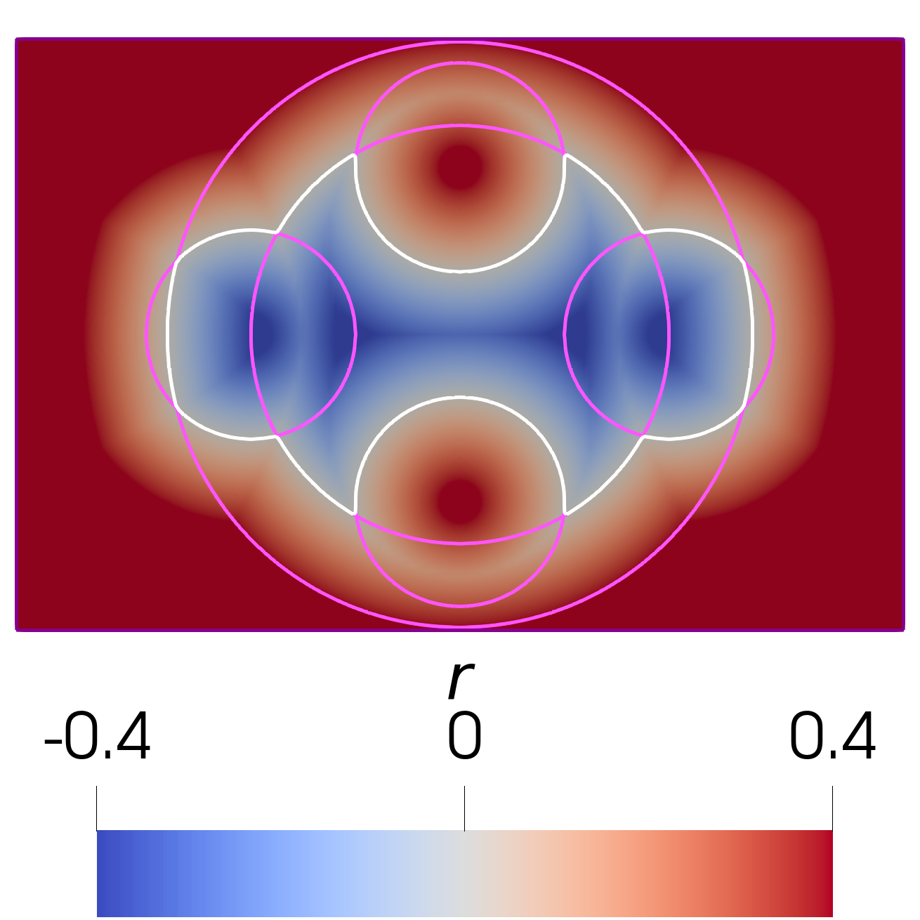
(a) omega(x)

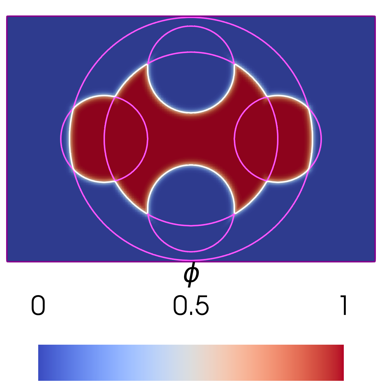
(b) omega.phi(x)

Figure 1: Constructed SDF omega in Listings 4

Note, each SDF has an optional name attribute, this can be defined during construction or assigned later. We will see in Section 4, this can be used to define boundary conditions by associating the boundary name with boundary segment it defines in the final SDF.

It is very important to acknowledge that the union, subtraction, and intersection operations do not produce a perfect SDF. This can be seen in Figure 2; this is a 1D example of two intersecting intervals. It is clear that the SDF for intersecting region does not match the true SDF.

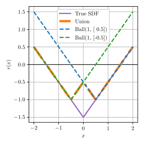
Figure 2: Errors in union of SDFs

The process of applying the Diffuse Domain method requires the SDF for two purposes. Firstly, we use it to generate a phase field function, $\phi$. As $\epsilon$ is small and the width on the interfacial region is approximately $2\epsilon$, the impact of the imperfect SDF on $\phi$ is negligible and unobservable. Secondly, the SDF is used in the extension of the boundary functions and domain functions to the full computational domain $B{}$. The Diffuse Domain method does not require the extension of these functions to be defined far from the boundary; [32] states the extension needs to be at least $3\epsilon$ from the boundaries and uses $10\epsilon$ in their experiments. So there is minimal impact from the incorrect extensions.

4 Mixed Boundaries

So far we have seen how to implement different types of boundary conditions and construct the SDFs for complex domains. For general problems it is critical to be able to combine multiple different boundary conditions. We have developed an approach to combine multiple boundary terms by partitioning the extended domain into sections, restricting the boundary term to only be in the boundary neighbourhood.

We assume the boundary conditions are defined on disjoint segments $\Gamma_{i}$ such that

$$\partial\Omega{}{}=\bigcup_{i\in I}\Gamma_{i},$$ (15)

and

$$\Gamma_{i}\cap\Gamma_{j}=\emptyset\quad\forall i,j\in I:i\neq j.$$ (16)

We assume that the different boundaries can be defined, using SDFs,

$$\Gamma_{i}=\{x|r_{i}(x)=0\}\cap\{x|r_{\Omega}{}(x)=0\},$$ (17)

where the SDFs $r_{i}$ were used together with the boolean operators to compose the domain $\Omega$. It is important that the zero sets defined by the individual SDFs do not overlap, and only intersect at a finite number of points.

$$\forall i\neq j,\;|\{x|r_{i}(x)=0\}\cap\{x|r_{j}(x)=0\}|<N\in\mathbb{N}{}.$$ (18)

Given the problem (1) with boundary conditions

$$u =g_{i} \Gamma_{i} \forall i\in I_{V},$$ on (19a)

$$(bu-D\nabla u)\cdot n =g_{c,i}-g_{v,i} \Gamma_{i} \forall i\in I_{F},$$ on (19b)

where the index sets $I_{V}$ and $I_{F}$ partition $I$ in the Dirichlet and flux boundary segments. We need to combine the additional boundary modifications terms from equations (12) and (14) to define a term ${BC}$ combining all boundary conditions.

Based on (12) and (14) the boundary conditions lead to the forcing terms in the Diffuse Domain method

$${BC}_{i} =\frac{1}{\epsilon^{3}}(1-\phi)(u-\overline{g_{i}}) \forall i\in I_{V},$$ (20a)

$${BC}_{i} =(\overline{g_{c,i}}-\overline{g_{v,i}})|\nabla\phi| \forall i\in I_{F}.$$ (20b)

To restrict these terms to specific regions combine these terms using a weighted sum

$${BC}=\sum_{i\in I_{V}\cup I_{F}}\omega_{i}{BC}_{i}.$$ (21)

In the following we discuss a possible approach to define the weights $\omega_{i}$.

Recall we provide a SDF that represents the bulk domain $\Omega{}$, $r_{\Omega}{}$. We can therefore define the mapping

$$P_{\Omega}{}(x):B{}\to\partial\Omega{}{},$$ (22)

which maps each point to its closest point on the boundary. Using the extension formula in equation (6),

$$P_{\Omega}{}(x):x\mapsto x-r_{\Omega}{}(\nabla{r_{\Omega}{}}).$$ (23)

Recall that for the flux boundaries we used the fact that the surface delta function for $\partial\Omega{}{}$ can be approximated by $|\nabla\phi|$, which is proportional to $\phi(1-\phi)$. Therefore, for boundary $\Gamma_{i}$, we use the weighting $w_{i}=4\phi_{i}(1-\phi_{i})$ to determine the location of the boundary. To obtain a domain wide weighting which restricts the boundary term, we project $w_{i}(x)$ to the point $P(x)$. Consequently,

$$w_{i,\Omega{}}(x)=w_{i}(P_{\Omega}{}(x))\approx\begin{cases}1&\text{if }x\text{ closest to }\Gamma_{i},\\ 0&\text{if }x\text{ closest to }\Gamma_{j},j\neq i.\end{cases}$$ (24)

From equation (18) the zero sets of the SDFs do not overlap, so almost everywhere we will have

$$w_{i,\Omega{}}(x)=1,w_{k,\Omega{}}(x)=0\quad\forall k\neq i.$$ (25)

This is a desired property as the solution in the neighbourhood of each boundary should only be impacted by its associated boundary condition.

However, near the intersecting points of different SDFs (as well as regions from any imperfect boolean operations), the Diffuse Domain approach results in the summation of multiple extensions of different boundary conditions. This can cause a significant error. We normalise the weights by setting

$$\omega_{i}=\frac{w_{i,\Omega{}}}{\sum_{k}w_{k,\Omega{}}}.$$ (26)

Therefore, we have $\sum_{i}\omega_{i}=1$, and average the ${BC}_{i}$ terms near these artefact points.

Using the four binary operations in ddfem.geometry to combine two SDFs, we can easily plot the different weightings. In these examples we will use two balls:

⬇

c0 = gm.Ball(radius=1, center=(0.5, 0), name="Ball0"),

c1 = gm.Ball(radius=1, center=(-0.5, 0), name="Ball1")

The union, c0 | c1, is shown in Figure 3. The right figure shows the boundary condition weighting, $\omega_{0}$, corresponding to the right Ball "Ball0". It is clear the different regions are split correctly around each Ball, however there are some artefacts around the intersection of SDFs.

(a) $\phi$

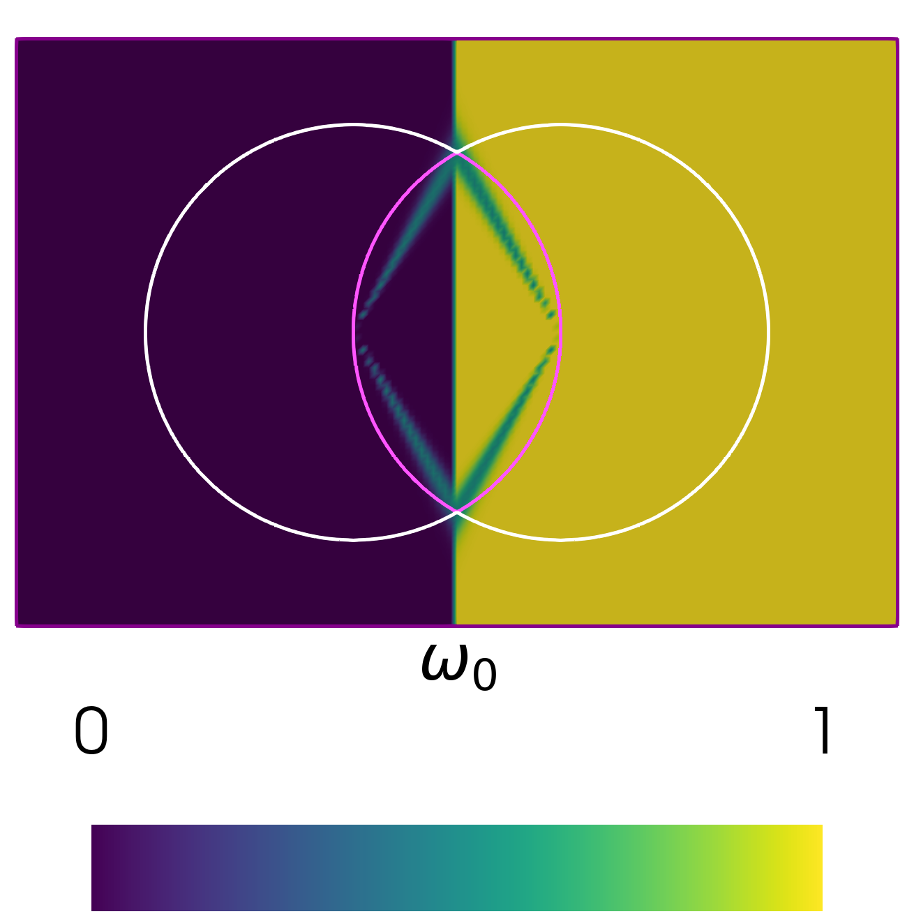
(b) $\omega_{0}$

Figure 3: Union of two Ball SDFs

Similarly, the intersection, c0 & c1, is shown in Figure 4. However, the weighting artefacts appear in the extended domain instead.

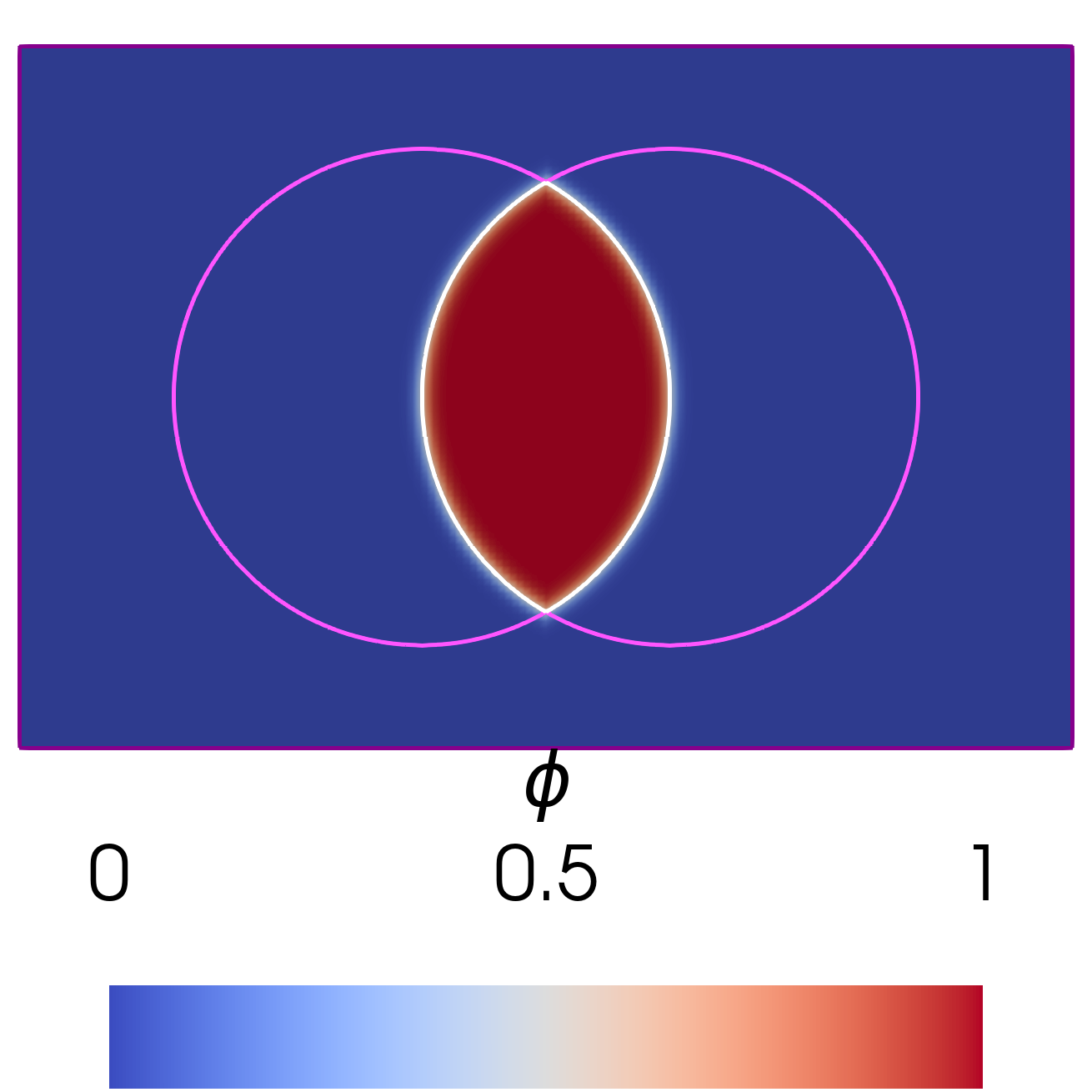
(a) $\phi$

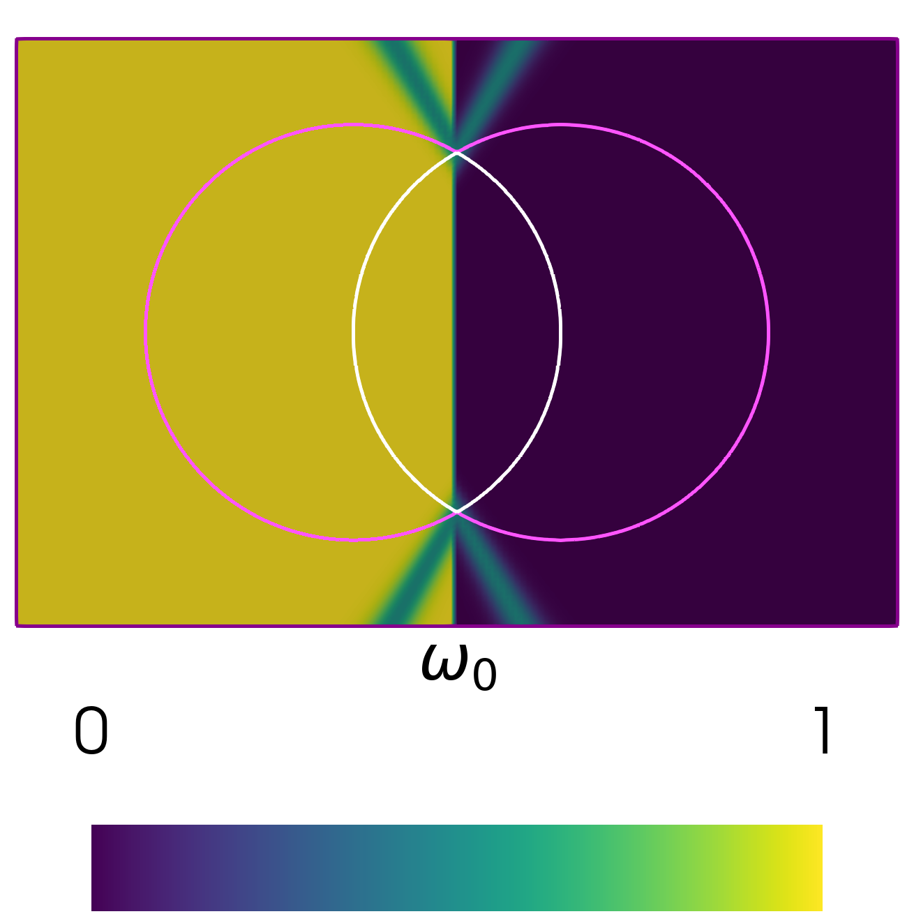
(b) $\omega_{0}$

Figure 4: Intersection of two Ball SDFs

The difference, c0 - c1, is shown in Figure 5, which has artefacts both within the extended domain.

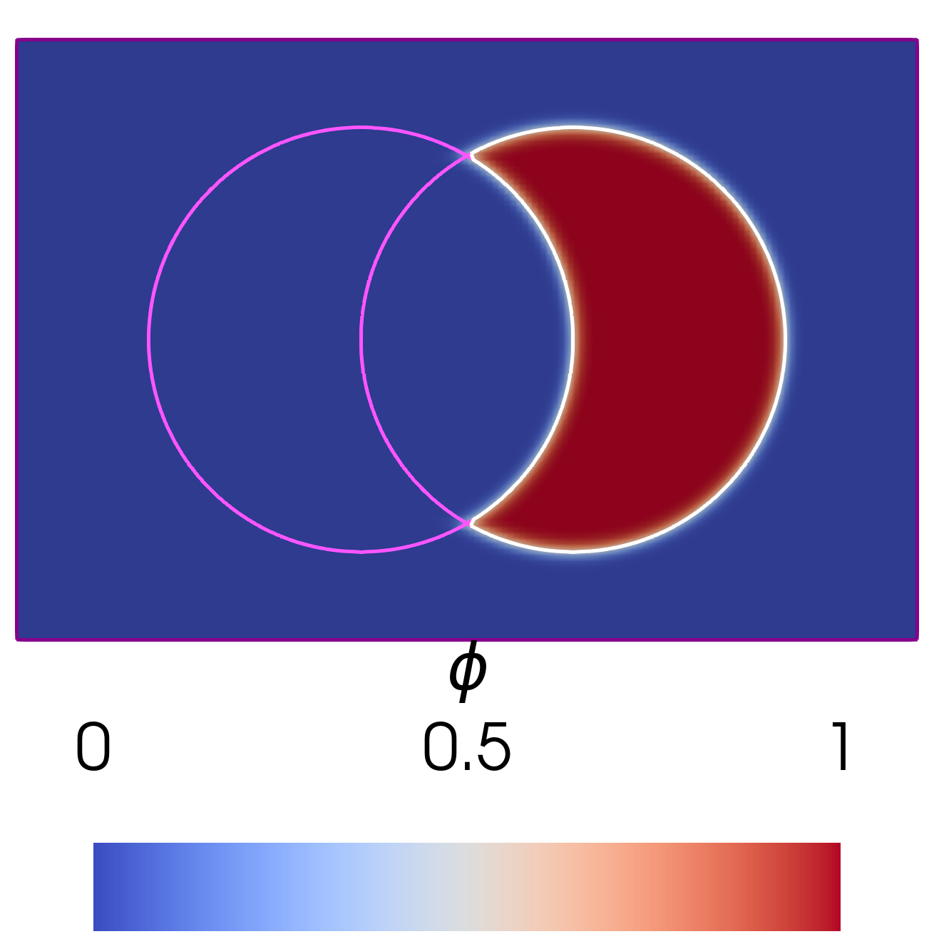
(a) $\phi$

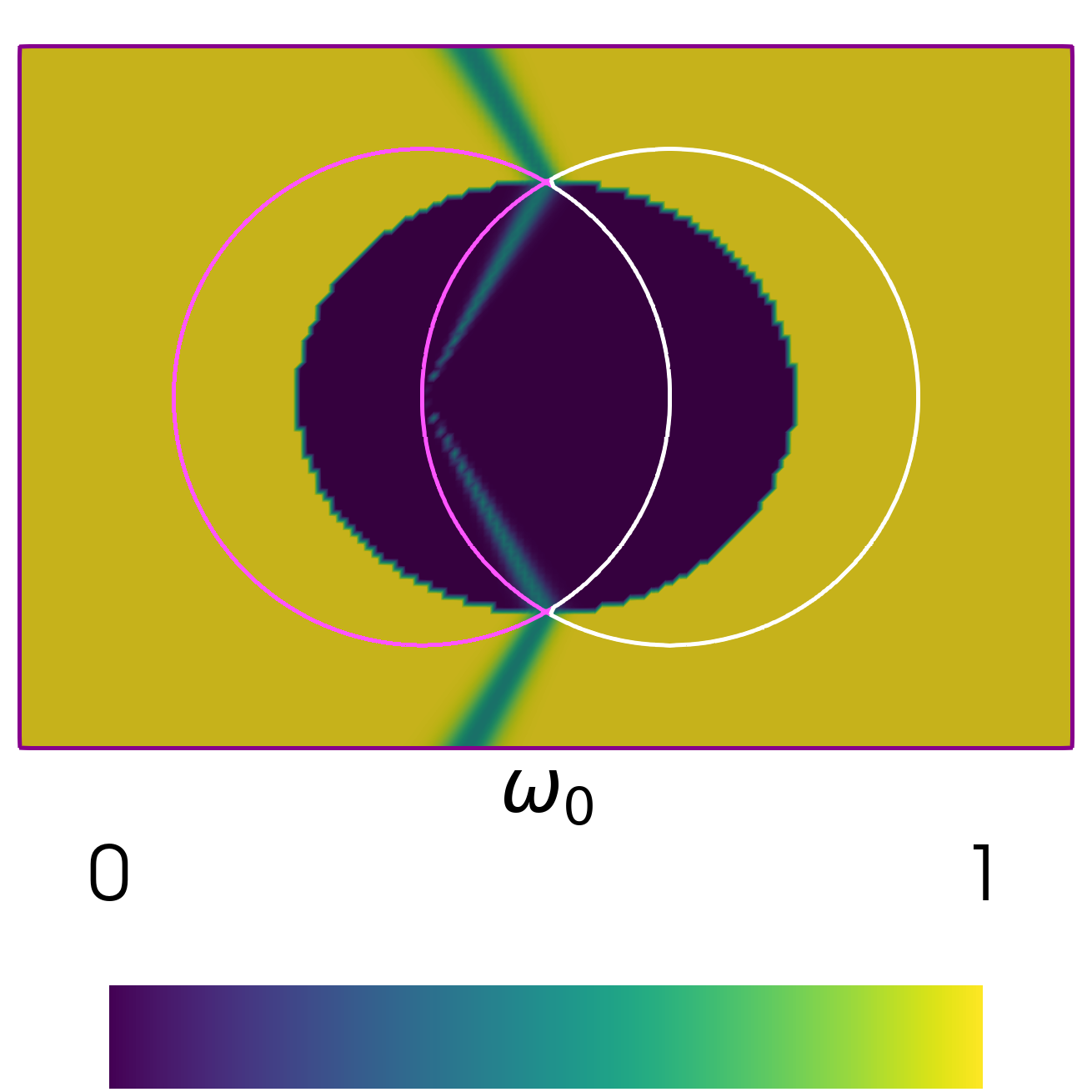
(b) $\omega_{0}$

Figure 5: Difference of two Ball SDFs

The xor, c0 ^ c1, is shown in Figure 6. As this operation creates a perfect SDF, we can see there are no stripes of artefacts similar to other operators.

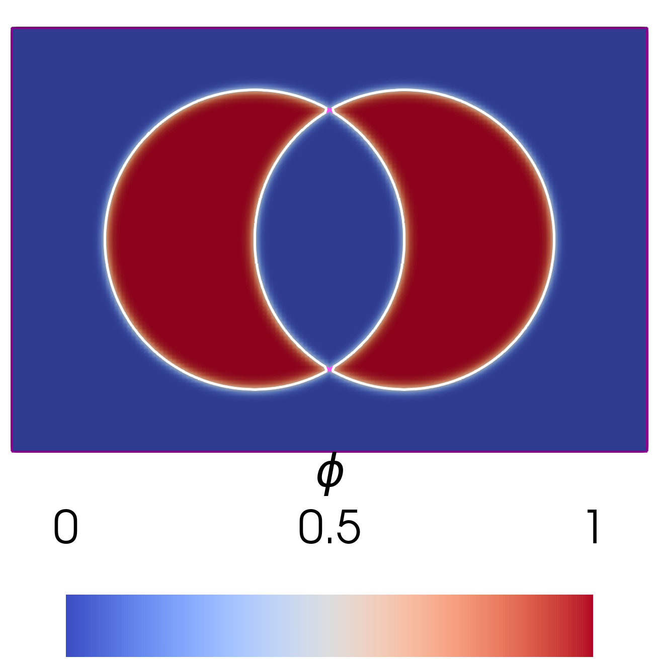
(a) $\phi$

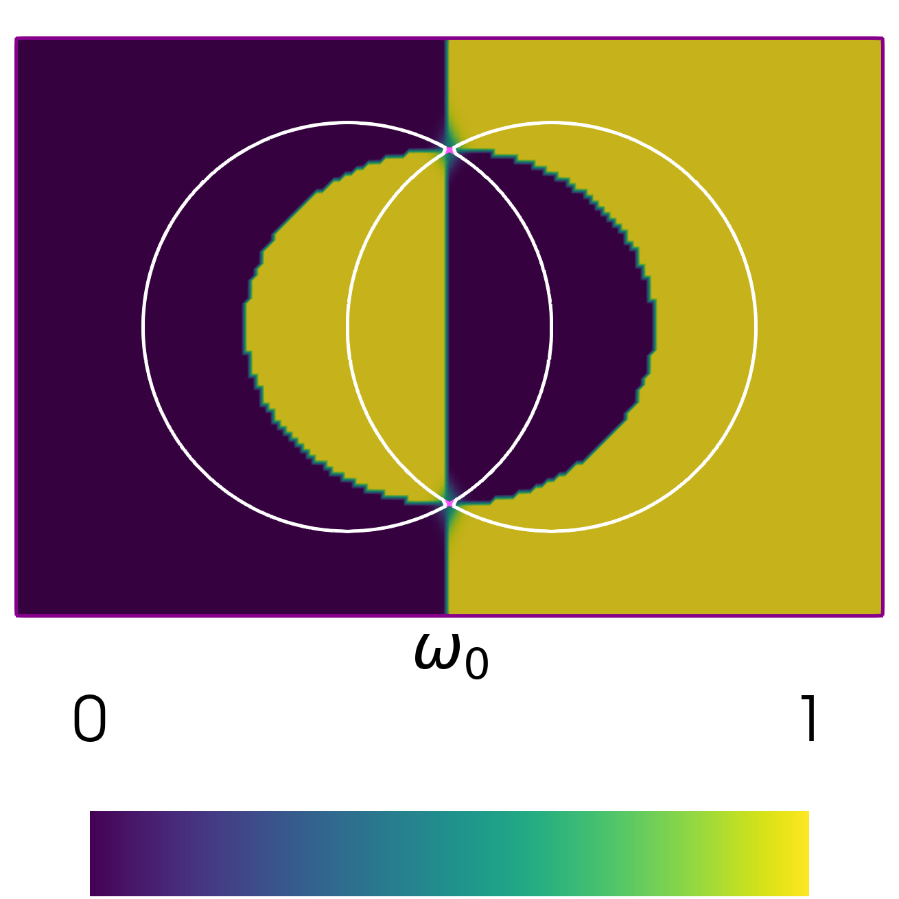
(b) $\omega_{0}$

Figure 6: Xor of two ball SDFs

Recall, $g_{i}$ needs to be defined in the neighbourhood of $\Gamma_{i}$ for the additional terms (20), so we also extended the boundary values in equations (19) using the same projection:

$$\overline{g_{i}}(x)=g_{i}(P_{\Omega}{}(x)).$$ (27)

In summary, we provide the following functions for the different boundary types

$$G_{V} =\sum_{i\in I_{V}}\omega_{i}\overline{g_{i}},$$ (28)

$$G_{F_{v}} =\sum_{i\in I_{F}}\omega_{i}\overline{g_{v,i}}|\nabla\phi|,$$ (29)

$$G_{F_{c}} =\sum_{i\in I_{F}}\omega_{i}\overline{g_{c,i}}|\nabla\phi|.$$ (30)

These boundary equations are collected into the ddfem.boundary.BoundaryTerms class. Initialised with a given Model and SDF, this class provides an easy way to implement the boundary conditions in a Diffuse Domain model. It also extends the boundary data to be compatible with the Diffuse Domain approximation. It provides the key methods:

• BndValueExt: returns $G_{V}$, or None if no Dirichlet boundaries,

• jumpV: returns a weighted sum with $u$, $\sum_{i\in I_{V}}\omega_{i}(u-\overline{g_{i}})$,

• BndFlux_vExt, returns $G_{F_{v}}$, or None if no flux boundaries.

• jumpFv, returns a weighted sum with $F_{v}$, $\sum_{i\in I_{V}}\omega_{i}(F_{v}n-\overline{g_{v,i}})\delta_{\partial\Omega{}{}}$,

• BndFlux_cExt: returns $G_{F_{c}}$.

The Model.boundary attribute is a dictionary, and its keys determine how the boundary conditions are handled. A key is assumed to be a boundary condition for the diffuse interface when it is either an instance of the SDF class, or the string matching the SDF.name attribute of the associated instance. Other keys are assumed to be boundary conditions for the computational mesh and will be left unchanged by the Diffuse Domain transformer functions. The corresponding value in the dictionary is the boundary function e.g., $g$, $g_{c}$, $g_{v}$. For example, using the SDF from Figure 1 we can set the boundary conditions:

⬇

Model.boundary = {

bulk: [

BndFlux_c(g_c),

BndFlux_v(g_v),

],

"Cutoff": BndValue(g),

}

Note, the implementations requires using the dictionary value to be one of the following classes:

• BndValue

• BndFlux_c

• BndFlux_v

• [BndFlux_c, BndFlux_v]

The required boundary flux (BndFlux_c, BndFlux_v, or the list of both) corresponds to whether the source terms $F_{c}$ and $F_{v}$ are defined in the problem. This wrapper allows easy identification of the different boundary types. We finally provide the function ddfem.model2ufl which takes a model class and its boundary dictionary, converting it to a full UFL form.

Using the above we arrive at the following updated model for the DDM1 approach:

Listing 5: Model of DDM1 approximation.

⬇

class ModelDDM1:

BT = BoundaryTerms(Model, omega)

boundary = BT.physical

bp = BT.domain.boundary_projection

ep = BT.domain.xternal_projection

def S_e(t, x, U, DU):

return BT.BndFlux_cExt(x, U)

def S_i(t, x, U, DU):

source = phi(x) * (f(ep(x)) - c(ep(x)) * U)

bc_v = -BT.jumpV(x, U) * (1 - phi(x)) / (epsilon**3)

bc_fv = BT.BndFlux_vExt(x, U, DU)

return source + bc_v + bc_fv

def F_c(t, x, U):

return phi(x) * outer(U, b(ep(x)))

def F_v(t, x, U, DU):

return phi(x) * D(ep(x)) * DU

Then the completed UFL form is obtained using:

⬇

ufl_form = model2ufl(ModelDDM1, space)

The ddfem.geometry.Domain class collects the functions related to the boundaries. This acts similar to the SDF class for the $r_{\Omega}{}$, initialising with Domain(omega). The key methods implemented for the modification of the integrals are:

• phi: $\phi(x)$,

• scaled_normal: $-\nabla(\phi(x))$,

• surface_delta: $|\nabla(\phi(x))|$,

• normal: $-\nabla(\phi(x))/|\nabla(\phi(x))|$

• bndProjSDFs(SDFname): maps from the SDF $r_{i}$ to the unnormalised weight $w_{i}(x)$ (24), using its attribute SDF.name.

An instance of this class is automatically constructed in the class BoundaryTerms if a SDF is given. However, it can be initialised and modified by the user beforehand for advanced applications.

5 Transformers

Our main goal is to simplify implementing and using different Diffuse Domain approaches, so we now introduce the transformers subpackage. This implements a group of new functions to transform an existing Model (Listing 2) and a SDF class, returning a new model class defined in domain $B{}$ based on a wide range of Diffuse Domain methods.

First, any transformer should call the function pretransformer to return a new model class. This will construct the BoundaryTerms class, to set up the extended boundaries and additional boundary terms. To improve performance, we have found it beneficial to include the extra default boundary condition:

⬇

boundary[lambda x: domain.omega.chi(x) < 0.5] = BndValue(BT.BndValueExt)

On any boundaries in the extended domain, $\partial B{}{}\backslash\partial\Omega{}{}$, we use the extended value of the Dirichlet boundary conditions. However, if only flux boundary conditions are given, we use the extended value of the flux boundary conditions:

⬇

valFc = BndFlux_c(lambda t, x, U, n: -BT.BndFlux_cExt(t, x, U))

valFv = BndFlux_v(lambda t, x, U, DU, n: BT.BndFlux_vExt(t, x, U, DU))

boundary[lambda x: domain.omega.chi(x) < 0.5] = [valFc, valFv]

A further important role of ddfem.transformers.pretransformer is to extend all the term and coefficient functions. This redefines all methods (e.g., S_i, F_v) using external_projection to simplify implementing transformers.

A transformer class, DDModel, is implemented using a similar structure to Listing 5. In Section 4, we saw that while the viscous $F_{v}$ and convective $F_{c}$ flux terms are simply multiplied by $\phi$, the source terms are augmented by new boundary and potential stability terms. This requires implementing separate methods to split the different components of the source terms. Finally, calling the ddfem.transformers.posttransformer function with DDModel constructs only the required methods to be compatible with the Listings 1 and ensures only existing methods are available in the new model. The effects of posttransformer on different methods are shown in Table 1.

DDModel Method	Methods Included	Model requirement
DDModel.S_e	S_e_source	S_e
	S_e_convection	F_c
	S_outside	outFactor_e
DDModel.S_i	S_i_source	S_i
	S_i_diffusion	F_v
	S_outside	outFactor_i
DDModel.F_c	F_c	F_c
DDModel.F_v	F_v	F_v

Table 1: Composition of methods in the transformed DDModel class

Note, the attributes outFactor_e and outFactor_i are used as scaling factors for S_outside. At least one is required to if Dirichlet boundary conditions are used.

The decorator ddfem.transformers.transformer is implemented to simplify the use of pretransformer and posttransformer. A complete implementation of the DDM1 transformer is given below:

⬇

@ddfem.transformers.transformer

def DDM1(Model):

class DDModel(Model):

def S_e_source(t, x, U, DU):

return DDModel.phi(x) * Model.S_e(t, x, U, DU)

def S_e_convection(t, x, U, DU):

return -DDModel.BT.BndFlux_cExt(t, x, U)

def S_outside(t, x, U, DU):

return -(

DDModel.BT.jumpV(t, x, U) * (1 - DDModel.phi(x)) / (DDModel.epsilon**3)

)

def S_i_source(t, x, U, DU):

return DDModel.phi(x) * Model.S_i(t, x, U, DU)

def S_i_diffusion(t, x, U, DU):

if DDModel.BT.BndFlux_vExt is not None:

diffusion = DDModel.BT.BndFlux_vExt(t, x, U, DU)

else:

diffusion = zero(U.ufl_shape)

return diffusion

def F_c(t, x, U):

return DDModel.phi(x) * Model.F_c(t, x, U)

def F_v(t, x, U, DU):

return DDModel.phi(x) * Model.F_v(t, x, U, DU)

return DDModel

Again, this model can be used with model2ufl and the returned UFL form can then be used with any solver and mesh defined on $B{}$, or further modified. Currently, the package includes the following transformers:

• DDM1

• Mix0DDM

• NDDM

• NSDDM

Furthermore, the transformers are implemented to allow time dependent coefficients. Examples of using these transformer functions will be shown in Section 6.

6 Experiments

We conclude by comparing the performance of the Diffuse Domain transformers over a range of different problems. We have already seen DDM1, but we will also make comparisons to Mix0DDM and NSDDM. The specific formulation of these methods is not the focus of this work. However, we should note that Mix0DDM was designed with a focus on Dirichlet boundary conditions and improved gradient approximation, but can display some stability issues with full flux boundaries. These methods are a part of our current research and their derivation and properties will be explored in a separate paper.

For all experiments we will use Dune-Fem[36] to compute the approximate solution. A benefit of using Dune-Fem in the Diffuse Domain context is the availability of adaptive and filtered grid view. The filtering allows us to define a simple rectangular mesh, and then remove points far away from the diffuse boundary, reducing the mesh, resulting in fewer degrees of freedom. Removing mesh elements can be easily done using the SDFs, we decided to remove all mesh elements with $r(x)>10\epsilon$. Note, due to the imperfect nature of operating on SDFs, the filtering may include unexpected regions further away than the original boundary, $\partial\Omega{}$. Using the domain in Listings 4, we get an extra loop at the top and bottom of the cut away regions, which can be seen in Figure 7.

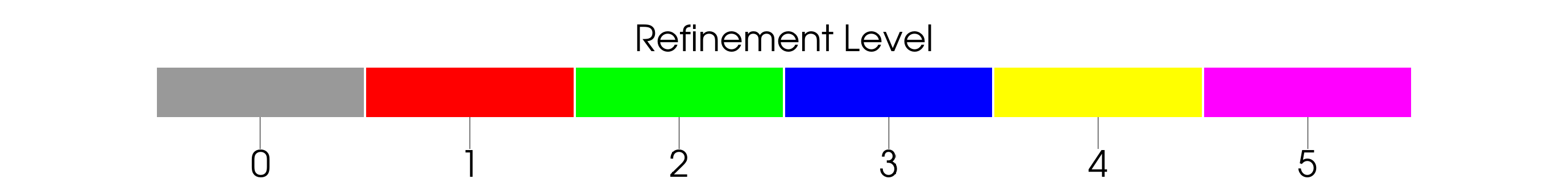
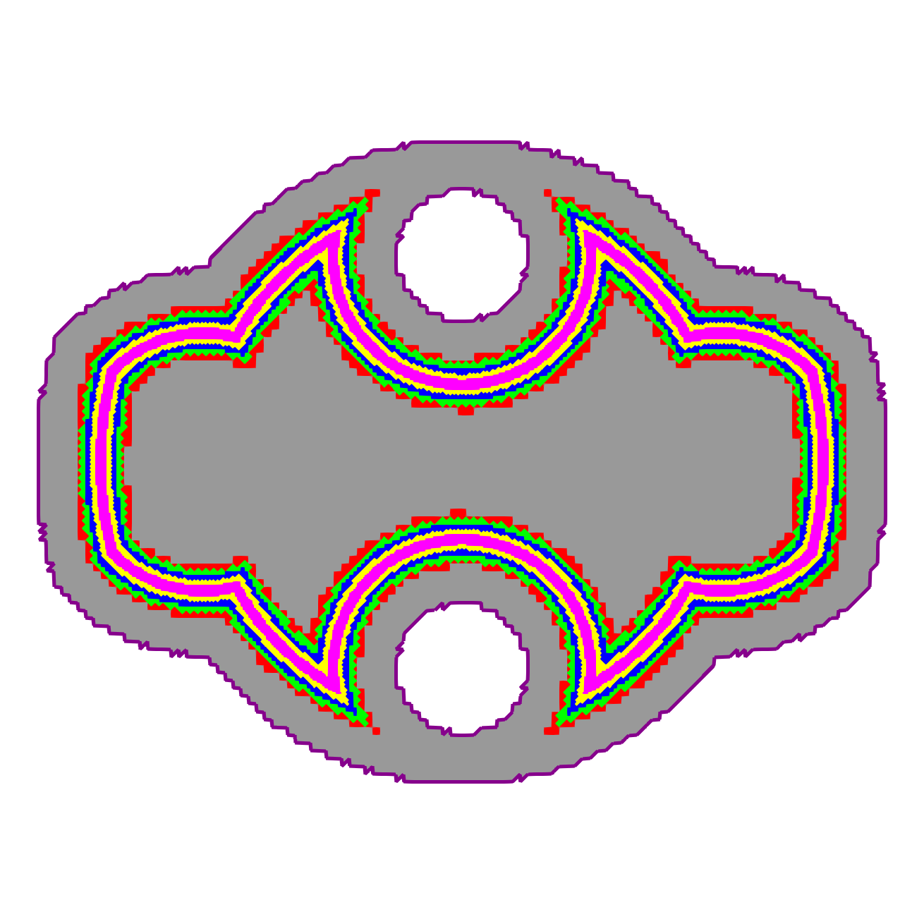
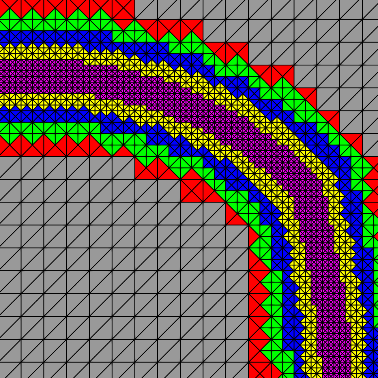
Figure 7: Adapted and filtered grid view using Dune-Fem

When used with Dune-Fem, ddfem also provides a straight forward way to locally adapt the mesh around the boundary $\partial\Omega{}$. We use the surface delta function, which we approximated using $\phi(1-\phi)$ in (24), to mark elements for refinement that are in the interfacial region. For the experiments, we use five levels of refinement across a width of $4\epsilon$. The levels of refinement for the domain from Listings 4 are show in Figure 7. This combination of adaptivity and filtering can produce a mesh with a comparable number of elements to a fitted mesh.

ddfem is available on PyPi and can be installed using pip install ddfem. Currently, ddfem relies on a pre-release version of Dune-Fem, and we recommend using pip install ddfem[dune] to install the correct version of Dune-Fem together with ddfem. More details on installation and usage can be found on GitLab page for ddfem https://gitlab.dune-project.org/dune-fem/ddfem and the tutorial available under https://ddfem.readthedocs.io/en/latest/index.html.

6.1 Poisson’s equation

First, we will look at a simple diffusion problem.

$$-\Delta\psi=-1\quad\text{ in }\Omega{},$$ (31a)

$$\psi=0\text{ on }\partial\Omega{}{},$$ (31b)

We will use the domain given by the following SDF:

Listing 6: Defining a three ball SDF

⬇

sdfs = [

Ball(radius=0.3, center=(0.15, 0.15)),

Ball(radius=0.3, center=(0.15, 0.15)),

Ball(radius=0.4, center=(0, 0))

]

omega = (sdfs[0] | sdfs[1]) & sdfs[2]

We will compare the results across a fitted mesh without using the Diffuse Domain approach, and a non-fitted mesh. Both meshes are refined around the boundary of $\Omega$ based on the value of the phase field function. The results in Figure 8 show the effectiveness of the method as they are very close to each other.

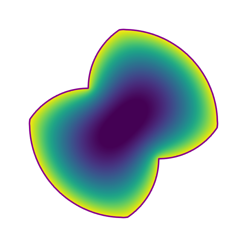
(a) Fitted

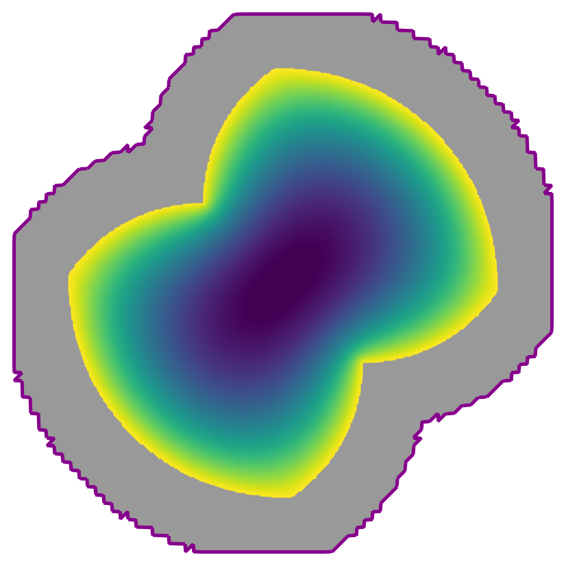
(b) DDM1

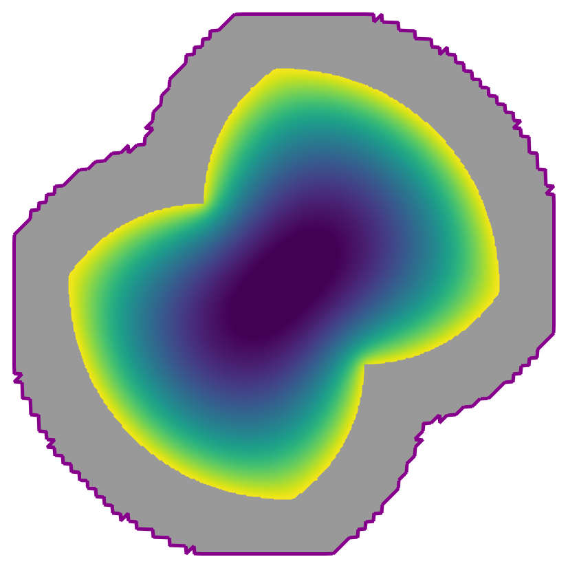
(c) Mix0DDM

Figure 8: Comparison of the approximate solution to Poisson’s equation using Diffuse Domain method to a fitted mesh

6.2 Chemical Reaction

We study a reaction-diffusion-advection problem for three species $u_{0},u_{1},u_{2}$, this problem was investigated on a square domain in [39]. The velocity field is given by $V=(\nabla\psi)^{\perp}$, where we use the discrete solution $\psi$ to the previous problem. Computing this vector field in Figure 9 show that the velocity field are closely matched away from the boundary. However, DDM1 shows a small boundary layer with low velocity, and a smaller peak velocity compared to the others. Mix0DDM has the largest region of velocity at the inner cusps, and smaller magnitude than the fitted mesh. This is expected as Mix0DDM is designed to approximate gradients more accurately. This demonstrates the importance of choosing the correct Diffuse Domain approximation for a given problem, and the benefit of ddfem collecting multiple transformers for the user.

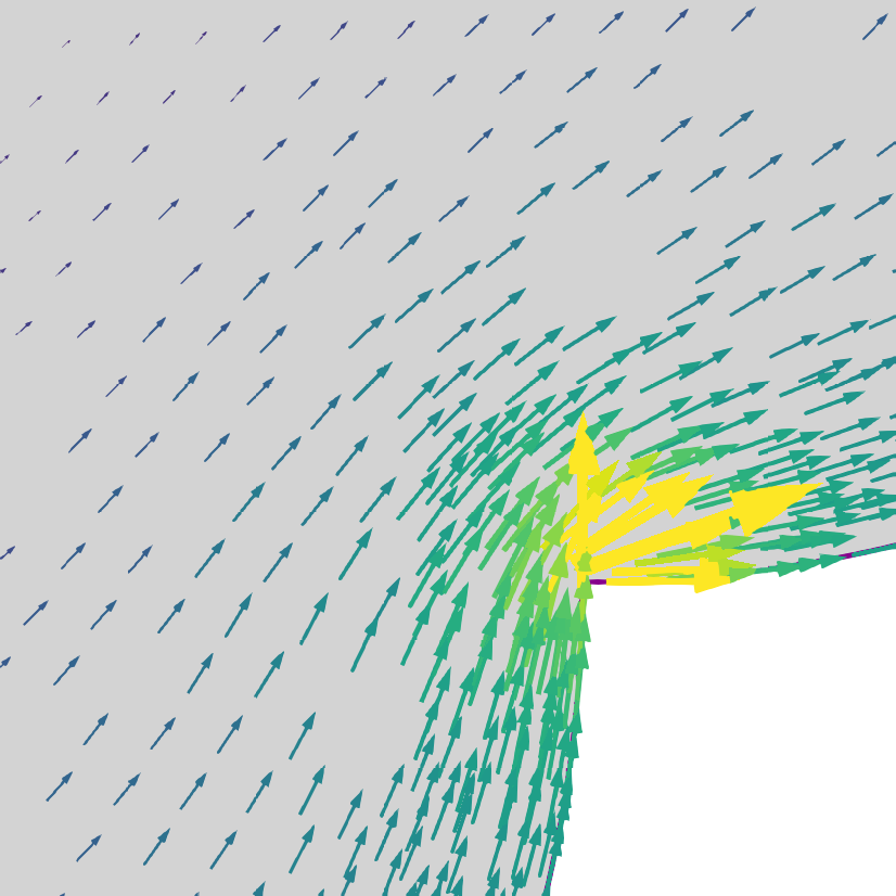
(a) Fitted

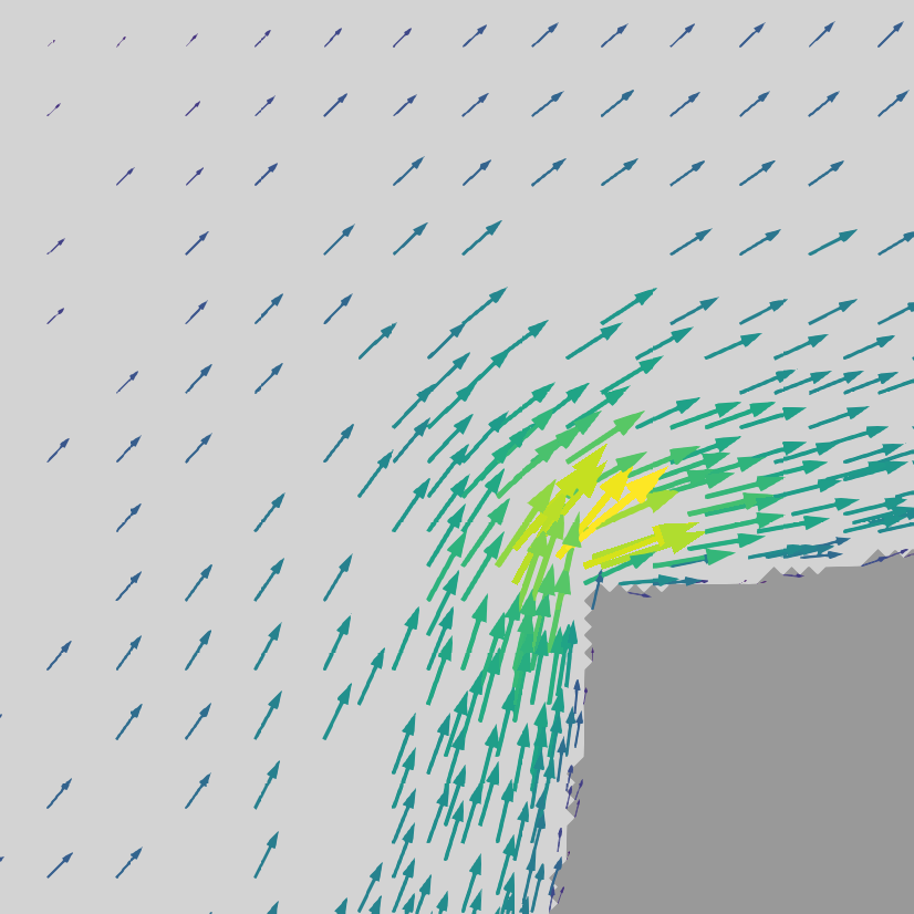
(b) DDM1

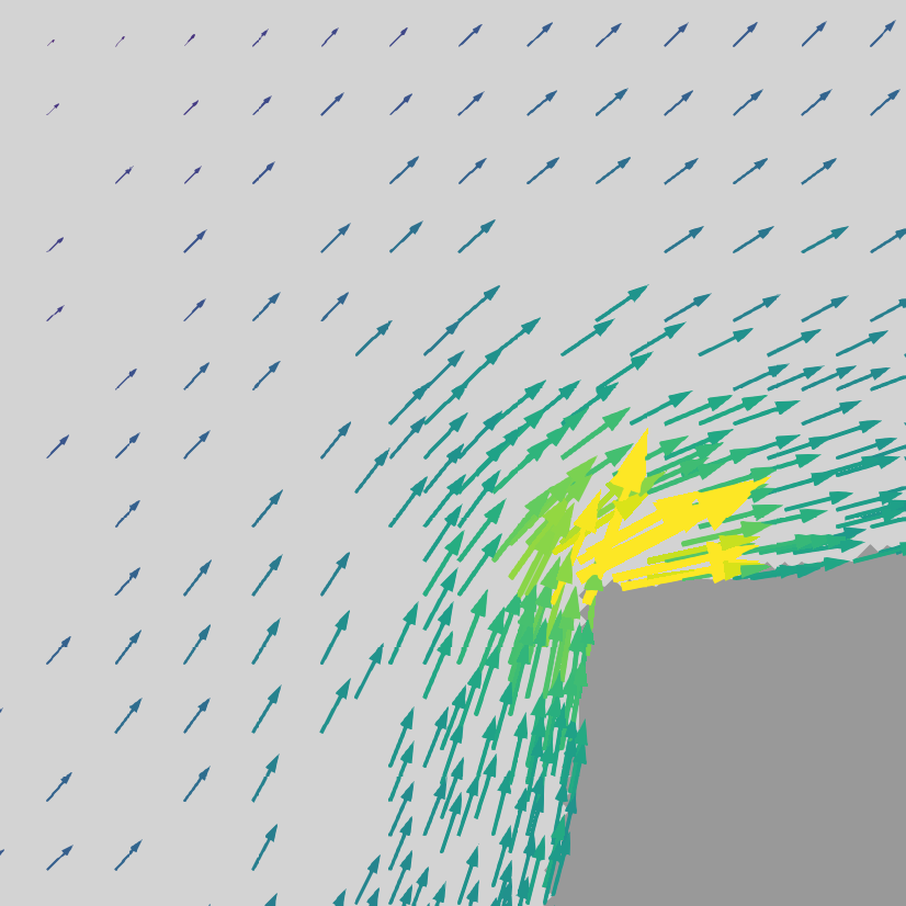
(c) Mix0DDM

Figure 9: Discrete chemical reaction velocity computed from Figure 8, zoomed on lower cusp

We create two sources at opposite points in the shape $\Omega$ close to the boundary

$$p_{1} =\left(-0.25,-0.25\right)^{T}, p_{2} =\left(0.25,0.25\right)^{T}.$$ (32)

The source term $F(t,x)$ is active for $t<10$ in circles around these points,

$$f_{i}(x) =\begin{cases}5&\text{if }\|x-p_{i}\|<0.04\\ 0&\text{otherwise}\end{cases} F(t,x) =\begin{cases}\left(f_{1}(x),f_{2}(x),0\right)^{T}&\text{if }t<10\\ \left(0,0,0\right)^{T}&\text{otherwise}\end{cases}$$ (33)

The reaction causes $u_{0}$ and $u_{1}$ to convert into $u_{2}$:

$$R(u)=\left(u_{0}u_{1},u_{0}u_{1},-2u_{0}u_{1}\right)^{T}.$$ (34)

Combining these components gives the following problem, with diffusion $D=0.001$, a reaction rate $k=10$, and using a semi-implicit scheme with time step $dt=0.05$:

$$\frac{u^{n}-u^{n-1}}{dt}+\nabla\cdot(u^{n}\otimes V-D\nabla u^{n})=F(t,x)-kR(u^{n-1})\quad\text{ in }\Omega{},$$ (35a)

$$(D\nabla u^{n}-u^{n}\otimes V)n=0\text{ on }\partial\Omega{}{},$$ (35b)

$$u^{0}=(0,0,0).$$ (35c)

Looking at the results at early times in the simulation in Figure 10, we can see very similar results of the chemicals transporting around the boundary, and a small diffusion towards the centre.

	Fitted	DDM1	Mix0DDM
$n=120$
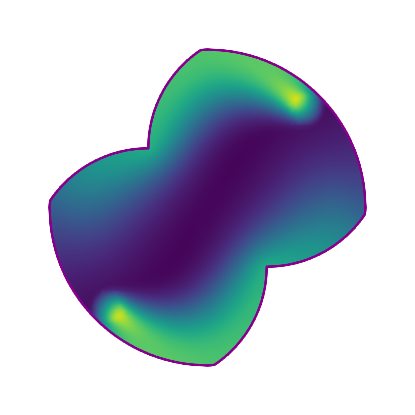
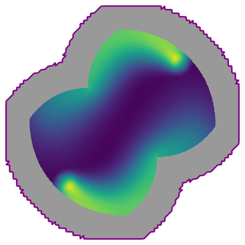
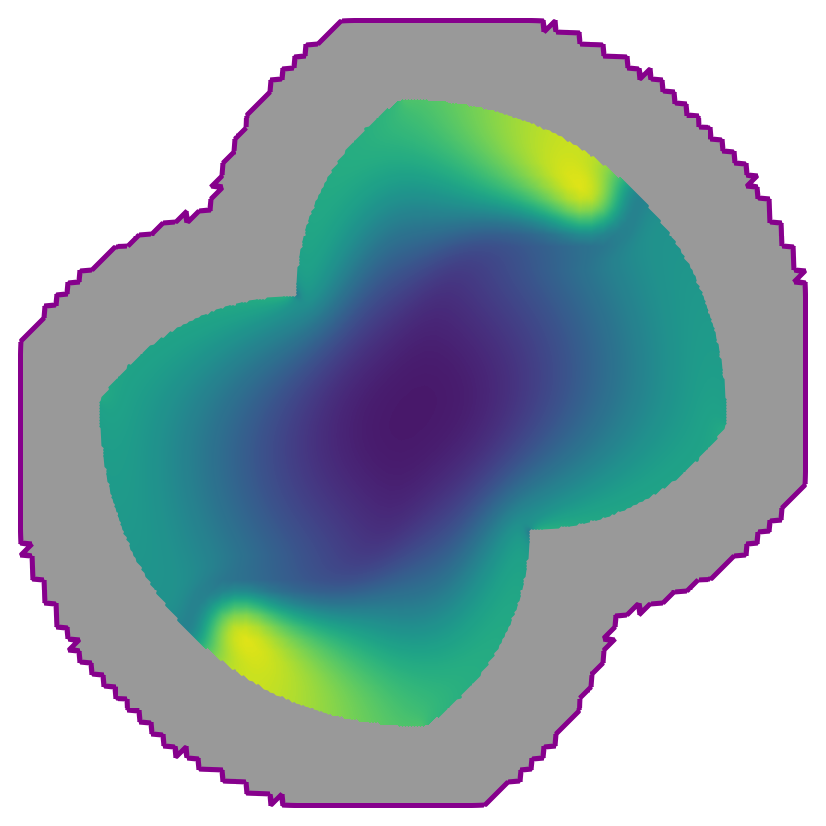
$n=200$

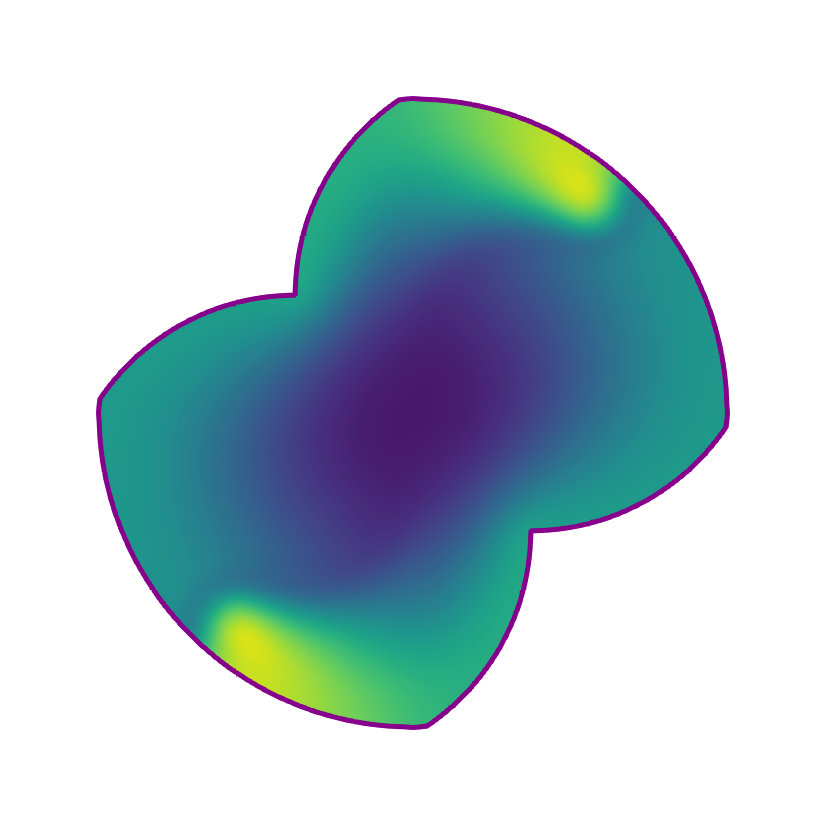
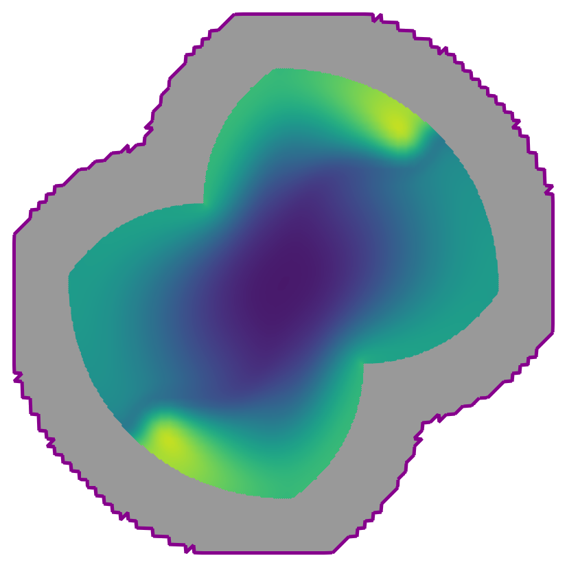
Figure 10: Approximate solution to chemical reaction problem until source inactive

However, at later times shown in Figure 11 (note the different scale), it is clear that the transportation in DDM1 is behind the fitted solution and Mix0DDM. This happens due to the lower velocity observed in Figure 9. Also, Mix0DDM appears to maintain a higher chemical concentration throughout.

	Fitted	DDM1	Mix0DDM
$n=320$
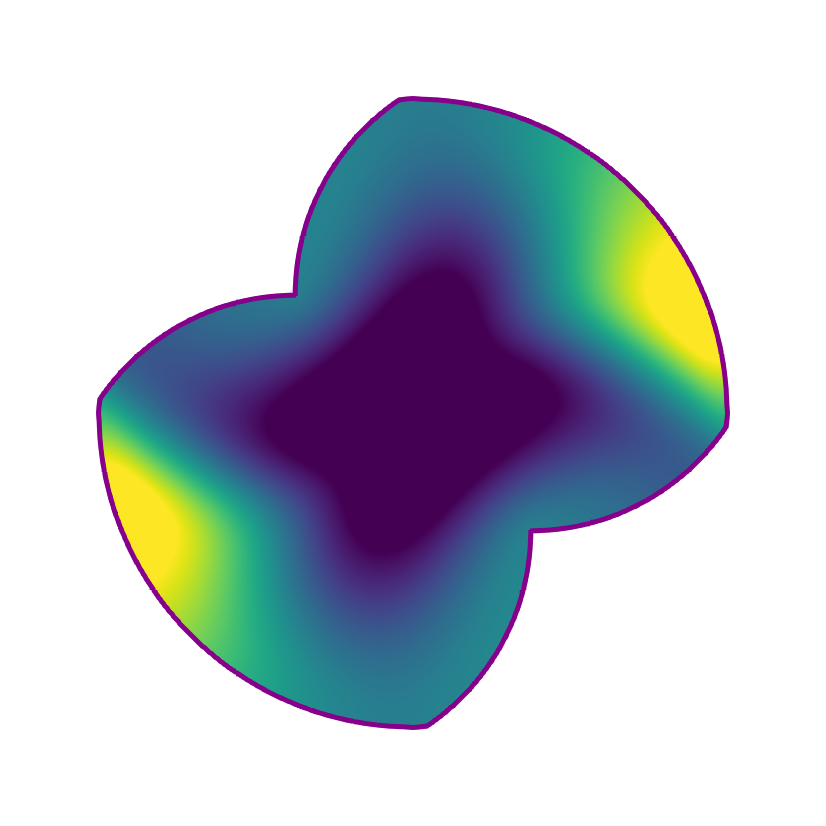
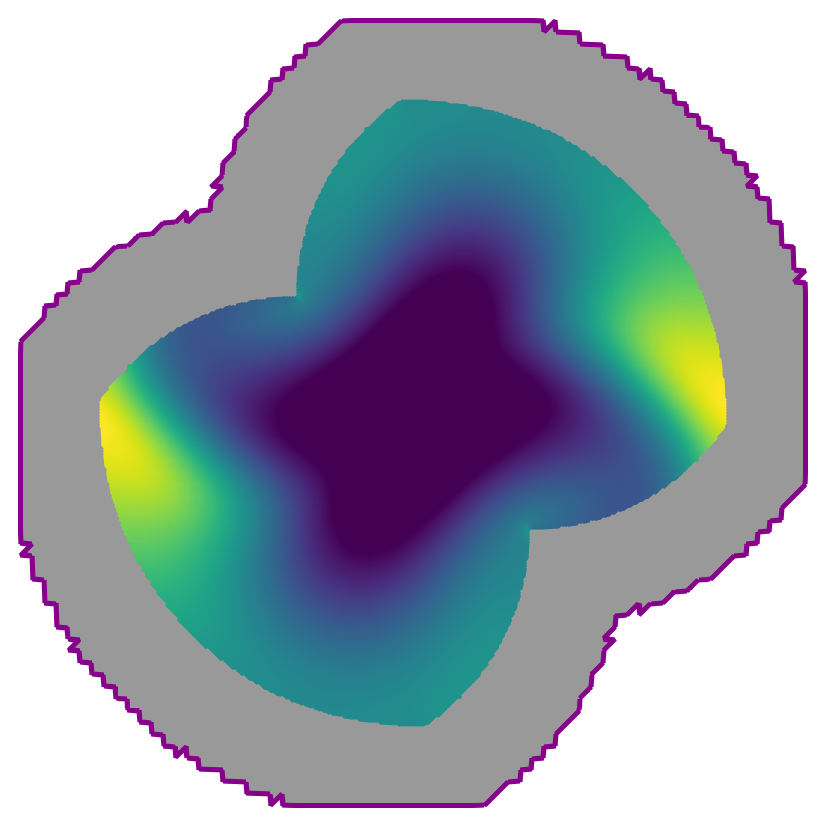
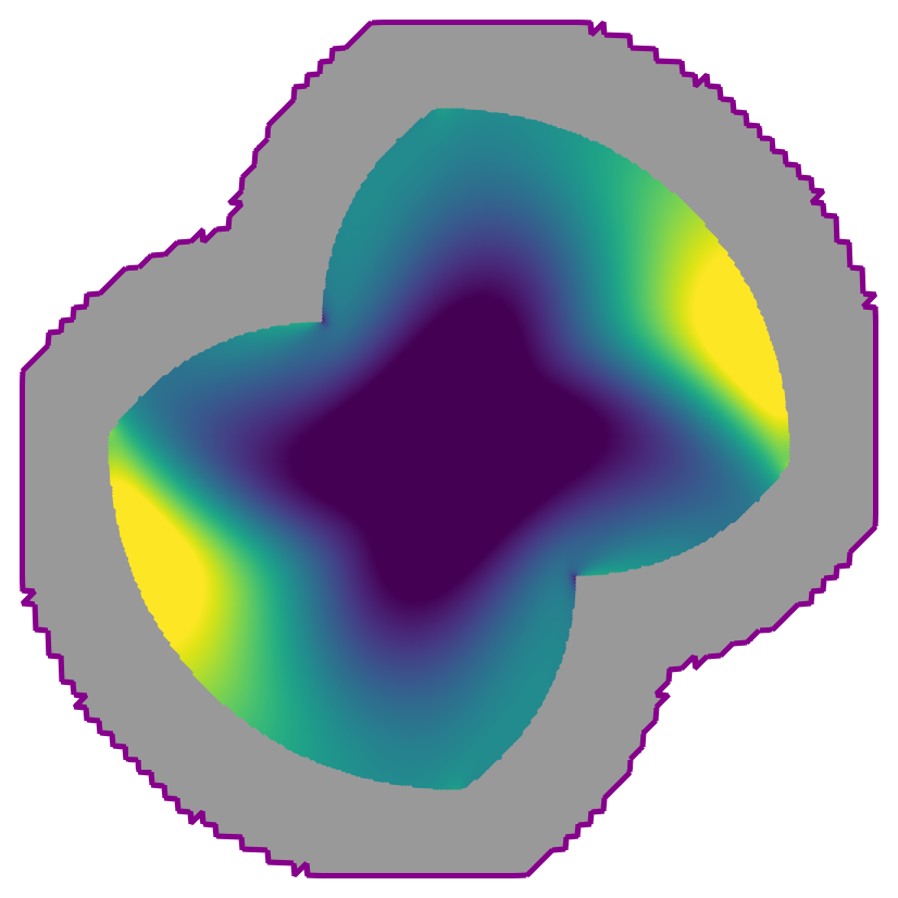
$n=520$

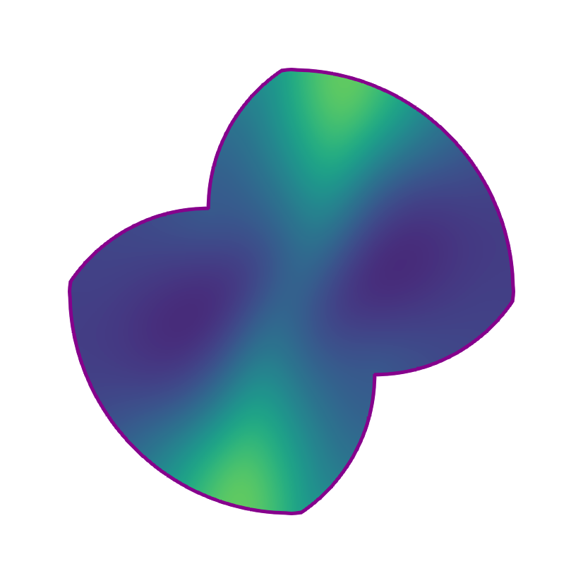
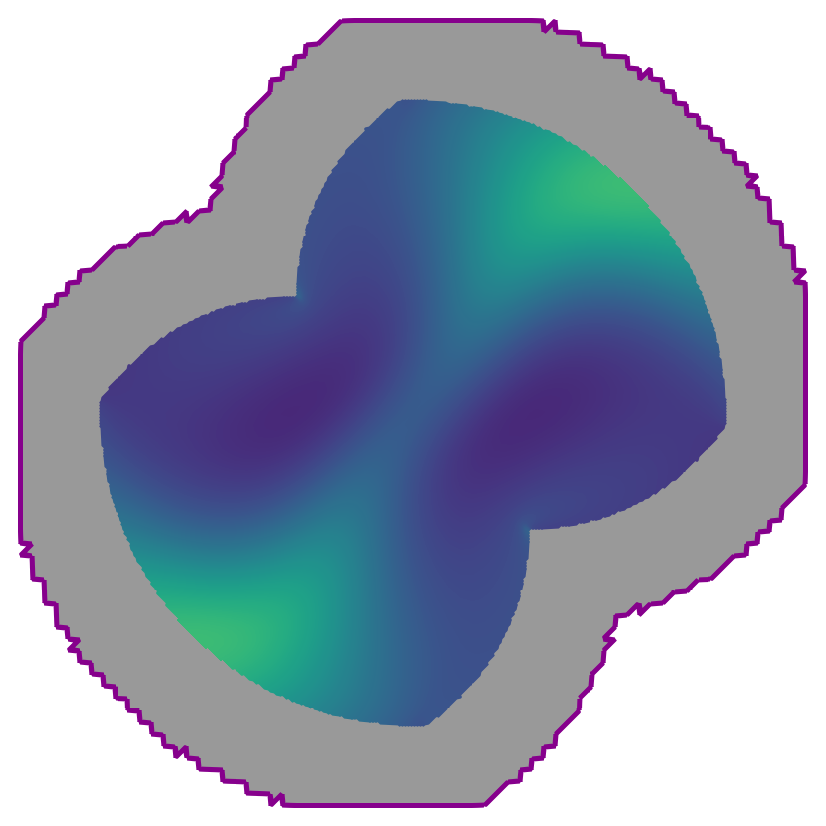
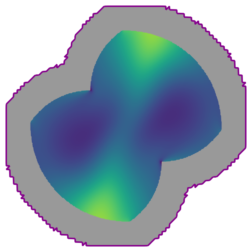
Figure 11: Approximate solution to chemical reaction problem after source inactive

6.3 Cahn-Hilliard equation

The Cahn-Hilliard equation has been explored with the Diffuse Domain method before [26]. We will solve the Cahn-Hilliard equation by splitting the fourth order equation into a system of second order equations, the concentration field $c$ and the chemical potential $\mu$. Using the Crank-Nicolson method with time step $dt=5\times 10^{-6}$ until 0.001 and $dt=4\times 10^{-5}$ until 0.008 we get,

$$\frac{c^{n}-c^{n-1}}{dt}-0.5\Delta(\mu^{n}+\mu^{n-1})=0\quad\text{ in }\Omega{},$$ (36a)

$$\mu^{n}-\frac{df(c^{n})}{dc}+\lambda\Delta c^{n}=0\quad\text{ in }\Omega{}.$$ (36b)

This uses the double well potential, $f(c)=100c^{2}(1-c)^{2}$, with $\frac{df(c)}{dc}=200c(2c^{2}-3c+1)$ and gradient energy $\lambda=0.01$.

The ddfem package can transform systems of equations. However, there is currently a limitation that they will have the same type of boundary condition if defined by the same model class. So we have the boundary conditions,

$$\nabla\mu^{n}n =0\text{ on }\partial\Omega{}{}, \lambda\nabla c^{n}n =0\text{ on }\partial\Omega{}{}.$$ (37)

Note due to the stability issues with Mix0DDM, we will show results using NSDDM.

We initialise the concentration with a small oscillating region in the centre of the domain:.

$$c^{0}(x) =\begin{cases}0.5+0.1\sin(20\pi x_{1})\sin(20\pi x_{2})&\text{if }|x_{1}|,|x_{2}|<0.1\\ 0.5&\text{otherwise}\end{cases} \mu^{0} =\mu^{0}=\frac{df(c^{0})}{dc}-\lambda\Delta c^{0}.$$ (38)

We take the domain from the previous example with the SDF given in Listings 6. However, due to influence of the mesh on the projection of the initial conditions and the resulting changes to the solution, we chose to use meshes that match on the original $\Omega{}$ for both the fitted and the unfitted simulations. So a different mesh is used from the previous example, we used Gmsh to produce a conforming mesh with identical interiors. This gives the results in Figure 12.

	Fitted	DDM1	NSDDM
$n=5$
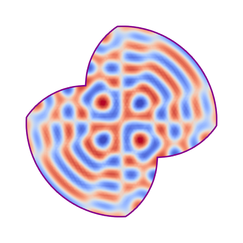
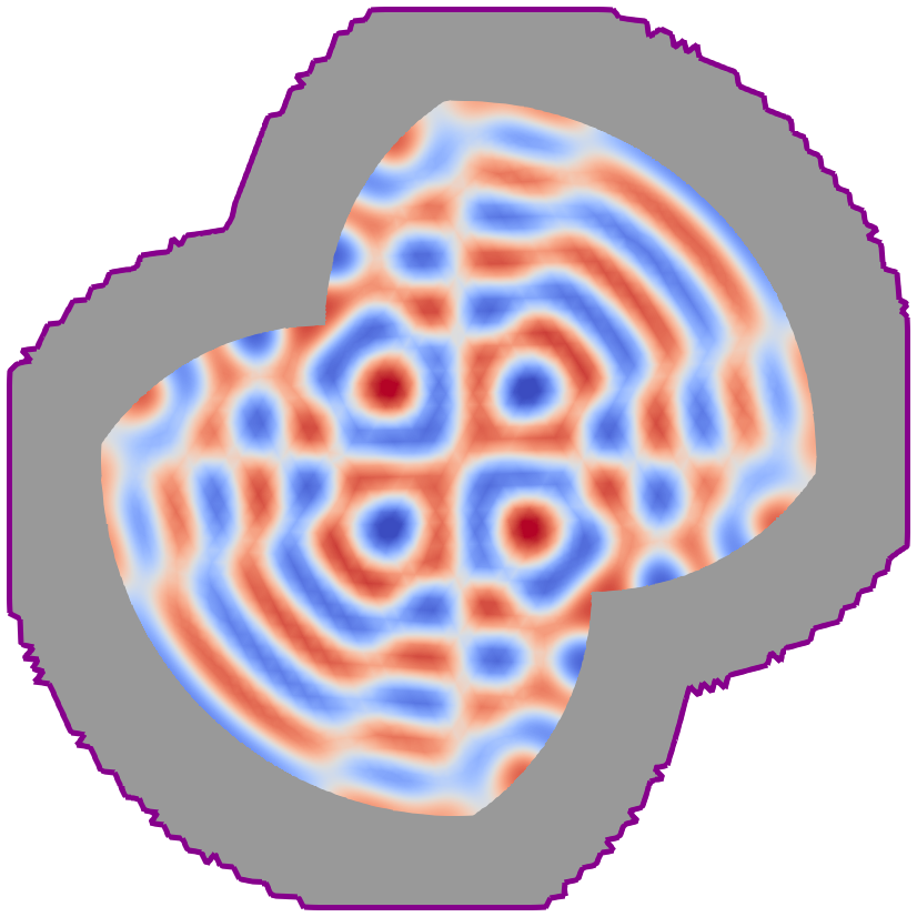
$n=20$
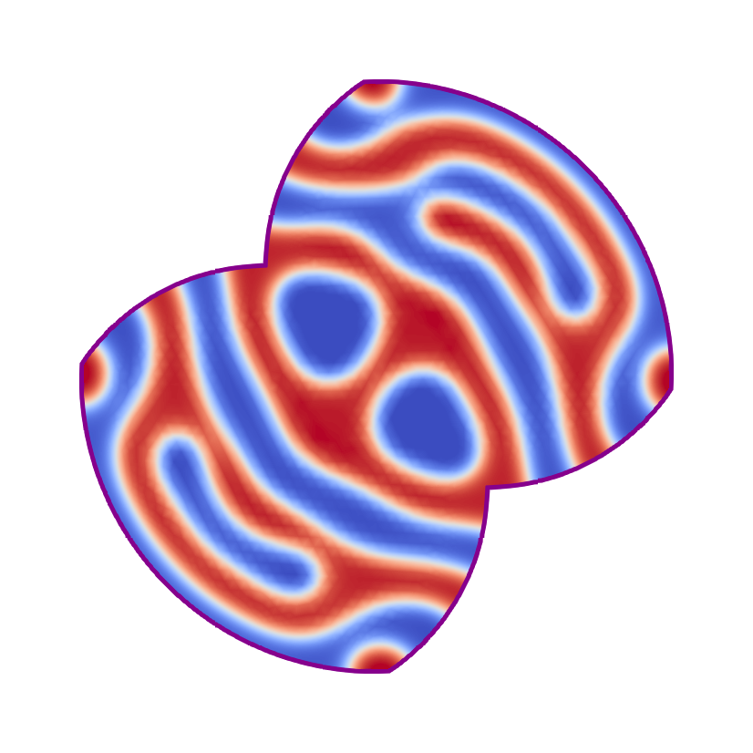
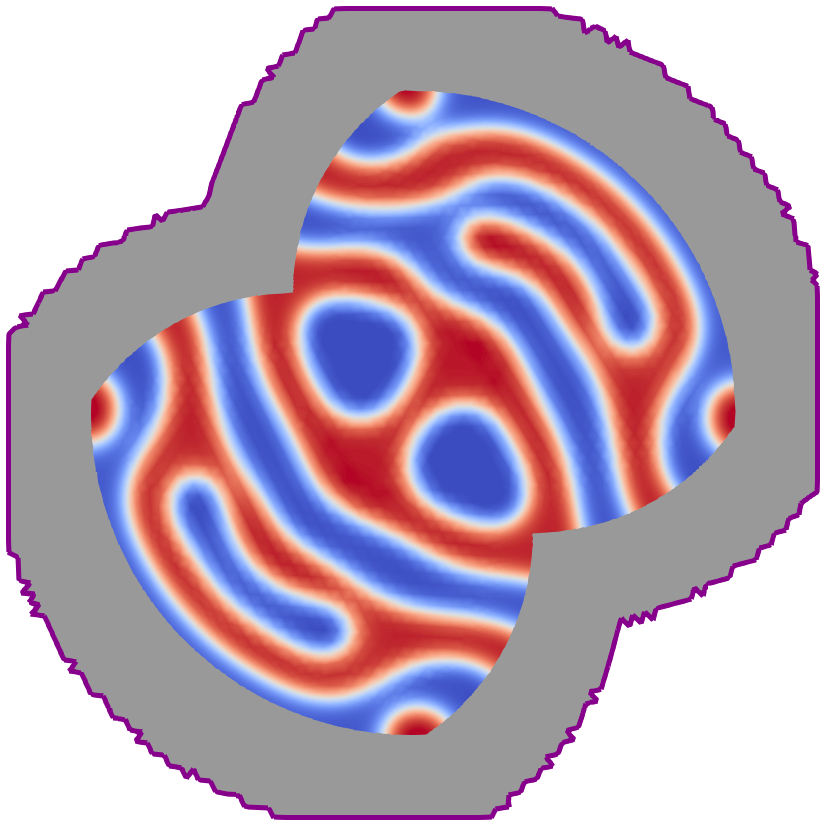
$n=40$
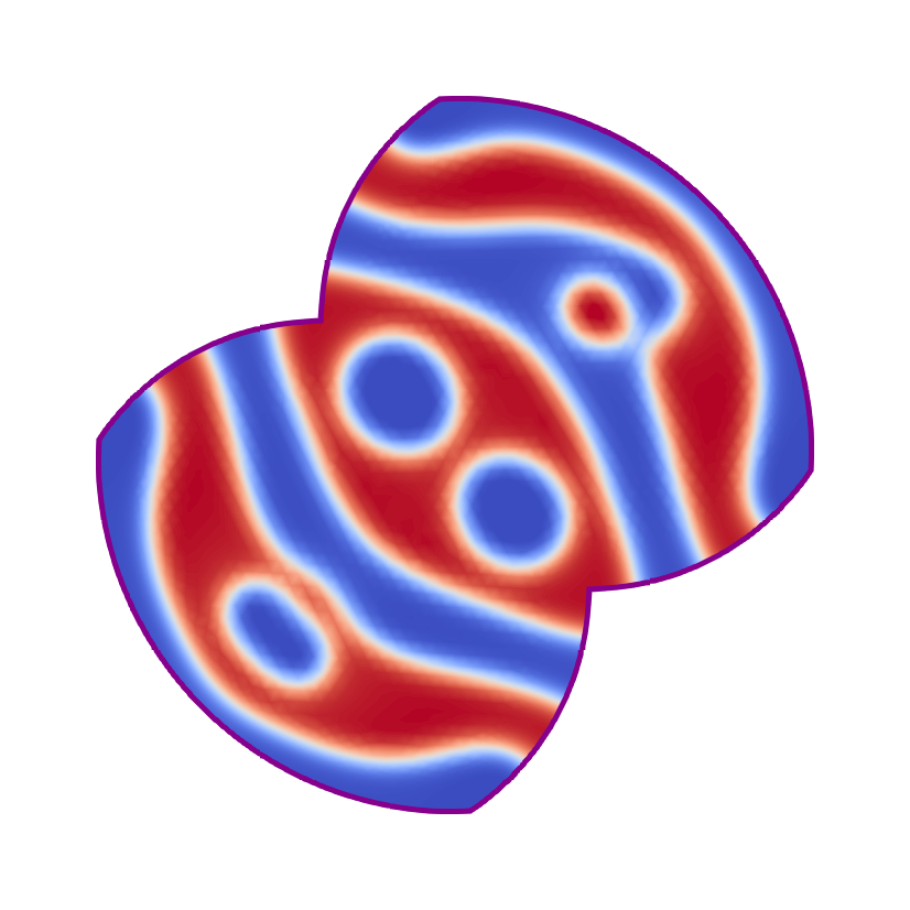
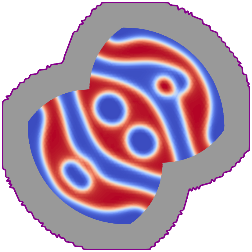
$n=320$

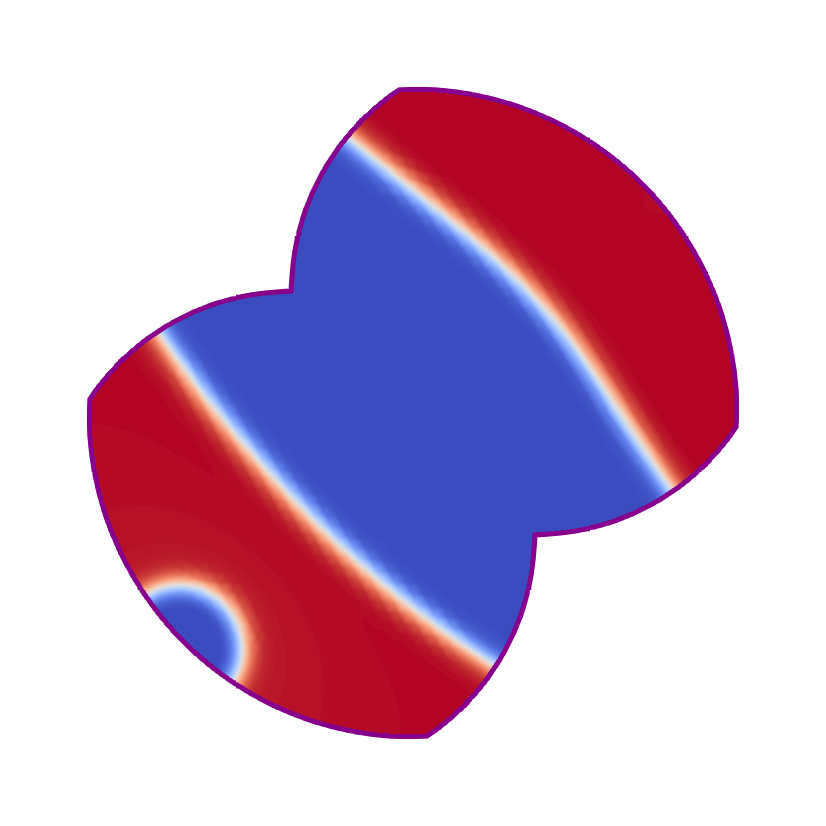
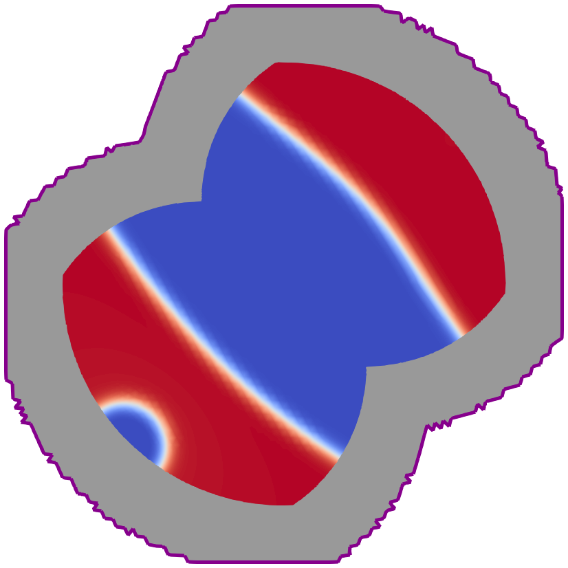
Figure 12: Comparison of approximate solutions to Cahn-Hilliard equation using identical interior meshes

At early time steps ($n=20$) when rapid changes occur, and during later time steps ($n=320$) when the concentration has settled, we observe no difference between the fitted and Diffuse Domain methods.

We can also compare the energy of the system,

$$E(c)=\int_{\Omega{}}{\frac{\lambda}{2}|\nabla c|^{2}+f(c)\;dx}.$$ (39)

The results for both Diffuse Domain approaches are identical so, in Figure 13 we plot just NSDDM. This displays the accuracy of the Diffuse Domain approach.

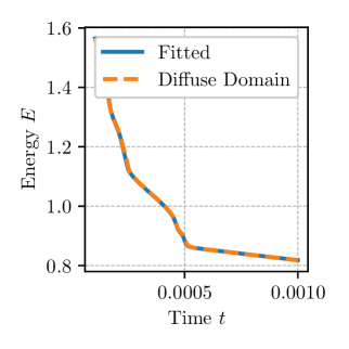
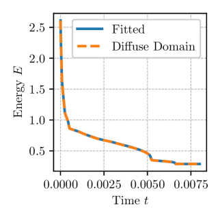
Figure 13: Comparison of computed energy for Cahn-Hilliard problem for Diffuse Domain methods and fitted mesh

6.4 Linear Elasticity

In this example we want to test the implementation of mixed boundaries. Small elasticity deformation of a cantilever beam under gravity is described by

$$-\nabla\cdot\sigma(u)=\left(0,\frac{-9.8}{\rho}\right)^{T}\quad\text{ in }\Omega{},$$ (40a)

$$u =0\text{ on }\partial\Omega{}{}_{D},$$ (40b)

$$\sigma\cdot n =0\text{ on }\partial\Omega{}{}\setminus\partial\Omega{}{}_{D}.$$ (40c)

For linear elasticity [20] the stress tensor is given by

$$\sigma(u)=\lambda(\nabla u+\nabla u^{T})+\mu(\nabla\cdot u)I,$$ (41)

where we use $\mu=0.1$ $\lambda=1$, $\rho=1000$. The beam is free to move under its own weight, except for one side given by $\partial\Omega{}{}_{D}$ where the beam is fixed in place, We will use the domain given by the SDF from Listings 4. This means $\partial\Omega{}{}_{1}$ will be the boundary intersection of the balls with the names left and bounding.

The results in 14 are essentially identical. It is clear that the left boundary has not moved, while the rest has deformed. Therefore, this demonstrates the ability of ddfem to handle both Dirichlet and flux boundaries simultaneously.

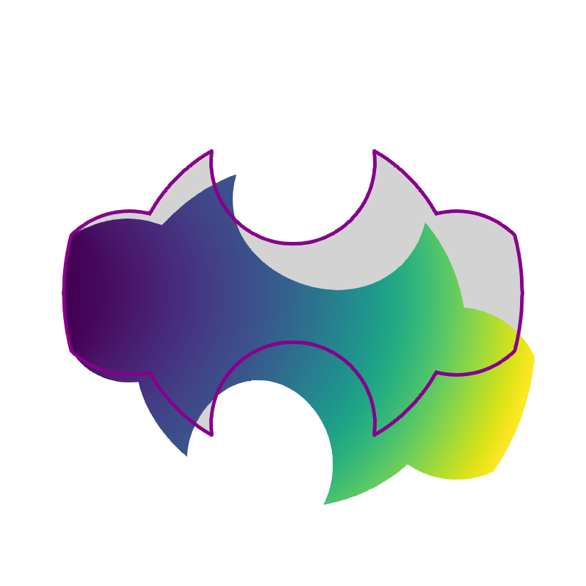
(a) Fitted

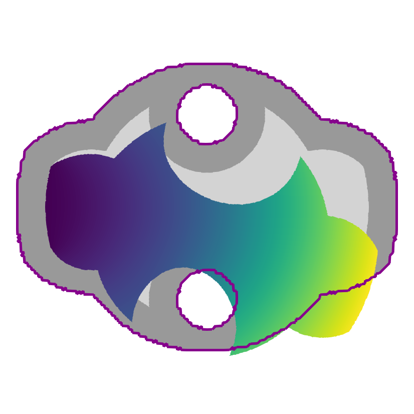
(b) DDM1

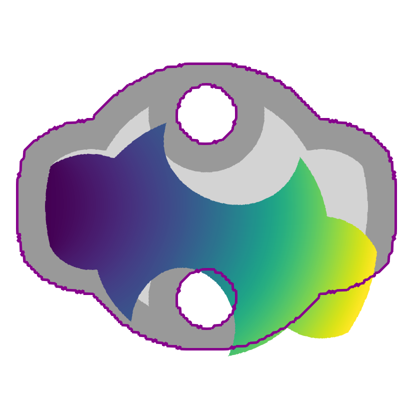
(c) Mix0DDM

Figure 14: Approximate solutions to the linear elasticity problem; the computation domain is show with shades of grey and the problem domain has been warped to show the displacement

6.5 3D Hyperelasticity

We are currently investigating 3D problems for stability of Diffuse Domain methods, and to optimise computational performance. The ddfem.geometry subpackage contains two options to extended 2D SDFs to create 3D SDFs, from the operator classes ddfem.geometry.Extrusion, ddfem.geometry.Revolution. Starting with the domain from Listings 6, we extrude using the Python below to create a domain of a complex beam.

⬇

omega3D = omega.extrude(3.2)

We will use a compressible neo-Hookean model [43] given by the free-energy potential

$$\psi(F)=\frac{\mu}{2}\left(I_{1}-3-2\ln{J}\right)+\frac{\lambda}{2}(J-1)^{2},$$ (42)

where $I_{1}=\operatorname{tr}{F^{T}F}$, $J=\det{F}$, with the deformation gradient $F(U)=I+\nabla U$. The coefficients

$$\lambda =\frac{E\nu}{(1+\nu)(1-2\nu)}, \mu =\frac{E}{2(1+\nu)},$$ (43)

defined by the Young’s modulus $E=1e4$, Poisson’s ration $\nu=0.4$. This gives the Piola-Kirchhoff stress $P(u)=\frac{\partial\psi(F)}{\partial F}$. We define the problem

$$-\nabla\cdot P(u)=\left(0,0,0\right)^{T}\quad\text{ in }\Omega{},$$ (44a)

$$P(u) =\left(0,0,0\right)^{T}\text{ on }\partial\Omega{}{}_{\text{bot}}, P(u) =R(x,\theta)\text{ on }\partial\Omega{}{}_{\text{top}}.$$ (44b)

The domain will only be extended around the complex boundaries, so the flat faces on the end of the beam will match the extended domain. The boundary $\partial\Omega{}{}_{\text{bot}}$ fixes the face, and the boundary $\partial\Omega{}{}_{\text{top}}$ is rotated by angle $\theta$ given by,

$$R(x,\theta)=\begin{pmatrix}\cos\theta&\sin\theta&0\\ -\sin\theta&\cos\theta&0\\ 0&0&1\end{pmatrix}x-x.$$ (45)

An example of the results is shown in Listings 15, both Diffuse Domain methods produce similar results.

	DDM1	NSDDM
$\theta=\frac{\pi}{2}$
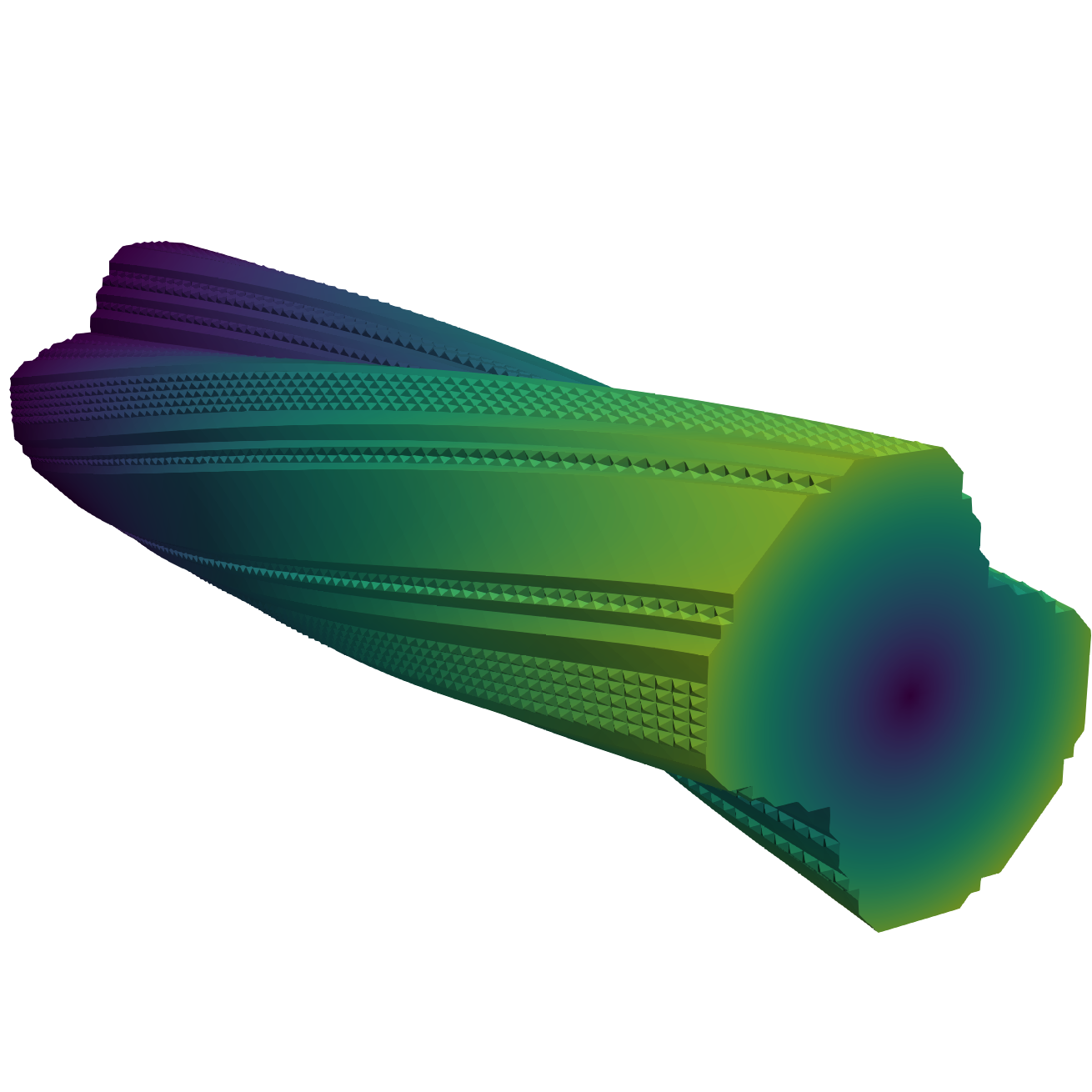
$\theta=\pi$

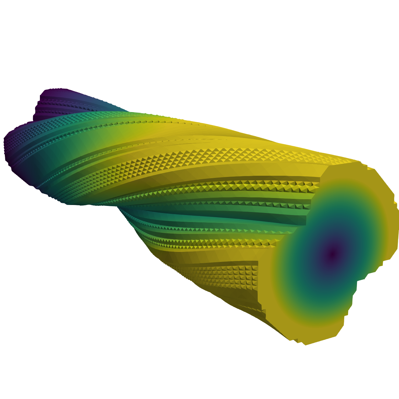
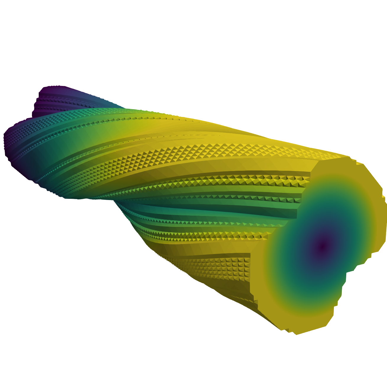
Figure 15: The problem domain has been warped to show the approximate solutions for displacement to the 3D hyperelasticity problem

7 Conclusion

In this paper we have presented the ddfem Python module which allows the easily utilise of the Diffuse Domain method for solving a wide range of PDEs on complex domains. We provide ways to define the domain using SDFs and constructive solid geometry. Then given a standard model class, a transformer is able to apply the chosen Diffuse Domain approach. We have built up the key features and proposed a way to handle mixed boundary condition types. This implementation was then applied to elasticity, reaction-diffusion-advection, Cahn-Hilliard, and compared to a traditional fitted mesh. We could see the Diffuse Domain methods can provide an accurate approximate solution to complex domains, and the added terms for the different boundary conditions are combined correctly for each region.

Noticeable area for us to develop is to remove the limitation of the type of boundary conditions for a system model. Furthermore, a possible extension to the ddfem.geometry subpackage would be to extend this construction scheme to generate SDFs by creating a closed loop from a series of line segments, arcs, and Bézier segments. This would produce a perfect SDF by taking the cross product of each segment. Also, implementing a marching cubes algorithm would provide the ability to generate a SDF from an image.

In future work, we plan to develop our Mix0DDM and NSDDM methods, and provide analysis on their convergence and stability. Including the effects of Mix0DDM with fully flux boundary conditions. Additionally, we are in the process of exploring more time dependent problems with moving domains, and nonlinear problems, including incompressible and compressible fluid flow.

Declarations

*Funding Luke Benfield is supported by the Warwick Mathematics Institute Centre for Doctoral Training, and gratefully acknowledges funding from the University of Warwick.

*Conflict of interest The authors declare no competing interests.

*Data availability The source code for the numerical experiments is available at https://gitlab.dune-project.org/dune-fem/ddfem. A bash script is provided to run all experiments with the same parameters as shown here.

*Code availability All code was implemented in Python using UFL [35], and Dune-Fem [36] for solving PDEs. Utilising Gmsh [41] and Dune-ALUGrid [44] for generating meshes. The source code for the package, and experiments of this article are available at https://gitlab.dune-project.org/dune-fem/ddfem.

*Authors’ contributions Luke Benfield developed the Diffuse Domain implementation, and prepared the first draft of the manuscript. Andreas Dedner contributed to the package development, experiment design, and provided extensive feedback and suggestions for the manuscript. Both authors reviewed and approved the final version.

References

- \bibcommenthead
- Glowinski et al. [1996] Glowinski, R., Pan, T.W., Wells Jr., R.O., Zhou, X.: Wavelet and finite element solutions for the neumann problem using fictitious domains. Journal of Computational Physics 126(1), 40–51 (1996) https://doi.org/10.1006/jcph.1996.0118
- Ramière et al. [2007] Ramière, I., Angot, P., Belliard, M.: A general fictitious domain method with immersed jumps and multilevel nested structured meshes. Journal of Computational Physics 225(2), 1347–1387 (2007) https://doi.org/%****␣ddfem.bbl␣Line␣75␣****10.1016/j.jcp.2007.01.026
- Vos et al. [2008] Vos, P.E.J., Loon, R., Sherwin, S.J.: A comparison of fictitious domain methods appropriate for spectral/hp element discretisations. Computer Method (25-28), 2275–2289 (2008) https://doi.org/10.1016/j.cma.2007.11.023
- Parussini and Pediroda [2009] Parussini, L., Pediroda, V.: Fictitious domain approach with hp-finite element approximation for incompressible fluid flow. Journal of Computational Physics 228(10), 3891–3910 (2009) https://doi.org/10.1016/j.jcp.2009.02.019
- LeVeque and Li [1994] LeVeque, R.J., Li, Z.: The immersed interface method for elliptic equations with discontinuous coefficients and singular sources. SIAM Journal on Numerical Analysis 31(4), 1019–1044 (1994) https://doi.org/10.1137/0731054
- de Prenter et al. [2023] Prenter, F., Verhoosel, C.V., Brummelen, E.H., Larson, M.G., Badia, S.: Stability and conditioning of immersed finite element methods: analysis and remedies. Archives of Computational Methods in Engineering 30(6), 3617–3656 (2023) https://doi.org/10.1007/s11831-023-09913-0
- Griffith and Patankar [2020] Griffith, B.E., Patankar, N.A.: Immersed methods for fluid-structure interaction. Annual Review of Fluid Mechanics 52(1), 421–448 (2020) https://doi.org/10.1146/annurev-fluid-010719-060228
- Fries and Belytschko [2010] Fries, T.-P., Belytschko, T.: The extended/generalized finite element method: An overview of the method and its applications. International Journal for Numerical Methods in Engineering 84(3), 253–304 (2010) https://doi.org/10.1002/nme.2914
- Ji et al. [2006] Ji, H., Lien, F.-S., Yee, E.: An efficient second-order accurate cut-cell method for solving the variable coefficient poisson equation with jump conditions on irregular domains. International Journal for Numerical Methods in Fluids 52(7), 723–748 (2006) https://doi.org/10.1002/fld.1199
- Macklin and Lowengrub [2008] Macklin, P., Lowengrub, J.S.: A new ghost cell/level set method for moving boundary problems: Application to tumor growth. Journal of Scientific Computing 35(2-3), 266–299 (2008) https://doi.org/%****␣ddfem.bbl␣Line␣200␣****10.1007/s10915-008-9190-z
- Kockelkoren et al. [2003] Kockelkoren, J., Levine, H., Rappel, W.-J.: Computational approach for modeling intra- and extracellular dynamics. Physical Review E 68(3), 37–702 (2003) https://doi.org/10.1103/physreve.68.037702
- Li et al. [2009] Li, X., Lowengrub, J., Ratz, A., Voigt, A.: Solving pdes in complex geometries: A diffuse domain approach. Communications in Mathematical Sciences 7(1), 81–107 (2009) https://doi.org/10.4310/cms.2009.v7.n1.a4
- Lervåg and Lowengrub [2015] Lervåg, K.Y., Lowengrub, J.: Analysis of the diffuse-domain method for solving pdes in complex geometries. Communications in mathematical sciences 13(6), 1473–1500 (2015) https://doi.org/10.4310/CMS.2015.v13.n6.a6
- Franz et al. [2012] Franz, S., Roos, H.-G., Gärtner, R., Voigt, A.: A note on the convergence analysis of a diffuse-domain approach. Computational Methods in Applied Mathematics 12(2), 153–167 (2012) https://doi.org/10.2478/cmam-2012-0017
- Burger et al. [2015] Burger, M., Elvetun, O.L., Schlottbom, M.: Analysis of the diffuse domain method for second order elliptic boundary value problems. Foundations of Computational Mathematics 17(3), 627–674 (2015) https://doi.org/10.1007/s10208-015-9292-6
- Schlottbom [2016] Schlottbom, M.: Error analysis of a diffuse interface method for elliptic problems with dirichlet boundary conditions. Applied Numerical Mathematics 109, 109–122 (2016) https://doi.org/10.1016/j.apnum.2016.06.005
- Rätz and Voigt [2006] Rätz, A., Voigt, A.: Pde’s on surfaces - a diffuse interface approach. Communications in Mathematical Sciences 4(3), 575–590 (2006) https://doi.org/10.4310/cms.2006.v4.n3.a5
- Teigen et al. [2009] Teigen, K.E., Li, X., Lowengrub, J., Wang, F., Voigt, A.: A diffuse-interface approach for modelling transport, diffusion and adsorption/desorption of material quantities on a deformable interface. Communications in Mathematical Sciences 7(4), 1009–1037 (2009) https://doi.org/%****␣ddfem.bbl␣Line␣325␣****10.4310/cms.2009.v7.n4.a10 PMCID:PMC3046400
- Abels et al. [2015] Abels, H., Lam, K.F., Stinner, B.: Analysis of the diffuse domain approach for a bulk-surface coupled pde system. SIAM Journal on Mathematical Analysis 47(5), 3687–3725 (2015) https://doi.org/10.1137/15m1009093
- Aland et al. [2012] Aland, S., Landsberg, C., Müller, R., Stenger, F., Bobeth, M., Langheinrich, A.C., Voigt, A.: Adaptive diffuse domain approach for calculating mechanically induced deformation of trabecular bone. Computer Methods in Biomechanics and Biomedical Engineering 17(1), 31–38 (2012) https://doi.org/10.1080/10255842.2012.654606
- Nguyen et al. [2017a] Nguyen, L.H., Stoter, S.K.F., Ruess, M., Sanchez Uribe, M.A., Schillinger, D.: The diffuse nitsche method: Dirichlet constraints on phase-field boundaries. International Journal for Numerical Methods in Engineering 113(4), 601–633 (2017) https://doi.org/10.1002/nme.5628
- Nguyen et al. [2017b] Nguyen, L., Stoter, S., Baum, T., Kirschke, J., Ruess, M., Yosibash, Z., Schillinger, D.: Phase-field boundary conditions for the voxel finite cell method: Surface-free stress analysis of ct-based bone structures. International Journal for Numerical Methods in Biomedical Engineering 33(12) (2017) https://doi.org/10.1002/cnm.2880
- Chen and Lowengrub [2014] Chen, Y., Lowengrub, J.S.: Tumor growth in complex, evolving microenvironmental geometries: A diffuse domain approach. Journal of Theoretical Biology 361, 14–30 (2014) https://doi.org/10.1016/j.jtbi.2014.06.024
- Chadwick et al. [2018] Chadwick, A.F., Stewart, J.A., Enrique, R.A., Du, S., Thornton, K.: Numerical modeling of localized corrosion using phase-field and smoothed boundary methods. Journal of The Electrochemical Society 165(10), 633–646 (2018) https://doi.org/10.1149/2.0701810jes
- Rätz [2016] Rätz, A.: Diffuse-interface approximations of osmosis free boundary problems. SIAM Journal on Applied Mathematics 76(3), 910–929 (2016) https://doi.org/10.1137/15m1025001
- Aland et al. [2010] Aland, S., Lowengrub, J., Voigt, A.: Two-phase flow in complex geometries: A diffuse domain approach. Computer Modeling in Engineering & Sciences 57(1), 77–106 (2010) https://doi.org/10.3970/cmes.2010.057.077
- Guo et al. [2021] Guo, Z., Yu, F., Lin, P., Wise, S., Lowengrub, J.: A diffuse domain method for two-phase flows with large density ratio in complex geometries. Journal of Fluid Mechanics 907 (2021) https://doi.org/10.1017/jfm.2020.790
- Teigen et al. [2011] Teigen, K.E., Song, P., Lowengrub, J., Voigt, A.: A diffuse-interface method for two-phase flows with soluble surfactants. Journal of Computational Physics 230(2), 375–393 (2011) https://doi.org/10.1016/j.jcp.2010.09.020
- Bukač et al. [2023] Bukač, M., Muha, B., Salgado, A.J.: Analysis of a diffuse interface method for the stokes-darcy coupled problem. ESAIM: Mathematical Modelling and Numerical Analysis 57(5), 2623–2658 (2023) https://doi.org/10.1051/m2an/2023062
- Termuhlen et al. [2022] Termuhlen, R., Fitzmaurice, K., Yu, H.-C.: Smoothed boundary method for simulating incompressible flow in complex geometries. Computer Methods in Applied Mechanics and Engineering 399, 115312 (2022) https://doi.org/10.1016/j.cma.2022.115312
- Aland et al. [2012] Aland, S., Lowengrub, J., Voigt, A.: Particles at fluid-fluid interfaces: A new navier-stokes-cahn-hilliard surface- phase-field-crystal model. Physical Review E 86(4), 046321 (2012) https://doi.org/10.1103/physreve.86.046321
- Yu et al. [2020] Yu, F., Guo, Z., Lowengrub, J.: Higher-order accurate diffuse-domain methods for partial differential equations with dirichlet boundary conditions in complex, evolving geometries. Journal of Computational Physics 406, 109–174 (2020) https://doi.org/10.1016/j.jcp.2019.109174
- Yu et al. [2009] Yu, H.-C., Chen, H.-Y., Thornton, K.: Smoothed boundary method for solving partial differential equations with general boundary conditions on complex boundaries (2009) arXiv:0912.1288 [math.PH]
- Monte et al. [2022] Monte, E.J., Lowman, J., Abukhdeir, N.M.: A diffuse interface method for simulation-based screening of heat transfer processes with complex geometries. The Canadian Journal of Chemical Engineering 100(10), 3047–3062 (2022) https://doi.org/10.1002/cjce.24320
- Alnæs et al. [2014] Alnæs, M.S., Logg, A., Ølgaard, K.B., Rognes, M.E., Wells, G.N.: Unified form language: A domain-specific language for weak formulations of partial differential equations. ACM Transactions on Mathematical Software 40(2), 1–37 (2014) https://doi.org/10.1145/2566630
- Dedner et al. [2020] Dedner, A., Nolte, M., Klöfkorn, R.: Python Bindings for the DUNE-FEM module (2020). https://doi.org/10.5281/zenodo.3706994
- Baratta et al. [2023] Baratta, I.A., Dean, J.P., Dokken, J.S., Habera, M., Hale, J.S., Richardson, C.N., Rognes, M.E., Scroggs, M.W., Sime, N., Wells, G.N.: DOLFINx: The next generation FEniCS problem solving environment. Zenodo (2023). https://doi.org/10.5281/ZENODO.10447666
- Ham et al. [2023] Ham, D.A., Kelly, P.H.J., Mitchell, L., Cotter, C.J., Kirby, R.C., Sagiyama, K., Bouziani, N., Vorderwuelbecke, S., Gregory, T.J., Betteridge, J., Shapero, D.R., Nixon-Hill, R.W., Ward, C.J., Farrell, P.E., Brubeck, P.D., Marsden, I., Gibson, T.H., Homolya, M., Sun, T., McRae, A.T.T., Luporini, F., Gregory, A., Lange, M., Funke, S.W., Rathgeber, F., Bercea, G.-T., Markall, G.R.: Firedrake User Manual. (2023). https://doi.org/%****␣ddfem.bbl␣Line␣675␣****10.25561/104839
- Dedner and Klöfkorn [2022] Dedner, A., Klöfkorn, R.: Extendible and efficient python framework for solving evolution equations with stabilized discontinuous galerkin methods. Communications on Applied Mathematics and Computation 4, 657–696 (2022) https://doi.org/10.1007/s42967-021-00134-5
- Houston and Sime [2018] Houston, P., Sime, N.: Automatic symbolic computation for discontinuous galerkin finite element methods. SIAM Journal on Scientific Computing 40(3), 327–357 (2018) https://doi.org/10.1137/17m1129751
- Geuzaine and Remacle [2009] Geuzaine, C., Remacle, J.-F.: Gmsh: A 3-d finite element mesh generator with built-in pre- and post-processing facilities. International Journal for Numerical Methods in Engineering 79(11), 1309–1331 (2009) https://doi.org/10.1002/nme.2579
- Quilez [2020] Quilez, I.: 2D Distance Functions. https://iquilezles.org/articles/distfunctions2d/ (2020)
- Bleyer [2024] Bleyer, J.: Numerical tours of Computational Mechanics with FEniCSx. Zenodo. Version: v0.1 (2024). https://doi.org/10.5281/zenodo.10470942
- Alkämper et al. [2016] Alkämper, M., Dedner, A., Klöfkorn, R., Nolte, M.: The dune-alugrid module. 4(1), 1–28 (2016) https://doi.org/10.11588/ANS.2016.1.23252