Graph Neural Networks Powered by Encoder Embedding for Improved Node Learning

Abstract

Graph neural networks (GNNs) have emerged as a powerful framework for a wide range of node-level graph learning tasks. However, their performance is often constrained by reliance on random or minimally informed initial feature representations, which can lead to slow convergence and suboptimal solutions. In this paper, we leverage a statistically grounded method, one-hot graph encoder embedding (GEE), to generate high-quality initial node features that enhance the end-to-end training of GNNs. We refer to this integrated framework as the GEE-powered GNN (GG), and demonstrate its effectiveness through extensive simulations and real-world experiments across both unsupervised and supervised settings. In node clustering, GG consistently achieves state-of-the-art performance, ranking first across all evaluated real-world datasets, while exhibiting faster convergence compared to the standard GNN. For node classification, we further propose an enhanced variant, GG-C, which concatenates the outputs of GG and GEE and outperforms competing baselines. These results confirm the importance of principled, structure-aware feature initialization in realizing the full potential of GNNs.

I Introduction

Graphs are ubiquitous data structures that naturally capture relationships between objects, playing a crucial role in domains such as social networks, recommendation systems, and biological networks. Motivated by the pressing need to effectively learn from such graph-structured data, graph neural networks (GNNs) [1, 2, 3, 4, 5] have collected significant interests in recent years and delivered promising results on link prediction, node clustering, and node classification [6, 7, 8].

Despite much progress in GNN research [9, 10, 11, 12], the initialization of node embeddings is a critical yet underexplored aspect. Existing GNNs commonly rely on either raw node attributes or simplistic initialization schemes, such as degree-based features, random vectors, or identity matrices (when explicit features are unavailable). However, these arbitrary or minimally informed initializations frequently fail to capture the rich structural information encoded in the graph topology. As a result, they may lead to slower convergence, greater sensitivity to hyperparameter choices, and suboptimal solutions during training. This limitation is particularly important in tasks like node clustering, which depend heavily on the quality of node representations. It can also affect node classification, where a well-informed initialization can significantly accelerate the learning process.

A promising direction for addressing the limitations of current GNN initialization schemes is to leverage more structured and informative initial node embeddings. To that end, one-hot graph encoder embedding (GEE)[13] offers a lightning-fast and effective method for encoding graph nodes. This simple yet powerful technique can process graphs with millions of edges in seconds while producing embeddings that are both statistically principled and provably convergent to latent positions under random graph models. GEE has been successfully applied to a variety of graph learning tasks, including node classification, clustering, multi-graph embedding, latent community detection, and outlier detection[14, 15, 16, 17, 18].

While GEE provides fast, high-quality embeddings that capture global structural information and often performs competitively, it can occasionally fall short in capturing the intricate patterns and entangled inter-class relationships in complicated real-world networks. On the other hand, neural-network based approaches excel at refining local patterns and capturing complex nonlinear structures, even when initialized with random or uninformative features.

This insight suggests a natural and effective integration of the two approaches. In this paper, we propose and evaluate the GEE-powered GNN (GG), which incorporates GEE-generated embedding as the initial node features within the standard Graph Convolutional Network (GCN) architecture [1, 2], applied to both clustering and classification tasks. In the node clustering task, GG demonstrates not only faster convergence but also consistently superior performance compared to the baseline GNN with randomized initialization, ranking first across all 16 real-world datasets evaluated. For node classification, we further develop a concatenated variant, GG-C, which demonstrates excellent performance across a wide range of training set sizes—from as low as $5\%$ (essentially a semi-supervised setting) to $50\%$ of the nodes used for training.

The remainder of the paper is organized as follows: Section II introduces our implementations of the GG method based on GNN and GEE. Section III provides an intuitive theoretical motivation for GG using embedding visualizations and convergence rate analyses. Section IV presents clustering performance results on both simulated and real-world datasets. Section V describes the classification adaptation of GG-C, which differs from the clustering setting due to label availability and changes in the learning objective. Section VI reports classification results under various training percentages on both synthetic and real data. Additional experiments are provided in the supplementary material. The source code of our method is available on Github.

II Clustering Method

II-A GNN

The architecture considered in this paper utilizes the graph convolution network with residual skip connections [19] and employs the loss of deep modularity networks (DMoN)[8] to enhance community structure preservation.

II-A1 GCN

The layer-wise propagation rule of GCN is defined as follows:

$$Z^{(l+1)}=\sigma\left(\tilde{D}^{-\frac{1}{2}}\tilde{A}\tilde{D}^{-\frac{1}{2}}Z^{(l)}W^{(l)}\right).$$

Here, $\tilde{A}=A+I_{n}$ is the adjacency matrix with added self-connections, where $A$ is the original adjacency matrix, $I_{n}\in{R}^{n\times n}$ is the identity matrix and $n$ is the number of nodes. The degree matrix $\tilde{D}$ of $\tilde{A}$ is defined as $\tilde{D}_{ii}=\sum_{j}\tilde{A}_{ij}$. $W^{(l)}$ represents the trainable weight matrix for the $l$-th layer, and $\sigma(\cdot)$ denotes the activation function, which in this case is the ReLU function, defined as $\sigma(x)=\max(0,x)$. Finally, $Z^{(l)}\in{R}^{n\times d}$ is the activation matrix in the $l$-th layer, where $Z^{(0)}$ can be either randomized inital embeddings or specific node features. Here, $d$ denotes the embedding dimension, which is set to match the number of clusters $K$.

II-A2 Skip connections

Skip connections add the initial features to the outputs of each GCN layer to obtain the final representation $\hat{Z}$, which can be formulated as:

$$\hat{Z}=\sum_{l=0}^{L}Z^{(l)},$$

where $L=2$ denotes the number of layers. In this way, the network ensures that meaningful information from earlier layers is preserved and leveraged throughout the training process, reducing the risk of feature degradation in deeper layers.

II-A3 DMoN loss

The loss function of DMoN combines spectral modularity maximization with a regularization term to avoid trivial solutions and is formulated as:

$$C=\text{softmax}(\hat{Z}),$$

$$\mathcal{L}_{\text{DMoN}}(C;A)=-\frac{1}{2m}\text{Tr}(C^{\top}BC)+\frac{\sqrt{k}}{n}\left|\left|\sum_{i}C_{i}^{\top}\right|\right|_{F}-1,$$

where $C\in R^{n\times k}$ is the soft community assignment matrix, obtained by applying the softmax function to the GNN output $\hat{Z}$. The adjacency matrix of the graph is denoted as $A$, and $m=\frac{1}{2}\sum_{i,j}A_{ij}$ is the total number of edges. The modularity matrix $B$ is defined as: $B=A-\frac{vv^{\top}}{2m}$, where $v$ represents the degree vector of the graph, computed as: $v=A\mathbf{1}_{n}$, with $\mathbf{1}_{n}\in R^{n}$ being a column vector of ones.

The term $\text{Tr}(C^{\top}BC)$ corresponds to the modularity maximization component, which encourages dense within-class connections while reducing between-class edges. The regularization term $\left|\left|\sum_{i}C_{i}^{\top}\right|\right|_{F}$ computes the Frobenius norm of the aggregated community assignments, thereby preventing trivial solutions by mitigating the collapse of clusters.

II-A4 Prediction

The soft community assignment matrix $C$, derived from the GNN output via a softmax function, serves as a probability matrix. Each node is assigned to the community with the highest probability:

$$\hat{Y}=\text{argmax}(C,\text{dim}=1).$$

To formalize the entire unsupervised GNN pipeline, we encapsulate it as a single function $F^{u}_{GNN}$ that maps the initial features $Z^{(0)}$ and the graph structure $A$ to the final label predictions $\hat{Y}$:

$$\hat{Y}=F^{u}_{GNN}(Z^{(0)},A).$$

In the case of the vanilla GNN, we use a randomized initial embedding $X_{0}$ as the input of $F^{u}_{GNN}$:

$$\hat{Y}_{GNN}=F^{u}_{GNN}(X_{0},A).$$

In our implementation, $X_{0}\in R^{n\times k}$ is initialized using the Xavier uniform initialization, where each embedding element is sampled from $\mathcal{U}\left(-\sqrt{\frac{6}{k+n}},\sqrt{\frac{6}{k+n}}\right)$.

II-B GEE

GEE is an efficient and flexible graph embedding method that can be applied with ground-truth labels, labels generated by other methods, partial labels, or without labels. The core step of supervised GEE is the multiplication of adjacency matrix $A$ with a column-normalized one-hot encoding matrix $W$:

$$Z=AW,\quad W_{ik}=\frac{\mathbb{I}\{\,Y_{i}=k\,\}}{n_{k}},$$ (1)

where $\mathbb{I}(\cdot)$ is the indicator function and $n_{k}=\sum_{j=1}^{n}\mathbb{I}\{Y_{j}=k\}$ is the size of community $k\in[1,K]$.

GEE first converts every node into a scaled one-hot vector: if node $i$ belongs to community $k$, the entry $W_{ik}$ equals $1/n_{k}$; Otherwise, it is $0$. Consequently, each column of $W$ sums up to $1$ and can be interpreted as a probability distribution over the nodes in that community.

Multiplying $A$ by $W$ yields the final embedding matrix $Z$. The $i$-th row $Z_{i}$ summarizes how strongly node $i$ is connected to all $K$ clusters, while the $k$-th column $Z_{\cdot k}$ serves as a ‘prototype’ vector for the community $k$ in the adjacency space.

In the clustering task, we adopt the unsupervised version of GEE. The procedure starts with a random label vector, then repeats:

1. compute node embeddings with the supervised GEE, and

2. run $k$-means on the embeddings to update the labels.

The loop ends when the labels stop changing or when the maximum number of iterations $M$ is reached. Formally, the whole routine can be viewed as a function $F^{u}_{GEE}(A,k,M)$:

$$(\hat{Z}_{GEE},\hat{Y}_{GEE})=F^{u}_{GEE}(A,k,M).$$ (2)

II-C GEE-powered GNN (GG)

We first generate a well-initialized node features $\hat{Z}_{GEE}$ from Eq. (2), and utilize it as the input of the function $F^{u}_{GNN}$ to obtain the predicted label vector $\hat{Y}_{GG}$:

$$\hat{Y}_{GG}=F^{u}_{GNN}(\hat{Z}_{GEE},A).$$

III Theoretical Motivation

Identifying meaningful community structures in graphs is a fundamental task in network analysis. Modularity optimization has emerged as a prominent approach [20], aiming to find partitions that maximize this score. However, directly optimizing modularity presents significant challenges. The problem is NP-hard [21], and its optimization landscape is notoriously ‘rugged,’ characterized by an exponential number of near-optimal partitions [22, 23]. This often leads heuristic search algorithms to converge to local optima that are highly sensitive to initial conditions or node processing order. While subsequent algorithms like Leiden have made strides in guaranteeing well-connected communities [24], the fundamental challenge of navigating this rugged, NP-hard landscape via discrete, heuristic search persists.

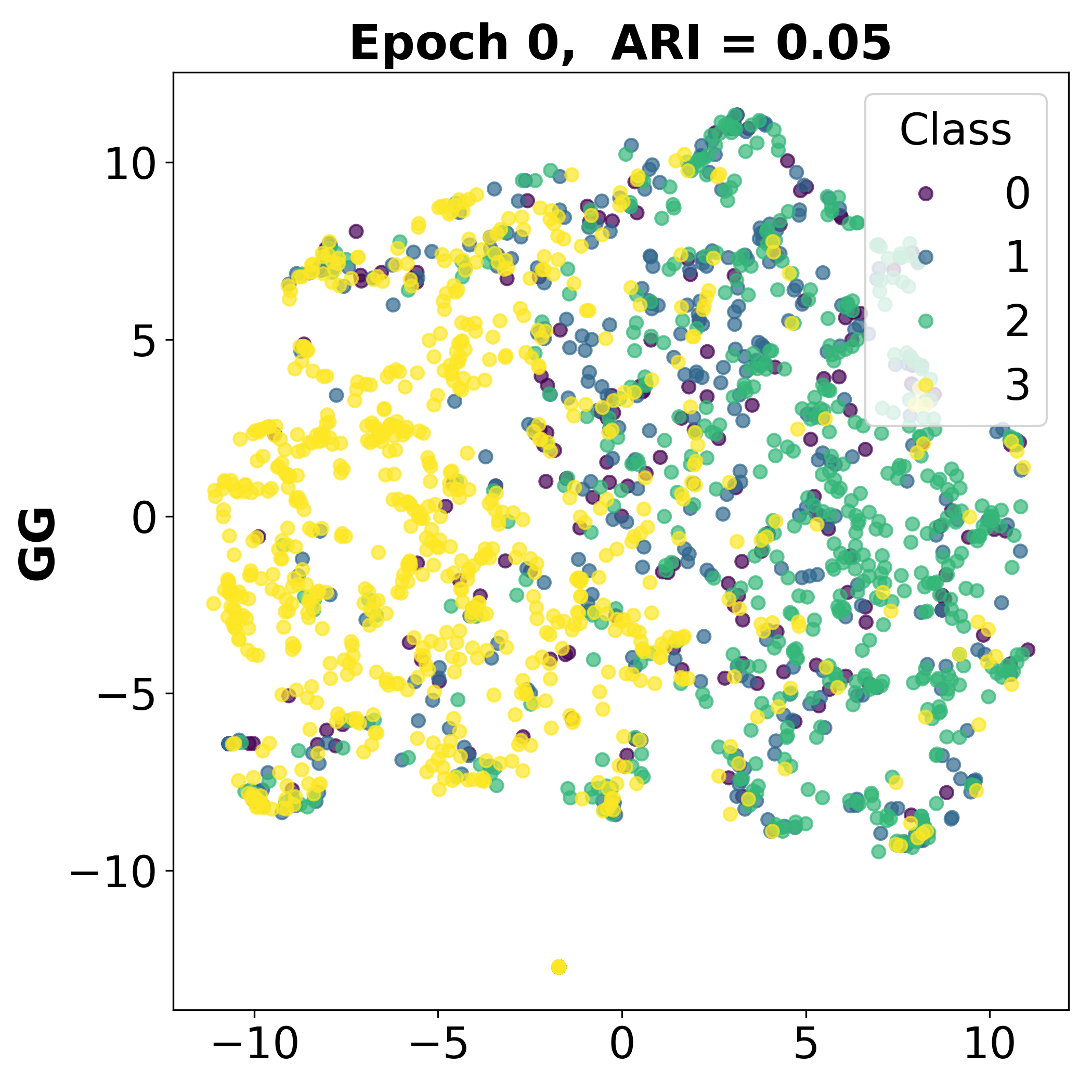
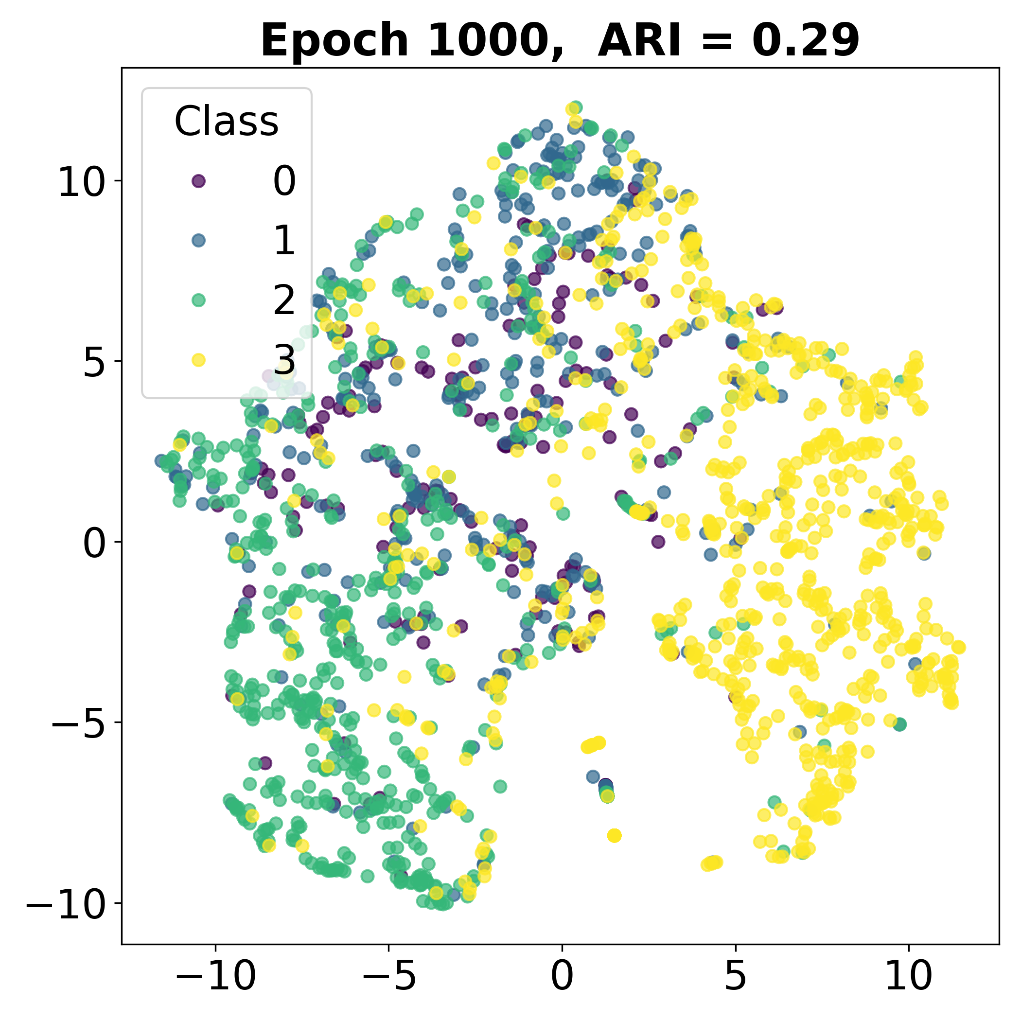
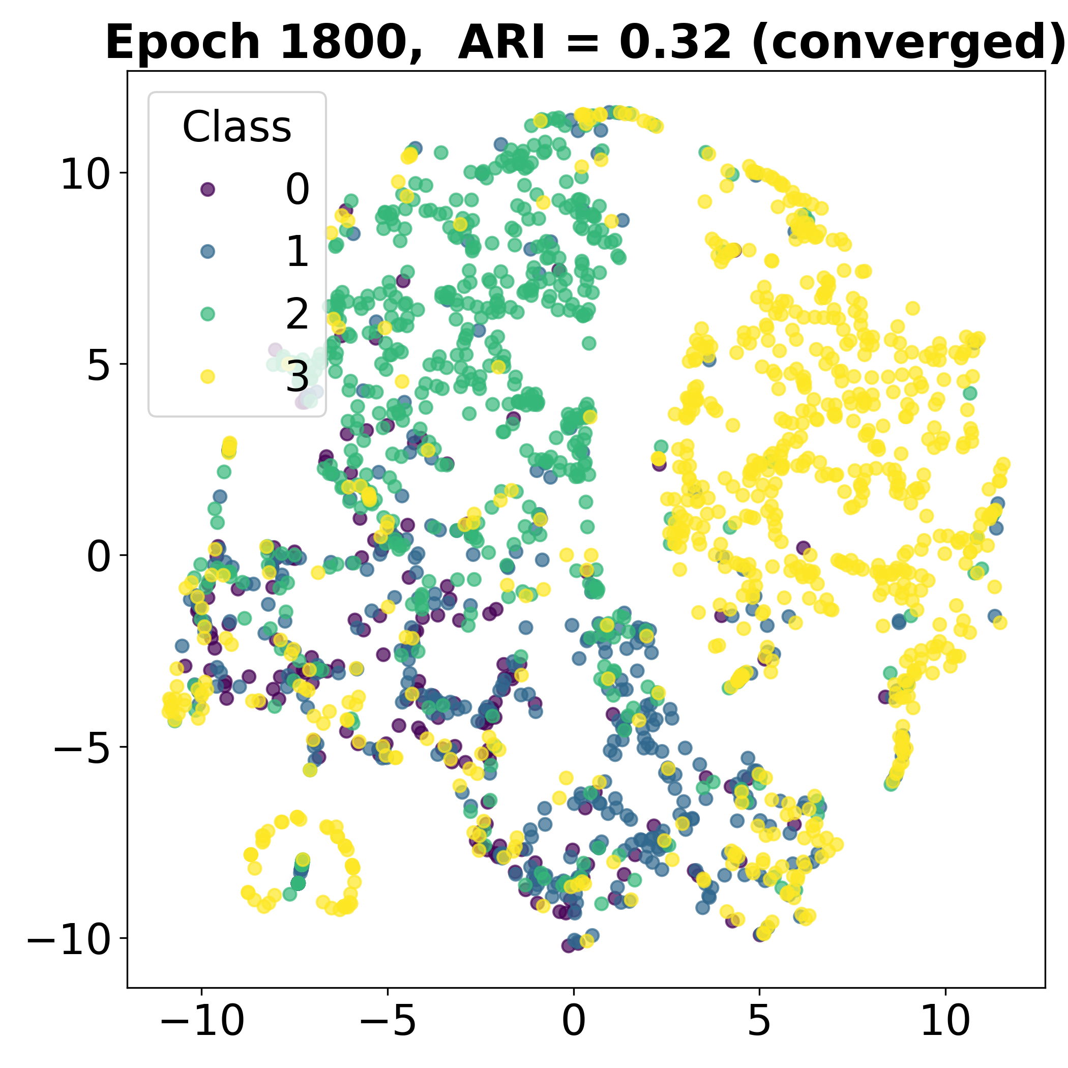
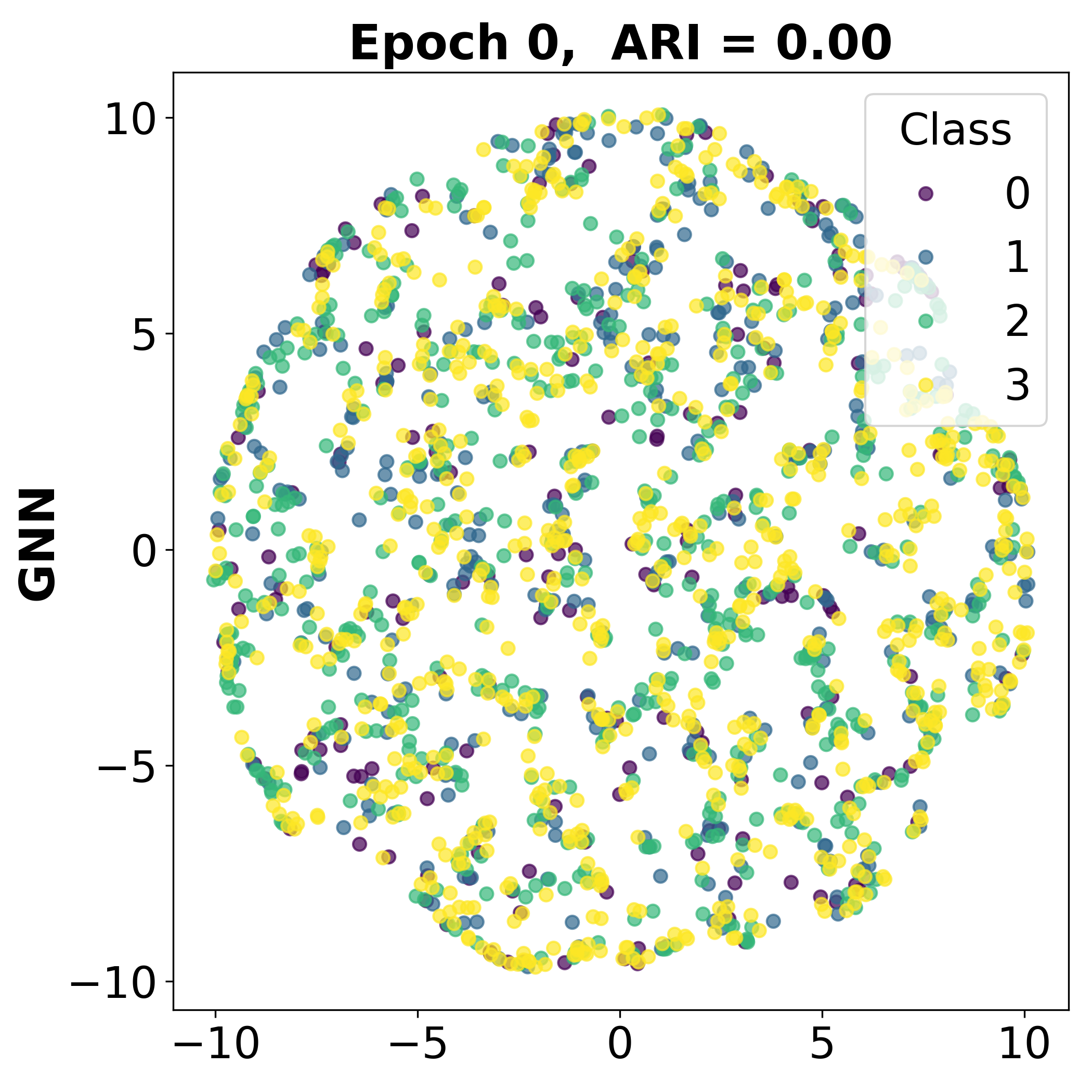
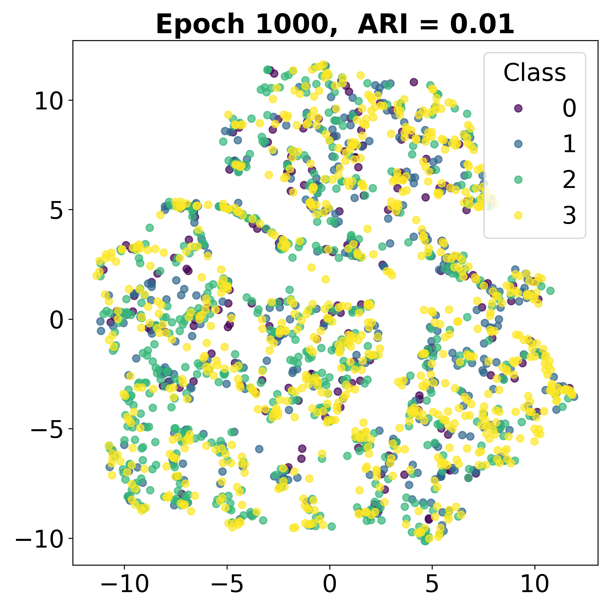
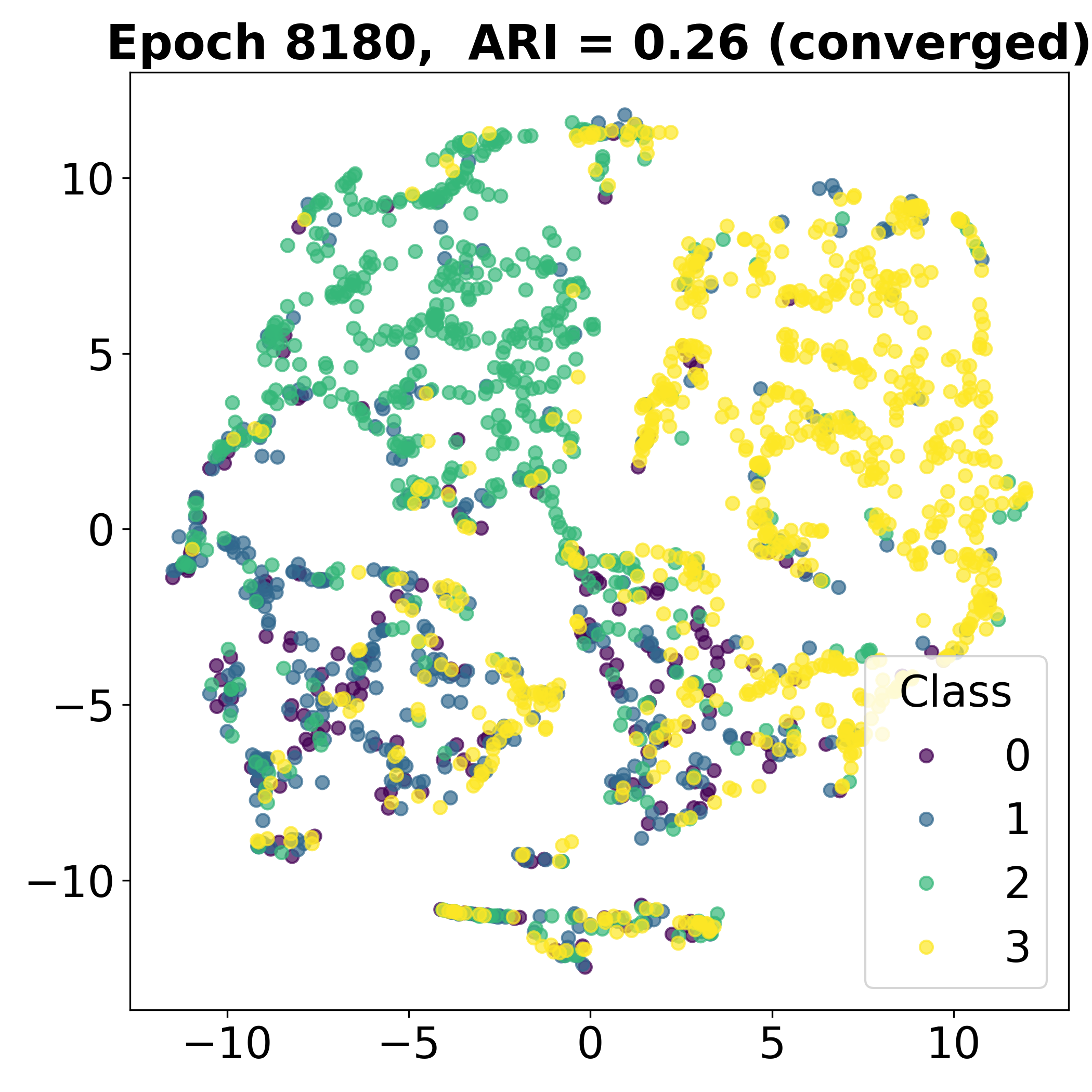
Figure 1: Visualization of Training Dynamics and Clustering Quality. This figure contrasts the training process of our proposed GG (top row) and a vanilla GNN (bottom row) on a Degree-Corrected Stochastic Block Model (DC-SBM) graph (see Subsection IV-A for detailed settings). It demonstrates that GG’s warm-start leads to a better initial state, faster convergence, and a superior final clustering quality. GG begins with a structured embedding (ARI = 0.05) and converges in only 1,800 epochs to a high-quality partition (ARI = 0.32). In contrast, the GNN starts from a random state (ARI $\approx$ 0.00) and requires a much longer training of 8,180 epochs to achieve an inferior result (ARI = 0.26).

This is where a learning-based approach, specifically using GNNs, offers a paradigm shift. Instead of directly searching the discrete space of partitions, a GNN reframes the problem as a continuous optimization task. By training a GNN with a differentiable modularity-style loss, the network learns low-dimensional node embeddings that are inherently optimized for community structure [25, 26, 8]. This learned, continuous representation space effectively ‘smooths out’ the notoriously rugged modularity landscape, making it amenable to gradient-based optimization.

However, even in this smoother landscape, the non-convex nature of the optimization means that the choice of initialization remains critical. This motivates our core proposal: GG, a GNN that is warm-started with embeddings from the statistically consistent GEE, which combines the best of both worlds. The GEE initialization places the GNN in a promising region of the embedding space. From this advantaged starting point, the GNN’s training can fine-tune the representations and converge to markedly superior optima than vanilla GNN that rely on random initializations [1].

To empirically validate this hypothesis, we visualize the evolution of node embeddings for both GG and the vanilla GNN during training on a DC-SBM graph. As illustrated in Figure 1, the impact of our warm-starting strategy is immediately apparent. GG (top row) begins at Epoch 0 with some discernible community structure (ARI = 0.05), visually confirming that it starts in a ”promising region” of the embedding space. Then it rapidly refines this structure, converging in only 1,800 epochs to a high-quality partition with an ARI of 0.32. In comparison, the randomly initialized GNN (bottom row) starts from a completely unstructured state (ARI = 0.00). Its learning trajectory is substantially slower, showing negligible improvement even by Epoch 1000 (ARI = 0.01). Ultimately, it requires a much longer training process (8,180 epochs) to reach a significantly inferior solution (ARI = 0.26).

This side-by-side comparison offers an intuitive justification for our approach. By employing GEE as the initial node feature representation, owing to its statistically grounded formulation and its convergence to latent positions under random graph models [13], the method provides high-quality initial embeddings that capture the global structural properties of the graph. This strong initialization significantly benefits the subsequent neural network optimization process, enabling faster convergence and improved final results. In doing so, it effectively circumvent the challenges posed by the rugged and non-convex optimization landscape typical of GNN training.

IV Clustering Evaluation

To systematically evaluate the performance of the proposed GG method, we conduct experiments on both synthetic and real-world datasets. The evaluation considers two parts: clustering accuracy, where we compare GG against GEE and the vanilla GNN; and running time, focusing on the convergence time difference between GG and the vanilla GNN.

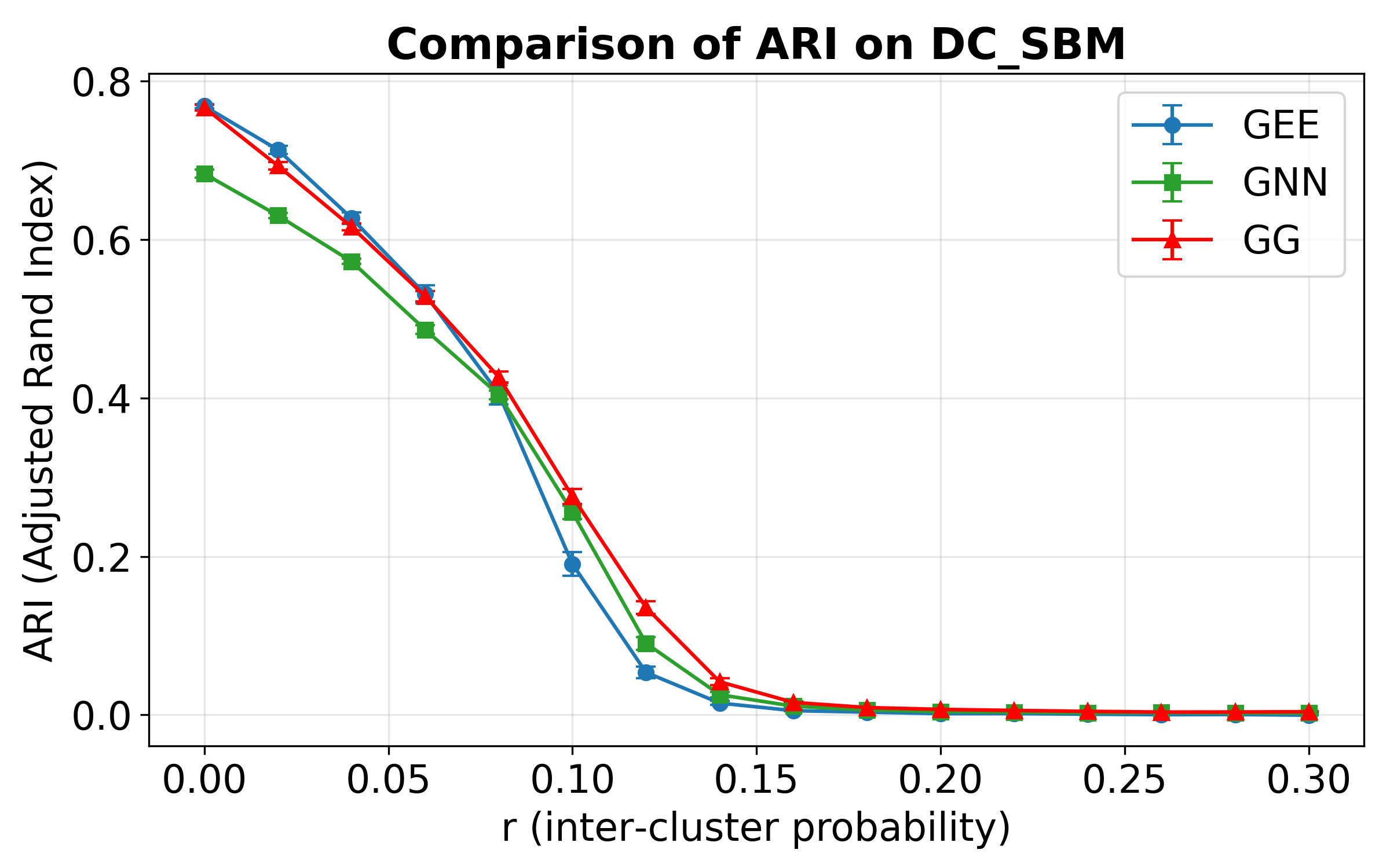
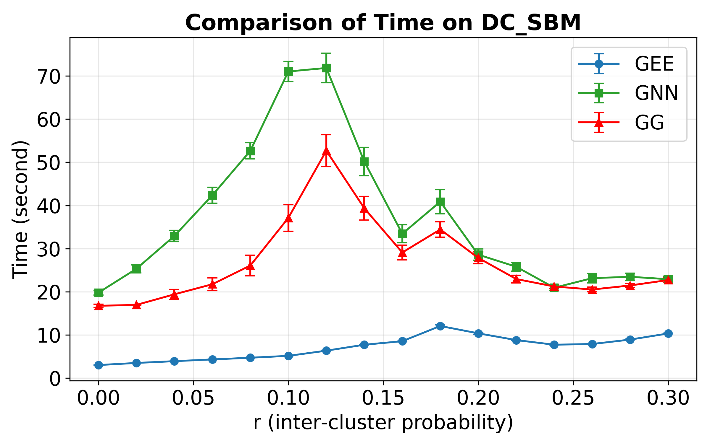
Figure 2: Clustering performance comparison of GEE, GNN and GG on DC-SBM graphs. This figure shows that our proposed GG offers the best trade-off between clustering accuracy (ARI, left) and speed (Time, right). While GEE is fastest, GG matches or surpasses its accuracy, especially on more challenging graphs ($r>0.08$). Compared to the vanilla GNN, GG is both more accurate and substantially faster across all conditions.

For each graph, whether real-world or synthetic, we generate three distinct sets of label predictions: $\hat{Y}_{GEE}$ from GEE, $\hat{Y}_{GNN}$ from a vanilla GNN, and $\hat{Y}_{GG}$ from the proposed GG. We then assess the quality of these predictions against the ground-truth labels using the Adjusted Rand Index (ARI). The ARI measures the similarity between two clusterings, where a score of $1$ indicates a perfect match, and values near $0$ suggest random partitioning.

IV-A Simulation

For simulations, we consider the stochastic block model (SBM) [27] and the degree-corrected SBM (DC-SBM) [28]. Here we present the results on DC-SBM, as it better captures the degree heterogeneity in real-world networks. Results for SBM are available in Appendix.

In DC-SBM, the generative process for an edge between two nodes depends on three components: their community assignments, a shared block probability matrix, and individual degree parameters. First, each node $i$ is assigned to a community, represented by a label $Y_{i}\in\{1,\dots,K\}$. The connectivity between these communities is governed by the block probability matrix $B\in[0,1]^{K\times K}$, where entry $B(k,l)$ specifies the probability of a link between a node in community $k$ and a node in community $l$. The key distinction from the standard SBM is the introduction of a degree parameter $\theta_{i}$ for each node to account for degree heterogeneity.

Combining these elements, the adjacency matrix $A\in\{0,1\}^{n\times n}$ is generated as follows:

$$A_{ij}\sim\text{Bernoulli}\left(\theta_{i}\theta_{j}B(Y_{i},Y_{j})\right)$$

where $A(i,i)=0$ and $A(j,i)=A(i,j)$ to ensure the graph is simple and undirected.

TABLE I: Summary of datasets used in experiments

Dataset	Vertices	Edges	Classes	Community sizes
Cora	2708	5429	7	818, 426, 418, 351
Citeseer	3327	4732	6	701, 668, 596, 590
ACM	3025	13128	3	1061, 999, 965
Chameleon	2277	18050	5	521, 460, 456, 453
DBLP	4057	3528	4	1197, 1109, 1006, 745
EAT	399	203	4	102, 99, 99, 99
UAT	1190	13599	4	299, 297, 297, 297
BAT	131	1074	4	35, 32, 32, 32
KarateClub	34	156	4	13, 12, 5, 4
Email	1005	25571	42	109, 92, 65, 61
Gene	1103	1672	2	613, 490
Industry	219	630	3	133, 44, 42
LastFM	7624	27806	17	1303, 1098, 655, 515
PolBlogs	1490	33433	2	636, 588
Wiki	2405	16523	17	406, 361, 269, 228
TerroristRel	881	8592	3	633, 181, 67

For the experimental setup, the graphs are configured with $n=2000$ nodes and $K=4$ communities. To evaluate model performance under varying degrees of community separability, we fix the intra-community edge probability at $0.3$ while systematically varying the inter-community probability $r$ from $0$ to $0.3$ in increments of $0.02$. To introduce degree heterogeneity, the degree correction parameters $\theta_{i}$ are drawn from a Beta distribution, $\beta(1,4)$. Furthermore, we impose a structural imbalance by setting the community sizes to a ratio of 1:2:3:4, a choice intended to better reflect the skewed community size distributions often found in real-world networks.

To ensure the statistical reliability of our findings across all simulation experiments (including SBM in Appendix), we conduct 50 independent runs for each graph generated at every value of $r$ for all simulations. We then report the mean and standard error of the performance and running time, which are visualized as error bars in the result plots. The visualizations of node embeddings presented in Figure 1 are taken from a representative run of this experimental setup, specifically using a graph generated with $r=0.1$.

TABLE II: Clustering accuracy (ARI) and running time on real-world datasets. The best result is highlighted in bold. Running time for GEE is excluded from comparison with GNN-based models due to its non-iterative nature.

	UAT	Industry	Wiki	Cora	LastFM	Email	KarateClub	PolBlogs
ARI
GEE	0.090$\pm$0.001	0.061$\pm$0.006	0.116$\pm$0.002	0.137$\pm$0.004	0.341$\pm$0.004	0.436$\pm$0.005	0.449$\pm$0.014	0.812$\pm$0.001
GNN	0.126$\pm$0.002	0.099$\pm$0.005	0.106$\pm$0.003	0.111$\pm$0.004	0.274$\pm$0.009	0.340$\pm$0.003	0.725$\pm$0.011	0.745$\pm$0.003
GG	0.140$\pm$0.003	0.126$\pm$0.005	0.124$\pm$0.002	0.166$\pm$0.004	0.409$\pm$0.004	0.537$\pm$0.002	0.726$\pm$0.013	0.821$\pm$0.003
Running time (s)
GEE	5.9$\pm$0.0	0.6$\pm$0.0	7.1$\pm$0.0	3.4$\pm$0.0	14.2$\pm$0.1	8.3$\pm$0.03	0.3$\pm$0.0	6.6$\pm$0.1
GNN	12.0$\pm$0.2	2.8$\pm$0.1	104.6$\pm$5.1	80.6$\pm$2.5	779.6$\pm$48.1	29.4$\pm$0.4	1.8$\pm$0.0	17.5$\pm$1.0
GG	12.4$\pm$0.3	2.9$\pm$0.1	65.1$\pm$3.7	59.2$\pm$3.7	474.1$\pm$29.9	28.2$\pm$0.3	1.8$\pm$0.0	10.4$\pm$0.1

	Gene	TerroristRel	DBLP	EAT	Citeseer	ACM	Chameleon	BAT
ARI
GEE	0.008$\pm$0.002	0.062$\pm$0.008	0.018$\pm$0.001	0.017$\pm$0.001	0.046$\pm$0.003	0.033$\pm$0.003	0.045$\pm$0.002	0.043$\pm$0.003
GNN	0.008$\pm$0.002	0.075$\pm$0.005	0.009$\pm$0.001	0.023$\pm$0.002	0.035$\pm$0.002	0.034$\pm$0.003	0.056$\pm$0.002	0.060$\pm$0.003
GG	0.011$\pm$0.002	0.078$\pm$0.009	0.022$\pm$0.001	0.044$\pm$0.005	0.056$\pm$0.003	0.059$\pm$0.003	0.060$\pm$0.002	0.085$\pm$0.007
Running time (s)
GEE	1.3$\pm$0.0	2.5$\pm$0.1	2.6$\pm$0.0	2.6$\pm$0.0	3.2$\pm$0.0	5.8$\pm$0.0	13.0$\pm$0.1	0.7$\pm$0.0
GNN	8.4$\pm$0.3	7.9$\pm$0.2	85.9$\pm$5.2	4.6$\pm$0.1	93.7$\pm$3.7	54.0$\pm$2.9	44.6$\pm$2.1	2.1$\pm$0.0
GG	7.9$\pm$0.1	7.8$\pm$0.2	70.3$\pm$3.2	4.5$\pm$0.1	63.5$\pm$3.0	47.8$\pm$2.8	31.3$\pm$1.0	2.1$\pm$0.0

The results presented in Figure 2 empirically validate our core hypothesis: GG achieves a synergistic effect by leveraging GEE’s structurally-informed initialization to effectively guide the GNN’s learning process. In terms of clustering accuracy (left panel), the results reveal the distinct roles of each component. As anticipated, GEE demonstrates high accuracy when the community structure is clear (low $r$), which degrades as the network becomes more complex ($r>0.1$). The vanilla GNN, while performing more consistently than GEE in this regime, still yields suboptimal results. This is the exact scenario where GG is designed to solve, which consistently outperforms the vanilla GNN across the entire difficulty spectrum. This demonstrates that GEE’s high-quality initialization allows the GNN component to avoid poor local optima and fine-tune its way to a superior solution. Regarding computational time (right panel), GEE is the fastest method, the vanilla GNN is the most costly, while GG strikes a fine balance, costing less than vanilla due to the better initialization.

IV-B Real Data

We evaluate the performance of the proposed method on a diverse suite of 16 publicly available real-world graphs. Following the methodology of prior work [13, 29, 30], we select datasets from well-established network repositories. This collection includes benchmark citation networks (e.g., Cora, Citeseer), co-authorship graphs (e.g., ACM, DBLP), social and communication networks (e.g., PolBlogs, LastFM, Email), web graphs based on hyperlinks (e.g., Chameleon, Wiki), biological interaction networks (e.g., Gene) and others representing a variety of structural properties and community distribution patterns.

The key statistics of these datasets are summarized in Table I. The table also details the size of each community within the datasets. For datasets with more than four communities, the sizes of the four largest communities are listed. As shown in the table, imbalanced community sizes are a common characteristic of these networks. To ensure reliable results, all experiments are repeated for 50 independent trials, and we report the mean and standard error for both ARI and running time. The detailed results are presented in Tables II, with the best ARI score for each dataset highlighted in bold. The results clearly demonstrate the advantages of GG. Not only does it achieve the best accuracy on all real-world datasets, but it also operates with substantially less computational time than the vanilla GNN in most cases. This empirical observation aligns closely with the simulation results.

V Classification Method

V-A GNN

For node classification, we employ the same graph convolution network architecture except a different loss function. The layer-wise updates follow:

$$Z^{(l+1)}=\sigma\left(\tilde{D}^{-\frac{1}{2}}\tilde{A}\tilde{D}^{-\frac{1}{2}}Z^{(l)}W^{(l)}\right),$$

$$\hat{Z}=\sum_{l=0}^{L}Z^{(l)}.$$

The model is trained by minimizing the cross-entropy loss $\mathcal{L}_{\text{CE}}$, over the set of training nodes $\mathcal{V}_{\text{train}}$. Given the output $\hat{Z}$, and ground-truth labels $Y$, the loss is defined as:

$$\mathcal{L}_{\text{CE}}=-\frac{1}{|\mathcal{V}_{\text{train}}|}\sum_{i\in\mathcal{V}_{\text{train}}}\log\left(\frac{\exp(\hat{Z}_{iY_{i}})}{\sum_{c=1}^{K}\exp(\hat{Z}_{ic})}\right).$$ (3)

Once trained, the model produces the final prediction $\hat{Y}$. The predicted class label for each node $i$ is then determined by applying the argmax operator:

$$\hat{Y_{i}}=\arg\max_{c}(\hat{Z}_{ic}),\quad c\in[0,K-1].$$

To represent this entire end-to-end process, from the initial node representations $Z^{(0)}$ and the adjacency matrix $A$ to the final label predictions, we define a single function $F^{a}_{GNN}$, The output is thus expressed as:

$$\hat{Y}=F^{a}_{GNN}(Z^{(0)},A).$$

For the vanilla GNN baseline, we use the same random initialization scheme as in the clustering task, generating an initial embedding matrix $X_{0}$ as the input of $F^{u}_{GNN}$:

$$\hat{Y}_{GNN}=F^{a}_{GNN}(X_{0},A).$$

V-B GEE

For GEE in the classification task, we generate node embeddings $\hat{Z}_{GEE}$ using the supervised GEE algorithm (Eq. (1)), where the labels for test nodes $\mathcal{V}_{\text{test}}$ are masked (e.g., set to $-1$) and not used by the GEE algorithm. We denote the masked label vector $\tilde{Y}$ as:

$$\tilde{Y}_{i}=\begin{cases}Y_{i}&\text{if }i\in\mathcal{V}_{\text{train}}\\ -1&\text{if }i\in\mathcal{V}_{\text{test}}\end{cases}$$ (4)

Using this masked label vector, the supervised GEE embeddings are then computed as:

$$\hat{Z}_{GEE}=AW,\quad W_{ik}=\frac{\mathbb{I}\{\,\tilde{Y_{i}}=k\,\}}{n_{k}}.$$ (5)

To output labels for the test nodes, we use the linear discriminant analysis (LDA) on $\hat{Z}_{GEE}$:

$$\hat{Y}_{GEE}=\text{LDA}(\hat{Z}_{GEE}).$$ (6)

V-C GG

Following the same warm-start strategy in the clustering task, the GG method for classification initializes GNN with features derived from GEE. Specifically, we utilize the supervised GEE embeddings, $\hat{Z}_{GEE}$ (from Eq. (5)) as input of the function $F^{a}_{GNN}$ to obtain the predicted label vector $\hat{Y}_{GG}^{\prime}$:

$$\hat{Y}_{GG}=F^{a}_{GNN}(\hat{Z}_{GEE},A).$$

V-D GG-C

Recognizing that GEE and GG may capture complementary aspects of the graph, where GEE emphasizing global structure and GG refining local patterns, we introduce a variant termed GG-C, which concatenates the respective embeddings to form a richer representation for each node. Specifically, we concatenate the output of the supervised GEE, denoted as $\hat{Z}_{GEE}$, with the final GNN-refined embeddings from the GG model, denoted as $\hat{Z}_{GG}$. The concatenated embedding is then passed to a Linear Discriminant Analysis (LDA) classifier for final label prediction. Formally, the prediction can be expressed as:

$$\hat{Y}_{GG-C}=\text{LDA}([\hat{Z}_{GG},\hat{Z}_{GEE}]).$$

This design is particularly advantageous for node classification. If either embedding component contains little discriminative information, the LDA classifier remains unaffected; however, if one or both components offer additional informative signals, whether individually or jointly, LDA is well-positioned to extract and leverage them. Intuitively, combining the global perspective of GEE with the locally refined features from GG enhances the expressive capacity of the representation.

VI Classification Evaluation

In this section, we evaluate the node classification performance of the proposed methods. The evaluation is conducted on both synthetic graphs generated by the SBM and DC-SBM, as well as on the same set of real-world datasets used in the clustering analysis. A key part of this evaluation is to assess model performance under varying levels of data scarcity, which is achieved through different training sizes.

VI-A Experimental Setup

We systematically vary the proportion of labeled nodes available for training by four different training sizes. Specifically, we set the ratio of the test set ($\mathcal{V}_{\text{test}}$) to the combined training and validation sets (train/val set) to be 19:1, 9:1, 4:1, and 1:1. This corresponds to the use of 5%, 10%, 20%, and 50% of the nodes for training and validation, respectively. Furthermore, to ensure that every class is represented during training and validation, we enforce a minimum of two training nodes and one validation node per class.

From this combined training and validation pool, we then allocate 10% of the nodes for the validation set ($\mathcal{V}_{\text{val}}$) and the remaining 90% for the training set ($\mathcal{V}_{\text{train}}$). This partitioning strategy allows us to rigorously evaluate each method.

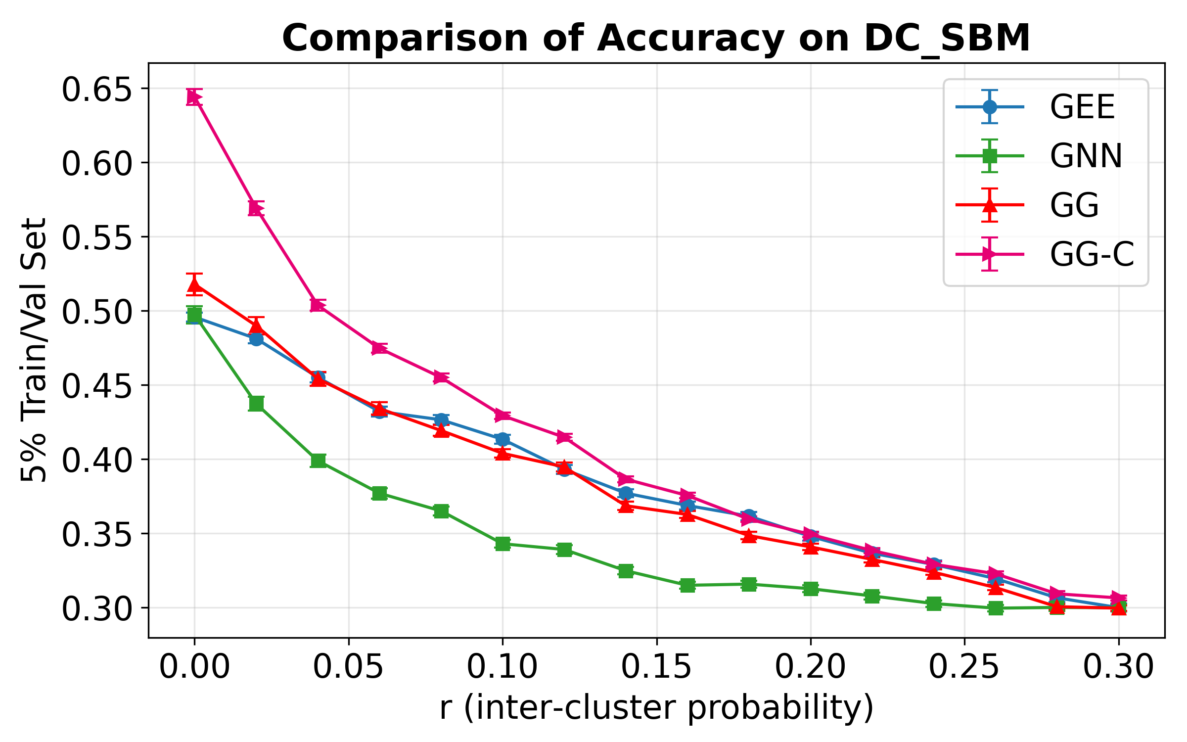
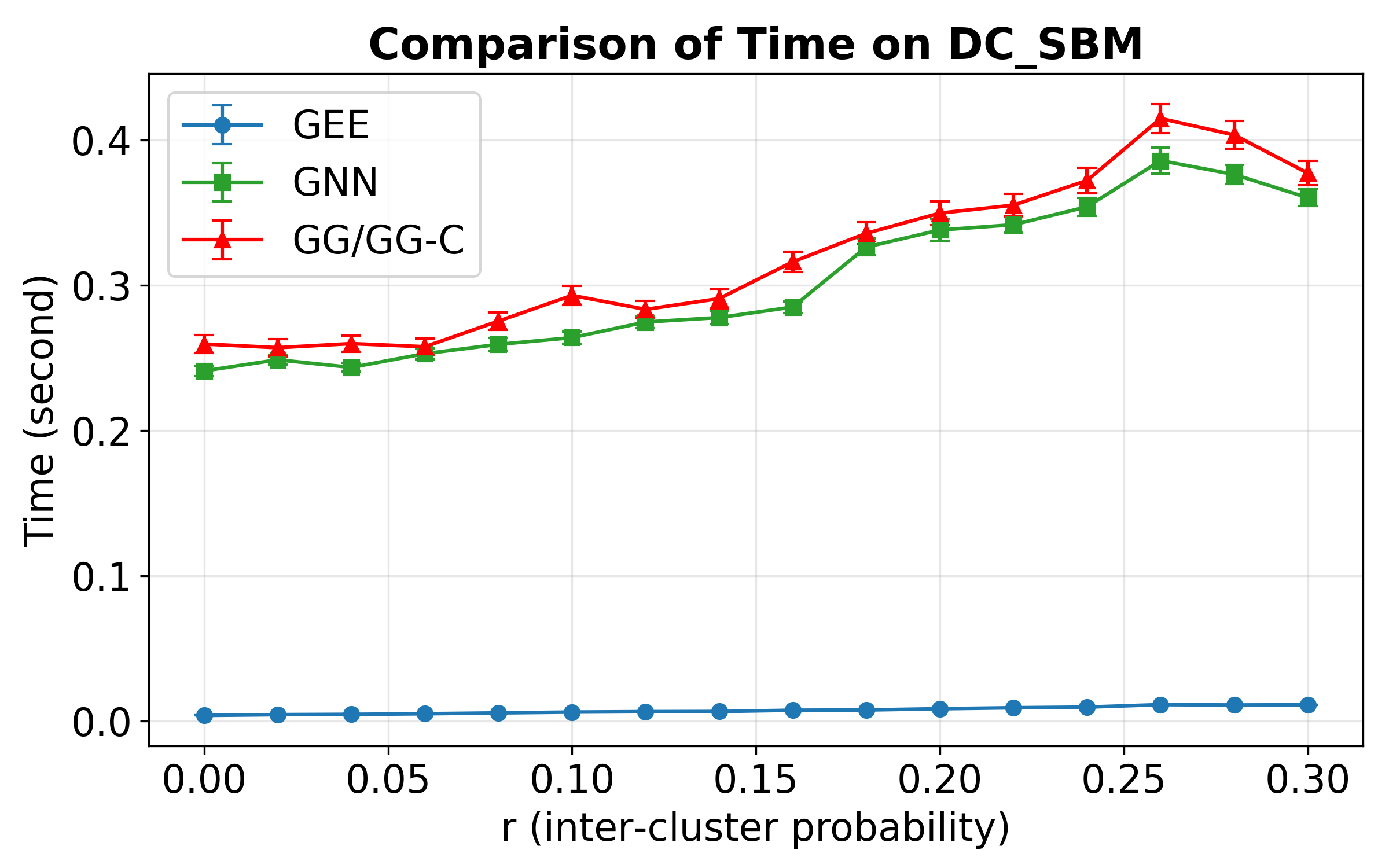
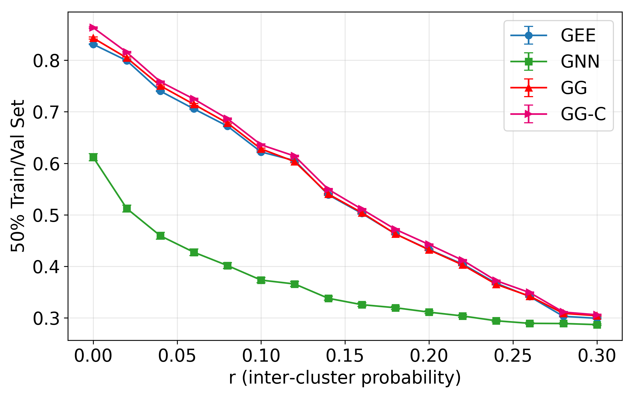
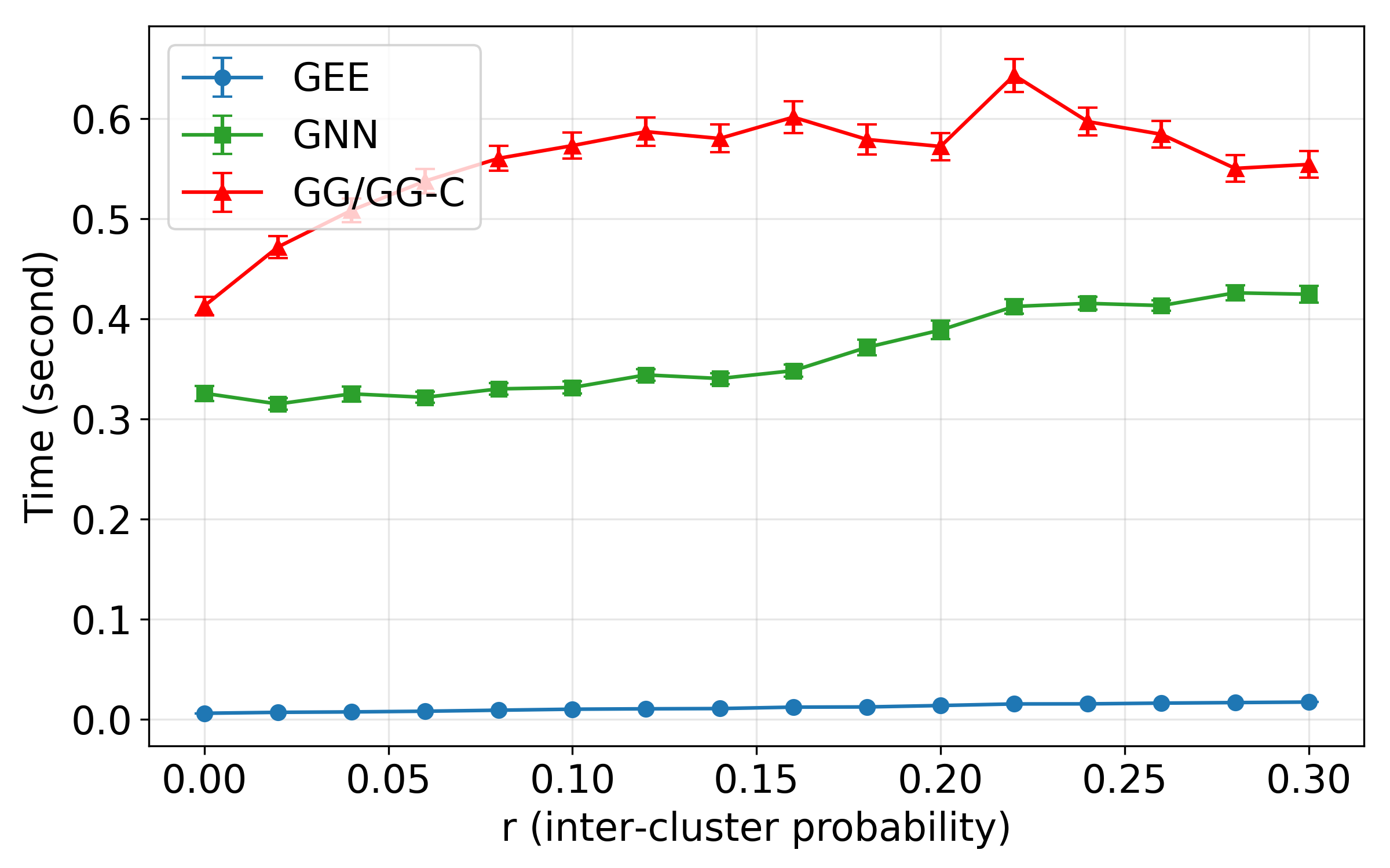
Figure 3: Classification performance comparison of GEE, GNN, GG and GG-C on DC-SBM graphs with 5% (top row) and 50% (bottom row) train/val set. This figure demonstrates the superiority of our GG and GG-C. They overcome the poor accuracy of the faster GNN (which is prone to local optima), while our concatenated variant, GG-C, also surpasses the classic GEE, particularly in the challenging low-label (5%) setting.

Each method is evaluated by the classification accuracy. For a given set of nodes $\mathcal{V}$, accuracy is defined as the fraction of correctly classified nodes. We denote this metric as $\text{Acc}(\mathcal{V})$ and formalize it as:

$$\text{Acc}(\mathcal{V})=\frac{1}{|\mathcal{V}|}\sum_{i\in\mathcal{V}}\mathbb{I}(\hat{Y}_{i}=Y_{i}),$$

where $\hat{Y}_{i}$ is the predicted label for node $i$ and $Y_{i}$ is its ground-truth label.

During training, we employ an early stopping strategy for the GNN-based methods by monitoring accuracy on a separate validation set, $\text{Acc}(\mathcal{V}_{\text{val}})$. The model parameters from the epoch that yields the highest validation accuracy are restored for the final evaluation on the test set, $\text{Acc}(\mathcal{V}_{\text{test}})$. To ensure a fair comparison, GEE is also evaluated under the same conditions, where the labels of nodes in the validation set are masked alongside the test set labels and are not used during its embedding generation process.

Regarding the running time of GG-C, it is reported jointly with GG in our figures and tables. This is because the additional computational cost of GG-C, which involves a simple feature concatenation and a non-intensive classifier like Linear Discriminant Analysis (LDA), is negligible compared to training process shared with GG. Therefore, for practical purposes, their running times are considered identical.

TABLE III: Classification accuracy and running time on real-world datasets of 5% train/val data. For accuracy, the best and second-best results are highlighted in bold and italic, respectively. For the GNN-based models (GNN, GG and GG-C), the fastest running time is also marked in bold. The running time of GEE is not highlighted and is excluded from direct comparison due to its non-iterative nature.

	ACM	BAT	DBLP	EAT	UAT	Wiki	Gene	IIP
Accuracy
GEE	0.469$\pm$0.002	0.412$\pm$0.006	0.316$\pm$0.001	0.364$\pm$0.005	0.415$\pm$0.005	0.244$\pm$0.004	0.575$\pm$0.004	0.410$\pm$0.014
GNN	0.427$\pm$0.004	0.294$\pm$0.005	0.297$\pm$0.002	0.321$\pm$0.005	0.358$\pm$0.005	0.224$\pm$0.003	0.525$\pm$0.006	0.515$\pm$0.008
GG	0.492$\pm$0.005	0.382$\pm$0.007	0.329$\pm$0.002	0.351$\pm$0.005	0.404$\pm$0.006	0.326$\pm$0.003	0.531$\pm$0.005	0.510$\pm$0.010
GG-C	0.534$\pm$0.003	0.425$\pm$0.008	0.336$\pm$0.003	0.370$\pm$0.005	0.435$\pm$0.004	0.304$\pm$0.003	0.549$\pm$0.003	0.444$\pm$0.010
Running time (s)
GEE	0.01$\pm$0.00	0.00$\pm$0.00	0.00$\pm$0.00	0.00$\pm$0.00	0.01$\pm$0.00	0.01$\pm$0.00	0.00$\pm$0.00	0.00$\pm$0.00
GNN	0.37$\pm$0.01	0.14$\pm$0.00	0.30$\pm$0.01	0.21$\pm$0.01	0.32$\pm$0.01	0.74$\pm$0.02	0.16$\pm$0.00	0.13$\pm$0.00
GG/GG-C	0.37$\pm$0.01	0.14$\pm$0.00	0.28$\pm$0.01	0.22$\pm$0.01	0.30$\pm$0.01	0.77$\pm$0.02	0.14$\pm$0.00	0.13$\pm$0.00

	LastFM	PolBlogs	TerroristRel	KarateClub	Chameleon	Cora	Citeseer
Accuracy
GEE	0.333$\pm$0.004	0.723$\pm$0.005	0.737$\pm$0.010	0.648$\pm$0.016	0.267$\pm$0.004	0.349$\pm$0.006	0.244$\pm$0.002
GNN	0.431$\pm$0.003	0.706$\pm$0.009	0.683$\pm$0.006	0.257$\pm$0.012	0.288$\pm$0.003	0.318$\pm$0.006	0.238$\pm$0.003
GG	0.536$\pm$0.003	0.729$\pm$0.014	0.718$\pm$0.011	0.663$\pm$0.019	0.270$\pm$0.004	0.393$\pm$0.005	0.280$\pm$0.003
GG-C	0.509$\pm$0.003	0.815$\pm$0.009	0.765$\pm$0.006	0.729$\pm$0.014	0.333$\pm$0.003	0.426$\pm$0.004	0.303$\pm$0.003
Running time (s)
GEE	0.01$\pm$0.00	0.01$\pm$0.00	0.00$\pm$0.00	0.00$\pm$0.00	0.01$\pm$0.00	0.00$\pm$0.00	0.00$\pm$0.00
GNN	1.58$\pm$0.04	0.34$\pm$0.01	0.26$\pm$0.01	0.13$\pm$0.00	0.57$\pm$0.01	0.38$\pm$0.01	0.36$\pm$0.01
GG/GG-C	2.18$\pm$0.05	0.30$\pm$0.01	0.25$\pm$0.01	0.13$\pm$0.00	0.56$\pm$0.02	0.39$\pm$0.02	0.38$\pm$0.01

TABLE IV: Classification accuracy and running time on real-world datasets of 50% train/val data. For accuracy, the best and second-best results are highlighted in bold and italic, respectively. For the GNN-based models (GNN, GG and GG-C), the fastest running time is also marked in bold. The running time of GEE is not highlighted and is excluded from direct comparison due to its non-iterative nature.

	ACM	BAT	DBLP	EAT	UAT	Wiki	Gene	Industry
Accuracy
GEE	0.749$\pm$0.002	0.350$\pm$0.008	0.538$\pm$0.001	0.314$\pm$0.008	0.497$\pm$0.003	0.592$\pm$0.001	0.762$\pm$0.002	0.601$\pm$0.005
GNN	0.544$\pm$0.008	0.370$\pm$0.007	0.379$\pm$0.005	0.357$\pm$0.005	0.385$\pm$0.006	0.406$\pm$0.006	0.606$\pm$0.009	0.511$\pm$0.006
GG	0.751$\pm$0.004	0.319$\pm$0.008	0.532$\pm$0.002	0.248$\pm$0.005	0.439$\pm$0.005	0.617$\pm$0.001	0.704$\pm$0.009	0.614$\pm$0.005
GG-C	0.759$\pm$0.002	0.394$\pm$0.007	0.536$\pm$0.002	0.385$\pm$0.007	0.472$\pm$0.004	0.612$\pm$0.001	0.744$\pm$0.003	0.624$\pm$0.005
Running time (s)
GEE	0.01$\pm$0.00	0.00$\pm$0.00	0.00$\pm$0.00	0.00$\pm$0.00	0.01$\pm$0.00	0.01$\pm$0.00	0.00$\pm$0.00	0.00$\pm$0.00
GNN	0.40$\pm$0.01	0.14$\pm$0.00	0.32$\pm$0.01	0.24$\pm$0.01	0.37$\pm$0.01	0.85$\pm$0.04	0.19$\pm$0.01	0.14$\pm$0.00
GG/GG-C	0.70$\pm$0.03	0.13$\pm$0.00	0.54$\pm$0.02	0.21$\pm$0.01	0.47$\pm$0.02	0.93$\pm$0.02	0.18$\pm$0.01	0.14$\pm$0.00

	LastFM	PolBlogs	TerroristRel	KarateClub	Chameleon	Cora	Citeseer
Accuracy
GEE	0.717$\pm$0.001	0.907$\pm$0.002	0.899$\pm$0.001	0.826$\pm$0.011	0.263$\pm$0.004	0.724$\pm$0.001	0.545$\pm$0.001
GNN	0.621$\pm$0.003	0.737$\pm$0.012	0.712$\pm$0.012	0.390$\pm$0.015	0.281$\pm$0.002	0.477$\pm$0.006	0.373$\pm$0.005
GG	0.773$\pm$0.001	0.869$\pm$0.011	0.865$\pm$0.010	0.803$\pm$0.014	0.320$\pm$0.004	0.739$\pm$0.002	0.577$\pm$0.002
GG-C	0.766$\pm$0.001	0.915$\pm$0.002	0.908$\pm$0.002	0.838$\pm$0.009	0.379$\pm$0.004	0.749$\pm$0.002	0.582$\pm$0.001
Running time (s)
GEE	0.02$\pm$0.00	0.01$\pm$0.00	0.01$\pm$0.00	0.00$\pm$0.00	0.02$\pm$0.00	0.00$\pm$0.00	0.00$\pm$0.00
GNN	1.58$\pm$0.04	0.43$\pm$0.01	0.29$\pm$0.01	0.12$\pm$0.00	0.62$\pm$0.03	0.46$\pm$0.02	0.44$\pm$0.01
GG/GG-C	2.80$\pm$0.08	0.48$\pm$0.03	0.36$\pm$0.02	0.12$\pm$0.00	1.05$\pm$0.05	0.78$\pm$0.03	0.74$\pm$0.02

VI-B Simulation

Here we present two most representative train/val set proportions on DC-SBM: 50% (data-rich) and 5% (data-scarce), in Figure 3. The complete results, including those for the 10% and 20% train/val set proportions on DC-SBM and all results for SBM, are provided in Appendix. The graph generation parameters for this classification task are identical to those used in the clustering evaluation, except that we perform 200 independent runs.

From the left two panels, it is evident that both GG and GG-C substantially outperform the vanilla GNN. A closer comparison with GEE sheds light on the underlying dynamics. When provided with sufficient training data (e.g., $50\%$ of nodes labeled), GEE performs remarkably well, aligning with its theoretical guarantees. In such cases, GG and GG-C achieve similar high accuracy, indicating that GEE alone is already near-optimal. However, as the proportion of training/validation data decreases (see Appendix for results under $10\%$ and $20\%$ training), GEE’s performance begins to degrade, though it still remains superior to the vanilla GNN.

In the semi-supervised regime, GG provides a meaningful refinement over GEE, but its standalone accuracy does not substantially surpass GEE’s until GG-C is introduced. This provides a key insight: GEE offers a strong initialization, GG contributes nontrivial refinement, and their concatenation, combined with an LDA classifier, produces a fused representation that effectively leverages both global structural information from GEE and localized refinements from the GNN. In this view, GG-C acts as a hybrid model where the GEE component also serves as a regularizer, mitigating over-reliance on potentially noisy GNN outputs and promoting more stable and accurate predictions.

From the right two panels, an interesting observation emerges: the vanilla GNN appears to converge slightly faster than the GG-based models. However, this should not be interpreted as better efficiency. Rather, it reflects premature convergence to a suboptimal local minimum, a common consequence of poor initialization, which may terminate early without achieving meaningful optimization. Importantly, the time difference between GG and vanilla GNN is marginal and negligible across all classification tasks.

VI-C Real data

For experiments on real-world datasets, we performed 100 independent runs for each data split to ensure statistical robustness. All publicly available datasets were included in our evaluation, with the exception of the Email dataset, which was excluded due to several classes containing fewer than three samples, violating our minimum class size requirement. Results for the 5% and 50% training/validation set proportions are presented in Table III and Table IV, respectively. Additional results for the 10% and 20% settings are provided in Appendix.

Both GG and GEE serve as strong baselines, and in most cases outperform the vanilla GNN. However, neither consistently dominates the other across all datasets. By contrast, the GG-C version, which fuses the embeddings from both GG and GEE, successfully captures complementary information from both global and local representations. As a result, it achieves superior performance across a diverse set of graph data. In nearly every case, GG-C either ranks as the top performer or closely follows the best-performing method in terms of classification accuracy.

VII Conclusion

In this work, we introduced the GEE-powered GNN (GG) method, grounded in the core insight that improved feature initialization can mitigate the well-known challenges associated with random initializations in graph Neural networks, such as slow convergence and convergence to suboptimal solutions. Through extensive experiments on both synthetic and real-world datasets, we demonstrated that GG consistently enhances performance across node-level tasks. For node clustering, the GEE-based warm-start enables GG to better explore the optimization landscape, leading to faster convergence and superior clustering quality. For node classification, where the loss function is task-specific and the optimization may trade off between global and local structure, our concatenated variant GG-C strikes an effective balance, retaining global information from GEE while benefiting from local refinement through GNN.

These findings point to a promising direction in GNN research: rather than focusing solely on deeper or more sophisticated neural architectures, substantial improvements can be achieved by designing more principled initialization strategies. Such strategies act as a form of implicit regularization, improving generalization and reducing the risk of overfitting, particularly in low-label or semi-supervised settings. Among many graph embedding algorithms, we chose GEE for its statistical properties and computational efficiency, providing a theoretical-sound node features with minimal overhead.

The broader implications of this work extend beyond graph learning. The idea of leveraging statistically informed, structure-aware initializations can be applied to a wide range of neural architectures. There are multiple avenues for future research, such as extensions to dynamic or temporal graphs where initialization may adapt to evolving structure, and generalization to non-graph domains such as recommendation systems or vision, where a combination of pretrained features and local refinement could be similarly beneficial.

Shiyu Chen received the B.E. degree in computer science from Sun Yat-sen University, Guangzhou, China, in 2024. He is currently pursuing the M.S. degree in data science at Johns Hopkins University. His research interests include graph neural networks, random graph models, and statistical learning on graphs.

Cencheng Shen received the BS degree in Quantitative Finance from National University of Singapore in 2010, and the PhD degree in Applied Mathematics and Statistics from Johns Hopkins University in 2015. He is an associate professor in the Department of Applied Economics and Statistics at University of Delaware. His research interests include graph embedding, dependence measures, and neural networks.

Youngser Park received the B.E. degree in electrical engineering from Inha University in Seoul, Korea in 1985, the M.S. and Ph.D. degrees in computer science from The George Washington University in 1991 and 2011 respectively. From 1998 to 2000 he worked at the Johns Hopkins Medical Institutes as a senior research engineer. From 2003 until 2011 he worked as a senior research analyst, and has been an associate research scientist since 2011 then research scientist since 2019 in the Center for Imaging Science at the Johns Hopkins University. At Johns Hopkins, he holds joint appointments in the The Institute for Computational Medicine and the Human Language Technology Center of Excellence. His current research interests are clustering algorithms, pattern classification, and data mining for high-dimensional and graph data.

Carey E. Priebe received the BS degree in mathematics from Purdue University in 1984, the MS degree in computer science from San Diego State University in 1988, and the PhD degree in information technology (computational statistics) from George Mason University in 1993. From 1985 to 1994 he worked as a mathematician and scientist in the US Navy research and development laboratory system. Since 1994 he has been a professor in the Department of Applied Mathematics and Statistics at Johns Hopkins University. His research interests include computational statistics, kernel and mixture estimates, statistical pattern recognition, model selection, and statistical inference for high-dimensional and graph data. He is a Senior Member of the IEEE, an Elected Member of the International Statistical Institute, a Fellow of the Institute of Mathematical Statistics, and a Fellow of the American Statistical Association.

APPENDIX

VIII Clustering Evaluation

This section provides supplementary results for our methods on graphs generated by Stochastic Block Model (SBM) [27]. The SBM can be understood as a simplified case of the DC-SBM (described in the main text) that does not account for degree heterogeneity. The probability of an edge between nodes $i$ and $j$ depends solely on their community assignments, with the adjacency matrix $A$ being generated as: $A(i,j)\sim\text{Bernoulli}(B(Y_{i},Y_{j}))$.

For this experiment, we generate graphs with $n=800$ nodes and $K=4$ imbalanced communities (1:2:3:4 ratio). We fix the intra-community link probability to $0.15$ and vary the inter-community link probability, $r$, from $0$ to $0.15$.

The results for clustering accuracy (ARI) and running time are presented in Figure 4. The trends are highly consistent with the DC-SBM experiments, confirming that GG is the best overall method. While GEE excels in low-noise settings ($r<0.06$), its performance sharply declines in more challenging scenarios. This dropoff is so significant that it even hinders GG’s performance, which underscores the need for a high-quality and stable initialization to achieve optimal results efficiently.

IX Classification Evaluation

IX-A Simulation

This subsection provides supplementary results for our simulation studies on classification task. To offer a more complete picture of model performance on DC-SBM under varying data scarcity, we present the results for training proportions of 10% and 20% in Figure 5.

Additionally, for the classification task on SBM graphs, we used the same graph generation parameters as in the clustering study but conducted 200 independent trials for each graph generated at every value of $r$ to ensure high statistical confidence. The results for SBM across all data-splitting ratios are presented in Figures 6.

IX-B Real Data

Table V summarizes the performance on real-world datasets with 10% and 20% of nodes used for training and validation. Across these settings, our GG-C consistently delivers the top performance, closely followed by our GG.

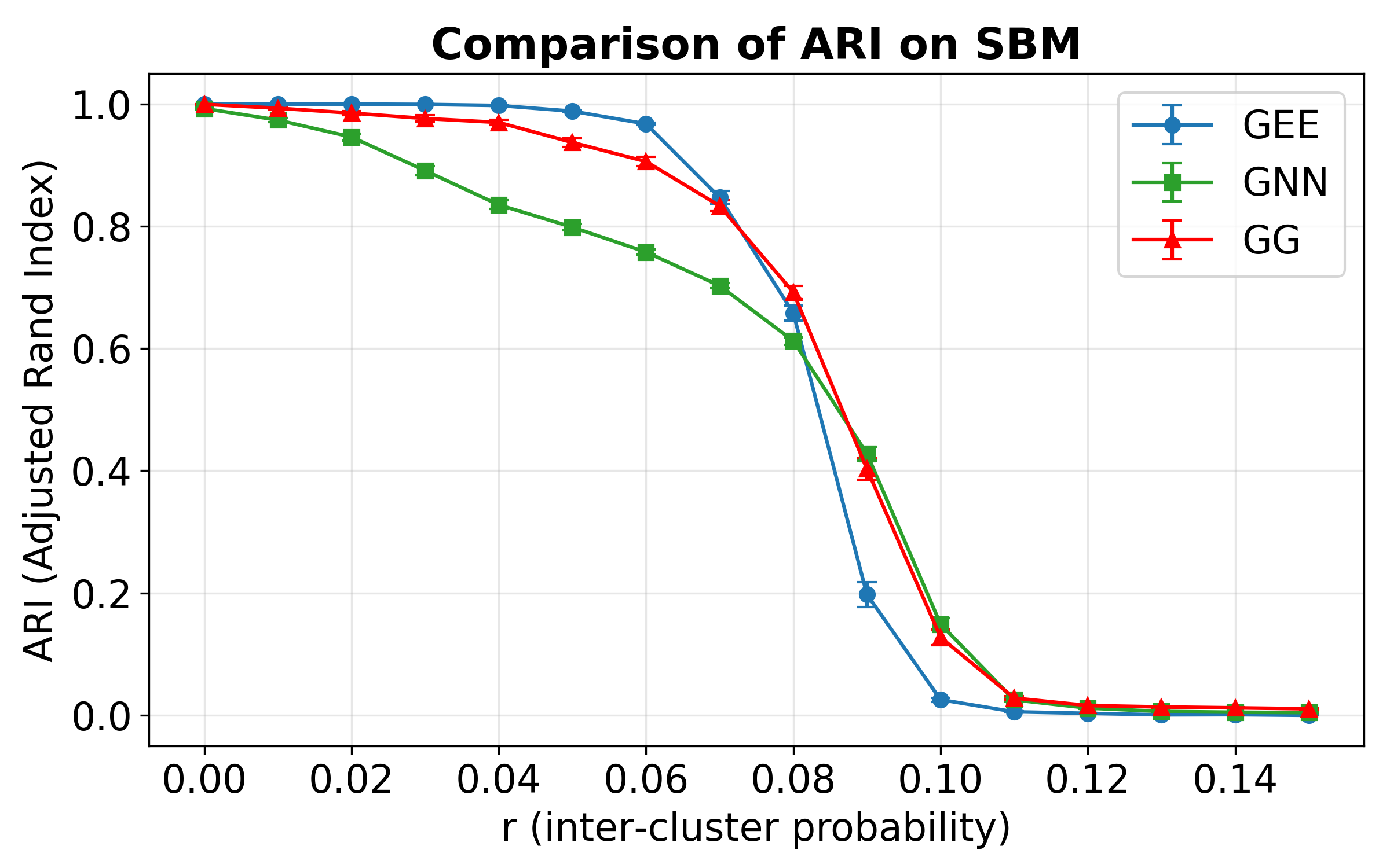
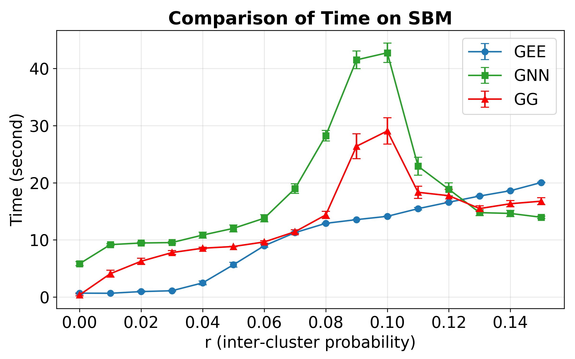
Figure 4: Clustering performance comparison of GEE, GNN and GG on SBM graphs. This figure shows our GG method significantly outperforms the vanilla GNN in both accuracy and speed. Crucially, it also surpasses the classic GEE on more challenging graphs ($r>0.08$), making it the most effective method overall.

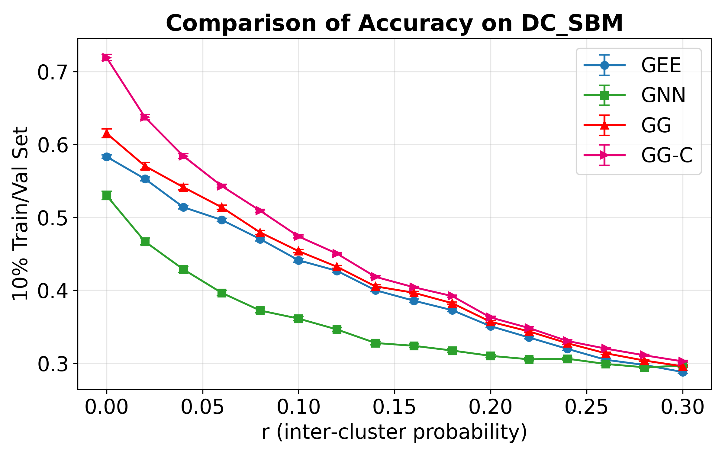
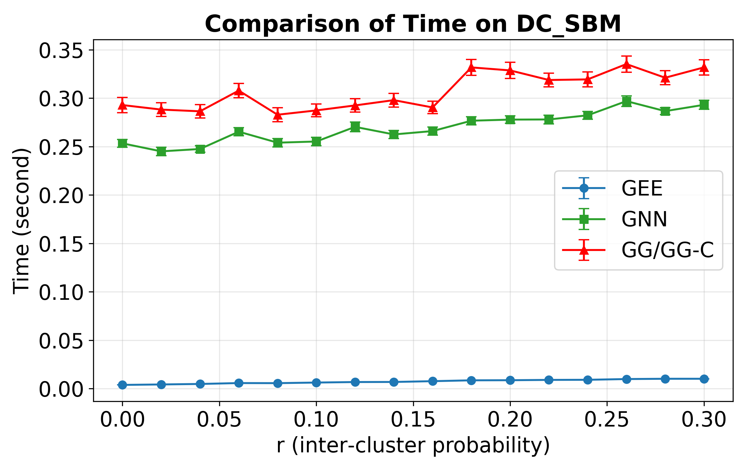
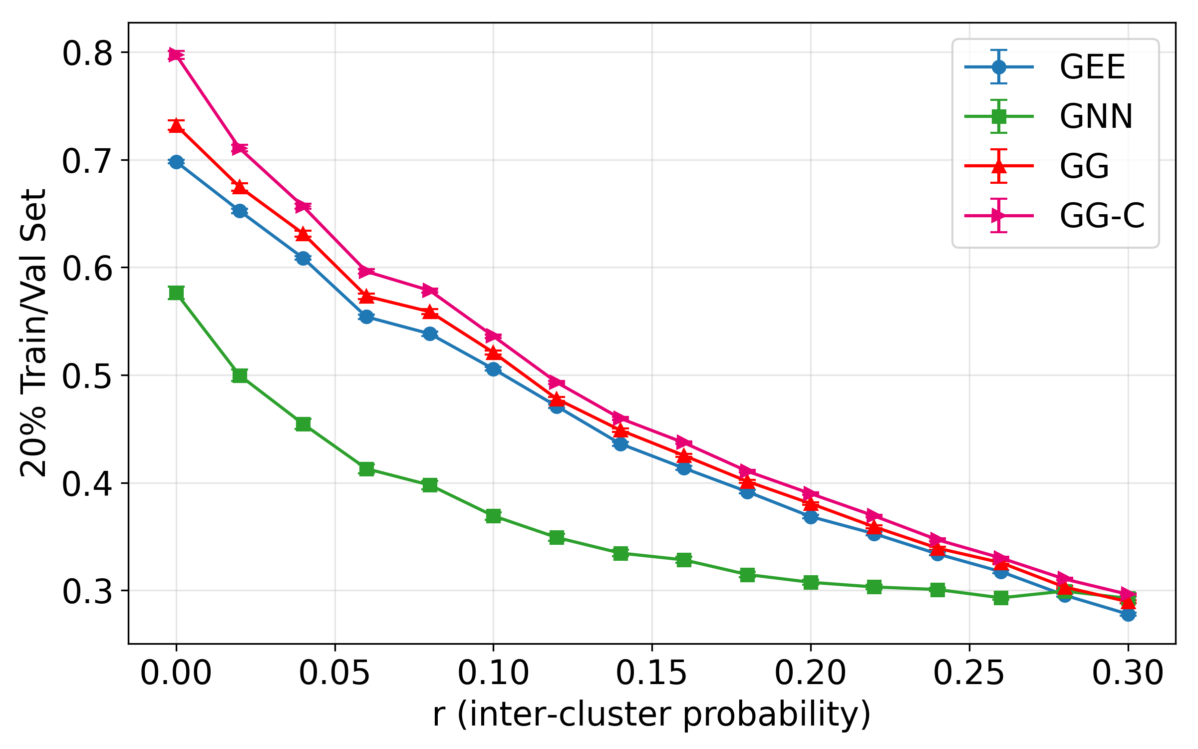
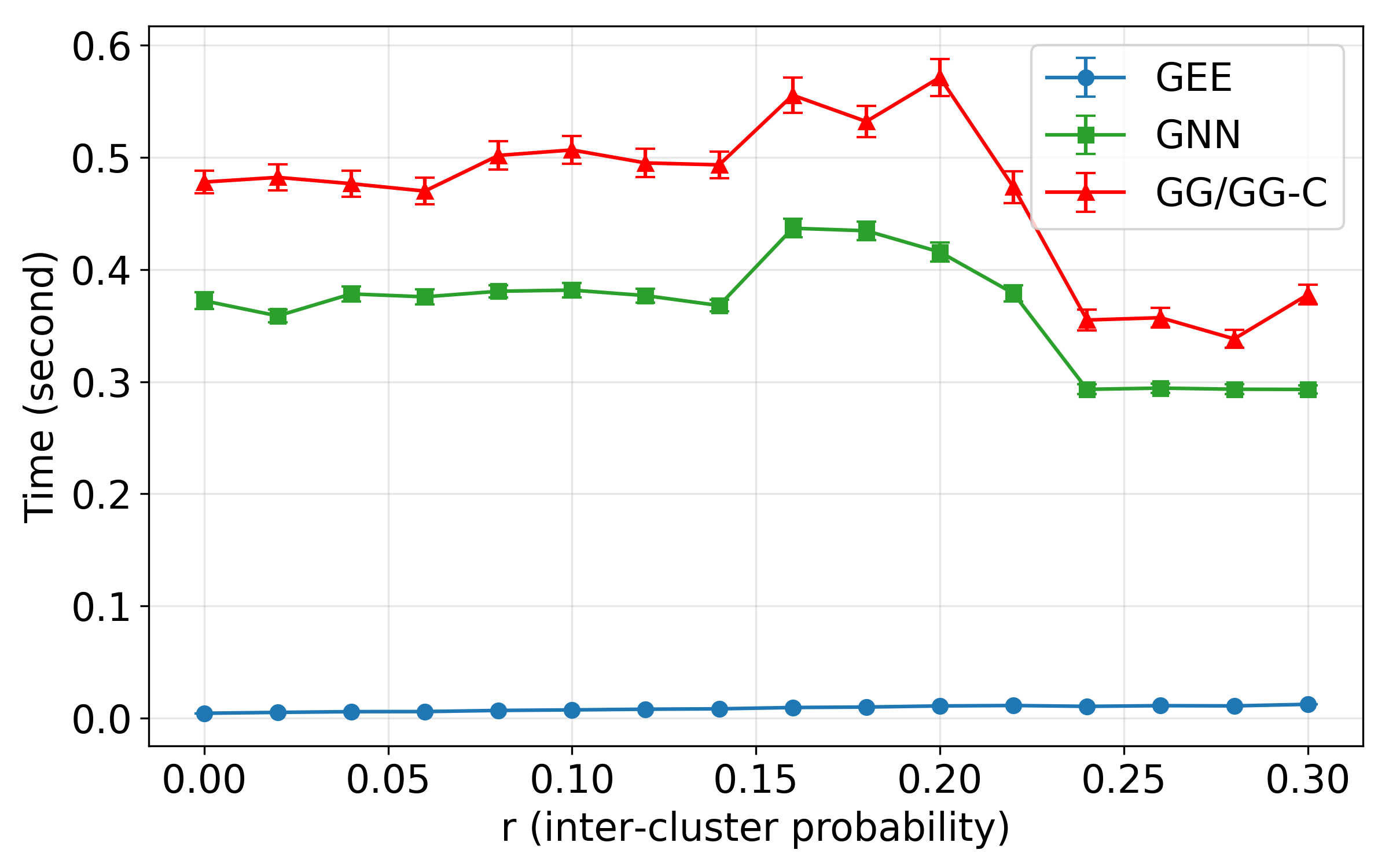
Figure 5: Classification performance comparison of GEE, GNN, GG and GG-C on DC-SBM graphs with 10% (top row) and 20% (bottom row) train/val set. The results show that GG and GG-C consistently deliver the best performance. They not only overcome the poor accuracy of the faster GNN, which is prone to local optima, but they also demonstrate a distinct advantage over GEE, especially as the amount of labeled data decreases.

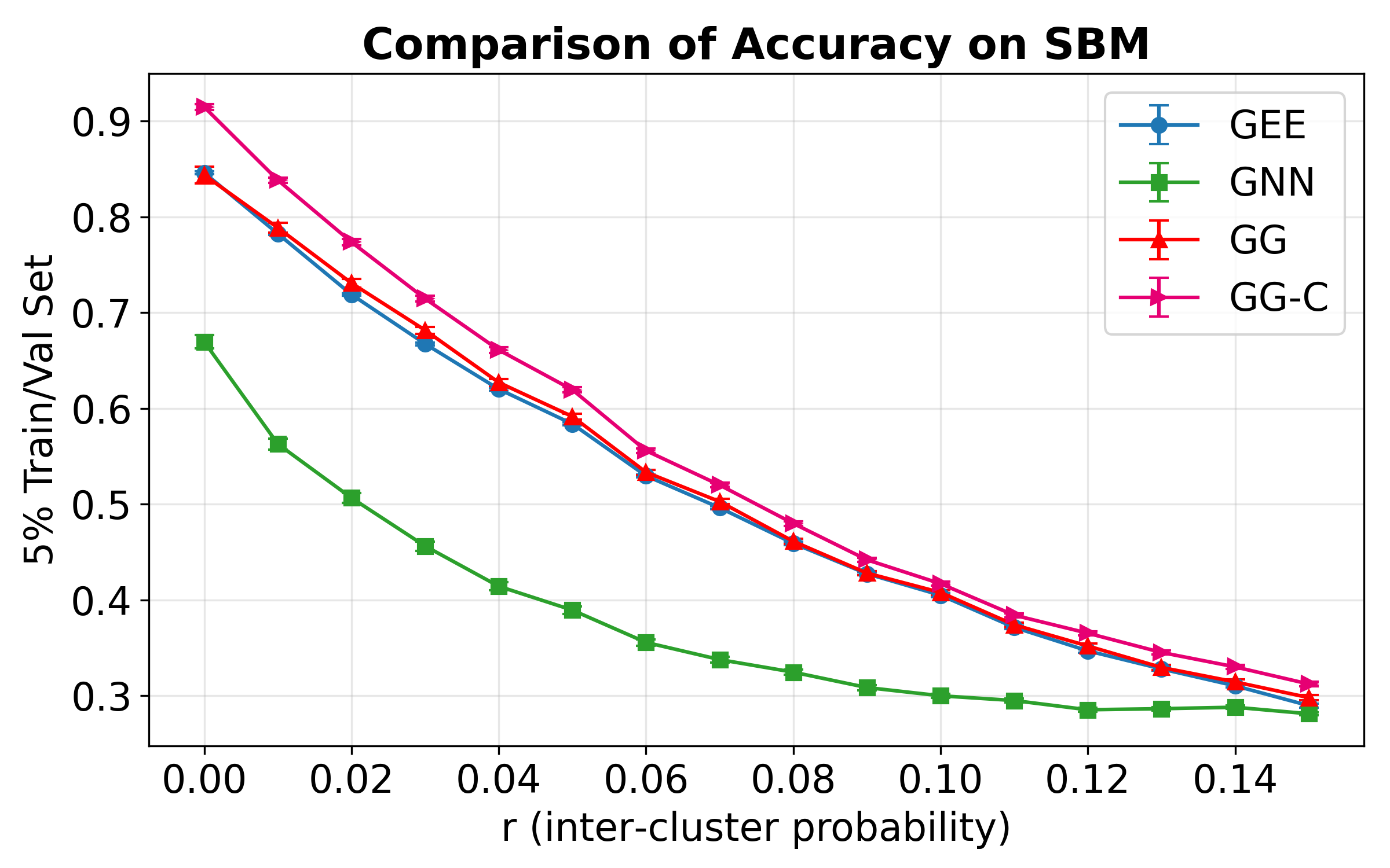
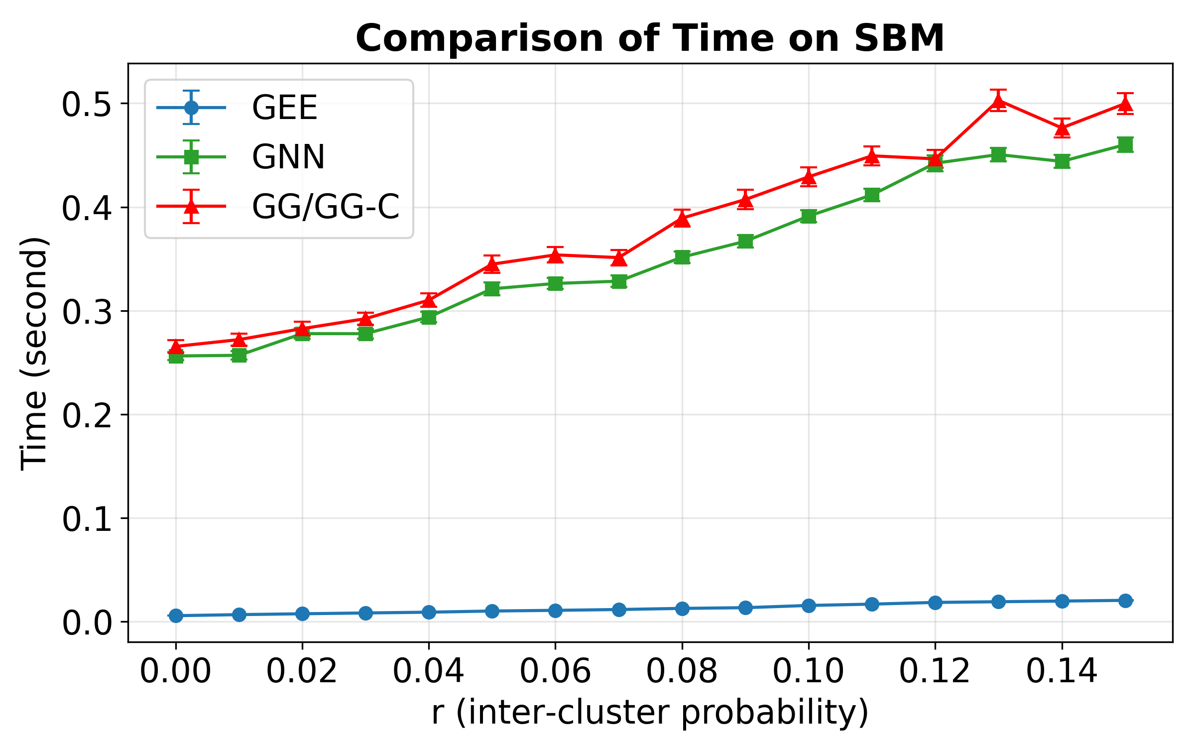
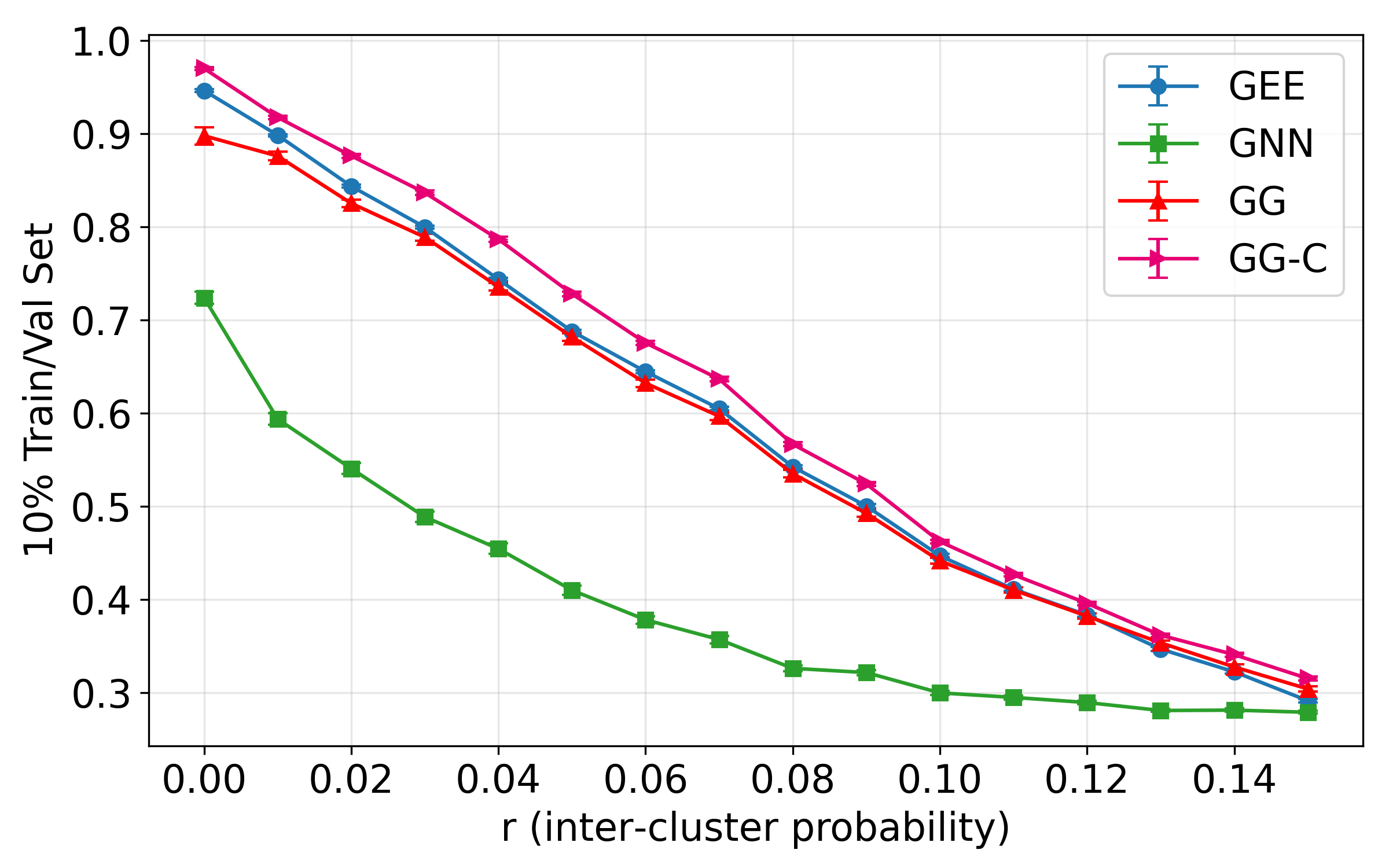
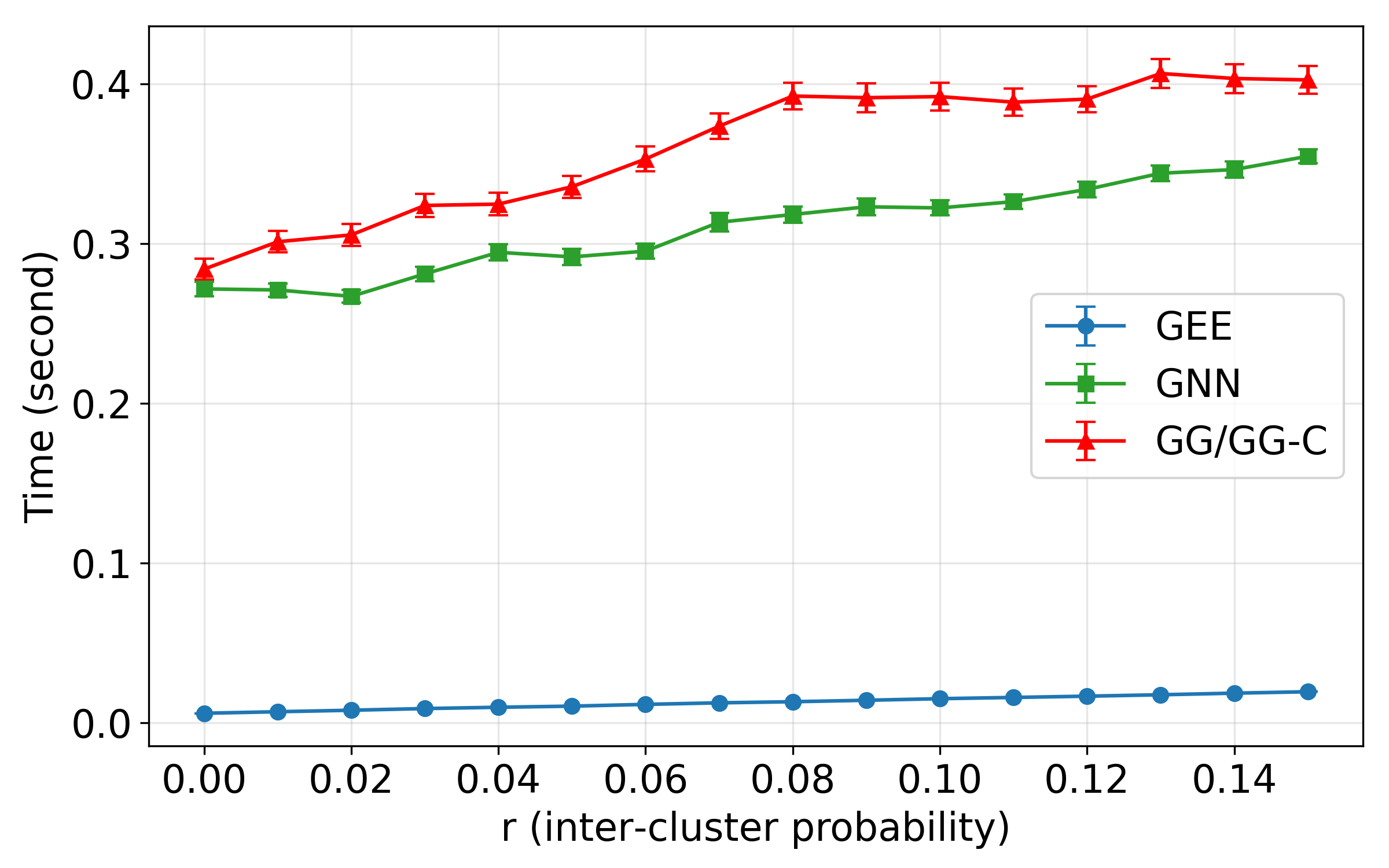
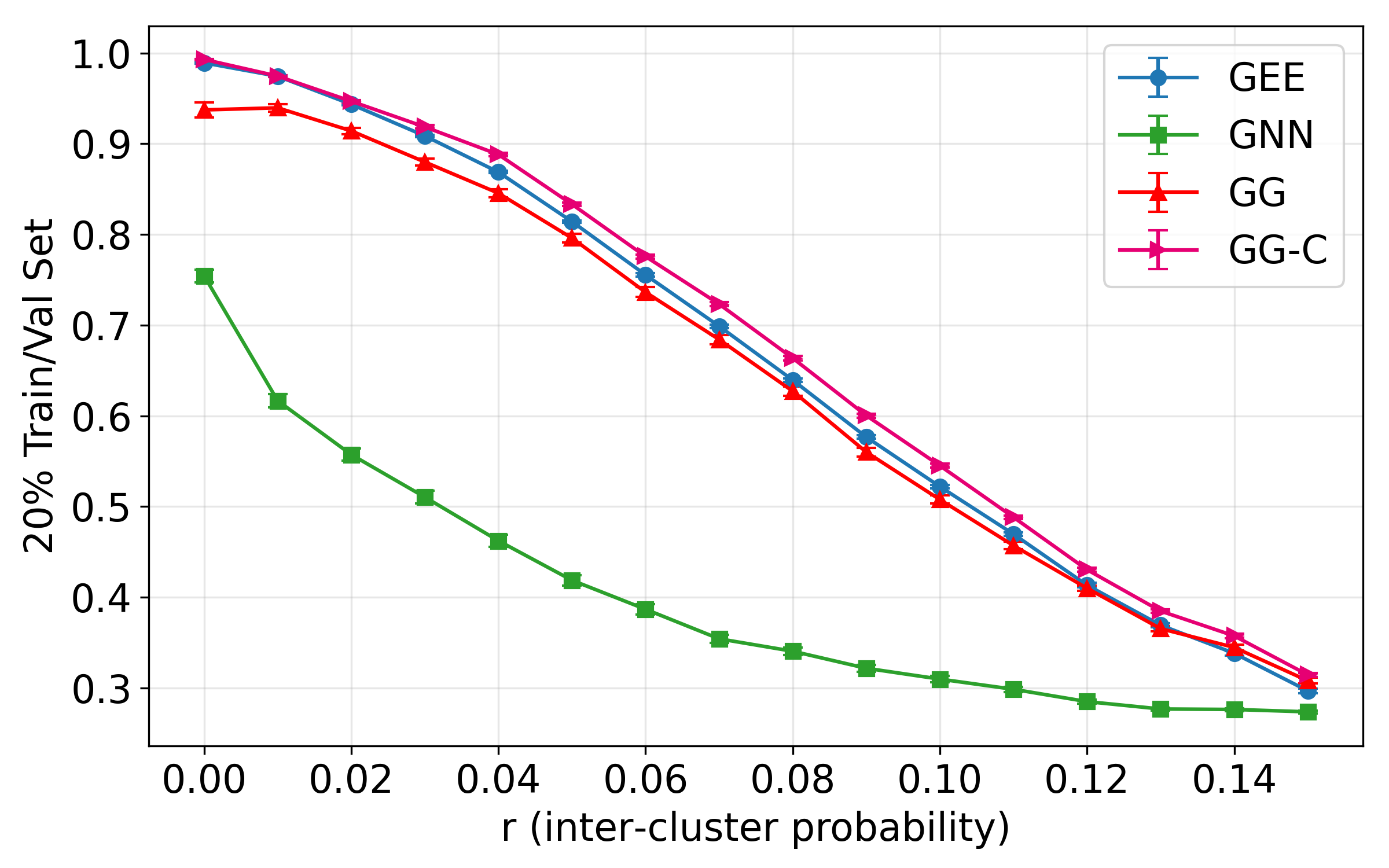
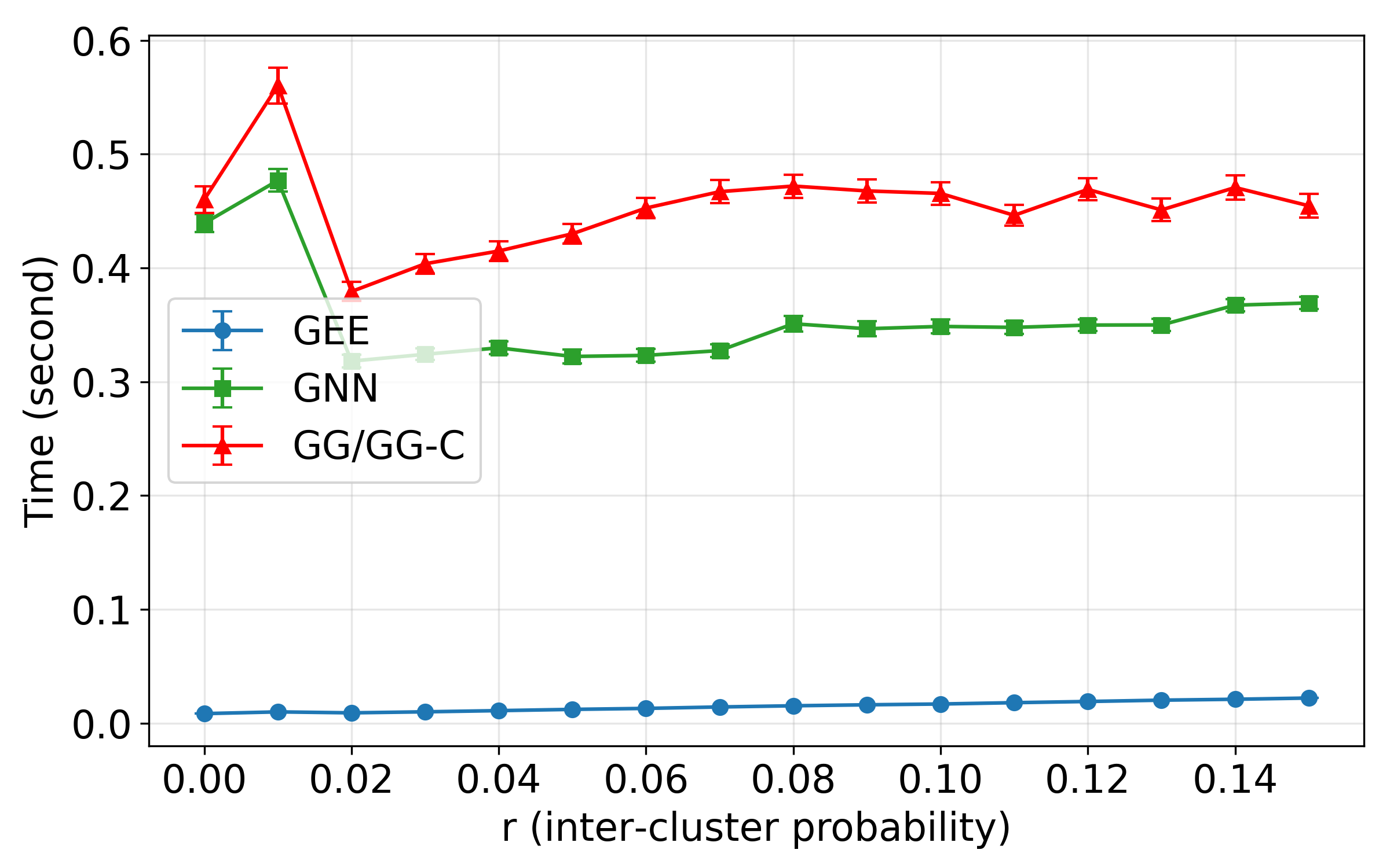
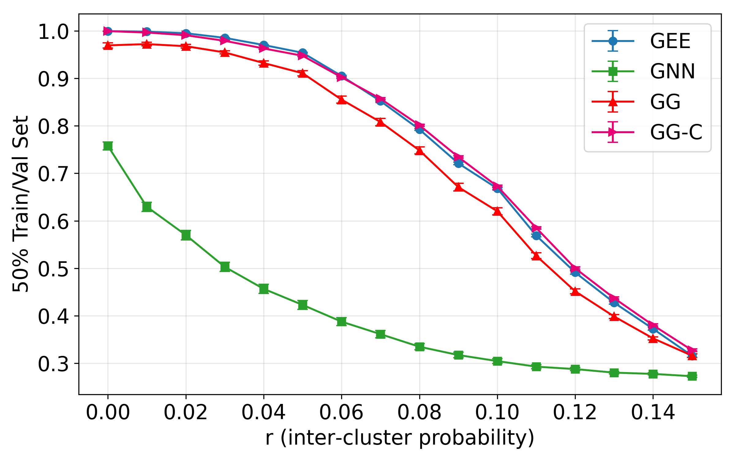
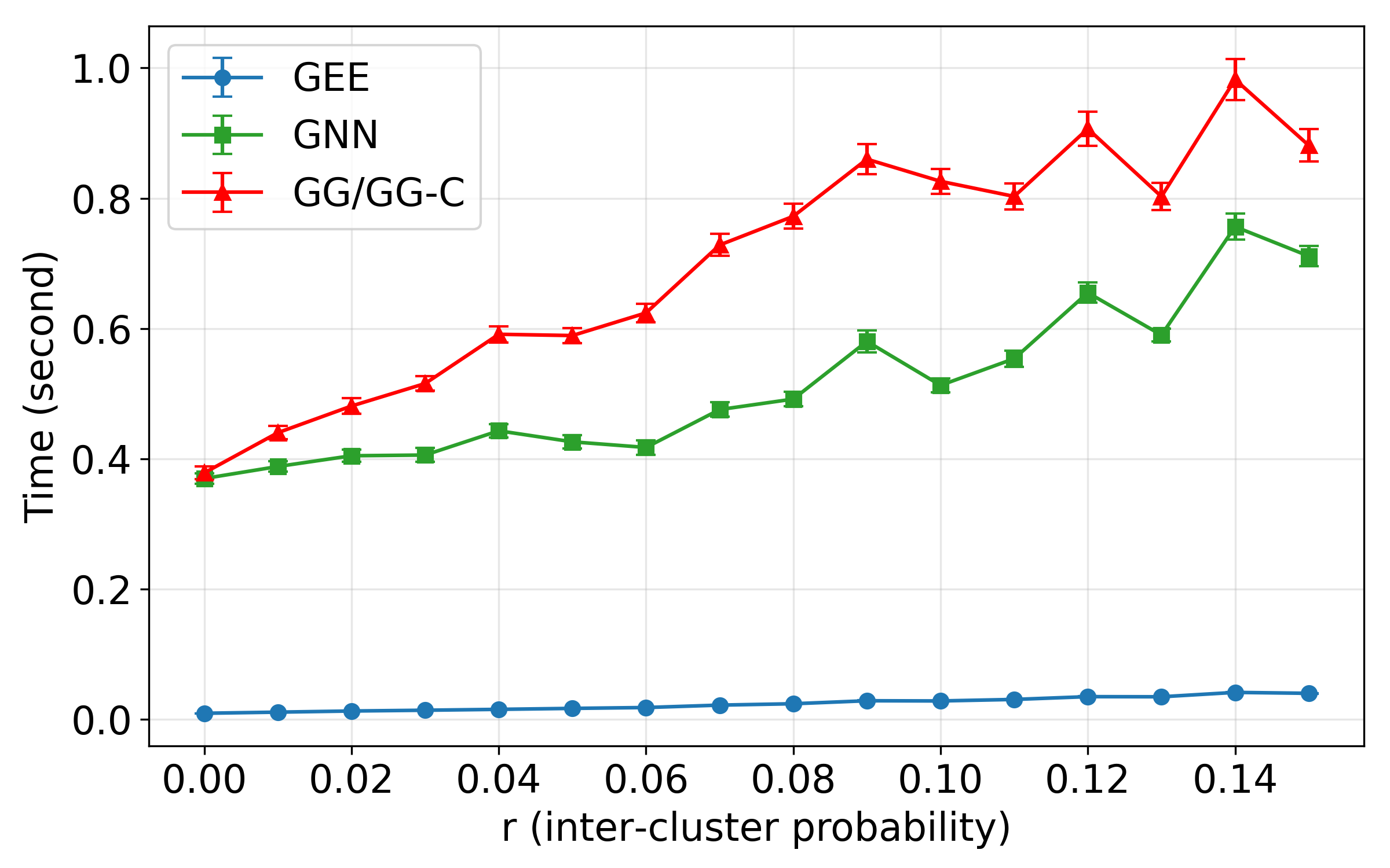
Figure 6: Classification performance comparison of GEE, GNN, GG, and GG-C on SBM graphs. Each row corresponds to a different proportion of nodes used for the train/val set, ranging from 5% (top row) to 50% (bottom row). This figure confirms the superiority of our GG and GG-C methods. They consistently outperform the fast-but-inaccurate GNN (prone to local optima), and the advantage of GG-C over GEE is most significant in low-label settings (e.g., 5% and 10%), showcasing their excellent data efficiency for semi-supervised learning.

TABLE V: Classification accuracy and running time on real-world datasets with 10% (top) and 20% (bottom) train/val data. For accuracy, the best and second-best results are highlighted in bold and italic, respectively. For the GNN-based models (GNN, GG and GG-C), the fastest running time is also marked in bold. The running time of GEE is not highlighted and is excluded from direct comparison due to its non-iterative nature.

(a) Results with 10% Train/Val Data
	ACM	BAT	DBLP	EAT	UAT	Wiki	Gene	IIP
Accuracy
GEE	0.546$\pm$0.002	0.424$\pm$0.006	0.353$\pm$0.001	0.380$\pm$0.006	0.473$\pm$0.003	0.353$\pm$0.003	0.618$\pm$0.003	0.509$\pm$0.010
GNN	0.464$\pm$0.005	0.304$\pm$0.005	0.309$\pm$0.003	0.333$\pm$0.005	0.377$\pm$0.004	0.283$\pm$0.003	0.544$\pm$0.006	0.524$\pm$0.006
GG	0.565$\pm$0.006	0.392$\pm$0.008	0.365$\pm$0.002	0.335$\pm$0.006	0.430$\pm$0.005	0.419$\pm$0.002	0.567$\pm$0.005	0.536$\pm$0.009
GG-C	0.603$\pm$0.002	0.427$\pm$0.007	0.376$\pm$0.003	0.380$\pm$0.005	0.467$\pm$0.003	0.411$\pm$0.002	0.594$\pm$0.003	0.527$\pm$0.007
Running time (s)
GEE	0.01$\pm$0.00	0.00$\pm$0.00	0.00$\pm$0.00	0.00$\pm$0.00	0.01$\pm$0.00	0.01$\pm$0.00	0.00$\pm$0.00	0.00$\pm$0.00
GNN	0.38$\pm$0.01	0.14$\pm$0.00	0.32$\pm$0.01	0.21$\pm$0.01	0.35$\pm$0.01	0.76$\pm$0.02	0.18$\pm$0.01	0.13$\pm$0.00
GG/GG-C	0.48$\pm$0.02	0.13$\pm$0.00	0.35$\pm$0.01	0.22$\pm$0.01	0.35$\pm$0.01	0.79$\pm$0.02	0.14$\pm$0.00	0.12$\pm$0.00

	LastFM	PolBlogs	TerroristRel	KarateClub	Chameleon	Cora	Citeseer
Accuracy
GEE	0.444$\pm$0.002	0.780$\pm$0.004	0.815$\pm$0.005	0.648$\pm$0.016	0.283$\pm$0.004	0.450$\pm$0.002	0.302$\pm$0.002
GNN	0.495$\pm$0.003	0.729$\pm$0.009	0.699$\pm$0.007	0.257$\pm$0.012	0.309$\pm$0.003	0.359$\pm$0.005	0.267$\pm$0.005
GG	0.601$\pm$0.002	0.770$\pm$0.013	0.797$\pm$0.009	0.663$\pm$0.019	0.283$\pm$0.004	0.478$\pm$0.005	0.344$\pm$0.003
GG-C	0.592$\pm$0.002	0.842$\pm$0.007	0.835$\pm$0.003	0.729$\pm$0.014	0.354$\pm$0.003	0.515$\pm$0.004	0.362$\pm$0.003
Running time (s)
GEE	0.02$\pm$0.00	0.01$\pm$0.00	0.00$\pm$0.00	0.00$\pm$0.00	0.01$\pm$0.00	0.00$\pm$0.00	0.00$\pm$0.00
GNN	1.87$\pm$0.05	0.36$\pm$0.01	0.27$\pm$0.01	0.13$\pm$0.00	0.63$\pm$0.02	0.40$\pm$0.01	0.36$\pm$0.01
GG/GG-C	2.33$\pm$0.05	0.33$\pm$0.01	0.30$\pm$0.01	0.12$\pm$0.00	0.64$\pm$0.03	0.51$\pm$0.02	0.46$\pm$0.02

(b) Results with 20% Train/Val Data
	ACM	BAT	DBLP	EAT	UAT	Wiki	Gene	IIP
Accuracy
GEE	0.634$\pm$0.001	0.410$\pm$0.008	0.413$\pm$0.001	0.354$\pm$0.007	0.507$\pm$0.002	0.460$\pm$0.002	0.665$\pm$0.003	0.558$\pm$0.006
GNN	0.500$\pm$0.006	0.331$\pm$0.005	0.333$\pm$0.003	0.341$\pm$0.004	0.389$\pm$0.005	0.351$\pm$0.003	0.564$\pm$0.007	0.505$\pm$0.005
GG	0.646$\pm$0.005	0.375$\pm$0.007	0.419$\pm$0.003	0.299$\pm$0.005	0.448$\pm$0.005	0.512$\pm$0.002	0.616$\pm$0.007	0.560$\pm$0.009
GG-C	0.670$\pm$0.002	0.415$\pm$0.008	0.429$\pm$0.003	0.368$\pm$0.006	0.484$\pm$0.003	0.504$\pm$0.002	0.647$\pm$0.003	0.574$\pm$0.006
Running time (s)
GEE	0.01$\pm$0.00	0.00$\pm$0.00	0.00$\pm$0.00	0.00$\pm$0.00	0.01$\pm$0.00	0.01$\pm$0.00	0.00$\pm$0.00	0.00$\pm$0.00
GNN	0.39$\pm$0.01	0.13$\pm$0.00	0.32$\pm$0.01	0.23$\pm$0.01	0.40$\pm$0.01	0.85$\pm$0.03	0.20$\pm$0.01	0.13$\pm$0.00
GG/GG-C	0.59$\pm$0.03	0.13$\pm$0.00	0.43$\pm$0.02	0.22$\pm$0.01	0.44$\pm$0.02	0.91$\pm$0.02	0.16$\pm$0.01	0.13$\pm$0.00

	LastFM	PolBlogs	TerroristRel	KarateClub	Chameleon	Cora	Citeseer
Accuracy
GEE	0.560$\pm$0.001	0.842$\pm$0.003	0.865$\pm$0.002	0.648$\pm$0.016	0.279$\pm$0.004	0.554$\pm$0.002	0.385$\pm$0.002
GNN	0.556$\pm$0.002	0.746$\pm$0.012	0.710$\pm$0.009	0.257$\pm$0.012	0.313$\pm$0.003	0.408$\pm$0.005	0.308$\pm$0.003
GG	0.672$\pm$0.002	0.816$\pm$0.012	0.829$\pm$0.013	0.663$\pm$0.019	0.293$\pm$0.004	0.584$\pm$0.004	0.430$\pm$0.002
GG-C	0.666$\pm$0.002	0.874$\pm$0.005	0.873$\pm$0.002	0.729$\pm$0.014	0.373$\pm$0.003	0.609$\pm$0.003	0.439$\pm$0.002
Running time (s)
GEE	0.02$\pm$0.00	0.01$\pm$0.00	0.00$\pm$0.00	0.00$\pm$0.00	0.02$\pm$0.00	0.00$\pm$0.00	0.00$\pm$0.00
GNN	1.77$\pm$0.06	0.41$\pm$0.01	0.29$\pm$0.01	0.12$\pm$0.00	0.64$\pm$0.02	0.42$\pm$0.01	0.39$\pm$0.01
GG/GG-C	2.48$\pm$0.06	0.39$\pm$0.02	0.30$\pm$0.01	0.12$\pm$0.00	0.70$\pm$0.03	0.66$\pm$0.02	0.65$\pm$0.02

References

- [1] T. N. Kipf and M. Welling, “Semi-supervised classification with graph convolutional networks,” arXiv preprint arXiv:1609.02907, 2016.
- [2] ——, “Variational graph auto-encoders,” arXiv preprint arXiv:1611.07308, 2016.
- [3] W. L. Hamilton, R. Ying, and J. Leskovec, “Inductive representation learning on large graphs,” in Proceedings of the 31st International Conference on Neural Information Processing Systems, ser. NIPS ’17, vol. 30, 2017, pp. 1025–1035.
- [4] P. Veličković, G. Cucurull, A. Casanova, A. Romero, P. Liò, and Y. Bengio, “Graph attention networks,” in Proceedings of ICLR, 2018.
- [5] M. Schlichtkrull, T. N. Kipf, P. Bloem, R. Van Den Berg, I. Titov, and M. Welling, “Modeling relational data with graph convolutional networks,” in The semantic web: 15th international conference, ESWC 2018, Heraklion, Crete, Greece, June 3–7, 2018, proceedings 15. Springer, 2018, pp. 593–607.
- [6] M. Zhang and Y. Chen, “Link prediction based on graph neural networks,” in Proceedings of the 32nd International Conference on Neural Information Processing Systems, ser. NeurIPS ’18, vol. 31, 2018, pp. 5161–5170.
- [7] M. Zhang, P. Li, Y. Xia, K. Wang, and L. Jin, “Labeling trick: A theory of using graph neural networks for multi-node representation learning,” Advances in Neural Information Processing Systems, vol. 34, pp. 9061–9073, 2021.
- [8] A. Tsitsulin, J. Palowitch, B. Perozzi, and E. Müller, “Graph clustering with graph neural networks,” Journal of Machine Learning Research, vol. 24, no. 127, pp. 1–21, 2023.
- [9] H. Cai, V. W. Zheng, and K. C.-C. Chang, “A comprehensive survey of graph embedding: Problems, techniques, and applications,” IEEE transactions on knowledge and data engineering, vol. 30, no. 9, pp. 1616–1637, 2018.
- [10] Z. Wu, S. Pan, F. Chen, G. Long, C. Zhang, and S. Y. Philip, “A comprehensive survey on graph neural networks,” IEEE transactions on neural networks and learning systems, vol. 32, no. 1, pp. 4–24, 2020.
- [11] Z. Zhang, P. Cui, and W. Zhu, “Deep learning on graphs: A survey,” IEEE Transactions on Knowledge and Data Engineering, vol. 34, no. 1, pp. 249–270, 2022.
- [12] C. E. Priebe, C. Shen, N. Huang, and T. Chen, “A simple spectral failure mode for graph convolutional networks,” IEEE Transactions on Pattern Analysis and Machine Intelligence, vol. 44, no. 11, pp. 8689–8693, 2022.
- [13] C. Shen, Q. Wang, and C. E. Priebe, “One-hot graph encoder embedding,” IEEE Transactions on Pattern Analysis and Machine Intelligence, vol. 45, no. 6, pp. 7933–7938, 2022.
- [14] C. Shen, J. Larson, H. Trinh, and C. E. Priebe, “Refined graph encoder embedding via self-training and latent community recovery,” Social Network Analysis and Mining, vol. 15, p. 14, 2025.
- [15] C. Shen, Y. Dong, C. E. Priebe, J. Larson, H. Trinh, and Y. Park, “Principal graph encoder embedding and principal community detection,” IEEE Transactions on Network Science and Engineering, 2025.
- [16] C. Shen, J. Larson, H. Trinh, X. Qin, Y. Park, and C. E. Priebe, “Discovering communication pattern shifts in large-scale labeled networks using encoder embedding and vertex dynamics,” IEEE Transactions on Network Science and Engineering, vol. 11, no. 2, pp. 2100–2109, 2024.
- [17] C. Shen, C. E. Priebe, J. Larson, and H. Trinh, “Synergistic graph fusion via encoder embedding,” Information Sciences, vol. 678, p. 120912, 2024.
- [18] C. Shen, “Encoder embedding for general graph and node classification,” Applied Network Science, vol. 9, p. 66, 2024.
- [19] G. Li, M. Muller, A. Thabet, and B. Ghanem, “Deepgcns: Can gcns go as deep as cnns?” in Proceedings of the IEEE/CVF international conference on computer vision, 2019, pp. 9266–9275.
- [20] M. E. Newman and M. Girvan, “Finding and evaluating community structure in networks,” Physical review E, vol. 69, no. 2, p. 026113, 2004.
- [21] U. Brandes, D. Delling, M. Gaertler, R. Gorke, M. Hoefer, Z. Nikoloski, and D. Wagner, “On modularity clustering,” IEEE transactions on knowledge and data engineering, vol. 20, no. 2, pp. 172–188, 2008.
- [22] B. H. Good, Y.-A. De Montjoye, and A. Clauset, “Performance of modularity maximization in practical contexts,” Physical Review E—Statistical, Nonlinear, and Soft Matter Physics, vol. 81, no. 4, p. 046106, 2010.
- [23] S. Fortunato, “Community detection in graphs,” Physics reports, vol. 486, no. 3-5, pp. 75–174, 2010.
- [24] V. Traag, L. Waltman, and N. Van Eck, “From louvain to leiden: guaranteeing well-connected communities. sci. rep. 9, 5233,” 2019.
- [25] X. Zhang, H. Liu, Q. Li, and X.-M. Wu, “Attributed graph clustering via adaptive graph convolution,” arXiv preprint arXiv:1906.01210, 2019.
- [26] D. Bo, X. Wang, C. Shi, M. Zhu, E. Lu, and P. Cui, “Structural deep clustering network,” in Proceedings of the web conference 2020, 2020, pp. 1400–1410.
- [27] P. W. Holland, K. B. Laskey, and S. Leinhardt, “Stochastic blockmodels: First steps,” Social networks, vol. 5, no. 2, pp. 109–137, 1983.
- [28] Y. Zhao, E. Levina, and J. Zhu, “Consistency of community detection in networks under degree-corrected stochastic block models,” Annals of Statistics, vol. 40, no. 4, pp. 2266–2292, 2012.
- [29] Y. Liu, J. Xia, S. Zhou, X. Yang, K. Liang, C. Fan, Y. Zhuang, S. Z. Li, X. Liu, and K. He, “A survey of deep graph clustering: Taxonomy, challenge, application, and open resource,” arXiv preprint arXiv:2211.12875, 2022.
- [30] S. Wang, J. Yang, J. Yao, Y. Bai, and W. Zhu, “An overview of advanced deep graph node clustering,” IEEE Transactions on Computational Social Systems, vol. 11, no. 1, pp. 1302–1314, 2024.