Implicit representations of codimension-2 submanifolds and their prequantum structure

Abstract

This paper explores the geometry of the space of codimension-2 submanifolds. We implicitly represent these submanifolds by a class of complex-valued functions. This reveals a prequantum bundle structure over the space of submanifolds, equipped with the well-known Marsden–Weinstein symplectic structure. This bundle allows a new physical interpretation of the Marsden–Weinstein structure as the curvature of a connection form, which measures the average of volumes swept by the deformation of the $\SS^{1}$-family of hypersurfaces, defined as the phases of a complex function implicitly representing a submanifold.

Keywords. Symplectic structure, space of submanifolds, prequantum bundle

2020 Mathematics Subject Classification. 53D05, 58D10, 58A25, 58B25

1 Introduction

We explore the geometry of the space of codimension-2 submanifolds, with a particular focus on their implicit representations and a prequantumm structure on the space of these implicit representations.

Codimension-1 submanifolds—such as curves on a surface and surfaces in a three dimensional space—can be implicitly represented using a level set function. This representation naturally extends to multi-codimensional submanifolds using multiple level set functions. Specifically, when the codimension is 2, submanifolds—such as curves in a three dimensional space and surfaces in a four dimensional space—can be expressed as the zero sets of complex-valued functions. Such implicit representations via complex functions are useful for studying the geometry and dynamics of submanifolds. For example, the authors of this article recently leveraged the infinite redundancy in the implicit representation of space curves to numerically simulate curve dynamics arising in fluid dynamics and differential geometry [IWC22]. Implicit representations using complex-valued functions also appear in earlier and recent literature, where they describe the dynamics of space curves, such as curve-shortening flow [RMXO01] and quantum vortex filaments governed by the Gross-Pitaevskii equation [OTH02, VKPS16, JS18].

The codimension-2 case is also significant in the study of Hamiltonian dynamical systems of shapes. The space of codimension-2 unparametrized embeddings (or immersions) into an ambient manifold equipped with a volume form is known to be an infinite-dimensional symplectic manifold (or an orbifold, for immersions), endowed with the so-called Marsden–Weinstein (MW) symplectic structure [MW83, Khe12]. This structure is considered canonical as it formally corresponds to the Kirillov-Kostant-Souriau form when submanifolds are viewed as linear functionals on the Lie algebra of divergence-free vector fields on the ambient manifold [MW83, Theorem 4.2] [AK98, Chapter VI, Proposition 3.6]. The MW structure plays a crucial role in the study of dynamical systems, as it gives rise to many physically motivated equations, including those governing fluid dynamics and elastica [HV03, Khe12, CKPP20].

In this article, we investigate the space of codimension-2 submanifolds implicitly represented by the zero sets of complex functions and study its geometric structures related to the MW structure. Let $M$ be an oriented manifold equipped with a volume form and let $\mathcal{O}$ be the space of codimension-2 submanifolds in $M$, represented by embeddings modulo reparametrization. We call $\mathcal{O}$ the explicit shape space. The implicit representation of each element in $\mathcal{O}$ is not unique, as multiple complex-valued functions can share the same zero set. This non-uniqueness makes the implicit shape space $\mathcal{F}_{\mathcal{O}}$ a fiber bundle over the explicit shape space $\mathcal{O}$. Each element $\psi\in\mathcal{F}_{\mathcal{O}}$ is a complex-valued function over $M$, while each point $\gamma\in\mathcal{O}$ is a codimension-2 submanifold in $M$. The projection from $\mathcal{F}_{\mathcal{O}}$ to $\mathcal{O}$ is to extract the zero set.

This bundle has a natural geometric interpretation. Each complex function $\psi\in\mathcal{F}_{\mathcal{O}}$ representing a codimension-2 submanifold $\gamma\in\mathcal{O}$ carries additional information in the form of its complex phase. The level sets of this phase function constitute a $\SS^{1}$-family of hypersurfaces in $M$, that are bordered by $\gamma$. Any motion of this configuration induces the average volume swept out by these phase hypersurfaces. In each fiber, we define two hypersurface configurations as equivalent ($\sim$) if they can be continuously deformed into each other while keeping their boundaries fixed and maintaining zero net volume change throughout the motion. The space of equivalence classes is denoted by $\mathcal{P}\coloneqq\mathcal{F}_{\mathcal{O}}/\sim$, which is still a fiber bundle over $\mathcal{O}$. We call $\mathcal{P}$ the volume class for the implicit shape space.

It turns out that the volume class $\mathcal{P}$ over $\mathcal{O}$ is a prequantum bundle, where each fiber consists of multiple copies of a circle, reflecting the first integral de Rham cohomology $H^{1}_{dR}(M,\mathbb{Z})$. The connection form $\Theta_{\mathcal{P}}$ on this bundle is defined such that the horizontal lift of any path in $\mathcal{O}$ corresponds to a motion of phase hypersurfaces that sweep out zero net volume along the path. With this setup, we have the following theorem.

Theorem 1.1 (Theorem 6.6).

The fibration $\Pi_{\mathcal{P}}\colon(\mathcal{P},\Theta_{\mathcal{P}})\to(\mathcal{O},\omega)$ is a prequantum $G$-bundle where $\omega$ is the MW symplectic form and the structure group is $G=\SS^{1}\times H^{1}_{dR}(M,\mathbb{Z})$.

In other words, the curvature of the connection $\Theta_{\mathcal{P}}$ agrees with the MW symplectic form. As a consequence, this prequantum bundle allows the following geometric interpretation of the MW form:

Corollary 1.2 (Section 6).

Consider a closed path $\partial\Sigma$ in $\mathcal{O}$ that bounds a 2-dimensional disk $\Sigma$, representing a cyclic motion of a codimension-2 submanifold $\gamma_{t}\subset M$ for $0\leq t\leq 1$, with $\gamma_{0}=\gamma_{1}$. Let $[\psi_{t}]_{\mathcal{P}}$ be a horizontal lift over $\gamma_{t}$ and $\phi_{t}\coloneqq\psi_{t}/|\psi_{t}|\colon M\setminus\psi^{-1}_{t}(0)\to\SS^{1}$ be the phase map of a representative $\psi_{t}\in[\psi_{t}]_{\mathcal{P}}$. Then $\gamma_{t}$ bounds a family of hypersurfaces $\{\sigma_{t}^{s}\}_{s\in\SS^{1}}$, defined by $\sigma_{t}^{s}=\phi_{t}^{-1}(s)$. Assume that the average volume swept out by $\sigma_{t}^{s}$ remains zero at each $t$, i.e.,

$$\frac{1}{2\pi}\int_{\SS^{1}}\int_{\sigma_{t}^{s}}\iota_{\partial_{t}{\sigma}_{t}^{s}}\mu\ ds=0,$$ (1.1)

where $\mu$ is the volume form on $M$.

Then, the volume enclosed between $\sigma_{0}^{s}$ and $\sigma_{1}^{s}$, averaged over $s\in\SS^{1}$, equals to $\iint_{\Sigma}\omega$, where $\omega$ is the MW form on $\mathcal{O}$.

In the limiting case of Section 1, where the phase of $\psi_{t}$ becomes constant except a $2\pi$ jump at on a single hypersurface $\sigma_{t}$ bounding $\gamma_{t}$, the result simplifies to the following corollary. This version has no explicit reference to the complex function $\psi_{t}$.

Corollary 1.3 (Section 6).

Let $\Sigma$ be a disc and $\{\gamma_{t}\}_{t\in[0,1]}$ be a path in $\mathcal{O}$ as in Section 1. Suppose that each $\gamma_{t}$ bounds a single hypersurface, i.e., $\gamma_{t}=\partial\sigma_{t}$, and that the volume swept out by $\sigma_{t}$ remains zero at each $t$. Then, the volume enclosed between $\sigma_{0}$ and $\sigma_{1}$ agrees with $\iint_{\Sigma}\omega$.

1.1 Related work

We briefly comment the previous work on Liouville forms and prequantum bundles over the codimension-2 shape space $\mathcal{O}$ equipped with the MW form, which are particularly relevant to this article.

Liouville forms for the explicit and the implicit settings

Recent works [Tab17, PCK⁺19] point out the existence of a Liouville form for the MW form (i.e., a 1-form $\eta$ such that $\omega=d\eta$) on the space of space curves. As an additional contribution to our main result, we extend this finding to the space of arbitrary oriented and closed codimension-2 submanifolds in an ambient manifold equipped with an exact volume form. The proof for the case of space curves presented in [Tab17] relies on an explicit parameterization of the curve, and therefore does not readily generalize to higher dimensional settings. We provide a parametrization-free proof using geometric measure theory.

Furthermore, we observe that the Liouville form introduced by [Tab17] for the MW form and our generalized ones on the explicit shape space are invariant only under a finite-dimensional subgroup of the volume-preserving diffeomorphisms of the ambient space. In contrast, the connection form $\Theta_{\mathcal{P}}$ we define, which serves as a Liouville form via the fibration $\Pi_{\mathcal{P}}$ (i.e., $\Pi_{\mathcal{P}}^{*}\omega=d\Theta_{\mathcal{P}}$), remains invariant under the full group of volume-preserving diffeomorphisms of the ambient space (Section 7.1.2).

Prequantum bundles over the codimension-2 shape spaces

There are other prequantum bundles over $(\mathcal{O},\omega)$. In [HV03], Haller and Vizman constructed a prequentum circle bundle by covering $\mathcal{O}$ with a collection of open sets $\{U_{i}\}_{i}$ and gluing the sets $\{\SS^{1}\times U_{i}\}_{i}$ using carefully chosen transition functions that ensure a prequantum bundle structure. Another approach, utilizing differential characters, was introduced in [DJNV20]. Presently we are not aware of any explicit relationships between their proposed prequantum bundles and ours.

However, we emphasize that, unlike these previously established prequantum bundle structures, our framework is inherently local. Specifically, we focus on submanifolds that are exact in homology, meaning they must bound codimension-1 domains. Consequently, the existence of our prequantum bundle is restricted to such exact submanifolds as we explain in Section 4.1.

Future work

The codimension-2 shape space admits not only the MW structure but also other symplectic structures, as recently shown in [BIM24]. In this article, we focus specifically on the MW structure. Extending our framework to a wider class of symplectic structures is an interesting direction for future work.

Secondly, we restrict our attention to the space of embeddings modulo reparametrization, meaning that self-intersecting shapes are outside the scope of this study, even though the MW form is defined on the space of immersions. On the other hand, the tools we employ from geometric measure theory, such as currents, are capable of handling such singularities. In the future, we aim to extend our framework to accommodate topological changes and reconnection events in shapes.

1.2 Organization of the paper

In Section 2, we review currents from geometric measure theory and introduce a diffeomorphism action on currents. This allows us to treat shapes in a parameterization-free manner in both explicit and implicit settings, and to rigorously handle the superposition of infinitely many hypersurfaces given as the phase level sets of implicit representations.

In Section 3, we review the MW symplectic structure on the explicit shape space $\mathcal{O}$ of codimension-2 submanifolds. We do so in terms of diffeomorphism actions on currents, highlighting that the deformation of a shape can be seen as the transport of a current along a vector field. Along the way, we extend the previous result on the existence of a Liouville form, which was known only for space curves (i.e., embeddings of a circle into $\mathbb{R}^{3}$), to a more general setting of embeddings of an oriented, closed manifold $S$ into a manifold $M$ equipped with an exact volume form.

In Section 4, we define implicit representations of codimension-2 submanifolds. We then study the geometry of the space of these implicit representations $\mathcal{F}_{\mathcal{O}}$ as a fiber bundle over $\mathcal{O}$.

In Section 5, we define a 1-form $\Theta$ on $\mathcal{F}_{\mathcal{O}}$ and show that it defines a Liouville form for the MW form $\omega\in\Omega^{2}(\mathcal{O})$ in the prequantum sense, i.e., $\Pi^{*}\omega=d\Theta$ via the fibration $\Pi\colon\mathcal{F}_{\mathcal{O}}\to\mathcal{O}$. Our proof, using geometric measure theory, offers a physical interpretation of $\Theta$ in terms of the swept volumes of phase hypersurfaces.

In Section 6, we define the volume class $\mathcal{P}$ as explained above. We show that $\Theta$ factored onto $\mathcal{P}$ becomes a connection form $\Theta_{\mathcal{P}}$ forming a prequantum $G$-bundle $\Pi_{\mathcal{P}}\colon(\mathcal{P},\Theta_{\mathcal{P}})\to(\mathcal{O},\omega)$ with the structure group $G=\SS^{1}\times H^{1}_{dR}(M,\mathbb{Z})$.

In Section 7, we study additional structures that implicit representations and prequantum structures reveal, such as horizontal Hamiltonian vector fields on $\mathcal{P}$ with respect to the connection $\Theta_{\mathcal{P}}$, and a degenerate formal Kähler structure on $\mathcal{F}_{\mathcal{O}}$.

Acknowledgement

We thank Chris Wojtan for his continuous support to the project through a number of discussions. We also thank Ioana Ciuclea, Bas Janssens, and Cornelia Vizman for discussions on prequantum bundles over nonlinear Grassmannians. The second author warmly acknowledges the hospitality of the University of California, San Diego, where part of this research was carried out during his visit.

This project was funded in part by the European Research Council (ERC Consolidator Grant 101045083 CoDiNA) and the National Science Foundation CAREER Award 2239062. Some figures in the article were generated by the software Houdini and its education license was provided by SideFX.

2 Preliminary: Diffeomorphism action on currents

We briefly review the notion of currents from geometric measure theory as a preliminary and define a diffeomorphism action on them. For readers interested in the general theory of currents, we refer to the literature [Fed14, dR84, Mor08]. Currents are a natural language for our implicit description of shapes embedded in an ambient manifold as they allow us to treat differential forms, submanifolds, and their generalizations in a unified manner. Using currents, we will describe relations between quantities defined on an ambient manifold and a submanifold (possibly with a boundary). This includes, for example, the flux of a vector field through a surface, and a superposition of the fluxes through infinitely many surfaces.

Let $M$ be an oriented $m$-dimensional manifold and $\Omega^{k}_{c}(M)$ be compactly supported differential $k$-forms. We say $k$-currents $\mathcal{D}_{k}(M)$, also denoted by $\Omega^{k}_{c}(M)^{*}$, are linear functionals on $\Omega_{c}^{k}(M)$ that are continuous in the sense of distributions. For details, see [CSdR12, Alb06] for example.

We note that $\Omega^{m-k}(M)\subset\mathcal{D}_{k}(M)$ via

$$\langle h,\alpha\rangle\coloneqq\int_{M}h\wedge\alpha,\quad h\in\Omega^{m-k}(M),\alpha\in\Omega_{c}^{k}(M).$$ (2.1)

The space of differential forms $\Omega^{m-k}(M)$ is strictly smaller than the space of current $\mathcal{D}_{k}(M)$, but $\mathcal{D}_{k}(M)$ is attained as the closure of $\Omega^{m-k}(M)$ with respect to the locally convex topology. Keeping this in mind, we will formally write $\int_{M}h\wedge\alpha$ also for $h$ in $\mathcal{D}_{k}(M)$ but not in $\Omega^{m-k}(M)$ as if $h$ was a $m-k$ form.

For $h\in\mathcal{D}_{k}(M)$, we define the boundary operator $\partial_{k}\colon\mathcal{D}_{k}(M)\to\mathcal{D}_{k-1}(M)$ by

$$\langle\partial_{k}h,\alpha\rangle\coloneqq\langle h,d_{k-1}\alpha\rangle,\quad\forall\alpha\in\Omega_{c}^{k}(M)$$ (2.2)

using the exterior derivative $d_{k-1}\colon\Omega^{k-1}(M)\to\Omega^{k}(M)$. Unless necessary, we will simply write $\partial$ for $\partial_{k}$ and $d$ for $d_{k}$. Notice that $\partial$ works for $h\in\Omega^{m-k}(M)\subset\mathcal{D}_{k}(M)$ as the exterior derivative $d$ up-to sign change with $\operatorname{sgn}=(-1)^{m-k+1}$,

We say that the current homology, which is the dual of de-Rham cohomology, is defined by

$$H^{CR}_{k}(M)\coloneqq Z^{CR}_{k}(M)/B^{CR}_{k}(M)$$ (2.3)

where $Z^{CR}_{k}(M)=\operatorname{ker}\partial_{k}$ and $B^{CR}_{k}(M)=\operatorname{im}\partial_{k+1}$.

2.1 de Rham-Dirac currents

We call a special class of currents de Rham-Dirac currents (or simply de Rham currents). These currents extend the Dirac measures for points (codimension-$m$ geometry) to other codimensions. For a $k$-dimensional submanifold $\Sigma$ of $M$ possibly with a boundary, we define a $k$-de Rham current $\delta_{\Sigma}\in\mathcal{D}_{k}(M)$ by

$$\langle\delta_{\Sigma},\alpha\rangle=\int_{\Sigma}\alpha,\quad\alpha\in\Omega^{k}(M).$$ (2.4)

We denote the collection of de Rham-$k$ current by $\mathcal{D}^{dR}_{k}(M)$.

The boundary operators $\partial$ for the de Rham currents and for submanifolds commute with the mapping of submanifolds to currents i.e., $\partial\delta_{\Sigma}=\delta_{\partial\Sigma}$ as

$$\langle\partial\delta_{\Sigma},\alpha\rangle=\int_{\Sigma}d\alpha=\int_{\partial\Sigma}\alpha=\langle\delta_{\partial\Sigma},\alpha\rangle,\quad\forall\alpha\in\Omega^{k}(M).$$ (2.5)

We will also formally write this as

$$\int_{M}\delta_{\partial\Sigma}\wedge\alpha=\int_{M}\delta_{\Sigma}\wedge d\alpha$$ (2.6)

with the mind of (2.1).

Remark 2.1.

de Rham currents can be defined from rectifiable sets on $M$, which form a much broader class containining submanifolds and singular chains of $M$ [Mor08]. In this article, we focus on the ones induced from submanifolds as it suffices for our purpose.

2.2 Orbits under diffeomorphism groups

In this article, we represent unparametrized shapes by currents and describe the deformation of shapes in terms of diffeomorphism actions. To do so, we define the action of diffeomorphism groups on currents and the Lie derivative as its infinitesimal generator.

Let us denote by $\operatorname{Diff}(M)$ the space of diffeomorphisms over $M$. For each $f\in\operatorname{Diff}(M)$, we define the action $f_{*}\colon D_{k}(M)\to D_{k}(M)$ by pushforward as the adjoint of pullback $f^{*}\colon\Omega^{k}(M)\to\Omega^{k}(M)$,

$$\langle f_{*}h,\alpha\rangle\coloneqq\langle h,f^{*}\alpha\rangle,\quad h\in\mathcal{D}_{k}(M),\alpha\in\Omega^{k}(M).$$ (2.7)

For $h\in\Omega^{m-k}(M)\subset\mathcal{D}_{k}(M)$, the pushforward action $f_{*}$ on $h$ as a current agrees with the pullback action ${f^{-1}}^{*}$ on $h$ as a differential form. For a de-Rham current $\delta_{\Sigma}\in\mathcal{D}_{k}^{dR}(M)$, we have $f_{*}\delta_{\Sigma}=\delta_{f\circ\Sigma}$. Note also that $f_{*}$ and $\partial$ commute similarly to the commutativity between $d$ and $f^{*}$ for differential forms.

On an orbit $\mathcal{O}$ under the $\operatorname{Diff}(M)$-action by pushforward, the tangent space is

$$T_{h}\mathcal{O}(M)=\{-\mathcal{L}_{v}h\mid v\in\operatorname{diff}(M)\}$$ (2.8)

where $\operatorname{diff}(M)$ is the Lie algebra of $\operatorname{Diff}(M)$, which is the space of smooth vector fields on $M$, and we say that Lie derivative $\mathcal{L}_{v}\colon\mathcal{D}(M)\to\mathcal{D}(M)$ for currents is the skew-adjoint of the Lie derivative for differential forms,

$$\langle-\mathcal{L}_{v}h,\alpha\rangle\coloneqq\langle h,\mathcal{L}_{v}\alpha\rangle,\quad\alpha\in\Omega^{k}(M).$$ (2.9)

The minus sign of $-\mathcal{L}_{v}h$ in (2.8) expresses the feeling of advection of $h$ along the velocity field $v$ by the formal transport equation $\partial_{t}h+\mathcal{L}_{v}h=0$. Similarly to differential forms, we have $\mathcal{L}_{[u,v]}h=\mathcal{L}_{u}\mathcal{L}_{v}h-\mathcal{L}_{v}\mathcal{L}_{u}h$ for currents, which can be verified by direct computation.

Lastly, we have a current analogy of the relation $\mathcal{L}_{u}\alpha=\frac{d}{dt}\big{|}_{t=0}{\operatorname{Fl}_{u}^{t}}^{*}\alpha$ for differential forms where $\operatorname{Fl}_{u}^{t}\in\operatorname{Diff}(M)$ is the time-$t$ flow map of $u\in\operatorname{diff}(M)$ defined as the solution to the ODE,

$$\partial_{t}(\operatorname{Fl}_{u}^{t}(x))=u(\operatorname{Fl}_{u}^{t}(x)),\quad x\in M$$ (2.10)

$$\operatorname{Fl}_{u}^{0}=\operatorname{id}_{M}.$$ (2.11)

For a current $h$, we have $-\mathcal{L}_{u}h=\frac{d}{dt}\big{|}_{t=0}{\operatorname{Fl}_{u}^{t}}_{*}h$ as

$$\frac{d}{dt}\Big{|}_{t=0}\langle{\operatorname{Fl}_{u}^{t}}_{*}h,\alpha\rangle=\frac{d}{dt}\Big{|}_{t=0}\langle h,{\operatorname{Fl}_{u}^{t}}^{*}\alpha\rangle=\langle h,\mathcal{L}_{u}\alpha\rangle=\langle-\mathcal{L}_{u}h,\alpha\rangle,\quad\forall\alpha\in\Omega^{k}(M).$$ (2.12)

2.3 Currents as functionals on the space of vector fields

In later sections, we will consider fluxes of vector fields through possibly infinitely many hypersurfaces. Currents provide a natural description for this.

Let $\operatorname{diff}(M)$ and $\operatorname{sdiff}(M)$ denote the spaces of smooth vector fields and divergence free-vector fields on $M$ equipped with a volume form $\mu$. They are Lie algebras of $\operatorname{Diff}(M)$ and $\operatorname{SDiff}(M)$, the groups of diffeomorphisms and volume-preserving diffeomorphisms on $M$. Let us also define $\operatorname{exdiff}(M)$, a subspace of $\operatorname{sdiff}(M)$, consisting of exact divergence-free vector fields, that is, $\iota_{u}\mu$ is exact.

Definition 2.2 (Flux for $m-1$ currents and exact $m-2$ currents).

For $h\in\mathcal{D}_{m-1}(M)$, we say that the flux of a vector field $u\in\operatorname{diff}(M)$ through $h$ is

$$\operatorname{Flux}_{m-1}(h,u)\coloneqq\langle h,\iota_{u}\mu\rangle.$$ (2.13)

For $\beta\in B^{CR}_{m-2}(M)$, we say that the flux of $v\in\operatorname{exdiff}(M)$ through $\beta$ is

$$\operatorname{Flux}_{m-2}^{\operatorname{ex}}(\beta,v)\coloneqq\operatorname{Flux}_{m-1}(h,v)$$ (2.14)

with any $h\in\partial^{-1}\beta\subset\mathcal{D}_{m-1}(M)$.

By design $\operatorname{Flux}_{m-2}^{\operatorname{ex}}$ is independent of the choice of $h$ in $\partial^{-1}\beta$. Via the notion of flux, we can now regard $m-1$ and exact $m-2$ currents as linear functions on $\operatorname{diff}(M)$ and $\operatorname{exdiff}(M)$.

For a de Rham current $\delta_{\Sigma}\in\mathcal{D}^{dR}_{m-1}(M)$, $\operatorname{Flux}_{m-1}(\delta_{\Sigma},v)$ is indeed the flux of $v$ through $\Sigma$. But this notion of flux does not require $h$ to be a de Rham current. For example, $h$ may be a formal infinite sum of de Rham currents representing infinitely many hypersurfaces. This observation plays an important role when we consider a Liouvile form for a symplectic structure on the space of implicit representations in Section 5.

3 Preliminary: Symplectic structure on the codimension-2 shape space

This section provides a preliminary review of the space of explicit representations for codimension-2 shapes, namely, embeddings of an $n$-dimensional manifold $S$ into an $(n+2)$-dimensional ambient manifold $M$. We revisit earlier work on the canonical symplectic structure on this space, the Marsden-–Weinstein (MW) structure, as studied in [MW83, HV03, Tab17, PCK⁺19]. Our presentation is framed in terms of currents, which will play a central role in the next section when we introduce implicit representations and relate them to the explicit framework.

In addition, we obtain new results (Theorem 3.5, Theorem 3.8): the MW structure on the codimension-2 shape space is exact if the volume form $\mu$ of the ambient manifold is exact. This extends earlier results for closed curves in $\mathbb{R}^{3}$ [Tab17, PCK⁺19] to a broader class of submanifolds in arbitrary dimensions.

We conclude this section by considering the shape space of all codimension-2 submanifolds. That is, we allow the submanifold $S$ to range over all oriented and closed $n$-manifolds, rather than fixing one $S$ in advance. This broader viewpoint naturally leads to the introduction of implicit representations in the next section.

3.1 Spaces of parametrized and unparametrized codimension-2 embeddings

We begin with the case where the dimension of the ambient manifold is greater than 2, postponing remarks on the 2-dimensional case to the end of this section. Let $m>2$, and let $M$ be an $m$-dimensional manifold equipped with a volume form $\mu$. Let $S$ be a closed (i.e., compact and without boundary), oriented manifold of dimension $n=m-2$.

Consider the space of smooth embeddings

$$\operatorname{Emb}(S,M)\coloneqq\{{\tilde{\gamma}}\in C^{\infty}(S,M)\mid\operatorname{rank}(d{\tilde{\gamma}})=n,\ {\tilde{\gamma}}(s)={\tilde{\gamma}}(s^{\prime})\Rightarrow s=s^{\prime}\},$$ (3.1)

which is an infinite dimensional manifold with the Fréchet topology [BBM14, Mic19]. Its tangent space at each ${\tilde{\gamma}}\in\operatorname{Emb}(S,M)$ is given by the pullback bundle:

$$T_{\tilde{\gamma}}\operatorname{Emb}(S,M)={\tilde{\gamma}}^{*}TM.$$ (3.2)

That is, a tangent vector $\dot{\tilde{\gamma}}\in T_{\tilde{\gamma}}\operatorname{Emb}(S,M)$ assigns to each point $s\in S$ a vector $\dot{\tilde{\gamma}}(s)\in T_{{\tilde{\gamma}}(s)}M$. For example, on the space of space curves, that is, when $S=\SS^{1}$ and $M=\mathbb{R}^{3}$, the tangent space $T_{\tilde{\gamma}}\operatorname{Emb}(\SS^{1},\mathbb{R}^{3})$ is identified with $C^{\infty}(\SS^{1},\mathbb{R}^{3})$.

On $\mathrm{Emb}(S,M)$ we define a right action of the orientation-preserving diffeomorphism group $\operatorname{Diff^{+}}(S)$ representing reparametrizations. Taking the quotient by this action, we obtain the shape space of unparametrized shapes:

$$\mathrm{UEmb}(S,M)\coloneqq\operatorname{Emb}(S,M)/\operatorname{Diff^{+}}(S).$$ (3.3)

The space $\mathrm{UEmb}(S,M)$ is also referred to as the nonlinear Grassmannian of type $S$ [HV03].

Note that $\operatorname{Diff^{+}}(S)$ may have multiple connected components. For example, if $S=\bigsqcup_{i=1}^{k_{1}}\SS^{2}\sqcup\bigsqcup_{i=1}^{k_{2}}\mathbb{T}^{2}$, then $\operatorname{Diff^{+}}(S)$ is isomorphic to the product of $\operatorname{Diff}^{+}_{0}(S)$, the component containing $\operatorname{id}_{S}$, and the symmetric groups $\operatorname{Sym}(k_{1})$ and $\operatorname{Sym}(k_{2})$. The operation of permuting identical copies of $\SS^{2}$ or $\mathbb{T}^{2}$ is included in $\operatorname{Diff^{+}}(S)$.

The shape space $\mathrm{UEmb}(S,M)$ is an infinite-dimensional manifold [BBM14]. In what follows, we denote an element of $\mathrm{UEmb}(S,M)$ by $\gamma$ and any representative of $\gamma$ by $\tilde{\gamma}\in\mathrm{Emb}(S,M)$.

With the fibration $\pi\colon\mathrm{Emb}(S,M)\to\mathrm{UEmb}(S,M)$ the tangent space is written as

$$T_{\pi({\tilde{\gamma}})}\mathrm{UEmb}(S,M)=d\pi|_{\tilde{\gamma}}(T_{\tilde{\gamma}}\mathrm{Emb}(S,M)).$$ (3.4)

Note that $\operatorname{ker}d\pi|_{\tilde{\gamma}}=d{\tilde{\gamma}}(\operatorname{diff}(S))$ where $\operatorname{diff}(S)$ is the space of smooth vector fields on $S$, which is the Lie algebra of $\operatorname{Diff^{+}}(S)$. Hence $\operatorname{ker}d\pi$ consists of the components of tangent vectors which do not change the shape of $\gamma$.

Example 3.1 (Tangent space at a unparametrized space curve).

When $S=\SS^{1}$ and $M=\mathbb{R}^{3}$ equipped with the standard Euclidean metric, we have $\operatorname{ker}d\pi|_{\tilde{\gamma}}=\{a\partial_{s}{\tilde{\gamma}}\mid a\in C^{\infty}(S)\}$. Hence $T_{\gamma}\mathrm{UEmb}(S,M)=\{\dot{\tilde{\gamma}}+d{\tilde{\gamma}}\operatorname{diff}(S)\mid\dot{\tilde{\gamma}}\in T_{\tilde{\gamma}}\mathrm{Emb}(S,M)\}$ is identified with $\{\dot{\tilde{\gamma}}\colon S\to\mathbb{R}^{3}\mid\dot{\tilde{\gamma}}(s)\perp\partial_{s}{\tilde{\gamma}}(s),\forall s\in\SS^{1}\}$, vector fields on ${\tilde{\gamma}}(S)$ that are everywhere perpendicular to the tangent vector $\partial_{s}{\tilde{\gamma}}$.

We now define a left action of $\operatorname{Diff}(M)$ on $\mathrm{UEmb}(S,M)$ by

$$f\rhd\gamma=\pi(f\circ\tilde{\gamma}),\quad f\in\operatorname{Diff}_{0}(M),\gamma\in\mathrm{UEmb}(S,M)$$ (3.5)

where $\pi$ is the projection $\pi\colon\mathrm{Emb}(S,M)\to\mathrm{UEmb}(S,M)$ and ${\tilde{\gamma}}\in\pi^{-1}\gamma$ is any parametrization of $\gamma$.

Each connected component of $\mathrm{UEmb}(S,M)$ is an orbit of the action of $\operatorname{Diff}_{0}(M)$, the connected component of $\operatorname{Diff}(M)$ containing $\operatorname{id}_{M}$. This is a classical result due to Thom (see, e.g., [Hir12]). Consequently, any tangent vector $\dot{\gamma}\in T_{\gamma}\mathrm{UEmb}(S,M)$ can be written as $\dot{\gamma}=v\circ\gamma\coloneqq d\pi|_{{\tilde{\gamma}}}(v\circ{\tilde{\gamma}})$ for some $v\in\operatorname{diff}(M)$. With this in mind, we will restrict our attention to a single $\operatorname{Diff}_{0}(M)$-orbit in $\mathrm{UEmb}(S,M)$, denoted by $\mathcal{O}$.

In fact, the action by the subgroup $\operatorname{SDiff}_{0}(M)\subset\operatorname{Diff}_{0}(M)$ of volume-preserving diffeomorphisms is transitive on each $\operatorname{Diff}_{0}(M)$-orbit in $\mathrm{UEmb}(S,M)$ [HV03, Proposition 2]. Much of the theory in this section remains the same after restricting the diffeomorphism group $\operatorname{Diff}_{0}(M)$ to $\operatorname{SDiff}_{0}(M)$ and the space $\operatorname{diff}(M)$ of vector fields to the space $\operatorname{sdiff}(M)$ of divergence-free vector fields.

Remark 3.2 (Labeled and unlabeled shapes).

There are two standard definitions of unparametrized shapes $\mathrm{UEmb}(S,M)$. One defines $\mathrm{UEmb}(S,M)$ as the quotient of $\mathrm{Emb}(S,M)$ by the orientation-preserving diffeomorphism group $\operatorname{Diff^{+}}(S)$, and the other uses $\operatorname{Diff}_{0}(S)$, the connected component in $\operatorname{Diff}(S)$ containing the identity map [BBM14].

The quotient by $\operatorname{Diff}_{0}(S)$ retains labels on identical components of the same shape. For example, if $S=\SS^{1}\sqcup\SS^{1}$, then two embeddings $\gamma_{a}=(\gamma_{1},\gamma_{2})$ and $\gamma_{b}=(\gamma_{2},\gamma_{1})$, with non-intersecting embeddings $\gamma_{1}$ and $\gamma_{2}$ of $\SS^{1}$, represent distinct elements in $\mathrm{Emb}(S,M)/\operatorname{Diff}_{0}(S)$ but the same element in $\mathrm{Emb}(S,M)/\operatorname{Diff^{+}}(S)$.

In this article, we consider unlabeled shapes, defined as $\mathrm{Emb}(S,M)/\operatorname{Diff^{+}}(S)$. This convention better aligns with the implicit representations of shapes introduced in Section 4 (See also Section 4.1). However, we note that the theorems and propositions in this section hold under both definitions.

3.2 Shapes as de Rham currents

Since the shape space $\mathrm{UEmb}(S,M)$ is a subset of the space of $(m-2)$-dimensional submanifolds in $M$, there is a natural injection into the space of de Rham currents:

$$\mathcal{I}\colon\mathrm{UEmb}(S,M) \to\mathcal{D}^{dR}_{m-2}(M)$$ (3.6)

$$\gamma \mapsto\delta_{\gamma}.$$ (3.7)

We denote the image of $\mathcal{I}$ by $\mathcal{D}_{\mathrm{UEmb}(S,M)}$, and for a $\operatorname{Diff}_{0}(M)$-orbit $\mathcal{O}\subset\mathrm{UEmb}(S,M)$, we write $\mathcal{D}_{\mathcal{O}}\coloneqq\mathcal{I}(\mathcal{O})$.

The tangent space at $\delta_{\gamma}\in\mathcal{D}_{\mathcal{O}}$ is given by the pushforward of the tangent space at $\gamma$:

$$T_{\delta_{\gamma}}\mathcal{O}=d\mathcal{I}|_{\gamma}\left(T_{\gamma}\mathcal{O}\right).$$ (3.8)

More explicitly,

$$d\mathcal{I}|_{\gamma}\colon{\dot{\gamma}}=v\circ\gamma\mapsto-\mathcal{L}_{v}\delta_{\gamma},\quad\text{for some }v\in\operatorname{diff}(M),$$ (3.9)

where $\mathcal{L}_{v}$ denotes the Lie derivative in the sense of currents, as defined in Section 2.2. Therefore, the tangent space at $\delta_{\gamma}$ is

$$T_{\delta_{\gamma}}\mathcal{D}_{\mathcal{O}}=\{-\mathcal{L}_{v}\delta_{\gamma}\mid v\in\operatorname{diff}(M)\}.$$

Note also that the injection $\mathcal{I}$ commutes with the $\operatorname{Diff}_{0}(M)$-action in the sense that $f_{*}\mathcal{I}=\mathcal{I}\circ f$ for all $f\in\operatorname{Diff}_{0}(M)$, as discussed in Section 2.2. In the remainder of the paper, we will occasionally identify $\mathcal{O}$ with $\mathcal{D}_{\mathcal{O}}$, and $\mathrm{UEmb}(S,M)$ with $\mathcal{D}_{\mathrm{UEmb}(S,M)}$, and their tangent bundles, without explicitly stating so.

3.3 Symplectic structure

The space $\mathcal{O}\cong\mathcal{D}_{\mathcal{O}}$ is a weak symplectic manifold. That is, it is equipped with a closed and weakly non-degenerate 2-form. The Marsden–Weinstein (MW) form on $\mathcal{O}$ is given by

$$\omega_{\delta_{\gamma}}(\dot{\delta}_{\gamma},\ring{\delta}_{\gamma})=\langle\delta_{\gamma},\iota_{v}\iota_{u}\mu\rangle=\int_{\gamma}\iota_{v}\iota_{u}\mu,$$ (3.10)

where $\dot{\delta}_{\gamma}=-\mathcal{L}_{u}\delta_{\gamma}$ and $\ring{\delta}_{\gamma}=-\mathcal{L}_{v}\delta_{\gamma}$ for vector fields $u,v\in\Gamma(TM)$. When convenient, we also write $\omega_{\gamma}(\dot{\gamma},\ring{\gamma})\coloneqq\omega_{\delta_{\gamma}}(\dot{\delta}_{\gamma},\ring{\delta}_{\gamma})$ for $\dot{\gamma}=u\circ\gamma$ and $\ring{\gamma}=v\circ\gamma$.

The MW form $\omega$ is closed and weakly-nondegnerate in the sense that the associated flat operator

$$\flat^{\omega}\colon T\mathcal{O} \to T^{*}\mathcal{O}$$ (3.11)

$$\dot{\gamma} \mapsto\iota_{\dot{\gamma}}\omega$$ (3.12)

is injective. Throughout this article, we refer to such weak symplectic forms simply as symplectic. For background on weak symplectic geometry, we refer the reader to [Mic84, Chapter VI] and [BIM24, Appendix A].

On the parametrized shape space $\tilde{\mathcal{O}}\coloneqq\pi^{-1}(\mathcal{O})$, where $\pi\colon\mathrm{Emb}(S,M)\to\mathrm{UEmb}(S,M)$ is the natural projection, the pullback 2-form $\tilde{\omega}\coloneqq\pi^{*}\omega\in\Omega^{2}(\tilde{\mathcal{O}})$ is written as

$$\tilde{\omega}_{\tilde{\gamma}}(\dot{\tilde{\gamma}},\ring{\tilde{\gamma}})=\int_{S}\mu(\dot{\tilde{\gamma}},\ring{\tilde{\gamma}},\partial_{s_{1}}\tilde{\gamma},\ldots,\partial_{s_{n}}\tilde{\gamma})\,ds_{1}\ldots ds_{n}$$ (3.13)

in local coordinates $s=(s_{1},\ldots,s_{n})$ on $S$. From this expression, we see that $\tilde{\omega}$ has a nontrivial kernel consisting of infinitesimal reparametrizations, that is, $\operatorname{ker}\tilde{\omega}|_{\tilde{\gamma}}=\operatorname{ker}d\pi|_{\tilde{\gamma}}=d{\tilde{\gamma}}(\operatorname{diff}(S))$ at each ${\tilde{\gamma}}\in\tilde{\mathcal{O}}$. Thus, $\tilde{\omega}$ is not symplectic, but merely presymplectic i.e., a closed 2-form.

Example 3.3 (MW structure on the space of space curves).

On the space of space curves $\mathrm{UEmb}(\SS^{1},\mathbb{R}^{3})$ where $\mathbb{R}^{3}$ is equipped with the standard Euclidean volume form $\mu=dx_{1}\wedge\cdots\wedge dx_{3}$, the MW form takes the expression

$$\omega_{\gamma}(\dot{\gamma},\ring{\gamma})=\int_{\SS^{1}}\operatorname{det}(\partial_{s}{\tilde{\gamma}},\dot{\tilde{\gamma}},\ring{\tilde{\gamma}})\,ds,$$ (3.14)

where ${\tilde{\gamma}}\in\mathrm{Emb}(S,M)$ is any parametrization of $\gamma\in\mathrm{UEmb}(S,M)$ and the integrand denotes the determinant of the $3\times 3$ matrix whose columns are the vectors $\partial_{s}{\tilde{\gamma}}(s)$, $\dot{\tilde{\gamma}}(s)$, and $\ring{\tilde{\gamma}}(s)$ in $\mathbb{R}^{3}$. Note that $\operatorname{ker}\tilde{\omega}|_{\tilde{\gamma}}$ consists of infinitesimal reparametrizations of the form $a\partial_{s}\tilde{\gamma}$ with $a\in C^{\infty}(\SS^{1})$, corresponding to tangent vector fields along the curve $\gamma$ viewed as a submanifold of $\mathbb{R}^{3}$.

3.3.1 Hamiltonian vector fields

For a function $\mathcal{H}\colon\mathcal{O}\to\mathbb{R}$ with $d\mathcal{H}\in\operatorname{im}\flat^{\omega}$, the Hamiltonian vector field $X_{\mathcal{H}}\in\Gamma(T\mathcal{O})$ with respect to the MW form $\omega$ is the unique vector field satisfying

$$d\mathcal{H}=\iota_{X_{\mathcal{H}}}\omega$$ (3.15)

and the Hamiltonian system is the flow along $X_{\mathcal{H}}$. That is,

$$\partial_{t}\gamma=X_{\mathcal{H}}(\gamma).$$ (3.16)

Example 3.4.

On $\mathrm{UEmb}(\SS^{1},\mathbb{R}^{3})$ where $\mathbb{R}^{3}$ is equipped with the standard Euclidean metric, the length function as the Hamiltonian yields the binormal equation,

$$\partial_{t}\gamma=D_{s}\gamma\times D_{s}^{2}\gamma.$$ (3.17)

Here the right-hand side is understood as $d\pi|_{\tilde{\gamma}}(D_{s}{\tilde{\gamma}}\times D_{s}^{2}{\tilde{\gamma}})$ with fibration $\pi\tilde{\mathcal{O}}\to\mathcal{O}$ and any parametrization ${\tilde{\gamma}}\in\pi^{-1}(\gamma)$, where $D_{s}=\partial_{s}/|\partial_{s}{\tilde{\gamma}}|$ is the derivative with respect to the arc-length parameter.

More generally, on $\mathrm{UEmb}(S,\mathbb{R}^{m})$ with an oriented closed $n$-manifold $S$, choosing the $n$-dimensional volume of $\gamma$ as the Hamiltonian $\mathcal{H}$ yields the Hamiltonian vector field $X_{\mathcal{H}}$ as the mean curvature normal on the submanifold $\gamma(S)$, rotated by 90 degrees in the normal bundle $N\gamma(S)$ [HV03, Khe12]. While the binormal equation (3.17) is known to be an infinite-dimensional integrable system forming a KdV-type hierarchy [CKPP20], the integrability of its higher-dimensional analogues remains less understood.

3.4 Liouville form

On a symplectic manifold, a Liouville form is a 1-form whose exterior derivative equals to the symplectic form. Previous work [PCK⁺19, Tab17] showed that the MW structure $\omega$ on the space of space curves $\mathrm{UEmb}(\SS^{1},\mathbb{R}^{3})$ is exact by providing an explicit Liouville form. The 1-form $\eta$ defined by

$$\eta_{\gamma}(\dot{\gamma})=\frac{1}{3}\int_{\SS^{1}}\operatorname{det}({\tilde{\gamma}},\dot{\tilde{\gamma}},\partial_{s}{\tilde{\gamma}})\,ds$$ (3.18)

where ${\tilde{\gamma}}$ is any parametrization of $\gamma$, satisfies $\omega=d\eta$.

A natural question is to consider its higher-dimensional generalization. However, the proof in [Tab17] relies on integration by parts using an explicit parametrization of $\SS^{1}$, which does not directly extend to higher dimensions.

Here, we present a new result for a generic closed and oriented $n$-dimensional manifold $S$ and $M=\mathbb{R}^{m}$ equipped with the Euclidean volume form $\mu=dx_{1}\wedge\ldots\wedge dx_{m}$ (Theorem 3.5), and then extend it to a slightly more general setting (Theorem 3.8).

For $\dot{\delta_{\gamma}}=-\mathcal{L}_{u}\delta_{\gamma}\in T_{{\delta_{\gamma}}}\mathcal{D}_{\mathcal{O}}$, define

$$\eta_{{\delta_{\gamma}}}(\dot{\delta_{\gamma}})=\frac{1}{m}\langle\delta_{\gamma},\iota_{u}\iota_{x}\mu\rangle=\frac{1}{m}\int_{\gamma}\iota_{u}\iota_{x}\mu.$$ (3.19)

This 1-form (3.19) admits an explicit representation analogous to (3.18):

$$\eta_{\gamma}(\dot{\gamma})=\frac{1}{m}\int_{S}\operatorname{det}({\tilde{\gamma}},\dot{\tilde{\gamma}},\partial_{s_{1}}{\tilde{\gamma}},\ldots,\partial_{s_{m-2}}{\tilde{\gamma}})\,ds_{1}\ldots ds_{m-2}$$ (3.20)

where $\dot{\gamma}=u\circ\gamma$ and $s=(s_{1},\ldots,s_{n})$ is local coordinates.

Theorem 3.5 (Liouville form on $\mathbb{R}^{m}$).

Suppose that $\mathbb{R}^{m}$ is equipped with the standard volume form $\mu=dx_{1}\wedge\cdots\wedge dx_{m}$. Then we have $d\eta=\omega$.

A special case of Theorem 3.5 for $\mathrm{Emb}(\SS^{1},\mathbb{R}^{3})$ is given in [Tab17, Proposition 2.1], where the proof is based on integration by parts using an explicit parametrization of a space curve.

However, this approach does not extend to the general setting $\mathrm{Emb}(S,M)$ unless $S$ admits an explicit global parametrization, such as $S=\mathbb{T}^{n}$. In contrast, we prove the general case of Theorem 3.5 in a parametrization-free fashion.

We formulate the proof using currents, as this computational routine will be reused throughout the article. To that end, we introduce an auxiliary result. First, note that each vector field $u\in\Gamma(TM)$ induces a vector field $X^{u}$ on the $\operatorname{Diff}_{0}(M)$-orbit $\mathcal{D}_{\mathcal{O}}$ in $\mathcal{D}_{m-2}(M)$, defined by

$$X^{u}({\delta_{\gamma}})=-\mathcal{L}_{u}{\delta_{\gamma}}.$$ (3.21)

In other words, $X^{u}$ is the fundamental vector field associated with the $\operatorname{Diff}_{0}(M)$-action on $\mathcal{D}_{\mathcal{O}}$, since $-\mathcal{L}_{u}{\delta_{\gamma}}=\frac{d}{dt}\big{|}_{t=0}{\operatorname{Fl}_{u}^{t}}_{*}{\delta_{\gamma}}$, where $\operatorname{Fl}_{u}^{t}\in\operatorname{Diff}_{0}(M)$ is the time-$t$ flow of $u$ on $M$ (see Section 2.2). This defines the following homomorphism;

Lemma 3.6.

Let $\hat{\mathcal{D}}$ be a $\operatorname{Diff}_{0}(M)$-orbit in the space of $k$-currents $\mathcal{D}_{k}(M)$. Then the map

$$\Gamma(TM) \to \Gamma(T\hat{\mathcal{D}})$$ (3.22)

$$u \mapsto X^{u}$$

is a Lie algebra homomorphism. That is, for $u,v\in\Gamma(TM)$, we have

$$[X^{u},X^{v}]=X^{[u,v]}.$$ (3.23)

Proof.

To compute $[X^{u},X^{v}]=\mathcal{L}_{X^{u}}X^{v}$, we use the formula for the Lie derivative:

$$\mathcal{L}_{X^{u}}X^{v}(h)=\frac{d}{dt}\Big{|}_{t=0}D\Phi^{-t}_{X^{u}}\left[X^{v}(\Phi^{t}_{X^{u}}(h))\right],\quad h\in\hat{\mathcal{D}}.$$ (3.24)

Here $\Phi^{t}_{X}\colon\hat{\mathcal{D}}\to\hat{\mathcal{D}}$ denotes the flow map on $\hat{\mathcal{D}}$ along a given vector field $X\in\Gamma(T\hat{\mathcal{D}})$, defined by the ODE

$$\frac{d}{dt}(\Phi^{t}_{X}(h))=X(\Phi^{t}_{X}(h)),$$ (3.25)

$$\Phi^{0}_{X}=\operatorname{id}_{\hat{\mathcal{D}}}$$ (3.26)

and $D\Phi^{t}_{X}|_{h}\colon T_{h}\hat{\mathcal{D}}\to T_{\Phi^{t}_{X}(h)}\hat{\mathcal{D}}$ is the differential of $\Phi^{t}_{X}$ at $h$.

For the fundamental vector field $X^{u}$, the flow is given by $\Phi^{t}_{X^{u}}(h)={\operatorname{Fl}^{t}_{u}}_{*}h$ by definition. Using this, we have

$$X^{v}(\Phi^{t}_{X^{u}}(h)) =\frac{d}{ds}\Big{|}_{s=0}{\operatorname{Fl}_{v}^{s}}_{*}(\Phi^{t}_{X^{u}}(h))=\frac{d}{ds}\Big{|}_{s=0}{\operatorname{Fl}_{v}^{s}}_{*}{\operatorname{Fl}_{u}^{t}}_{*}h,$$ (3.27)

and obtain

$$\frac{d}{dt}\Big{|}_{t=0}D\Phi^{-t}_{X^{u}}\left[X^{v}(\Phi^{t}_{X^{u}}(h))\right] =\frac{d}{dt}\Big{|}_{t=0}\frac{d}{ds}\Big{|}_{s=0}\Phi^{-t}_{X^{u}}\left({\operatorname{Fl}_{v}^{s}}_{*}{\operatorname{Fl}_{u}^{t}}_{*}h\right)$$ (3.28)

$$=\frac{d}{dt}\Big{|}_{t=0}\frac{d}{ds}\Big{|}_{s=0}{\operatorname{Fl}_{u}^{-t}}_{*}{\operatorname{Fl}_{v}^{s}}_{*}{\operatorname{Fl}_{u}^{t}}_{*}h$$ (3.29)

$$=-\mathcal{L}_{u}\mathcal{L}_{v}h+\mathcal{L}_{v}\mathcal{L}_{u}h$$ (3.30)

$$=-\mathcal{L}_{[u,v]}h=X^{[u,v]}(h),$$ (3.31)

which completes the proof. ∎

Remark 3.7.

At first glance, Section 3.4 may seem to contradict the standard result that the fundamental vector field mapping $\mathfrak{g}\to\Gamma(TN)$ on a manifold $N$ is an anti Lie algebra homomorphism when the $G$-action on $N$ is a left action [Lee12, Theorem 20.18]. The sign difference in our setting occurs because of our identification of vector fields $\operatorname{diff}(M)$ with derivations $\operatorname{Der}(C^{\infty}(M))=\Gamma(TM)$, where the mapping $\operatorname{der}\colon\operatorname{diff}(M)\to\operatorname{Der}(C^{\infty}(M))$ by $u\mapsto\mathcal{L}_{u}$ is an anti Lie algebra homomorphism.

Proof of Theorem 3.5.

For $\dot{\delta_{\gamma}}=-\mathcal{L}_{u}{\delta_{\gamma}},\ring{\delta_{\gamma}}=-\mathcal{L}_{v}{\delta_{\gamma}}$ with some $u,v\in\operatorname{diff}(M)$, we compute $d\eta_{\delta_{\gamma}}(\dot{\delta_{\gamma}},\ring{\delta_{\gamma}})=d\eta_{\delta_{\gamma}}(X^{u},X^{v})$ explicitly, using the fundamental vector fields $X^{u},X^{v}\in\Gamma(T\mathcal{D}_{\mathcal{O}})$ given by $X^{u}({\delta_{\gamma}})=-\mathcal{L}_{u}\delta_{\gamma}$, $X^{v}({\delta_{\gamma}})=-\mathcal{L}_{v}{\delta_{\gamma}}$. We use the formula

$$d\eta_{\delta_{\gamma}}(X^{u},X^{v}) =\mathcal{L}_{X^{u}}\iota_{X^{v}}\eta_{{\delta_{\gamma}}}-\mathcal{L}_{X^{v}}\iota_{X^{u}}\eta_{{\delta_{\gamma}}}-\iota_{[X^{u},X^{v}]}\eta_{{\delta_{\gamma}}}.$$ (3.32)

First, by Section 3.4, we have

$$\eta_{{\delta_{\gamma}}}([X^{u},X^{v}]) =\eta_{{\delta_{\gamma}}}(X^{[u,v]})=\eta_{{\delta_{\gamma}}}(-\mathcal{L}_{[u,v]}{\delta_{\gamma}})=\frac{1}{m}\langle{\delta_{\gamma}},\iota_{[u,v]}\iota_{x}\mu\rangle.$$ (3.33)

Next, we compute

$$\mathcal{L}_{X^{u}}\iota_{X^{v}}\eta_{{\delta_{\gamma}}} =\frac{d}{dt}\Big{|}_{t=0}\eta(X^{v}(\Phi_{X^{u}}^{t}({\delta_{\gamma}})))=\frac{1}{m}\frac{d}{dt}\Big{|}_{t=0}\langle{\operatorname{Fl}_{u}^{t}}_{*}{\delta_{\gamma}},\iota_{v}\iota_{x}\mu\rangle$$ (3.34)

$$=\frac{1}{m}\frac{d}{dt}\Big{|}_{t=0}\langle{\delta_{\gamma}},{\operatorname{Fl}_{u}^{t}}^{*}\iota_{v}\iota_{x}\mu\rangle=\frac{1}{m}\langle{\delta_{\gamma}},\mathcal{L}_{u}\iota_{v}\iota_{x}\mu\rangle,$$ (3.35)

where $\Phi^{t}_{X^{u}}$ is the time-$t$ flow map of $X^{u}$, given by $\Phi_{X^{u}}^{t}({\delta_{\gamma}})=(\operatorname{Fl}_{u}^{t})_{*}{\delta_{\gamma}}$, as explained in the proof of Section 3.4. Similarly, we have $\mathcal{L}_{X^{v}}\iota_{X^{u}}\eta_{{\delta_{\gamma}}}=\frac{1}{m}\langle{\delta_{\gamma}},\mathcal{L}_{v}\iota_{u}\iota_{x}\mu\rangle.$

Combining these results, we obtain

$$d\eta_{{\delta_{\gamma}}}(X^{u},X^{v}) =\frac{1}{m}\left(\langle{\delta_{\gamma}},\mathcal{L}_{u}\iota_{v}\iota_{x}\mu\rangle-\langle{\delta_{\gamma}},\mathcal{L}_{v}\iota_{u}\iota_{x}\mu\rangle-\langle{\delta_{\gamma}},\iota_{[u,v]}\iota_{x}\mu\rangle\right)$$ (3.36)

$$=\frac{1}{m}\left(\langle{\delta_{\gamma}},\mathcal{L}_{u}\iota_{v}\iota_{x}\mu-\mathcal{L}_{v}\iota_{u}\iota_{x}\mu-\iota_{[u,v]}\iota_{x}\mu\rangle\right).$$ (3.37)

By direct computation, we simplify the expression inside the dual pairing;

$$\mathcal{L}_{u}\iota_{v}\iota_{x}\mu-\mathcal{L}_{v}\iota_{u}\iota_{x}\mu-\iota_{[u,v]}\iota_{x}\mu =\mathcal{L}_{u}\iota_{v}\iota_{x}\mu-\mathcal{L}_{v}\iota_{u}\iota_{x}\mu-\mathcal{L}_{u}\iota_{v}\iota_{x}\mu+\iota_{v}\mathcal{L}_{u}\iota_{x}\mu$$ (3.38)

$$=\iota_{v}\mathcal{L}_{u}\iota_{x}\mu-\mathcal{L}_{v}\iota_{u}\iota_{x}\mu$$ (3.39)

$$=\iota_{v}d\iota_{u}\iota_{x}\mu+\iota_{v}\iota_{u}d\iota_{x}\mu-d\iota_{v}\iota_{u}\iota_{x}\mu-\iota_{v}d\iota_{u}\iota_{x}\mu$$ (3.40)

$$=\iota_{v}\iota_{u}\mathcal{L}_{x}\mu-d\iota_{v}\iota_{u}\iota_{x}\mu.$$ (3.41)

Note that $\mathcal{L}_{x}\mu=m\mu$ for the volume form $\mu=dx_{1}\wedge\cdots\wedge dx_{m}$, and that $\partial{\delta_{\gamma}}=\delta_{\partial\gamma}=0$. Therefore, we obtain

$$d\eta_{\delta_{\gamma}}(X^{u},X^{v}) =\frac{1}{m}\langle\delta_{\gamma},\iota_{v}\iota_{u}\mathcal{L}_{x}\mu-d\iota_{v}\iota_{u}\iota_{x}\mu\rangle$$ (3.42)

$$=\langle\delta_{\gamma},\iota_{v}\iota_{u}\mu\rangle-\frac{1}{m}\langle\partial\delta_{\gamma},\iota_{v}\iota_{u}\iota_{x}\mu\rangle$$ (3.43)

$$=\omega_{\delta_{\gamma}}(X^{u},X^{v})-0.$$ (3.44)

Thus we have shown $d\eta=\omega$. ∎

Theorem 3.5 can be extended from $\mathbb{R}^{m}$ to a general manifold $M$ equipped with an exact volume form;

Theorem 3.8 (Liouville form on $M$ with an exact volume form).

Let $\mu$ be a volume form on $M$ such that $\mu=d\nu$ for some $\nu\in\Omega^{m-1}(M)$. Define a 1-form $\eta$ on $\mathcal{D}_{\mathcal{O}}$ by

$$\eta_{\delta_{\gamma}}(-\mathcal{L}_{u}\delta_{\gamma})=\langle\delta_{\gamma},\iota_{u}\nu\rangle.$$ (3.45)

Then $d\eta=\omega$.

Example 3.9.

The Liouville form $\eta$ in Theorem 3.5 is a special case of Theorem 3.8 with $(M,\mu)=(\mathbb{R}^{m},dx_{1}\wedge\cdots\wedge dx_{m})$ and

$$\nu=\frac{1}{m}\sum_{i}x_{i}\,dx_{i+1}\wedge\cdots\wedge dx_{i+m-1},$$ (3.46)

where the indices are taken modulo $m$.

Proof of Theorem 3.8.

Let $\dot{\delta_{\gamma}}=-\mathcal{L}_{u}{\delta_{\gamma}},\ring{\delta_{\gamma}}=-\mathcal{L}_{v}{\delta_{\gamma}}$ with some $u,v\in\operatorname{diff}(M)$. Using the same computational routine as in the proof of Theorem 3.5, with the fundamental vector fields $X^{u},X^{v}\in\Gamma(T\mathcal{D}_{\mathcal{O}})$, we compute:

$$d\eta_{\delta_{\gamma}}(\dot{\delta}_{\gamma},\ring{\delta}_{\gamma}) =\mathcal{L}_{X^{u}}\iota_{X^{v}}\eta-\mathcal{L}_{X^{v}}\iota_{X^{u}}\eta-\iota_{[X^{u},X^{v}]}\eta$$ (3.47)

$$=\langle\delta_{\gamma},\mathcal{L}_{u}\iota_{v}\nu\rangle-\langle\delta_{\gamma},\mathcal{L}_{v}\iota_{u}\nu\rangle-\langle\delta_{\gamma},\mathcal{L}_{[u,v]}\nu\rangle$$ (3.48)

$$=\langle\delta_{\gamma},\iota_{v}\iota_{u}d\nu-d\iota_{v}\iota_{u}\nu\rangle$$ (3.49)

$$=\langle\delta_{\gamma},\iota_{v}\iota_{u}\mu\rangle-\langle\partial\delta_{\gamma},\iota_{v}\iota_{u}\nu\rangle$$ (3.50)

$$=\omega_{\delta_{\gamma}}(\dot{\delta}_{\gamma},\ring{\delta}_{\gamma})-0.$$ (3.51)

∎

Remark 3.10 (Proof via tilde calculus).

Theorem 3.8 can alternatively be proved using the tilde calculus introduced by Haller and Vizman [HV03, Viz11]. We explain this approach in Appendix A.

Remark 3.11 (Liouville form on a closed manifold).

We are not aware of the existence or non-existence of a Liouville form on a general closed manifold $(M,\mu)$. There are a few special cases where exactness has been proved. For example, the space of two distinct points on the sphere, equipped with the MW form (see Section 3.6), is symplectomorphic to the cotangent bundle of a certain space and therefore admits a Liouville form [OU13].

However, we speculate that exactness of the MW form is unlikely in the general case when the volume form $\mu$ is not exact, or at least that a Liouville form may not admit an explicit expression.

In contrast, we will explicitly define a Liouville form in the prequantum sense (Section 5) on the space of implicit representations of submanifolds in a generic closed ambient manifold. Our result does not, however, directly extend to unbounded manifolds, including simple cases such as $\mathbb{R}^{m}$.

Remark 3.12 (The Liouville form $\eta$ is not a connection form).

The fibration $\pi\colon\mathrm{Emb}(S,M)\to\mathrm{UEmb}(S,M)$ is a principal $G$-bundle, where the structure group $G$ is the group of reparametrizations $\operatorname{Diff^{+}}(S)$. Using the Liouville form $\eta$ defined in Theorem 3.8, we define a 1-form $\tilde{\eta}=\pi^{*}\eta$ on $\mathrm{Emb}(S,M)$. By construction, $d\tilde{\eta}=\pi^{*}\omega$, and $\tilde{\eta}$ is equivariant under the $\operatorname{Diff^{+}}(S)$-action. However, it is not a connection form, as it lacks vertical reproducibility: since $\operatorname{ker}d\pi\subset\operatorname{ker}\tilde{\eta}$, we have $\tilde{\eta}_{\tilde{\gamma}}(\hat{\xi})=0$ for any $\xi\in\operatorname{diff}(S)$, where $\hat{\xi}({\tilde{\gamma}})=d{\tilde{\gamma}}(\xi)$ is the fundamental vector field corresponding to $\xi$ at ${\tilde{\gamma}}$.

On the other hand, the Liouville form on the space of implicit representations that we will define does yield a connection form (Section 6).

3.4.1 Momentum maps on $\mathrm{UEmb}(S,\mathbb{R}^{m})$

The Liouville form $\eta$ of the MW form $\omega$ can be used to describe conserved quantities of Hamiltonian systems on $\mathcal{O}$. As in finite-dimensional symplectic geometry, when a Lie group $G$ acts on $\mathcal{O}$, a map $J\colon\mathcal{O}\to\mathfrak{g}^{*}$ is called a momentum map if

$$d\langle J(\cdot),\xi\rangle\big{|}_{\gamma}=\iota_{\hat{\xi}}\omega\big{|}_{\gamma}$$ (3.52)

for any $\gamma\in\mathcal{O}$, $\xi\in\mathfrak{g}$, and its fundamental vector field $\hat{\xi}\in\Gamma(T\mathcal{O})$. If a given Hamiltonian function $\mathcal{H}\colon\mathcal{O}\to\mathbb{R}$ is invariant under the $G$-action, then $J(\gamma_{t})\in\mathfrak{g}^{*}$ is conserved along the Hamiltonian flow $\gamma_{t}$.

When the Liouville form $\eta$ is also invariant under the $G$-action, the momentum map can be expressed as

$$d\langle J(\gamma),\xi\rangle=\iota_{\hat{\xi}}\omega=\mathcal{L}_{\hat{\xi}}\eta-d\iota_{\hat{\xi}}\eta=-d(\eta(\hat{\xi})),$$ (3.53)

so that $\langle J(\gamma),\xi\rangle=-\eta(\hat{\xi})$, up to addition of a constant.

Example 3.13.

Consider the rotation action of $\operatorname{SO}(3)$ on $\mathrm{UEmb}(\SS^{1},\mathbb{R}^{3})\cong\mathcal{D}_{\mathrm{UEmb}(\SS^{1},\mathbb{R}^{3})}$. The fundamental vector field $\hat{\xi}\in\Gamma(T\mathcal{D}_{\mathrm{UEmb}(\SS^{1},\mathbb{R}^{3})})$ associated with $\xi\in\mathfrak{so}(3)$ is given at each ${\delta_{\gamma}}$ by $\hat{\xi}({\delta_{\gamma}})=-\mathcal{L}_{R_{\xi}}{\delta_{\gamma}}$ where $R_{\xi}\in\operatorname{sdiff}(M)$ is the rotational vector field defined by $R_{\xi}(x)=\xi\times x$ on $\mathbb{R}^{3}$.

Since the Liouville form $\eta$ (3.19) is invariant under rotation, we have $\langle J(\cdot),\xi\rangle=-\eta(\hat{\xi})$, up to an additive constant. Therefore, the angular momentum $J({\delta_{\gamma}})\in\mathfrak{so}^{*}(3)$ at ${\delta_{\gamma}}$ can be computed from $R_{\xi}$ and and the expression (3.18). Since $R_{\xi}(x)=\xi\times x=\operatorname{curl}\left(-\frac{1}{3}x\times(\xi\times x)\right)$, we have

$$\langle J(\gamma),\xi\rangle =-\frac{1}{3}\int_{\SS^{1}}\operatorname{det}(\partial_{s}{\tilde{\gamma}},{\tilde{\gamma}},\hat{\xi}\circ{\tilde{\gamma}})\,ds$$ (3.54)

$$=\int_{\gamma}\left(-\frac{1}{3}x\times(\xi\times x)\right)^{\flat}$$ (3.55)

$$=\operatorname{Flux}_{m-2}^{\operatorname{ex}}({\delta_{\gamma}},R_{\xi}),\quad\xi\in\mathfrak{so}(3),$$ (3.56)

where ${\tilde{\gamma}}$ is any parametrization of $\gamma$ and the flat operator $\flat\colon\operatorname{diff}(\mathbb{R}^{3})\to\Omega^{1}(\mathbb{R}^{3})$ is defined with respect to the Euclidean metric.

The quantity $\langle J(\gamma),\xi\rangle$ can be interpreted as the signed volume of the surface of revolution obtained by rotating $\gamma$ about the axis $\xi/|\xi|\in\mathfrak{so}(3)\cong\mathbb{R}^{3}$, multiplied by $|\xi|$.

On $\mathbb{R}^{m}$, the Liouville form $\eta$ is not invariant under $\operatorname{SDiff}_{0}(\mathbb{R}^{m})$; for instance, its value depends on the choice of origin and is therefore not translation-invariant. It is preserved only by volume-preserving linear transforms $x\mapsto fx$ with $f\in\operatorname{SL}(m)$, which form a finite-dimensional subgroup of $\operatorname{SDiff^{+}}(\mathbb{R}^{m})$.

In contrast, the Liouville form on the space of implicit representations we will introduce in Section 5 is invariant under $\operatorname{SDiff^{+}}(M)$ for any closed manifold $M$ (see Section 7.1.2).

3.5 Riemannian and formal Kähler structure

So far, we introduced the MW structure using only a volume form on the ambient manifold $M$. When a Riemannian metric is given on $M$, we can additionally equip $\mathcal{O}$ with a Riemannian structure.

Assume now that $M$ is equipped with a Riemannian metric $g$ inducing the volume form $\mu$. We first define an almost complex structure, that is, a vector bundle homomorphism $\mathcal{J}\colon T\mathcal{O}\to T\mathcal{O}$ satisfying $\mathcal{J}^{2}=-\operatorname{id}$.

Let $\tilde{\mathcal{O}}\coloneqq\pi^{-1}\mathcal{O}$ be the parametrization space of $\mathcal{O}$ via embeddings. We define an operator $\tilde{\mathcal{J}}\colon T\tilde{\mathcal{O}}\to T\tilde{\mathcal{O}}$ by projecting each $\dot{\tilde{\gamma}}\in T_{{\tilde{\gamma}}}\tilde{\mathcal{O}}$ onto the normal bundle $N_{{\tilde{\gamma}}}\tilde{\mathcal{O}}$, and then applying a 90-degree rotation in $N_{{\tilde{\gamma}}}\tilde{\mathcal{O}}$ with respect to the metric $g$, oriented so that

$$\mu(\partial_{s_{1}}{\tilde{\gamma}}(s),\ldots,\partial_{s_{n}}{\tilde{\gamma}}(s),\tilde{\mathcal{J}}\dot{\tilde{\gamma}}(s),\dot{\tilde{\gamma}}(s))\geq 0,$$ (3.57)

where $s=(s_{1},\ldots,s_{n})$ is any local chart consistent with the orientation of ${\tilde{\gamma}}$.

Since $\operatorname{ker}\tilde{\mathcal{J}}=\operatorname{ker}d\pi$ and $\tilde{\mathcal{J}}$ is invariant under reparametrization, it descends to an almost complex structure $\mathcal{J}$ on $\mathcal{O}$, defined by

$$\mathcal{J}\dot{\gamma}=d\pi|_{{\tilde{\gamma}}}(\tilde{\mathcal{J}}\dot{\tilde{\gamma}})$$ (3.58)

with any representatives ${\tilde{\gamma}}$ of $\gamma$ and $\dot{\tilde{\gamma}}$ of $\dot{\gamma}$, respectively.

With $\mathcal{J}$ and the MW form $\omega$, we define a Riemannian metric on $\mathcal{O}$ by

$$\mathcal{G}_{\gamma}(\dot{\gamma},\ring{\gamma})=\omega_{\gamma}(\dot{\gamma},\mathcal{J}(\ring{\gamma})).$$ (3.59)

In terms of de Rham currents, this becomes

$$\mathcal{G}_{{\delta_{\gamma}}}(-\mathcal{L}_{u}{\delta_{\gamma}},-\mathcal{L}_{v}{\delta_{\gamma}})=\langle{\delta_{\gamma}},\iota_{\hat{v}}\iota_{u}\mu\rangle,$$ (3.60)

where $\hat{v}$ is any vector field on $M$ satisfying $\hat{v}\circ\gamma=\mathcal{J}(v\circ\gamma)$.

We remark that the triple $(\mathcal{G},\omega,\mathcal{J})$ defines a formal Kähler structure in the sense that

$$\mathcal{G}(\mathcal{J}\cdot,\cdot)=\omega(\cdot,\cdot).$$ (3.61)

Strictly speaking, this is not a Kähler structure in the classical sense, which additionally requires a complex structure i.e., the existence of holomorphic coordinates [Lem93, MZ96].

In some infinite-dimensional settings, including our case, the Nijenhuis tensor

$$\mathcal{N}(\dot{\gamma},\ring{\gamma})\coloneqq[\mathcal{J}\dot{\gamma},\mathcal{J}\ring{\gamma}]-\mathcal{J}[\mathcal{J}\dot{\gamma},\ring{\gamma}]-\mathcal{J}[\dot{\gamma},\mathcal{J}\ring{\gamma}]-[\dot{\gamma},\ring{\gamma}],\quad\dot{\gamma},\ring{\gamma}\in T_{\gamma}\mathcal{O}$$ (3.62)

vanishes [Bry09, Theorem 3.4.3][Hen09, Theorem 2.5], but this does not imply the existence of a complex structure [Lem93, Theorem 10.5]. This contrasts with the finite-dimensional case, where vanishing of the Nijenhuis tensor is equivalent to integrability. For details, see [Hen09, Chapter 2] for example.

3.6 Base Dimension $2$

We briefly discuss the case where the dimension $m$ of the ambient manifold $M$ is $2$, which is a finite-dimensional setting in contrast to $m>2$. Although many aspects are simplified in this case, the symplectic structure requires additional care: orientations of points must be supplied explicitly, as they are not encoded in the embeddings themselves.

We regard the domain $S$ as a collection of $N$ distinct points. The space of embeddings is

$$\mathrm{Emb}(S,M)\coloneqq M^{N}\setminus\Delta=\{(x_{1},\dots,x_{N})\in M^{N}\mid x_{j}\neq x_{k}\text{ for }j\neq k\},$$ (3.63)

which is a smooth $2N$-dimensional manifold.

In contrast to higher-dimensional settings, this space does not carry orientation data, that is, whether each point is embedded positively or negatively. Hence we need to manually attach the orientations $I=(I_{1},\dots,I_{N})\in\{\pm 1\}^{N}$ to the symplectic structure. Namely we define

$$\tilde{\omega}_{{\tilde{\gamma}}}(\dot{\tilde{\gamma}},\ring{\tilde{\gamma}})\coloneqq\sum_{j=1}^{N}I_{j}\pi_{j}^{*}\mu(\dot{\tilde{\gamma}},\ring{\tilde{\gamma}})=\sum_{j=1}^{N}I_{j}\mu(\dot{\tilde{\gamma}}_{j},\ring{\tilde{\gamma}}_{j}),$$ (3.64)

where $\dot{\tilde{\gamma}},\ring{\tilde{\gamma}}\in T_{{\tilde{\gamma}}}\mathrm{Emb}(S,M)\cong T_{x_{1}}M\times\cdots\times T_{x_{N}}M$, and $\pi_{j}$ denotes projection onto the $j$-th factor. Since the volume form $\mu$ is symplectic on a 2-dimensional manifold $M$, $\tilde{\omega}_{{\tilde{\gamma}}}$ is non-degenerate and thus already symplectic.

We may still consider the unparametrized shape space

$$\mathrm{UEmb}(S,M)\coloneqq\mathrm{Emb}(S,M)/\operatorname{Diff^{+}}(S),$$ (3.65)

by quotienting out the reparametrization group $\operatorname{Diff^{+}}(S)\coloneqq\mathrm{Sym}(k_{1})\times\mathrm{Sym}(k_{2})$, which permutes the $k_{1}$ positively oriented and $k_{2}$ negatively oriented points, with $k_{1}+k_{2}=N$.

Using currents (which are simply distributions in base dimension 2), we can encode orientations directly to the shape ${\delta_{\gamma}}\in\mathcal{D}_{\mathrm{UEmb}(S,M)}\subset\mathcal{D}_{0}(M)$ by

$$\delta_{\gamma}\coloneqq\sum_{j=1}^{N}I_{j}\delta_{x_{j}}$$ (3.66)

with the Dirac delta distribution $\delta_{x_{j}}$ at each $x_{j}$.

Then, for $\dot{\delta}_{\gamma}=-\mathcal{L}_{u}\delta_{\gamma}$ and $\ring{\delta}_{\gamma}=-\mathcal{L}_{v}\delta_{\gamma}$ with vector fields $u,v\in\Gamma(TM)$, the MW structure is defined

$$\omega_{\delta_{\gamma}}(-\mathcal{L}_{u}\delta_{\gamma},-\mathcal{L}_{v}\delta_{\gamma})=\langle\delta_{\gamma},\iota_{v}\iota_{u}\mu\rangle$$ (3.67)

in the same way as for higher dimensional cases. This evaluates to

$$\langle\delta_{\gamma},\iota_{v}\iota_{u}\mu\rangle=\sum_{j=1}^{N}I_{j}\langle\delta_{x_{j}},\mu(u,v)\rangle=\sum_{j=1}^{N}I_{j}\mu(\dot{\gamma}_{j},\ring{\gamma}_{j}),$$ (3.68)

which agrees with the pointwise expression of the MW form (3.64).

3.7 Toward implicit representations: the space of all the codimension-2 shapes

We considered the explicit shape space consisting of embeddings modulo reparametrization for each fixed manifold $S$. We conclude this section by defining their disjoint union:

$$\mathcal{X}\coloneqq\bigsqcup_{S}\mathrm{UEmb}(S,M)$$ (3.69)

where $S$ runs through all oriented, closed $n$-dimensional manifolds. Thus, the explicit shape space $\mathcal{X}$ is the set of all closed $n$-dimensional submanifolds of $M$, also known as the space of $n$-dimensional nonlinear Grassmannians [HV03]. Each $\gamma\in\mathcal{X}$ lies in a unique $\mathrm{UEmb}(S,M)$, and we have $T_{\gamma}\mathcal{X}=T_{\gamma}\mathrm{UEmb}(S,M)$. Hence, the symplectic structure $\omega$ defined on each $\mathrm{UEmb}(S,M)$ naturally extends to $\mathcal{X}$. For simplicity, we will identify $\mathcal{X}$ with its current counterpart $\mathcal{D}_{\mathcal{X}}$ via the injection $\mathcal{I}\colon\mathcal{X}\to\mathcal{D}_{n}(M)$ without further mention.

Example 3.14.

If $m=2$, the space $\mathcal{X}=\bigsqcup_{k\in\mathbb{N}}\left\{\sum_{j=1}^{k}I_{j}\delta_{x_{j}}\mid I_{j}\in\{-1,1\},\ x\in M^{k}\setminus\Delta\right\}$ is all the possible configurations of finitely many unordered oriented points. If $m=3$, $\mathcal{X}=\bigsqcup_{k\in\mathbb{N}}\mathrm{UEmb}\left(\bigsqcup^{k}\SS^{1},M\right)$ consists of all smooth links with finitely many knot components. If $m>3$, then $S$ may be a disjoint union of different types of manifolds.

4 Implicit representations of codimension-2 shapes

So far, we have reviewed the explicit shape space of codimension-2 submanifolds in the ambient manifold $M$. In this section, we introduce their implicit representations and study the geometry of the space of these implicit representations as a fiber bundle over the explicit shape space. Throughout this and the following sections, we identify the explicit shape space $\mathcal{X}$ with its counterpart $\mathcal{D}_{\mathcal{X}}$ in terms of de Rham currents, as well as each $\operatorname{Diff}_{0}(M)$-orbit $\mathcal{O}$ with the corresponding currents $\mathcal{D}_{\mathcal{O}}$, without explicitly restating this identification.

4.1 Implicit representations

We define the space $\mathcal{F}$ of implicit representations of submanifolds as a subset of $C^{\infty}(M,\mathbb{C})$ as follows. The space $\mathcal{F}$ consists of functions $\psi$ such that the zero set $\psi^{-1}(0)$ is nonempty, and the differential $d\psi|_{x}:T_{x}M\to\mathbb{C}$ is surjective at each $x\in\psi^{-1}(0)$.

Define a fibration $\Pi\colon\mathcal{F}\to\mathcal{X}$ by assigning to each $\psi\in\mathcal{F}$ a unique $\gamma\in\mathcal{X}$ such that $\operatorname{im}\gamma=\psi^{-1}(0)$, with the orientation of $\psi$ determined as follows. For $\gamma\in\mathrm{UEmb}(S,M)$ with some $S$ having $k$ connected components, there are $2^{k}$ possible orientations. Among these, we select the unique one satisfying

$$\int_{\partial\Sigma}\operatorname{Im}\frac{d\psi}{\psi}=2\pi\,\Sigma\cap\gamma(S)$$ (4.1)

for any oriented $(m-1)$-dimensional topological disk $\Sigma$ intersecting transversely with $\gamma(S)$, where $\Sigma\cap\gamma(S)$ denotes the signed intersection number between $\Sigma$ and $\gamma(S)$.

 

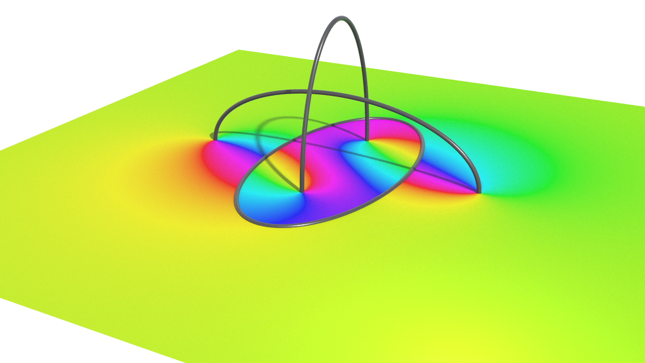
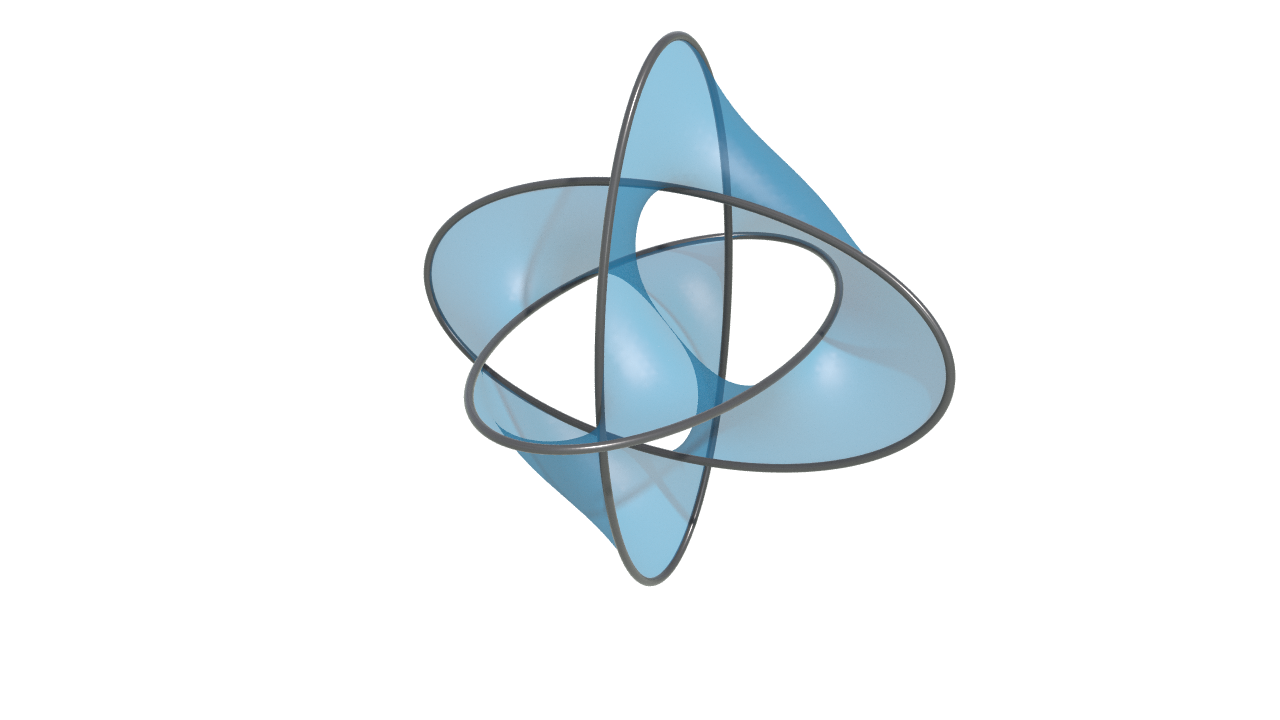
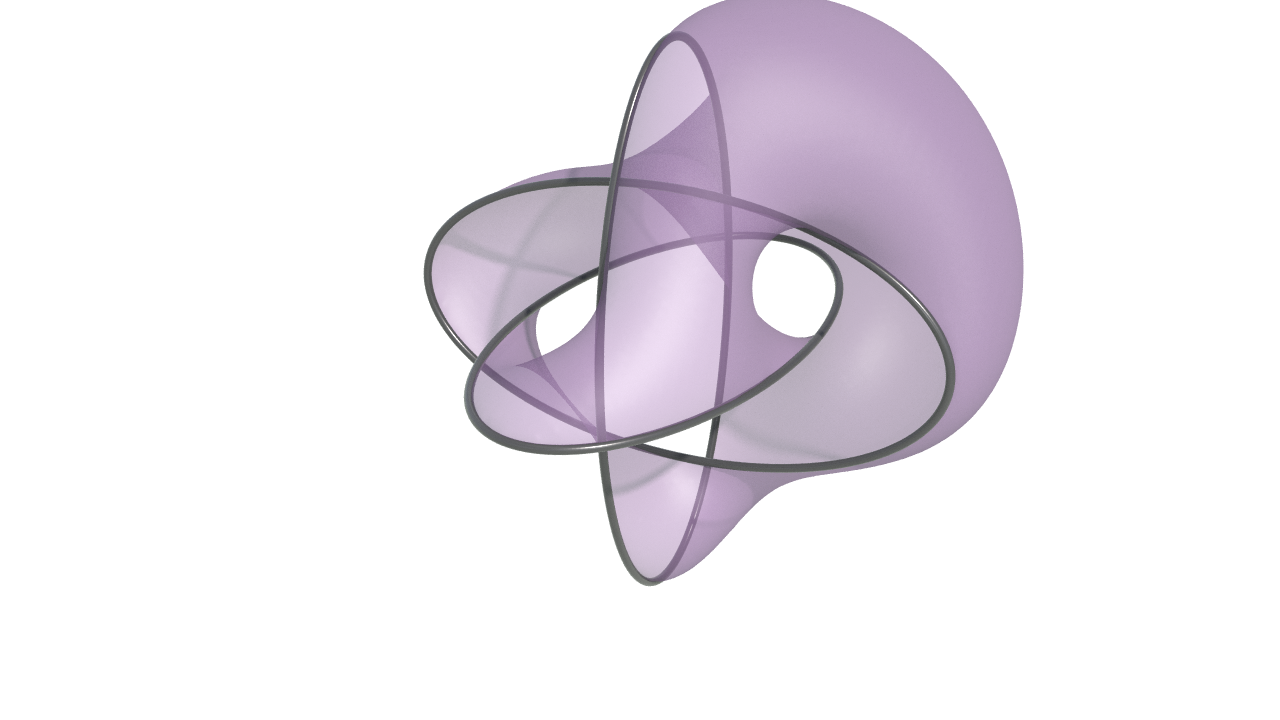
Figure 1: Left: Visualization of an implicit representation $\psi\in\mathcal{F}$ on the plane $z=0$ in $\mathbb{R}^{3}$ for a Borromean ring $\gamma\in\mathcal{X}$. Each color represents a phase i.e., the preimage of an element $s\in\SS^{1}$ under the phase map $\phi=\psi/|\psi|$. Middle and right: Visualizations of the preimages of two distinct elements in $\SS^{1}$ as surfaces bordered by $\operatorname{im}\gamma=\psi^{-1}(0)$. These preimages have codimension 1, and their intersection has codimension 2, representing $\operatorname{im}\gamma$.

Existence of implicit representations

The fibration $\Pi\colon\mathcal{F}\to\mathcal{X}$ is not surjective. More precisely, our implicit representation of shapes is limited to codimension-2 submanifolds that are exact in homology; that is, each $\gamma$ must be the boundary of an oriented codimension-1 submanifold $\Sigma$.

In this case, we can construct a map $\theta\colon M\setminus\operatorname{im}\gamma\to\mathbb{T}^{1}$ as the solution to the Dirichlet boundary problem:

$$\Delta\theta(x)=0\quad\text{for }x\notin\Sigma,$$ (4.2)

$$\theta(x)\to 2\pi\quad\text{as }x\to\Sigma_{\mathrm{f}},$$ (4.3)

$$\theta(x)\to 0\quad\ \ \text{as }x\to\Sigma_{\mathrm{b}},$$ (4.4)

where $\Sigma_{\mathrm{f}}$ and $\Sigma_{\mathrm{b}}$ denote the front and back sides of $\Sigma$, respectively. Given any smooth non-negative function $\rho$ such that $\rho^{-1}(0)=\operatorname{im}\gamma$, we can define an implicit representation $\psi$ by $\psi(x)=\rho(x)e^{i\theta(x)}$. For $M=\SS^{m}$, viewed as the one-point compactification of $\mathbb{R}^{m}$, the so-called solid angle field (visualized in Figure 1) is a special case of such a phase field $e^{i\theta}$ [BDR20, CI24].

Remark 4.1.

In this article, we consider unlabeled shapes by taking the quotient of $\mathrm{Emb}(S,M)$ by $\operatorname{Diff}^{+}(S)$, rather than by $\operatorname{Diff}_{0}(S)$, as noted in Section 3.1. Our implicit representations are naturally suited to this setting, since the level set of each $\psi$ is unlabeled and unparametrized, yet having the orientation as explained above.

Remark 4.2 (Relation with open book decomposition).

Each $\psi\in\mathcal{F}$ can be interpreted as a (relaxed) instance of an open book decomposition in contact geometry: a decomposition of the ambient manifold $M$ into an $m-2$ dimensional submanifold $B$ called the binder, and a family of $m-1$ dimensional submanifolds $\{\Sigma_{s}\}_{s\in\SS^{1}}$, called pages, such that $\partial\Sigma_{s}=B$ for each $s\in\SS^{1}$ [Gei08, Etn05].

For a given $\psi\in\mathcal{F}$, if the phase map $\phi\colon M\setminus\psi^{-1}(0)\to\SS^{1}$, defined by $\phi(x)=\frac{\psi(x)}{|\psi(x)|}$ is a submersion, then the zero set $\{\psi=0\}$ serves as the binder, and the level sets $\{\phi^{-1}(s)\}_{s\in\SS^{1}}$ form the pages. Even if $\phi$ fails to be a submersion, its level sets still form a foliation of $M$, and almost every $s\in\SS^{1}$ is a binder by Sard’s theorem.

Orbit space

The full space $\mathcal{F}$ is large and, in particular, consists of multiple connected components. Just as in the case of the explicit representation space $\mathcal{X}$, where each connected component is a $\operatorname{Diff}_{0}(M)$-orbit $\mathcal{O}$, we focus here on a single orbit $\mathcal{U}\subset\mathcal{F}$ under the action of the following group.

We define the semi-direct product group

$$\operatorname{\operatorname{DC}}\coloneqq\operatorname{Diff}_{0}(M)\ltimes\operatorname{Exp}(C^{\infty}(M,\mathbb{C})),$$ (4.5)

where $\operatorname{Diff}_{0}(M)$ acts on $\operatorname{Exp}(C^{\infty}(M,\mathbb{C}))\coloneqq\{e^{\varphi}\mid\varphi\in C^{\infty}(M,\mathbb{C})\}$ via

$$f\rhd e^{\varphi}=e^{\varphi}\circ f^{-1},\quad f\in\operatorname{Diff}_{0}(M),e^{\varphi}\in\operatorname{Exp}(C^{\infty}(M,\mathbb{C})).$$ (4.6)

The Lie group $\operatorname{\operatorname{DC}}$ has a Lie algebra $\operatorname{\mathfrak{DC}}=\operatorname{diff}(M)\ltimes C^{\infty}(M,\mathbb{C})$ with Lie bracket

$$[(u,a),(v,b)]=([u,v],-\mathcal{L}_{u}b+\mathcal{L}_{v}a),\quad u,v\in\operatorname{diff}(M),\;a,b\in C^{\infty}(M,\mathbb{C}),$$ (4.7)

where $[u,v]$ denotes the Lie bracket of vector fields on $M$.

Proposition 4.3.

The operation $\operatorname{\mathfrak{DC}}\times\operatorname{\mathfrak{DC}}\to\operatorname{\mathfrak{DC}}$ given in (4.7) defines a Lie bracket i.e., it is a bilinear skew-symmetric form satisfying the Jacobi identity.

Proof.

These properties can be verified by a straightforward computation. ∎

We now define an $\operatorname{\operatorname{DC}}$-action on $\mathcal{F}$ by

$$(f,e^{\varphi})\rhd\psi=(\psi\circ f^{-1})\cdot e^{\varphi},\quad(f,e^{\varphi})\in\operatorname{\operatorname{DC}},\psi\in\mathcal{F}.$$ (4.8)

Let $\mathcal{U}_{\psi}\subset\mathcal{F}$ denote the $\operatorname{\operatorname{DC}}$-orbit containing $\psi\in\mathcal{F}$. The tangent space at $\psi$ is

$$T_{\psi}\mathcal{U}_{\psi}=\{-\mathcal{L}_{u}\psi+\varphi\psi\mid(u,\varphi)\in\operatorname{\mathfrak{DC}}\}.$$ (4.9)

Given $\gamma=\Pi\psi\in\mathcal{X}$ and $\dot{\psi}=-\mathcal{L}_{v}\psi+\varphi\psi\in T_{\psi}\mathcal{U}_{\psi}$, we have $d\Pi(\dot{\psi})=v\circ\gamma\in T_{\gamma}\mathcal{X}$. Using the identification of $\mathcal{X}$ with de Rham currents $\mathcal{D}_{\mathcal{X}}$, this becomes $d\Pi(\dot{\psi})=-\mathcal{L}_{v}\delta_{\gamma}\in T_{\delta_{\gamma}}\mathcal{D}_{\mathcal{X}}$. Hence, we obtain

$$\Pi(\mathcal{U}_{\psi}) =\mathcal{O}_{\Pi\psi},$$ (4.10)

$$d\Pi(T_{\psi}\mathcal{U}_{\psi}) =T_{\Pi\psi}\mathcal{O}_{\Pi\psi},$$ (4.11)

where $\mathcal{O}_{\Pi\psi}$ is the $\operatorname{Diff}_{0}(M)$-orbit of $\Pi\psi\in\mathcal{X}$.

For the remainder of the paper, we denote these orbits simply by $\mathcal{U}\subset\mathcal{F}$ and $\mathcal{O}\subset\mathcal{X}$ (or $\mathcal{D}_{\mathcal{O}}\subset\mathcal{D}_{\mathcal{X}}$ under the identification), without specifying a subscript $\psi$ or $\gamma$ for indicating a particular orbit.

Remark 4.4.

The semi-direct product group $\operatorname{\operatorname{DC}}=\operatorname{Diff}_{0}(M)\ltimes\operatorname{Exp}(C^{\infty}(M,\mathbb{C}))$ is the simplest extension of $\operatorname{Exp}(C^{\infty}(M,\mathbb{C}))$ by $\operatorname{Diff}_{0}(M)$. That is, there is a split short exact sequence of groups

$$1\to\operatorname{Exp}(C^{\infty}(M,\mathbb{C}))\to\operatorname{\operatorname{DC}}\to\operatorname{Diff}_{0}(M)\to\operatorname{id}_{M}.$$ (4.12)

On $\mathcal{F}$, the group $\operatorname{\operatorname{DC}}$ acts analogously to Euclidean transformations, combining rotation and translation. The composition rule is

$$(f_{2},e^{\varphi_{2}})\circ(f_{1},e^{\varphi_{1}})=\left(f_{2}\circ f_{1},(e^{\varphi_{1}}\circ f_{2}^{-1})\cdot e^{\varphi_{2}}\right),$$ (4.13)

and $\operatorname{id}_{M}\ltimes\operatorname{Exp}(C^{\infty}(M,\mathbb{C}))$ is a normal subgroup in $\operatorname{\operatorname{DC}}$.

4.2 Geometry of fibers

In this subsection, we study the geometry of the fiber bundle $\Pi^{-1}\mathcal{O}$ consisting of implicit representations over a $\operatorname{Diff}_{0}(M)$-orbit $\mathcal{O}$ of explicit representations, as well as the geometry of a $\operatorname{\operatorname{DC}}$-orbit $\mathcal{U}$ within $\Pi^{-1}\mathcal{O}$. In particular, we show that while $\mathcal{U}$ is path-connected, each fiber may have multiple connected components, and the number of these components equals the rank of the first integral de Rham cohomology group of $M$.

We define a fiber-preserving group action on $\Pi^{-1}\mathcal{O}$. For each $\gamma\in\mathcal{O}$, let $\operatorname{Diff}_{\gamma}(M)$ be the subgroup of $\operatorname{Diff}_{0}(M)$ consisting of diffeomorphisms $f$ for which there exists a path $\{f_{t}\}_{t\in[0,1]}\subset\operatorname{Diff}_{0}(M)$ such that $f_{t}\circ\gamma=\gamma$ for all $t\in[0,1]$, with $f_{0}=\operatorname{id}_{M}$ and $f_{1}=f$. Then $\operatorname{\operatorname{DC}}_{\gamma}\coloneqq\operatorname{Diff}_{\gamma}(M)\ltimes\operatorname{Exp}(C^{\infty}(M,\mathbb{C}))$ acts on $\mathcal{U}$ as a subgroup of $\operatorname{\operatorname{DC}}$, preserving each fiber $\Pi^{-1}\gamma$. This action is clearly free on each fiber, and it turns out to be transitive on each connected component of the fiber.

We emphasize that both components of the $\operatorname{\operatorname{DC}}_{\gamma}$-action, $\operatorname{Diff}_{\gamma}(M)$ and $\operatorname{Exp}(C^{\infty}(M,\mathbb{C}))$, must work together to achieve connected component-wise transitivity. Indeed, $\mathcal{U}_{\gamma}\coloneqq\Pi^{-1}\gamma\cap\mathcal{U}$ (and hence $\Pi^{-1}\gamma$) may not be attained by the action of either $\operatorname{Exp}(C^{\infty}(M,\mathbb{C}))$ or $\operatorname{Diff}_{\gamma}(M)$ alone, as illustrated in the following examples.

Example 4.5 (Non-transitivity of $\operatorname{Diff}_{\gamma}(M)$-action).

Let $\gamma$ be four points $\{z_{k}\}_{k=1}^{4}$ on $M=\mathbb{R}^{2}$ where where $z_{1},z_{2}$ have positive orientations and $z_{3},z_{4}$ have negative orientations. We then let $\psi_{0}$ be an implicit representation of $\gamma$ defined by $\psi_{0}(z)=(z-z_{1})(z-z_{2})(\overline{z-z_{3}})(\overline{z-z_{4}})$, and $\psi_{1}\coloneqq\psi_{0}e^{i\pi/2}$ as illustrated in Figure 2. These two functions clearly lie in the same fiber $\Pi^{-1}\gamma$, but there is no diffeomorphism $f$ such that $\psi_{1}=\psi_{0}\circ f$ resolving the topological differences of the phase level sets. In contrast, the group action of $e^{i\pi/2}\in\operatorname{Exp}(C^{\infty}(M,\mathbb{C}))$ joins $\psi_{0}$ and $\psi_{1}$.

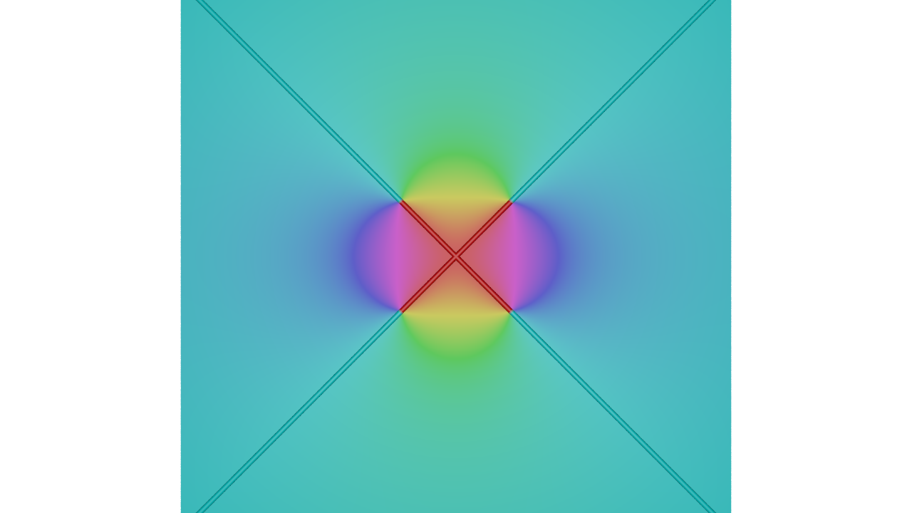
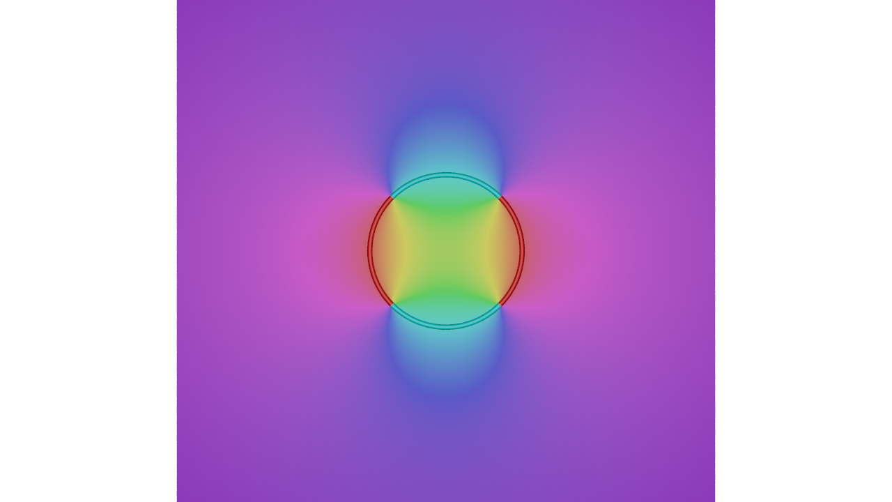
Figure 2: Implicit representations $\psi_{0}$ (left) and $\psi_{1}=\psi_{0}e^{i\frac{\pi}{2}}$ (right) of four points in $\mathbb{R}^{2}$. Each color indicates a phase value of $\phi=\psi/|\psi|$. The highlighted light-blue and red curves correspond to the level sets $\phi^{-1}(1)$ and $\phi^{-1}(e^{i\pi})$, respectively. Clearly, there is no diffeomorphism $f$ such that $\psi_{0}\circ f=\psi_{1}$ that can handle the topological changes in these level sets.

Example 4.6 (Non-transitivity of $\operatorname{Exp}(C^{\infty}(M,\mathbb{C}))$-action).

Let $M=\mathbb{R}^{2}$, and consider implicit representations $\psi_{0},\psi_{1}$ defined by $\psi_{0}(x,y)=x+iy$ and $\psi_{1}(x,y)=x+y+iy$. These functions share the same zero at $(x,y)=(0,0)$ and the same orientation. However, there is no nowhere-vanishing smooth function $\varphi$ such that $\psi_{1}=\varphi\psi_{0}$. Indeed, the quotient $\frac{\psi_{1}}{\psi_{0}}=1+\frac{xy}{x^{2}+y^{2}}-i\frac{y^{2}}{x^{2}+y^{2}}$ is discontinuous at the origin. On the other hand, with the diffeomorphism $f(x,y)=(x-y,y)$, we attain $\psi_{1}=\psi_{0}\circ f$.

The non-transitivity of the $\operatorname{Diff}_{\gamma}(M)$-action and the $\operatorname{Exp}(C^{\infty}(M,\mathbb{C}))$-action separately holds on any ambient manifold $M$, as it is caused solely by local information of implicit representations near the zero level set. For instance, on $M=\SS^{2}$ regarded as the one-point compactification of $\mathbb{R}^{2}$, the same choice of pairs $\psi_{0},\psi_{1}$ as in Section 4.2 and Section 4.2 works, with the modification that $|\psi_{0}|$, $|\psi_{1}|\to 1$ at infinity so that they are smooth functions on $\SS^{2}$.

We now show that the action of $\operatorname{\operatorname{DC}}_{\gamma}$ is indeed transitive on each connected component of the fiber $\Pi^{-1}\gamma$, and that the number of connected components is determined by the topology of the ambient manifold. Let $H^{1}_{dR}(M,\mathbb{Z})$ be the first integral de Rham cohomology defined by

$$H^{1}_{dR}(M,\mathbb{Z})=\left\{[\eta]\in H^{1}_{dR}(M,\mathbb{R})\;\middle|\;\int_{\sigma}\eta\in\mathbb{Z}\ \text{ for any }[\sigma]\in H_{1}(M,\mathbb{Z})\right\}.$$

Then we have the following relation;

Proposition 4.7.

For each $\gamma\in\mathcal{O}$, we have a bijection

$$\Pi^{-1}\gamma\big{/}\operatorname{\operatorname{DC}}_{\gamma}\cong H^{1}_{dR}(M,\mathbb{Z}).$$

To prove the proposition and highlight the roles of $\operatorname{Diff}_{\gamma}(M)$-action and $\operatorname{Exp}(C^{\infty}(M,\mathbb{C}))$-action separately, we introduce two equivalence classes.

Definition 4.8 (Twist class and conformal class).

We say $\psi_{0},\psi_{1}\in\Pi^{-1}\gamma$ are in the same twist class if there is a diffeomorphism $f\in\operatorname{Diff}_{\gamma}(M)$ such that $\psi_{1}=\psi_{0}\circ f$.

We say $\psi_{0},\psi_{1}\in\Pi^{-1}\gamma$ are in the same conformal class if there is a nowhere vanishing function $\zeta\in C^{\infty}(M,\mathbb{C}^{\times})$ such that $\psi_{1}=\zeta\psi_{0}$.

Figure 3: A ribbon of an implicit representation $\psi$ for the Hopf ring $\gamma$. For each regular value $s\in\SS^{1}$ of the phase field $\phi=\psi/|\psi|$, the ribbon $R_{s}$ (opaque cyan) is defined as the intersection of $\phi^{-1}(s)$ (translucent blue) and a small tubular neighborhood of $\operatorname{im}\gamma$.

Intuitively, $\psi_{0}$ and $\psi_{1}$ are in the same twist class if their ribbons (Figure 3) have the same total twists and hence are diffeomorphic to each other. On the other hand, $\psi_{0}$ and $\psi_{1}$ are in the same conformal class if they share the same shear states (i.e., the rate of phase change) around the zeros so that $\psi_{1}/\psi_{0}$ exists and smooth on the zeros.

Proof of Section 4.2.

We first claim that for each pair $\psi_{0},\psi_{1}\in\Pi^{-1}\gamma$, there exist functions $e^{\varphi_{0}},e^{\varphi_{1}}\in\operatorname{Exp}(C^{\infty}(M,\mathbb{C}))$ and a diffeomorphism $f\in\operatorname{Diff}_{\gamma}(M)$ such that $(e^{\varphi_{0}}\psi_{0})\circ f$ and $e^{\varphi_{1}}\psi_{1}$ lie in the same conformal class.

To see this, take some $\varphi_{0},\varphi_{1}\in C^{\infty}(M,\mathbb{C})$ so that, letting $\hat{\psi}_{0}\coloneqq e^{\varphi_{0}}\psi_{0}$ and $\hat{\psi}_{1}\coloneqq e^{\varphi_{1}}\psi_{1}$, we have $|\hat{\psi}_{0}|=|\hat{\psi}_{1}|$ in a small tubular neighborhood $B$ of $\operatorname{im}\gamma$, and the phase field $\hat{\phi}_{j}=\frac{\hat{\psi}_{j}}{|\hat{\psi}_{j}|}\colon B\setminus\operatorname{im}\gamma\to\SS^{1}$ is a submersion for $j=0,1$.

We can take coordinates $(p,z)$ in $B$ with $p\in\operatorname{im}\gamma$ and $z\coloneqq\hat{\psi}_{0}(p,\cdot)$. Then consider a tubular sub-neighborhood $B_{R}=\{(p,z)\mid p\in\operatorname{im}\gamma,|z|\leq R\}$ small enough so that $\hat{\psi}_{1}$ is injective on each circle $S_{p}^{\epsilon}=\{(p,z)\mid|z|=\epsilon\}$ for $p\in\operatorname{im}\gamma$ and $\epsilon\leq R$. Then for a sufficiently small $r<R$, there exists $f\in\operatorname{\operatorname{DC}}_{\gamma}$ such that $\hat{\psi}_{0}\circ f=\tau\hat{\psi}_{1}$ inside the smaller tubular neighborhood $B_{r}=\{(p,z)\mid p\in\operatorname{im}\gamma,|z|\leq r\}$ and $f=\operatorname{id}$ outside $B_{R}$, as illustrated in Figure 4. Here $\tau$ is a smooth function on $B_{r}$ of the form $\tau(p,z)=e^{i\theta(p)}$ with some $\mathbb{T}^{1}$-valued function $\theta$.

Outside $B_{r}$, the function $\frac{\hat{\psi}_{1}}{\hat{\psi}_{0}\circ f}$ is smooth and nowhere vanishing. Hence there exists a smooth function $\zeta\in C^{\infty}(M,\mathbb{C}^{\times})$ such that $\hat{\psi}_{0}\circ f=\zeta\hat{\psi}_{1}$ and $\zeta=\tau$ inside $B_{r}$, showing that $\psi_{0}\circ f$ and $\psi_{1}$ are in the same conformal class.

We now note that the following is an exact sequence:

$$0\to\mathbb{Z}\xrightarrow[]{k\mapsto 2\pi ik}C^{\infty}(M,\mathbb{C})\xrightarrow[]{\exp}C^{\infty}(M,\mathbb{C}^{\times})\xrightarrow[]{\mathfrak{h}}H^{1}_{dR}(M,\mathbb{Z})\to 0$$ (4.14)

where $\mathfrak{h}\colon C^{\infty}(M,\mathbb{C}^{\times})\to H^{1}_{dR}(M,\mathbb{Z})$ is defined by $\mathfrak{h}(\kappa)=\left[\operatorname{Im}\frac{1}{2\pi}\frac{d\kappa}{\kappa}\right]$. Therefore $\zeta$ defines an element $\mathfrak{h}(\zeta)\in H^{1}_{dR}(M,\mathbb{Z})$, and the functions $\hat{\psi}_{0}\circ f$ and $\hat{\psi}_{1}$ are in the same twist class if and only if $\mathfrak{h}(\zeta)=[0]$.

On the other hand, each pair of elements $[\eta_{1}],[\eta_{2}]\in H^{1}_{dR}(M,\mathbb{Z})$ define elements $[\zeta_{1}],[\zeta_{2}]\in C^{\infty}(M,\mathbb{C}^{\times})/\operatorname{Exp}(C^{\infty}(M,\mathbb{C}))$ such that $\zeta_{1}\psi$ and $\zeta_{2}\psi$ for any choice of $\psi\in\Pi^{-1}\gamma$, and the representatives $\zeta_{1},\zeta_{2}$ are in the same $\operatorname{\operatorname{DC}}_{\gamma}$-orbit if and only if $[\eta_{1}]=[\eta_{2}]$. This completes the proof. ∎

Hence we have shown that, while a $\operatorname{\operatorname{DC}}$-orbit $\mathcal{U}$ is path connected, each fiber $\Pi^{-1}\gamma$ consists of a disjoint copies of a $\operatorname{\operatorname{DC}}_{\gamma}$-orbit associated with the discrete group $H^{1}_{dR}(M,\mathbb{Z})$.

$\hat{\psi}_{0}(p,z)=z$

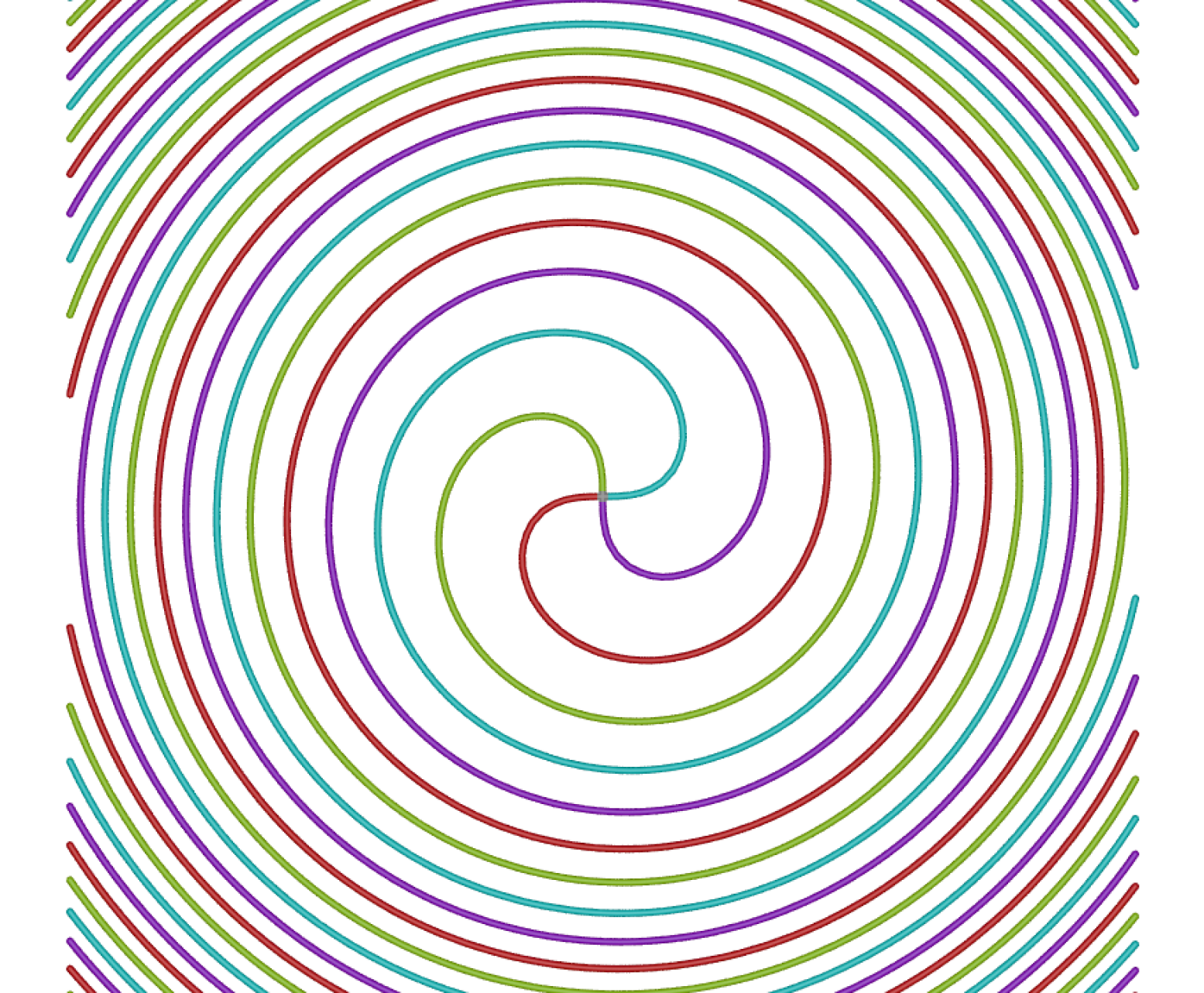
$\hat{\psi}_{1}(p,z)=ze^{i|z|^{2}}$

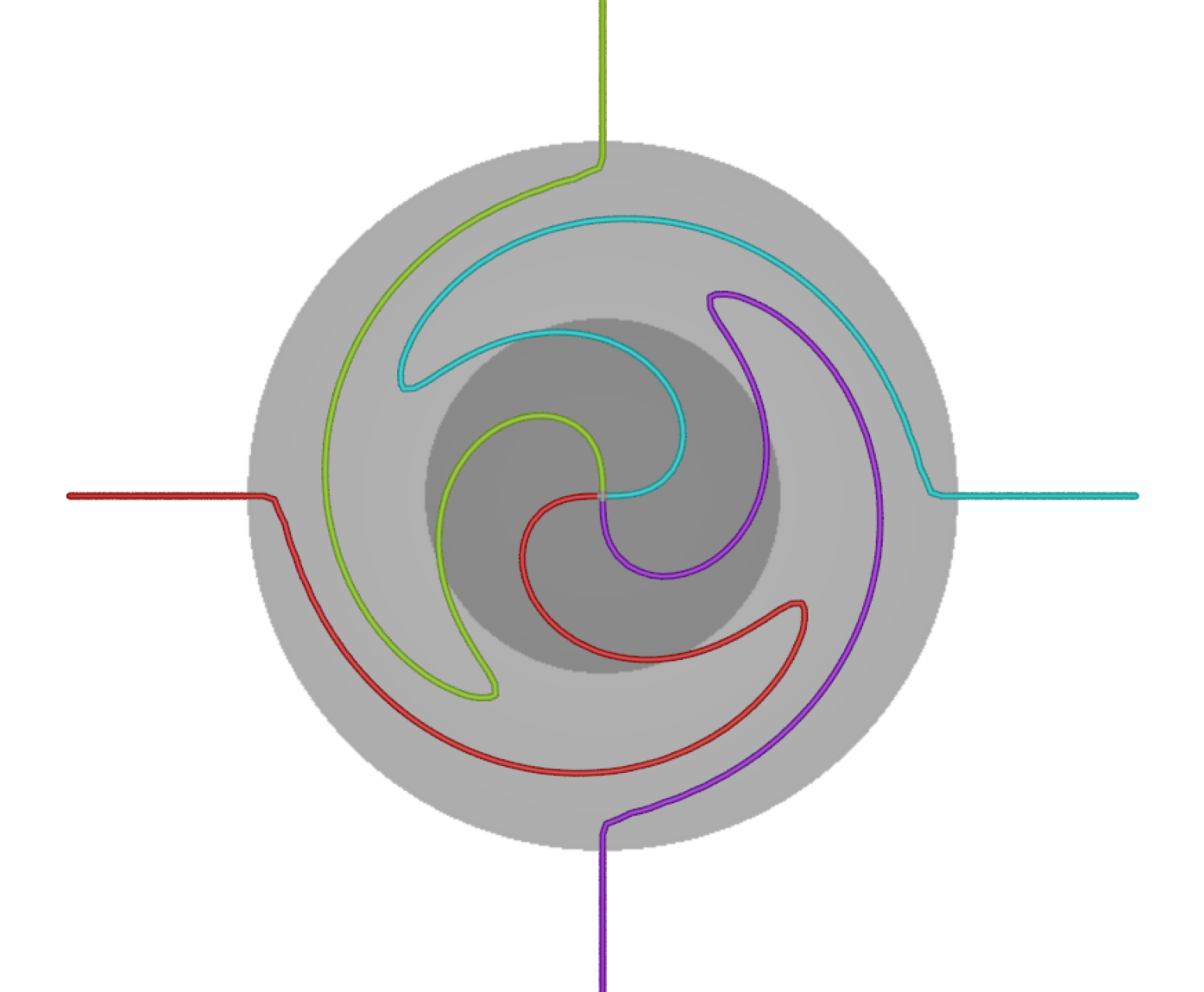
$\hat{\psi}_{0}\circ f$

Figure 4: Level curves $\hat{\phi}^{-1}(1),\hat{\phi}^{-1}(e^{i\frac{\pi}{2}}),\hat{\phi}^{-1}(-1),\hat{\phi}^{-1}(e^{i\frac{3\pi}{2}})$ of the phase maps $\hat{\phi}=\hat{\psi}/|\hat{\psi}|$ of implicit representations $\hat{\psi}_{0}(p,z)=z$ (left), $\hat{\psi}_{1}(p,z)=ze^{i|z|^{2}}$ (middle), and $\hat{\psi}_{0}\circ f$ (right), on the tubular domain $B$ sliced into a disc at fixed $p\in\operatorname{im}\gamma$. The diffeomorphism $f$ rotates these level lines on each circle $S^{\epsilon}_{p}=\{(p,z)\mid|z|=\epsilon\}$ for $\epsilon\leq R$ so that $\hat{\psi}_{0}\circ f$ agrees with $\hat{\psi}_{1}$ inside the smaller domain $B_{r}$ (dark gray) and with $\hat{\psi}_{0}$ outside the larger domain $B_{R}$ (light gray).

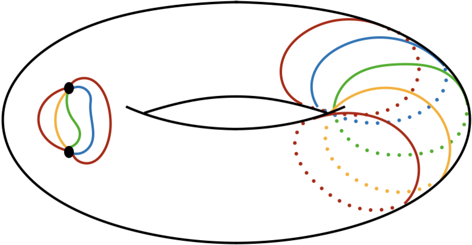
$\psi_{0}$

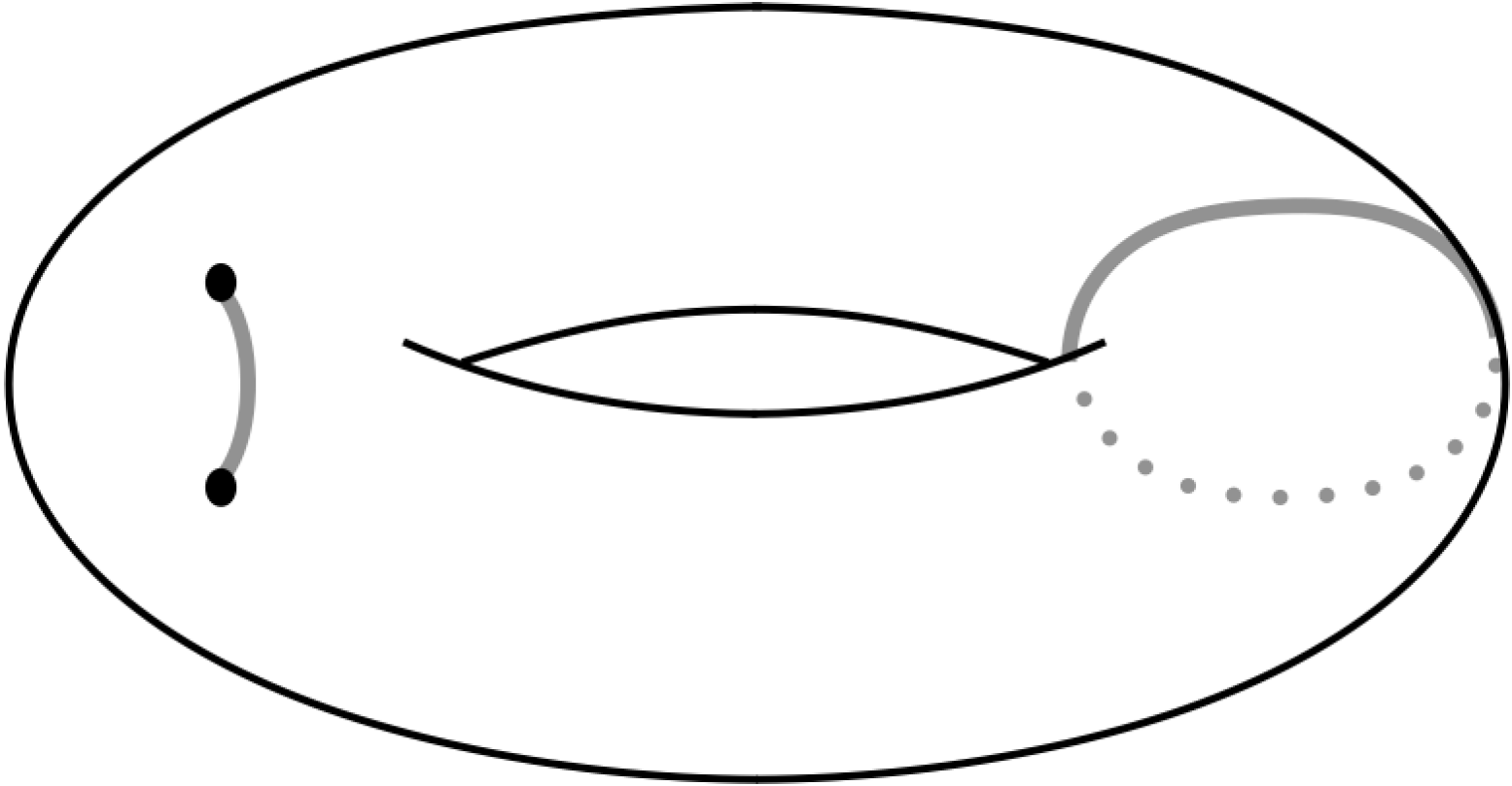
$\psi_{t_{1}}$

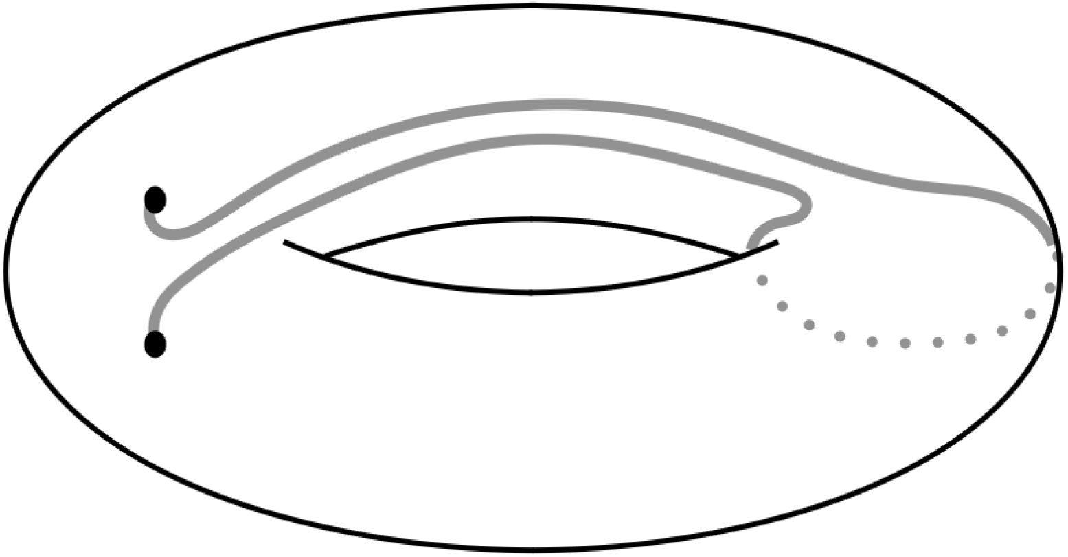
$\psi_{t_{2}}$

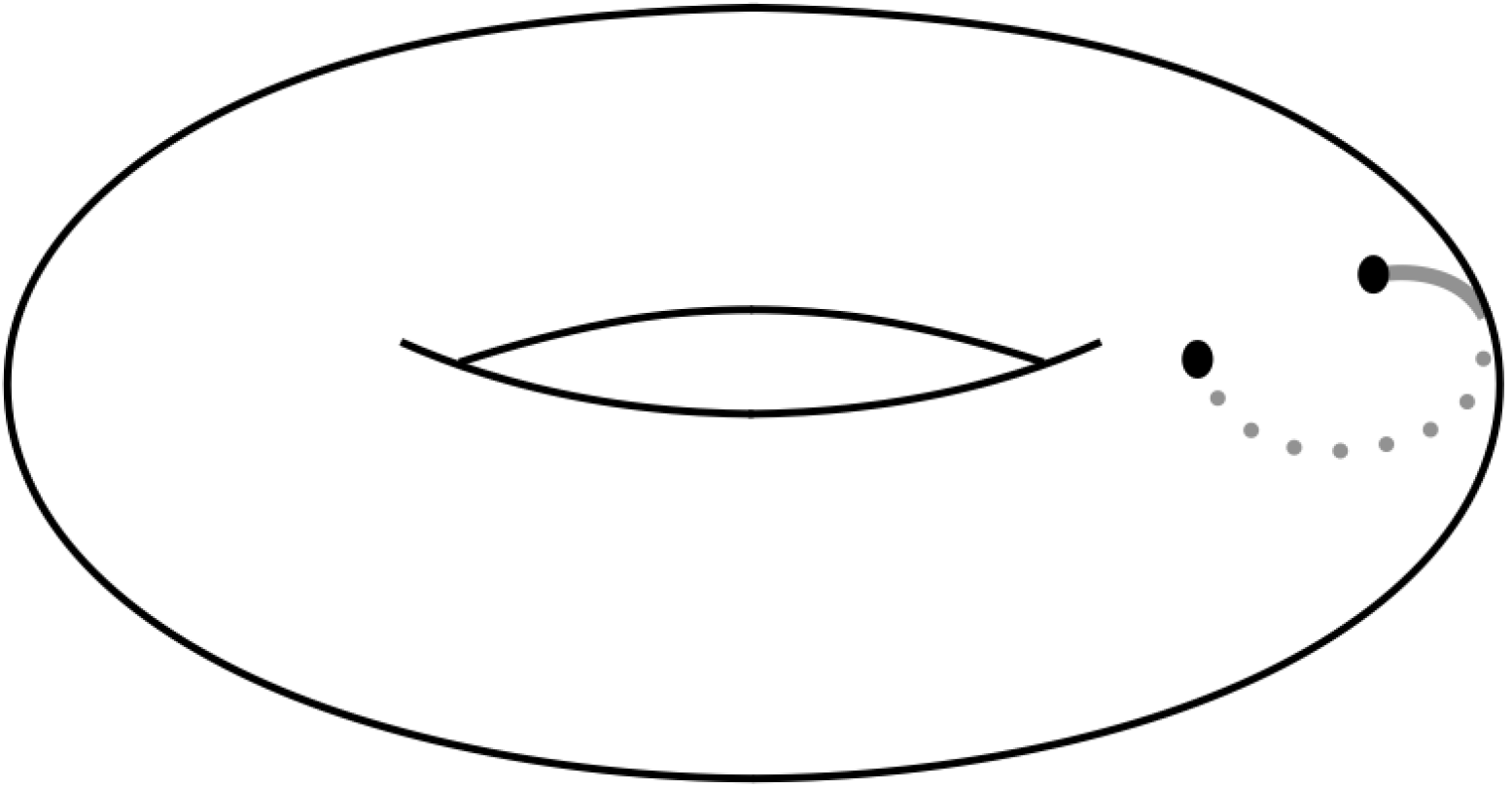
$\psi_{t_{3}}$

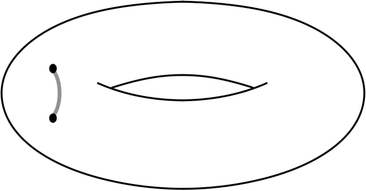
$\psi_{t_{4}}$

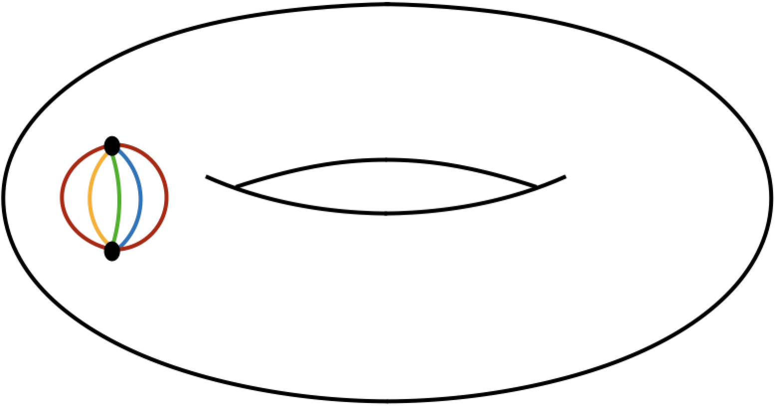
$\psi_{1}$

Figure 5: A transition of the implicit representation from $\psi_{0}$ (top left) to $\psi_{1}$ (bottom right) for two points $\gamma$ on the torus $\mathbb{T}^{2}$. In both $\psi_{0}$ and $\psi_{1}$, the colored curves represent level sets $\phi^{-1}(s)$ of some phases. Clearly, $\psi_{0}$ and $\psi_{1}$ belong to different connected components of the fiber $\pi^{-1}\gamma$. Nevertheless, they lie on the same $\operatorname{\operatorname{DC}}$-orbit. Starting from $\psi_{0}$, we first multiply by some $e^{\varphi_{1}}\in\operatorname{Exp}(\mathbb{C}^{\infty}(M,\mathbb{C}))$ to compress the support of $d\phi$ into narrow bands, visualized as thick gray curves in $\psi_{t_{1}}$. Next, multiplying $\psi_{t_{1}}$ by $e^{\varphi_{2}}\in\operatorname{Exp}(\mathbb{C}^{\infty}(M,\mathbb{C}))$ merges two level curves, producing $\psi_{t_{2}}$. Applying a diffeomorphism $f_{1}$ moves the level lines, yielding $\psi_{t_{3}}$, and a second diffeomorphism $f_{2}$ transforms $\psi_{t_{3}}$ into $\psi_{t_{4}}$. Finally, multiplying by another $e^{\varphi_{3}}\in\operatorname{Exp}(\mathbb{C}^{\infty}(M,\mathbb{C}))$ decompresses the support of $d\phi$, resulting in $\psi_{1}$.

Is the fiber bundle $\mathcal{F}_{\mathcal{O}}\coloneqq\Pi^{-1}\mathcal{O}$ larger than a single orbit $\mathcal{U}$?

Since each fiber $\Pi^{-1}\gamma$ is an orbit of $\operatorname{Diff}_{\gamma}\ltimes C^{\infty}(M,\mathbb{C}^{\times})$, the entire fiber bundle $\mathcal{F}_{\mathcal{O}}\coloneqq\Pi^{-1}\mathcal{O}$ over a fixed $\mathcal{O}$ is a $\operatorname{Diff}_{0}(M)\ltimes C^{\infty}(M,\mathbb{C}^{\times})$-orbit. As each fiber has multiple connected components when $H^{1}_{dR}(M,\mathbb{Z})\neq 0$, the fiber bundle $\mathcal{F}_{\mathcal{O}}$ appears to be strictly larger than $\mathcal{U}$, a single orbit under the action of $\operatorname{\operatorname{DC}}=\operatorname{Diff}_{0}(M)\ltimes\operatorname{Exp}(C^{\infty}(M,\mathbb{C}))$. It, however, turns out that $\mathcal{F}_{\mathcal{O}}=\mathcal{U}$ at last for the case of the base dimension 2 as illustrated in Figure 5. By moving around zeros while multiplying functions in $\operatorname{Exp}(C^{\infty}(M,\mathbb{C}))$, we can overcome topological changes of phase level lines. We expect that a similar argument holds in higher dimensional cases and the result remains valid:

Conjecture 4.9.

Let $\mathcal{O}$ be a $\operatorname{Diff}_{0}(M)$-orbit in the explicit shape space $\mathcal{X}$, $\mathcal{F}_{\mathcal{O}}\coloneqq\Pi^{-1}\mathcal{O}$ be the entire fiber bundle over $\mathcal{O}$, and $\mathcal{U}$ be a $\operatorname{\operatorname{DC}}$-orbit in $\mathcal{F}_{\mathcal{O}}$. Suppose each connected component of $M$ intersects with $\operatorname{im}\gamma$ for $\gamma\in\mathcal{O}$. Then $\mathcal{F}_{\mathcal{O}}=\mathcal{U}$.

We conclude this subsection by observing that an $\operatorname{Diff}_{0}(M)\ltimes C^{\infty}(M,\mathbb{C}^{\times})$-orbit $\mathcal{F}_{\mathcal{O}}$ is locally a $\operatorname{\operatorname{DC}}$-orbit $\mathcal{U}$ and they share the same tangent space at each $\psi$ even if $\mathcal{U}\subsetneq\mathcal{F}_{\mathcal{O}}$. In this section and the next section, we still focus on local arguments on $\mathcal{U}$, which are all available on $\mathcal{F}_{\mathcal{O}}$ when we consider prequantum $G$-bundles in Section 6.

5 Liouville form in the prequantum sense

In this section, we present one of our main results: the MW symplectic form $\omega$ on $\mathcal{O}$ over a general closed manifold $M$ admits a Liouville form in the prequantum sense. In this section and the rest of the article, we assume that the ambient manifold $M$ is closed, in contrast to the setting in Section 3 for the explicit shape space.

Definition 5.1.

Define the following 1-form on each $\operatorname{\operatorname{DC}}$-orbit $\mathcal{U}$ of $\mathcal{F}$:

$$\Theta_{\psi}(\dot{\psi})=\frac{1}{2\pi}\int_{M}\operatorname{Im}\frac{\dot{\psi}\bar{\psi}}{|\psi|^{2}}\ \mu,$$ (5.1)

where $\dot{\psi}=-\mathcal{L}_{u}\psi+\varphi\psi\in T_{\psi}\mathcal{U}$ for some $(u,\varphi)\in\operatorname{\mathfrak{DC}}$.

At first glance, the integral in (5.1) may appear divergent as the integrand is unbounded near the zeros of $\psi$. However, we will show that it is in fact finite. We also demonstrate that the value $\Theta_{\psi}(\dot{\psi})$ has a clear physical interpretation (Section 5).

Definition 5.2 (Formal prequantization and Liouville form).

Let $(B,\beta)$ be a symplectic manifold, and let $E$ be a manifold equipped with a 1-form $\alpha$. We say that a fibration $\pi\colon E\to B$ is a formal prequantization, and that $\alpha$ is a Liouville form of $\beta$ in the prequantum sense, if

$$d\alpha=\pi^{*}\beta.$$ (5.2)

Theorem 5.3 (Liouville form for the MW structure in the prequantum sense).

Suppose $M$ is a closed manifold equipped with a volume form $\mu$. Then the fibration $\Pi\colon(\mathcal{U},\Theta)\to(\mathcal{O},\omega)$ is a formal prequantization.

Proof strategy

To prove the theorem, that is, to show $d\Theta=\Pi^{*}\omega$, we combine a standard approach in differential geometry with the coarea formula from geometric measure theory. We compute the exterior derivative of $\Theta_{\psi}$ by the formula

$$d\Theta_{\psi}(\dot{\psi},\ring{\psi})=\mathcal{L}_{Y_{1}}\iota_{Y_{2}}\Theta_{\psi}-\mathcal{L}_{Y_{2}}\iota_{Y_{1}}\Theta_{\psi}-\iota_{[Y_{1},Y_{2}]}\Theta_{\psi}$$ (5.3)

for each $\psi\in\mathcal{U}$ and $\dot{\psi},\mathring{\psi}\in T_{\psi}\mathcal{U}$. Here, the vector fields $Y_{1},Y_{2}\in\Gamma(T\mathcal{U})$ are arbitrary extensions of the vectors $\dot{\psi},\mathring{\psi}$ respectively; that is, $Y_{1}|_{\psi}=\dot{\psi}$ and $Y_{2}|_{\psi}=\mathring{\psi}$.

To perform this calculation, we first choose specific vector fields $Y_{1}$ and $Y_{2}$ and explicitly compute each term in (5.3). This calculation leads to a simple expression of $d\Theta$ (Section 5). As the final step of the proof, we show that the fibration $\Pi:\mathcal{U}\to\mathcal{D}_{\mathcal{O}}\subset\mathcal{D}_{m-2}(M)$ is decomposed into $\Pi=\partial\circ\Lambda$ (Section 5) using the coarea formula, where the map $\Lambda\colon\mathcal{U}\to\mathcal{D}_{m-1}(M)$ assigns to each $\psi$ its circle differential $(m-1)$-current, as defined below (Section 5), and $\partial\colon\mathcal{D}_{m-1}(M)\to\mathcal{D}_{m-2}(M)$ is the boundary operator for currents.

Definition 5.4 (Circle differential 1-form and $(m-1)$-current).

Using the normalization map $\tau\colon\mathbb{C}^{\times}\to\SS^{1}$ given by $z\mapsto\frac{z}{|z|}$ and the standard Haar measure $\sigma\in\Omega^{1}(\SS^{1})$ on $\SS^{1}$ with normalization $\int_{\SS^{1}}\sigma=1$, define the circle differential 1-form $\lambda_{\psi}\in\Omega^{1}(M\setminus\psi^{-1}(0))$ by

$$\lambda_{\psi}\coloneqq\psi^{*}\tau^{*}\sigma.$$ (5.4)

This induces the map $\Lambda\colon\mathcal{F}\to\mathcal{D}_{m-1}(M)$ by

$$\langle\Lambda(\psi),\beta\rangle\coloneqq\int_{M}\lambda_{\psi}\wedge\beta,\quad\beta\in\Omega^{m-1}(M).$$ (5.5)

We call $\Lambda(\psi)$ the circle differential current.

The circle differential $\lambda_{\psi}$ represents the gradient of the phase of $\psi$. In fact, there is a small neighborhood $N_{x}$ around each point $x\in M\setminus\psi^{-1}(0)$ such that $\psi$ is locally represented by $\psi(y)=r(y)\cdot e^{i\phi(y)}$ with some function $r\colon N_{x}\to\mathbb{R}_{>0}$ and $\phi\colon N_{x}\to\mathbb{R}$ with $d\phi=\lambda_{\psi}$.

The integral (5.5) is well-defined because the integrand $\lambda_{\psi}\wedge\alpha$ is defined almost everywhere on $M$ with respect to $\mu$, in particular, except on the codimension-2 set $\psi^{-1}(0)$. In fact, $\Lambda(\psi)$ is indeed a current i.e., a continuous linear functional on $\Omega^{m-1}(M)$, and namely the value (5.5) is always finite;

Lemma 5.5.

Let $M$ be a closed manifold and $\psi\in\mathcal{F}$. Then $\Lambda(\psi)\in\mathcal{D}_{m-1}(M)$.

This result is a direct consequence of the coarea formula from geometric measure theory, which is a nonlinear version of the Fubini theorem.

Proposition 5.6 (Smooth coarea formula).

Let $X$ be an oriented smooth manifold and $Y$ be an oriented compact smooth manifold with dimension $n_{X}$ and $n_{Y}<n_{X}$ respectively. For a submersion $f\colon X\to Y$ and forms $\beta\in\Omega^{n_{X}-n_{Y}}(Y),\sigma\in\Omega^{n_{Y}}(Y)$, we have

$$\int_{X}f^{*}\sigma\wedge\beta=\int_{Y}\langle\delta_{f^{-1}(\cdot)},\beta\rangle\ \sigma.$$ (5.6)

Remark 5.7.

There are different versions of the coarea formula. Here, we use the version from [Dem97, Chapter I.3], as it is formulated in terms of differential forms and does not rely on Hausdorff measure or a Riemannian metric, making it well-suited for our context.

For standard references on the coarea formula, readers may find works like [Fed14] and [Nic11] helpful.

Proof of Section 5.

Clearly $\Lambda(\psi)$ is linear in $\mathcal{D}_{m-1}(M)$. We now show that $\Lambda(\psi)$ is a bounded functional. By the coarea formula (Section 5), we have for any $\beta\in\Omega^{m-1}(M)$ that,

$$\langle\Lambda(\psi),\beta\rangle =\int_{M}\lambda_{\psi}\wedge\beta=\int_{M^{\operatorname{reg}\phi}}\lambda_{\psi}\wedge\beta=\int_{\SS^{1}}\langle\delta_{(\phi^{-1}(\cdot)\cap M^{\operatorname{reg}\phi})},\beta\rangle\sigma$$ (5.7)

where $\phi=\tau\circ\psi\colon{M\setminus\psi^{-1}(0)}\to\SS^{1}$ and $M^{\operatorname{reg}\phi}$ denotes the set of regular points of $\phi$. Note that the set $\phi^{-1}(s)\cap M^{\operatorname{reg}\phi}$ for each $s\in\SS^{1}$ is a $m-1$ dimensional submanifold and namely $\delta_{\partial(\phi^{-1}(s)\cap M^{\operatorname{reg}\phi})}$ is a $m-1$-current. In particuluar, the operator norm $\|\delta_{\partial(\phi^{-1}(s)\cap M^{\operatorname{reg}\phi})}\|_{\mathcal{D}_{m-1}(M)}$ is bounded. Therefore,

$$\|\Lambda(\psi)\|_{\mathcal{D}_{m-1}(M)}\leq\int_{\SS^{1}}\sigma\sup_{s\in\SS^{1}}\|\delta_{\partial(\phi^{-1}(s)\cap M^{\operatorname{reg}\phi})}\|_{\mathcal{D}_{m-1}(M)}=2\pi\sup_{s\in\SS^{1}}\|\delta_{\partial(\phi^{-1}(s)\cap M^{\operatorname{reg}\phi})}\|_{\mathcal{D}_{m-1}(M)}$$

is bounded, from which we conclude that $\Lambda(\psi)$ is a current. ∎

As we see from the proof, the current $\Lambda(\psi)$ is in fact the superposition of a $\SS^{1}$-family of hypersurfaces given as the phase level sets of $\psi$.

Vector fields $Y_{1},Y_{2}\in\Gamma(T\mathcal{U})$

We now choose the vector fields $Y_{1}$ and $Y_{2}$ that extend $\dot{\psi}$ and $\mathring{\psi}$ to evaluate (5.3). As in our approach for Theorem 3.5, we use the fundamental vector field associated with the action of $\operatorname{\operatorname{DC}}=\operatorname{Diff}_{0}(M)\ltimes\operatorname{Exp}(C^{\infty}(M,\mathbb{C}))$ on $\mathcal{U}$. Recalling that the Lie algebra of $\operatorname{\operatorname{DC}}$ is $\operatorname{\mathfrak{DC}}=\operatorname{diff}(M)\ltimes C^{\infty}(M,\mathbb{C})$, we define $Y^{(u,a)}\in\Gamma(T\mathcal{U})$ for each $(u,a)\in\operatorname{\mathfrak{DC}}$ by

$$Y^{(u,a)}(\psi)\coloneqq\frac{d}{dt}\big{|}_{t=0}{\operatorname{Fl}_{u}^{-t}}^{*}\psi\cdot e^{ta}=-\mathcal{L}_{u}\psi+a\psi.$$ (5.8)

We first explicitly compute their Lie bracket;

Lemma 5.8.

For $(u,a),(v,b)\in\operatorname{\mathfrak{DC}}$ and $\psi\in\mathcal{U}$, we have

$$[Y^{(u,a)},Y^{(v,b)}](\psi)=-\mathcal{L}_{[u,v]}\psi+(\mathcal{L}_{u}b-\mathcal{L}_{v}a)\psi.$$ (5.9)

Proof.

To compute the Lie derivative of vector fields $[Y^{(u,a)},Y^{(v,b)}]=\mathcal{L}_{Y^{(u,a)}}Y^{(v,b)}$, we use the formula:

$$\mathcal{L}_{Y^{(u,a)}}Y^{(v,b)}(\psi)=\frac{d}{dt}\Big{|}_{t=0}D\Phi^{-t}_{Y^{(u,a)}}\left(Y^{(v,b)}(\Phi^{t}_{Y^{(u,a)}}(\psi))\right),\quad\psi\in\mathcal{U}$$ (5.10)

where $\Phi^{t}_{Y}\colon\mathcal{U}\to\mathcal{U}$ is the flow map along $Y\in\Gamma(T\mathcal{U})$ defined by the ODE

$$\frac{d}{dt}(\Phi^{t}_{Y}(\psi))=Y(\Phi^{t}_{Y}(\psi)),$$ (5.11)

$$\Phi^{0}_{Y}=\operatorname{id}_{\mathcal{U}},$$ (5.12)

and $D\Phi^{t}_{Y}|_{\psi}\colon T_{\psi}\mathcal{U}\to T_{\Phi^{t}_{Y}(\psi)}\mathcal{U}$ is its differential at $\psi$. For the fundamental vector field $Y^{(u,a)}$ associated to $(u,a)\in\operatorname{\mathfrak{DC}}$, we have by definition $\Phi^{t}_{Y^{(u,a)}}(\psi)={\operatorname{Fl}_{u}^{-t}}^{*}\psi\cdot e^{ta}$. Since

$$Y^{(v,b)}(\Phi^{t}_{Y^{(u,a)}}(\psi)) =\frac{d}{ds}\Big{|}_{s=0}\Phi^{s}_{Y^{(v,b)}}\left(\Phi^{t}_{Y^{(u,a)}}(\psi)\right),$$ (5.13)

we have

$$\frac{d}{dt}\Big{|}_{t=0}D\Phi^{-t}_{Y^{(u,a)}}\left(Y^{(v,b)}(\Phi^{t}_{Y^{(u,a)}}(\psi))\right) =\frac{d}{dt}\Big{|}_{t=0}\frac{d}{ds}\Big{|}_{s=0}\Phi^{-t}_{Y^{(u,a)}}\left(\Phi^{s}_{Y^{(v,b)}}\left(\Phi^{t}_{Y^{(u,a)}}(\psi)\right)\right)$$ (5.14)

$$=\frac{d}{dt}\Big{|}_{t=0}\frac{d}{ds}\Big{|}_{s=0}\Phi^{-t}_{Y^{(u,a)}}\left(\Phi^{s}_{Y^{(v,b)}}(\psi)\right)+\Phi^{s}_{Y^{(v,b)}}\left(\Phi^{t}_{Y^{(u,a)}}(\psi)\right)$$ (5.15)

using the product rule. We then compute the first term:

$$\frac{d}{dt}\Big{|}_{t=0}\frac{d}{ds}\Big{|}_{s=0}\Phi^{-t}_{Y^{(u,a)}}\left(\Phi^{s}_{Y^{(v,b)}}(\psi)\right) =\frac{d}{dt}\Big{|}_{t=0}\frac{d}{ds}\Big{|}_{s=0}{\operatorname{Fl}^{t}_{u}}^{*}\left({\operatorname{Fl}^{-s}_{v}}^{*}\psi\cdot e^{sb}\right)\cdot e^{-ta}$$ (5.16)

$$=\frac{d}{dt}\Big{|}_{t=0}\frac{d}{ds}\Big{|}_{s=0}{\operatorname{Fl}^{t}_{u}}^{*}\left({\operatorname{Fl}^{-s}_{v}}^{*}\psi\right)\cdot{\operatorname{Fl}^{t}_{u}}^{*}e^{sb}\cdot e^{-ta}$$ (5.17)

$$=\frac{d}{ds}\Big{|}_{s=0}\mathcal{L}_{u}\left({\operatorname{Fl}^{-s}_{v}}^{*}\psi\right)\cdot e^{sb}+\left({\operatorname{Fl}^{-s}_{v}}^{*}\psi\right)\mathcal{L}_{u}(e^{sb})-\left({\operatorname{Fl}^{-s}_{v}}^{*}\psi\right)\cdot e^{sb}\cdot a$$ (5.18)

$$=-\mathcal{L}_{u}\mathcal{L}_{v}\psi+\mathcal{L}_{u}\psi\cdot b-\mathcal{L}_{v}\psi\cdot 0+\psi\mathcal{L}_{u}b+\mathcal{L}_{v}\psi\cdot a-\psi\cdot b\cdot a$$ (5.19)

$$=-\mathcal{L}_{u}\mathcal{L}_{v}\psi+b\mathcal{L}_{u}\psi+a\mathcal{L}_{v}\psi+\psi\mathcal{L}_{u}b-ab\psi$$ (5.20)

where we used $\mathcal{L}_{u}(e^{sb})=s\mathcal{L}_{u}b\cdot e^{sb}$. Similarly, we have

$$\frac{d}{dt}\Big{|}_{t=0}\frac{d}{ds}\Big{|}_{s=0}\Phi^{s}_{Y^{(v,b)}}\left(\Phi^{t}_{Y^{(u,a)}}(\psi)\right)=\mathcal{L}_{v}\mathcal{L}_{u}\psi-a\mathcal{L}_{v}\psi-b\mathcal{L}_{u}\psi-\psi\mathcal{L}_{v}a+ab\psi.$$ (5.21)

Summing these results, we have

$$\frac{d}{dt}\Big{|}_{t=0}\frac{d}{ds}\Big{|}_{s=0}\Phi^{-t}_{Y^{(u,a)}}\left(\Phi^{s}_{Y^{(v,b)}}(\psi)\right)+\Phi^{s}_{Y^{(v,b)}}\left(\Phi^{t}_{Y^{(u,a)}}(\psi)\right) =-\mathcal{L}_{u}\mathcal{L}_{v}\psi+\mathcal{L}_{v}\mathcal{L}_{u}\psi+\psi\mathcal{L}_{v}b-\psi\mathcal{L}_{v}a$$ (5.22)

$$=-\mathcal{L}_{[u,v]}\psi+(\mathcal{L}_{u}b-\mathcal{L}_{v}a)\psi.$$ (5.23)

We thus obtained the stated expression. ∎

Remark 5.9.

The fundamental vector field mapping $\operatorname{\mathfrak{DC}}\to\Gamma(T\mathcal{U})$ given by (5.8) is in fact a Lie algebra anti-homomorphism. To see this, notice that the mapping $\operatorname{diff}(M)\to\operatorname{Der}(C^{\infty}(M,\mathbb{C}))$ by $u\to\mathcal{L}_{u}$ is an anti-homomorphism as noted in Section 3.4. Hence we have

$$Y^{[(u,a),(v,b)]}=Y^{([u,v],-\mathcal{L}_{u}b+\mathcal{L}_{v}a)}=\mathcal{L}_{[u,v]}\psi+(\mathcal{L}_{v}a-\mathcal{L}_{u}b)\psi=-[Y^{(u,a)},Y^{(v,b)}]$$ (5.24)

where the last equality is the application of Section 5.

Evaluation of $\Theta$ and $d\Theta$

We now evaluate each term in (5.3) with $Y_{1}=Y^{(u,a)}$ and $Y_{2}=Y^{(v,b)}$. First, we express the term $\Theta_{\psi}(Y^{(u,a)})=\Theta_{\psi}(-\mathcal{L}_{u}\psi+a\psi)$ more explicitly.

Lemma 5.10 (Evaluation of $\Theta_{\psi}$).

For any $(u,a)\in\operatorname{\mathfrak{DC}}$, we have

$$\Theta_{\psi}(-\mathcal{L}_{u}\psi+a\psi) =\Theta_{\psi}(-\mathcal{L}_{u}\psi)+\Theta_{\psi}(a\psi)$$ (5.25)

$$=\frac{1}{2\pi}\left(-\langle\Lambda(\psi),\iota_{u}\mu\rangle+\int\operatorname{Im}a\ \mu\right),$$ (5.26)

where $\Lambda(\psi)$, defined in (5.5), is the current associated to the circle differential of $\psi$, and $\mu$ is the volume form on $M$.

Proof.

By direct computation we get

$$\Theta_{\psi}(a\psi)=\frac{1}{2\pi}\int\operatorname{Im}\frac{a\psi\bar{\psi}}{|\psi|^{2}}\mu=\frac{1}{2\pi}\int\operatorname{Im}a\ \mu.$$ (5.27)

We then compute $\Theta_{\psi}(-\mathcal{L}_{u}\psi)$. Using the local expression $\psi=re^{i\phi}$ with $r=|\psi|$ and a function $\phi$ around each $x\in M\setminus\psi^{-1}(0)$, we have locally

$$d\psi=e^{i\phi}dr+re^{i\phi}id\phi$$ (5.28)

and

$$\operatorname{Im}\frac{\iota_{u}d\psi\cdot\bar{\psi}}{|\psi^{2}|}=\operatorname{Im}\frac{\iota_{u}dr}{r}+\operatorname{Im}(i\iota_{v}d\phi)=0+\iota_{u}\lambda_{\psi}.$$ (5.29)

Hence, we obtain using the product rule for the interior product that,

$$\Theta_{\psi}(-\mathcal{L}_{u}\psi) =-\frac{1}{2\pi}\int\operatorname{Im}\frac{\iota_{u}d\psi\cdot\bar{\psi}}{|\psi^{2}|}\mu=-\frac{1}{2\pi}\int\iota_{u}\lambda_{\psi}\ \mu$$ (5.30)

$$=-\frac{1}{2\pi}\int\lambda_{\psi}\wedge\iota_{u}\mu=-\frac{1}{2\pi}\langle\Lambda(\psi),\iota_{u}\mu\rangle.$$ (5.31)

∎

We next need an auxiliary result describing how $\Theta$ varies under the $\operatorname{\operatorname{DC}}$-action.

Lemma 5.11.

Let $\psi\in\mathcal{U}$, $(f,e^{\varphi})\in\operatorname{\operatorname{DC}}$, and $\hat{\psi}\coloneqq(f,e^{\varphi})\rhd\psi=\psi\circ f^{-1}\cdot e^{\varphi}$, For the fundamental vector field of $Y^{(u,a)}\in\Gamma(T\mathcal{U})$ of $(u,a)\in\operatorname{\mathfrak{DC}}$, we have

$$\Theta_{\hat{\psi}}(Y^{(u,a)})=\frac{1}{2\pi}\left(-\int\iota_{u}({f^{-1}}^{*}\lambda_{\psi}+\operatorname{Im}d\varphi)\mu+\int a\,\mu\right).$$ (5.32)

Additionally, if $u$ is divergence-free, it simplifies to

$$\Theta_{\hat{\psi}}(Y^{(u,a)})=\frac{1}{2\pi}\left(-\int\iota_{u}{f^{-1}}^{*}\lambda_{\psi}+\int a\,\mu\right).$$ (5.33)

Proof.

Clearly we have $\Theta_{\hat{\psi}}(a\hat{\psi})=\int a\ \mu$. We now compute $\Theta_{\hat{\psi}}(-\mathcal{L}_{u}\hat{\psi})$. From

$$d\hat{\psi} =d(\psi\circ{f^{-1}}\cdot e^{\varphi})=e^{\varphi}\cdot d(\psi\circ{f^{-1}})+\psi\circ{f^{-1}}\cdot e^{\varphi}d\varphi=e^{\varphi}d(\psi\circ{f^{-1}})+\hat{\psi}d\varphi$$ (5.34)

it follows that,

$$2\pi\ \Theta_{\hat{\psi}}(-\mathcal{L}_{u}\hat{\psi}) =-\int\operatorname{Im}\frac{\iota_{u}d\hat{\psi}\cdot\bar{\hat{\psi}}}{|\hat{\psi}|^{2}}\mu=-\int\operatorname{Im}\frac{e^{\varphi}\iota_{u}d(\psi\circ f^{-1})+\bar{\hat{\psi}}\hat{\psi}\iota_{u}d\varphi}{|\hat{\psi}|^{2}}\mu$$ (5.35)

$$=-\int\operatorname{Im}\frac{\bar{\hat{\psi}}\hat{\psi}i\iota_{u}\lambda_{\psi\circ f}+|\hat{\psi}|^{2}\iota_{u}d\varphi}{|\hat{\psi}|^{2}}\mu=-\int\left(\iota_{u}\lambda_{\psi\circ f}+\iota_{u}\operatorname{Im}d\varphi\right)\mu.$$ (5.36)

We have by definition that $\lambda_{\psi\circ f}=(\psi\circ f)^{*}\tau^{*}\sigma=f^{*}\psi^{*}\tau^{*}\sigma=f^{*}\lambda_{\psi}$, which gives the stated expression.

Finally, if $u$ is divergence-free, we get by integral by parts that

$$\int\iota_{u}d\operatorname{Im}\varphi\ \mu=-\int\operatorname{Im}\varphi\ \mathcal{L}_{u}\mu=0.$$ (5.37)

∎

Using these results, we can now explicitly evaluate each term in (5.3) and compute $d\Theta$.

Lemma 5.12.

We have

$$d\Theta_{\psi}(Y^{(u,a)},Y^{(v,b)})=\frac{1}{2\pi}\langle\partial\Lambda(\psi),\iota_{v}\iota_{u}\mu\rangle.$$ (5.38)

where $\partial\colon\mathcal{D}_{m-1}(M)\to\mathcal{D}_{m-2}(M)$ is the boundary operator for currents.

Proof.

First, we have

$$\Theta_{\psi}([Y^{(u,a)},Y^{(v,b)}])=\frac{1}{2\pi}\int\left(-\iota_{[u,v]}\lambda_{\psi}+\mathcal{L}_{u}\operatorname{Im}b-\mathcal{L}_{v}\operatorname{Im}a\right)\mu$$ (5.39)

using the expressions of $[Y^{(u,a)},Y^{(v,b)}]$ (Section 5) and of $\Theta_{\psi}$ (Section 5).

We then compute $\mathcal{L}_{Y^{(u,a)}}\iota_{Y^{(v,b)}}\Theta_{\psi}$. Applying Section 5 to the time-$t$ flow map of $Y^{(u,a)}$ given by $\Phi^{t}_{Y^{(u,a)}}(\psi)={\operatorname{Fl}_{u}^{-t}}^{*}\psi\cdot e^{ta}$, we have

$$\mathcal{L}_{Y^{(u,a)}}\Theta(Y^{(v,b)}(\psi)) =\frac{d}{dt}\Big{|}_{t=0}\Theta(Y^{(v,b)}(\Phi^{t}_{Y^{(u,a)}}(\psi)))$$ (5.40)

$$=\frac{1}{2\pi}\left(\frac{d}{dt}\Big{|}_{t=0}\int-\left(\iota_{v}{\operatorname{Fl}_{u}^{-t}}^{*}\lambda_{\psi}+\iota_{v}d\operatorname{Im}(ta)\right)\mu+\int\operatorname{Im}b\,\mu\right)$$ (5.41)

$$=\frac{1}{2\pi}\int\left(\iota_{v}\mathcal{L}_{u}\lambda_{\psi}-\mathcal{L}_{v}\operatorname{Im}a\right)\mu$$ (5.42)

and $\mathcal{L}_{Y^{(v,b)}}\Theta(Y^{(u,a)}(\psi))=\frac{1}{2\pi}\int\left(\iota_{u}\mathcal{L}_{v}\lambda_{\psi}-\mathcal{L}_{u}\operatorname{Im}b\right)\mu$ in the same way.

We can now compute

$$\iota_{Y^{(v,b)}}\iota_{Y^{(u,a)}}d\Theta_{\psi} =\mathcal{L}_{Y^{(u,a)}}\iota_{Y^{(v,b)}}\Theta_{\psi}-\mathcal{L}_{Y^{(v,b)}}\iota_{Y^{(u,a)}}\Theta_{\psi}-\iota_{[Y^{(u,a)},Y^{(v,b)}]}\Theta_{\psi}$$ (5.43)

$$=\frac{1}{2\pi}\int\Big{(}\iota_{v}\mathcal{L}_{u}\lambda_{\psi}-\mathcal{L}_{v}\operatorname{Im}a-\iota_{u}\mathcal{L}_{v}\lambda_{\psi}+\mathcal{L}_{u}\operatorname{Im}b$$ (5.44)

$$\qquad\quad\quad+\iota_{[u,v]}\lambda_{\psi}+\mathcal{L}_{v}\operatorname{Im}a-\mathcal{L}_{u}\operatorname{Im}b\Big{)}\mu$$ (5.45)

$$=\frac{1}{2\pi}\int\left(\iota_{v}\mathcal{L}_{u}\lambda_{\psi}-\iota_{u}\mathcal{L}_{v}\lambda_{\psi}+\iota_{[u,v]}\lambda_{\psi}\right)\mu.$$ (5.46)

We then simplify the integrand:

$$\iota_{v}\mathcal{L}_{u}\lambda_{\psi}-\iota_{u}\mathcal{L}_{v}\lambda_{\psi}-\iota_{[v,u]}\lambda_{\psi} =(\iota_{v}\mathcal{L}_{u}-\iota_{u}\mathcal{L}_{v}-\mathcal{L}_{v}\iota_{u}+\iota_{u}\mathcal{L}_{v})\lambda_{\psi}$$ (5.47)

$$=(\iota_{v}\mathcal{L}_{u}-\mathcal{L}_{v}\iota_{u})\lambda_{\psi}$$ (5.48)

$$=(\iota_{v}d\iota_{u}+\iota_{v}\iota_{u}d-d\iota_{v}\iota_{u}-\iota_{v}d\iota_{u})\lambda_{\psi}$$ (5.49)

$$=(\iota_{v}\iota_{u}d-d\iota_{v}\iota_{u})\lambda_{\psi}$$ (5.50)

$$=\iota_{v}\iota_{u}d\lambda_{\psi}-0.$$ (5.51)

Hence we obtain by the product rule that,

$$\iota_{Y^{(v,b)}}\iota_{Y^{(u,a)}}d\Theta_{\psi} =\frac{1}{2\pi}\int\iota_{v}\iota_{u}d\lambda_{\psi}\ \mu=-\frac{1}{2\pi}\int d\lambda_{\psi}\wedge\iota_{u}\iota_{v}\mu=-\frac{1}{2\pi}\int\lambda_{\psi}\wedge d\iota_{u}\iota_{v}\mu$$ (5.52)

$$=\frac{1}{2\pi}\langle\Lambda(\psi),d\iota_{v}\iota_{u}\mu\rangle=\frac{1}{2\pi}\langle\partial\Lambda(\psi),\iota_{v}\iota_{u}\mu\rangle$$ (5.53)

and get the stated expression. ∎

We are now one step away from proving Theorem 5.3. To complete the proof, we show the next lemma asserting that $\frac{1}{2\pi}\partial\Lambda(\psi)$ in (5.38) is $\delta_{\Pi\psi}$.

Lemma 5.13.

Let $\Lambda\colon\mathcal{U}\to\mathcal{D}_{m-1}(M)$ be the circle differential map as defined in Section 5 and $\partial\colon\mathcal{D}_{m-1}(M)\to\mathcal{D}_{m-2}(M)$ be the boundary operator for currents. Then we have $\frac{1}{2\pi}\partial\circ\Lambda=\Pi\colon\mathcal{U}\to\mathcal{D}_{\mathcal{O}}$. That is, for any $\psi\in\Pi^{-1}\gamma$ for some $\gamma\in\mathcal{O}$, we have $\frac{1}{2\pi}\partial(\Lambda(\psi))={\delta_{\gamma}}$.

Proof.

We have for $\alpha\in\Omega^{m-2}(M)$ that

$$\langle\partial\Lambda(\psi),\alpha\rangle=\langle\Lambda(\psi),d\alpha\rangle=\int_{M}\lambda_{\psi}\wedge d\alpha.$$ (5.54)

As in the proof of Section 5, we have by the coarea formula (Section 5) that,

$$\int_{M}\lambda_{\psi}\wedge d\alpha=\int_{\SS^{1}}\langle\delta_{(\phi^{-1}(\cdot)\cap M^{\operatorname{reg}\phi})},d\alpha\rangle\sigma=\int_{\SS^{1}}\langle\delta_{\partial(\phi^{-1}(\cdot)\cap M^{\operatorname{reg}\phi})},\alpha\rangle\sigma$$ (5.55)

where $\phi\colon{M\setminus\psi^{-1}(0)}\to\SS^{1}$ is the phase map and $M^{\operatorname{reg}\phi}$ is the set of regular points of $\phi$ as in Section 5.

Due to Sard’s theorem, almost $\sigma$-every point of $\SS^{1}$ is a regular value of $\phi$. Hence we have,

$$\int_{\SS^{1}}\langle\delta_{\partial(\phi^{-1}(\cdot)\cap M^{\operatorname{reg}\phi})},\alpha\rangle\sigma =\int_{\SS^{1}_{\operatorname{reg}\phi}}\langle\delta_{\partial(\phi^{-1}(\cdot))},\alpha\rangle\sigma$$ (5.56)

$$=\int_{\SS^{1}_{\operatorname{reg}\phi}}\langle\delta_{\gamma},\alpha\rangle\sigma=\langle\delta_{\gamma},\alpha\rangle\cdot\int_{\SS^{1}_{\operatorname{reg}\phi}}\sigma=2\pi\langle\delta_{\gamma},\alpha\rangle$$ (5.57)

where $\SS^{1}_{\operatorname{reg}\phi}$ is the set of regular values of $\phi$. ∎

We now complete the proof of the theorem.

Proof of Theorem 5.3.

By Section 5 and Section 5 we have for $\psi\in\Pi^{-1}\gamma$ and $\dot{\psi}=-\mathcal{L}_{u}\psi+a\psi,\ring{\psi}=-\mathcal{L}_{v}\psi+b\psi$ that,

$$d\Theta_{\psi}(\dot{\psi},\ring{\psi})=\frac{1}{2\pi}\langle\partial\Lambda(\psi),\iota_{v}\iota_{u}\mu\rangle=\langle{\delta_{\gamma}},\iota_{v}\iota_{u}\mu\rangle=\omega_{\delta_{\gamma}}(-\mathcal{L}_{u}{\delta_{\gamma}},-\mathcal{L}_{v}{\delta_{\gamma}})=\Pi^{*}\omega_{\psi}(\dot{\psi},\ring{\psi}).$$ (5.58)

∎

Section 5 also gives a physical interpretation of the Liouville form $\Theta$ in the following sense.

Corollary 5.14 (Liouville form as flux).

We have for $\psi\in\mathcal{U},u\in\operatorname{diff}(M)$,

$$\Theta_{\psi}(-\mathcal{L}_{u}\psi)=-\frac{1}{2\pi}\operatorname{Flux}_{m-1}(\Lambda(\psi),u)=-\frac{1}{2\pi}\int_{\SS^{1}_{\operatorname{reg}\phi}}\operatorname{Flux}_{m-1}(\delta_{\phi^{-1}(\cdot)},u)\sigma.$$ (5.59)

Moreover, if $u$ is exact divergence-free, we have

$$\Theta_{\psi}(-\mathcal{L}_{u}\psi)=-\operatorname{Flux}_{m-1}(\delta_{\phi^{-1}(s)},u)=-\operatorname{Flux}_{m-2}^{\operatorname{ex}}(\delta_{\Pi\psi},u),\quad\forall s\in\SS^{1}_{\operatorname{reg}\phi}.$$ (5.60)

Here, $\operatorname{Flux}_{m-1}$ and $\operatorname{Flux}_{m-2}^{\operatorname{ex}}$ are flux for $m-1$ currents and $m-2$ exact currents respectively (Section 2.3).

Proof.

The first equality is immediate from Section 5. The second equality follows from the exactness of the $m-1$ form $\iota_{u}\mu$. ∎

Remark 5.15 (Physical interpretation of $\Theta_{\psi}$).

By Sard’s theorem, $\sigma$-almost every point of $\SS^{1}$ is a regular value of the phase map $\phi$, and each such point $s$ defines a hypersurface $\phi^{-1}(s)$. The first expression in Section 5 indicates that $\Theta(-\mathcal{L}_{u}\psi)$ measures the average flux of the vector field $u$ through these phase level hypersurfaces. The second expression in the corollary shows that if the vector field $u$ is exact divergence-free, the flux through all these level surfaces are actually the same.

Together with Section 5, we now observe that $\Theta(\dot{\psi})$ captures the infinitesimal phase shift of $\psi$ over the space and the flux of vector fields through phase hypersurfaces. In other words, it is the average of the swept volume by the $\SS^{1}$-family of hypersurfaces $\{\phi^{-1}(s)\}_{s}$.

In this section, we have shown that $\Theta$ is a Liouville form for $\omega$ in the prequantum sense, that is, $d\Theta=\Pi^{*}\omega$. We conclude this section by noting that $\Theta$ does not directly induce a Liouville form for the symplectic structure $\omega$ on $\mathcal{O}$ in the classical sense. This is because we cannot factor $\Theta$ onto $\mathcal{O}$, as the kernel of $d\Pi$ for $\Pi\colon\mathcal{U}\to\mathcal{O}$ is not contained within the kernel of $\Theta$. For example, for $\dot{\psi}=e^{ic_{1}}\psi$, $\ring{\psi}=e^{ic_{2}}\psi\in T_{\psi}\mathcal{U}$ with some real constants $c_{1}\neq c_{2}$, we have $d\Pi(\dot{\psi})=d\Pi(\ring{\psi})=0\in T_{\Pi(\psi)}\mathcal{O}$, but the values $\Theta(\dot{\psi})=\frac{\operatorname{Vol}(M)c_{1}}{2\pi}$ and $\Theta(\ring{\psi})=\frac{\operatorname{Vol}(M)c_{2}}{2\pi}$ are different.

However, it is still possible to take a quotient space of $\mathcal{U}$ where the Liouville form can descend onto. This construction actually leads to a prequantum bundle structure, as we will explain in the next section.

6 Prequantum structure

We have shown that each $\operatorname{\operatorname{DC}}$-orbit $\mathcal{U}$ in the fiber bundle $\mathcal{F}_{\mathcal{O}}=\Pi^{-1}\mathcal{O}$ admits a Liouville form in the prequantum sense for the MW structure on $\mathcal{O}$. The full fiber $\mathcal{F}_{\mathcal{O}}$ inherits these symplectic and Liouville structures as $\mathcal{F}_{\mathcal{O}}$ is a $\operatorname{Diff}_{0}(M)\ltimes C^{\infty}(M,\mathbb{C}^{\times})$-orbit, foliated by $\operatorname{\operatorname{DC}}$-orbits, as discussed in Section 4.2.

Building on this, we now construct a prequantum bundle as a quotient bundle of $\mathcal{F}_{\mathcal{O}}$, equipped with a connection form whose curvature form recovers the MW symplectic form on $\mathcal{O}$. This framework enables us to define a unique horizontal lift in $\mathcal{F}_{\mathcal{O}}$ over a path in $\mathcal{O}$.

Definition 6.1 (Prequantum $G$-bundle).

A prequantum $G$-bundle over a symplectic manifold $(B,\beta)$ is a principal $G$-bundle $\pi\colon E\to B$ equipped with a connection form $\alpha\in\Omega^{1}(E;\mathfrak{g})$ satisfying

$$\pi^{*}\beta=d\alpha+\frac{1}{2}[\alpha\wedge\alpha].$$ (6.1)

If $G$ is abelian, the relation (6.1) reduces to $\pi^{*}\beta=d\alpha$, which is always the case in this article.

For a prequantum $G$-bundle, the vertical and horizontal distributions are defined in the standard way for principal bundles:

Definition 6.2 (Vertical and horizontal distributions, and horizontal lift).

Let $\pi\colon(E,\alpha)\to(B,\beta)$ be a prequantum $G$-bundle. At each point $x\in E$, the tangent space splits as $T_{x}E=V_{x}E\oplus H_{x}E$, where the vertical distribution is defined by $V_{x}E=\operatorname{ker}d\pi|_{x}$, and the horizontal distribution is given by $H_{x}E=\operatorname{ker}\alpha|_{x}$. A horizontal lift of a path $\{\gamma_{t}\}_{t}\subset B$ is a path $\{\ell_{t}\}_{t}\subset E$ satisfying $\pi\circ\ell_{t}=\gamma_{t}$ and $\partial_{t}\ell_{t}\in H_{\ell_{t}}E$ for all $t$. Such a lift is uniquely determined by the choice of the initial point $\ell_{0}$.

Theorem 5.3 states that the fibration $\Pi\colon(\mathcal{F}_{\mathcal{O}},\Theta)\to(\mathcal{O},\omega)$ is a formal prequantization i.e., $\Pi^{*}\omega=d\Theta$. However, it is not a prequantum $G$-bundle since $\Theta$ is not a connection form. Consequently, it does not define a unique horizontal lift: for a path $\{\gamma_{t}\}_{t}\subset\mathcal{O}$, there exist infinitely many paths $\{\ell_{t}\}_{t}\subset\mathcal{F}_{\mathcal{O}}$ with fixed initial point $\ell_{0}$ satisfying $d\Pi(\partial_{t}\ell_{t})=\partial_{t}\gamma_{t}$ and $\partial_{t}\ell_{t}\in\operatorname{ker}\Theta_{\ell_{t}}$ for all $t$. To define a bundle on which $\Theta$ becomes a genuine connection 1-form, we take the quotient of the tangent space at each $\psi\in\mathcal{F}_{\mathcal{O}}$ by the intersection $\operatorname{ker}\Theta\cap\operatorname{ker}d\Pi$. This quotient process is characterized by the following equivalence relation.

Definition 6.3 (Volume class and volume bundle).

For $\psi_{0},\psi_{1}\in\mathcal{F}_{\mathcal{O}}$, we say $\psi_{0}\sim_{\mathcal{P}}\psi_{1}$ if there is a path $\{\psi_{t}\}_{t\in[0,1]}$ in a $\operatorname{\operatorname{DC}}$-orbit joining $\psi_{0}$ and $\psi_{1}$ such that $\partial_{t}\psi_{t}\in\operatorname{ker}d\Pi_{\psi_{t}}\cap\operatorname{ker}\Theta_{\psi_{t}}$ for any $t$. We call each equivalence class $[\psi]_{\mathcal{P}}$ a volume class and the resulting quotient space $\mathcal{P}\coloneqq\mathcal{F}_{\mathcal{O}}/\sim_{\mathcal{P}}$ the volume bundle. The tangent space at each $[\psi]_{\mathcal{P}}$ is $T_{[\psi]_{\mathcal{P}}}\mathcal{P}=T_{\psi}\mathcal{F}_{\mathcal{O}}/\sim_{\mathcal{P}}$ where $\dot{\psi}\sim_{\mathcal{P}}\ring{\psi}$ if $\dot{\psi}-\ring{\psi}\in\operatorname{ker}d\Pi|_{\psi}\cap\operatorname{ker}\Theta|_{\psi}$.

We note that the projection $\Pi\colon\mathcal{F}_{\mathcal{O}}\to\mathcal{O}$ decomposes into two projections: $\Pi_{\mathcal{P}}\colon\mathcal{F}_{\mathcal{O}}\to\mathcal{P}$ and $\pi_{\mathcal{P}}\colon\mathcal{P}\to\mathcal{O}$. By construction, the Liouville form $\Theta$ descends to a 1-form $\Theta_{\mathcal{P}}\in\Omega^{1}(\mathcal{P})$ by $\pi_{\mathcal{P}}^{*}\Theta_{\mathcal{P}}=\Theta$. Since $d\Theta=\Pi^{*}\omega$, we have $d\Theta_{\mathcal{P}}=\Pi_{\mathcal{P}}^{*}\omega$, and therefore the fibration $\Pi_{\mathcal{P}}\colon(\mathcal{P},\Theta_{\mathcal{P}})\to(\mathcal{O},\omega)$ is a formal prequantization.

In addition, the volume bundle $\mathcal{P}$ forms a principal $G$-bundle over $\mathcal{O}$, where the structure group is $G=\SS^{1}\times H^{1}_{dR}(M,\mathbb{Z})$, acting on $\mathcal{P}$ as follows. We first define a circle action by constant phase shift:

$$e^{ic}\rhd[\psi]_{\mathcal{P}}\coloneqq[\psi e^{ic}]_{\mathcal{P}},\quad\text{for }\psi\in\mathcal{F},\;e^{ic}\in\SS^{1}.$$ (6.2)

As shown in Section 4.2, each fiber $\Pi^{-1}\gamma$ may contain multiple connected components indexed by the discrete group $H^{1}_{dR}(M,\mathbb{Z})$. The $\SS^{1}$-action (6.2) is free and transverse within each connected component.

We may further specify a group action of $H^{1}_{dR}(M,\mathbb{Z})$ on $\mathcal{P}$ as a deck transformation between the connected components of each fiber. That is, it is a fiber-preserving action that maps points from one connected component of a fiber to another component. We fix a lattice basis $[\eta_{1}],\ldots,[\eta_{n}]$ for $H_{dR}^{1}(M,\mathbb{Z})$, where $n$ is the first Betti number of $M$. Recall that there is an isomorphism

$$\mathfrak{i}\colon C^{\infty}(M,\mathbb{C}^{\times})/\operatorname{Exp}(C^{\infty}(M,\mathbb{C}^{\times})) \to H^{1}_{dR}(M,\mathbb{Z})$$ (6.3)

$$\left[\kappa\right]\qquad\qquad\qquad \mapsto\left[\operatorname{Im}\frac{1}{2\pi}\frac{d\kappa}{\kappa}\right].$$ (6.4)

Choose arbitrary representatives $\tau_{i}\in C^{\infty}(M,\mathbb{C}^{\times})$ of $\mathfrak{i}^{-1}[\eta_{i}]$ for $i=1,\ldots,n$. Using these functions $\tau_{i}$, we define the action of $H^{1}_{dR}(M,\mathbb{Z})$ by

$$[\eta]\rhd[\psi]_{\mathcal{P}}\coloneqq[\tau_{1}^{c_{1}}\cdots\tau_{n}^{c_{n}}\cdot\psi]_{\mathcal{P}},\quad\psi\in\mathcal{F},\ [\eta]=[c_{1}\eta_{1}+\ldots+c_{n}\eta_{n}]\in H^{1}_{dR}(M,\mathbb{Z}).$$ (6.5)

These $\SS^{1}$- and $H^{1}_{dR}(M,\mathbb{Z})$-actions together define a $G=\SS^{1}\times H^{1}_{dR}(M,\mathbb{Z})$-action

$$(e^{ic},[\eta])\rhd[\psi]_{\mathcal{P}}=[e^{ic}\tau_{1}^{c_{1}}\cdots\tau_{n}^{c_{n}}\psi]_{\mathcal{P}},\quad e^{ic}\in\SS^{1},[\eta]\in H^{1}_{dR}(M,\mathbb{Z}),$$ (6.6)

which is free, transverse, and fiber preserving. We thus obtain the following result.

Proposition 6.4.

The fibration $\pi_{\mathcal{P}}\colon\mathcal{F}\to\mathcal{O}$ equipped with the above action of $G=\SS^{1}\times H^{1}_{dR}(M,\mathbb{Z})$ is a principal $G$-bundle.

Furthermore, $\Theta_{\mathcal{P}}$ defines a connection form on this principal $G$-bundle:

Proposition 6.5.

On the principal $G$-bundle $\Pi_{\mathcal{P}}\colon\mathcal{P}\to\mathcal{O}$ defined above, the 1-form $\Theta_{\mathcal{P}}$ is a connection form. That is, $\Theta_{\mathcal{P}}$ satisfies the following two properties:

1. Equivariance under the $G$-action $\Phi_{g}\colon\mathcal{P}\to\mathcal{P}$; i.e., $\Phi_{g}^{*}\Theta_{\mathcal{P}}=\Theta_{\mathcal{P}}$ for every $g\in G$.

2. Vertical reproducibility; i.e., there exists a nonzero constant $C\neq 0$ such that $\Theta_{\mathcal{P}}(\hat{\xi})=C\xi$ for any $\xi\in\mathfrak{g}$ and its fundamental vector field $\hat{\xi}\in\Gamma(T\mathcal{P})$.

Proof.

We first verify equivariance. Let $g=(e^{ic},[\sum_{i}c_{i}\eta_{i}])\in G=\SS^{1}\times H^{1}_{dR}(M,\mathbb{Z})$, and denote by $\Phi_{g}$ the $g$-action (6.6). By direct computation, we have

$$\Theta_{\mathcal{P}}|_{\Phi_{g}([\psi]_{\mathcal{P}})}([\Phi_{g*}\dot{\psi}]_{\mathcal{P}}) =\frac{1}{2\pi}\int\operatorname{Im}\frac{\dot{\psi}e^{ic}\tau_{1}^{c_{1}}\cdots\tau_{n}^{c_{n}}\cdot\overline{\psi e^{ic}\tau_{1}^{c_{1}}\cdots\tau_{n}^{c_{n}}}}{|\psi e^{ic}\tau_{1}^{c_{1}}\cdots\tau_{n}^{c_{n}}|^{2}}\ \mu$$ (6.7)

$$=\frac{1}{2\pi}\int\operatorname{Im}\frac{\dot{\psi}\cdot\bar{\psi}}{|\psi|^{2}}\ \mu=\Theta_{\mathcal{P}}|_{[\psi]_{\mathcal{P}}}([\dot{\psi}]_{\mathcal{P}}),$$ (6.8)

where $\psi\in\mathcal{F}_{\mathcal{O}}$ and $\dot{\psi}\in T_{\psi}\mathcal{F}_{\mathcal{O}}$ are any representatives of $[\psi]_{\mathcal{P}}$ and $[\dot{\psi}]_{\mathcal{P}}$ respectively.

Next, we verify vertical reproducibility. Let $\xi\in\mathfrak{g}=T_{(1,[0])}G=T_{1}\SS^{1}=\mathbb{R}$, and let $\hat{\xi}\in\Gamma(T\mathcal{P})$ be the corresponding fundamental vector field, defined by

$$\hat{\xi}([\psi]_{\mathcal{P}})=\left[\frac{d}{dt}\Big{|}_{t=0}e^{i\xi t}\psi\right]_{\mathcal{P}}=[i\xi\psi]_{\mathcal{P}}.$$ (6.9)

Then, we have

$$\Theta_{\mathcal{P}}|_{[\psi]_{\mathcal{P}}}(\hat{\xi})=\frac{1}{2\pi}\int\operatorname{Im}\frac{i\xi\psi\bar{\psi}}{|\psi|^{2}}\ \mu=\frac{\xi\operatorname{Vol}(M)}{2\pi}.$$ (6.10)

∎

Combining the results that $\Pi_{\mathcal{P}}\colon(\mathcal{P},\Theta_{\mathcal{P}})\to(\mathcal{O},\omega)$ is a formal prequantization (Theorem 5.3) and a principal $G$-bundle with $G=\SS^{1}\times H^{1}_{dR}(M,\mathbb{Z})$ (Section 6), equipped with a connection form $\Theta_{\mathcal{P}}$ (Section 6), we obtain our main theorem:

Theorem 6.6.

The fibration $\Pi_{\mathcal{P}}\colon(\mathcal{P},\Theta_{\mathcal{P}})\to(\mathcal{O},\omega)$ is a prequantum $G$-bundle with $G=\SS^{1}\times H^{1}_{dR}(M,\mathbb{Z})$.

Using the connection form $\Theta_{\mathcal{P}}$, each tangent space $T_{[\psi]_{\mathcal{P}}}\mathcal{P}$ splits into the vertical distribution $V_{[\psi]_{\mathcal{P}}}\mathcal{P}=\operatorname{ker}d\Pi_{\mathcal{P}}|_{[\psi]_{\mathcal{P}}}$ and the horizontal distribution $H_{[\psi]_{\mathcal{P}}}\mathcal{P}=\operatorname{ker}\Theta_{\mathcal{P}}|_{[\psi]_{\mathcal{P}}}$. Since $\operatorname{ker}d\Pi_{\mathcal{P}}|_{[\psi]_{\mathcal{P}}}=\operatorname{ker}d\Pi/\operatorname{ker}\Theta|_{\psi}$ for any representative $\psi\in\pi^{-1}_{\mathcal{P}}[\psi]_{\mathcal{P}}$, and $\Theta\in\Omega^{1}(\mathcal{F}_{\mathcal{O}})$ decomposes the tangent space $T_{\psi}\mathcal{F}_{\mathcal{O}}$ into codimension-1 hyperplanes as the level sets of $\Theta_{\psi}$, the vertical distribution $V_{[\psi]_{\mathcal{P}}}\mathcal{P}$ has precisely one dimension.

Hence we can now define a unique horizontal lift on $\mathcal{P}$ (Section 6) over a path in $\mathcal{O}$. In light of Section 5, this horizontal lift can be interpreted as the evolution of the implicit representation $[\psi]_{\mathcal{P}}$ such that the average swept volume of phase level hypersurfaces remains zero at all times. This also reveals a geometric interpretation of the MW form as the curvature form of the Liouville form $\Theta_{\mathcal{P}}$, measuring the holonomy induced by parallel transport on $\mathcal{P}$ over a closed path in $\mathcal{O}$:

Corollary 6.7 (Average swept volume).

Consider a closed path $\partial\Sigma$ in $\mathcal{O}$ that bounds a 2-dimensional disk $\Sigma$, representing a cyclic motion of a codimension-2 submanifold $\gamma_{t}\subset M$ for $0\leq t\leq 1$, with $\gamma_{0}=\gamma_{1}$. Let $[\psi_{t}]_{\mathcal{P}}$ be a horizontal lift over $\gamma_{t}$, and let $\psi_{t}$ be a representative such that the phase map $\phi_{t}\coloneqq\psi_{t}/|\psi_{t}|\colon M\setminus\psi^{-1}(0)\to\SS^{1}$ is a submersion for each $t$. Then $\gamma_{t}$ bounds a family of hypersurfaces $\{\sigma_{t}^{s}\}_{s\in\SS^{1}}$, defined by $\sigma_{t}^{s}=\phi_{t}^{-1}(s)$. Assume that the average volume swept out by $\sigma_{t}^{s}$ remains zero at each $t$, i.e.,

$$\frac{1}{2\pi}\int_{\SS^{1}}\int_{\sigma_{t}^{s}}\iota_{\partial_{t}{\sigma}_{t}^{s}}\mu\ ds=0,$$ (6.11)

where $\mu$ is the volume form on $M$.

Then, the volume enclosed between $\sigma_{0}^{s}$ and $\sigma_{1}^{s}$, averaged over $s\in\SS^{1}$, equals to $\iint_{\Sigma}\omega$, where $\omega$ is the MW form on $\mathcal{O}$.

By considering a limiting case of Section 6, where $\arg\psi_{t}\coloneqq M\setminus\psi^{-1}(0)\to\mathbb{T}^{1}$ becomes constant except a $2\pi$ jump at on a single hypersurface $\sigma_{t}$ bounding $\gamma_{t}$, we obtain the following:

Corollary 6.8 (Swept volume by a hypersurface).

Let $\Sigma\subset\mathcal{O}$ and $\{\gamma_{t}\}_{t\in[0,1]}\subset M$ be as in Section 6. Suppose that each $\gamma_{t}$ bounds a single hypersurface, i.e., $\gamma_{t}=\partial\sigma_{t}$, and that the volume swept out by $\sigma_{t}$ remains zero at each $t$, meaning $\int_{\sigma_{t}}\iota_{\partial_{t}{\sigma}_{t}}\mu=0$. Then, the volume enclosed between $\sigma_{0}$ and $\sigma_{1}$ is given by $\iint_{\Sigma}\omega$.

Note that the interpretation of the MW form in Section 6 reduces to the swept volume of a single surface, no longer explicitly involving the complex function.

Remark 6.9.

Section 6 can also be shown directly in the framework for the explicit shape space (Section 3.4). Let us take an $m{-}1$ dimensional submanifold $\sigma_{0}$ of $M$ bounding some $\gamma_{0}\in\mathcal{O}$, and consider the orbit $\mathcal{S}\coloneqq\operatorname{Diff}_{0}(M)\rhd\sigma_{0}$, where the action is defined by $f\rhd\sigma=f\circ\sigma$ for $f\in\operatorname{Diff}_{0}(M)$ and $\sigma\in\mathcal{S}$. Then $\pi\colon\mathcal{S}\to\mathcal{O}$ is a fiber bundle where the fibration is given by the boundary operator, i.e., $\pi(\sigma)=\partial\sigma$, and the tangent space at each $\sigma$ is $T_{\sigma}\mathcal{S}=\{u\circ\sigma\mid u\in\operatorname{diff}(M)\}$.

Define a 1-form $\eta$ on $\mathcal{S}$ by $\eta_{\sigma}(u\circ\sigma)=\operatorname{Flux}_{m-1}(\delta_{\sigma},u)$ where $\delta_{\sigma}$ is a de Rham $m-1$ current of $\sigma$. Then $\eta$ serves as a formal prequantization, i.e., $d\eta=\pi^{*}\omega$, which can be shown in a manner similar to the proof of Theorem 3.5. For a path $\{\gamma_{t}\}\subset\mathcal{O}$, there exist infinitely many lifts $\{\ell_{t}\}\subset\mathcal{S}$ such that $\partial_{t}\ell_{t}\in\operatorname{ker}\eta$ for all $t$, but the notion of no swept volume still makes sense, and we recover Section 6.

7 Additional structures

Our implicit representations of shapes and the resulting prequantum bundle structure reveal some additional structures.

7.1 Hamiltonian systems on the space of implicit representations

In Section 3.3.1, we reviewed Hamiltonian vector fields on each $\operatorname{Diff}_{0}(M)$-orbit $\mathcal{O}$ in the explicit shape space with respect to the MW form $\omega$. We now consider Hamiltonian vector fields in the implicit shape space $\mathcal{F}_{\mathcal{O}}=\Pi^{-1}\mathcal{O}$.

Define a closed 2-form $\tilde{Z}$ on $\mathcal{F}_{\mathcal{O}}$ by $\tilde{Z}\coloneqq\Pi^{*}\omega$. The closedness of $\tilde{Z}$ follows from that of $\omega$. Note that $\tilde{Z}$ is degenerate with $\operatorname{ker}\tilde{Z}=\operatorname{ker}d\Pi$, which is infinite-dimensional. Hence, $\tilde{Z}$ is not symplectic but merely a presymplectic form, in contrast to $\omega$ being symplectic.

Consequently, Hamiltonian vector fields are defined only up to $\operatorname{ker}\tilde{Z}$. Let $\mathcal{H}\colon\mathcal{O}\to\mathbb{R}$ be a function with $d\mathcal{H}\in\operatorname{im}\flat^{\omega}$, and define $H\colon\mathcal{F}_{\mathcal{O}}\to\mathbb{R}$ by $H=\mathcal{H}\circ\Pi$. We say that any vector field $X_{H}\in\Gamma(T\mathcal{F}_{\mathcal{O}})$ satisfying $dH=\iota_{X_{H}}\tilde{Z}$ is a Hamiltonian vector field of $H$, despite the non-uniqueness.

7.1.1 Horizontal Hamiltonian vector fields

The prequantum structure we have built allows a canonical choice among these Hamiltonian vector fields. We can define a unique horizontal Hamiltonian vector field on the prequantum bundle $\mathcal{P}$ over a Hamiltonian vector field on $\mathcal{O}$, using $\Theta_{\mathcal{P}}$ as the connection form.

Since $H=\mathcal{H}\circ\Pi$ is by construction constant along each fiber $\Pi^{-1}\gamma$ over $\gamma\in\mathcal{O}$, it descends onto $\mathcal{P}$ as a function $H_{\mathcal{P}}=\mathcal{H}\circ\Pi_{\mathcal{P}}$ defined using $\Pi_{\mathcal{P}}\colon\mathcal{P}\to\mathcal{O}$. Then there is one degree of freedom within the vector fields $X_{H_{\mathcal{P}}}\in\Gamma(T\mathcal{P})$ satisfying $dH_{\mathcal{P}}=\iota_{X_{H_{\mathcal{P}}}}Z_{\mathcal{P}}$ where $Z_{\mathcal{P}}\coloneqq\Pi_{\mathcal{P}}^{*}\omega$ is a presymplectic structure on $\mathcal{P}$. Among these, the horizontal Hamiltonian vector field is the unique one additionally satisfying the horizontality condition $X_{H_{\mathcal{P}}}\in H_{[\psi]_{\mathcal{P}}}\mathcal{P}=\operatorname{ker}\Theta_{\mathcal{P}}|_{[\psi]_{\mathcal{P}}}$ at each $[\psi]_{\mathcal{P}}\in\mathcal{P}$.

7.1.2 Momentum maps

Momentum maps can also be defined for presymplectic structures $\tilde{Z}=\Pi^{*}\omega\in\Omega^{2}(\mathcal{F}_{\mathcal{O}})$ in much the same way as for the MW symplectic structure $\omega$ explained in Section 3.4.1. Given an action of a Lie group $G$ on $\mathcal{F}_{\mathcal{O}}$, we say that $J\colon\mathcal{F}_{\mathcal{O}}\to\mathfrak{g}^{*}$ is a momentum map if $d\langle J(\cdot),\xi\rangle=\iota_{\hat{\xi}}\tilde{Z}$ for any $\xi\in\mathfrak{g}$ and its corresponding fundamental vector field $\hat{\xi}\in\Gamma(T\mathcal{F}_{\mathcal{O}})$. When the Hamiltonian $H$ is invariant under the $G$-action, $J(\psi_{t})\in\mathfrak{g}^{*}$ is conserved along the Hamiltonian flow $\psi_{t}$.

Similar to the case of the Liouville form $\eta$ for the MW symplectic form $\omega$ on the explicit shape space $\mathcal{O}$, the Liouville form $\Theta$ of the presymplectic form $\tilde{Z}$ in the implicit shape space $\mathcal{F}_{\mathcal{O}}$ can describe conserved quantities of Hamiltonian flows. When $\Theta$ is invariant under the $G$-action, the corresponding conserved quantity $J(\psi)$ satisfies $\langle J(\psi),\xi\rangle=-\Theta(\hat{\xi}(\psi))$, up to an additive constant.

As observed in Section 3.4.1, the Liouville form $\eta$ for the MW form $\omega$ on $\mathrm{UEmb}(S,\mathbb{R}^{m})$ is not invariant under the action of the entire $\operatorname{SDiff^{+}}(\mathbb{R}^{m})$, but only under the volume-preserving linear transformations in $\operatorname{SL}(\mathbb{R}^{m})$. In contrast, the Liouville form $\Theta$ in the implicit shape space $\mathcal{F}_{\mathcal{O}}$ is invariant under the entire group $\operatorname{SDiff^{+}}(M)$. We, however, acknowledge that their settings differ: $\eta$ on $\mathcal{O}$ is the Liouville form in the classical sense i.e., $d\eta=\omega$ and the ambient manifold $M$ has an exact volume form, whereas $\Theta$ on $\mathcal{F}_{\mathcal{O}}$ is defined in the prequantum sense i.e., $d\Theta=\pi^{*}\omega$ and the ambient manifold is a closed manifold $M$.

To see the invariance of $\Theta$ under the $\operatorname{SDiff^{+}}(M)$-action, denote by $R_{f}\colon\psi\mapsto\psi\circ f^{-1}$ the action of $f\in\operatorname{SDiff^{+}}(M)$ on $\psi\in\mathcal{F}$. A direct computation shows that ${R_{f}}_{*}\dot{\psi}=\dot{\psi}\circ f^{-1}$ for $\dot{\psi}\in T_{\psi}\mathcal{F}_{\mathcal{O}}$. Then, using $f^{*}\mu=\mu$, we have

$$\Theta_{R_{f}(\psi)}({R_{f}}_{*}\dot{\psi}) =\Theta_{\psi\circ f^{-1}}(\dot{\psi}\circ f^{-1})$$ (7.1)

$$=\frac{1}{2\pi}\int\operatorname{Im}\frac{\dot{\psi}\circ f^{-1}\cdot\overline{\psi}\circ f^{-1}}{|\psi\circ f^{-1}|^{2}}\,\mu$$ (7.2)

$$=\frac{1}{2\pi}\int\operatorname{Im}\frac{\dot{\psi}\cdot\overline{\psi}}{|\psi|^{2}}\,f^{*}\mu=\Theta_{\psi}(\dot{\psi}).$$ (7.3)

Note that the fundamental vector field $\hat{u}\in\Gamma(T\mathcal{F}_{\mathcal{O}})$ of $u\in\operatorname{sdiff}(M)$ with respect to the $\operatorname{SDiff^{+}}(M)$-action on $\mathcal{F}_{\mathcal{O}}$ is given by $\hat{u}(\psi)=-\mathcal{L}_{u}\psi$. Therefore, the corresponding momentum map $J\colon\mathcal{F}_{\mathcal{O}}\to\operatorname{sdiff}(M)^{*}$ is computed as

$$\langle J(\psi),u\rangle=-\Theta_{\psi}(-\mathcal{L}_{u}\psi)=\frac{1}{2\pi}\operatorname{Flux}_{m-1}(\Lambda(\psi),u),$$ (7.4)

where $\Lambda(\psi)\in\mathcal{D}_{m-1}(M)$ is the circle differential current (Section 5) and $\operatorname{Flux}_{m-1}$ is the flux functional (Section 2.3). In the case where $u$ is exact divergence-free i.e., $\iota_{u}\mu$ is exact, this further reduces to $\langle J(\psi),u\rangle=\operatorname{Flux}_{m-2}^{\operatorname{ex}}(\delta_{\Pi\psi},u)$. This refers only to the explicit shape $\Pi\psi\in\mathcal{O}$ and coincides with the momentum map on $\mathcal{O}$ given in Section 3.4.1.

7.2 Marsden–Weinstein structure in terms of implicit representations

Just as $\mathrm{Emb}(S,M)$ provides parametrizations of unparametrized shapes $\mathrm{UEmb}(S,M)$, we may regard $\mathcal{F}_{\mathcal{O}}=\Pi^{-1}\mathcal{O}$ as another parametrization space for an orbit $\mathcal{O}$ in $\mathrm{UEmb}(S,M)$. This perspective allows us to express the MW form $\omega$ in terms of implicit representations.

Let $\tilde{Z}=\Pi^{*}\omega$ be the presymplectic form on $\mathcal{F}_{\mathcal{O}}$ defined in the previous subsection, and let us now suppose that $(M,\mu)$ is equipped with a Riemannian metric inducing the volume form $\mu$. Then $\tilde{Z}$ admits an explicit expression, as we describe below.

At each zero $p\in\psi^{-1}(0)$, the tangent space decomposes as $T_{p}M=T_{p}\gamma(S)\oplus N_{p}\gamma(S)$ with respect to the given Riemannian metric $g$. We can choose a unit frame field $(n_{1},n_{2})$ over the normal bundle $N\gamma(S)$ such that $\mu(\partial_{s_{1}}\gamma,\ldots,\partial_{s_{n}}\gamma,n_{1},n_{2})>0$ for any local coordinates $(s_{1},\ldots,s_{n})$ consistent with the orientation of $S$.

Let $d\psi_{N}\colon N_{p}\gamma(S)\to\mathbb{R}^{2}$ be the restriction of the differential $d\psi\colon T_{p}M\to\mathbb{C}\simeq\mathbb{R}^{2}$ to the normal space $N_{p}\gamma(S)$. This is a linear map between real 2-dimensional vector spaces, and is invertible since $d\psi$ is surjective on $\psi^{-1}(0)$ by the definition of $\mathcal{F}$. We define the value $\operatorname{det}(d\psi_{N})\in\mathbb{R}^{\times}$ by

$$\operatorname{det}(d\psi_{N})\,\nu_{N}(\cdot,\cdot)=\nu_{\mathbb{C}}(d\psi_{N}\,\cdot,d\psi_{N}\,\cdot)$$ (7.5)

using the area form $\nu_{N}$ on $N\gamma(S)$ induced by $g$, and the standard area form $\nu_{\mathbb{C}}$ on $\mathbb{C}$, defined by $\nu_{\mathbb{C}}(h,k)=\operatorname{Re}(hi\bar{k})$ for $h,k\in\mathbb{C}$. Note that $\operatorname{det}d\psi_{N}$ depends on the choice of Riemannian metric $g$, but is independent of the choice of the frame field $(n_{1},n_{2})$. The following proposition gives an explicit expression for $\tilde{Z}_{\psi}$.

Proposition 7.1.

Given a Riemannian metric $g$ on $M$, the presymplectic form $\tilde{Z}_{\psi}$ is explicitly written as

$$\tilde{Z}_{\psi}(\dot{\psi},\ring{\psi})=\int_{\{\psi=0\}}\operatorname{det}(d\psi_{N}^{-1})\operatorname{Re}(\dot{\psi}\,i\,\bar{\ring{\psi}})\,d\mathcal{H}^{n},$$ (7.6)

where $d\mathcal{H}^{n}$ is the $n$-dimensional Hausdorff measure induced by $g$.

We note that in (7.6), both $\operatorname{det}(d\psi_{N}^{-1})$ and $d\mathcal{H}^{n}$ depend on the metric $g$, but their product is independent of $g$.

Proof.

Let $\gamma=\Pi\psi$ and $\dot{\psi}=-\mathcal{L}_{u}\psi+a\psi$, $\ring{\psi}=-\mathcal{L}_{v}\psi+b\psi$ with $u,v\in\mathrm{Diff}(M)$ and $a,b\in C^{\infty}(M;\mathbb{C})$. From $d\Pi(\dot{\psi})=-\mathcal{L}_{u}{\delta_{\gamma}}\in T_{{\delta_{\gamma}}}\mathcal{D}_{\mathcal{O}}$ and $d\Pi(\ring{\psi})=-\mathcal{L}_{v}{\delta_{\gamma}}$, we have

$$\Pi^{*}\omega(\dot{\psi},\ring{\psi}) =\omega(-\mathcal{L}_{u}{\delta_{\gamma}},-\mathcal{L}_{v}{\delta_{\gamma}})=\int_{\gamma}\iota_{v}\iota_{u}\mu=\int_{\gamma}\iota_{v^{\perp}}\iota_{u^{\perp}}\mu$$ (7.7)

where $u^{\perp},v^{\perp}$ denote the orthogonal projections of $u,v$ onto the normal space with respect to $g$ on the zeros, which are defined on $\psi^{-1}(0)$.

From $u^{\perp}=d\psi_{N}^{-1}\dot{\psi}$ and $v^{\perp}=d\psi_{N}^{-1}\ring{\psi}$, we have

$$\int_{\gamma}\iota_{v^{\perp}}\iota_{u^{\perp}}\mu =\int_{\gamma}\mu(d\psi_{N}^{-1}\dot{\psi},d\psi_{N}^{-1}\ring{\psi},\cdots)$$ (7.8)

$$=\int_{\gamma}\nu_{N}\left(d\psi_{N}^{-1}\dot{\psi},d\psi_{N}^{-1}\ring{\psi}\right)\iota_{n_{2}}\iota_{n_{1}}\mu$$ (7.9)

$$=\int_{\gamma}\operatorname{det}(d\psi_{N}^{-1})\nu_{\mathbb{C}}(\dot{\psi},\ring{\psi})\iota_{n_{2}}\iota_{n_{1}}\mu,$$ (7.10)

which reads the stated expression.

∎

7.2.1 Riemannian and Kähler structures

We can also describe Riemmanian and formal Kähler structures we defined in Section 3.5 in terms of implicit representations.

We first observe a relation between the presymplectic form $\tilde{Z}$ and the standard symplectic structure on the space of complex valued functions. The expression (7.6) of $\tilde{Z}$ in Section 7.2 appears similar to the symplectic structure on $C^{\infty}(M,\mathbb{C})$ given by

$$\mathfrak{Z}(\dot{\psi},\ring{\psi})=\int_{M}\operatorname{Re}(\dot{\psi}i\bar{\ring{\psi}})\mu$$ (7.11)

for $\dot{\psi},\ring{\psi}\in T_{\psi}C^{\infty}(M,\mathbb{C})=C^{\infty}(M,\mathbb{C})$, which forms a Kähler structure, together with a Riemannian metric

$$\mathfrak{G}(\dot{\psi},\ring{\psi})=\int_{M}\operatorname{Re}(\dot{\psi}\bar{\ring{\psi}})\mu$$ (7.12)

and the almost complex structure $\tilde{\mathcal{J}}_{i}\colon\dot{\psi}\mapsto i\dot{\psi}$ on $C^{\infty}(M,\mathbb{C})$. In light of this, it is tempting to define a degenerate Riemannian metric $\tilde{B}$ on $\mathcal{F}_{\mathcal{O}}$ by $\tilde{B}(\cdot,\cdot)=\tilde{Z}(\cdot,\tilde{\mathcal{J}}_{i}\cdot)$. Explicitly,

$$\tilde{B}_{\psi}(\dot{\psi},\ring{\psi})=\int_{\{\psi=0\}}\operatorname{det}{d\psi_{N}^{-1}}\operatorname{Re}(\dot{\psi}\bar{\ring{\psi}})\ d\mathcal{H}^{n}.$$ (7.13)

Then $(\tilde{B},\tilde{Z},\tilde{\mathcal{J}}_{i})$ is formally a degenerate Kähler structure. At a glance, this setting seems natural and intrinsic as it does not require any Riemannian metric of the ambient manifold unlike the formal Kähler structure $(\mathcal{G},\omega,\mathcal{J})$ on the explicit shape space, explained in Section 3.5.

However, we emphasize that the triple $(\tilde{B},\tilde{Z},\tilde{\mathcal{J}}_{i})$ on $\mathcal{F}_{\mathcal{O}}$ does not descend onto the base space $\mathcal{O}$. To see this, first note that the presymplectic form $\tilde{Z}$ is by design invariant under the action of $\operatorname{\operatorname{DC}}_{\gamma}=\operatorname{Diff}_{\gamma}(M)\ltimes C^{\infty}(M,\mathbb{C})$ on each fiber $\Pi^{-1}\gamma$ over $\gamma\in\mathcal{O}$ and $\operatorname{ker}\tilde{Z}_{\psi}$ agrees with

$$\operatorname{ker}d\Pi_{\psi}=\{-\mathcal{L}_{u}\psi+\varphi\psi\mid(u,\varphi)\in\operatorname{diff}_{0}(M)\ltimes C^{\infty}(M,\mathbb{C})\text{ s.t. }-\mathcal{L}_{u}{\delta_{\gamma}}=0\}.$$ (7.14)

Hence $\tilde{Z}$ descends onto $\mathcal{O}$ and defines the MW symplectic structure $\omega$ by $\tilde{Z}=\Pi^{*}\tilde{\omega}$.

However, both $\tilde{B}$ and $\tilde{\mathcal{J}}_{i}$ do not descend onto $\mathcal{O}$, and hence fail to define a Riemannian metric and an almost complex structure on $\mathcal{O}$, as shown in the following example. In particular, the diagram

does not commute.

Example 7.2.

The almost complex structure $\tilde{\mathcal{J}}_{i}$ behaves differently at $\psi_{0}$ and $\psi_{1}$ in the same fiber $\Pi^{-1}\gamma$ if they are in different conformal classes (Section 4.2).

Consider the setting in Section 4.2 where $\psi_{0}(x,y)=x+iy$ and $\psi_{1}(x,y)=x+y+iy$ on $\mathbb{R}^{2}$ so $\Pi\psi_{j}=\delta_{0}$ for $j=0,1$. With a fixed vector field $u(x,y)=(1,0)$ on $\mathbb{R}^{2}$, we have $\mathcal{L}_{u}\psi_{j}=1$ and $\tilde{\mathcal{J}}_{i}(\mathcal{L}_{u}\psi_{j})=i\cdot 1=i$ for both $j=1,2$. However, observe that $\tilde{\mathcal{J}}_{i}(\mathcal{L}_{u}\psi_{j})=i=\mathcal{L}_{u_{j}}\psi_{j}$ with different fixed vector fields $u_{0}(x,y)=(0,1)$ and $u_{1}(x,y)=(1,1)$. Namely $d\Pi(\tilde{\mathcal{J}}_{i}(\mathcal{L}_{u}\psi_{j}))=d\Pi|_{\psi_{j}}(i)=-\mathcal{L}_{u_{j}}\delta_{0}$ for $j=1,2$ yield different motions of the zero i.e., $-\mathcal{L}_{u_{0}}\delta_{0}\neq-\mathcal{L}_{u_{1}}\delta_{0}$.

The ill-definedness of $\tilde{\mathcal{J}}_{i}$ for different conformal classes also affects the degenerate Riemannian structure $\tilde{B}$. For the above $\psi_{0}$ and $\psi_{1}$ we have

$$\operatorname{det}(d\psi_{j})=\operatorname{det}\begin{pmatrix}1&0\\ 0&1\end{pmatrix}=1$$ (7.15)

for both $j=0,1$ with respect to the standard Euclidean metric, and hence $\tilde{B}_{\psi_{j}}(\dot{\psi}_{j},\ring{\psi}_{j})=\operatorname{Re}(\dot{\psi}_{j}\bar{\ring{\psi}}_{j})$. With a vector field $v=(0,1)$, we have $\mathcal{L}_{v}\psi_{0}=i$ and $\mathcal{L}_{v}\psi_{1}=1+i$, namely

$$\tilde{B}_{\psi_{0}}(\mathcal{L}_{v}\psi_{0},\mathcal{L}_{v}\psi_{0}) =\operatorname{Re}\left(i\cdot(-i)\right)=1,$$ (7.16)

$$\tilde{B}_{\psi_{1}}(\mathcal{L}_{v}\psi_{1},\mathcal{L}_{v}\psi_{1}) =\operatorname{Re}\left((1+i)\cdot(1-i)\right)=2.$$ (7.17)

Thus neither of $\tilde{\mathcal{J}}_{i}$ nor $\tilde{B}$ descends to $\mathcal{O}$.

We may still construct a degenerate Riemannian metric on $\mathcal{F}_{\mathcal{O}}$ that descends onto $\mathcal{O}$. Let us define a degenerate metric $\tilde{G}$ on $\mathcal{F}_{\mathcal{O}}$ by pulling back the metric $\mathcal{G}$ on $\mathcal{O}$ defined in Section 3.5:

$$\tilde{G}=\Pi^{*}\mathcal{G}.$$ (7.18)

Explicitly, we have

$$\tilde{G}_{\psi}(-\mathcal{L}_{u}\psi+a\psi,-\mathcal{L}_{v}\psi+b\psi)=\mathcal{G}_{\delta_{\gamma}}(-\mathcal{L}_{u}{\delta_{\gamma}},-\mathcal{L}_{v}{\delta_{\gamma}})=\int_{\gamma}\iota_{\hat{v}}\iota_{u}\mu,$$ (7.19)

for $-\mathcal{L}_{u}\psi+a\psi,-\mathcal{L}_{v}\psi+b\psi\in T_{\psi}\mathcal{F}_{\mathcal{O}}$ where $\gamma=\Pi\psi$, and $\hat{v}$ is any vector field satisfying $\hat{v}\circ\gamma=\mathcal{J}(v\circ\gamma)$ for the almost complex structure $\mathcal{J}\colon T\mathcal{O}\to T\mathcal{O}$ defined on $\mathcal{O}$.

The degenerate metric $\tilde{G}$ is compatible with the presymplectic form $\tilde{Z}$ through the homomorphism $\tilde{J}\colon T\mathcal{F}_{\mathcal{O}}\to T\mathcal{F}_{\mathcal{O}}$ defined by

$$\tilde{J}_{\psi}(-\mathcal{L}_{v}\psi+\varphi\psi)=-\mathcal{L}_{\hat{v}}\psi+i\varphi\psi,$$ (7.20)

where, again, $\hat{v}$ is chosen so that $\hat{v}\circ\gamma=\mathcal{J}(v\circ\gamma)$. In general, $\tilde{J}$ may not satisfy $\tilde{J}^{2}=-\operatorname{id}$ pointwise, so it may fail to be an almost complex structure on $\mathcal{F}_{\mathcal{O}}$. However, the failure is controlled: the difference $\tilde{J}\circ\tilde{J}(\dot{\psi})-(-\operatorname{id})(\dot{\psi})=(\tilde{J}\circ\tilde{J}+\operatorname{id})(\dot{\psi})$ lies in $\operatorname{ker}d\Pi|_{\psi}$ for any $\dot{\psi}\in T_{\psi}\mathcal{F}_{\mathcal{O}}$. Thus, the following diagram commutes:

By construction, both $\tilde{G}$ and $\tilde{J}$ descend to the shape space $\mathcal{O}$, defining the Riemmanian and the almost complex structure $\mathcal{G}$ and $\mathcal{J}$, hence forming a formal Kähler structure $(\mathcal{G},\omega,\mathcal{J})$ on $\mathcal{O}$.

Appendix A Liouville form via the tilde calculus

An alternative approach to prove Theorem 3.8 is using the so-called tilde calculus presented in [HV03, Viz11]. The tilde calculus is driven by the tilde operator which takes as input a differential form in a finite-dimensional manifold and outputs another differential form in an infinite-dimensional manifold.

Let $M$ be an $m$-dimensional oriented manifold and $S$ be $n(<m)$ dimensional closed (i.e., compact & boundary-less) oriented manifold. Let us define the tilde operator

$$\widetilde{}\ \colon\Omega^{k}(M) \to\Omega^{k-n}(\mathrm{UEmb}(S,M))$$ (A.1)

$$\alpha \mapsto\widetilde{\alpha}$$ (A.2)

for $k>n$ by

$$\widetilde{\alpha}_{\gamma}(u_{1}\circ\gamma,\ldots,u_{k-n}\circ\gamma)=\int_{S}\gamma^{*}(i_{u_{k-n}}\ldots i_{u_{1}}\alpha)$$ (A.3)

where $\gamma\in\mathrm{UEmb}(S,M)$ and $u_{1}\circ\gamma,\ldots,u_{k-n}\circ\gamma\in T_{\gamma}\mathrm{UEmb}(S,M)$ with some $u_{1},\ldots,u_{k-n}\in\Gamma(TM)$.

The framework of the tilde calculus allows a simple expression of the Marsden–Weinstein structure:

Example A.1 (The Marsden–Weinstein form).

Let $\mu$ be a volume form on the ambient manifold $M$ and let the dimension of $S$ be $n=m-2$. Then the Marsden–Weinstein form (3.10) is written as $\tilde{\mu}\in\Omega^{2}(\mathrm{UEmb}(S,M))$. Eplicitly, it is

$$\widetilde{\mu}_{\gamma}(u\circ\gamma,v\circ\gamma)=\int_{M}\gamma^{*}i_{v}i_{u}\mu.$$ (A.4)

The tilde calculus has useful properties. In particular, we can use the commutativity between $d$ and  $\widetilde{}$  [HV03, Lemma 1] to show the exactness of the Marsden–Weinstein form.

Proposition A.2.

We have $d\widetilde{\alpha}=\widetilde{d\alpha}$.

With this, the exactness of the Marsden–Weinstein form $\widetilde{\mu}$ is a direct consequence of the exactness of $\mu$.

An alternative proof of Theorem 3.8.

The 1-form $\eta$ given by $\eta_{{\delta_{\gamma}}}(-\mathcal{L}_{u}\delta_{\gamma})=\langle\delta_{\gamma},\iota_{u}\mu\rangle$ in Theorem 3.8 agrees with $\widetilde{\mu}$. Applying to Appendix A to $\mu=d\nu$, we get

$$\widetilde{\mu}=\widetilde{d\nu}=d\widetilde{\nu}.$$ (A.5)

∎

References

- [AK98] Vladimir I. Arnold and Boris A. Khesin, Topological methods in hydrodynamics, Springer-Verlag, Berlin, Heidelberg, 1998.
- [Alb06] G. Alberti, Geometric measure theory, Encyclopedia of Mathematical Physics, Academic Press, Oxford, 2006, pp. 520–528.
- [BBM14] Martin Bauer, Martins Bruveris, and Peter W Michor, Overview of the geometries of shape spaces and diffeomorphism groups, Journal of Mathematical Imaging and Vision 50 (2014), 60–97.
- [BDR20] Maciej Borodzik, Supredee Dangskul, and Andrew Ranicki, Solid angles and seifert hypersurfaces, Annals of Global Analysis and Geometry 57 (2020), no. 3, 415–454.
- [BIM24] Martin Bauer, Sadashige Ishida, and Peter W. Michor, Symplectic structures on the space of space curves, https://arxiv.org/abs/2407.19908.
- [Bry09] J.L. Brylinski, Loop spaces, characteristic classes and geometric quantization, Modern Birkhäuser Classics, Birkhäuser Boston, 2009.
- [CI24] Albert Chern and Sadashige Ishida, Area formula for spherical polygons via prequantization, SIAM Journal on Applied Algebra and Geometry 8 (2024), no. 3, 782–796.
- [CKPP20] Albert Chern, Felix Knöppel, Franz Pedit, and Ulrich Pinkall, Commuting hamiltonian flows of curves in real space forms, London Mathematical Society Lecture Note Series, vol. 1, p. 291â328, Cambridge University Press, 2020.
- [CSdR12] S.S. Chern, F.R. Smith, and G. de Rham, Differentiable manifolds: Forms, currents, harmonic forms, Grundlehren der mathematischen Wissenschaften, Springer Berlin Heidelberg, 2012.
- [Dem97] J.P. Demailly, Complex analytic and differential geometry, Université de Grenoble I, 1997.
- [DJNV20] Tobias Diez, Bas Janssens, Karl-Hermann Neeb, and Cornelia Vizman, Induced differential characters on nonlinear Graßmannians, Annales de l’Institut Fourier (2020).
- [dR84] G. de Rham, Differentiable manifolds: Forms, currents, harmonic forms, Die Grundlehren der mathematischen Wissenschaften in Einzeldarstellungen mit besonderer Berücksichtigung der Anwendungsgebiete, Springer-Verlag, 1984.
- [Etn05] John B. Etnyre, Lectures on open book decompositions and contact structures, https://arxiv.org/abs/math/0409402.
- [Fed14] H. Federer, Geometric measure theory, Classics in Mathematics, Springer Berlin Heidelberg, 2014.
- [Gei08] Hansjörg Geiges, An introduction to contact topology, Cambridge studies in advanced mathematics, vol. 109, Cambridge University Press, Cambridge, 2008, Includes unchanged reprints with later publication date.
- [Hen09] Falk-Florian Henrich, Loop spaces of riemannian manifolds, Doctor thesis, Technische Universität Berlin, 2009.
- [Hir12] M.W. Hirsch, Differential topology, Graduate Texts in Mathematics, Springer New York, 2012.
- [HV03] Stefan Haller and Cornelia Vizman, Non-linear grassmannians as coadjoint orbits, Mathematische Annalen 329 (2003), 771–785.
- [IWC22] Sadashige Ishida, Chris Wojtan, and Albert Chern, Hidden degrees of freedom in implicit vortex filaments, ACM Transactions on Graphics 41 (2022), no. 6, 241:1–241:14.
- [JS18] Robert L Jerrard and Didier Smets, Leapfrogging vortex rings for the three dimensional gross-pitaevskii equation, Annals of PDE 4 (2018), 1–48.
- [Khe12] Boris Khesin, Symplectic structures and dynamics on vortex membranes, Moscow Mathematical Journal 12 (2012).
- [Lee12] J. Lee, Introduction to smooth manifolds, Graduate Texts in Mathematics, Springer New York, 2012.
- [Lem93] László Lempert, Loop spaces as complex manifolds, Journal of Differential Geometry 38 (1993), 519–543.
- [Mic84] Peter Michor, A convenient setting for differential geometry and global analysis ii, Cahiers de Topologie et Géométrie Différentielle Catégoriques 25 (1984), no. 2, 113–178 (eng).
- [Mic19] Peter W. Michor, Manifolds of mappings for continuum mechanics, Advances in Mechanics and Mathematics (2019).
- [Mor08] F. Morgan, Geometric measure theory: A beginner’s guide, Academic Press, 2008.
- [MW83] Jerrold Marsden and Alan Weinstein, Coadjoint orbits, vortices, and clebsch variables for incompressible fluids, Physica D: Nonlinear Phenomena 7 (1983), no. 1, 305–323.
- [MZ96] John J. Millson and Brett Zombro, A kähler structure on moduli space of isometric maps of a circle into euclidean space., Inventiones mathematicae 123 (1996), no. 1, 35–60.
- [Nic11] Liviu I Nicolaescu, The coarea formula, seminar notes. Citeseer, 2011.
- [OTH02] Shin-ichiro Ogawa, Makoto Tsubota, and Yuji Hattori, Study of reconnection and acoustic emission of quantized vortices in superfluid by the numerical analysis of the gross-pitaevskii equation, Journal of the Physical Society of Japan 71 (2002), no. 3, 813–821.
- [OU13] Joel Oakley and Michael Usher, On certain lagrangian submanifolds of and , Algebraic & Geometric Topology 16 (2013), 149–209.
- [PCK+19] Marcel Padilla, Albert Chern, Felix Knöppel, Ulrich Pinkall, and Peter Schröder, On bubble rings and ink chandeliers, ACM Trans. Graph. 38 (2019), no. 4.
- [RMXO01] Steven J Ruuth, Barry Merriman, Jack Xin, and Stanley Osher, Diffusion-generated motion by mean curvature for filaments, Journal of Nonlinear Science 11 (2001), 473–493.
- [Tab17] Serge Tabachnikov, On the bicycle transformation and the filament equation: Results and conjectures, Journal of Geometry and Physics 115 (2017), 116–123, FDIS 2015: Finite Dimensional Integrable Systems in Geometry and Mathematical Physics.
- [Viz11] Cornelia Vizman, Induced differential forms on manifolds of functions, Archivum Mathematicum 047 (2011), no. 3, 201–215 (eng).
- [VKPS16] Alberto Villois, Giorgio Krstulovic, Davide Proment, and Hayder Salman, A vortex filament tracking method for the gross–pitaevskii model of a superfluid, Journal of Physics A: Mathematical and Theoretical 49 (2016), no. 41, 415502.