Model averaging in the space of probability distributions

Abstract

This work investigates the problem of model averaging in the context of measure-valued data. Specifically, we study aggregation schemes in the space of probability distributions metrized in terms of the Wasserstein distance. The resulting aggregate models, defined via Wasserstein barycenters, are optimally calibrated to empirical data. To enhance model performance, we employ regularization schemes motivated by the standard elastic net penalization, which is shown to consistently yield models enjoying sparsity properties. The consistency properties of the proposed averaging schemes with respect to sample size are rigorously established using the variational framework of $\Gamma$-convergence. The performance of the methods is evaluated through carefully designed synthetic experiments that assess behavior across a range of distributional characteristics and stress conditions. Finally, the proposed approach is applied to a real-world dataset of insurance losses - characterized by heavy-tailed behavior - to estimate the claim size distribution and the associated tail risk.

Keywords: $\Gamma$-convergence; elastic net penalization; measure-valued data; sparsity; Wasserstein barycenter;

1 Introduction

In the modern era, the complexity and density of data structures have significantly increased, particularly with the advent of technologies such as cloud computing, sensor networks and manifold-based data representations. A notable case within this landscape is the class of measure-valued data, which encompasses data best represented through probability distributions rather than individual observations (Ranjan and Gneiting, 2010; Gneiting and Ranjan, 2013). This framework is prevalent across various fields, including actuarial science, economics and finance, environmental sciences, etc where uncertainty and heterogeneity are inherent and models must reflect the full distributional information. For instance, in economics integrating diverse models allows for the generation of numerous meaningfull probabilistic scenarios that can effectively inform future decision-making (Moral-Benito, 2015; Hong and Martin, 2017; Christensen et al., 2018; Steel, 2020; Koundouri et al., 2024). In environmental sciences, the prediction of future states through stochastic simulation models is crucial for evaluating the consequences of natural hazards (Muis et al., 2015; Hsiang et al., 2017; Fronzek et al., 2022) or improving climatic forecasts (Friederichs and Thorarinsdottir, 2012; Scheuerer and Möller, 2015; Papayiannis et al., 2018). Similarly, in finance, high-frequency data is often treated as distributions to enhance efficiency and accuracy in analysis (Hartman and Groendyke, 2013; Miljkovic and Grün, 2021). These have led to the emergence of advanced methodologies which are essential for addressing complex data structures encountered in various applications, including finance, insurance and risk management.

To this end, Fréchet regression approaches have gained prominence due to their ability to handle data that are not necessarily Euclidean in nature (Petersen and Müller, 2019a). The literature has explored various aspects of Fréchet regression, including global Fréchet regression and model selection (Tucker et al., 2023), which provide a framework for selecting the most appropriate models based on the underlying data structure. Additionally, Wasserstein regression has been introduced as a powerful tool for univariate probability measures (Chen et al., 2023; Zhou and Müller, 2024). This approach leverages the Wasserstein distance, a metric that quantifies the difference between probability distributions, to facilitate regression analysis in a more robust manner. Furthermore, the concept of Wasserstein covariance (Petersen and Müller, 2019b) extends these ideas to the covariance structure of distributions, enriching the analytical toolkit available to researchers. Fréchet ANOVA (Dubey and Müller, 2019) also holds considerable value in understanding the variance among random objects, further emphasizing the versatility of Fréchet-based methodologies. In conjunction with these regression techniques, model averaging schemes have emerged as a vital component of statistical inference (Hansen, 2007; Wan et al., 2010), particularly when dealing with measure-valued data. The aggregation of models allows for the incorporation of diverse sources of information, leading to improved estimation accuracy and generalization capabilities (Lu and Su, 2015; Papayiannis and Yannacopoulos, 2018; Peng et al., 2024).

Within this context, the Wasserstein barycenter (Agueh and Carlier, 2011)-an appropriate notion of the mean in the space of probability models-plays a central role in model aggregation. Given a collection of candidate probability distributions, the barycenter provides an optimally weighted representative distribution, minimizing the variance (in the Fréchet-Wasserstein sense, see e.g. Panaretos and Zemel (2020)) among the input models. However, the quality and utility of the barycenter critically depends on the choice of weights, which must reflect both the relevance and credibility of each model relative to the observed data. Estimating these weights from empirical data naturally leads to a minimization problem in Wasserstein space—one that, while geometrically well-posed, is statistically and computationally non-trivial. The optimal weights in this case, can be represented (not necessarily in closed form) through an estimator relying on the available empirical evidence. Beside the aforementioned features it is important to study consistency of the weights estimation process which affects the consistency and the performance of the averaging scheme in general.

In this work, the first contribution concerns the incorporation of appropriate regularization strategies within the standard model averaging framework for probability distributions, and in particular LASSO (Fan and Li, 2001), Ridge (Hoerl and Kennard, 1970) and Elastic Net (Zou and Hastie, 2005), as a principled and powerful way to enhance the performance of the aggregate model. From a statistical perspective, regularization mitigates the risk of overfitting, especially when the number of candidate models is large or the models are noisy, correlated, or redundant. Second, from an optimization perspective, regularization promotes stability and uniqueness of the solution, addressing the non-identifiability or ill-posedness that often arises in high-dimensional settings. Third, regularization allows for model selection: by imposing sparsity-inducing penalties, the aggregation can automatically discard uninformative or inconsistent models, improving both interpretability and performance. Therefore, by introducing appropriate regularization terms, we aim to enhance the robustness of the model aggregation process, ensuring that the selected models do not overfit the data, yielding to a successful reassessment of empirical evidence and the updating of weights based on the validity of data sources.

The second contribution of this work concerns the consistency properties of the resulting aggregation schemes, which are studied through the variational framework of $\Gamma$-convergence (Dal Maso, 2012). Although the problem of Wasserstein barycenter estimation and convergence has been extensively studied in the literature under various settings and perspectives (see, e.g., Agueh and Carlier (2011); Kim and Pass (2017); Le Gouic and Loubes (2017); Zemel and Panaretos (2019); Kroshnin et al. (2021)), the issue of optimal weight selection has been surprisingly overlooked, with only recent works by Papayiannis and Yannacopoulos (2018) and Bishop and Doucet (2021) initiating a systematic investigation into this area. In practice, deriving a barycenter over a set of models offers limited utility unless a principled approach for selecting the associated weights is clearly specified. This perspective naturally leads to a nested optimization problem, where the Wasserstein barycenter (i.e., the element minimizing dispersion in the Wasserstein space) is fitted to the induced probability distribution provided by the available empirical evidence. Under mild assumptions, we establish consistency results with respect to the sample size for both components of the nested problem, showing that the derived aggregate model converges optimally in the variational sense through the framework of $\Gamma$-convergence, ensuring that the empirical solutions asymptotically approximate their population-level counterparts.

It is important to note that our framework fundamentally differs in both objective and formulation from Wasserstein regression and Fréchet regression approaches. In Wasserstein regression, the predictors are probability distributions, and the responses are either scalars or distributions, with the regression relationship modeled via optimal transport-based metrics (Chen et al., 2023; Zhou and Müller, 2024). In contrast, Fréchet regression considers responses that are complex random objects residing in a metric space, and predictors in $\mathbb{R}^{d}$, extending the classical concept of a mean to that of a conditional Fréchet mean (Petersen and Müller, 2019a; Tucker et al., 2023). Instead, our approach focuses on optimally aggregating a finite collection of candidate distribution-valued models—potentially derived from heterogeneous sources—into a single representative probability distribution. This is achieved through Wasserstein barycenters, with weights informed by empirical data and calibrated via penalized optimization. By formulating and solving a nested variational problem that aligns the barycenter with empirical evidence, and incorporating sparsity-inducing regularization, we introduce a principled model averaging framework for distributional data that is fundamentally distinct from regression-based methodologies.

In summary, this work contributes to the growing body of literature on the Wasserstein space framework and model averaging. By incorporating appropriate regularization schemes into the optimization of barycentric weights, we propose a robust and flexible framework that addresses both estimation fidelity and model parsimony while we also establish convergence guarantees under mild conditions. The article is organized as follows: In Section 2, we introduce the general framework of model averaging in the Wasserstein space, present penalized aggregation schemes, and establish consistency results; Section 3 develops specific model averaging strategies incorporating appropriate penalties and provides a detailed simulation study using synthetic data. Moreover, the proposed method is implemented in a real-world case study—estimating distributions from claim size data with heavy-tail features. Finally, Section 4 concludes with a summary and suggestions for future research.

2 Model Averaging in the Wasserstein Space

2.1 The model aggregation framework in the space of probability models

An important consideration when working with measure-valued data is the choice of metric used to quantify discrepancies between the models involved in the learning task. A particularly appropriate metric in the space of probability models, which has gained increasing popularity in recent years, is the so-called Wasserstein distance. This metric arises from the theory of Optimal Transport and provides a proper metrization of the space of probability measures, as it is compatible with the topology of this space (Villani et al., 2009; Santambrogio, 2015; Villani, 2021). In particular, for probability measures in the real line, i.e. $\mu,\mu_{0}\in\mathcal{P}({\mathbb{R}})$, the Wasserstein distance can be computed in closed form as

$$\mathcal{W}_{p}(\mu,\mu_{0})=\left\{\int_{0}^{1}|g(s)-g_{0}(s)|^{p}ds\right\}^{1/p},\,\,\,\,p\in[1,\infty)$$ (1)

with $g(\cdot),g_{0}(\cdot)$ denoting the quantile functions of the probability measures $\mu,\mu_{0}\in\mathcal{P}({\mathbb{R}})$, respectively.

Let us consider the setting where the evolution of a random phenomenon (or quantity) on a set $\mathcal{X}$ is under study, however there is available a set of candidate probability models ${\mathcal{M}}=\{\mu_{1},...,\mu_{J}\}\subset\mathcal{P}(\mathcal{X})$ that may describe its random behaviour, however with varying and possibly unknown validity. The information provided by the prior set ${\mathcal{M}}$ should be appropriately filtered out and combined to approximate/recover the true (but unknown) model $\mu_{0}\in{\mathcal{P}}(\mathcal{X})$. An appropriate aggregation of the information in ${\mathcal{M}}$ can be performed by a modification of the notion of the Fréchet mean (Fréchet, 1948) in the space of probability measures, and in particular the concept of the Wasserstein barycenter. Consider the set

$$\mathcal{S}_{J}:=\left\{{\bf w}=(w_{1},w_{2},...,w_{J})^{\prime}\in{\mathbb{R}}^{J}\,\,:\,\,\sum_{j=1}^{J}w_{j}=1,\,\,\,w_{j}\geq 0\,\,\,\forall j=1,2,...,J\right\}$$

and assume that ${\bf w}\in\mathcal{S}_{J}$ is an arbitrary choice of weights, then the Wasserstein barycenter of the set ${\mathcal{M}}$ is determined as the minimizer

$$\mu({\bf w}):=\arg\min_{\nu\in\mathcal{P}(\mathcal{X})}\sum_{j=1}^{J}w_{j}\mathcal{W}_{2}^{2}(\nu,\mu_{j}).$$ (2)

Existence and uniqueness results concerning problem (2) have been provided in the general setting of probability models by Agueh and Carlier (2011); Le Gouic and Loubes (2017) and in the manifold setting by Kim and Pass (2017). The resulting model in (2), referred to as the barycentric model or the Wasserstein barycenter, is the aggregate model that optimally combines the information provided by the set of models ${\mathcal{M}}$, i.e. the one that attains simultaneously the minimal discrepancy by all models in ${\mathcal{M}}$ in the sense of the quadratic Wasserstein distance, while the importance of each model is represented by the relevant component in the weighting vector ${\bf w}$. Clearly, an important issue is the optimal tuning of $\mu({\bf w})$ with respect to the choice of the weighting vector ${\bf w}$, which is crucial for the performance of the aggregate model. It is evident that the optimality characterization of the current model is twofold: (a) with respect to the notion of the Wasserstein barycenter, i.e. the model $\mu({\bf w})$ should display the barycentric property within the set ${\mathcal{M}}$ for any choice of weights ${\bf w}\in{\mathcal{S}_{J}}$, and (b) with respect to the minimal distance criterion from the actual model $\mu_{0}$, i.e. providing its best approximation in the Wasserstein space. Assuming that a fair amount of empirical evidence are collected from the target random variable $X\sim\mu_{0}$, an empirical estimate $\hat{\mu}_{0}$ is derived and this estimation is incorporated for the tuning task of the barycentric model. In this perspective, a natural principle for determining the weights ${\bf w}$ in a plausible manner, is through the distribution-based approximation problem

$${\bf w}_{*}:=\arg\min_{{\bf w}\in{\mathcal{S}_{J}}}\mathcal{W}_{2}^{2}(\mu({\bf w}),\hat{\mu}_{0})$$ (3)

where $\mu({\bf w})\in\mathcal{P}(\mathcal{X})$ denotes the minimizer of (2). A more accurate representation of the aforementioned problem would be in terms of the nested approximation problem

$${\bf w}_{*}:=\arg\min_{{\bf w}\in{\mathcal{S}_{J}}}\left\{\mathcal{W}_{2}^{2}(\mu({\bf w}),\hat{\mu}_{0})\,\,:\,\,\mu({\bf w}):=\arg\min_{\nu\in\mathcal{P}(\mathcal{X})}\sum_{j=1}^{J}w_{j}\mathcal{W}_{2}^{2}(\nu,\mu_{j})\right\}$$ (4)

since the model $\mu({\bf w})$ is not necessarily available in closed-form. Existence and uniqueness results for problem (4) are provided by Proposition 2.1 in Papayiannis and Yannacopoulos (2018). Note that, depending on the application, problem (4) may need to be solved repeatedly at different time instants, denoted by $k=1,2,\ldots$, as new batches of data concerning realizations of the target variable $X$ become available. This framework is particularly useful for the online surveillance of information networks, where information flows arrive from different sources (agents) and their validity must be frequently reassessed. In such a setting, the respective weights for all nodes in the network need to be reallocated according to the performance of the provided estimates and the empirical evidence. The described framework for probability distributions has been successfully implemented to improve the predictive performance of atmospheric (simulation) models (Papayiannis et al., 2018), while ergodicity properties of the optimal weight allocation problem in the context of network structures have been studied in Bishop and Doucet (2021).

2.2 Model averaging under penalization in the Wasserstein space

In many applications, it is meaningful to include a penalization term concerning the optimal weight selction problem in (4). For instance, consider the situation where the aggregate model $\mu({\bf w})$ should be calibrated to the information provided by a network of a large number of nodes/information sources (or equivalently, a set of models ${\mathcal{M}}$ with high cardinality). Clearly, the information provided by the network must be integrated in an effective way by simultaneously amplifying the contribution of more accurate models, reduce the influence of less accurate models and omit from the estimation task models which systematically display poor performance. This task requires to introduce extra penalization terms in the outer problem of (4) so that the sensitivity of such criteria to be taken into account. A penalization framework that has been proved in practice very effective, especially in the regression models literature, is that of the elastic net family of penalizations (Zou and Hastie, 2005). The elastic net family contains the well known LASSO penalization approach (Fan and Li, 2001), the Ridge penalization approach (or the Tikhonov-type regularization) (Hoerl and Kennard, 1970) and convex combinations of these approches. Although the aforementioned example refers more to the influence of a LASSO penalty term, all types of elastic net penalizations may importantly contribute in optimizing the performance of the aggregate model in various ways. Beyond dimension reduction, Ridge-type penalizations could improve the stability of the problem concerning optimal weight allocation since it is usual in practice, different models to provide highly correllated information causing important inefficiencies in the estimation procedure. In general, the inclusion of regularization effects in the calibration procedure of the aggregate model can be proved also useful in on-line learning schemes, where model failures are very usual (e.g systems of sensors) and the information flows display spatially high dependences.

Let us denote by ${\bf w}\in{\mathcal{S}_{J}}\mapsto\Psi({\bf w})\in{\mathbb{R}}_{+}$ the penalization mapping concerning the selection of weights ${\bf w}$. In general, certain desirable conditions may be required concerning the function $\Psi(\cdot)$. For what follows, we may consider that the penalty function satisfies the following properties:

• $\Psi({\bf w})\geq 0$ for all ${\bf w}$, continuous and convex

• $\lim_{\|{\bf w}\|\to 0}\Psi({\bf w})\to 0$

• $\lim_{\|{\bf w}\|\to\infty}\Psi({\bf w})\to\infty$.

The barycenter calibration problem described in (3) (i.e. the outer problem of (4)) is restated in its penalized version by

$${\bf w}_{*}=\arg\min_{{\bf w}\in{\mathcal{S}_{J}}}\left\{L({\bf w})+\lambda\Psi({\bf w})\right\},\,\,\,\,\lambda\in(0,\infty)$$ (5)

where $L({\bf w}):=\mathcal{W}_{2}^{2}(\mu({\bf w}),\hat{\mu}_{0})$ denotes the original loss criterion, while the sensitivity parameter $\lambda$ controls the effect of the penalization. Clearly, if $\lambda\to 0$ the standard model averaging scheme discussed in Section 2.1 is recovered. If the choice $\Psi({\bf w})=\|{\bf w}\|_{1}$ is considered, we introduce the influence of LASSO penalization in the estimation of the aggregate model which typically will omit any model that provides quite deviant information from the empirical evidence. Similarly, if the choice $\Psi({\bf w})=\frac{1}{2}\|{\bf w}\|_{2}^{2}$ is considered, the Ridge-penalty effect is incorporated which in general will stabilize the weights estimation procedure by appropriately filtering out potential strong dependencies between the involved models. Moreover, a mixed penalty term of the form $\Psi({\bf w})=\alpha\|{\bf w}\|_{1}+\frac{1-\alpha}{2}\|{\bf w}\|_{2}^{2}$ for $\alpha\in[0,1]$, corresponds to the original elastic net penalty which allows for the simultaneous treatment of the aforementioned cases with the intensity of each penalization effect being controlled by the extra sensitivity parameter $\alpha$. Note that existence and uniqueness results for the problem (5) rely on the results provided in Papayiannis and Yannacopoulos (2018) since the convexity of the problem is preserved for anyone of the aforementioned penalty term choices.

We focus on the case of probability models in the real line ($\mathcal{X}={\mathbb{R}}$). In this case, the minimizer of the problem (2) (i.e. the inner problem of (4)) is obtained in closed-form in terms of the respective quantile functions of the probability models included in ${\mathcal{M}}$ as a result of the formula (1). Therefore, the quantile function of the barycentric model $\mu({\bf w})$ for any ${\bf w}\in{\mathcal{S}_{J}}$ is represented by

$$g(s;{\bf w})=\sum_{i=1}^{J}w_{j}g_{j}(s),\,\,\,\,s\in(0,1)$$ (6)

with $g_{j}(\cdot)$ denoting the respective quantile function of each probability model in ${\mathcal{M}}$. Note that since $w_{j}\geq 0$ for all $j=1,2,...,J$, the resulting function $g(\cdot;{\bf w})$ remains a quantile function for any choice ${\bf w}\in{\mathcal{S}_{J}}$, since the relevant non-decreasing property is preserved (i.e. for $s_{1}<s_{2}$ where $s_{1},s_{2}\in(0,1)$ it holds that $g(s_{1};{\bf w})\leq g(s_{2};{\bf w})$ for any ${\bf w}\in{\mathcal{S}_{J}}$). The optimal choice for ${\bf w}$ is obtained as the solution of the least-squares calibration problem

$$\min_{{\bf w}\in{\mathcal{S}_{J}}}\frac{1}{2}\langle g({\bf w})-\hat{g}_{0},g({\bf w})-\hat{g}_{0}\rangle=\min_{{\bf w}\in{\mathcal{S}_{J}}}\frac{1}{2}\int_{0}^{1}\left(g(s;{\bf w})-\hat{g}_{0}(s)\right)^{2}ds$$ (7)

where $\hat{g}_{0}(\cdot)$ denotes the estimated quantile function induced by the empirical evidence of the target model $\mu_{0}$. It is a simple task to verify that the minimizer of (7) is obtained in closed form as

$${\bf w}_{*}=\mbox{Proj}_{{\mathcal{S}_{J}}}\left(\frac{{\bf S}^{-1}{\bm{1}}}{{\bm{1}}^{T}{\bf S}^{-1}{\bm{1}}}\right)$$

where ${\bf S}_{j,\ell}:=\langle g_{j}-\hat{g}_{0},g_{\ell}-\hat{g}_{0}\rangle=\int_{0}^{1}(g_{j}(u)-\hat{g}_{0}(u))(g_{\ell}(u)-\hat{g}_{0}(u))du$ for $j,\ell=1,2,...,J$ and ${\bf Proj}_{{\mathcal{S}_{J}}}(\cdot)$ denotes the projection operator from ${\mathbb{R}}^{J}$ to ${\mathcal{S}_{J}}$. In this formulation, the related penalized version of the barycenter-calibration problem is stated as

$$\min_{{\bf w}\in{\mathcal{S}_{J}}}\left\{\frac{1}{2}\langle g({\bf w})-\hat{g}_{0},g({\bf w})-g_{0}\rangle+\lambda\Psi({\bf w})\right\}.$$ (8)

Remark 1.

The presented model averaging approach can be extended also to cases of probability models that may not belong to the same family or display significant shape dissimilarities that may be altered through appropriate transformations. To provide a generic description of such a model we may consider aggregates of the form

$$g(s;{\bf w})=h_{0}^{-1}\left(\sum_{j=1}^{J}w_{j}h_{j}(g_{j}(s))\right),\,\,\,s\in(0,1)$$

where the functions $h_{0}(\cdot),h_{1}(\cdot),...,h_{J}(\cdot)$ are appropriate monotone and not decreasing functions that possibly make the original explanatory models $g_{1}(\cdot),...,g_{J}(\cdot)$ compatible with the distribution of the target model $g_{0}(\cdot)$.

2.3 Consistency of the model averaging schemes under a variational setting

In this section, we examine the convergence properties of the proposed model averaging schemes. The convergence results of the aggregation framework rely on the notion of $\Gamma$-convergence (Dal Maso, 2012), a powerful variational concept that provides strong guarantees for the consistent behavior of numerical schemes aiming to approximate the optimal solutions of optimization problems. Within this framework, we focus on studying the convergence properties of the proposed model averaging approaches as the amount of available data increases, that is, as the sample size $n\to\infty$.

2.3.1 Preliminaries on $\Gamma$-convergence

First, let us briefly provide some standard definitions concerning the $\Gamma$-convergence theory and the fundamental result concerning the convergence of minimizers. Let us denote by $(\Omega,\mathcal{F},P)$ a probability space and consider a sequence of random functionals $F_{n}:\mathcal{X}\times\Omega\to{\mathbb{R}}\cup\{+\infty\}$ for $n\in{\mathbb{N}}$, where $\mathcal{X}$ is some metric space. A definition of $\Gamma$-convergence for random functionals in the spirit of Thorpe et al. (2015) and Dunlop et al. (2020) follows.

Definition 1 ($\Gamma$-convergence a.s.).

A sequence of random functionals $\{F_{n}\}$ $\Gamma$-converges almost surely (a.s.) to a functional $F:\mathcal{X}\times\Omega\to{\mathbb{R}}\cup\{+\infty\}$ if the following two conditions hold:

• For all $x\in\mathcal{X}$ and $x_{n}\to x$ a.s. it holds that

  $$F(x,\omega)\leq\liminf_{n}F_{n}(x,\omega)\,\,\,P-\mbox{a.s.}$$ (9)

• For all $x\in\mathcal{X}$, there exists a (recovery) sequence $\widehat{x}_{n}\to x$ a.s. for which holds that

  $$F(x,\omega)\geq\limsup_{n}F_{n}(\bar{x}_{n},\omega)\,\,\,P-\mbox{a.s.}$$ (10)

A crucial property when studying the convergence of minimization problems through the $\Gamma$-convergence (variational) framework is the coercivity property (and in particular equi-coercivity) of the involved sequence of random functionals. The relevant definition follows.

Definition 2 (Equi-coercivity).

A sequence of random functionals $F_{n}:\mathcal{X}\times\Omega\to{\mathbb{R}}\cup\{+\infty\}$ will display the property of equi-coercivity if there exists a coercive functional $\Phi:\mathcal{X}\times\Omega\to{\mathbb{R}}\cup\{+\infty\}$ such that $F_{n}(\cdot,\omega)\geq\Phi(\cdot,\omega)\,\,\,\,P-\mbox{a.s.}$ for all $n\in{\mathbb{N}}$.

A fundamental result concerning the variational convergence of a sequence of minimization problems to a limit minimization problem as long as the convergence of their respective minimizers, is stated in the next Theorem.

Theorem 1 (Dal Maso, Cor. 7.24).

Assume that $F_{n}\xrightarrow{\Gamma}F$ a.s. and $\{F_{n}\}$ be equi-coercive. Then, if $\{x_{n}\}\subset\mathcal{X}$ is a sequence of minimizers of $\{F_{n}\}$ such that $x_{n}\to x_{*}$ a.s., it holds that $x_{*}\in\arg\min_{\mathcal{X}}F$ a.s.

2.3.2 Convergence of the empirical functionals

Let us now denote by $(\Omega,\mathcal{F},P)$ a probability space, where the set $\Omega$ contains all potential scenarios for the generated samples from models $\mu_{0},\mu_{1},...,\mu_{J}$. We consider the empirical version of the problem (8), i.e. samples of size $n$ are provided for each one of the probability models involved $\mu_{0},\mu_{1},...,\mu_{J}$ inducing the respective empirical quantile functions $g_{0,n}(\cdot,\omega)$, $g_{1,n}(\cdot,\omega),...,g_{J,n}(\cdot,\omega)$ for any $\omega\in\Omega$ (where the subscript $n$ denotes the dependence on the sample size and $\omega$ the state of the world under which the specific sample materializes). Based on these estimations, we construct the sequence of random functionals

$$J_{n}({\bf w},\omega)=\left\{\begin{array}[]{lr}\langle{\bf w},{\bf S}_{G,n}(\omega)\,{\bf w}\rangle+\langle{\bm{\sigma}}_{G,n}(\omega),{\bf w}\rangle+\sigma_{0,n}^{2}(\omega)+\lambda\Psi({\bf w}),&{\bf w}\in S_{J}\\ +\infty,&{\bf w}\notin S_{J}\end{array}\right.$$ (11)

corresponding to the objective function of the empirical version of problem (8), where the functional parameters ${\bf S}_{G,n}(\omega)\in{\mathbb{R}}^{J\times J}_{+}$, ${\bm{\sigma}}_{G,n}(\omega)\in{\mathbb{R}}^{J}$, $\sigma_{0,n}^{2}(\omega)\in{\mathbb{R}}$ for any $\omega\in\Omega$ are determined elementwise as

$$({\bf S}_{G,n})_{i,j}(\omega) := \langle g_{i,n}(\omega),g_{j,n}(\omega)\rangle=\int_{0}^{1}g_{i}(s,\omega)g_{j}(s,\omega)ds,\,\,\,i,j\in\{1,2,...,J\}$$

$${\bm{\sigma}}_{G,n,j}(\omega) := \langle g_{j,n}(\omega),g_{0,n}(\omega\rangle=\int_{0}^{1}g_{j,n}(s,\omega)g_{0,n}(\omega)ds,\,\,\,j\in\{1,2,...,J\}$$

$$\sigma_{0,n}^{2}(\omega) := \|g_{0,n}(\omega)\|_{2}^{2}=\int_{0}^{1}g_{0,n}^{2}(s,\omega)ds.$$

Obviously, one of our tasks is to show that the empirical sequence (11) converges to its deterministic limit, i.e. the function

$$J({\bf w})=\left\{\begin{array}[]{lr}\langle{\bf w},{\bm{S}}_{G}\,{\bf w}\rangle+\langle{\bm{\sigma}}_{G},{\bf w}\rangle+\sigma_{0}^{2}+\lambda\Psi({\bf w}),&{\bf w}\in S_{J}\\ +\infty,&{\bf w}\notin S_{J}\end{array}\right.$$ (12)

where $({\bf S}_{G})_{i,j}:=\langle g_{i},g_{j}\rangle=\int_{0}^{1}g_{i}(s)g_{j}(s)ds$, ${\bm{\sigma}}_{G,i}:=\langle g_{i},g_{0}\rangle$ for $i,j\in\{1,2,...,J\}$ and $\sigma_{0}^{2}:=\int_{0}^{1}g_{0}^{2}(s)ds$.

Clearly, since the empirical sequence $\{J_{n}\}$ defined in (11) depends on the involved empirical quantile functions, some behavioural aspects of these estimators will determine the converging behaviour of the empirical sequence of interest. Assuming that we consider the empirical quantile estimators as proposed in Gilat and Hill (1992), we guarantee the $P-$a.s. convergence of the empirical quantile functions to their limits (i.e. the true quantile functions of the involved probability models). Assuming further that all models $\mu_{0},\mu_{1},...,\mu_{J}$ have a compact support, i.e. there exists $C>0$ such that $|g_{j}(s)|\leq C$ for any $j\in\{0,1,...,J\}$ and $s\in[0,1]$, we obtain that all quantile function estimators converge almost uniformly to the quantile functions of the actual models. Then, through the Dominated Convergence Theorem we can make the following statements concerning the random coefficients of $\{J_{n}\}$:

• $({\bf S}_{G,n})_{i,j}(\omega)\to({\bf S}_{G})_{i,j}$ $P-$a.s., for all $i,j\in\{1,2,...,J\}$

• ${\bm{\sigma}}_{G,n,j}(\omega)\to{\bm{\sigma}}_{G,j}$ $P-$a.s., for all $j\in\{1,2,...,J\}$

• $\sigma^{2}_{0,n}(\omega)\in{\mathbb{R}}\to\sigma^{2}_{0}\in{\mathbb{R}}$ $P-$a.s.

The above limits are deterministic by the Law of Large Numbers (LLN), and therefore the limit of the sequence of functionals $\{J_{n}\}$ coincides with the deterministic function (12). To lighten the notation, we refrain from emphasizing the dependence of the sequence $\{J_{n}\}$ on $\omega$. However, wherever the subscript $n$ appears to an element, by default it depends on the state $\omega\in\Omega$.

The following theorem, provides our main results concerning the variational convergence of the minimization problem (8).

Theorem 2.

Consider the random sequence $\{J_{n}\}$ defined in (11). The following hold:

• Given the limit $J$ stated in (12) it holds that $J_{n}\xrightarrow{\Gamma}J\,\,\,P-\mbox{a.s.}$.

• The sequence $\{J_{n}\}$ is equi-coercive $P-$a.s.

• The sequence of minimizers of the empirical versions of the problem (8) converges almost surely to the minimizer of the original problem, i.e.

  $${\bf w}^{*}_{n}:=\arg\min_{{\bf w}\in S_{J}}J_{n}({\bf w})\to{\bf w}^{*}:=\arg\min_{{\bf w}\in S_{J}}J({\bf w}),\,\,\,P-\mbox{a.s.}$$

For the proof please see Section A in the Appendix.

3 Penalized model averaging in the Wasserstein space

3.1 Elastic net penalizations in the Wasserstein space, sparsity effects and approximation schemes

The implementation of the Elastic net (ENET) family of penalizations is now considered within the Wasserstein model averaging context. The influence of such a penalization scheme in the model aggregation task has been discussed and mainly focus on (a) filtering more efficiently the information by less accurate models (LASSO term effect) and (b) reduces the influence of models that provide significant deviances especially with respect to their extremal behaviour (Ridge term effect). The ENET penalized version of the barycenter-calibration problem is represented by

$$\min_{{\bf w}\in{\mathcal{S}_{J}}}\left\{\frac{1}{2}\langle g({\bf w})-\hat{g}_{0},g({\bf w})-g_{0}\rangle+\Psi_{\lambda,\alpha}({\bf w})\right\}$$ (13)

where $\Psi_{\lambda,\alpha}({\bf w})$ denotes the elastic net penalization term, corresponding to the function

$$\Psi_{\lambda,\alpha}({\bf w})=\lambda\left(\alpha\|{\bf w}\|_{1}+\frac{(1-\alpha)}{2}\|{\bf w}\|_{2}^{2}\right),\,\,\,\lambda>0$$

for a given $\alpha\in[0,1]$. Note that for $\alpha=0$ the pure Ridge penalization is recovered, while for $\alpha=1$ the pure LASSO penalization is activated.

Numerically, the penalization term $\Psi_{\lambda,\alpha}({\bf w})$ is smoothly approximated to ensure differentiability properties. Employing the Local Quadratic Approximation (LQA) in Fan and Li (2001) and assuming that $\alpha>0$, the penalty term $\Psi_{\lambda,\alpha}({\bf w})$ is smoothly approximated by the quadratic form

$$\widehat{\Psi}_{\lambda,\alpha}({\bf w})=\frac{1}{2}{\bf w}^{\prime}\,{\bf S}_{\lambda,\alpha}({\bf w}_{0})\,{\bf w}$$ (14)

where ${\bf w}_{0}\in{\mathcal{S}_{J}}$ is a point sufficiently close to ${\bf w}$ and ${\bf S}_{\lambda,\alpha}({\bf w}_{0})\in{\mathbb{R}}^{J\times J}$ is a diagonal matrix as determined in the LQA procedure. Note that the smooth approximation is not activated for $w_{j}$ that are close to 0 or when the LASSO term is not active ($\alpha=0$). The necessary first order optimality conditions in problem (13) for any $\alpha\in(0,1]$ lead to the system

$$\left\{\begin{array}[]{l}{\bf S}_{G}{\bf w}-{\bm{\sigma}}_{G}+\nabla\widehat{\Psi}_{\lambda,\alpha}({\bf w})={\bf 0}\\ {\bf w}\in{\mathcal{S}_{J}}\end{array}\right.$$ (15)

where $({\bf S}_{G})_{j,\ell}:=\langle g_{j},g_{\ell}\rangle$ and ${\bm{\sigma}}_{G,j}:=\langle g_{j},\hat{g}_{0}\rangle$ for $j,\ell=1,2,...,J$. In this case the system is solved iteratively, by first solving the relaxed problem represented by the above part of the system, and then projecting the solution to ${\mathcal{S}_{J}}$ ensuring that the sparsity of the solution is preserved. The optimal solution is determined through a gradient descent iterative procedure of the form decribed in Algorithm 1.

Input: Empirical estimate $\hat{\mu}_{0}$, models $\mathcal{M}=\{\mu_{1},\ldots,\mu_{J}\}$, initial weights ${\bf w}^{(0)},{\bf w}_{0}\in S^{J}$, penalization parameters $\lambda>0$, $\alpha\in(0,1)$, learning rate $\eta>0$

Output: Optimal aggregate model

Step 1: Compute ${\bf S}_{G}$ and ${\bm{\sigma}}_{G}$ from the available data 

Step 2: Approximate the penalization term covariance matrix contribution ${\bf S}_{\lambda,\alpha}({\bf w}_{0})$ in (14) 

Step 3: for $k=1,2,\ldots$ until convergence do

      Update weights:

     

$${\bf w}^{(k)}=\Pi_{S^{J}}\big{(}[{\bf I}-\eta({\bf S}_{G}+{\bf S}_{\lambda,\alpha}({\bf w}_{0}))]{\bf w}^{(k-1)}+\eta{\bm{\sigma}}_{G}\big{)}$$

where $\Pi_{{\mathcal{S}_{J}}}(\cdot):{\mathbb{R}}^{J}\to{\mathcal{S}_{J}}$ denotes the projection operator which for any ${\bf x}\in{\mathbb{R}}^{J}$ performs sequentially the operations: (i) $y_{j}=x_{j}\,{\bf 1}_{\{x_{j}>0\}}$ for $j=1,2,...,J$ and (ii) ${\bf w}=({\bf 1}^{T}{\bf y})^{-1}{\bf y}$, preserving sparsity of solutions in ${\mathcal{S}_{J}}$.

     Set ${\bf w}_{0}\leftarrow{\bf w}^{(k-1)}$ 

Step 4: Apply final weights in (6) to obtain the optimal aggregate model

Algorithm 1 Elastic Net Wasserstein Model Averaging Scheme (LQA Version)

Note that for the case where $\alpha=0$, only the Ridge penalization term is active, and it is the only case that a closed-form solution is possible. In particular, it is easy to verify that the optimal weights are determined for given $\lambda>0$ as

$${\bf w}^{*}_{\mbox{\tiny Ridge}}=\Pi_{{\mathcal{S}_{J}}}\left(\left({\bf S}_{G}+\lambda{\bf I}\right)^{-1}{\bm{\sigma}}_{G}\right).$$

where $\Pi_{{\mathcal{S}_{J}}}(\cdot)$ denotes the projection operator as determined in Algorithm 1.

The elastic net penalized scheme displays sparsity properties, which are related to the nonsmoothness of the $\|{\bf w}\|_{1}$ term which contributes to the penalty term. Our next proposition provides the sparsity properties of the solutions provided by Algorithm 1 based on arguments from subdifferential calculus.

Proposition 1.

The solution provided by Algorithm 1 displays sparsity effects, i.e., the contribution of certain sources of information $j\in\mathcal{A}\subset\{1,2,...,J\}$ is annuled, in the sense that in the optimal position $w_{j}=0$ for any $j\in{\cal A}$.

For the proof please see Section B in the Appendix.

Another issue related to the performance of the aforementioned model averaging schemes concerns the optimal choice for the sensitivity (or tuning) parameters $(\lambda,\alpha)$ that control the penalization effects. The analogous approach to typical minimization is to apply the distributional criterion

$$(\lambda_{*},\alpha_{*})=\arg\min_{\lambda>0,\,\,\alpha\in(0,1)}\mathcal{W}_{2}^{2}(\mu({\bf w}(\lambda(\alpha))),\hat{\mu}_{0}).$$

Choosing the pair $(\lambda,\alpha)$ optimally is a critical aspect of the aggregation process in the Wasserstein framework because it determines the extent to which regularization affects the weight selection process. Proper tuning ensures that the penalization neither underfits nor overfits the data, leading to better generalization and performance of the aggregated model. Within this work, the optimal selection of the parameters $(\lambda,\alpha)$ is conducted following the standard grid-search approach, however more sophisticated selection procedures may be investigated (Tucker et al., 2023).

3.2 Assessment of the averaging schemes through synthetic data experiments

The performance of the proposed averaging schemes, along with the impact of the incorporated penalization methods, is evaluated through a simulation study encompassing various distributional characteristics. Specifically, two simulation experiments are conducted: (a) one employing a symmetric distribution family (Normal distribution), and (b) another utilizing a family of non-symmetric distributions (Weibull) with varying shape features. In both experiments, the performance of the averaging schemes is assessed across different sample sizes and varying cardinalities of the set of models.

3.2.1 Numerical Experiment I: Normal distribution

First we consider the model $\mu_{0}=N(0,1)$ as the true one. Then, we generate a set of provided models of size $J=5,10,20$. The models are generated by disturbing the parameters of the true one with Uniform noise, i.e. $\mu_{j}=N(m_{j},\sigma_{j})$ for $j=1,2,...,J$ are generated with parameters determined by the simulation scheme

$$m_{j}\sim\mbox{Unif}(-c,c),\,\,\,\,\,\sigma_{j}\sim\mbox{Unif}(a,b),\,\,\,a\in(0,1),\,\,\,b>1,\,\,\,c>0.$$

For each set of models ${\mathcal{M}}$, we generate samples from all models included in the set and the true one, of size $n=100,200,500$. Then, the pure Wasserstein barycenter and its penalized variants (LASSO, Ridge and ENET) are calibrated to the induced estimation of $\mu_{0}$ from the respective sample. In the sequel, the true model $\mu_{0}$ is revealed and for the deviance of each fitted model is measured with respect to the quadratic Wasserstein distance. To avoid potential inconsistencies, each experiment has been repeated $B=1000$ times and the performance of each averaging approach is assessed on average over these repetitions. The approximation performance with respect to the actual model ($\mu_{0}$) for all cases is illustrated in Table 1.

			Penalization Term
		Pure Barycenter		LASSO		Ridge		Elastic Net
$J$	$n$	Mean	s.e.	Mean	s.e.	Mean	s.e.	Mean	s.e.
5	$100$	0.1094	$10.23\cdot 10^{-4}$	0.1137	$10.39\cdot 10^{-4}$	**0.1064	$9.78\cdot 10^{-4}$	0.1074	$9.84\cdot 10^{-4}$
	$200$	0.0766	$7.44\cdot 10^{-4}$	0.0792	$7.52\cdot 10^{-4}$	**0.0744	$7.21\cdot 10^{-4}$	0.0749	$7.25\cdot 10^{-4}$
	$500$	0.0483	$4.62\cdot 10^{-4}$	0.0500	$4.66\cdot 10^{-4}$	**0.0472	$4.52\cdot 10^{-4}$	0.0473	$4.49\cdot 10^{-4}$
10	$100$	0.0995	$10.07\cdot 10^{-4}$	0.1077	$10.15\cdot 10^{-4}$	**0.0967	$9.53\cdot 10^{-4}$	0.0988	$9.57\cdot 10^{-4}$
	$200$	0.0683	$6.82\cdot 10^{-4}$	0.0742	$6.96\cdot 10^{-4}$	**0.0664	$6.44\cdot 10^{-4}$	0.0683	$6.47\cdot 10^{-4}$
	$500$	0.0427	$4.42\cdot 10^{-4}$	0.0466	$4.66\cdot 10^{-4}$	**0.0415	$4.34\cdot 10^{-4}$	0.0428	$4.39\cdot 10^{-4}$
20	$100$	0.0740	$7.48\cdot 10^{-4}$	0.1042	$13.86\cdot 10^{-4}$	**0.0805	$8.84\cdot 10^{-4}$	0.0897	$11.18\cdot 10^{-4}$
	$200$	**0.0499	$6.14\cdot 10^{-4}$	0.0728	$11.13\cdot 10^{-4}$	0.0543	$6.94\cdot 10^{-4}$	0.0612	$8.71\cdot 10^{-4}$
	$500$	0.0389	$4.39\cdot 10^{-4}$	0.0449	$4.60\cdot 10^{-4}$	**0.0374	$4.24\cdot 10^{-4}$	0.0397	$4.24\cdot 10^{-4}$

Table 1: Average Wasserstein distance of the aggregate model from the true model for the Normal distribution (N(0,1)) case. Evaluation is performed over a set of $B=1000$ simulations.

In most instances, the Ridge model average yields improvements in approximation quality of the actual probability distributions. Notably, the scheme demonstrates superior approximation effectiveness if compared to the other approaches, except for one instance where the pure barycenter achieves better performance. Among the considered penalized schemes, the Ridge variant tends to diverge the less from the pure barycenter averaging scheme (please see Section C in the Appendix) on contrast to the behavior of the rest schemes which tend to diverge more as the cardinality of the set of models grows. In summary, the empirical evidence from the analysis of this symmetric distribution case indicates the Ridge variant as more appropriate to provide improvements to the approximation behavior of the average model.

3.2.2 Numerical Experiment II: Weibull distribution

In our second experiment, we adopt the same framework as in the first experiment but employ the Weibull distribution, which offers quite distinct distributional characteristics compared to the Normal model. The Weibull distribution is asymmetric, and by varying its shape parameter $\alpha$, we generate a variety of scenarios, making it a particularly suitable choice for assessing the performance of the proposed averaging schemes under different conditions related to distributional features, such as skewness and kurtosis. Under this perspective, we further distinguish our experiments based on the true model’s shape parameter. Specifically, we consider three separate reference (actual) models: (a) $\alpha=1$, which is equivalent to the Exponential model; (b) $\alpha<1$, corresponding to a model with decreasing hazard rate; and (c) $\alpha>1$, corresponding to a model with increasing hazard rate. In all cases, the actual model is determined by $\mu_{0}=\mbox{Weibull}(\alpha,\kappa=1)$, with $\alpha$ set to $0.7$, $1$, and $1.3$. The set of models ${\mathcal{M}}$ is generated by applying Uniform noise to the parameters of $\mu_{0}$, i.e., $\mu_{j}=\mbox{Weibull}(\alpha_{j},\kappa_{j})$ for $j=1,2,\ldots,J$, where

$$\begin{array}[]{cc}\alpha_{j}=\alpha u_{1}&u_{1}\sim\mbox{Unif}(a_{1},b_{1})\\ \kappa_{j}=\kappa u_{2}&u_{2}\sim\mbox{Unif}(a_{2},b_{2})\end{array},\,\,\,\,a_{1},a_{2}\in(0,1),\,\,\,b_{1},b_{2}>0.$$

Please note that although the generating scenarios are determined by the actual model’s shape, the generation of sets ${\mathcal{M}}$ may include models of very different features. This fact, allows us to additionally study the aggregation performance of the averaging schemes in recovering distributional patterns that combine features not necessarily exhibited by the target model we aim to approximate.

				Penalization Term
			Pure Barycenter		LASSO		Ridge		Elastic Net
$\alpha$	$J$	$n$	Mean	s.e.	Mean	s.e.	Mean	s.e.	Mean	s.e.
$=1$	5	$100$	0.2197	$3.29\cdot 10^{-3}$	0.2150	$3.16\cdot 10^{-3}$	**0.1713	$2.27\cdot 10^{-3}$	0.1718	$2.26\cdot 10^{-3}$
		$500$	0.1676	$3.14\cdot 10^{-3}$	0.1523	$2.81\cdot 10^{-3}$	0.1125	$2.24\cdot 10^{-3}$	**0.1105	$2.17\cdot 10^{-3}$
	10	$100$	0.1822	$2.68\cdot 10^{-3}$	0.1801	$2.51\cdot 10^{-3}$	**0.1454	$1.85\cdot 10^{-3}$	0.1479	$1.88\cdot 10^{-3}$
		$500$	0.1338	$2.35\cdot 10^{-3}$	0.1171	$2.24\cdot 10^{-3}$	0.0858	$1.68\cdot 10^{-3}$	**0.0819	$1.65\cdot 10^{-3}$
	20	$100$	0.1588	$3.60\cdot 10^{-3}$	0.1629	$3.38\cdot 10^{-3}$	0.1279	$2.57\cdot 10^{-3}$	0.1333	$2.53\cdot 10^{-3}$
		$500$	0.1120	$2.85\cdot 10^{-3}$	0.0975	$2.27\cdot 10^{-3}$	**0.0755	$1.79\cdot 10^{-3}$	0.0758	$1.69\cdot 10^{-3}$
$>1$	5	$100$	0.1526	$2.48\cdot 10^{-3}$	0.1458	$2.34\cdot 10^{-3}$	0.1177	$1.79\cdot 10^{-3}$	**0.1169	$1.77\cdot 10^{-3}$
		$500$	0.1328	$2.35\cdot 10^{-3}$	0.1198	$2.24\cdot 10^{-3}$	0.0877	$1.68\cdot 10^{-3}$	**0.0847	$1.65\cdot 10^{-3}$
	10	$100$	0.1290	$1.99\cdot 10^{-3}$	0.1227	$1.84\cdot 10^{-3}$	**0.0956	$1.30\cdot 10^{-3}$	0.0969	$1.30\cdot 10^{-3}$
		$500$	0.1062	$1.83\cdot 10^{-3}$	0.0909	$1.74\cdot 10^{-3}$	0.0640	$1.15\cdot 10^{-3}$	**0.0608	$1.09\cdot 10^{-3}$
	20	$100$	0.1038	$2.58\cdot 10^{-3}$	0.1068	$2.30\cdot 10^{-3}$	**0.0839	$1.75\cdot 10^{-3}$	0.0865	$1.69\cdot 10^{-3}$
		$500$	0.0835	$2.05\cdot 10^{-3}$	0.0713	$1.80\cdot 10^{-3}$	0.0553	$1.29\cdot 10^{-3}$	**0.0519	$1.19\cdot 10^{-3}$
$<1$	5	$100$	0.5516	$11.12\cdot 10^{-3}$	0.5109	$9.75\cdot 10^{-3}$	0.4603	$10.13\cdot 10^{-3}$	**0.4593	$9.61\cdot 10^{-3}$
		$500$	0.4258	$9.53\cdot 10^{-3}$	0.3439	$8.97\cdot 10^{-3}$	0.3030	$8.77\cdot 10^{-3}$	**0.2946	$8.70\cdot 10^{-3}$
	10	$100$	0.4802	$7.72\cdot 10^{-3}$	0.4237	$6.34\cdot 10^{-3}$	0.3942	$6.36\cdot 10^{-3}$	**0.3907	$6.13\cdot 10^{-3}$
		$500$	0.3874	$6.97\cdot 10^{-3}$	0.2724	$4.90\cdot 10^{-3}$	0.2503	$5.17\cdot 10^{-3}$	**0.2351	$4.69\cdot 10^{-3}$
	20	$100$	0.3849	$8.97\cdot 10^{-3}$	0.3685	$8.38\cdot 10^{-3}$	**0.3448	$8.21\cdot 10^{-3}$	0.3465	$7.95\cdot 10^{-3}$
		$500$	0.3076	$7.74\cdot 10^{-3}$	0.2243	$5.37\cdot 10^{-3}$	0.2472	$6.86\cdot 10^{-3}$	**0.2237	$6.17\cdot 10^{-3}$

Table 2: Average Wasserstein distance of the aggregate model from the true model for the Weibull distribution case with parameters $\alpha$ (shape) and $\kappa$ (scale). Evaluation is performed over a set of $B=1000$ simulations.

In Table 2 is illustrated the approximation performance of the studied averaging schemes with respect to $\mu_{0}$. Unsurprisingly, in all cases, the penalized schemes led to improvements in the approximation performance. In most scenarios, the Elastic Net (ENET) variation demonstrates superior accuracy, while in certain cases the Ridge variant achieves slightly better results. It appears that the ENET averaging scheme more effectively filters the available information, especially in settings characterized by significant heterogeneity among the available models in ${\mathcal{M}}$. The diversification of the optimal weights relative to the pure (unpenalized) averaging scheme, tends to increase with the size of the prior set (please see Section D in the Appendix). ENET generally exhibits the highest degree of diversification and, at the same time, delivers the best performance in the approximation tasks. This suggests that in more complex scenarios—such as those involving skewed distributions—a greater level of diversification from the pure aggregate is necessary to achieve improved approximation. Notably, this divergence in the optimal weight allocations enables better recovery of higher-order distributional characteristics, such as skewness and kurtosis. This observation contrasts with the earlier experiment involving symmetric (Normal) distributions, where the penalized schemes that deviated less from the pure aggregate were the most accurate. Therefore, these findings indicate that the use of ENET penalization unlocks enhanced approximation performance in more intricate data structures exhibiting asymmetries.

3.3 Claim size distribution estimation and upper tail risk estimation

In this section, we apply the proposed model averaging approach to a central problem in insurance and reinsurance: estimating the claim size distribution. This task is crucial for determining appropriate premia levels for both insurance and reinsurance companies. The key challenge in such contexts lies in how to optimally combine prior experience in the current insurance sector, leveraging data sources whose validity can be assessed alongside sources whose validity remains uncertain. Improved estimation accuracy of the claim size distribution leads directly to more effective premium pricing strategies for both insurers and reinsurers. A major difficulty in these estimations arises from the occurrence of extreme values (very large claims), whose realizations are rare and non-standard, often causing significant inefficiencies in estimation. While several approaches in the literature focus on combining different parametric models to derive risk estimates (Avanzi et al., 2024; Hong and Martin, 2017; Miljkovic and Grün, 2021), our proposed method is more general, as it can be applied in both parametric and non-parametric settings — or even in scenarios that combine parametric and non-parametric models.

3.3.1 The aggregation framework for claim size distributions

The typical setting is that at some period $j$, we need to set our estimate for the next period $j+1$ concerning the claim size distribution, i.e. $\hat{\mu}_{j+1}$. To derive this estimate we need to combine the available empirical evidence from the previous periods, i.e. the (observed) probability models $\mu_{1},\mu_{2},...,\mu_{j}$. Employing the Wasserstein barycenter model averaging scheme (or any of its penalized variants) we may aggregate the available information and assess through the respective weighting vector ${\bf w}\in S^{j}$ the validity of each observed model. After the observation of $\mu_{j}$, we may solve the barycenter fitting problem (or its elastic net variant)

$$\widetilde{{\bf w}}^{(j-1)}:=\arg\min_{{\bf w}\in S^{j-1}}\mathcal{W}_{2}^{2}(\hat{\mu}_{j-1}({\bf w}),\mu_{j})$$ (16)

where $\hat{\mu}_{j-1}({\bf w})$ denotes the Wasserstein barycenter of the set $\mathcal{M}_{j-1}:=\{\mu_{1},...,\mu_{j-1}\}$ (i.e. the solution of problem (2)) with respect to the weighting vector ${\bf w}\in S^{j-1}$. In order to construct an estimate for $\mu_{j+1}$ we need to include also the last observation $\mu_{j}$. Since, $\mu_{j}$ cannot be assessed at $j$-step we may assign a certain weight $\delta\in[0,1]$ and re-weight the rest estimator weights by the factor $1-\delta$. Then, at step $j$, we derive the estimation $\hat{\mu}_{j+1}({\bf w}^{(j)})$ which corresponds to the Wasserstein barycenter of the set $\mathcal{M}_{j}=\{\mu_{1},...,\mu_{j}\}$ with respective weights

$${\bf w}^{(j)}=\begin{pmatrix}\widetilde{{\bf w}}^{(j-1)}\cdot(1-\delta)\\ \delta\end{pmatrix}\in S^{j},\,\,\,\,\delta\in[0,1],$$

where $\delta$ can be determined either empirically or through a cross-validation procedure on previous data. Since, all models involved are probability distributions in the real line, the resulting estimation may be expressed in terms of their quantile functions as the average

$$\hat{g}_{j+1}(s)=w_{0}^{(j)}+\langle{\bf g}_{j}(s),{\bf w}^{(j)}\rangle,\,\,\,\,s\in(0,1)$$

where ${\bf g}_{j}(s):=[g_{1}(s),...,g_{j}(s)]:(0,1)^{j}\to{\mathbb{R}}^{j}$ and the term $w_{0}^{(j)}\in{\mathbb{R}}$ introduces a bias correction effect, utilizing the available information up to step $j$. In cases of heavy-tailed distributions for the claim size, this correction is necessary to mitigate potential shocks that may affect the estimation from the occurrence of extreme claims. Since, the derived estimation for $\mu_{j+1}$ is expected to become more accurate as more data become available, a natural choice for $w_{0}^{(j)}$ would be a weighted moving average of all observed biases. The relevant weights could be reallocated at each period $j$, assessing the performance of projected biases at previous steps, mitigating in this manner potential lags in predicted behaviour due to the occurrence of extremes leading to zig-zag effects in prediction.

3.3.2 Analysis of the Norwegian fire losses dataset

We study the Norwegian fire losses dataset from the package ReIns in R. This dataset contains recorded claims from fire insurance in Norway over the period 1972–1992. It includes all reported losses indexed by year in Norwegian Krones (NKR) currency, enabling the estimation of the claim distribution on a yearly basis. This dataset is a classical example exhibiting extremal behaviour (heavy-tailed data) with notable variations in distributional characteristics across different years. For the purposes of the application, we retain the data from the first five years (1972–1976) as the initial set of observed models (distributions) and apply the proposed model averaging schemes. The years 1977–1992 are treated as the predictive (test) period, where one of the main challenges is to accurately capture the significant upward trends (particularly in the upper-tail claims), which is operationally critical for effective pricing in both insurance and reinsurance contexts.

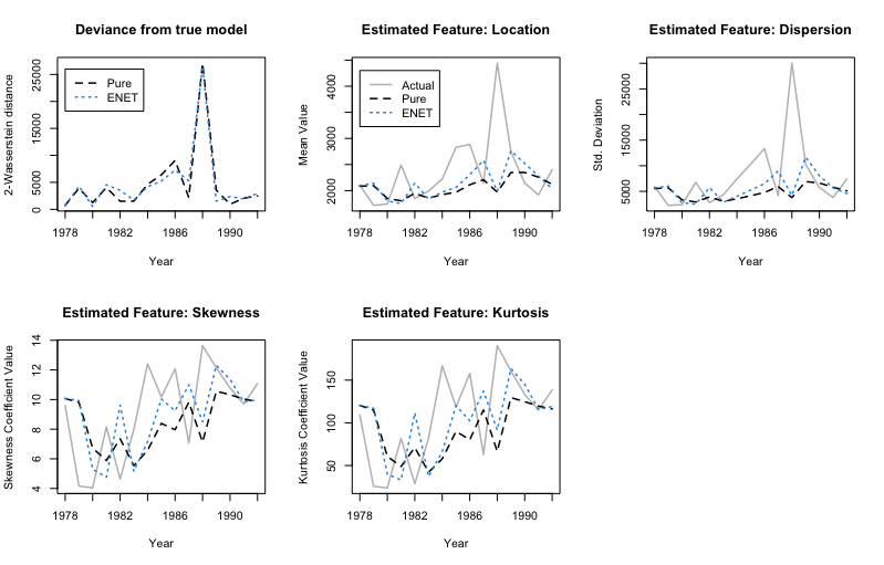
Figure 1: Illustration per year of the observed distributional characteristics (gray line) and the estimated ones by the pure barycenter (black dashed line) and the ENET barycenter (blue dot line).

The approximation of the actual (realized) claim size distribution by both the pure average model and the ENET-penalized average model appears to be at comparable levels, as illustrated in Figure 1 (upper panel, left plot). The estimation accuracy of the overall distribution seems to improve over the years, as the set ${\mathcal{M}}$ expands, with the notable exceptions of the extreme jumps in 1986 and 1988, where the observed distributions are markedly dissimilar compared to previous years (please see the descriptive statistics in Section E in the Appendix). Regarding the prediction of the mean tendency and variance, both averaging schemes deliver close estimates while ENET variant seems to capture slightly better increasing trends. However, when it comes to approximating higher-order distributional characteristics (such as skewness and kurtosis), the ENET variant appears more effective, as the pure averaging scheme tends to underestimate these features (lower panel of plots in Figure 1). Considering the pronounced heavy-tail behavior and the substantial heterogeneity among the involved distributions, both schemes achieve quite decent approximation of the actual model.

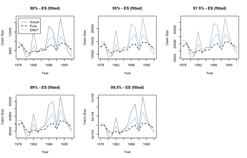
Figure 2: Illustration of the calibrated upper tail ES from the pure barycenter (black dashed line) and the ENET barycenter (blue dot line) averaging schemes.

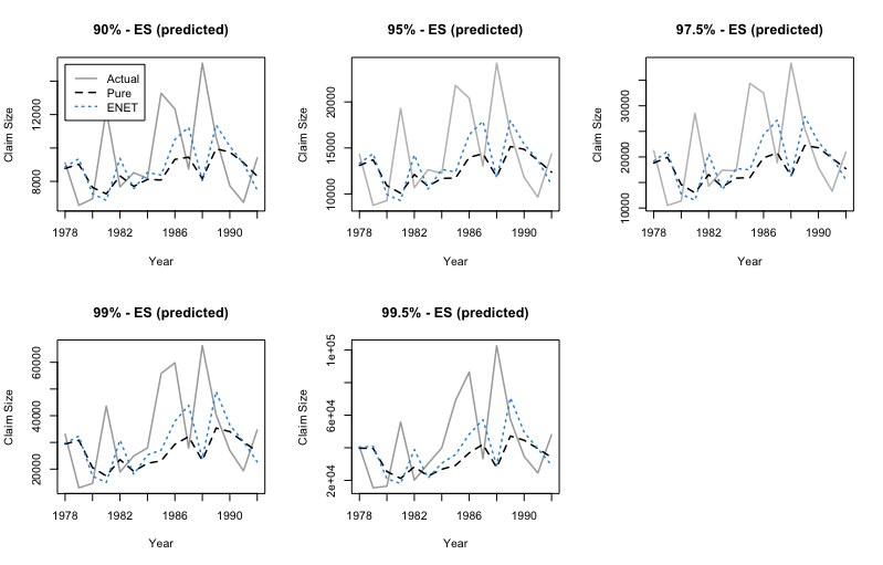
Figure 3: Illustration of the 1-year ahead predictions for the upper tail ES by the pure barycenter (black dashed line) and the ENET barycenter (blue dot line) averaging models.

To assess the risk taking into account also sgnificant heavy tail behavior (tail risk), we consider the Expected Shortfall (ES) as a more appropriate risk measure. ES is determined for any level $p\in(0,1)$ through the relation

$$\mbox{ES}_{p}=\frac{1}{1-p}\int_{p}^{1}\mbox{VaR}_{s}ds$$

where $\mbox{VaR}_{p}$ denotes the standard Value at Risk (VaR) which coincides with the $p$-th quantile of the loss variable for continuous distributions. In Figure 2 we illustrate per year the ES approximation when fitting the relevant averaging models (fitting phase), while in Figure (3) is illustrated the 1-year ahead prediction of ES through the proposed averaging schemes (in Section F in the Appendix are included the respective figures for VaR).

It is evident that as more data become available, both schemes demonstrate improved approximation performance. However, the ENET variant generally displays superior approximation performance in fitting stages, as illustrated in Figure 2, since it better captures the ES patterns at all levels. Moreover, concerning the 1-year ahead prediction of ES, the ENET variant again stays closer to the realized ES at almost all cases, improving potential underestimations of the actual risk as provided by the pure averaging model, owing to its ability to better approximate the distributional shape features. Note that the observed biases on the prediction task is largely a consequence of the extreme, non-systematically occurring claim sizes. Although, the studied problem is by nature a quite challenging one, the ability of both schemes to replicate the trend of the upper parts of the loss distribution is remarkable, especially given that the averaging procedures were designed to capture the entire distribution rather than focusing solely on the right tail. Clearly, such approaches could serve as a foundation for the development of more refined local schemes specifically targeting heavy-tail behavior.

Both averaging schemes benefit from an expanding prior model basis as more data become available, and this is clearly reflected in Tables 3 and 4, which present the optimal weights determined for each model during the fitting stage. Specifically, the displayed weights correspond to the solutions obtained from problem (16). Notably, the effect of the ENET penalization becomes more evident as the size of the prior set $\mathcal{M}_{j-1}$ grows: the ENET-averaging model effectively reduces the number of active components (i.e. models assigned non-zero weights), promoting a more parsimonious and selective aggregation.

Validation	Weighting of the available empirical evidence
Year	1972	1973	1974	1975	1976	1977	1978	1979	1980	1981	1982	1983	1984	1985	1986	1987	1988	1989	1990
1977	0.10	.	0.21	0.39	0.29
1978	0.08	.	0.24	0.03	0.10	0.54
1979	0.35	0.19	.	0.23	0.01	.	0.23
1980	0.12	0.15	.	0.08	.	0.21	.	0.44
1981	0.03	.	.	.	.	0.43	0.05	.	0.49
1982	0.19	.	0.01	.	.	.	0.10	0.39	0.14	0.16
1983	0.11	.	.	0.15	0.05	0.06	0.04	0.20	.	0.12	0.28
1984	0.01	0.02	0.03	.	0.10	0.11	0.03	0.25	.	.	.	0.45
1985	.	.	0.09	0.20	0.06	.	0.09	0.07	.	0.28	0.18	.	0.02
1986	0.07	.	.	0.17	0.08	.	0.11	.	.	0.17	0.09	.	0.20	0.11
1987	.	.	.	0.01	.	.	0.12	0.25	.	.	0.35	.	0.10	0.09	0.08
1988	.	.	0.02	.	0.22	0.16	.	.	.	0.15	.	0.22	0.03	0.07	.	0.14
1989	.	0.01	.	0.10	0.11	.	.	.	.	.	0.11	.	0.17	0.24	.	0.21	0.05
1990	.	.	.	0.02	0.11	.	.	.	.	.	0.15	0.12	0.13	0.04	.	0.20	.	0.23
1991	.	.	0.08	.	0.02	0.03	.	.	.	.	0.08	0.14	0.24	.	.	0.12	.	0.01	0.27

Table 3: Optimal weights for the pure Wasserstein barycenter model averaging scheme.

Validation	Weighting of the available empirical evidence
Year	1972	1973	1974	1975	1976	1977	1978	1979	1980	1981	1982	1983	1984	1985	1986	1987	1988	1989	1990
1977	.	.	0.19	0.57	0.24
1978	.	.	0.20	0.01	.	0.79
1979	0.64	0.31	.	0.05	.	.	.
1980	0.21	0.21	.	0.06	.	.	.	0.52
1981	.	.	.	.	.	0.84	0.00	0.00	0.16
1982	0.26	.	.	.	.	.	.	0.52	0.04	0.18
1983	0.02	.	.	0.29	.	0.02	0.21	.	.	0.10	0.36
1984	.	.	.	.	0.25	.	0.32	0.20	.	.	.	0.24
1985	.	.	0.03	0.05	0.05	.	0.43	.	.	0.43	.	.	.
1986	.	.	.	.	.	.	.	.	.	0.09	.	.	0.32	0.60
1987	.	.	.	.	.	.	0.21	0.02	.	.	0.41	.	0.36	.	.
1988	.	.	.	.	0.42	0.07	.	.	.	0.06	.	.	.	0.26	0.20	.
1989	.	.	.	.	0.11	.	.	.	.	.	.	.	0.18	0.09	.	0.42	0.20
1990	.	.	.	.	.	.	.	.	.	.	.	.	0.22	.	.	0.53	.	0.25
1991	.	.	.	.	.	.	.	0.24	.	.	.	.	0.24	.	.	.	.	.	0.52

Table 4: Optimal weights for the ENET Wasserstein barycenter model averaging scheme.

4 Conclusions & Discussion

In this work we addressed the problem of model averaging in the space of probability distributions, leveraging Wasserstein barycenters and regularization techniques from the elastic net family. The proposed approach enables a unified treatment of model averaging and selection in complex, non-Euclidean model spaces, extending traditional penalization methods to the setting of measure-valued data. A key theoretical contribution is the establishment of strong consistency results via the variational framework of $\Gamma$-convergence, ensuring asymptotically valid estimation as data accumulates.

Also, through comprehensive simulations as well as a real-data application, we demonstrate the empirical benefits, practical relevance, and effectiveness of our approach across diverse distributional settings. The results affirm that regularization is not merely a computational device but a statistically essential component in learning and aggregating probability models within the Wasserstein framework. Future directions include localized aggregation methods for improved tail behavior approximation and extensions to multivariate settings, where optimal aggregation may require novel numerical and regularization strategies.

Appendix

In Appendix, we provide detailed technical support for the main text. Specifically, we present complete analytical proofs for Theorem 2 and Proposition 1, which establish the theoretical foundations of our proposed methodology. Theorem 2 concerns the variational consistency of the elastic net-regularized Wasserstein barycenter estimator via $\Gamma$-convergence, while Proposition 1 characterizes the sparsity-inducing properties of the estimator through the proximal operator framework.

In addition, we report tabulated numerical results corresponding to the two simulation experiments discussed in the main paper. Experiment I is based on Normal distributions, and Experiment II on Weibull distributions with varying shape parameters. For each setting, we report both the Wasserstein-2 distances achieved by different penalization schemes (LASSO, Ridge, and Elastic Net), and the corresponding weight deviation metrics and optimal regularization parameters. Finally, we include additional visualizations of fitted and predicted Value at Risk (VaR) curves to illustrate the practical relevance of the method in risk estimation applications.

Appendix A Proof of Theorem 2

Proof.

(i) Since the sequence $\{{\bf S_{n}}\}$ consists of positive definite matrices for any $n$ (by construction), the mappings ${\bf w}\mapsto J_{n}({\bf w},\cdot)$ are convex functions for any $n$ and therefore it holds that $J_{n}({\bf w},\cdot)\to J({\bf w})$ pointwise in $S_{J}\subset{\mathbb{R}}^{J}$. Note that both $J_{n},J$ can be decomposed as

$$J_{n}({\bf w})=J_{0,n}({\bf w})+G({\bf w}),\,\,\,J({\bf w})=J_{0}({\bf w})+G({\bf w})$$

where $G(\cdot):=\lambda\Psi(\cdot)$ is a continuous function by assumption (P1). By the properties of $\Gamma$-limits (please see Prop. 6.21 in Dal Maso (2012)), if $J_{0,n}\xrightarrow{\Gamma}J_{0,n}$ then $(J_{0,n}+G)\xrightarrow{\Gamma}(J_{0}+G)$, too. We employ the pointwise convergence of $\{J_{n}\}$ alongside to the convexity and equi-boundness properties to show the $\Gamma$-convergence of $J_{n}$ to $J$. In the following two steps, we retrieve the side $\Gamma$-limits for $J_{n}$.

Step 1. The LII inequality is obtained as

$$J({\bf w}) = \lim_{n}J_{n}({\bf w})=\liminf_{n}J_{n}({\bf w})=\liminf_{n}\left(J_{n}({\bf w})-J_{n}({\bf w}_{n})+J_{n}({\bf w}_{n})\right)$$ (17)

$$\leq \liminf_{n}\left(|J_{n}({\bf w})-J_{n}({\bf w}_{n})|+J_{n}({\bf w}_{n})\right)=\liminf_{n}|J_{n}({\bf w}_{n})-J_{n}({\bf w})|+\liminf_{n}J_{n}({\bf w}_{n})$$

$$= \liminf_{n}J_{n}({\bf w}_{n})$$

This holds for all sequences ${\bf w}_{n}\to{\bf w}$, and consequently for the infimum of the random functionals over the set of all such sequences, which corresponds to the $\Gamma$-$\liminf_{n}J_{n}$.

Step 2. Now we prove the LSI. Taking the infimum over all ${\bf w}_{n}\to{\bf w}$ in (17) we get:

$$J({\bf w}) \leq \inf\{\liminf_{n}J_{n}({\bf w}_{n})\,\,|\,\,{\bf w}_{n}\to{\bf w}\}=:(\Gamma-\liminf J_{n})({\bf w})$$ (18)

$$\leq (\Gamma-\limsup_{n}J_{n})({\bf w})=\inf\{\limsup_{n}J_{n}({\bf w}_{n})\,\,|\,\,{\bf w}_{n}\to{\bf w}\}$$

$$\leq \limsup_{n}J_{n}({\bf w})=J({\bf w})$$

So, (17) and (18) yield that

$$J({\bf w})\leq(\Gamma-\liminf_{n}J_{n})({\bf w})\leq(\Gamma-\limsup_{n}J_{n})({\bf w})\leq J({\bf w})$$

which results that $\Gamma-\lim_{n}J({\bf w})=J({\bf w})$. The above arguments shows that fixing $\omega\in\Omega$, we get that $J_{n}(\cdot,\omega)\xrightarrow{\Gamma}J(\cdot)$ for $J_{n},J$ as above. Thus, since the a.s. refers to the set of $A\subset\Omega$ for which the convergence does not hold, and since this set is a nullset $(P(A)=0)$ the $\Gamma$-convergence holds almost surely.

(ii) It holds that for all $n\in{\mathbb{N}}$ and $\omega\in\Omega$ that $J_{n}({\bf w},\omega)\geq\lambda\Psi({\bf w})=:G({\bf w})$ with $G(\cdot)$ being a deterministic (independent of $\omega$), continuous and coercive function. Hence, by Definition 2 in the manuscript (or Proposition 7.7 in Dal Maso (2012)) the sequence $\{J_{n}\}$ is equi-coercive.

(iii) Let us consider the space $\Omega^{\prime}\subset\Omega$ where $\Omega^{\prime}:=\Omega\setminus A$ with $A:=\{\omega\in\Omega\,\,:\,\,J_{n}(\cdot,\omega)\not\xrightarrow{\Gamma}J(\cdot)\}$ and $P(A)=0$. Therefore, $\Omega^{\prime}$ is a full measure space, i.e. $P(\Omega^{\prime})=1$. For any $\omega\in\Omega^{\prime}$ then it holds that $J_{n}(\cdot,\omega)\xrightarrow{\Gamma}J(\cdot)$, i.e. this holds almost surely in $\Omega$. Due to the equicoercivity property of $\{J_{n}\}$, there exists a compact and nonempty set $K\subset{\mathbb{R}}^{J}$ for which

$$\inf_{{\bf w}\in{\mathbb{R}}^{J}}J_{n}({\bf w})=\inf_{{\bf w}\in K}J_{n}({\bf w}),\,\,\,\forall n\in\mathbb{N}.$$

In fact the set $K$ in our case is identified by the set $S_{J}$. Now, we may provide our main result in three steps.

Step 1. First, we show that $\inf_{{\bf w}\in{\mathbb{R}}^{J}}J({\bf w})\leq\liminf_{n}\left(\inf_{{\bf w}\in{\mathbb{R}}^{J}}J_{n}({\bf w})\right)$. Since $\{J_{n}\}$ is lower semicontinuous and the set $S_{J}$ compact, for all $n\in{\mathbb{N}}$ there exists a sequence $\{{\bf w}_{n}^{*}\}\in S_{J}$ such that $\inf_{{\bf w}\in S_{J}}J_{n}({\bf w})=J_{n}({\bf w}_{n}^{*})$ (due to equi-coercivity). We want to compare $\liminf_{n}\inf_{S_{J}}J_{n}({\bf w})$ and $\liminf_{n}J_{n}({\bf w}_{n}^{*})$. We consider a subsequence $\{{\bf w}^{*}_{n_{k}}\}\subset\{{\bf w}_{n}^{*}\}\subset S_{J}$ such that $\liminf_{n}J_{n}({\bf w}_{n}^{*})=\lim_{k}J_{n_{k}}({\bf w}^{*}_{n_{k}})$. Since $S_{J}$ is compact, there exists $\{{\bf w}^{*}_{n_{k_{\ell}}}\}\subset\{{\bf w}^{*}_{n_{k}}\}\subset\{{\bf w}_{n}^{*}\}\subset S_{J}$ and ${\bf w}^{*}\in S_{J}$ such that ${\bf w}^{*}_{n_{k_{\ell}}}\to{\bf w}^{*}$. Let us define

$$\widetilde{{\bf w}}_{n}:=\left\{\begin{array}[]{ll}{\bf w}^{*}_{n_{k_{\ell}}},&\mbox{for }n\leq n_{k_{\ell}}\\ {\bf w}^{*},&\mbox{elsewhere}.\end{array}\right.$$

Then, we have

$$\inf_{{\bf w}\in S_{J}}J({\bf w}) \leq J({\bf w}^{*})\leq\liminf_{n}J_{n}(\widetilde{{\bf w}}_{n})\leq\liminf_{\ell}J_{n_{k_{\ell}}}(\widetilde{{\bf w}}_{n_{k_{\ell}}})=\liminf_{\ell}J_{n_{k_{\ell}}}({\bf w}^{*}_{n_{k_{\ell}}})$$ (20)

$$= \liminf_{n}\left(\inf_{{\bf w}\in S_{J}}J_{n}({\bf w})\right).$$

Step 2. By definition of $\inf$ for all $\epsilon>0$ there exists ${\bf w}_{\epsilon}\in{\mathbb{R}}^{J}$ such that $J({\bf w}_{\epsilon})<\inf_{{\mathbb{R}}^{J}}J({\bf w})+\epsilon$. Since $J$ is a $\Gamma$-limit, we use a recovery sequence $\{{\bf w}_{\epsilon,n}\}_{n}$ converging to ${\bf w}_{\epsilon}$ for which $\limsup_{n}\left(\inf_{{\mathbb{R}}^{J}}J_{n}({\bf w})\right)\leq\limsup_{n}J_{n}({\bf w}_{\epsilon,n})\leq J({\bf w}_{\epsilon})<\inf_{{\mathbb{R}}^{J}}J({\bf w})+\epsilon$ where for $\epsilon\to 0$ and using the equi-coercivity of $J_{n}$ we get

$$\limsup_{n}\left(\inf_{S_{J}}J_{n}({\bf w})\right)\leq\inf_{S_{J}}J({\bf w}).$$ (21)

Step 3. By (20), (21) and equi-coercivity property of $\{J_{n}\}$, we get

$$\inf_{{\bf w}\in{\mathbb{R}}^{J}}J({\bf w}) \leq \min_{{\bf w}\in S_{J}}J({\bf w})\leq\liminf_{n}\left(\inf_{{\bf w}\in S_{J}}J_{n}({\bf w})\right)=\liminf_{n}\left(\inf_{{\bf w}\in{\mathbb{R}}^{J}}J_{n}({\bf w})\right)$$

$$\leq \limsup_{n}\left(\inf_{{\bf w}\in{\mathbb{R}}^{J}}J_{n}({\bf w})\right)\leq\inf_{{\bf w}\in{\mathbb{R}}^{J}}J({\bf w}).$$

Hence, it holds that $\min_{{\bf w}\in{\mathbb{R}}^{J}}J({\bf w})=\lim_{n}\left(\inf_{{\bf w}\in{\mathbb{R}}^{J}}J_{n}({\bf w})\right)$. Now consider $\{{\bf w}_{n}\}$ as a sequence of minimizers for $\{J_{n}\}$, and ${\bf w}^{*}$ a cluster point of $\{{\bf w}_{n}\}$. Then, it holds that $J_{n}({\bf w}_{n})=\inf_{{\bf w}\in{\mathbb{R}}^{J}}J_{n}({\bf w})=\inf_{{\bf w}\in S_{J}}J_{n}({\bf w})$. Using the liminf ineq we get

$$J({\bf w}^{*}) \leq \liminf_{n}J_{n}({\bf w}_{n})=\liminf_{n}\left(\inf_{{\bf w}\in S_{J}}J_{n}({\bf w})\right)=\liminf_{n}\left(\inf_{{\bf w}\in{\mathbb{R}}^{J}}J_{n}({\bf w})\right)$$

$$\leq \limsup_{n}\left(\inf_{{\bf w}\in{\mathbb{R}}^{J}}J_{n}({\bf w})\right)\leq\inf_{{\bf w}\in{\mathbb{R}}^{J}}J({\bf w})$$

i.e. we conclude that ${\bf w}^{*}$ is a minimizer for $J$. ∎

Appendix B Proof of Proposition 1

Proof.

The function to be optimized has two contributions, a smooth part and a non smooth one. We denote these by

$$f_{1}({\bf w})=\frac{1}{2}\langle g({\bf w})-\hat{g}_{0},g({\bf w})-\hat{g}_{0}\rangle+\lambda\frac{1-\alpha}{2}\|{\bf w}\|_{2}^{2},$$

$$f_{2}({\bf w})=\lambda\alpha\|{\bf w}\|_{1}$$

The first order conditions for a solution ${\bf w}^{*}$, without constraining $w$ on the unit simplex, are

$$0\in\partial(f_{1}+f_{2})({\bf w}^{*})=\partial f_{1}({\bf w}^{*})+\partial f_{2}({\bf w}^{*})$$ (22)

where $\partial\varphi$ is the subdifferential of the function $\phi$ and we also used subdifferential calculus and the continuity of the functions $f_{1}$ and $f_{2}$. We now rearrange (22) in terms of the auxiliary variable ${\bf z}$ as

$$\frac{1}{\gamma}({\bf w}^{*}-{\bf z})+\frac{1}{\gamma}({\bf z}-{\bf w}^{*})\in Df_{1}({\bf w}^{*})+\partial f_{2}({\bf w}^{*}),$$

which is broken up as

$$\left\{\begin{array}[]{cc}&{\bf w}^{*}-{\bf z}=\gamma Df_{1}({\bf w}^{*}),\\ &{\bf z}-{\bf w}^{*}\in\gamma\partial f_{2}({\bf w}^{*})\end{array}\right.\,\,\,\Longleftrightarrow\,\,\left\{\begin{array}[]{cc}&{\bf z}={\bf w}^{*}-\gamma Df_{1}({\bf w}^{*}),\\ &{\bf w}^{*}=(I+\gamma\partial f_{2})^{-1}({\bf z})=\mbox{Prox}_{\gamma,f_{2}}({\bf z})\end{array}\right.$$ (23)

where the proximal operator related to the non smooth function $f_{2}$ is defined by

$$\mbox{Prox}_{\gamma,f_{2}}({\bf z}):=(I+\gamma\partial f_{2})^{-1}({\bf z})=\arg\min_{{\bf y}}\bigg{(}f_{2}({\bf y})+\frac{1}{2\gamma}\|{\bf y}-{\bf z}\|_{2}^{2}\bigg{)}$$

for $\gamma>0$. Note that eventhough $\partial f_{2}$ is a multivalued operator, the proximal operator is single valued. A closely related notion is the Moreau-Yosida approximation of $f_{2}$, defined by

$$f_{2,\gamma}({\bf z})=\min_{{\bf y}}\bigg{(}f_{2}({\bf y})+\frac{1}{2\gamma}\|{\bf y}-{\bf z}\|_{2}^{2}\bigg{)},$$

which provides a smooth approximation to the non smooth function $f_{2}$, sharing the same minimizers (Kravvaritis and Yannacopoulos, 2020). The sparsity effects of our estimator comes from the second equation in (23). Indeed, one can directly calculate $\mbox{Prox}_{\gamma,f_{2}}({\bf z})$ if $f_{2}({\bf z})=\|{\bf z}\|_{1}=\sum_{j=1}^{J}|z_{j}|$, in terms of $\mbox{Prox}_{\gamma,f_{2}}({\bf z})=(v_{1},\ldots,v_{J})^{\prime}$ where

$$v_{j}=\left\{\begin{array}[]{rc}z_{j}+\gamma\lambda\alpha,&z_{j}<-\gamma\lambda\alpha\\ 0,&-\gamma\lambda\alpha\leq z_{j}\leq\gamma\lambda\alpha\\ z_{j}-\gamma\lambda\alpha,&z_{j}>\gamma\lambda\alpha\end{array}\right.$$ (24)

On the other hand, we can directly calculate $Df_{1}({\bf w})=(u_{1},\ldots,u_{J})^{\prime}$, where

$$u_{j}=\frac{\partial f_{2}}{\partial w_{j}}({\bf w})=\int_{0}^{1}g_{j}(s)\left(\sum_{k=1}^{J}w_{k}g_{k}(s)-\hat{g}_{0}(s)\right)ds+\lambda(1-\alpha)w_{j}=:C_{j}+\lambda(1-\alpha)w_{j},$$

and the first term $C_{j}$ can be interpreted as the correlation of the quantile $g_{j}(\cdot)$ with the “error” of the model $e(s):=\sum_{k=1}^{J}w_{k}g_{k}(s)-\hat{g}_{0}(s)$. Hence, combining the form of the proximal operator and the second equation in (23) we see that the coefficients $w_{j}=0$ for these $j$ for which

$$|z_{j}|=|(1-\lambda\gamma(1-\alpha)w_{j}-\gamma C_{j}|=\gamma|C_{j}|\leq\gamma\lambda\alpha.$$

An alternative way of looking at the sparsity effect is starting from the first order condition (22) directly and noting that $\partial f_{2}({\bf w})=\{(p_{1},\ldots,p_{J})\,\,:\,\,(-\lambda\alpha){\bf 1}_{w_{j}<0}+v_{j}{\bf 1}_{w_{j}=0}+(\lambda\alpha){\bf 1}_{w_{j}>0},\,\,\,v_{j}\in[-\lambda\alpha,\lambda\alpha]\}$. The first order condition then yields $-Df_{1}({\bf w}^{*})\in\partial f_{2}({\bf w}^{*})$, which by the above implies that $w_{j}^{*}=0$ if and only if $C_{j}+\lambda(1-\alpha)w_{j}^{*}=C_{j}=v_{j}\in[-\lambda\alpha,\lambda\alpha]$, hence, $|C_{j}|<\lambda\alpha$, which is equivalent to our previous result. We then project on the positive cone of ${\mathbb{R}}^{J}$, an operation that preserves the sparsity effect, and then we normalize the resulting weights dividing by the sum of all weights ensuring that all sum up to one (an operation that still preserves the sparsity). ∎

Appendix C Tabulated results from Numerical Experiment I - Normal distribution case

			Penalization Term
		Pure Barycenter		LASSO		Ridge		Elastic Net
$J$	$n$	Mean	s.e.	Mean	s.e.	Mean	s.e.	Mean	s.e.
5	$100$	0.1539	$17.12\cdot 10^{-4}$	0.1494	$16.47\cdot 10^{-4}$	0.1502	$16.55\cdot 10^{-4}$	**0.1490	$16.30\cdot 10^{-4}$
	$200$	0.1126	$12.54\cdot 10^{-4}$	0.1101	$12.31\cdot 10^{-4}$	0.1104	$12.24\cdot 10^{-4}$	**0.1097	$12.16\cdot 10^{-4}$
	$500$	0.0754	$8.02\cdot 10^{-4}$	0.0739	$7.76\cdot 10^{-4}$	0.0747	$7.89\cdot 10^{-4}$	**0.0738	$7.74\cdot 10^{-4}$
10	$100$	0.1451	$16.46\cdot 10^{-4}$	**0.1318	$14.90\cdot 10^{-4}$	0.1372	$15.54\cdot 10^{-4}$	0.1334	$15.05\cdot 10^{-4}$
	$200$	0.1067	$11.64\cdot 10^{-4}$	**0.0979	$10.76\cdot 10^{-4}$	0.1022	$11.12\cdot 10^{-4}$	0.0992	$10.83\cdot 10^{-4}$
	$500$	0.0707	$7.26\cdot 10^{-4}$	**0.0658	$6.73\cdot 10^{-4}$	0.0693	$7.00\cdot 10^{-4}$	0.0667	$6.79\cdot 10^{-4}$
20	$100$	0.1324	$18.42\cdot 10^{-4}$	**0.1048	$16.67\cdot 10^{-4}$	0.1138	$16.44\cdot 10^{-4}$	0.1071	$15.97\cdot 10^{-4}$
	$200$	0.0955	$15.16\cdot 10^{-4}$	**0.0776	$13.44\cdot 10^{-4}$	0.0846	$13.82\cdot 10^{-4}$	0.0796	$13.34\cdot 10^{-4}$
	$500$	0.0691	$7.54\cdot 10^{-4}$	**0.0590	$6.74\cdot 10^{-4}$	0.0653	$7.10\cdot 10^{-4}$	0.0610	$6.86\cdot 10^{-4}$

Table 5: Average Wasserstein distance of the aggregate model from the empirical model for the Normal distribution (N(0,1)) case. Evaluation is performed over a set of $B=1000$ simulations.

		Penalization Term
		LASSO			Ridge			Elastic Net
$J$	$n$	${\mathbb{E}}[\|\Delta{\bf w}\|]$	$\sigma(\|\Delta{\bf w}\|)$	$\lambda$	${\mathbb{E}}[\|\Delta{\bf w}\|]$	$\sigma(\|\Delta{\bf w}\|)$	$\lambda$	${\mathbb{E}}[\|\Delta{\bf w}\|]$	$\sigma(\|\Delta{\bf w}\|)$	$\lambda$	$\alpha$
5	$100$	0.1725	0.0049	3.7623	0.1157	0.0040	0.2710	0.1766	0.0041	1.2075	0.8137
	$200$	0.1417	0.0046	3.2810	0.0989	0.0039	0.1965	0.1454	0.0037	0.5114	0.8313
	$500$	0.1279	0.0046	2.7082	0.0659	0.0041	0.1341	0.1295	0.0039	0.2123	0.8024
10	$100$	0.3155	0.0052	3.6221	0.1724	0.0034	0.2045	0.2450	0.0031	1.5045	0.8592
	$200$	0.2949	0.0052	2.9832	0.1567	0.0035	0.0925	0.2205	0.0031	0.4192	0.8740
	$500$	0.2655	0.0053	2.4683	0.0981	0.0039	0.0255	0.1943	0.0030	0.0968	0.8644
20	$100$	0.3787	0.1171	3.7591	0.2119	0.0744	0.2119	0.2614	0.0584	2.0517	0.8788
	$200$	0.3437	0.1326	2.9752	0.1943	0.0759	0.0671	0.2397	0.0596	0.4979	0.8923
	$500$	0.3696	0.1579	2.3323	0.1628	0.0978	0.0234	0.2321	0.0655	0.0790	0.8888

Table 6: Weight allocation difference from each penalization method comparing to the pure barycenter optimal weights (mean value and std. deviation of the euclidean norm) and the optimal penalization parameters (mean values)

Appendix D Tabulated results from Numerical Experiment II - Weibull distribution case

				Penalization Term
			Pure Barycenter		LASSO		Ridge		Elastic Net
$\alpha$	$J$	$n$	Mean	s.e.	Mean	s.e.	Mean	s.e.	Mean	s.e
$=1$	5	$100$	0.2342	$4.07\cdot 10^{-3}$	0.2159	$3.92\cdot 10^{-3}$	0.1830	$3.18\cdot 10^{-3}$	**0.1801	$3.14\cdot 10^{-3}$
		$500$	0.1803	$3.26\cdot 10^{-3}$	0.1590	$2.99\cdot 10^{-3}$	0.1257	$2.42\cdot 10^{-3}$	**0.1213	$2.40\cdot 10^{-3}$
	10	$100$	0.2078	$3.45\cdot 10^{-3}$	0.1709	$3.17\cdot 10^{-3}$	0.1527	$2.52\cdot 10^{-3}$	**0.1468	$2.51\cdot 10^{-3}$
		$500$	0.1449	$2.44\cdot 10^{-3}$	0.1166	$2.24\cdot 10^{-3}$	0.0948	$1.54\cdot 10^{-3}$	**0.0867	$1.51\cdot 10^{-3}$
	20	$100$	0.1961	$4.63\cdot 10^{-3}$	0.1429	$4.17\cdot 10^{-3}$	0.1344	$3.13\cdot 10^{-3}$	**0.1251	$3.09\cdot 10^{-3}$
		$500$	0.1286	$2.85\cdot 10^{-3}$	0.0916	$2.47\cdot 10^{-3}$	0.0859	$1.88\cdot 10^{-3}$	**0.0758	$1.81\cdot 10^{-3}$
$>1$	5	$100$	0.1666	$2.94\cdot 10^{-3}$	0.1528	$2.84\cdot 10^{-3}$	0.1304	$2.36\cdot 10^{-3}$	**0.1284	$2.35\cdot 10^{-3}$
		$500$	0.1406	$2.38\cdot 10^{-3}$	0.1253	$2.33\cdot 10^{-3}$	0.0977	$1.82\cdot 10^{-3}$	**0.0929	$1.84\cdot 10^{-3}$
	10	$100$	0.1482	$2.42\cdot 10^{-3}$	0.1212	$2.32\cdot 10^{-3}$	0.1061	$1.75\cdot 10^{-3}$	**0.1012	$1.74\cdot 10^{-3}$
		$500$	0.1139	$1.93\cdot 10^{-3}$	0.0920	$1.83\cdot 10^{-3}$	0.0722	$1.21\cdot 10^{-3}$	**0.0660	$1.19\cdot 10^{-3}$
	20	$100$	0.1338	$3.11\cdot 10^{-3}$	0.1005	$2.89\cdot 10^{-3}$	0.0979	$2.24\cdot 10^{-3}$	**0.0906	$2.28\cdot 10^{-3}$
		$500$	0.0973	$2.20\cdot 10^{-3}$	0.0733	$2.09\cdot 10^{-3}$	0.0637	$1.39\cdot 10^{-3}$	**0.0562	$1.32\cdot 10^{-3}$
$<1$	5	$100$	0.5629	$11.53\cdot 10^{-3}$	0.4916	$10.57\cdot 10^{-3}$	0.4432	$10.35\cdot 10^{-3}$	**0.4376	$10.26\cdot 10^{-3}$
		$500$	0.4325	$11.24\cdot 10^{-3}$	0.3406	$9.92\cdot 10^{-3}$	0.3117	$10.38\cdot 10^{-3}$	**0.2999	$9.92\cdot 10^{-3}$
	10	$100$	0.5022	$9.85\cdot 10^{-3}$	0.3773	$7.72\cdot 10^{-3}$	0.3579	$7.64\cdot 10^{-3}$	**0.3431	$7.32\cdot 10^{-3}$
		$500$	0.4065	$7.37\cdot 10^{-3}$	0.2644	$5.09\cdot 10^{-3}$	0.2618	$5.39\cdot 10^{-3}$	**0.2399	$5.06\cdot 10^{-3}$
	20	$100$	0.5030	$11.95\cdot 10^{-3}$	0.3707	$10.19\cdot 10^{-3}$	0.3849	$10.01\cdot 10^{-3}$	**0.3662	$9.91\cdot 10^{-3}$
		$500$	0.3444	$8.12\cdot 10^{-3}$	**0.2200	$5.25\cdot 10^{-3}$	0.2649	$6.79\cdot 10^{-3}$	0.2340	$6.34\cdot 10^{-3}$

Table 7: Average Wasserstein distance of the aggregate model from the empirical model for the Weibull distribution case with parameters $\alpha$ (shape) and $\kappa$ (scale). Evaluation is performed over a set of $B=1000$ simulations.

			Penalization Term
			LASSO			Ridge			Elastic Net
$\alpha$	$J$	$n$	${\mathbb{E}}[\|\Delta{\bf w}\|]$	$\sigma(\|\Delta{\bf w}\|)$	${\mathbb{E}}[\lambda]$	${\mathbb{E}}[\|\Delta{\bf w}\|]$	$\sigma(\|\Delta{\bf w}\|)$	${\mathbb{E}}[\lambda]$	${\mathbb{E}}[\|\Delta{\bf w}\|]$	$\sigma(\|\Delta{\bf w}\|)$	${\mathbb{E}}[\lambda]$	${\mathbb{E}}[\alpha]$
$=1$	5	$100$	0.1093	0.1437	2.2688	0.2299	0.1964	1.0029	0.2474	0.1876	1.8524	0.6693
		$500$	0.1073	0.1479	1.8713	0.2514	0.2041	0.5784	0.2576	0.1873	0.8831	0.7155
	10	$100$	0.1959	0.1624	1.8762	0.2242	0.1625	0.6192	0.2520	0.1437	1.4911	0.7327
		$500$	0.1726	0.1655	1.4321	0.2363	0.1671	0.3657	0.2471	0.1460	0.7046	0.7529
	20	$100$	0.3055	0.1617	2.1124	0.1882	0.1291	0.6952	0.2449	0.1052	1.9225	0.7392
		$500$	0.2322	0.1715	1.2619	1.8847	0.1236	0.3051	0.2112	0.1095	0.6382	0.7596
$>1$	5	$100$	0.1018	0.1359	2.2644	0.2232	0.1935	0.7870	0.2387	0.1839	1.5251	0.7070
		$500$	0.1053	0.1444	1.9627	0.2741	0.2058	0.5658	0.2733	0.1859	0.8175	0.6917
	10	$100$	0.2112	0.1737	1.8602	0.2189	0.1559	0.8414	0.2533	0.1399	1.8461	0.7099
		$500$	0.1671	0.1615	1.5137	0.2529	0.1658	0.3221	0.2532	0.1498	0.5951	0.7444
	20	$100$	0.2781	0.1616	1.8942	0.1754	0.1346	0.5536	0.2328	0.1049	1.5925	0.7757
		$500$	0.2184	0.1749	1.2377	0.1989	0.1166	0.2537	0.2144	0.1089	0.5453	0.7626
$<1$	5	$100$	0.1143	0.1602	2.7175	0.2153	0.2099	1.1724	0.2281	0.2060	2.3831	0.6638
		$500$	0.1343	0.1767	2.3230	0.2503	0.2235	0.3781	0.2494	0.2163	1.0440	0.7567
	10	$100$	0.1947	0.1819	2.1697	0.1897	0.1768	0.7784	0.2166	0.1733	1.8516	0.7002
		$500$	0.2198	0.1920	1.6676	0.2128	0.1960	0.2865	0.2250	0.1851	0.8121	0.7206
	20	$100$	0.2431	0.1883	1.9363	0.1311	0.1423	0.5072	0.1759	0.1455	1.3930	0.7154
		$500$	0.2508	0.2007	1.5678	0.1282	0.1461	0.1637	0.1612	0.1517	0.6377	0.6822

Table 8: Weight allocation difference from each penalization method comparing to the pure barycenter optimal weights (mean value and std. deviation of the euclidean norm) and the optimal penalization parameters (mean values)

Appendix E Descriptives for norfire dataset

							Quantiles
Year	n	Mean	St. Dev.	Skewness	Kurtosis	Median	75%	90%	95%	97.5%	99%	99.5%	Max
1972	97	1898.13	3370.22	5.60	40.36	916.00	1498.00	3393.40	6124.20	8784.80	14476.76	21265.88	28055.00
1973	109	1937.65	3046.80	5.72	45.12	830.00	1925.00	3915.80	6604.60	7671.50	9763.40	17844.50	27200.00
1974	110	2060.73	4506.96	6.85	56.99	892.00	1797.25	3028.50	6644.80	9768.17	18138.83	29225.61	41620.00
1975	142	2017.96	4883.35	8.33	83.34	911.00	1483.50	3255.40	6752.75	10287.85	15698.27	27669.08	52600.00
1976	207	2775.65	13776.09	13.54	190.26	949.00	1968.50	4136.20	6000.00	8123.45	14848.60	27599.21	196359.00
1977	235	2215.82	6831.18	11.22	147.76	931.00	1623.00	3099.20	6521.60	9771.90	23194.74	26390.11	95032.00
1978	299	2025.24	5378.86	10.01	125.63	938.00	1610.50	3112.20	5299.50	8392.90	24067.84	29515.16	75841.00
1979	355	1694.38	2157.35	3.94	23.53	930.00	1664.00	3637.60	5590.00	8447.90	9593.88	14192.04	19474.00
1980	373	1722.10	2303.09	3.88	22.24	870.00	1642.00	3859.40	6268.80	8576.20	11568.52	15193.52	19766.00
1981	429	2394.03	6140.30	8.07	82.37	932.00	1675.00	4046.40	7899.60	12645.90	28142.68	41519.76	77839.00
1982	428	1818.70	2684.63	4.57	28.39	921.50	1675.25	3991.60	5818.85	9720.55	16638.07	18970.14	23323.00
1983	407	1913.50	3785.04	7.78	84.36	925.00	1564.00	3530.00	5640.00	10327.25	18878.44	21788.07	51244.00
1984	557	2012.35	5456.64	14.63	259.91	1019.00	1750.00	3139.40	6080.40	8369.20	14874.84	17803.68	106495.00
1985	607	2552.70	8013.39	10.57	144.91	1000.00	1712.00	3500.00	7147.60	14923.65	28710.08	57669.09	135080.00
1986	647	2476.55	9695.04	13.92	234.95	985.00	1549.00	3399.80	6972.10	10643.80	28404.04	53701.36	188270.00
1987	767	2056.92	3643.71	6.79	60.56	1138.00	1853.00	3518.60	6035.00	9533.55	20007.18	28031.35	44926.00
1988	827	3176.15	17676.53	22.57	573.18	1176.00	2048.50	4550.20	7722.00	14192.85	26414.52	42175.88	465365.00
1989	718	2399.83	7094.13	14.38	258.99	1182.50	1995.50	3858.40	6188.05	12057.37	19532.40	32386.78	145156.00
1990	628	1973.52	4257.27	11.70	184.06	1150.00	1805.75	3247.30	4592.80	8434.45	16875.14	24877.47	78537.00
1991	624	1820.45	3019.42	9.57	129.21	1098.50	1909.00	3094.30	4774.70	8089.02	13307.89	15081.42	49692.00
1992	615	2184.24	5529.40	12.21	194.27	1060.00	1878.50	3548.00	6128.10	9898.65	15256.28	34694.89	102438.00

Table 9: Descriptive statistics for the fire losses data per year (claim sizes are expressed in Norwegian NKR).

Appendix F Value at Risk: fitted and predicted values

Figure 4: Illustration of the calibrations for the upper tail Value at Risk by the pure barycenter (black dashed line) and ENET barycenter (blue dot line) averaging models.

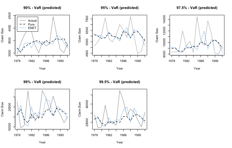
Figure 5: Illustration of the 1-year ahead predictions of the upper tail Value at Risk from the pure barycenter (black dashed line) and ENET barycenter (blue dot line) averaging models.

References

- Agueh and Carlier (2011) Agueh, M. and G. Carlier (2011). Barycenters in the Wasserstein space. SIAM Journal on Mathematical Analysis 43(2), 904–924.
- Avanzi et al. (2024) Avanzi, B., Y. Li, B. Wong, and A. Xian (2024). Ensemble distributional forecasting for insurance loss reserving. Scandinavian Actuarial Journal 2024(9), 971–1012.
- Bishop and Doucet (2021) Bishop, A. N. and A. Doucet (2021). Network consensus in the Wasserstein metric space of probability measures. SIAM Journal on Control and Optimization 59(5), 3261–3277.
- Chen et al. (2023) Chen, Y., Z. Lin, and H.-G. Müller (2023). Wasserstein regression. Journal of the American Statistical Association 118(542), 869–882.
- Christensen et al. (2018) Christensen, P., K. Gillingham, and W. Nordhaus (2018). Uncertainty in forecasts of long-run economic growth. Proceedings of the National Academy of Sciences 115(21), 5409–5414.
- Dal Maso (2012) Dal Maso, G. (2012). An introduction to -convergence, Volume 8. Springer Science & Business Media.
- Dubey and Müller (2019) Dubey, P. and H.-G. Müller (2019). Fréchet analysis of variance for random objects. Biometrika 106(4), 803–821.
- Dunlop et al. (2020) Dunlop, M. M., D. Slepčev, A. M. Stuart, and M. Thorpe (2020). Large data and zero noise limits of graph-based semi-supervised learning algorithms. Applied and Computational Harmonic Analysis 49(2), 655–697.
- Fan and Li (2001) Fan, J. and R. Li (2001). Variable selection via nonconcave penalized likelihood and its oracle properties. Journal of the American Statistical Association 96(456), 1348–1360.
- Fréchet (1948) Fréchet, M. (1948). Les éléments aléatoires de nature quelconque dans un espace distancié. In Annales de l’institut Henri Poincaré, Volume 10, pp. 215–310.
- Friederichs and Thorarinsdottir (2012) Friederichs, P. and T. L. Thorarinsdottir (2012). Forecast verification for extreme value distributions with an application to probabilistic peak wind prediction. Environmetrics 23(7), 579–594.
- Fronzek et al. (2022) Fronzek, S., Y. Honda, A. Ito, J. P. Nunes, N. Pirttioja, J. Räisänen, K. Takahashi, E. Terämä, M. Yoshikawa, and T. R. Carter (2022). Estimating impact likelihoods from probabilistic projections of climate and socio-economic change using impact response surfaces. Climate Risk Management 38, 100466.
- Gilat and Hill (1992) Gilat, D. and T. P. Hill (1992). One-sided refinements of the strong law of large numbers and the Glivenko-Cantelli theorem. The Annals of Probability, 1213–1221.
- Gneiting and Ranjan (2013) Gneiting, T. and R. Ranjan (2013). Combining predictive distributions. Electronic Journal of Statistics 7, 1747–1782.
- Hansen (2007) Hansen, B. E. (2007). Least squares model averaging. Econometrica 75(4), 1175–1189.
- Hartman and Groendyke (2013) Hartman, B. M. and C. Groendyke (2013). Model selection and averaging in financial risk management. North American Actuarial Journal 17(3), 216–228.
- Hoerl and Kennard (1970) Hoerl, A. E. and R. W. Kennard (1970). Ridge regression: Biased estimation for nonorthogonal problems. Technometrics 12(1), 55–67.
- Hong and Martin (2017) Hong, L. and R. Martin (2017). A flexible Bayesian nonparametric model for predicting future insurance claims. North American Actuarial Journal 21(2), 228–241.
- Hsiang et al. (2017) Hsiang, S., R. Kopp, A. Jina, J. Rising, M. Delgado, S. Mohan, D. J. Rasmussen, R. Muir-Wood, P. Wilson, M. Oppenheimer, et al. (2017). Estimating economic damage from climate change in the United States. Science 356(6345), 1362–1369.
- Kim and Pass (2017) Kim, Y.-H. and B. Pass (2017). Wasserstein barycenters over Riemannian manifolds. Advances in Mathematics 307, 640–683.
- Koundouri et al. (2024) Koundouri, P., G. I. Papayiannis, A. Vassilopoulos, and A. N. Yannacopoulos (2024). Probabilistic scenario-based assessment of national food security risks with application to Egypt and Ethiopia. Journal of the Royal Statistical Society Series A: Statistics in Society, qnae046.
- Kravvaritis and Yannacopoulos (2020) Kravvaritis, D. C. and A. N. Yannacopoulos (2020). Variational methods in nonlinear analysis: with applications in optimization and partial differential equations. Walter De Gruyter Gmbh & Co Kg.
- Kroshnin et al. (2021) Kroshnin, A., V. Spokoiny, and A. Suvorikova (2021). Statistical inference for Bures–Wasserstein barycenters. The Annals of Applied Probability 31(3), 1264–1298.
- Le Gouic and Loubes (2017) Le Gouic, T. and J.-M. Loubes (2017). Existence and consistency of Wasserstein barycenters. Probability Theory and Related Fields 168, 901–917.
- Lu and Su (2015) Lu, X. and L. Su (2015). Jackknife model averaging for quantile regressions. Journal of Econometrics 188(1), 40–58.
- Miljkovic and Grün (2021) Miljkovic, T. and B. Grün (2021). Using model averaging to determine suitable risk measure estimates. North American Actuarial Journal 25(4), 562–579.
- Moral-Benito (2015) Moral-Benito, E. (2015). Model averaging in economics: An overview. Journal of Economic Surveys 29(1), 46–75.
- Muis et al. (2015) Muis, S., B. Güneralp, B. Jongman, J. C. Aerts, and P. J. Ward (2015). Flood risk and adaptation strategies under climate change and urban expansion: A probabilistic analysis using global data. Science of the Total Environment 538, 445–457.
- Panaretos and Zemel (2020) Panaretos, V. M. and Y. Zemel (2020). An invitation to statistics in Wasserstein space. Springer Nature.
- Papayiannis et al. (2018) Papayiannis, G., G. Galanis, and A. Yannacopoulos (2018). Model aggregation using optimal transport and applications in wind speed forecasting. Environmetrics 29(8), e2531.
- Papayiannis and Yannacopoulos (2018) Papayiannis, G. I. and A. N. Yannacopoulos (2018). A learning algorithm for source aggregation. Mathematical Methods in the Applied Sciences 41(3), 1033–1039.
- Peng et al. (2024) Peng, J., Y. Li, and Y. Yang (2024). On optimality of Mallows model averaging. Journal of the American Statistical Association, 1–12.
- Petersen and Müller (2019a) Petersen, A. and H.-G. Müller (2019a). Fréchet regression for random objects with Euclidean predictors. The Annals of Statistics 47(2), 691–719.
- Petersen and Müller (2019b) Petersen, A. and H.-G. Müller (2019b). Wasserstein covariance for multiple random densities. Biometrika 106(2), 339–351.
- Ranjan and Gneiting (2010) Ranjan, R. and T. Gneiting (2010). Combining probability forecasts. Journal of the Royal Statistical Society Series B: Statistical Methodology 72(1), 71–91.
- Santambrogio (2015) Santambrogio, F. (2015). Optimal transport for applied mathematicians. Birkäuser, NY 55(58-63), 94.
- Scheuerer and Möller (2015) Scheuerer, M. and D. Möller (2015). Probabilistic wind speed forecasting on a grid based on ensemble model output statistics. The Annals of Applied Statistics, 1328–1349.
- Steel (2020) Steel, M. F. (2020). Model averaging and its use in economics. Journal of Economic Literature 58(3), 644–719.
- Thorpe et al. (2015) Thorpe, M., F. Theil, A. M. Johansen, and N. Cade (2015). Convergence of the K-means minimization problem using -convergence. SIAM Journal on Applied Mathematics 75(6), 2444–2474.
- Tucker et al. (2023) Tucker, D. C., Y. Wu, and H.-G. Müller (2023). Variable selection for global Fréchet regression. Journal of the American Statistical Association 118(542), 1023–1037.
- Villani (2021) Villani, C. (2021). Topics in optimal transportation, Volume 58. American Mathematical Soc.
- Villani et al. (2009) Villani, C. et al. (2009). Optimal transport: old and new, Volume 338. Springer.
- Wan et al. (2010) Wan, A. T., X. Zhang, and G. Zou (2010). Least squares model averaging by Mallows criterion. Journal of Econometrics 156(2), 277–283.
- Zemel and Panaretos (2019) Zemel, Y. and V. M. Panaretos (2019). Fréchet means and Procrustes analysis in Wasserstein space. Bernoulli 25(2), 932–976.
- Zhou and Müller (2024) Zhou, Y. and H.-G. Müller (2024). Wasserstein regression with empirical measures and density estimation for sparse data. Biometrics 80(4), ujae127.
- Zou and Hastie (2005) Zou, H. and T. Hastie (2005). Regularization and variable selection via the elastic net. Journal of the Royal Statistical Society Series B: Statistical Methodology 67(2), 301–320.