Reinforcement Learning from Adversarial Preferences
in Tabular MDPs

Abstract

We introduce a new framework of episodic tabular Markov decision processes (MDPs) with adversarial preferences, which we refer to as preference-based MDPs (PbMDPs). Unlike standard episodic MDPs with adversarial losses, where the numerical value of the loss is directly observed, in PbMDPs the learner instead observes preferences between two candidate arms, which represent the choices being compared. In this work, we focus specifically on the setting where the reward functions are determined by Borda scores. We begin by establishing a regret lower bound for PbMDPs with Borda scores. As a preliminary step, we present a simple instance to prove a lower bound of $\Omega(\sqrt{HSAT})$ for episodic MDPs with adversarial losses, where $H$ is the number of steps per episode, $S$ is the number of states, $A$ is the number of actions, and $T$ is the number of episodes. Leveraging this construction, we then derive a regret lower bound of $\Omega((H^{2}SK)^{1/3}T^{2/3})$ for PbMDPs with Borda scores, where $K$ is the number of arms. Next, we develop algorithms that achieve a regret bound of order $T^{2/3}$. We first propose a global optimization approach based on online linear optimization over the set of all occupancy measures, achieving a regret bound of $\widetilde{O}((H^{2}S^{2}K)^{1/3}T^{2/3})$ under known transitions. However, this approach suffers from suboptimal dependence on the potentially large number of states $S$ and computational inefficiency. To address this, we propose a policy optimization algorithm whose regret is roughly bounded by $\widetilde{O}((H^{6}SK^{5})^{1/3}T^{2/3})$ under known transitions, and further extend the result to the unknown-transition setting.

1 Introduction

In recent years, reinforcement learning based on preference feedback instead of numerical rewards has attracted increasing attention (Wirth et al., 2017; Christiano et al., 2017; Novoseller et al., 2020; Hejna and Sadigh, 2023; Saha et al., 2023; Wu and Sun, 2024). One of the representative frameworks in this line of research is the dueling bandit problem (Yue and Joachims, 2009), where the learner compares two arms and observes only a binary outcome indicating which one is preferred. Based on this preference feedback, the learner aims to maximize a notion of cumulative reward, which corresponds to minimizing regret. Over the past decade, many dueling bandit algorithms have been proposed, most of which are designed under the assumption that consistent preferences are available throughout all episodes. Specifically, many of them assume the existence of a Condorcet winner (Urvoy et al., 2013; Zoghi et al., 2014; Komiyama et al., 2015), which is an arm that wins in comparisons against every other arm, or assume the existence of an underlying utility value for each arm (Ailon et al., 2014; Gajane et al., 2015).

However, in practical problems where preferences can be inconsistent or cyclic, the assumptions of the existence of a Condorcet winner or an underlying utility are often unrealistic. To address this issue, recent work has devoted considerable attention to an alternative notion of optimality called the Borda winner (Urvoy et al., 2013; Jamieson et al., 2015; Ramamohan et al., 2016; Falahatgar et al., 2017; Heckel et al., 2018; Saha et al., 2021; Wu et al., 2024; Suk and Agarwal, 2024). The Borda winner is defined as the arm with the highest probability of winning against a uniformly random opponent arm, and it is practically appealing because its existence is always guaranteed. In fact, the Borda winner has been employed in collective decision-making for survival tasks (Hamada et al., 2020), performance assessment of battery electric vehicles (Ecer, 2021), and preference aggregation under energy constraints (Terzopoulou, 2023). However, mathematical models involving a Borda winner have so far been limited to bandit settings that do not involve state transitions, which restricts their applicability to more complex sequential decision-making problems involving preference-based feedback.

To overcome this limitation, we propose a general framework for reinforcement learning from preferences, which can model dueling bandits with a Borda winner involving state transitions as a special case. Our framework, called episodic tabular Markov decision processes (MDPs) with adversarial preferences—preference-based MDPs (PbMDPs) for short—extends standard episodic MDPs to settings with preference feedback. In standard episodic MDPs with adversarial losses (Even-Dar et al., 2009; Zimin and Neu, 2013; Neu et al., 2014; Jin et al., 2021), the learner observes numerical loss values, whereas in PbMDPs, the learner instead receives preference feedback between two arms at each state. Importantly, while existing preference-based reinforcement learning typically focuses on learning from stochastic feedback between trajectories (Xu et al., 2020; Saha et al., 2021; Wu and Sun, 2024), our model considers adversarially generated preferences between arms at each state. Although PbMDPs can model various preference-based loss functions, we specifically focus on the setting where the reward (or loss) functions of the MDP are determined by Borda scores.

Table 1: Regret upper and lower bounds for episodic tabular MDPs with adversarial losses and for episodic tabular MDPs with adversarial preferences and Borda scores under known transitions. The number of episodes is denoted as $T$, the number of states as $S$, the number of actions as $A$, the number of arms as $K$, and the number of steps as $H$. OLO is an abbreviation for online linear optimization.

Setting	Reference	Regret	Algorithm
adversarial losses	Zimin and Neu (2013), This work (Theorem˜1)	$\Omega(\sqrt{HSAT})$	–
	Zimin and Neu (2013)	$O(\sqrt{HSAT})$	OLO over polytope
adversarial preferences with Borda scores	This work (Theorem˜2)	$\Omega((H^{2}SK)^{1/3}T^{2/3})$	–
	This work (Theorem˜3)	$\widetilde{O}\left((H^{2}S^{2}K)^{1/3}T^{2/3}\right)$	OLO over polytope
	This work (Theorem˜4)	$\widetilde{O}\left((H^{6}SK^{5})^{1/3}T^{2/3}\right)$	policy optimization

To characterize the difficulty of PbMDPs with Borda scores, we begin by deriving a regret lower bound. As a preliminary step, for episodic tabular MDPs with adversarial losses, we establish a regret lower bound of $\Omega(\sqrt{HSAT})$, where $H$ is the number of steps per episode, $S$ is the number of states, $A$ is the number of actions, and $T$ is the number of episodes. The instance construction used in the proof of the lower bound is mentioned in Zimin and Neu (2013), although they did not provide an explicit proof. This construction is significantly simpler than existing ones (Jaksch et al., 2010; Jin et al., 2018; Domingues et al., 2021). Inspired by this instance and the lower bound construction for dueling bandits with a Borda winner in Saha et al. (2021), we prove a regret lower bound of $\Omega((H^{2}SK)^{1/3}T^{2/3})$ for PbMDPs with Borda scores, where $K$ is the number of arms.

We then construct two algorithms for PbMDPs with Borda scores, each achieving a regret upper bound of $T^{2/3}$. A summary of the regret bounds is provided in Table˜1. We first present an algorithm based on a global optimization approach, which solves an online linear optimization problem over the set of all occupancy measures, and achieves a regret upper bound of $\widetilde{O}((H^{2}S^{2}K)^{1/3}T^{2/3})$. Our algorithm employs follow-the-regularized-leader (FTRL) with the negative Shannon entropy regularizer as the online linear optimization algorithm. To achieve the desired regret bound, several technical components are necessary. A naive application of FTRL would lead to a regret bound containing a denominator term that can become arbitrarily small depending on properties of the transition kernel. Furthermore, in the MDP formulation, it is necessary to construct and properly use an estimator of the Borda score—a challenge not encountered in dueling bandits with a Borda winner (see Section˜5 for details). To address these challenges, we estimate the Borda score only at a specific state sampled uniformly at random, and design an exploration strategy based on a policy that maximizes the probability of reaching the sampled state.

However, due to the uniform sampling of states, the above regret upper bound exhibits a suboptimal dependence on $S$: while the regret lower bound scales as $S^{1/3}$, the regret upper bound scales as $S^{2/3}$. Moreover, as pointed out in many existing studies (Shani et al., 2020; Luo et al., 2021; Dann et al., 2023), the global optimization approach suffers from computational inefficiency, as it requires solving a convex optimization problem over a polytope with $\Theta(S)$ linear constraints in each episode. In addition, extending the global optimization approach to structured MDPs (Jin et al., 2020b; Cai et al., 2020; Neu and Olkhovskaya, 2021) is also challenging.

To address these issues, we design a policy optimization algorithm, an approach that has recently attracted growing interest. Inspired by the work of Luo et al. (2021), we propose a policy optimization algorithm that, intuitively, incorporates a bonus term into FTRL to encourage exploration of states visited less frequently. Their policy optimization approach requires estimating the Q-function, and we design a carefully constructed Q-function estimator based on an importance-weighting scheme tailored to PbMDPs with Borda scores, relying on the same Borda score estimator used for the global optimization approach. We show that, under known transitions, the regret of this algorithm is roughly bounded by $\widetilde{O}((H^{6}SK^{5})^{1/3}T^{2/3})$, which has a desirable dependence on $S$ while maintaining $T^{2/3}$ dependence, at the expense of worse dependence on $H$ and $K$. We further extend this result to the unknown-transition setting (see Appendix˜E for details due to space constraints).

2 Preliminaries

In this section, as a preliminary, we introduce tabular MDPs and the problem setting of online reinforcement learning for episodic tabular MDPs with adversarial losses.

Notation

For a natural number $n\in\mathbb{N}$, we let $[n]=\{1,\dots,n\}$. Given a vector $x$, we denote its $i$-th element by $x_{i}$ and and use $\|x\|_{p}$ to denote its $\ell_{p}$-norm for $p\in[1,\infty]$. The set $\Delta(\mathcal{K})$ represents all probability distributions over the set $\mathcal{K}$, and $\Delta_{d}=\{x\in[0,1]^{d}\colon\|x\|_{1}=1\}$ denotes the $(d-1)$-dimensional probability simplex. The indicator function $\mathbbm{1}{\left[\cdot\right]}$ returns $1$ if the specified condition is true, and $0$ otherwise. For sets $\mathcal{A}$ and $\mathcal{B}$, we use $\mathcal{A}^{\mathcal{B}}$ to denote the set of all functions from $\mathcal{B}$ to $\mathcal{A}$. We use $\mathsf{Ber}(p)$ to denote the Bernoulli distribution with mean $p$, and $\mathsf{Unif}(\mathcal{A})$ to denote the uniform distribution over the set $\mathcal{A}$.

Tabular MDPs

We study a tabular MDP $\mathcal{M}=(\mathcal{S},\mathcal{A},P,H,s_{0})$, where $\mathcal{S}$ is a finite state space with $S=|\mathcal{S}|$, $\mathcal{A}$ is a finite action space with $A=|\mathcal{A}|$, $P\colon\mathcal{S}\times\mathcal{A}\to\Delta(\mathcal{S})$ is the transition kernel, where $P(s^{\prime}\mid s,a)$ denotes the probability of transitioning to state $s^{\prime}$ when taking action $a$ in state $s$, and $s_{0}\in\mathcal{S}$ is the initial state.

Following existing studies (Zimin and Neu, 2013; Du et al., 2019; Jin et al., 2020a, 2021), we assume that the state space $\mathcal{S}$ is layered into $(H+1)$ distinct layers as follows. The state space $\mathcal{S}$ can be written as a disjoint union $\mathcal{S}=\bigcup_{h=0}^{H}\mathcal{S}_{h}$ with $S_{h}=|\mathcal{S}_{h}|$. The initial and terminal layers are singleton sets $\mathcal{S}_{0}=\{s_{0}\}$ and $\mathcal{S}_{H}=\{s_{H}\}$, respectively, and all intermediate layers $\mathcal{S}_{h}$ for $h\in[H-1]$ are non-empty and mutually disjoint. State transitions are restricted to proceed forward one layer at each step: for each $h\in\{0,\dots,H-1\}$ and for any state-action pair $(s,a)\in\mathcal{S}_{h}\times\mathcal{A}$, it holds that $\sum_{s^{\prime}\in\mathcal{S}_{h+1}}P(s^{\prime}\mid s,a)=1$ and $P(s^{\prime}\mid s,a)=0$ for all $s^{\prime}\notin\mathcal{S}_{h+1}$. Note that this layered assumption is without loss of generality: any non-layered episodic MDP can be transformed into a layered one by treating each $(s,h)\in\mathcal{S}\times[H-1]$ as a new state. For simplicity, we sometimes write $\mathcal{S}$ for $\mathcal{S}\setminus\{s_{H}\}$.

Episodic tabular MDPs with adversarial losses

Here, we introduce episodic tabular MDPs with adversarial losses, which will be investigated when proving lower bounds and help clarify the problem setting of PbMDPs. The episodic tabular MDP with adversarial losses, denoted by $\mathcal{M}_{\mathsf{loss}}=(\mathcal{M},\{\ell_{t}\}_{t=1}^{T})$ for loss function $\ell_{t}\colon\mathcal{S}\times\mathcal{A}\to[0,1]$ at episode $t\in[T]$, proceeds as follows: For each episode $t=1,\dots,T$: 1. Learner selects a policy $\pi_{t}$ based on past observations; 2. Environment chooses a loss function $\ell_{t}\colon\mathcal{S}\times\mathcal{A}\to[0,1]$; 3. Learner executes policy $\pi_{t}$ to obtain a trajectory $\left\{(s_{t,h},a_{t,h},\ell_{t}(s_{t,h},a_{t,h}))\right\}_{h=0}^{H-1}\in(\mathcal{S}\times\mathcal{A}\times[0,1])^{H-1}$. Specifically, for each step $h=0,\dots,H-1$, the learner selects $a_{t,h}\sim\pi_{t}(\cdot\mid s_{t,h})$, moves to $s_{t,h+1}\sim P(\cdot\mid s_{t,h},a_{t,h})$, incurs and observes loss $\ell_{t}(s_{t,h},a_{t,h})$.

The goal of the learner is to minimize the regret. To formalize this, we define the value function. Given a transition kernel $P$, a function $\ell$, and a (possibly non-Markovian) policy $\pi$, the value function $V^{\pi}\colon\mathcal{S}\to[0,H]$ is defined as $V^{\pi}(s;\ell)=\mathbb{E}\big{[}\sum_{k=h(s)}^{H-1}\ell(s_{k},a_{k})\mid s_{h(s)}=s,a_{k}\sim\pi(\cdot\mid s_{k}),s_{k+1}\sim P(\cdot\mid s_{k},a_{k}),\forall k=\{h(s),\dots,H-1\}\big{]}\eqqcolon\mathbb{E}\big{[}\sum_{k=h(s)}^{H-1}\ell(s_{k},a_{k})\mid\pi,P\big{]},$ where $h(s)$ is the layer of state $s$, i.e., $h\in[H]$ such that $s\in\mathcal{S}_{h}$, and we omit the dependency on $P$ for simplicity. Then, using these definitions, we can define the regret by

$$\mathsf{Reg}_{T}=\sum_{t=1}^{T}V^{\pi_{t}}(s_{0};\ell_{t})-\sum_{t=1}^{T}V^{\pi^{*}}(s_{0};\ell_{t})\,,\quad\pi^{*}\in\operatorname*{arg\,min}_{\pi\in\Pi}\left\{\sum_{t=1}^{T}V^{\pi_{t}}(s_{0};\ell_{t})\right\}\,,$$ (1)

where $\Pi=\Delta(\mathcal{A})^{\mathcal{S}}$ is the set of all stochastic Markov policies. We study both the known-transition and unknown-transition settings: in the known-transition case, the learner has full access to the transition kernel $P$, whereas in the unknown-transition case, the learner must infer $P$ through interactions with the environment.

3 Episodic tabular MDPs with adversarial preferences and Borda score

This section introduces episodic tabular MDPs with adversarial preferences. We then focus on the case where the loss functions in the preference-based MDP are determined based on Borda scores.

Episodic MDPs with adversarial preferences (preference-based MDPs)

Here, we establish the framework of episodic tabular MDPs with adversarial preferences, which we refer to as preference-based MDPs (PbMDPs). A PbMDP reformulates episodic tabular MDPs with adversarial losses, by replacing the learner’s observations from numerical loss values with preference feedback, and by redefining the incurred loss as a function of underlying preference functions. Formally, a PbMDP $\mathcal{M}_{\mathsf{pref}}=(\mathcal{M},\{\mathsf{P}_{t}\}_{t=1}^{T},\ell)$ consists of a tabular MDP $\mathcal{M}$, a preference function $\mathsf{P}_{t}\colon\mathcal{S}\times\mathcal{A}\to[0,1]$ of each episode $t\in[T]$, and a loss function $\ell\colon\mathcal{S}\times\mathcal{A}\times(\mathcal{S}\times\mathcal{A}\to[0,1]^{K\times K})\to[0,1],(s,a,\mathsf{P})\mapsto\ell(s,a,\mathsf{P})$. This model assumes that action space $\mathcal{A}$ of the MDP $\mathcal{M}$ satisfies $\mathcal{A}=[K]\times[K]$ for the set of arms $[K]=\{1,\dots,K\}$. The preference function $\mathsf{P}_{t}$ returns the outcome of comparing two arms $a=(a^{L},a^{R})\in[K]\times[K]$ and is assumed to satisfy $\mathsf{P}_{t}(s,(a^{L},a^{R}))=1-\mathsf{P}_{t}(s,(a^{R},a^{L}))$.

The PbMDP $\mathcal{M}_{\mathsf{pref}}=(\mathcal{M},\{\mathsf{P}_{t}\}_{t=1}^{T},\ell)$ proceeds as follows: For each episode $t=1,\dots,T$: 1. Learner selects a policy $\pi_{t}$ based on past observations; 2. Environment chooses a preference function $\mathsf{P}_{t}\colon\mathcal{S}\times\mathcal{A}\to[0,1]$; 3. Learner executes policy $\pi_{t}$ to obtain a trajectory $\big{\{}(s_{t,h},a_{t,h},o_{t}(s_{t,h},a_{t,h}^{L},a_{t,h}^{R}))\big{\}}_{h=0}^{H-1}\in(\mathcal{S}\times\mathcal{A}\times[0,1])^{H-1}$. Specifically, for each step $h=1,\dots,H$, the learner selects an arm pair $a_{t,h}=(a_{t,h}^{L},a_{t,h}^{R})\sim\pi_{t}(\cdot\mid s_{t,h})$ based on policy $\pi_{t}$, moves to $s_{t,h+1}\sim P(\cdot\mid s_{t,h},a_{t,h})$, incurs some loss $\ell(s_{t,h},a_{t,h},\mathsf{P}_{t})$, and only observes a preference feedback $o_{t}(s_{t,h},a_{t,h}^{L},a_{t,h}^{R})\sim\mathsf{Ber}(\mathsf{P}_{t}(s_{t,h},a_{t,h}^{L},a_{t,h}^{R}))$. As in the case of episodic MDPs with adversarial losses, the goal of the learner is to minimize regret. Defining $\ell_{t}(s,a)\coloneqq\ell(s,a,\mathsf{P}_{t})$ for each $(s,a)\in\mathcal{S}\times\mathcal{A}$, we can define the regret in exactly the same way as in ˜1. The loss function $\ell$ is determined for each problem setting.

Borda score

This study focuses on the setting in which the loss function $\ell$ in the PbMDP is defined based on the Borda score. Given a preference function $\mathsf{P}_{t}$, the (shifted) Borda score $b_{t}\colon\mathcal{S}\times[K]\to[-1,0]$ and the corresponding loss function $\ell_{t}\colon\mathcal{S}\times\mathcal{A}\to[0,1]$ are defined as

$$b_{t}(s,i)=\frac{1}{K}\sum_{j=1}^{K}\left(\mathsf{P}_{t}(s,i,j)-1\right)\,,\quad\ell_{t}(s,a)=-\frac{1}{2}\left(b_{t}(s,a^{L})+b_{t}(s,a^{R})\right)\,.$$ (2)

The shifted Borda score is the expected value of the preference when the opponent’s arm is selected uniformly at random, shifted for analytical convenience. Note also that PbMDPs with Borda scores reduce to dueling bandits with a Borda winner when the MDP consists of a single state and a single step. Alternative choices of loss functions, such as those based on the Condorcet winner, can also be considered, as discussed in Section˜7, and this is an important direction for future work.

Additional notation

We introduce additional notation for the subsequent sections. Let $\Pi_{\mathsf{det}}=\mathcal{A}^{\mathcal{S}}$ denote the set of all deterministic Markov policies. The occupancy measure $q^{\pi}\colon\mathcal{S}\times\mathcal{A}\to[0,1]$ of a (possibly non-Markovian) policy $\pi$ is defined as the probability of visiting a state-action pair $(s,a)$ under policy $\pi$ and transition $P$, that is, $q^{\pi}(s,a)=\Pr[\exists h\in[H],s_{h}=s,a_{h}=a\mid\pi,P]$, and define $q^{\pi}(s)=\sum_{a\in\mathcal{A}}q^{\pi}(s,a)$. We denote by $\Omega=\{q^{\pi}\colon\pi\in\Pi\}$ the set of all occupancy measures, which is known to form a polytope with $\Theta(S)$ linear constraints (Puterman, 2014). Let $\pi^{q}\in\Pi$ be a Markov policy induced by an occupancy measure $q$, which is given by $\pi^{q}(a\mid s)=q(s,a)/q(s)$. Let $\mathbb{I}_{t}(s,a)\coloneqq\mathbbm{1}{\left[\exists h\in[H],(s_{t,h},a_{t,h})=(s,a)\right]}$ be the indicator function representing whether the state-action pair $(s,a)$ is visited under a policy $\pi_{t}$ of episode $t$ and transition kernel $P$, and let $\mathbb{I}_{t}(s)=\sum_{a\in\mathcal{A}}\mathbb{I}_{t}(s,a).$ Given a transition kernel $P$, a function $\ell$, and a policy $\pi\in\Pi$, the Q-function $Q^{\pi}\colon\mathcal{S}\times\mathcal{A}\to[0,H]$ is defined as $Q^{\pi}(s,a;\ell)=\ell(s,a)+\mathbb{E}\big{[}\sum_{k=h(s)+1}^{H-1}\ell(s_{k},a_{k})\mid\pi,P\big{]}.$ We use $\mathbb{E}_{t}[\cdot]$ to denote the expectation conditioned on all observations before episode $t$.

4 Minimax lower bounds

In this section, we present a regret lower bound for PbMDPs with Borda scores in order to characterize the learning difficulty of the problem. We consider a simple tabular MDP instance shown in Figure˜1. In this instance, the state space $\mathcal{S}$ is evenly divided across layers, with $S^{\prime}\coloneqq(S-2)/(H-1)\simeq S/H$ states per layer; that is, for each layer $h\in[H-1]$, we have $|\mathcal{S}_{h}|=S^{\prime}$ (for simplicity, we assume that $S^{\prime}$ is a positive integer). Transitions occur uniformly at random to states in the next layer; that is, for any $(s,a)\in\mathcal{S}_{h}\times\mathcal{A}$, it holds that $P(s^{\prime}\mid s,a)=1/S_{h+1}$ for all $s^{\prime}\in\mathcal{S}_{h+1}$.

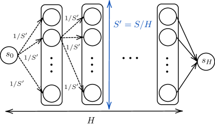
Figure 1: A simple tabular MDP instance for proving a lower bound. The transitions occur uniformly at random to states in the next layer.

4.1 Lower bound for episodic MDPs with adversarial losses

We first provide a construction of a $\Omega(\sqrt{HSAT})$ lower bound for episodic tabular MDPs with adversarial losses, using the above MDP instance.

Theorem 1.

Suppose that $H\geq 3$ and $A\geq 5$. Then, for any policy, there exists an episodic MDP with adversarial losses such that $\mathbb{E}[\mathsf{Reg}_{T}]=\Omega(\sqrt{HSAT})$.

The proof can be found in Appendix˜B. This lower bound matches the regret upper bound of $O(\sqrt{HSAT})$ obtained by the standard approach of running FTRL with the Shannon entropy regularizer over $\Omega$ (Zimin and Neu, 2013).

It is intuitive that the above construction yields a lower bound of $\Omega(\sqrt{HSAT})$. In the above instance, each state is visited $T^{\prime}\coloneqq T/S^{\prime}$ times over $T$ episodes in expectation. Hence, we can view this instance as solving $S$ independent multi-armed bandits, each with $A$ arms and $T^{\prime}$ rounds, whose minimax lower bound is $\Omega(\sqrt{AT^{\prime}})$ (Vogel, 1960; Auer et al., 1995). Therefore, we obtain $\mathbb{E}[\mathsf{Reg}_{T}]\gtrsim S\sqrt{AT^{\prime}}=S\sqrt{A(T/S^{\prime})}\simeq\sqrt{HSAT}$. Specifically, in the proof of Theorem˜1, we construct $\lvert\Pi_{\mathsf{det}}\rvert=A^{S}$ different MDP instances. Each instance $\mathcal{M}_{\mathsf{loss}}(\pi^{\circ})$ has the same transition kernel as shown in Figure˜1, and stochastic loss functions are given by $\ell_{t}(s,a)\sim\mathsf{Ber}(\frac{1}{2}-\varepsilon\mathbbm{1}{\left[a=\pi^{\circ}(s)\right]})$ for each $(s,a)\in\mathcal{S}\times\mathcal{A}$. Then, we can prove the lower bound by an argument similar to the proof of the minimax lower bound for multi-armed bandits (e.g., Auer et al. 1995, Lattimore and Szepesvári 2020, Chapter 15), preparing additional instances $\{\mathcal{M}_{\mathsf{loss}}(\pi^{\circ},\widetilde{s})\}_{\widetilde{s}\in\mathcal{S}}$ with stochastic loss functions $\ell_{t}(s,a)\sim\mathsf{Ber}(\frac{1}{2}-\varepsilon\mathbbm{1}{\left[a=\pi^{\circ}(s),s\neq\widetilde{s}\right]})$ for each $\widetilde{s}\in\mathcal{S}$.

A notable advantage of this lower bound construction is its simplicity: unlike existing constructions (e.g., Jaksch et al. 2010; Jin et al. 2018; Domingues et al. 2021), which involve complex structures such as building $A$-ary trees (though they have the advantage of achieving a tighter lower bound under unknown transitions), our instance is remarkably simple. Thanks to this simplicity, as we will see below, a similar instance can also be used to establish a lower bound for PbMDPs with Borda scores.

4.2 Lower bound for preference-based MDPs with Borda scores

Inspired by the above instance construction and the lower bound construction for dueling bandits with a Borda winner (Saha et al., 2021), we prove the following lower bound for PbMDPs with Borda scores, the proof of which can be found in Appendix˜B.

Theorem 2.

Suppose that $H\geq 3$ and $K\geq 5$. Then, for any policy, there exists an episodic PbMDP with Borda scores such that $\mathbb{E}[\mathsf{Reg}_{T}]=\Omega((H^{2}SK)^{1/3}T^{2/3})$.

The intuition behind this lower bound can also be obtained, similarly to Section˜4.1. We consider an instance based on Figure˜1, and, in this instance, each state is visited $T^{\prime}\coloneqq T/S^{\prime}$ times in expectation over $T$ episodes. Thus, we can view this instance as solving $S$ independent dueling bandits with a Borda winner, each with $K$ arms and $T^{\prime}$ rounds, whose minimax lower bound is $\Omega(K^{1/3}{T^{\prime}}^{2/3})$ (Saha et al., 2021). Hence, we obtain $\mathbb{E}[\mathsf{Reg}_{T}]\gtrsim SK^{1/3}{T^{\prime}}^{2/3}=SK^{1/3}(T/S^{\prime})^{2/3}\simeq(H^{2}SK)^{1/3}T^{2/3}$.

5 Global optimization

This section provides a global optimization algorithm for preference-based MDPs with Borda scores.

5.1 Algorithm design

Here, we describe the design of our algorithm. The full pseudocode is provided in Algorithm˜1.

Reduction to online linear optimization over $\Omega$

From the definitions of the regret and the occupancy measure, the regret can be written as $\mathbb{E}[\mathsf{Reg}_{T}]=\mathbb{E}[\sum_{t=1}^{T}\langle q^{\pi_{t}}-q^{\pi^{*}},\ell_{t}\rangle]$ for $\ell_{t}$ in ˜2. Based on this observation, we can minimize the regret by solving an online linear optimization (OLO) problem over the set of all occupancy measures $\Omega$, a standard approach in the literature on online reinforcement learning (e.g., Even-Dar et al. 2009; Zimin and Neu 2013; Jin et al. 2020a, to name a few). Therefore, if the Borda score can be estimated from observations, it may be possible to minimize the regret.

Borda score estimation

We must estimate the Borda score using only the observed trajectories, i.e., bandit feedback. For this purpose, we consider the following Borda score estimator inspired by the one proposed in Saha et al. (2021) for dueling bandits with a Borda winner. For a policy $\pi_{t}$ used in episode $t$, we define the estimator $\widehat{b}_{t}\colon\mathcal{S}\times[K]\to\mathbb{R}$ by

$$\widehat{b}_{t}(s,i)=\frac{\mathbbm{1}{\left[a_{t,s}^{L}=i\right]}}{K\sum_{j^{\prime}\in[K]}\pi_{t}((i,j^{\prime})\mid s)}\frac{o_{t}(s,a_{t,s}^{L},a_{t,s}^{R})-1}{\sum_{i^{\prime}\in[K]}\pi_{t}((i^{\prime},a_{t,s}^{R})\mid s)}\,,$$ (3)

where $a_{t,s}^{L}$ and $a_{t,s}^{R}$ are the first and second arms chosen at state $s$ in episode $t$, respectively. It is important to note that when $a_{t,s}^{L}$ and $a_{t,s}^{R}$ are independent at state $s$, the estimator $\widehat{b}_{t}(s,i)$ is an unbiased estimator of the Borda score $b_{t}(s,i)$ (see Appendix˜C for the proof).

Epsilon-greedy-type algorithm

As in many problems with minimax regret of $\Theta(T^{2/3})$ (Bartók et al., 2011; Alon et al., 2015; Saha et al., 2021), we incorporate appropriate exploration instead of directly using the output of the OLO algorithm for exploitation. An important point to note here is that, as discussed above, estimating the Borda score relies on the assumption that the arm pair $(a_{t,s}^{L},a_{t,s}^{R})$ is selected independently. If two arms are chosen according to an arbitrary policy, it may not be possible to obtain an unbiased estimate of the Borda score. To address this, we introduce an epsilon-greedy-type procedure: for each episode, we sample from a Bernoulli distribution with parameter $\gamma\in(0,1/2]$ (Line 1) to determine whether to exploit or explore.

In exploitation episodes (Line 1), we solve the OLO problem based on the Borda score estimated from past observations. As the OLO algorithm, we use follow-the-regularized-leader (FTRL) with the negative Shannon entropy regularizer, as defined in ˜4. The purpose of exploitation episodes is to leverage past observations, and no estimation is performed: the Borda score estimator in the exploitation episode is set to $\widetilde{b}_{t}(s,i)=0$ for all $(s,i)\in\mathcal{S}\times[K]$.

In exploration episodes (Line 1), several techniques are incorporated. A key issue is that the Borda score estimator $\widetilde{b}_{t}(s,i)$ (in Line 1) can become arbitrarily large due to the presence of $q^{\pi_{t}}(s)$ in the denominator. The value of $q^{\pi_{t}}(s)$, the probability of reaching state $s$ under the policy $\pi_{t}$ and transition kernel $P$, can be extremely small depending on the properties of $P$. To address this, we focus on a uniformly sampled state $\widetilde{s}_{t}\sim\mathsf{Unif}(\mathcal{S})$ and use the policy $\pi^{r_{\widetilde{s}_{t}}}$ for $r_{\widetilde{s}_{t}}\in\operatorname*{arg\,max}_{q\in\Omega}q(\widetilde{s}_{t})$ until we reach the state $\widetilde{s}_{t}$ (Line 1). This allows us to avoid having terms such as $\min_{s\in\mathcal{S}}q^{\pi}(s)$ for some $\pi$—which are known to appear in regret upper bounds in standard reinforcement learning settings (e.g., Agarwal et al. 2020)—in the denominator of the regret bound.

Once state $\widetilde{s}_{t}$ is reached, the learner switches the policy from $\pi^{r_{\widetilde{s}_{t}}}$ to the uniform policy (Line 1) in order to perform unbiased estimation of the Borda score. We employ an inverse-weighted approach to estimate the Borda score $\widetilde{b}_{t}(s,i)$ (Line 1), setting the estimator to a non-zero value only when the episode is for exploration ($\xi_{t}=1$), the sampled state satisfies $\widetilde{s}_{t}=s$, and state $s$ is visited ($\mathbb{I}_{t}(s)=1$). Specifically, we define $\widetilde{b}_{t}(s,i)$ based on $\widehat{b}_{t}(s,i)$ in ˜3 as $\widetilde{b}_{t}(s,i)=\frac{S}{q^{\pi_{t}}(s)\gamma}\mathbbm{1}{\left[\xi_{t}=1,\widetilde{s}_{t}=s\right]}\mathbb{I}_{t}(s)\widehat{b}_{t}(s,i).$ One can see that, with Algorithm˜1, this estimator $\widetilde{b}_{t}(s,i)$ is an unbiased estimator for $b_{t}(s,i)$ and thus the estimator $\widehat{\ell}_{t}(s,a)=-\frac{1}{2}(\widetilde{b}_{t}(s,a^{L})+\widetilde{b}_{t}(s,a^{R}))$ is also an unbiased estimator for $\ell_{t}(s,a)$.

1 Input: exploration rate $\gamma\in(0,1/2]$, learning rate $\eta>0$

2 Compute $r_{s}=\operatorname*{arg\,max}_{q\in\Omega}q(s)$ for each state $s\in\mathcal{S}$.

3 for each episode $t=1,2,\dots,T$ do

4    Sample $\xi_{t}\sim\mathsf{Ber}(\gamma)$.

5    if $\xi_{t}=0$ then

6       Compute $\widetilde{q}_{t}\in\Omega$ by FTRL with the negative Shannon entropy regularizer:

$$\widetilde{q}_{t}\in\operatorname*{arg\,min}_{q\in\Omega}\left\{\left\langle q,\sum_{\tau=1}^{t-1}\widehat{\ell}_{\tau}\right\rangle\!-\frac{1}{\eta}\operatorname{H}(q)\right\}\,,\ \operatorname{H}(q)=\!\!\!\!\!\!\sum_{(s,a)\in\mathcal{S}\times\mathcal{A}}q(s,a)\log\left(\frac{1}{q(s,a)}\right)\,.$$ (4)

7       Execute policy $\widetilde{\pi}_{t}\coloneqq\pi^{\widetilde{q}_{t}}$ given by $\widetilde{\pi}_{t}(a\mid s)={\widetilde{q}_{t}(s,a)}/{\widetilde{q}_{t}(s)}$.

8   else

9       Sample $\widetilde{s}_{t}\sim\mathsf{Unif}(\mathcal{S})$ and execute policy $\pi^{r_{\widetilde{s}_{t}}}$ and stop if the learner reaches state $\widetilde{s}_{t}$.

10       Sample two arms $a_{t,\widetilde{s}_{t}}^{L},a_{t,\widetilde{s}_{t}}^{R}\sim\mathsf{Unif}([K])$ uniformly at random.

11       Execute arbitrary policy for the remaining steps.

12   Compute $\widetilde{b}_{t}(s,i)\!=\!\frac{S}{\gamma q^{\pi_{t}}(s)}\mathbbm{1}{\left[\xi_{t}=1,\widetilde{s}_{t}=s\right]}\,\mathbb{I}_{t}(s)\,\widehat{b}_{t}(s,i)$ for $s\in\mathcal{S},i\in[K]$ for $\widehat{b}_{t}$ in ˜3 .

13    Compute the estimator by $\widehat{\ell}_{t}(s,a)=-\frac{1}{2}\big{(}\widetilde{b}_{t}(s,a^{L})+\widetilde{b}_{t}(s,a^{R})\big{)}$ for each $(s,a)\in\mathcal{S}\times\mathcal{A}$.

Algorithm 1 Global optimization for preference-based MDPs with Borda scores

Remark 1.

In the algorithm for adversarial dueling bandits with a Borda winner (Saha et al., 2021), instead of considering policies over $\mathcal{A}=[K]\times[K]$ as we do, the algorithm samples $a_{t}^{L}$ and $a_{t}^{R}$ independently from a probability distribution over $[K]$ determined by FTRL. This allows them to construct an unbiased estimator of the Borda score. However, such an approach—selecting arms independently—is not applicable in our setting of PbMDPs with Borda scores since the transitions are determined by the joint arm pair $(a_{t,s}^{L},a_{t,s}^{R})$.

5.2 Regret upper bound

The above algorithm achieves the following bound, the proof of which can be found in Appendix˜C.

Theorem 3.

Suppose that $T\geq 8S^{2}K\log(SK)/H^{2}$. Then, with appropriate choices of $\eta$ and $\gamma$, Algorithm˜1 achieves $\mathbb{E}[\mathsf{Reg}_{T}]=O\left((H^{2}S^{2}K)^{1/3}T^{2/3}(\log(SK))^{1/3}\right)$

The regret upper bound in Theorem˜3 has a $\widetilde{O}(S^{1/3})$ gap compared to the lower bound in Theorem˜2. This suboptimality arises from the uniform sampling of states in exploration episodes. Since $S$ can be very large in many reinforcement learning tasks, this dependence may be undesirable, which we address in the next section. When $H=S=1$, PbMDPs with Borda scores is reduced to the dueling bandits with a Borda winner and our bound becomes $\mathbb{E}[\mathsf{Reg}_{T}]=O\left((K\log K)^{1/3}T^{2/3}\right)$, which matches the minimax regret in Saha et al. (2021, Theorems 2 and 6) up to a logarithmic factor.

6 Policy optimization

In the global optimization approach of the previous section, the regret upper bound has a suboptimal dependence of $S^{2/3}$. Moreover, the global optimization approach is computationally inefficient, as it requires solving a convex optimization problem over $\Omega$ in every episode, and is also difficult to extend to structured MDPs. To address these issues, this section presents a policy optimization algorithm.

6.1 Algorithm design

Here, we describe the design of our algorithm. The full pseudocode is provided in Algorithm˜2.

Reduction to online linear optimization over simplex

One of the most representative approaches to implementing policy optimization in episodic MDPs is to leverage the following performance difference lemma (Kakade and Langford, 2002): for any policies $\pi,\pi^{*}\in\Pi$ and function $\ell\colon\mathcal{S}\times\mathcal{A}\to[0,1]$, it holds that $V^{\pi}(s_{0};\ell)-V^{\pi^{*}}(s_{0};\ell)=\sum_{s\in\mathcal{S}}q^{\pi^{*}}(s)\left\langle\pi(\cdot\mid s)-\pi^{*}(\cdot\mid s),Q^{\pi}(s,\cdot;\ell)\right\rangle.$ Using this equality, we can rewrite the regret as

$$\mathsf{Reg}_{T}=\sum_{s\in\mathcal{S}}q^{\pi^{*}}(s)\sum_{t=1}^{T}\left\langle\pi_{t}(\cdot\mid s)-\pi^{*}(\cdot\mid s),Q^{\pi_{t}}(s,\cdot;\ell_{t})\right\rangle\,.$$ (5)

Hence, it suffices to solve an online linear optimization problem over $\Delta(\mathcal{A})$ with gradient vector $Q^{\pi_{t}}(s,\cdot;\ell_{t})\in[0,H]^{A}$ for each state $s\in\mathcal{S}$ to minimize the regret. As in the case of the previous section, we need to estimate the Q-function $Q^{\pi_{t}}(s,a;\ell_{t})$ used for the gradient from observed trajectories. Below, we will provide a Q-function estimator and present an FTRL-based algorithm inspired by Luo et al. (2021).

1 Input: learning rate $\eta>0$, exploration rate $\gamma\in(0,1/2]$, bias parameter $\delta>0$, constant $c>0$

2

3for each episode $t=1,2,\dots,T$ do

4    for each state $s\in\mathcal{S}$ do

5       Sample $\xi_{t}(s)\sim\mathsf{Ber}(\gamma)$.

6       if $\xi_{t}(s)=0$ then  Set $\widetilde{\pi}_{t}(\cdot\mid s)\propto\exp\big{(}-\eta\sum_{\tau=1}^{t-1}(\widehat{Q}_{\tau}-M_{\tau})\big{)}$ for $s\in\mathcal{S}$ and $\pi_{t}\leftarrow\widetilde{\pi}_{t}$.

7       else  Set $\pi_{t}(\cdot\mid s)\leftarrow\pi_{0}(\cdot\mid s)\coloneqq 1/A$.

8      

9   Execute policy $\pi_{t}$, obtain a trajectory $\{(s_{t,h},a_{t,h},o_{t}(s_{t,h},a_{t,h}))\}_{h=0}^{H-1}$, and compute

$$\widehat{\ell}_{t}(s,a)\!=\!-\frac{\mathbbm{1}{\left[\xi_{t}(s)\!=\!1\right]}}{\gamma}\widehat{B}_{t}(s,a)\,,\ \widehat{B}_{t}(s,a)\!=\!\frac{1}{2}(\widehat{b}_{t}(s,a^{L})\!+\!\widehat{b}_{t}(s,a^{R}))\,,\ \widehat{b}_{t}(s,i)\!=\!\mbox{\lx@cref{creftypecap~refnum}{eq:def_b_hat}}\,,\vskip-2.0pt$$ (6)

10    For $\pi^{\circ}_{t}(\cdot\mid s)=(1-\gamma)\widetilde{\pi}_{t}(\cdot\mid s)+\gamma\frac{1}{A}$ and $q_{t}=q^{\pi_{t}^{\circ}}\in\Omega$, estimate the Q-function by

$$\widehat{Q}_{t}(s,a)\!=\!\frac{q_{t}(s,a)}{q_{t}(s,a)\!+\!\delta}\frac{\mathbb{I}_{t}(s,a)}{q_{t}(s)/A}\widehat{\ell}_{t}(s,a)+\frac{\mathbb{I}_{t}(s,a)}{q_{t}(s,a)\!+\!\delta}\widehat{L}_{t,h(s)+1}\,,\ \widehat{L}_{t,h}\!=\!\sum_{k=h}^{H-1}\!w_{t,k}\widehat{\ell}_{t}(s_{t,k},a_{t,k})\,,\vskip-8.0pt$$ (7)

where $w_{t,k}={\pi^{\circ}_{t}(a_{t,k}\mid s_{t,k})}/{\pi_{0}(a_{t,k}\mid s_{t,k})}$.

11    Compute the bonus term by

$$M_{t}(s,a)=Q^{\pi_{t}}(s,a;m_{t})\,,\quad m_{t}(s)=m_{t}(s,a)=\sum_{a^{\prime}\in\mathcal{A}}\frac{c\,\delta H\widetilde{\pi}_{t}(a^{\prime}\mid s)}{q_{t}(s,a^{\prime})+\delta}\,.$$ (8)

Algorithm 2 Policy optimization for preference-based MDPs with Borda scores

Epsilon-greedy-type algorithm

As in the case of global optimization, we consider an epsilon-greedy-type algorithm: for each state $s$, we sample $\xi_{t}(s)$ from a Bernoulli distribution with parameter $\gamma$ (Line 2), and based on its value, we determine whether to perform exploration or exploitation at that state. In exploitation episodes (Line 2), we use FTRL with the negative Shannon entropy regularizer over $\Delta(\mathcal{A})$ w.r.t. the gradient defined by the difference between an estimated Q-function $\widehat{Q}_{t}$ and a bonus term $M_{t}$ (both defined below) as the OLO algorithm. By contrast to the global optimization case, this update admits a closed-form expression. The estimator $\widehat{Q}_{t}$ is carefully designed, as explained below. In exploration episodes (Line 2), in contrast to the global optimization approach, exploration in the policy optimization approach is remarkably simple: we use the uniform policy $\pi_{0}$ for all states.

Q-function estimation

We now describe how to estimate Q-functions. The construction of the Borda score estimator $\widehat{b}_{t}(s,i)$ is the same as in Section˜5. In contrast to the previous section, we do not use $\widetilde{b}_{t}(s,i)$ here; instead, we directly estimate Q-functions based on $\widehat{b}_{t}(s,i)$ in (3). To do so, we first compute the unbiased inverse-weighted loss estimators $\widehat{\ell}_{t}$ in ˜6 using $\widehat{b}_{t}$. We then define the Q-function estimator $\widehat{Q}_{t}(s,a)$ as in ˜7. This $\widehat{Q}_{t}(s,a)$ is an unbiased estimator of $Q^{\pi_{t}}(s,a)$ when $\delta=0$ (see Appendix˜D for the proof). The estimator $\widehat{Q}_{t}(s,a)$ is carefully designed: since the Borda score estimator is non-zero only in the exploration episodes, the definition of the cumulative loss estimator $\widehat{L}_{t,h}$ for steps after $h$ incorporates importance weighting to correct for this bias. Note that in our algorithm, importance weighting is not needed for the transitions.

Bonus term

Our algorithm computes a bonus term defined in ˜8, which is used in FTRL. Intuitively, this term encourages exploration of states that are visited less frequently. In the regret analysis, it serves to correct for the discrepancy between the occupancy measure $q^{\pi^{*}}$ of the optimal policy and the occupancy measure $q_{t}$. For further background, we refer the reader to Luo et al. (2021).

6.2 Regret upper bound

The above algorithm achieves the following bound, the proof of which can be found in Appendix˜D.

Theorem 4.

Suppose that $T\geq(SK^{5}\log K)/(\alpha H^{3})$. Then, with appropriate choices of $c>0$, $\eta\leq 1/(cH)$, $\gamma\in(0,1/2]$, and $\delta>0$, Algorithm˜2 achieves $\mathbb{E}[\mathsf{Reg}_{T}]=\widetilde{O}\big{(}(H^{6}SK^{5})^{1/3}T^{2/3}+H^{4}T^{1/3}/(SK^{5})^{1/3}\big{)}.$

The regret upper bound in Theorem˜4 improves the dependence on $S$ from $S^{2/3}$ to $S^{1/3}$ compared to Theorem˜3, while with the same dependence on $T$ and worse dependence on $H$ and $K$. In addition, it benefits from the advantages of policy optimization: efficient computation and natural extensibility to structured MDPs.

6.3 Extension to unknown-transition case

The results so far are for the known-transition setting. Our analysis can be extended to the unknown-transition setting by adopting an approach similar to existing algorithms for unknown transitions (Jin et al., 2020a). Briefly, we construct confidence intervals for the transition kernel based on transitions observed in past episodes, and then build loss estimators using the corresponding upper and lower occupancy measures. The details are deferred to Appendix˜E.

7 Conclusion, limitation, and future work

This study proposed a new framework of episodic MDPs with adversarial preferences, called preference-based MDPs (PbMDPs). In particular, we analyzed regret upper and lower bounds in PbMDPs where the loss functions are defined based on the Borda scores. We established the lower bound by constructing a new instance that differs from those used in existing studies on MDPs with adversarial losses. We also presented two algorithms based on both global optimization and policy optimization approaches.

There are many interesting directions for future work. One limitation of this work is the gap between the regret upper and lower bounds. We believe that the lower bound cannot be improved, and therefore, it is an important direction to investigate whether the upper bound can be improved through new algorithmic designs or refined analyses. A second limitation is that our study focuses solely on the Borda score as the loss functions of PbMDPs. It would be valuable to consider alternative preference-based scores—e.g., the Condorcet winner (Urvoy et al., 2013; Zoghi et al., 2014; Komiyama et al., 2015)—and investigate algorithms and regret analysis for such formulations. Another important direction, motivated by prior work on dueling bandits (Saha et al., 2021) and MDPs (Simchowitz and Jamieson, 2019), is to investigate the stochastic setting of PbMDPs, in which the preference function is fixed throughout all episodes. In particular, it would be desirable to achieve best-of-both-worlds performance, optimal in both stochastic and adversarial settings. It is an open question whether techniques developed for best-of-both-worlds reinforcement learning in MDPs (Jin and Luo, 2020; Dann et al., 2023) can be combined with learning rates for problems with minimax regret of $T^{2/3}$ (Tsuchiya and Ito, 2024). Extending the policy optimization approach to settings where the loss functions or transition kernel have structural properties (see e.g., Jin et al. 2020b; Cai et al. 2020; Neu and Olkhovskaya 2021) is also an important direction for future work.

Appendix A Additional related work

In this section, we discuss additional related work that could not be included in the main body.

The problem of learning in preference-based MDPs can be viewed as an extension of adversarial dueling bandit problems to settings with state transitions. As discussed in the main body, dueling bandit problems have been studied under various assumptions. For a more comprehensive background, we refer the reader to the survey on dueling bandits by Bengs et al. (2021).

In the main body, we noted that extending to notions such as the Condorcet winner would be an interesting direction. Another promising direction, inspired by the existing literature on dueling bandits, is to consider formulations based on the von Neumann winner, originally proposed in the context of contextual dueling bandits by DudÃk et al. (2015). The von Neumann winner is defined as a randomized policy (over the set of arms) that beats or ties with any randomized policy of the opponent arm. Similar to the Borda winner, the von Neumann winner is guaranteed to exist and enjoyes several desirable properties. It would also be interesting to explore the connection between our framework of preference-based MDPs and contextual dueling bandits under stochastic contexts (e.g., Saha 2021).

Our work can also be viewed in the context of preference-based reinforcement learning (PbRL). Most existing studies on PbRL assume a fixed probabilistic structure underlying the preferences that remains unchanged across all episodes. For a detailed background, we refer the reader to the survey on PbRL by Wirth et al. (2017) and the references in more recent works (Christiano et al., 2017; Novoseller et al., 2020; Hejna and Sadigh, 2023; Saha et al., 2023; Wu and Sun, 2024). As discussed in the main body, to the best of our knowledge, our work is the first to establish the problem of learning from adversarial preferences with state transitions.

Appendix B Deferred proofs of lower bounds from Section˜4

This section provides deferred proofs of lower bounds from Section˜4. Here, we use $\mathrm{D}(\mathbb{P},\mathbb{P}^{\prime})$ to denote the Kullback–Leibler (KL) divergence between distributions $\mathbb{P}$ and $\mathbb{P}^{\prime}$, and use $\mathrm{kl}(p,q)$ to denote the KL divergence between Bernoulli distributions with means $p$ and $q$. Let $\widetilde{\mathcal{S}}=\mathcal{S}\setminus\{s_{0}\}$ (recall that we may use $\mathcal{S}$ to denote $\mathcal{S}\setminus\{s_{H}\}$ for simplicity) and we use

$$N_{T}(s,a)=\sum_{t=1}^{T}\frac{1}{S^{\prime}}\,\pi_{t}(a\mid s)$$

to denote the expected number of times the state-action pair $(s,a)\in\widetilde{\mathcal{S}}\times\mathcal{A}$ is visited.

B.1 Proof of Theorem˜1

Here we provide the proof of Theorem˜1.

Proof of Theorem˜1.

Let $\varepsilon\in(0,1/4]$. We consider the following instances. For each $\pi^{\circ}\in\Pi_{\mathsf{det}}$, we define an episodic MDP with stochastic losses $\mathcal{M}_{\mathsf{loss}}(\pi^{\circ})$ as follows:

• The transitions occur uniformly at random to states in the next layer; that is, for any $(s,a)\in\mathcal{S}_{h}\times\mathcal{A}$, it holds that $P(s^{\prime}\mid s,a)=1/S_{h+1}$ for all $s^{\prime}\in\mathcal{S}_{h+1}$.

• Each loss function follows a Bernoulli distribution given by

  $$\ell_{t}(s,a)\sim\begin{cases}\mathsf{Ber}(1/2-\varepsilon)&\mbox{if}\ a=\pi^{\circ}(s)\,,\\ \mathsf{Ber}(1/2)&\mbox{otherwise}\,.\end{cases}$$

We use $\mathbb{E}^{(\pi^{\circ})}[\cdot]$ to denote the expectation under the episodic MDP $\mathcal{M}_{\mathsf{loss}}(\pi^{\circ})$ and we recall $\widetilde{\mathcal{S}}=\mathcal{S}\setminus\{s_{0}\}$. Then, we can rewrite the regret under $\mathcal{M}_{\mathsf{loss}}(\pi^{\circ})$ as

$$\mathbb{E}^{(\pi^{\circ})}[\mathsf{Reg}_{T}] \geq\varepsilon(H-1)T-\varepsilon\sum_{s\in\widetilde{\mathcal{S}}}\mathbb{E}^{(\pi^{\circ})}\left[N_{T}(s,\pi^{\circ}(s))\right]$$

$$=\frac{\varepsilon T}{S^{\prime}}\Bigg{(}S^{\prime}(H-1)-\frac{S^{\prime}}{T}\sum_{s\in\widetilde{\mathcal{S}}}\mathbb{E}^{(\pi^{\circ})}\left[N_{T}(s,\pi^{\circ}(s))\right]\Bigg{)}\,.$$ (9)

In what follows, we will upper bound $\mathbb{E}^{(\pi^{\circ})}\left[N_{T}(s,\pi^{\circ}(s))\right]$. To do so, for each $(\pi^{\circ},\widetilde{s})\in\Pi_{\mathsf{det}}\times\mathcal{S}$, we consider the following $\mathcal{M}_{\mathsf{loss}}(\pi^{\circ},\widetilde{s})$, an instance of episodic MDPs with stochastic losses:

• The transitions occur uniformly at random to states in the next layer; that is, for any $(s,a)\in\mathcal{S}_{h}\times\mathcal{A}$, it holds that $P(s^{\prime}\mid s,a)=1/S_{h+1}$ for all $s^{\prime}\in\mathcal{S}_{h+1}$.

• Each loss function follows a Bernoulli distribution given by

  $$\ell_{t}(s,a)\sim\begin{cases}\mathsf{Ber}(1/2-\varepsilon)&\mbox{if}\ a=\pi^{\circ}(s)\ \mbox{and}\ s\neq\widetilde{s}\,,\\ \mathsf{Ber}(1/2)&\mbox{otherwise}\,.\end{cases}$$

Note that the only difference between $\mathcal{M}_{\mathsf{loss}}(\pi^{\circ})$ and $\mathcal{M}_{\mathsf{loss}}(\pi^{\circ},\widetilde{s})$ lies in the expected value of the loss at the state-action pair $(\widetilde{s},\pi^{\circ}(\widetilde{s}))$. We use $\mathbb{E}^{(\pi^{\circ},\widetilde{s})}[\cdot]$ to denote the expectation under $\mathcal{M}_{\mathsf{loss}}(\pi^{\circ},\widetilde{s})$.

Let $\mathbb{P}_{\pi^{\circ}}$ and $\mathbb{P}_{\pi^{\circ},\widetilde{s}}$ be the probability distribution induced by $\mathcal{M}_{\mathsf{loss}}(\pi^{\circ})$ and $\mathcal{M}_{\mathsf{loss}}(\pi^{\circ},\widetilde{s})$, respectively. Then, using the fact that $\frac{S^{\prime}}{T}N_{T}(s,\pi^{\circ}(s))\in[0,1]$ for $s\neq s_{0}$ and Pinsker’s inequality, for any $\widetilde{s}\in\mathcal{S}\setminus\{s_{0}\}$ we have

$$\frac{S^{\prime}}{T}\mathbb{E}^{(\pi^{\circ})}\left[N_{T}(\widetilde{s},\pi^{\circ}(\widetilde{s}))\right] \leq\frac{S^{\prime}}{T}\mathbb{E}^{(\pi^{\circ},\widetilde{s})}\left[N_{T}(\widetilde{s},\pi^{\circ}(\widetilde{s}))\right]+\mathrm{TV}(\mathbb{P}_{\pi^{\circ}},\mathbb{P}_{\pi^{\circ},\widetilde{s}})$$

$$\leq\frac{S^{\prime}}{T}\mathbb{E}^{(\pi^{\circ},\widetilde{s})}\left[N_{T}(\widetilde{s},\pi^{\circ}(\widetilde{s}))\right]+\sqrt{\frac{1}{2}\mathrm{D}(\mathbb{P}_{\pi^{\circ},\widetilde{s}},\mathbb{P}_{\pi^{\circ}})}\,.$$ (10)

Then, from the chain rule of the KL divergence, we can evaluate the KL divergence in the last inequality as

$$\mathrm{D}(\mathbb{P}_{\pi^{\circ},\widetilde{s}},\mathbb{P}_{\pi^{\circ}})=\mathbb{E}^{(\pi^{\circ},\widetilde{s})}\left[N_{T}(\widetilde{s},\pi^{\circ}(\widetilde{s}))\right]\,\mathrm{kl}(1/2,1/2-\varepsilon)\leq 4\varepsilon^{2}\mathbb{E}^{(\pi^{\circ},\widetilde{s})}\left[N_{T}(\widetilde{s},\pi^{\circ}(\widetilde{s}))\right]\,,$$ (11)

where we used $\mathrm{kl}(1/2,1/2-\varepsilon)\leq 4\varepsilon^{2}$ for $\varepsilon\in(0,1/4]$. Taking the uniform average over $\Pi_{\mathsf{det}}$ for the RHS of ˜11, for any $\widetilde{s}\in\widetilde{\mathcal{S}}$ we have

$$\mathbb{E}_{\pi^{\circ}\sim\mathsf{Unif}(\Pi_{\mathsf{det}})}\left[\mathbb{E}^{(\pi^{\circ},\widetilde{s})}\left[N_{T}(\widetilde{s},\pi^{\circ}(\widetilde{s}))\right]\right]$$

$$=\sum_{a\in\mathcal{A}}\Pr[\pi^{\circ}(\widetilde{s})=a]\ \mathbb{E}_{\pi^{\circ}\sim\mathsf{Unif}(\Pi_{\mathsf{det}})}\left[\mathbb{E}^{(\pi^{\circ},\widetilde{s})}\left[N_{T}(\widetilde{s},\pi^{\circ}(\widetilde{s}))\right]\mathrel{}\middle|\mathrel{}\pi^{\circ}(\widetilde{s})=a\right]$$

$$=\frac{1}{A}\sum_{a\in\mathcal{A}}\mathbb{E}_{\pi^{\circ}\sim\mathsf{Unif}(\Pi_{\mathsf{det}})}\left[\mathbb{E}^{(\pi^{\circ},\widetilde{s})}\left[N_{T}(\widetilde{s},a)\right]\right]=\frac{T}{S^{\prime}A}\,,$$ (12)

where the last equality follows from the definition of $N_{T}$. By summing over $\widetilde{s}\in\widetilde{\mathcal{S}}$ in ˜12,

$$\sum_{\widetilde{s}\in\widetilde{\mathcal{S}}}\mathbb{E}_{\pi^{\circ}\sim\mathsf{Unif}(\Pi_{\mathsf{det}})}\left[\mathbb{E}^{(\pi^{\circ},\widetilde{s})}\left[N_{T}(\widetilde{s},\pi^{\circ}(\widetilde{s}))\right]\right]=\frac{(S-2)T}{S^{\prime}A}=\frac{(H-1)T}{A}\,,$$ (13)

where we used $S^{\prime}=(S-2)/(H-1)$ in the last equality. Using the last inequality, we also have

$$\mathbb{E}_{\pi^{\circ}\sim\mathsf{Unif}(\Pi_{\mathsf{det}})}\left[\sum_{\widetilde{s}\in\widetilde{\mathcal{S}}}\sqrt{\frac{1}{2}\mathrm{D}(\mathbb{P}_{\pi^{\circ},\widetilde{s}},\mathbb{P}_{\pi^{\circ}})}\right]\leq\varepsilon\,\mathbb{E}_{\pi^{\circ}\sim\mathsf{Unif}(\Pi_{\mathsf{det}})}\left[\sum_{\widetilde{s}\in\widetilde{\mathcal{S}}}\sqrt{2\mathbb{E}^{(\pi^{\circ},\widetilde{s})}\left[N_{T}(\widetilde{s},\pi^{\circ}(\widetilde{s}))\right]}\right]$$

$$\qquad\leq\sqrt{2(S-2)\sum_{\widetilde{s}\in\widetilde{\mathcal{S}}}\mathbb{E}_{\pi^{\circ}\sim\mathsf{Unif}(\Pi_{\mathsf{det}})}\mathbb{E}^{(\pi^{\circ},\widetilde{s})}\left[N_{T}(\widetilde{s},\pi^{\circ}(\widetilde{s}))\right]}\leq\sqrt{\frac{2HST}{A}}\,,$$ (14)

where the first inequality follows from ˜11, the second inequality follows from the Cauchy–Schwarz inequality and Jensen’s inequality, and the last inequality follows from ˜13.

Finally, combining everything together and recalling that $S^{\prime}=(S-2)/(H-1)$, we have

$$\max_{\pi^{\circ}\in\Pi_{\mathsf{det}}}\mathbb{E}^{(\pi^{\circ})}\left[\mathsf{Reg}_{T}\right] \geq\mathbb{E}_{\pi^{\circ}\sim\mathsf{Unif}(\Pi_{\mathsf{det}})}\left[\mathbb{E}^{(\pi^{\circ})}\left[\mathsf{Reg}_{T}\right]\right]$$

$$\geq\frac{\varepsilon T}{S^{\prime}}\Bigg{(}\frac{S}{2}-\frac{S^{\prime}}{T}\sum_{s\in\widetilde{\mathcal{S}}}\mathbb{E}_{\pi^{\circ}\sim\mathsf{Unif}(\Pi_{\mathsf{det}})}\left[\mathbb{E}^{(\pi^{\circ})}\left[N_{T}(s,\pi^{\circ}(s))\right]\right]\Bigg{)}$$

$$\geq\frac{\varepsilon T}{S^{\prime}}\Bigg{(}\frac{S}{2}-\frac{S^{\prime}}{T}\mathbb{E}_{\pi^{\circ}\sim\mathsf{Unif}(\Pi_{\mathsf{det}})}\Bigg{[}\sum_{s\in\widetilde{\mathcal{S}}}\mathbb{E}^{(\pi^{\circ},s)}\left[N_{T}(s,\pi^{\circ}(s))\right]\Bigg{]}$$

$$\qquad\qquad\qquad\quad-\varepsilon\,\mathbb{E}_{\pi^{\circ}\sim\mathsf{Unif}(\Pi_{\mathsf{det}})}\Bigg{[}\sum_{s\in\widetilde{\mathcal{S}}}\sqrt{\frac{1}{2}\mathrm{D}(\mathbb{P}_{\pi^{\circ},s},\mathbb{P}_{\pi^{\circ}})}\Bigg{]}\Bigg{)}$$

$$\geq\frac{\varepsilon T}{S^{\prime}}\left(\frac{S}{2}-\frac{2HS^{\prime}}{A}-\varepsilon\sqrt{\frac{2HST}{A}}\right)$$

$$\geq\frac{\varepsilon HT}{2}\left(\frac{1}{2}-\frac{4}{A}-\varepsilon\sqrt{\frac{2HT}{SA}}\right)\,,$$

where the last inequality follows from the assumption that $H\geq 3$. Choosing the optimal $\varepsilon$ in the last inequality and using the assumption that $A\geq 5$ complete the proof. ∎

B.2 Proof of Theorem˜2

Here we provide the proof of Theorem˜2. We use $A[i,j]$ to denote the $(i,j)$-element of matrix $A$. For simplicity, we assume that the number of arms $K$ is even, and let $\widetilde{K}=K/2$. We separate the set of arms into two sets: let $\mathcal{K}_{g}=[\widetilde{K}]=\{1,\dots,K/2\}$ be the set of ‘good’ arms, and $\mathcal{K}_{b}=[K]\setminus\mathcal{K}_{g}$ be the set of ‘bad’ arms. We then define preference matrices $\mathsf{P}\in[0,1]^{K\times K}$ and $\mathsf{P}^{(m)}\in[0,1]^{K\times K}$ for each $m\in[\widetilde{K}]$ by

$$\mathsf{P}=\left(\begin{array}[]{@{\hspace{4pt}}c|c@{\hspace{4pt}}}\hskip 4.0pt\lx@intercol\hfil 0.5\,\mathbf{1}_{\widetilde{K}\times\widetilde{K}}&0.9\,\mathbf{1}_{\widetilde{K}\times\widetilde{K}}\hfil\hskip 4.0\\[8.0pt] \hline\cr\hskip 4.0pt\lx@intercol\hfil\rule{0.0pt}{12.0pt}0.1\,\mathbf{1}_{\widetilde{K}\times\widetilde{K}}&0.5\,\mathbf{1}_{\widetilde{K}\times\widetilde{K}}\hfil\hskip 4.0\end{array}\right)\,,\ \mathsf{P}^{(m)}=\left(\begin{array}[]{@{\hspace{4pt}}c|c@{\hspace{4pt}}}\hskip 4.0pt\lx@intercol\hfil 0.5\,\mathbf{1}_{\widetilde{K}\times\widetilde{K}}&0.9\,\mathbf{1}_{\widetilde{K}\times\widetilde{K}}+2\varepsilon\,e_{m}\mathbf{1}_{\widetilde{K}}^{\!\top}\hfil\hskip 4.0\\[8.0pt] \hline\cr\hskip 4.0pt\lx@intercol\hfil\rule{0.0pt}{12.0pt}0.1\,\mathbf{1}_{\widetilde{K}\times\widetilde{K}}-2\varepsilon\,\mathbf{1}_{\widetilde{K}}e_{m}^{\!\top}&0.5\,\mathbf{1}_{\widetilde{K}\times\widetilde{K}}\hfil\hskip 4.0\end{array}\right)\,,$$

where $\mathbf{1}_{\widetilde{K}\times\widetilde{K}}$ denotes the $\widetilde{K}\times\widetilde{K}$ all-ones matrix. Note that the preference matrix $\mathsf{P}^{(m)}$ is obtained by replacing the $m$-th column of the lower-left block of $\mathsf{P}$ from $0.1$ to $0.1-2\varepsilon$, and replacing the $m$-th row of the upper-right block from $0.9$ to $0.9+2\varepsilon$.

Suppose that the preference function $\mathsf{P}_{t}\colon\mathcal{S}\times[K]\times[K]\to[0,1]$ is given by $\mathsf{P}_{t}(s,i,j)=\mathsf{P}[i,j]$ at some state $s\in\mathcal{S}$. Then, the shifted Borda score defined in ˜2 at state $s$ is

$$b_{t}(s,i)=\begin{cases}-0.3&\mbox{if}\ i\in\mathcal{K}_{g}\,,\\ -0.7&\mbox{if}\ i\in\mathcal{K}_{b}\,.\end{cases}$$

If $\mathsf{P}_{t}(s,i,j)=\mathsf{P}^{(m)}[i,j]$ at some state $s\in\mathcal{S}$, then the shifted Borda score at state $s$ is

$$b_{t}(s,i)=\begin{cases}-0.3&\mbox{if}\ i\in\mathcal{K}_{g}\setminus\{m\}\,,\\ -0.3+\varepsilon&\mbox{if}\ i=m\,,\\ -0.7-2\varepsilon/K&\mbox{if}\ i\in\mathcal{K}_{b}\,.\end{cases}$$

under which the optimal arm is $m\in\mathcal{K}_{g}$. We will use the above definitions to prove Theorem˜2.

Proof of Theorem˜2.

Let $\varepsilon\in(0,1/20]$ and we use

$$\Pi_{\mathsf{pref}}=\{\pi\colon s\mapsto(i,i)\colon s\in\mathcal{S},\,i\in\mathcal{K}_{g}\}$$

to denote the set of all policies in the preference-based MDP that choose the same good arm, and this satisfies $\lvert\Pi_{\mathsf{pref}}\rvert=\widetilde{K}^{S}$. Let $\nu^{\circ}(s)\in\mathcal{K}_{g}$ be an arm satisfying $\pi^{\circ}(s)=(\nu^{\circ}(s),\nu^{\circ}(s))\in\mathcal{A}$. Then, for each $\pi^{\circ}\in\Pi_{\mathsf{pref}}$, define a preference-based MDP $\mathcal{M}_{\mathsf{pref}}(\pi^{\circ})$ as follows:

• The transitions occur uniformly at random to states in the next layer; that is, for any $(s,a)\in\mathcal{S}_{h}\times\mathcal{A}$, it holds that $P(s^{\prime}\mid s,a)=1/S_{h+1}$ for all $s^{\prime}\in\mathcal{S}_{h+1}$.

• The preference function $\mathsf{P}_{t}\colon\mathcal{S}\times[K]\times[K]\to[0,1]$ is given by

  $$\mathsf{P}_{t}(s,i,j)=\mathsf{P}^{(\nu^{\circ}(s))}[i,j]\,,$$

  where the preference matrix is chosen so that the action $\pi^{\circ}(s)$ is optimal at each state $s\in\mathcal{S}$.

We use $\mathbb{E}^{(\pi^{\circ})}[\cdot]$ to denote the expectation under $\mathcal{M}_{\mathsf{pref}}(\pi^{\circ})$. Then, we can rewrite the regret under $\mathcal{M}_{\mathsf{pref}}(\pi^{\circ})$ as

$$\mathbb{E}^{(\pi^{\circ})}[\mathsf{Reg}_{T}] \geq\varepsilon(H-1)T-\varepsilon\sum_{s\in\widetilde{\mathcal{S}}}\mathbb{E}^{(\pi^{\circ})}\left[N_{T}(s,\pi^{\circ}(s))\right]$$

$$=\frac{\varepsilon T}{S^{\prime}}\Bigg{(}S^{\prime}(H-1)-\frac{S^{\prime}}{T}\sum_{s\in\widetilde{\mathcal{S}}}\mathbb{E}^{(\pi^{\circ})}\left[N_{T}(s,\pi^{\circ}(s))\right]\Bigg{)}\,.$$ (15)

In what follows, we will upper bound $\mathbb{E}^{(\pi^{\circ})}\left[N_{T}(s,\pi^{\circ}(s))\right]$. To do so, for each $(\pi^{\circ},\widetilde{s})\in\Pi_{\mathsf{pref}}\times\mathcal{S}$, we consider the following $\mathcal{M}_{\mathsf{pref}}(\pi^{\circ},\widetilde{s})$, an instance of preference-based MDPs:

• The transitions occur uniformly at random to states in the next layer; that is, for any $(s,a)\in\mathcal{S}_{h}\times\mathcal{A}$, it holds that $P(s^{\prime}\mid s,a)=1/S_{h+1}$ for all $s^{\prime}\in\mathcal{S}_{h+1}$.

• The preference function $\mathsf{P}_{t}\colon\mathcal{S}\times[K]\times[K]\to[0,1]$ is given by

  $$\mathsf{P}_{t}(s,i,j)=\begin{cases}\mathsf{P}^{(\nu^{\circ}(s))}[i,j]&\mbox{if}\ s\neq\widetilde{s}\,,\\ \mathsf{P}[i,j]&\mbox{otherwise}\,.\end{cases}$$

Note that the only difference between $\mathcal{M}_{\mathsf{pref}}(\pi^{\circ})$ and $\mathcal{M}_{\mathsf{pref}}(\pi^{\circ},\widetilde{s})$ lies in the $\{(i,\pi^{\circ}(\widetilde{s}))\}_{i\in\mathcal{K}_{b}}$ and $\{(\pi^{\circ}(\widetilde{s}),j)\}_{j\in\mathcal{K}_{b}}$ elements in the preference function at state $\widetilde{s}$. We use $\mathbb{E}^{(\pi^{\circ},\widetilde{s})}[\cdot]$ to denote the expectation under $\mathcal{M}_{\mathsf{pref}}(\pi^{\circ},\widetilde{s})$.

Let $\mathbb{P}_{\pi^{\circ}}$ and $\mathbb{P}_{\pi^{\circ},\widetilde{s}}$ be the probability distribution induced by $\mathcal{M}_{\mathsf{pref}}(\pi^{\circ})$ and $\mathcal{M}_{\mathsf{pref}}(\pi^{\circ},\widetilde{s})$, respectively. Then, using the fact that $\frac{S^{\prime}}{T}N_{T}(s,\pi^{\circ}(s))\in[0,1]$ for $s\neq s_{0}$ and Pinsker’s inequality, for any $\widetilde{s}\in\widetilde{\mathcal{S}}$ we have

$$\frac{S^{\prime}}{T}\mathbb{E}^{(\pi^{\circ})}\left[N_{T}(\widetilde{s},\pi^{\circ}(\widetilde{s}))\right] \leq\frac{S^{\prime}}{T}\mathbb{E}^{(\pi^{\circ},\widetilde{s})}\left[N_{T}(\widetilde{s},\pi^{\circ}(\widetilde{s}))\right]+\mathrm{TV}(\mathbb{P}_{\pi^{\circ}},\mathbb{P}_{\pi^{\circ},\widetilde{s}})$$

$$\leq\frac{S^{\prime}}{T}\mathbb{E}^{(\pi^{\circ},\widetilde{s})}\left[N_{T}(\widetilde{s},\pi^{\circ}(\widetilde{s}))\right]+\sqrt{\frac{1}{2}\mathrm{D}(\mathbb{P}_{\pi^{\circ},\widetilde{s}},\mathbb{P}_{\pi^{\circ}})}\,.$$ (16)

Then, from the chain rule of the KL divergence, we can evaluate the KL divergence in the last inequality as

$$\mathrm{D}(\mathbb{P}_{\pi^{\circ},\widetilde{s}},\mathbb{P}_{\pi^{\circ}}) =\sum_{i\in\mathcal{K}_{b}}\mathbb{E}^{(\pi^{\circ},\widetilde{s})}\left[N_{T}(\widetilde{s},(\nu^{\circ}(\widetilde{s}),i))\right]\,\mathrm{kl}(0.9,0.9+2\varepsilon)$$

$$\qquad+\sum_{i\in\mathcal{K}_{b}}\mathbb{E}^{(\pi^{\circ},\widetilde{s})}\left[N_{T}(\widetilde{s},(i,\nu^{\circ}(\widetilde{s})))\right]\,\mathrm{kl}(0.1,0.1-2\varepsilon)$$

$$\leq 60\,\varepsilon^{2}\sum_{i\in\mathcal{K}_{b}}\mathbb{E}^{(\pi^{\circ},\widetilde{s})}\left[N_{T}(\widetilde{s},(\nu^{\circ}(\widetilde{s}),i))+N_{T}(\widetilde{s},(i,\nu^{\circ}(\widetilde{s})))\right]\,,$$ (17)

where we used $\mathrm{kl}(0.9,0.9+2\varepsilon)=\mathrm{kl}(0.1,0.1-2\varepsilon)\leq 60\varepsilon^{2}$ for $\varepsilon\in(0,1/20]$.

Now, for each $\pi^{\circ}\in\Pi_{\mathsf{pref}}$ and $\widetilde{s}\in\mathcal{S}$, we define

$$N_{\mathsf{subopt}}(\pi^{\circ},\widetilde{s}) =\mathbb{E}^{(\pi^{\circ},\widetilde{s})}\left[\sum_{i\in\mathcal{K}_{b}}\sum_{j\in[K]}\left(N_{T}(\widetilde{s},(j,i))+N_{T}(\widetilde{s},(i,j))\right)\right]\,,$$

$$N_{\mathsf{subopt}}(\pi^{\circ}) =\sum_{\widetilde{s}\in\mathcal{S}}N_{\mathsf{subopt}}(\pi^{\circ},\widetilde{s})\,.$$

Then, in what follows, we will focus on the case where there exists an absolute constant $c>0$ such that for all $\pi^{\circ}\in\Pi_{\mathsf{pref}}$, it holds that

$$N_{\mathsf{subopt}}(\pi^{\circ})\leq c(H^{2}SKT^{2})^{1/3}\,.$$ (18)

This is because, if the condition is not satisfied for some $\pi^{\circ}\in\Pi_{\mathsf{pref}}$, then the regret in the instance $\mathcal{M}(\pi^{\circ},\widetilde{s})$ is lower bounded as $\mathbb{E}[\mathsf{Reg}_{T}]=\Omega\left((H^{2}SKT^{2})^{1/3}\right)$, where we note that for any episode and any state, selecting an arm pair $(j,i)\in[K]\times\mathcal{K}_{b}$ in $\mathcal{M}(\pi^{\circ},\widetilde{s})$ always incurs a constant loss for any $\pi^{\circ}\in\Pi_{\mathsf{pref}}$ and $\widetilde{s}\in\mathcal{S}$.

Then, continuing from ˜17 and taking the uniform average over $\Pi_{\mathsf{pref}}$, for any $\widetilde{s}\in\mathcal{S}\setminus\{s_{0}\}$ we have

$$\mathbb{E}_{\pi^{\circ}\sim\mathsf{Unif}(\Pi_{\mathsf{pref}})}\left[\sum_{i\in\mathcal{K}_{b}}\mathbb{E}^{(\pi^{\circ},\widetilde{s})}\left[N_{T}(\widetilde{s},(\nu^{\circ}(\widetilde{s}),i))+N_{T}(\widetilde{s},(i,\nu^{\circ}(\widetilde{s})))\right]\right]$$

$$=\sum_{j\in\mathcal{K}_{g}}\Pr[\pi^{\circ}(\widetilde{s})=(j,j)]$$

$$\qquad\cdot\mathbb{E}_{\pi^{\circ}\sim\mathsf{Unif}(\Pi_{\mathsf{pref}})}\left[\mathbb{E}^{(\pi^{\circ},\widetilde{s})}\left[\sum_{i\in\mathcal{K}_{b}}\left(N_{T}(\widetilde{s},(\nu^{\circ}(\widetilde{s}),i))+N_{T}(\widetilde{s},(i,\nu^{\circ}(\widetilde{s})))\right)\right]\mathrel{}\middle|\mathrel{}\pi^{\circ}(\widetilde{s})=(j,j)\right]$$

$$=\frac{1}{|\mathcal{K}_{g}|}\sum_{j\in\mathcal{K}_{g}}\mathbb{E}_{\pi^{\circ}\sim\mathsf{Unif}(\Pi_{\mathsf{pref}})}\left[\mathbb{E}^{(\pi^{\circ},\widetilde{s})}\left[\sum_{i\in\mathcal{K}_{b}}\left(N_{T}(\widetilde{s},(j,i))+N_{T}(\widetilde{s},(i,j))\right)\right]\right]$$

$$\leq\frac{2\,\mathbb{E}_{\pi^{\circ}\sim\mathsf{Unif}(\Pi_{\mathsf{pref}})}\left[N_{\mathsf{subopt}}(\pi^{\circ},\widetilde{s})\right]}{K}\,,$$ (19)

where we used $\lvert\mathcal{K}_{g}\rvert=K/2$. By summing over $\widetilde{s}\in\mathcal{S}$ in the last inequality, we have

$$\sum_{\widetilde{s}\in\mathcal{S}}\mathbb{E}_{\pi^{\circ}\sim\mathsf{Unif}(\Pi_{\mathsf{pref}})}\left[\sum_{i\in\mathcal{K}_{b}}\mathbb{E}^{(\pi^{\circ},\widetilde{s})}\left[N_{T}(\widetilde{s},(\nu^{\circ}(\widetilde{s}),i))+N_{T}(\widetilde{s},(i,\nu^{\circ}(\widetilde{s})))\right]\right]$$

$$=\frac{2\,\mathbb{E}_{\pi^{\circ}\sim\mathsf{Unif}(\Pi_{\mathsf{pref}})}\left[N_{\mathsf{subopt}}(\pi^{\circ})\right]}{K}\leq 2c\,\left(\frac{H^{2}ST^{2}}{K^{2}}\right)^{1/3}\,,$$ (20)

where the inequality follows from ˜18. Using the last inequality, we have

$$\mathbb{E}_{\pi^{\circ}\sim\mathsf{Unif}(\Pi_{\mathsf{pref}})}\left[\sum_{\widetilde{s}\in\widetilde{\mathcal{S}}}\sqrt{\frac{1}{2}\mathrm{D}(\mathbb{P}_{\pi^{\circ},\widetilde{s}},\mathbb{P}_{\pi^{\circ}})}\right]$$

$$\leq\varepsilon\,\mathbb{E}_{\pi^{\circ}\sim\mathsf{Unif}(\Pi_{\mathsf{pref}})}\left[\sum_{\widetilde{s}\in\widetilde{\mathcal{S}}}\sqrt{30\sum_{i\in\mathcal{K}_{b}}\mathbb{E}^{(\pi^{\circ},\widetilde{s})}\left[N_{T}(\widetilde{s},(\nu^{\circ}(\widetilde{s}),i))+N_{T}(\widetilde{s},(i,\nu^{\circ}(\widetilde{s})))\right]}\right]$$

$$\leq\sqrt{30(S-2)\sum_{i\in\mathcal{K}_{b}}\sum_{\widetilde{s}\in\widetilde{\mathcal{S}}}\mathbb{E}_{\pi^{\circ}\sim\mathsf{Unif}(\Pi_{\mathsf{pref}})}\mathbb{E}^{(\pi^{\circ},\widetilde{s})}\left[N_{T}(\widetilde{s},(\nu^{\circ}(\widetilde{s}),i))+N_{T}(\widetilde{s},(i,\nu^{\circ}(\widetilde{s})))\right]}$$

$$\leq\sqrt{60c}\left(\frac{HS^{2}T}{K}\right)^{1/3}\,,$$ (21)

where the first inequality follows from ˜17, the second inequality follows from the Cauchy–Schwarz inequality and Jensen’s inequality, and the last inequality follows from ˜20. Similarly, we also have

$$\mathbb{E}_{\pi^{\circ}\sim\mathsf{Unif}(\Pi_{\mathsf{pref}})}\left[\mathbb{E}^{(\pi^{\circ},\widetilde{s})}\left[N_{T}(\widetilde{s},\pi^{\circ}(\widetilde{s}))\right]\right]$$

$$=\sum_{j\in\mathcal{K}_{g}}\Pr[\pi^{\circ}(\widetilde{s})=(j,j)]\ \mathbb{E}_{\pi^{\circ}\sim\mathsf{Unif}(\Pi_{\mathsf{pref}})}\left[\mathbb{E}^{(\pi^{\circ},\widetilde{s})}\left[N_{T}(\widetilde{s},\pi^{\circ}(\widetilde{s}))\right]\mathrel{}\middle|\mathrel{}\pi^{\circ}(\widetilde{s})=(j,j)\right]$$

$$=\frac{1}{\lvert\mathcal{K}_{g}\rvert}\sum_{j\in\mathcal{K}_{g}}\mathbb{E}_{\pi^{\circ}\sim\mathsf{Unif}(\Pi_{\mathsf{pref}})}\left[\mathbb{E}^{(\pi^{\circ},\widetilde{s})}\left[N_{T}(\widetilde{s},(j,j))\right]\right]\leq\frac{2T}{KS^{\prime}}\,,$$

which implies that

$$\mathbb{E}_{\pi^{\circ}\sim\mathsf{Unif}(\Pi_{\mathsf{pref}})}\left[\mathbb{E}^{(\pi^{\circ},\widetilde{s})}\left[N_{T}(\widetilde{s},\pi^{\circ}(\widetilde{s}))\right]\right]\leq\frac{2TS}{KS^{\prime}}=\frac{2TH}{K}\,.$$ (22)

Finally, combining everthing together and recalling that $S^{\prime}=(S-2)/(H-1)$, we have

$$\max_{\pi^{\circ}\in\Pi_{\mathsf{pref}}}\mathbb{E}^{(\pi^{\circ})}\left[\mathsf{Reg}_{T}\right] \geq\mathbb{E}_{\pi^{\circ}\sim\mathsf{Unif}(\Pi_{\mathsf{pref}})}\left[\mathbb{E}^{(\pi^{\circ})}\left[\mathsf{Reg}_{T}\right]\right]$$

$$\geq\frac{\varepsilon T}{S^{\prime}}\Bigg{(}\frac{S}{2}-\frac{S^{\prime}}{T}\sum_{s\in\widetilde{\mathcal{S}}}\mathbb{E}_{\pi^{\circ}\sim\mathsf{Unif}(\Pi_{\mathsf{pref}})}\left[\mathbb{E}^{(\pi^{\circ})}\left[N_{T}(s,\pi^{\circ}(s))\right]\right]\Bigg{)}$$

$$\geq\frac{\varepsilon T}{S^{\prime}}\Bigg{(}\frac{S}{2}-\frac{S^{\prime}}{T}\mathbb{E}_{\pi^{\circ}\sim\mathsf{Unif}(\Pi_{\mathsf{pref}})}\Bigg{[}\sum_{s\in\widetilde{\mathcal{S}}}\mathbb{E}^{(\pi^{\circ},s)}\left[N_{T}(s,\pi^{\circ}(s))\right]\Bigg{]}$$

$$\qquad\qquad\qquad\quad-\varepsilon\,\mathbb{E}_{\pi^{\circ}\sim\mathsf{Unif}(\Pi_{\mathsf{pref}})}\Bigg{[}\sum_{s\in\widetilde{\mathcal{S}}}\sqrt{\frac{1}{2}\mathrm{D}(\mathbb{P}_{\pi^{\circ},s},\mathbb{P}_{\pi^{\circ}})}\Bigg{]}\Bigg{)}$$

$$\geq\frac{\varepsilon T}{S^{\prime}}\left(\frac{S}{2}-\frac{2HS^{\prime}}{K}-\varepsilon\sqrt{60c}\left(\frac{HS^{2}T}{K}\right)^{1/3}\right)$$

$$=\frac{\varepsilon HT}{2}\left(\frac{1}{2}-\frac{4}{K}-\varepsilon\sqrt{60c}\left(\frac{HT}{SK}\right)^{1/3}\right)\,,$$

where the last inequality follows from the assumption that $H\geq 3$. Choosing the optimal $\varepsilon$ in the last inequality and using the assumption that $K\geq 5$ completes the proof. ∎

Appendix C Deferred proofs of global optimization approach from Section˜5

This section provides deferred proofs from Section˜5.

C.1 Preliminary lemmas

Here, we provide preliminary lemmas, which will be used in the proof of Theorem˜3. The following lemma provides a sufficient condition under which $\widehat{b}_{t}(s,i)$ is an unbiased estimator of $b_{t}(s,i)$.

Proposition 5.

Suppose that distributions of $a_{t,s}^{L}$ and $a_{t,s}^{R}$ are independent at state $s\in\mathcal{S}$. Then, it holds that $\mathbb{E}_{t}\left[\widehat{b}_{t}(s,i)\right]=b_{t}(s,i)$ for all $(s,i)\in\mathcal{S}\times[K]$.

Proof.

We have

$$\mathbb{E}_{t}\left[\widehat{b}_{t}(s,i)\right] =\frac{1}{K}\mathbb{E}_{t}\left[\frac{\mathbbm{1}{\left[a_{t,s}^{L}=i\right]}}{\sum_{j^{\prime}\in[K]}\pi_{t}((i,j^{\prime})\mid s)}\frac{o_{t}(s,a_{t,s}^{L},a_{t,s}^{R})-1}{\sum_{i^{\prime}\in[K]}\pi_{t}((i^{\prime},a_{t,s}^{R})\mid s)}\right]$$

$$=\frac{1}{K}\mathbb{E}_{t}\left[\sum_{j\in[K]}\frac{\mathbbm{1}{\left[a_{t,s}^{L}=i\right]}}{\sum_{j^{\prime}\in[K]}\pi_{t}((i,j^{\prime})\mid s)}(o_{t}(s,a_{t,s}^{L},j)-1)\mathrel{}\middle|\mathrel{}a_{t,s}^{R}=j\right]$$

$$=\frac{1}{K}\mathbb{E}_{t}\left[\sum_{j\in[K]}(o_{t}(s,i,j)-1)\right]$$

$$=\frac{1}{K}\sum_{j\in[K]}(\mathsf{P}_{t}(s,i,j)-1)=b_{t}(s,i,j)\,,$$

where the second line follows from $\Pr\left[\mathbbm{1}{\left[a_{t,s}^{R}=j\right]}\right]=\sum_{i^{\prime}\in[K]}\pi_{t}((i^{\prime},j)\mid s)$, the thrid line follows from $a_{t,s}^{L}$ and $a_{t,s}^{R}$ are independent and $\Pr\left[\mathbbm{1}{\left[a_{t,s}^{L}=i\right]}\right]=\sum_{j^{\prime}\in[K]}\pi_{t}((i,j^{\prime})\mid s)$, and the last line follows from $\mathbb{E}_{t}[o_{t}(s,i,j)]=\mathsf{P}_{t}(s,i,j)$. ∎

The following lemma upper bounds the second moment of $\widetilde{b}_{t}(s,i)$.

Lemma 6.

For each $s\in\mathcal{S}$ and $i\in[K]$, the second moment of $\widetilde{b}_{t}(s,i)$ is bounded by

$$\mathbb{E}_{t}\left[\widetilde{b}_{t}(s,i)^{2}\right]\leq\frac{SK}{\gamma r_{s}(s)}\,.$$

Proof of Lemma˜6.

From the definition of $\widetilde{b}_{t}$, we have

$$\mathbb{E}_{t}\left[\widetilde{b}_{t}(s,i)^{2}\right] =\frac{S^{2}}{\gamma^{2}}\Pr[\xi_{t}=1,\widetilde{s}_{t}=s]\,\mathbb{E}_{t}\left[\frac{\mathbb{I}_{t}(s)}{\left(q^{\pi_{t}}(s)\right)^{2}}\widehat{b}_{t}(s,i)^{2}\mathrel{}\middle|\mathrel{}\xi_{t}=1,\widetilde{s}_{t}=s\right]$$

$$=\frac{S}{\gamma}\mathbb{E}_{t}\left[\frac{\mathbb{I}_{t}(s)}{\left(q^{\pi_{t}}(s)\right)^{2}}\widehat{b}_{t}(s,i)^{2}\mathrel{}\middle|\mathrel{}\xi_{t}=1,\widetilde{s}_{t}=s\right]\,.$$ (23)

From the construction of the exploration policy, we also have

$$\mathbb{E}_{t}\left[\frac{\mathbb{I}_{t}(s)}{\left(q^{\pi_{t}}(s)\right)^{2}}\widehat{b}_{t}(s,i)^{2}\mathrel{}\middle|\mathrel{}\xi_{t}=1,\widetilde{s}_{t}=s\right]$$

$$\leq\mathbb{E}_{t}\left[\frac{\mathbb{I}_{t}(s)}{q^{\pi_{t}}(s)^{2}}\frac{\mathbbm{1}{\left[a_{t,s}^{L}=i\right]}}{K^{2}(\sum_{j^{\prime}}\pi_{t}((i,j^{\prime})\mid s))^{2}}\frac{1}{\left(\sum_{i^{\prime}}\pi_{t}((i^{\prime},a_{t,s}^{R})\mid s)\right)^{2}}\mathrel{}\middle|\mathrel{}\xi_{t}=1,\widetilde{s}_{t}=s\right]$$

$$=\mathbb{E}_{t}\left[\frac{1}{q^{\pi_{t}}(s)}\mathbb{E}\left[\frac{\mathbbm{1}{\left[a_{t,s}^{L}=i\right]}}{K^{2}(\sum_{j^{\prime}}\pi_{t}((i,j^{\prime})\mid s))^{2}}\frac{1}{\left(\sum_{i^{\prime}}\pi_{t}((i^{\prime},a_{t,s}^{R})\mid s)\right)^{2}}\mathrel{}\middle|\mathrel{}\mathbb{I}_{t}(s)=1\right]\mathrel{}\middle|\mathrel{}\xi_{t}=1,\widetilde{s}_{t}=s\right]$$

$$=\mathbb{E}_{t}\left[\frac{1}{q^{\pi_{t}}(s)}\frac{1}{K^{2}\sum_{j^{\prime}}\pi_{t}((i,j^{\prime})\mid s)}\sum_{j\in[K]}\frac{1}{\sum_{i^{\prime}}\pi_{t}((i^{\prime},j)\mid s)}\mathrel{}\middle|\mathrel{}\xi_{t}=1,\widetilde{s}_{t}=s,\mathbb{I}_{t}(s)=1\right]$$

$$=\frac{1}{r_{s}(s)}\frac{1}{K^{2}\sum_{j^{\prime}}\pi_{0}((i,j^{\prime})\mid s)}\sum_{j\in[K]}\frac{1}{\sum_{i^{\prime}}\pi_{0}((i^{\prime},j)\mid s)}$$

$$=\frac{1}{r_{s}(s)}\frac{1}{K^{2}\cdot K\cdot(1/A)}\sum_{j\in[K]}\frac{1}{K\cdot(1/A)}=\frac{K}{r_{s}(s)}\,,$$ (24)

where the second line follows from $(1-o_{t}(s,a_{t,s}^{L},a_{t,s}^{R}))^{2}\leq 1$, the fourth line follows from the fact that the arms $a_{t,s}^{L}$ and $a_{t,s}^{R}$ are conditionally independent under $\mathbb{I}_{t}(s)=1$ and $\xi_{t}=1$, and the fifth line follows from $q^{\pi_{t}}(s)=r_{s}(s)$ given $\xi_{t}=1$ and $\widetilde{s}_{t}=s$, and the fact that $\pi_{t}(\cdot\mid s)$ is the uniform policy $\pi_{0}(\cdot\mid s)=1/A$ when $\xi_{t}=1$, $\widetilde{s}_{t}=s$, and $\mathbb{I}_{t}(s)=1$. Combining ˜23 and ˜24 completes the proof. ∎

C.2 Proof of Theorem˜3

Here, using the results of the previous section, we provide the proof of Theorem˜3.

Proof of Theorem˜3.

Recall that $\widetilde{q}_{t}$ is the occupancy measure of policy $\widetilde{\pi}_{t}$ and let $q_{0}$ be the occupancy measure of the randomized policy used in the exploration episodes. We then first notice that the occupancy measure $q_{t}$ of the whole randomized policy in episode $t$ can be written as

$$q_{t}=(1-\gamma)\widetilde{q}_{t}+\gamma q_{0}\,.$$

We denote $q^{*}=q^{\pi^{*}}$. Then, the regret can be decomposed as

$$\mathbb{E}\left[\mathsf{Reg}_{T}\right] =\mathbb{E}\left[\sum_{t=1}^{T}\langle q_{t}-q^{*},\ell_{t}\rangle\right]=\mathbb{E}\left[\sum_{t=1}^{T}\langle q_{t}-\widetilde{q}_{t},\ell_{t}\rangle\right]+\mathbb{E}\left[\sum_{t=1}^{T}\langle\widetilde{q}_{t}-q^{*},\ell_{t}\rangle\right]$$

$$=\gamma\mathbb{E}\left[\sum_{t=1}^{T}\langle\widetilde{q}_{t}-q_{0},\ell_{t}\rangle\right]+\mathbb{E}\left[\sum_{t=1}^{T}\langle\widetilde{q}_{t}-q^{*},\ell_{t}\rangle\right]\leq\gamma HT+\mathbb{E}\left[\sum_{t=1}^{T}\langle\widetilde{q}_{t}-q^{*},\widehat{\ell}_{t}\rangle\right]\,,$$ (25)

where the last inequality follows the unbiasedness of $\widehat{\ell}_{t}$ and Hölder’s inequality: $\langle\widetilde{q}_{t}-q_{0},\ell_{t}\rangle\leq\langle\widetilde{q}_{t},\ell_{t}\rangle\leq\sum_{s,a}\widetilde{q}_{t}(s,a)=H.$

by applying the standard analysis of FTRL with the negative Shannon entropy (e.g., Lattimore and Szepesvári 2020, Chapter 28). Since we have $\eta\widehat{\ell}_{t}(s,a)\geq 0$ for all $(s,a)\in\mathcal{S}\times\mathcal{A}$, we have

$$\sum_{t=1}^{T}\langle\widetilde{q}_{t}-q^{*},\widehat{\ell}_{t}\rangle \leq\frac{1}{\eta}\sum_{s\in\mathcal{S},a\in\mathcal{A}}\widetilde{q}_{1}(s,a)\log\left(\frac{1}{\widetilde{q}_{1}(s,a)}\right)+\eta\sum_{t=1}^{T}\sum_{s\in\mathcal{S},a\in\mathcal{A}}\widetilde{q}_{t}(s,a)\widehat{\ell}_{t}(s,a)^{2}\,.$$ (26)

The first term in ˜26 is bounded as

$$\sum_{s\in\mathcal{S},a\in\mathcal{A}}\widetilde{q}_{1}(s,a)\log\left(\frac{1}{\widetilde{q}_{1}(s,a)}\right) =\sum_{h\in[H]}\sum_{s\in\mathcal{S}_{h},a\in\mathcal{A}}\widetilde{q}_{1}(s,a)\log\left(\frac{1}{\widetilde{q}_{1}(s,a)}\right)$$

$$\leq\sum_{h\in[H]}\log(S_{h}A)\leq H\log(SA)\,.$$

The second term in ˜26 is evaluated as

$$\eta\,\mathbb{E}_{t}\left[\sum_{s\in\mathcal{S},a\in\mathcal{A}}\widetilde{q}_{t}(s,a)\widehat{\ell}_{t}(s,a)^{2}\right]=\frac{\eta}{4}\mathbb{E}_{t}\left[\sum_{s\in\mathcal{S}}\sum_{(i,j)\in[K]\times[K]}\widetilde{q}_{t}(s,(i,j))\left(\widetilde{b}_{t}(s,i)+\widetilde{b}_{t}(s,j)\right)^{2}\right]\,.$$

Now from Lemma˜6, we have

$$\mathbb{E}_{t}\left[\sum_{s\in\mathcal{S}}\sum_{(i,j)\in[K]\times[K]}\widetilde{q}_{t}(s,(i,j))\widetilde{b}_{t}(s,i)^{2}\right] \leq\sum_{s\in\mathcal{S}}\sum_{(i,j)\in[K]\times[K]}\widetilde{q}_{t}(s,(i,j))\frac{SK}{\gamma r_{s}(s)}$$

$$=\frac{SK}{\gamma}\sum_{s\in\mathcal{S}}\frac{\widetilde{q}_{t}(s)}{r_{s}(s)}\leq\frac{S^{2}K}{\gamma}\,,$$

where the first inequality follows from Lemma˜6, the equality follows from $\sum_{i,j}\widetilde{q}_{t}(s,(i,j))=\widetilde{q}_{t}(s)$, and the last inequality follows from $\widetilde{q}_{t}(s)\leq r_{s}(s)$ for all $s\in\mathcal{S}$ since $r_{s}$ is defined as $r_{s}\in\operatorname*{arg\,max}_{q\in\Omega}q(s)$. Similarly,

$$\mathbb{E}_{t}\left[\sum_{s\in\mathcal{S}}\sum_{(i,j)\in[K]\times[K]}\widetilde{q}_{t}(s,(i,j))\widetilde{b}_{t}(s,j)^{2}\right]\leq\frac{S^{2}K}{\gamma}\,.$$

For $i\neq j$, we also have $\mathbb{E}_{t}[\widetilde{b}_{t}(s,i)\widetilde{b}_{t}(s,j)]=0$ since $\widehat{b}_{t}(s,i)\widehat{b}_{t}(s,j)=0.$ Therefore, the conditional expectation of the second term in ˜26 is bounded by

$$\eta\,\mathbb{E}_{t}\left[\sum_{t=1}^{T}\sum_{s\in\mathcal{S},a\in\mathcal{A}}\widetilde{q}_{t}(s,a)\widehat{\ell}_{t}(s,a)^{2}\right]\leq\frac{\eta S^{2}KT}{2\gamma}\,.$$

Combining all the above arguments, we have

$$\mathbb{E}\left[\mathsf{Reg}_{T}\right] \leq\frac{H\log(SA)}{\eta}+\frac{\eta S^{2}KT}{2\gamma}+\gamma HT$$

$$\leq\frac{2H\log(SK)}{\eta}+\sqrt{2\eta HS^{2}K}\,T$$

$$\leq 4(H^{2}S^{2}K\log(SK))T^{1/3}\,,$$

where we choose

$$\gamma=\sqrt{\frac{\eta S^{2}K}{2H}}\leq\frac{1}{2}\,,\quad\eta=\left(\frac{H\log(SK)}{\sqrt{HS^{2}K}T}\right)^{2/3}=\frac{H^{1/3}(\log(SK))^{2/3}}{(S^{2}K)^{1/3}T^{2/3}}\,.$$

The inequality $\gamma\leq 1/2$ is satisfied from the assumption that $T\geq 8S^{2}K\log(SK)/H^{2}$. This completes the proof. ∎

Appendix D Deferred proofs of policy optimization with $O(T^{2/3})$ regret from Section˜6

This section provides deferred proofs from Section˜6.

D.1 Preliminary analysis

Here, we provide preliminary results, considering the following meta-algorithm, which includes our algorithm in Algorithm˜2 as a special case. For each episode $t=1,\dots,T$, the meta-algorithm first samples $\xi_{t}(s)\sim\mathsf{Ber}(\gamma)$ for each state $s\in\mathcal{S}$, and then uses a policy $\widetilde{\pi}_{t}(\cdot\mid s)$ if $\xi_{t}(s)=0$ as a policy $\pi_{t}(\cdot\mid s)$ in episode $t$ and use the uniform policy $\pi_{0}(a\mid s)=1/A$ as $\pi_{t}(\cdot\mid s)$ if $\xi_{t}(s)=1$. We define $\pi^{\circ}_{t}(\cdot\mid s)=(1-\gamma)\widetilde{\pi}_{t}(\cdot\mid s)+\gamma\frac{1}{A}\in\Delta(\mathcal{A})$. Let $\widehat{B}_{t}(s,a)$ be a random variable satisfying $\mathbb{E}_{t}[\widehat{B}_{t}(s,a)\mid\xi_{t}(s)=1]=B_{t}(s,a)\coloneqq b_{t}(s,a^{L})+b_{t}(s,a^{R})=-\ell_{t}(s,a)$ for each $(s,a)\in\mathcal{S}\times\mathcal{A}$, and we use $q_{t}=q^{\pi_{t}^{\circ}}\in\Omega$ to denote the occupancy measure of $\pi_{t}^{\circ}$. We then define

$$\widehat{\ell}_{t}(s,a) \!=\!-\frac{\mathbbm{1}{\left[\xi_{t}(s)\!=\!1\right]}}{\gamma}\widehat{B}_{t}(s,a)\,,\ \widehat{B}_{t}(s,a)\!=\!\frac{1}{2}(\widehat{b}_{t}(s,a^{L})+\widehat{b}_{t}(s,a^{R}))$$

$$\widehat{L}_{t,h(s)} =\sum_{h^{\prime}=h(s)}^{H-1}\frac{\pi^{\circ}_{t}(a_{t,h^{\prime}}\mid s_{t,h^{\prime}})}{1/A}\widehat{\ell}_{t}(s_{t,h^{\prime}},a_{t,h^{\prime}})\,,$$

where $\{(s_{t,h^{\prime}},a_{t,h^{\prime}})\}_{h^{\prime}=1}^{H-1}$ is the trajectory obtained by policy $\pi_{t}$ and we recall that $h(s)$ is the layer of state $s$. We also define

$$\widehat{Q}_{t}(s,a) =\frac{q_{t}(s,a)}{q_{t}(s,a)+\delta}\frac{\mathbb{I}_{t}(s,a)}{q_{t}(s)/A}\frac{\mathbbm{1}{\left[\xi_{t}(s)=1\right]}}{\gamma}\left(-\widehat{B}_{t}(s,a)\right)$$

$$\qquad+\frac{\mathbb{I}_{t}(s,a)}{q_{t}(s,a)+\delta}\sum_{h^{\prime}=h(s)+1}^{H-1}\frac{\pi_{t}^{\circ}(a_{t,h^{\prime}}\mid s_{t,h^{\prime}})}{1/A}\frac{\mathbbm{1}{\left[\xi_{t}(s_{t,h^{\prime}})=1\right]}}{\gamma}\left(-\widehat{B}_{t}(s_{t,h^{\prime}},a_{t,h^{\prime}})\right)$$

$$=\frac{q_{t}(s,a)}{q_{t}(s,a)+\delta}\frac{\mathbb{I}_{t}(s,a)}{q_{t}(s)/A}\widehat{\ell}_{t}(s,a)+\frac{\mathbb{I}_{t}(s,a)}{q_{t}(s,a)+\delta}\widehat{L}_{t,h(s)+1}\,.$$ (27)

We can then prove the following two lemmas:

Lemma 7.

It holds that

$$\mathbb{E}_{t}\left[\widehat{Q}_{t}(s,a)\right]=\frac{q_{t}(s,a)}{q_{t}(s,a)+\delta}Q^{\pi_{t}}(s,a;\ell_{t})\,,$$

where the expectation is taken with respect to the randomness of $\{\xi_{t}(s)\}_{s\in\mathcal{S}}$ and the trajectory $\{(s_{t,h^{\prime}},a_{t,h^{\prime}})\}_{h^{\prime}=h(s)}^{H-1}$ sampled from policy $\pi_{t}$ and transition kernel $P$, that is, $s_{t,h(s)}=s,a_{t,h(s)}=a,a_{t,h^{\prime}}\sim\pi_{t}(\cdot\mid s_{t,h^{\prime}}),s_{t,h^{\prime}}\sim P(\cdot\mid s_{t,h^{\prime}},a_{t,h^{\prime}})$ for $h^{\prime}=h(s)+1,\dots,H-1$.

Proof.

From the definitions of $\widehat{Q}_{t}(s,a)$ and $\widehat{\ell}_{t}(s,a)$, we have

$$\mathbb{E}_{t}\left[\widehat{Q}_{t}(s,a)\right]$$

$$=\frac{q_{t}(s,a)}{q_{t}(s,a)+\delta}\mathbb{E}_{t}\left[-\widehat{B}_{t}(s,a)\mathrel{}\middle|\mathrel{}\mathbb{I}_{t}(s,a)=1,\xi_{t}(s)=1\right]+\frac{q_{t}(s,a)}{q_{t}(s,a)+\delta}\mathbb{E}_{t}\left[\widehat{L}_{t,h(s)+1}\mathrel{}\middle|\mathrel{}\mathbb{I}_{t}(s,a)=1\right]$$

$$=\frac{q_{t}(s,a)}{q_{t}(s,a)+\delta}\left(\ell_{t}(s,a)+\sum_{h^{\prime}=h(s)+1}^{H-1}\mathbb{E}_{t}\left[\frac{\pi^{\circ}_{t}(a_{t,h^{\prime}}\mid s_{t,h^{\prime}})}{1/A}\widehat{\ell}_{t}(s_{t,h^{\prime}},a_{t,h^{\prime}})\mathrel{}\middle|\mathrel{}\mathbb{I}_{t}(s,a)=1\right]\right)\,,$$ (28)

where the first equality follows from $\mathbb{E}_{t}[\mathbb{I}_{t}(s,a)\mathbbm{1}{\left[\xi_{t}(s)=1\right]}]=\frac{q_{t}(s)\gamma}{A}$ and the second equality follows from $\mathbb{E}_{t}[\widehat{B}_{t}(s,a)\mid\xi_{t}(s)=1]=B_{t}(s,a)=-\ell_{t}(s,a)$.

We will evaluate the second term in ˜28. Let $\mu^{\pi}(s^{\prime}\mid s,a)$ be the probability of visiting state $s^{\prime}$ from state-action $(s,a)$ under policy $\pi$ and transition kernel $P$. Then, for each $h^{\prime}\in\{h(s)+1,\dots,H-1\}$, we have

$$\mathbb{E}_{t}\left[\frac{\pi^{\circ}_{t}(a_{t,h^{\prime}}\mid s_{t,h^{\prime}})}{1/A}\widehat{\ell}_{t}(s_{t,h^{\prime}},a_{t,h^{\prime}})\mathrel{}\middle|\mathrel{}\mathbb{I}_{t}(s,a)=1\right]$$

$$=\mathbb{E}_{t}\left[\frac{\pi^{\circ}_{t}(a_{t,h^{\prime}}\mid s_{t,h^{\prime}})}{1/A}\frac{\mathbbm{1}{\left[\xi_{t}(s_{t,h^{\prime}})=1\right]}}{\gamma}\left(-\widehat{B}_{t}(s_{t,h^{\prime}},a_{t,h^{\prime}})\right)\mathrel{}\middle|\mathrel{}\mathbb{I}_{t}(s,a)=1\right]$$

$$=\sum_{s^{\prime}\in\mathcal{S}}\mu^{\pi_{t}}(s^{\prime}\mid s,a)\,\mathbb{E}_{t}\left[\frac{\pi^{\circ}_{t}(a_{t,h^{\prime}}\mid s_{t,h^{\prime}})}{1/A}\frac{\mathbbm{1}{\left[\xi_{t}(s_{t,h^{\prime}})=1\right]}}{\gamma}\left(-\widehat{B}_{t}(s_{t,h^{\prime}},a_{t,h^{\prime}})\right)\mathrel{}\middle|\mathrel{}\mathbb{I}_{t}(s,a)=1,s_{t,h^{\prime}}=s^{\prime}\right]$$

$$=\sum_{s^{\prime}\in\mathcal{S}}\mu^{\pi_{t}}(s^{\prime}\mid s,a)\,\mathbb{E}_{t}\left[\ell_{t}(s^{\prime},a_{t,h^{\prime}})\mid\mathbb{I}_{t}(s,a)=1,s_{t,h^{\prime}}=s^{\prime},a_{t,h^{\prime}}\sim\pi_{t}(\cdot\mid s_{t,h^{\prime}})\right]$$

$$=\mathbb{E}_{t}\left[\ell_{t}(s_{t,h^{\prime}},a_{t,h^{\prime}})\mid\mathbb{I}_{t}(s,a)=1\right]\,,$$ (29)

The third equality in ˜29 follows since for each $s^{\prime}\in\mathcal{S}$, we have

$$\mathbb{E}_{t}\left[\frac{\pi^{\circ}_{t}(a_{t,h^{\prime}}\mid s^{\prime})}{1/A}\frac{\mathbbm{1}{\left[\xi_{t}(s^{\prime})=1\right]}}{\gamma}\left(-\widehat{B}_{t}(s^{\prime},a_{t,h^{\prime}})\right)\mathrel{}\middle|\mathrel{}\mathbb{I}_{t}(s,a)=1,s_{t,h^{\prime}}=s^{\prime}\right]$$

$$=\Pr[\xi_{t}(s^{\prime})=1]\,\mathbb{E}_{t}\left[\frac{\pi^{\circ}_{t}(a_{t,h^{\prime}}\mid s^{\prime})}{1/A}\frac{1}{q_{t}(s^{\prime})\gamma}\left(-\widehat{B}_{t}(s^{\prime},a_{t,h^{\prime}})\right)\mathrel{}\middle|\mathrel{}\mathbb{I}_{t}(s,a)=1,s_{t,h^{\prime}}=s^{\prime},\xi_{t}(s^{\prime})=1\right]$$

$$=\mathbb{E}_{t}\left[\sum_{a^{\prime}\in\mathcal{A}}\frac{1}{A}\frac{\pi^{\circ}_{t}(a^{\prime}\mid s^{\prime})}{1/A}\left(-\widehat{B}_{t}(s^{\prime},a^{\prime})\right)\mathrel{}\middle|\mathrel{}\mathbb{I}_{t}(s,a)=1,s_{t,h^{\prime}}=s^{\prime},\xi_{t}(s^{\prime})=1\right]$$

$$=\mathbb{E}_{t}\left[\sum_{a^{\prime}\in\mathcal{A}}\pi^{\circ}_{t}(a^{\prime}\mid s^{\prime})\ell_{t}(s^{\prime},a^{\prime})\mathrel{}\middle|\mathrel{}\mathbb{I}_{t}(s,a)=1,s_{t,h^{\prime}}=s^{\prime}\right]$$

$$=\mathbb{E}_{t}\left[\ell_{t}(s^{\prime},a_{t,h^{\prime}})\mathrel{}\middle|\mathrel{}\mathbb{I}_{t}(s,a)=1,s_{t,h^{\prime}}=s^{\prime}\right]\,,$$

where the last equality follows from $a_{t,h^{\prime}}\sim\pi_{t}(\cdot\mid s_{t,h^{\prime}})$. Therefore, continuing from ˜28, we have

$$\mathbb{E}_{t}\left[\widehat{Q}_{t}(s,a)\right] =\frac{q_{t}(s,a)}{q_{t}(s,a)+\delta}\left(\ell_{t}(s,a)+\sum_{h^{\prime}=h(s)+1}^{H-1}\mathbb{E}_{t}\left[\ell_{t}(s_{t,h^{\prime}},a_{t,h^{\prime}})\mid\mathbb{I}_{t}(s,a)=1\right]\right)$$

$$=\frac{q_{t}(s,a)}{q_{t}(s,a)+\delta}Q_{t}(s,a)\,,$$

which completes the proof. ∎

Lemma 8.

Suppose that $\lvert\widehat{\ell}_{t}(s,a)\rvert\leq\widehat{\ell}_{\max}$ for all $(s,a)\in\mathcal{S}\times\mathcal{A}$. Then it holds that

$$\mathbb{E}_{t}\left[\widehat{Q}_{t}(s,a)^{2}\right]\leq\frac{2A\widehat{\ell}_{\max}}{q_{t}(s,a)+\delta}\left(\pi_{t}(a\mid s)\ell_{t}(s,a)+(H-1)^{2}\right)\leq\frac{2H^{2}A\widehat{\ell}_{\max}}{q_{t}(s,a)+\delta}\,.$$

Proof of Lemma˜8.

From the definition of $\widehat{Q}_{t}$ in ˜27, we have

$$\mathbb{E}_{t}\left[\widehat{Q}_{t}(s,a)^{2}\right] =\mathbb{E}_{t}\left[\left(\frac{q_{t}(s,a)}{q_{t}(s,a)+\delta}\frac{\mathbb{I}_{t}(s,a)}{q_{t}(s)/A}\widehat{\ell}_{t}(s,a)+\frac{\mathbb{I}_{t}(s,a)}{q_{t}(s,a)+\delta}\widehat{L}_{t,h(s)+1}\right)^{2}\right]$$

$$\leq\mathbb{E}_{t}\left[\frac{2q_{t}(s,a)^{2}}{(q_{t}(s,a)+\delta)^{2}}\frac{\mathbb{I}_{t}(s,a)}{(q_{t}(s)/A)^{2}}\widehat{\ell}_{t}(s,a)^{2}+\frac{2\mathbb{I}_{t}(s,a)\widehat{L}_{t,h(s)+1}^{2}}{\left(q_{t}(s,a)+\delta\right)^{2}}\right]\,,$$ (30)

where the inequality follows from $(a+b)^{2}\leq 2(a^{2}+b^{2})$ for $a,b\in\mathbb{R}$. The first term in ˜30 is bounded as

$$\mathbb{E}_{t}\left[\frac{2q_{t}(s,a)^{2}}{(q_{t}(s,a)+\delta)^{2}}\frac{\mathbb{I}_{t}(s,a)}{(q_{t}(s)/A)^{2}}\widehat{\ell}_{t}(s,a)^{2}\right]$$

$$\leq\frac{2\widehat{\ell}_{\max}q_{t}(s,a)^{2}}{(q_{t}(s,a)+\delta)^{2}}\mathbb{E}_{t}\left[\frac{\mathbb{I}_{t}(s,a)}{(q_{t}(s)/A)^{2}}\frac{\mathbbm{1}{\left[\xi_{t}(s)=1\right]}}{\gamma}\left(-\widehat{B}_{t}(s,a)\right)\right]$$

$$=\frac{2\widehat{\ell}_{\max}q_{t}(s,a)^{2}}{(q_{t}(s,a)+\delta)^{2}}\frac{A}{q_{t}(s)}\mathbb{E}_{t}\left[-\widehat{B}_{t}(s,a)\mathrel{}\middle|\mathrel{}\mathbb{I}_{t}(s,a)=1,\xi_{t}(s)=1\right]$$

$$\leq\frac{2A\widehat{\ell}_{\max}\pi_{t}(a\mid s)}{q_{t}(s,a)+\delta}\ell_{t}(s,a)\,,$$ (31)

where the first inequality follows from $\lvert\widehat{\ell}_{t}(s,a)\rvert\leq\widehat{\ell}_{\max}$ and the equality follows from $\mathbb{E}_{t}[\mathbb{I}_{t}(s,a)\mathbbm{1}{\left[\xi_{t}(s)=1\right]}]=\frac{q_{t}(s)\gamma}{A}$, and the last inequality follows from $\pi_{t}(a\mid s)=q_{t}(s,a)/q_{t}(s)$ and $\mathbb{E}_{t}[\widehat{B}_{t}(s,a)\mid\mathbb{I}_{t}(s)=1,\xi_{t}(s)=1]=-\ell_{t}(s,a)$. The second term in ˜30 can be evaluated as

$$\mathbb{E}_{t}\left[\frac{2\mathbb{I}_{t}(s,a)\widehat{L}_{t,h(s)+1}^{2}}{\left(q_{t}(s,a)+\delta\right)^{2}}\right]\leq\frac{2}{q_{t}(s,a)+\delta}\mathbb{E}\left[\widehat{L}_{t,h(s+1)}^{2}\mathrel{}\middle|\mathrel{}\mathbb{I}_{t}(s,a)=1\right]\,,$$ (32)

and the RHS of the last inequality can be further evaluated as

$$\mathbb{E}_{t}\left[\widehat{L}_{t,h(s)+1}^{2}\mathrel{}\middle|\mathrel{}\mathbb{I}_{t}(s,a)=1\right]=\mathbb{E}_{t}\left[\left(\sum_{h^{\prime}=h(s)+1}^{H-1}\frac{\pi^{\circ}_{t}(a_{t,h^{\prime}}\mid s_{t,h^{\prime}})}{1/A}\widehat{\ell}_{t}(s_{t,h^{\prime}},a_{t,h^{\prime}})\right)^{2}\mathrel{}\middle|\mathrel{}\mathbb{I}_{t}(s,a)=1\right]$$

$$\leq(H-1)A\widehat{\ell}_{\max}\mathbb{E}_{t}\left[\sum_{h^{\prime}=h(s)+1}^{H-1}\frac{\pi^{\circ}_{t}(a_{t,h^{\prime}}\mid s_{t,h^{\prime}})}{1/A}\frac{\mathbbm{1}{\left[\xi_{t}(s_{t,h^{\prime}})=1\right]}}{\gamma}\left(-\widehat{B}_{t}(s_{t,h^{\prime}},a_{t,h^{\prime}})\right)\mathrel{}\middle|\mathrel{}\mathbb{I}_{t}(s,a)=1\right]$$

$$=(H-1)A\widehat{\ell}_{\max}\mathbb{E}_{t}\left[\sum_{h^{\prime}=h(s)+1}^{H-1}\ell_{t}(s_{t,h^{\prime}},a_{t,h^{\prime}})\mathrel{}\middle|\mathrel{}\mathbb{I}_{t}(s,a)=1\right]$$

$$\leq(H-1)^{2}A\widehat{\ell}_{\max}\,,$$ (33)

where the first inequality follows from $\lvert\widehat{\ell}_{t}(s,a)\rvert\leq\widehat{\ell}_{\max}$ and the last equality follows from ˜29 in the proof of Lemma˜7. Combining ˜30 with ˜31, 32 and 33, we have

$$\mathbb{E}_{t}\left[\widehat{Q}_{t}(s,a)^{2}\right] \leq\frac{2A\widehat{\ell}_{\max}\pi_{t}(a\mid s)}{q_{t}(s,a)+\delta}\ell_{t}(s,a)+\frac{2(H-1)^{2}A\widehat{\ell}_{\max}}{q_{t}(s,a)+\delta}$$

$$=\frac{2A\widehat{\ell}_{\max}}{q_{t}(s,a)+\delta}\left(\pi_{t}(a\mid s)\ell_{t}(s,a)+(H-1)^{2}\right)\,,$$

which completes the proof. ∎

D.2 Proof of Theorem˜4

Here, we provide the proof of Theorem˜4. From the preliminary observation, we can immediately obtain the following lemma:

Lemma 9.

It holds that

$$\mathbb{E}_{t}\left[\widehat{Q}_{t}(s,a)^{2}\right]\leq\frac{4AKH^{2}}{(q_{t}(s,a)+\delta)\gamma}\,,\quad M_{t}(s,a)\leq cH^{2}\,.$$

Proof.

The first statement follows from Lemma˜8 with $\widehat{\ell}_{\max}=K/\gamma$. Since $m_{t}(s,a)\leq cH$, we also have $M_{t}(s,a)\leq cH^{2}$. ∎

We also prepare the following lemma.

Lemma 10.

For all $s\in\mathcal{S}$, it holds that

$$\mathbb{E}_{t}\left[V^{\pi_{t}}(s;\ell_{t})\right]=V^{\pi_{t}^{\circ}}(s;\ell_{t})\,.$$

Proof.

We prove the statement by induction. When $s=s_{H}\in\mathcal{S}_{H}$, the claim follows directly from $\mathbb{E}_{t}\left[V^{\pi_{t}}(s)\right]=0=V^{\pi_{t}^{\circ}}(s)$.

Fix $h\in\{0,\dots,H\}$ and assume that the statement is true for any $s\in\mathcal{S}_{h+1}$. Then, for any $s\in\mathcal{S}_{h}$, we have

$$\mathbb{E}_{t}\left[V^{\pi_{t}}(s;\ell_{t})\right] =\mathbb{E}_{t}\left[\sum_{a\in\mathcal{A}}\pi_{t}(a\mid s)\left(\ell_{t}(s,a)+\sum_{s^{\prime}\in\mathcal{S}}P(s^{\prime}\mid s,a)V^{\pi_{t}}(s^{\prime})\right)\right]$$

$$=\sum_{a\in\mathcal{A}}\mathbb{E}_{t}\left[\pi_{t}(a\mid s)\right]\left(\ell_{t}(s,a)+\sum_{s^{\prime}\in\mathcal{S}_{h+1}}P(s^{\prime}\mid s,a)\mathbb{E}_{t}\left[V^{\pi_{t}}(s^{\prime})\right]\right)$$

$$=\sum_{a\in\mathcal{A}}\pi_{t}^{\circ}(a\mid s)\left(\ell_{t}(s,a)+\sum_{s^{\prime}\in\mathcal{S}_{h+1}}P(s^{\prime}\mid s,a)V^{\pi_{t}^{\circ}}(s^{\prime})\right)$$

$$=V^{\pi_{t}^{\circ}}(s)\,,$$

where the second equality follows from the fact that $\pi_{t}(\cdot\mid s)$ and $\pi_{t}(\cdot\mid s^{\prime})$ are independent for $s\neq s^{\prime}$, the third equality follows from the induction hypothesis. This completes the proof. ∎

Now, we are ready to prove Theorem˜4.

Proof of Theorem˜4.

The regret can be decomposed as

$$\mathbb{E}\left[\mathsf{Reg}_{T}\right] =\mathbb{E}\left[\sum_{t=1}^{T}V^{\pi_{t}}(s_{0};\ell_{t}\!-\!m_{t})-\sum_{t=1}^{T}V^{\pi^{*}}(s_{0};\ell_{t}\!-\!m_{t})\right]$$

$$\qquad\qquad+\mathbb{E}\left[\sum_{t=1}^{T}V^{\pi_{t}}(s_{0};m_{t})\right]-\mathbb{E}\left[\sum_{t=1}^{T}V^{\pi^{*}}(s_{0};m_{t})\right]\,,$$ (34)

The second term in section˜D.2 is upper bounded as

$$\mathbb{E}\left[\sum_{t=1}^{T}V^{\pi_{t}}(s_{0};m_{t})\right]=\mathbb{E}\left[\sum_{t=1}^{T}V^{\pi_{t}^{\circ}}(s_{0};m_{t})\right]=\mathbb{E}\left[\sum_{t=1}^{T}\sum_{s\in\mathcal{S}}q_{t}(s)m_{t}(s)\right]$$

$$=\mathbb{E}\left[\sum_{t=1}^{T}\sum_{s\in\mathcal{S}}q_{t}(s)\sum_{a\in\mathcal{A}}\frac{c\delta H\widetilde{\pi}_{t}(a\mid s)}{q_{t}(s,a)+\delta}\right]$$

$$\leq\mathbb{E}\left[\sum_{t=1}^{T}\sum_{s\in\mathcal{S}}q_{t}(s)\sum_{a\in\mathcal{A}}\frac{2c\delta H\pi_{t}(a\mid s)}{q_{t}(s,a)+\delta}\right]\leq\mathbb{E}\left[\sum_{t=1}^{T}\sum_{s\in\mathcal{S}}q_{t}(s)\sum_{a\in\mathcal{A}}\frac{2c\delta H}{q_{t}(s)}\right]=2c\delta HSAT\,,$$ (35)

where the first equality follows from Lemma˜10, the first inequality follows from $\widetilde{\pi}_{t}(a\mid s)\leq 2\pi_{t}^{\circ}(a\mid s)$, and the second inequality follows from $\pi_{t}(a\mid s)=q_{t}(s,a)/q_{t}(s)$.

We next evaluate the first term in section˜D.2. In what follows, we use $Q_{t}$ to denote $Q^{\pi_{t}^{\circ}}$ and use $q^{*}$ to denote $q^{\pi^{*}}$. From the performance difference lemma, the first term in section˜D.2 is bounded as

$$\mathbb{E}\left[\sum_{t=1}^{T}V^{\pi_{t}^{\circ}}(s_{0};\ell_{t}-m_{t})-\sum_{t=1}^{T}V^{\pi^{*}}(s_{0};\ell_{t}-m_{t})\right]$$

$$=\mathbb{E}\left[\sum_{s\in\mathcal{S}}q^{*}(s)\sum_{t=1}^{T}\langle\pi^{\circ}_{t}(\cdot\mid s)-\pi^{*}(\cdot\mid s),Q_{t}(s,\cdot)-M_{t}(s,\cdot)\rangle\right]$$

$$=\mathbb{E}\left[\sum_{s\in\mathcal{S}}q^{*}(s)\sum_{t=1}^{T}\langle\pi^{\circ}_{t}(\cdot\mid s)-\widetilde{\pi}_{t}(\cdot\mid s),Q_{t}(s,\cdot)-M_{t}(s,\cdot)\rangle\right]$$

$$\qquad+\mathbb{E}\left[\sum_{s\in\mathcal{S}}q^{*}(s)\sum_{t=1}^{T}\langle\widetilde{\pi}_{t}(\cdot\mid s)-\pi^{*}(\cdot\mid s),Q_{t}(s,\cdot)-M_{t}(s,\cdot)\rangle\right]$$

$$=\mathbb{E}\left[\sum_{s\in\mathcal{S}}q^{*}(s)\sum_{t=1}^{T}\gamma\left\langle\frac{1}{A}\mathbf{1}-\widetilde{\pi}_{t}(\cdot\mid s),Q_{t}(s,\cdot)-M_{t}(s,\cdot)\right\rangle\right]$$

$$\qquad+\mathbb{E}\left[\sum_{s\in\mathcal{S}}q^{*}(s)\sum_{t=1}^{T}\langle\widetilde{\pi}_{t}(\cdot\mid s)-\pi^{*}(\cdot\mid s),\widehat{Q}_{t}(s,\cdot)-M_{t}(s,\cdot)\rangle\right]$$

$$\qquad+\mathbb{E}\left[\sum_{s\in\mathcal{S}}q^{*}(s)\sum_{t=1}^{T}\langle\widetilde{\pi}_{t}(\cdot\mid s),Q_{t}(s,\cdot)-\widehat{Q}_{t}(s,\cdot)\rangle\right]$$

$$\qquad+\mathbb{E}\left[\sum_{s\in\mathcal{S}}q^{*}(s)\sum_{t=1}^{T}\langle\pi^{*}_{t}(\cdot\mid s),\widehat{Q}_{t}(s,\cdot)-Q_{t}(s,\cdot)\rangle\right]\,,$$ (36)

where in the last line we used $\pi^{\circ}_{t}(\cdot\mid s)=(1-\gamma)\widetilde{\pi}_{t}(\cdot\mid s)+\gamma\frac{\mathbf{1}}{A}$.

We will upper bound each term in the RHS of ˜36. The last term in ˜36 is non-positive since $\mathbb{E}_{t}[\widehat{Q}_{t}(s,a)]\leq Q_{t}(s,a)$ from Lemma˜7. The first term in ˜36 is bounded by

$$\gamma\mathbb{E}\left[\sum_{s\in\mathcal{S}}q^{*}(s)\sum_{t=1}^{T}\left(\left\langle\frac{1}{A}\mathbf{1},Q_{t}(s,\cdot)\right\rangle+\left\langle\widetilde{\pi}_{t}(\cdot\mid s),M_{t}(s,\cdot)\right\rangle\right)\right]$$

$$\leq\gamma\mathbb{E}\left[\sum_{s\in\mathcal{S}}q^{*}(s)\sum_{t=1}^{T}\left(\left\|\frac{1}{A}\mathbf{1}\right\|_{1}\|Q_{t}(s,\cdot)\|_{\infty}+\|\widetilde{\pi}_{t}(\cdot\mid s)\|_{1}\|M_{t}(s,\cdot)\|_{\infty}\right)\right]$$

$$\leq\gamma(1+cH)H^{2}T\,,$$ (37)

where the first inequality follows from Hölder’s inequality and the last inequality follows from $\lvert Q_{t}(s,a)\rvert\leq H$, $\lvert M_{t}(s,a)\rvert\leq cH^{2}$ from Lemma˜9, and $\sum_{s\in\mathcal{S}}q^{*}(s)=H$.

We next evaluate the second term in ˜36. We have

$$\eta\Big{(}\widehat{Q}_{t}(s,a)-M_{t}(s,a)\Big{)}\geq-\eta M_{t}(s,a)\geq-\eta cH\geq-1\,,$$

where the last inequality follows from $\eta\leq\frac{1}{cH}$, which will be satisfied in the choice of parameters. Hence, the standard analysis of FTRL with the negative Shannon entropy regularizer (e.g., Lattimore and Szepesvári 2020, Chapter 28) yields

$$\sum_{s\in\mathcal{S}}q^{*}(s)\sum_{t=1}^{T}\langle\widetilde{\pi}_{t}(\cdot\mid s)-\pi^{*}(\cdot\mid s),\widehat{Q}_{t}(s,\cdot)-M_{t}(s,\cdot)\rangle$$

$$\leq\frac{H\log A}{\eta}+\sum_{s\in\mathcal{S}}q^{*}(s)\eta\sum_{t=1}^{T}\sum_{a\in\mathcal{A}}\widetilde{\pi}_{t}(a\mid s)\left(\widehat{Q}_{t}(s,a)-M_{t}(s,a)\right)^{2}\,,$$

where we used $\sum_{s\in\mathcal{S}}q^{*}(s)=H$. The second term in the last inequality can be further evaluated as

$$\eta\sum_{a\in\mathcal{A}}\widetilde{\pi}_{t}(a\mid s)\mathbb{E}_{t}\left[\left(\widehat{Q}_{t}(s,a)-M_{t}(s,a)\right)^{2}\right]$$

$$\leq\eta\sum_{a\in\mathcal{A}}\widetilde{\pi}_{t}(a\mid s)\mathbb{E}_{t}\left[\widehat{Q}_{t}(s,a)^{2}\right]+\eta\sum_{a\in\mathcal{A}}\widetilde{\pi}_{t}(a\mid s)\mathbb{E}_{t}\left[M_{t}(s,a)^{2}\right]$$

$$\leq\eta\sum_{a\in\mathcal{A}}\widetilde{\pi}_{t}(a\mid s)\frac{2H^{2}AK}{\gamma(q_{t}(s,a)+\delta)}+\eta c^{2}H^{4}$$

$$=\frac{2\eta HAK}{\gamma c\delta}m_{t}(s)+\eta c^{2}H^{4}\,,$$

where the last equality follows from the definition of $m_{t}(s)$ in ˜8. Therefore, the second term in ˜36 is bounded as

$$\mathbb{E}\left[\sum_{s\in\mathcal{S}}q^{*}(s)\sum_{t=1}^{T}\langle\widetilde{\pi}_{t}(\cdot\mid s)-\pi^{*}(\cdot\mid s),\widehat{Q}_{t}(s,\cdot)-M_{t}(s,\cdot)\rangle\right]$$

$$\leq\frac{H\log A}{\eta}+\frac{2\eta HAK}{\gamma c\delta}\mathbb{E}\left[\sum_{t=1}^{T}V^{\pi^{*}}(s_{0};m_{t})\right]+\eta c^{2}H^{5}T\,.$$ (38)

We finally consider the third term in ˜36. From Lemma˜7, we have

$$Q_{t}(s,a)-\mathbb{E}_{t}\left[\widehat{Q}_{t}(s,a)\right]=Q_{t}(s,a)\left(1-\frac{q_{t}(s,a)}{q_{t}(s,a)+\delta}\right)=\frac{\delta Q_{t}(s,a)}{q_{t}(s,a)+\delta}\leq\frac{\delta H}{q_{t}(s,a)+\delta}\,.$$

Using this, we can upper bound the third term in ˜36 as

$$\mathbb{E}\left[\sum_{s\in\mathcal{S}}q^{*}(s)\sum_{t=1}^{T}\langle\widetilde{\pi}_{t}(\cdot\mid s),Q_{t}(s,\cdot)-\widehat{Q}_{t}(s,\cdot)\rangle\right]$$

$$\leq\mathbb{E}\left[\sum_{s\in\mathcal{S}}q^{*}(s)\sum_{t=1}^{T}\sum_{a\in\mathcal{A}}\frac{\delta H\widetilde{\pi}_{t}(a\mid s)}{q_{t}(s,a)+\delta}\right]=\frac{1}{c}\mathbb{E}\left[\sum_{t=1}^{T}\sum_{s\in\mathcal{S}}q^{*}(s)m_{t}(s)\right]=\frac{1}{c}\mathbb{E}\left[\sum_{t=1}^{T}V^{\pi^{*}}(s_{0};m_{t})\right]\,.$$ (39)

Therefore, combining section˜D.2 with ˜35, 36, 37, 38 and 39, we have

$$\mathbb{E}\left[\mathsf{Reg}_{T}\right] \leq\gamma(1+cH)H^{2}T+\frac{H\log A}{\eta}+\eta c^{2}H^{5}T+2c\delta HSAT$$

$$\qquad+\left(\frac{1}{c}+\frac{2\eta HAK}{\gamma c\delta}-1\right)\mathbb{E}\left[\sum_{t=1}^{T}V^{\pi^{*}}(s_{0};m_{t})\right]$$

$$\leq 3\gamma H^{3}T+\frac{2H\log K}{\eta}+4\eta H^{5}T+\frac{16\eta H^{2}SK^{5}T}{\gamma}$$

$$\leq 18\sqrt{\eta H^{5}SK^{5}}\,T+\frac{2H\log K}{\eta}+4\eta H^{5}T$$

$$\leq 22((H^{6}SK^{5}\log K))^{1/3}T^{2/3}+\frac{4H^{4}}{(SK^{5})^{1/3}}T^{1/3}(\log K)^{2/3}\,,$$

where we chose

$$c=2\,,\ \delta=\frac{4\eta HAK}{\gamma}\,,\ \gamma=\sqrt{\frac{16\eta SK^{5}}{3H}}\leq\frac{1}{2}\,,\ \eta=\frac{(\log K)^{2/3}}{(H^{3}SK^{5})^{1/3}\,T^{2/3}}\leq\frac{1}{cH}\,.$$

Note that $\gamma\leq 1/2$ is satisfied from the assumption that $T\geq(SK^{5}\log K)/H^{3}$ This completes the proof. ∎

Appendix E Policy optimization under unknown transition

This section provides a policy optimization algorithm for preference-based MDPs with Borda scores under unknown transition.

E.1 Algorithm

Here, we describe the design of our algorithm. The full pseudocode is provided in Algorithm˜3. The basic algorithmic design follows that of the algorithm for the known-transition setting (Algorithm˜2 in Section˜6). The key differences are that, since the transition dynamics are unknown, the algorithm need to estimate the true transition kernel $P$ from previously observed trajectories, and accordingly, the estimation of the Q-function and the design of the bonus term must be modified. These differences are described in detail below.

Transition estimation

A representative approach for handling unknown transitions is to compute empirical transitions from past trajectories and construct a confidence set that contains the true transition kernel $P$ with high probability. This approach has been developed and employed in the context of episodic tabular MDPs with adversarial losses, as in Jin et al. (2020a, 2021); Luo et al. (2021); Dann et al. (2023). In our procedure (Line 3), the epoch index $k$ is updated each time the number of observations for some state-action pair doubles compared to the beginning of the epoch. Based on this, a confidence set $\mathcal{P}_{k}$ for the true transition kernel is constructed using a Bernstein-style confidence width $\mathrm{conf}_{k}(s,a,s^{\prime})$. By using this epoch-style updates, the number of updates can be reduced to $O(SA\log T)$. As shown in Jin et al. (2020a, Lemma 2), with probability at least $1-4\delta^{\prime}$, the true transition kernel lies within $\mathcal{P}_{k}$ for all epochs $k$. We use $\delta^{\prime}=1/(H^{3}T)$.

Q-function estimation and bonus term

Unlike the known-transition setting, in the unknown-transition setting, the occupancy measure with respect to the true transition kernel is not accessible. Hence, it is necessary to estimate the occupancy measure based on the confidence set constructed above. To do so, we introduce an extended definition of the occupancy measure that generalizes the one previously defined only with respect to the true transition kernel: the occupancy measure $q^{\pi,\widehat{P}}\colon\mathcal{S}\times\mathcal{A}\to[0,1]$ of a policy $\pi\in\Pi$ and a transition kernel $\widehat{P}$ is defined as the probability of visiting a state-action pair $(s,a)$ under policy $\pi$ and transition $\widehat{P}$, that is, $q^{\pi,\widehat{P}}(s,a)=\Pr[\exists h\in[H],s_{h}=s,a_{h}=a\mid\pi,\widehat{P}]$, and define $q^{\pi,\widehat{P}}(s)=\sum_{a\in\mathcal{A}}q^{\pi,\widehat{P}}(s,a)$. Then, when the epoch index is $k$ in episode $t$, for each state-action pair $(s,a)\in\mathcal{S}\times\mathcal{A}$, we define the upper occupancy measure and lower occupancy measure by $\bar{q}_{t}(s,a)=\max_{\widehat{P}\in\mathcal{P}_{k}}q^{\pi_{t},\widehat{P}}(s,a)$ and $\underline{$q$}_{t}(s,a)=\min_{\widehat{P}\in\mathcal{P}_{k}}q^{\pi_{t},\widehat{P}}(s,a)$, respectively. It is known that upper and lower occupancy measures can be computed efficiently. For further details, we refer the reader to Jin et al. (2020a); Luo et al. (2021).

Based on the upper and lower occupancy measures, the Q-function is estimated as in ˜40, where the definition of $\widehat{\ell}_{t}$ is exactly the same as in the known-transition setting. The main difference is that, whereas in the known-transition setting we use the occupancy measures $q_{t}(s)$ and $q_{t}(s,a)$ of the true transition, we instead use the corresponding upper occupancy measures $\bar{q}_{t}(s)$ and $\bar{q}_{t}(s,a)$. In addition, to better control the bias term in the regret analysis, we simplify the first term in the Q-function estimator.

The bonus term is defined as in ˜41. While it resembles the definition in the known-transition case, there are two key differences. First, the definition of $m_{t}$ is set to a larger value, which allows us to cancel out additional terms that arise from using upper and lower occupancy measures, following the approach used in prior work. Second, we employ a dilated bonus, meaning that the Bellman equation used to define $M_{t}$ incorporates a dilation factor of $(1+1/H)$ on future-step terms, which is introduced in Luo et al. (2021). In the analysis for the known-transition setting in Section˜6, we do not include such a dilated term in order to present a more transparent and intuitive analysis. In contrast, for the unknown-transition setting, we follow Luo et al. (2021); Dann et al. (2023) and define the bonus term based on this dilated Bellman equation to simplify the analysis.

1 Input: learning rate $\eta>0$, exploration rate $\gamma\in(0,1)$, parameter $\delta>0$, constant $c>0$

2 Initialization: Set epoch index $k=1$ and confidence set $\mathcal{P}_{1}$ as the set of all transition functions. For $(s,a,s^{\prime})\in\mathcal{S}\times\mathcal{A}\times\mathcal{S}$, let $N_{0}(s,a)=N_{1}(s,a)=0$, $M_{0}(s,a,s^{\prime})=M_{1}(s,a,s^{\prime})=0$.

3

4for each episode $t=1,2,\dots,T$ do

5    for each state $s\in\mathcal{S}$ do

6       Sample $\xi_{t}(s)\sim\mathsf{Ber}(\gamma)$.

7       if $\xi_{t}(s)=0$ then  Set $\widetilde{\pi}_{t}(\cdot\mid s)\propto\exp\big{(}-\eta\sum_{\tau=1}^{t-1}(\widehat{Q}_{\tau}-M_{\tau})\big{)}$ for $s\in\mathcal{S}$ and $\pi_{t}\leftarrow\widetilde{\pi}_{t}$.

8       else  Set $\pi_{t}(\cdot\mid s)\leftarrow\pi_{0}(\cdot\mid s)\coloneqq 1/A$.

9   Exectute policy $\pi_{t}$, obtain a trajectory $\{(s_{t,h},a_{t,h},o_{t}(s_{t,h},a_{t,h}))\}_{h=0}^{H-1}$, and compute

$$\widehat{\ell}_{t}(s,a)\!=\!-\frac{\mathbbm{1}{\left[\xi_{t}(s)\!=\!1\right]}}{\gamma}\widehat{B}_{t}(s,a)\,,\ \widehat{B}_{t}(s,a)\!=\!\frac{1}{2}(\widehat{b}_{t}(s,a^{L})+\widehat{b}_{t}(s,a^{R}))\,,\ \widehat{b}_{t}(s,i)=\mbox{\lx@cref{creftypecap~refnum}{eq:def_b_hat}}\,.$$

10    For $\pi^{\circ}_{t}(\cdot\mid s)=(1-\gamma)\widetilde{\pi}_{t}(\cdot\mid s)+\gamma\frac{1}{A}$ and $q_{t}=q^{\pi_{t}^{\circ}}\in\Omega$, estimate the Q-function by

$$\widehat{Q}_{t}(s,a)=\frac{\mathbb{I}_{t}(s,a)}{(\bar{q}_{t}(s)+\delta)/A}\widehat{\ell}_{t}(s,a)+\frac{\mathbb{I}_{t}(s,a)}{\bar{q}_{t}(s,a)+\delta}\widehat{L}_{t,h(s)+1}\,,\ \widehat{L}_{t,h}=\sum_{k=h}^{H-1}w_{t,k}\widehat{\ell}_{t}(s_{t,k},a_{t,k})\,,\vskip-5.0pt$$ (40)

where $\bar{q}_{t}(s,a)=\max_{\widehat{P}\in\mathcal{P}_{k}}q^{\pi_{t}^{\circ},\widehat{P}}(s,a)$ and $w_{t,k}={\pi^{\circ}_{t}(a_{t,k}\mid s_{t,k})}/{\pi_{0}(a_{t,k}\mid s_{t,k})}$.

11    Compute the bonus term by

$$M_{t}(s,a) =m_{t}(s)+\left(1+\frac{1}{H}\right)\max_{\widetilde{P}\in\mathcal{P}_{t}}\mathbb{E}_{s^{\prime}\sim\widetilde{P}(\cdot\mid s,a)}\mathbb{E}_{a^{\prime}\sim\pi_{t}(\cdot\mid s^{\prime})}\left[M_{t}(s^{\prime},a^{\prime})\right]\,,$$

$$m_{t}(s) =m_{t}(s,a)=\sum_{a^{\prime}\in\mathcal{A}}\frac{\widetilde{\pi}_{t}(a^{\prime}\mid s)\left(c\delta H+H(\bar{q}_{t}(s,a^{\prime})-\underline{$q$}_{t}(s,a^{\prime}))\right)}{\bar{q}_{t}(s,a^{\prime})+\delta}\,,$$ (41)

where $\underline{$q$}_{t}(s,a)=\min_{\widehat{P}\in\mathcal{P}_{k}}q^{\pi_{t}^{\circ},\widehat{P}}(s,a)$.

12    Increment visiting counters for each $h\in[H-1]$ by $N_{k}(s_{t,h},a_{t,h})\leftarrow N_{k}(s_{t,h},a_{t,h})+1$ and $M_{k}(s_{t,h},a_{t,h},s_{t,h+1})\leftarrow M_{k}(s_{t,h},a_{t,h},s_{t,h+1})+1$ .

13    if there exists $h\in[H-1]$ such that $N_{k}(s_{t,h},a_{t,h})\geq 2\max\{1,2N_{k}(s_{t,h},a_{t,h})\}$  then

14       $k\leftarrow k+1$, $N_{k}\leftarrow N_{k-1}$, $M_{k}\leftarrow M_{k-1}$.

15       Compute empirical transition $\bar{P}_{k}(s^{\prime}\mid s,a)=\frac{N_{k}(s,a,s^{\prime})}{\max\{1,N_{k}(s,a)\}}$ and confidence set

$$\mathcal{P}_{k}=\bigg{\{}\widehat{P}\in\mathcal{P}_{1}\colon\lvert\widehat{P}(s^{\prime}\mid s,a)-\bar{P}_{k}(s^{\prime}\mid s,a)\rvert\leq\mathrm{conf}_{k}(s,a,s^{\prime})\,,$$

$$\qquad\qquad\qquad\qquad\qquad\forall(s,a,s^{\prime})\in\mathcal{S}_{h}\times\mathcal{A}\times\mathcal{S}_{h+1},h\in[H-1]\bigg{\}}\,,$$

$$\mbox{where}\ \mathrm{conf}_{k}(s,a,s^{\prime})=4\sqrt{\frac{\bar{P}_{k}(s,a,s^{\prime})\log\left(\frac{TSA}{\delta^{\prime}}\right)}{\max\{1,N_{k}(s,a)\}}}+\frac{28\log\left(\frac{TSA}{\delta^{\prime}}\right)}{3\max\{1,N_{k}(s,a)\}}\,.$$

16   

Algorithm 3 Policy optimization for preference-based MDPs with Borda scores under unknown transition

E.2 Regret upper bound

The above algorithm achieves the following regret upper bound:

Theorem 11.

Suppose that $T\geq 6H^{5/2}\log K/\sqrt{SK^{5}}$. Then, with appropriate choices of $c>0$, $\gamma\in(0,1/2]$, and $\delta>0$, Algorithm˜3 achieves

$$\mathbb{E}\left[\mathsf{Reg}_{T}\right]=\widetilde{O}\left(\left(H^{7}SK^{5}\right)^{1/3}T^{2/3}+H^{2}SK\sqrt{T}\right)\,.$$

Compared to the regret upper bound in the known-transition setting (Theorem˜4), the coefficient of the $T^{2/3}$ term deteriorates by a factor of $H^{1/3}$. Such a degradation in the dependence on $H$ in the unknown-transition setting is well known in episodic tabular MDPs with adversarial losses (Domingues et al., 2021; Jin and Luo, 2020; Luo et al., 2021), and our result is consistent with these findings.

E.3 Preliminary analysis

Here we provide preliminary results, which will be used in the regret analysis.

Lemma 12 (unknown transition variant of Lemma˜7).

It holds that

$$\mathbb{E}_{t}\left[\widehat{Q}_{t}(s,a)\right] =\frac{q_{t}(s)}{\bar{q}_{t}(s)+\delta}\ell_{t}(s,a)+\frac{q_{t}(s,a)}{\bar{q}_{t}(s,a)+\delta}\mathbb{E}_{t}\left[\sum_{h^{\prime}=h(s)+1}^{H-1}\ell_{t}(s_{t,h^{\prime}},a_{t,h^{\prime}})\mathrel{}\middle|\mathrel{}\mathbb{I}_{t}(s,a)=1\right]$$

$$\geq\frac{q_{t}(s,a)}{\bar{q}_{t}(s,a)+\delta}Q_{t}(s,a;\ell_{t})\,,$$

where the expectation is taken with respect to the randomness of $\{\xi_{t}(s)\}_{s\in\mathcal{S}}$ and the trajectory $\{(s_{t,h^{\prime}},a_{t,h^{\prime}})\}_{h^{\prime}=h(s)}^{H-1}$ sampled from policy $\pi_{t}$ and transition kernel $P$, that is, $s_{t,h(s)}=s,a_{t,h(s)}=a,a_{t,h^{\prime}}\sim\pi_{t}(\cdot\mid s_{t,h^{\prime}}),s_{t,h^{\prime}}\sim P(\cdot\mid s_{t,h^{\prime}},a_{t,h^{\prime}})$ for $h^{\prime}=h(s)+1,\dots,H-1$.

Proof.

This can be proven by the same argument as in Lemma˜7. The inequality follows from

$$\frac{q_{t}(s)}{\bar{q}_{t}(s)+\delta}=\frac{q_{t}(s)\pi_{t}^{\circ}(a\mid s)}{\bar{q}_{t}(s)\pi_{t}^{\circ}(a\mid s)+\delta\pi_{t}^{\circ}(a\mid s)}\geq\frac{q_{t}(s,a)}{\bar{q}_{t}(s,a)+\delta}\,,$$

where the inequality follows from the definition of $\bar{q}_{t}$ and $\pi_{t}^{\circ}(a\mid s)\leq 1$. ∎

Lemma 13 (unknown transition variant of Lemma˜8).

Let $\widehat{\ell}_{\max}>0$ be a constant satsifying $\lvert\widehat{\ell}_{t}(s,a)\rvert\leq\widehat{\ell}_{\max}$ for all $(s,a)\in\mathcal{S}\times\mathcal{A}$. Then, it holds that

$$\mathbb{E}_{t}\left[\widehat{Q}_{t}(s,a)^{2}\right]\leq 2\widehat{\ell}_{\max}A\left(\frac{q_{t}(s)}{(\bar{q}_{t}(s)+\delta)^{2}}+(H-1)^{2}\frac{q_{t}(s,a)}{(\bar{q}_{t}(s,a)+\delta)^{2}}\right)\,.$$

Proof.

This can be proven by the same argument as in Lemma˜8. ∎

E.4 Regret analysis

Using the results in the last section, we will prove Theorem˜11. We begin by providing two lemmas.

Lemma 14 (unknown transition variant of Lemma˜9).

Define an event $\mathcal{E}_{t}=\{\forall\tau\in[t]\colon P\in\mathcal{P}_{\tau}\}$ for each $t\in[T]$. Then,

$$\mathbb{E}\left[\mathbb{E}_{t}\left[\widehat{Q}_{t}(s,a)^{2}\right]\mathrel{}\middle|\mathrel{}\mathcal{E}_{t}\right]\leq\frac{2H^{2}AK}{(\bar{q}_{t}(s,a)+\delta)\gamma}\,,\quad M_{t}(s,a)\leq(1+c)H^{2}\,.$$

Proof.

The first statement follows from Lemma˜13 with $\widehat{\ell}_{\max}=K/\gamma$. In fact, we have

$$\mathbb{E}\left[\mathbb{E}_{t}\left[\widehat{Q}_{t}(s,a)^{2}\right]\mathrel{}\middle|\mathrel{}\mathcal{E}_{t}\right] \leq\frac{2KA}{\gamma}\mathbb{E}\left[\frac{q_{t}(s)}{(\bar{q}_{t}(s)+\delta)^{2}}+(H-1)^{2}\frac{q_{t}(s,a)}{(\bar{q}_{t}(s,a)+\delta)^{2}}\mathrel{}\middle|\mathrel{}\mathcal{E}_{t}\right]$$

$$\leq\frac{2KA}{\gamma}\mathbb{E}\left[\frac{1}{\bar{q}_{t}(s)+\delta}+(H-1)^{2}\frac{1}{\bar{q}_{t}(s,a)+\delta}\mathrel{}\middle|\mathrel{}\mathcal{E}_{t}\right]$$

$$\leq\frac{2H^{2}AK}{\gamma(\bar{q}_{t}(s,a)+\delta)}\,.$$

The second statement follows from $m_{t}(s,a)\leq\sum_{a^{\prime}\in\mathcal{A}}\widetilde{\pi}_{t}(a^{\prime}\mid s)\left(cH+H\right)=(1+c)H$. ∎

We also prepare the following lemma, which is a direct consequence of Lemma˜10.

Lemma 15.

For any $s\in\mathcal{S}$, it holds that

$$\mathbb{E}_{t}\left[\langle\pi_{t}(\cdot\mid s),Q^{\pi_{t}}(s,\cdot;\ell_{t})\rangle\right]=\langle\pi_{t}^{\circ}(\cdot\mid s),Q^{\pi_{t}^{\circ}}(s,\cdot;\ell_{t})\rangle\,.$$

Proof.

We have

$$\mathbb{E}_{t}\left[\langle\pi_{t}(\cdot\mid s),Q^{\pi_{t}}(s,\cdot;\ell_{t})\rangle\right]=\mathbb{E}_{t}\left[V^{\pi_{t}}(s;\ell_{t})\right]=V^{\pi_{t}^{\circ}}(s;\ell_{t})=\langle\pi_{t}^{\circ}(\cdot\mid s),Q^{\pi_{t}^{\circ}}(s,\cdot;\ell_{t})\rangle\,,$$

where the second equality follows from Lemma˜10. ∎

The following lemma is directly taken from Dann et al. (2023, Lemma 4.4), shown in Luo et al. (2021).

Lemma 16 (Luo et al. 2021, Lemma B.1).

Define an event $\mathcal{E}$ by $\mathcal{E}=\{\forall t\in[T],P\in\mathcal{P}_{t}\}$. Suppose that given some $b_{t}\colon\mathcal{S}\to\mathbb{R}_{\geq 0}$ and a set of transition $\mathcal{P}_{t}$ for each $t\in[T]$, a function $B_{t}\colon\mathcal{S}\times\mathcal{A}\to\mathbb{R}_{\geq 0}$ is defined as

$$M_{t}(s,a)=m_{t}(s)+\left(1+\frac{1}{H}\right)\max_{\widetilde{P}\in\mathcal{P}_{t}}\mathbb{E}_{s^{\prime}\sim\widetilde{P}(\cdot\mid s,a)}\mathbb{E}_{a^{\prime}\sim\pi_{t}(\cdot\mid s^{\prime})}\left[M_{t}(s^{\prime},a^{\prime})\right]\,.$$ (42)

Suppose also that for a function $\mathsf{pen}^{\pi^{*}}\colon\mathcal{S}\to\mathbb{R}_{\geq 0}$, we have

$$\mathbb{E}\left[\sum_{t=1}^{T}\langle\pi_{t}(\cdot\mid s)-\pi^{*}(\cdot\mid s),Q^{\pi_{t}}(s,\cdot;\ell_{t})-B_{t}(s,\cdot)\rangle\right]$$

$$\leq\mathsf{pen}^{\pi^{*}}(s)+\mathbb{E}\left[\sum_{t=1}^{T}b_{t}(s)+\frac{1}{H}\sum_{t=1}^{T}\sum_{a\in\mathcal{A}}\pi_{t}(a\mid s)B_{t}(s,a)\right]\,.$$ (43)

Then, the regret is upper bounded by

$$\mathbb{E}\left[\mathsf{Reg}_{T}\right]\leq\sum_{s\in\mathcal{S}}q^{*}(s)\mathsf{pen}^{\pi^{*}}(s)+3\mathbb{E}\left[\sum_{t=1}^{T}V^{\widehat{P}_{t},\pi_{t}}(s_{0};b_{t})\right]+HT\Pr[\mathcal{E}^{c}]\,,$$

where $\widehat{P}_{t}$ is the transition kernel achieving the max in ˜42.

We are now ready to prove Theorem˜11.

Proof of Theorem˜11.

We first check the condition ˜43 in Lemma˜16. Fix $s\in\mathcal{S}$. From the definition of the value function, we have

$$\mathbb{E}\left[\sum_{t=1}^{T}\langle\pi_{t}(\cdot\mid s)-\pi^{*}(\cdot\mid s),Q^{\pi_{t}}(s,\cdot;\ell_{t})-M_{t}(s,\cdot)\rangle\right]$$

$$=\mathbb{E}\left[\sum_{t=1}^{T}\langle\pi_{t}^{\circ}(\cdot\mid s)-\pi^{*}(\cdot\mid s),Q^{\pi_{t}^{\circ}}(s,\cdot;\ell_{t})-M_{t}(s,\cdot)\rangle\right]\,.$$ (44)

Recall that we use $Q_{t}$ to denote $Q^{\pi_{t}^{\circ}}$. For each state $s\in\mathcal{S}$, we have

$$\sum_{t=1}^{T}\langle\pi^{\circ}_{t}(\cdot\mid s)-\pi^{*}(\cdot\mid s),Q_{t}(s,\cdot)-M_{t}(s,\cdot)\rangle$$

$$=\sum_{t=1}^{T}\langle\pi^{\circ}_{t}(\cdot\mid s)-\widetilde{\pi}_{t}(\cdot\mid s),Q_{t}(s,\cdot)-M_{t}(s,\cdot)\rangle+\sum_{t=1}^{T}\langle\widetilde{\pi}_{t}(\cdot\mid s)-\pi^{*}(\cdot\mid s),Q_{t}(s,\cdot)-M_{t}(s,\cdot)\rangle$$

$$=\underbrace{\sum_{t=1}^{T}\gamma\left\langle\frac{1}{A}\mathbf{1}-\widetilde{\pi}_{t}(\cdot\mid s),Q_{t}(s,\cdot)-M_{t}(s,\cdot)\right\rangle}_{\textsc{BIAS-1}}+\underbrace{\sum_{t=1}^{T}\langle\widetilde{\pi}_{t}(\cdot\mid s)-\pi^{*}(\cdot\mid s),\widehat{Q}_{t}(s,\cdot)-M_{t}(s,\cdot)\rangle}_{\textsc{FTRL-Reg}}$$

$$\qquad+\underbrace{\sum_{t=1}^{T}\langle\widetilde{\pi}_{t}(\cdot\mid s),Q_{t}(s,\cdot)-\widehat{Q}_{t}(s,\cdot)\rangle}_{\textsc{BIAS-2}}+\underbrace{\sum_{t=1}^{T}\langle\pi^{*}_{t}(\cdot\mid s),\widehat{Q}_{t}(s,\cdot)-Q_{t}(s,\cdot)\rangle}_{\textsc{BIAS-3}}\,,$$ (45)

where in the last line we used $\pi^{\circ}_{t}(\cdot\mid s)=(1-\gamma)\widetilde{\pi}_{t}(\cdot\mid s)+\gamma\frac{\mathbf{1}}{A}$.

We will upper bound each term under the event $\mathcal{E}=\{\forall t\in[T],P\in\mathcal{P}_{t}\}$ or $\mathcal{E}_{t}=\{\forall\tau\in[t]\colon P\in\mathcal{P}_{\tau}\}$. We first consider BIAS-3. The expectation of BIAS-3 is non-positive since from Lemma˜12, we have

$$\mathbb{E}\left[\mathbb{E}_{t}\left[\widehat{Q}_{t}(s,a)\right]\mathrel{}\middle|\mathrel{}\mathcal{E}_{t}\right]$$

$$=\mathbb{E}\left[\frac{q_{t}(s)}{\bar{q}_{t}(s)+\delta}\ell_{t}(s,a)+\frac{q_{t}(s,a)}{\bar{q}_{t}(s,a)+\delta}\mathbb{E}_{t}\left[\sum_{h^{\prime}=h(s)+1}^{H-1}\ell_{t}(s_{t,h^{\prime}},a_{t,h^{\prime}})\mathrel{}\middle|\mathrel{}\mathbb{I}_{t}(s,a)=1\right]\mathrel{}\middle|\mathrel{}\mathcal{E}_{t}\right]$$

$$\leq\ell_{t}(s,a)+\mathbb{E}_{t}\left[\sum_{h^{\prime}=h(s)+1}^{H-1}\ell_{t}(s_{t,h^{\prime}},a_{t,h^{\prime}})\mathrel{}\middle|\mathrel{}\mathbb{I}_{t}(s,a)=1\right]=Q_{t}(s,a)\,.$$ (46)

We next consider FTRL-Reg. The standard analysis of FTRL with the negative Shannon entropy regularizer (e.g., Lattimore and Szepesvári 2020, Chapter 28) yields

$$\sum_{t=1}^{T}\langle\widetilde{\pi}_{t}(\cdot\mid s)-\pi^{*}(\cdot\mid s),\widehat{Q}_{t}(s,\cdot)-M_{t}(s,\cdot)\rangle$$

$$\leq\frac{\log A}{\eta}+\eta\sum_{t=1}^{T}\sum_{a\in\mathcal{A}}\widetilde{\pi}_{t}(a\mid s)\left(\widehat{Q}_{t}(s,a)-M_{t}(s,a)\right)^{2}\,.$$

The conditional expectation of the second term in the last inequality can be further evaluated as

$$\eta\sum_{a\in\mathcal{A}}\widetilde{\pi}_{t}(a\mid s)\mathbb{E}_{t}\left[\left(\widehat{Q}_{t}(s,a)-M_{t}(s,a)\right)^{2}\right]$$

$$\leq\eta\sum_{a\in\mathcal{A}}\widetilde{\pi}_{t}(a\mid s)\mathbb{E}_{t}\left[\widehat{Q}_{t}(s,a)^{2}\right]+\eta\sum_{a\in\mathcal{A}}\widetilde{\pi}_{t}(a\mid s)\mathbb{E}_{t}\left[M_{t}(s,a)^{2}\right]\,.$$ (47)

From $M_{t}(s,a)\leq(1+c)H^{2}$ in Lemma˜14, the second term in ˜47 is upper bounded by

$$\eta\sum_{a\in\mathcal{A}}\widetilde{\pi}_{t}(a\mid s)\mathbb{E}_{t}\left[M_{t}(s,a)^{2}\right] \leq\eta(1+c)H^{2}\sum_{a\in\mathcal{A}}\widetilde{\pi}_{t}(a\mid s)\mathbb{E}_{t}\left[M_{t}(s,a)\right]$$

$$\leq\frac{1}{H}\sum_{a\in\mathcal{A}}\pi_{t}(a\mid s)\mathbb{E}_{t}\left[M_{t}(s,a)\right]\,,$$

where the last inequality follows from $\eta(1+c)H^{2}\leq\frac{1}{2H}$ since $\eta\leq 1/(cH)$, and $\widetilde{\pi}_{t}(a\mid s)\leq 2\pi_{t}(a\mid s)$. The first term in ˜47 is evaluated as

$$\Pr[\mathcal{E}_{t}]\mathbb{E}\left[\eta\sum_{a\in\mathcal{A}}\widetilde{\pi}_{t}(a\mid s)\mathbb{E}_{t}\left[\widehat{Q}_{t}(s,a)^{2}\right]\mathrel{}\middle|\mathrel{}\mathcal{E}_{t}\right]\leq\eta\sum_{a\in\mathcal{A}}\widetilde{\pi}_{t}(a\mid s)\frac{2H^{2}AK}{(\bar{q}_{t}(s,a)+\delta)\gamma}\,.$$

Therefore, FTRL-Reg, the second term in ˜45 is bounded as

$$\Pr[\mathcal{E}]\mathbb{E}\left[\textsc{FTRL-Reg}\mid\mathcal{E}\right]\leq\frac{\log A}{\eta}+\mathbb{E}\left[\eta\sum_{t=1}^{T}\sum_{a\in\mathcal{A}}\widetilde{\pi}_{t}(a\mid s)\frac{2H^{2}AK}{(\bar{q}_{t}(s,a)+\delta)\gamma}+\frac{1}{H}\sum_{t=1}^{T}\sum_{a\in\mathcal{A}}\pi_{t}(a\mid s)M_{t}(s,a)\right]\,.$$

We next consider BIAS-1. The first term in ˜45 is bounded by

BIAS-1 $$\leq\gamma\sum_{t=1}^{T}\left(\left\langle\frac{1}{A}\mathbf{1},Q_{t}(s,\cdot)\right\rangle+\left\langle\widetilde{\pi}_{t}(\cdot\mid s),M_{t}(s,\cdot)\right\rangle\right)$$

$$\leq\gamma\sum_{t=1}^{T}\left(\left\|\frac{1}{A}\mathbf{1}\right\|_{1}\|Q_{t}(s,\cdot)\|_{\infty}+\|\widetilde{\pi}_{t}(\cdot\mid s)\|_{1}\|M_{t}(s,\cdot)\|_{\infty}\right)$$

$$\leq\gamma(1+(1+c)H)HT\,,$$

where the second inequality follows from Hölder’s inequality and the last inequality follows from $\lvert Q_{t}(s,a)\rvert\leq H$ and $\lvert M_{t}(s,a)\rvert\leq(1+c)H^{2}$ in Lemma˜14.

We finally consider BIAS-2, the thrid term in ˜45. From Lemma˜12, we have

$$\mathbb{E}\left[Q_{t}(s,a)-\mathbb{E}_{t}\left[\widehat{Q}_{t}(s,a)\right]\mathrel{}\middle|\mathrel{}\mathcal{E}_{t}\right] \leq\mathbb{E}\left[\left(1-\frac{q_{t}(s,a)}{\bar{q}_{t}(s,a)+\delta}\right)Q_{t}(s,a)\mathrel{}\middle|\mathrel{}\mathcal{E}_{t}\right]$$

$$=\mathbb{E}\left[\frac{\delta+\bar{q}_{t}(s,a)-q_{t}(s,a)}{\bar{q}_{t}(s,a)+\delta}Q_{t}(s,a)\mathrel{}\middle|\mathrel{}\mathcal{E}_{t}\right]$$

$$\leq\mathbb{E}\left[\frac{\delta+\bar{q}_{t}(s,a)-\underline{$q$}_{t}(s,a)}{\bar{q}_{t}(s,a)+\delta}Q_{t}(s,a)\mathrel{}\middle|\mathrel{}\mathcal{E}_{t}\right]$$

$$\leq\mathbb{E}\left[\frac{(\delta+\bar{q}_{t}(s,a)-\underline{$q$}_{t}(s,a))H}{\bar{q}_{t}(s,a)+\delta}\mathrel{}\middle|\mathrel{}\mathcal{E}_{t}\right]\,,$$

where in the second inequality we used $\bar{q}_{t}(s,a)\geq q_{t}(s,a)$ under event $\mathcal{E}_{t}$. Using this, we can evaluate BIAS-2 in ˜45 as

$$\mathbb{E}\left[\textsc{BIAS-2}\mid\mathcal{E}\right]\leq\mathbb{E}\left[\sum_{t=1}^{T}\sum_{a\in\mathcal{A}}\frac{\widetilde{\pi}_{t}(a\mid s)(\delta+\bar{q}_{t}(s,a)-\underline{$q$}_{t}(s,a))H}{\bar{q}_{t}(s,a)+\delta}\mathrel{}\middle|\mathrel{}\mathcal{E}\right]\,.$$

Therefore, the LHS of ˜43 is upper bounded as

$$\mathbb{E}\left[\sum_{t=1}^{T}\langle\pi^{\circ}_{t}(\cdot\mid s)-\pi^{*}(\cdot\mid s),Q_{t}(s,\cdot)-M_{t}(s,\cdot)\rangle\right]$$

$$\leq\frac{\log A}{\eta}+\gamma(1+(1+c)H)HT$$

$$\qquad+\mathbb{E}\left[\sum_{t=1}^{T}\sum_{a\in\mathcal{A}}\frac{\widetilde{\pi}_{t}(a\mid s)}{\bar{q}_{t}(s,a)+\delta}\left(\frac{2\eta H^{2}AK}{\gamma}+\left(\delta+\bar{q}_{t}(s,a)-\underline{$q$}_{t}(s,a)\right)H\right)\right]$$

$$\qquad+\mathbb{E}\left[\frac{1}{H}\sum_{t=1}^{T}\sum_{a\in\mathcal{A}}\pi_{t}(a\mid s)M_{t}(s,a)\right]+(2+c)H^{2}T\Pr[\mathcal{E}^{c}]$$

$$\leq\frac{\log A}{\eta}+\gamma(1+3H)HT+(2+c)H^{2}T\Pr[\mathcal{E}^{c}]$$

$$\qquad+\mathbb{E}\left[\sum_{t=1}^{T}m_{t}(s)\right]+\mathbb{E}\left[\frac{1}{H}\sum_{t=1}^{T}\sum_{a\in\mathcal{A}}\pi_{t}(a\mid s)M_{t}(s,a)\right]\,,$$

where in the last line we chose parameters satisfying

$$c=2\quad\mbox{and}\quad\delta=\frac{2\eta HAK}{\gamma}$$

and used the definition of $m_{t}$ in ˜41.

Hence, from Lemma˜16 with the last inequality, we have

$$\mathbb{E}\left[\mathsf{Reg}_{T}\right]\leq\frac{H\log A}{\eta}+\gamma(1+3H)H^{2}T+3\,\mathbb{E}\left[\sum_{t=1}^{T}V^{\widehat{P}_{t},\pi_{t}^{\circ}}(s_{0};m_{t})\right]+4\,,$$

where we used $\sum_{s\in\mathcal{S}}q^{*}(s)=H$ and $\widehat{P}_{t}$ is defined in Lemma˜16.

Denoting $\widehat{q}_{t}\coloneqq q^{\widehat{P}_{t},\pi_{t}^{\circ}}$, we can evaluate the third term in the last inequality as

$$\sum_{t=1}^{T}V^{\widehat{P}_{t},\pi_{t}^{\circ}}(s_{0};m_{t})=\sum_{t=1}^{T}\sum_{s\in\mathcal{S}}\widehat{q}_{t}(s)m_{t}(s)$$

$$=\sum_{t=1}^{T}\sum_{s\in\mathcal{S}}\widehat{q}_{t}(s)\sum_{a\in\mathcal{A}}\frac{\widetilde{\pi}_{t}(a\mid s)\left(c\delta H+H(\bar{q}_{t}(s,a)-\underline{$q$}_{t}(s,a))\right)}{\bar{q}_{t}(s,a)+\delta}$$

$$\leq\sum_{t=1}^{T}\sum_{s\in\mathcal{S}}\widehat{q}_{t}(s)\sum_{a\in\mathcal{A}}\frac{2\pi_{t}^{\circ}(a\mid s)(c\delta H+H(\bar{q}_{t}(s,a)-\underline{$q$}_{t}(s,a)))}{\bar{q}_{t}(s,a)+\delta}$$

$$\leq 2H\sum_{t=1}^{T}\sum_{s\in\mathcal{S}}\sum_{a\in\mathcal{A}}\left(c\delta+(\bar{q}_{t}(s,a)-\underline{$q$}_{t}(s,a))\right)\,,$$ (48)

where the last inequality follows from $\frac{\widehat{q}_{t}(s)\pi_{t}^{\circ}(a\mid s)}{\bar{q}_{t}(s,a)+\delta}\leq\frac{\widehat{q}_{t}(s,a)}{\bar{q}_{t}(s,a)}\leq 1$ due to $\widehat{q}_{t}=q^{\widehat{P}_{t},\pi_{t}^{\circ}}\in\mathcal{P}_{t}$. Hence, combining ˜48 with Jin et al. (2020a, Lemma 4), we have

$$\mathbb{E}\left[\sum_{t=1}^{T}V^{\widehat{P}_{t},\pi_{t}^{\circ}}(s_{0};m_{t})\right]\leq c\delta H^{2}SAT+\widetilde{O}\left(H^{2}S\sqrt{AT}\right)\,.$$

Therefore, combining all the above arguments, we have

$$\mathbb{E}\left[\mathsf{Reg}_{T}\right] \leq\frac{H\log A}{\eta}+\gamma(1+3H)H^{2}T+c\delta H^{2}SAT+\widetilde{O}\left(H^{2}S\sqrt{AT}\right)+4$$

$$\leq\frac{H\log A}{\eta}+4\gamma H^{3}T+\frac{2\eta H^{3}SK^{5}T}{\gamma}+\widetilde{O}\left(H^{2}S\sqrt{AT}\right)+4$$

$$\leq\frac{2H\log K}{\eta}+8\sqrt{\eta H^{6}SK^{5}}\,T+\widetilde{O}\left(H^{2}S\sqrt{AT}\right)+4$$

$$\leq\widetilde{O}\left(\left(H^{7}SK^{5}\right)^{1/3}T^{2/3}+H^{2}SK\sqrt{T}\right)\,.$$

where we recall $c=2$ and $\delta={2\eta HK^{3}}/{\gamma}$, and we chose

$$\gamma=\sqrt{\frac{\eta SK^{5}}{2}}\leq\frac{1}{2}\,,\quad\eta=\frac{(H\log K)^{2/3}}{(H^{6}SK^{5})^{1/3}\,T^{2/3}}=\frac{(\log K)^{2/3}}{(H^{4}SK^{5})^{1/3}\,T^{2/3}}\leq\frac{1}{cH}\,.$$

Note that $\gamma\leq 1/2$ is satisfied from the assumption that $T\geq(SK^{5}\log K)/H^{3}$. This completes the proof. ∎

References

• Agarwal et al. (2020) Alekh Agarwal, Sham M Kakade, Jason D Lee, and Gaurav Mahajan. Optimality and approximation with policy gradient methods in Markov decision processes. In Proceedings of Thirty Third Conference on Learning Theory, volume 125, pages 64–66. PMLR, 2020.
• Ailon et al. (2014) Nir Ailon, Zohar Karnin, and Thorsten Joachims. Reducing dueling bandits to cardinal bandits. In Proceedings of the 31st International Conference on Machine Learning, volume 32, pages 856–864. PMLR, 2014.
• Alon et al. (2015) Noga Alon, Nicolò Cesa-Bianchi, Ofer Dekel, and Tomer Koren. Online learning with feedback graphs: Beyond bandits. In Proceedings of The 28th Conference on Learning Theory, volume 40, pages 23–35, 2015.
• Auer et al. (1995) Peter Auer, Nicolò Cesa-Bianchi, Yoav Freund, and Robert E. Schapire. Gambling in a rigged casino: The adversarial multi-armed bandit problem. In Proceedings of IEEE 36th Annual Foundations of Computer Science, pages 322–331, 1995.
• Bartók et al. (2011) Gábor Bartók, Dávid Pál, and Csaba Szepesvári. Minimax regret of finite partial-monitoring games in stochastic environments. In Proceedings of the 24th Annual Conference on Learning Theory, volume 19, pages 133–154, 2011.
• Bengs et al. (2021) Viktor Bengs, Róbert Busa-Fekete, Adil El Mesaoudi-Paul, and Eyke Hüllermeier. Preference-based online learning with dueling bandits: A survey. Journal of Machine Learning Research, 22(7):1–108, 2021.
• Cai et al. (2020) Qi Cai, Zhuoran Yang, Chi Jin, and Zhaoran Wang. Provably efficient exploration in policy optimization. In Proceedings of the 37th International Conference on Machine Learning, volume 119, pages 1283–1294. PMLR, 2020.
• Christiano et al. (2017) Paul F Christiano, Jan Leike, Tom Brown, Miljan Martic, Shane Legg, and Dario Amodei. Deep reinforcement learning from human preferences. In Advances in Neural Information Processing Systems, volume 30, pages 4299–4307. Curran Associates, Inc., 2017.
• Dann et al. (2023) Christoph Dann, Chen-Yu Wei, and Julian Zimmert. Best of both worlds policy optimization. In Proceedings of the 40th International Conference on Machine Learning, volume 202, pages 6968–7008. PMLR, 2023.
• Domingues et al. (2021) Omar Darwiche Domingues, Pierre Ménard, Emilie Kaufmann, and Michal Valko. Episodic reinforcement learning in finite MDPs: Minimax lower bounds revisited. In Proceedings of the 32nd International Conference on Algorithmic Learning Theory, volume 132, pages 578–598. PMLR, 2021.
• Du et al. (2019) Simon Du, Akshay Krishnamurthy, Nan Jiang, Alekh Agarwal, Miroslav Dudik, and John Langford. Provably efficient RL with rich observations via latent state decoding. In Proceedings of the 36th International Conference on Machine Learning, volume 97, pages 1665–1674. PMLR, 2019.
• DudÃk et al. (2015) Miroslav DudÃk, Katja Hofmann, Robert E. Schapire, Aleksandrs Slivkins, and Masrour Zoghi. Contextual dueling bandits. In Proceedings of The 28th Conference on Learning Theory, volume 40, pages 563–587. PMLR, 2015.
• Ecer (2021) Fatih Ecer. A consolidated MCDM framework for performance assessment of battery electric vehicles based on ranking strategies. Renewable and Sustainable Energy Reviews, 143:110916, 2021.
• Even-Dar et al. (2009) Eyal Even-Dar, Sham M Kakade, and Yishay Mansour. Online Markov decision processes. Mathematics of Operations Research, 34(3):726–736, 2009.
• Falahatgar et al. (2017) Moein Falahatgar, Yi Hao, Alon Orlitsky, Venkatadheeraj Pichapati, and Vaishakh Ravindrakumar. Maxing and ranking with few assumptions. In Advances in Neural Information Processing Systems, volume 30, pages 7060–7070. Curran Associates, Inc., 2017.
• Gajane et al. (2015) Pratik Gajane, Tanguy Urvoy, and Fabrice Clérot. A relative exponential weighing algorithm for adversarial utility-based dueling bandits. In Proceedings of the 32nd International Conference on Machine Learning, volume 37, pages 218–227. PMLR, 2015.
• Hamada et al. (2020) Daisuke Hamada, Masataka Nakayama, and Jun Saiki. Wisdom of crowds and collective decision-making in a survival situation with complex information integration. Cognitive Research: Principles and Implications, 5(1):48, 2020.
• Heckel et al. (2018) Reinhard Heckel, Max Simchowitz, Kannan Ramchandran, and Martin Wainwright. Approximate ranking from pairwise comparisons. In Proceedings of the Twenty-First International Conference on Artificial Intelligence and Statistics, volume 84, pages 1057–1066. PMLR, 2018.
• Hejna and Sadigh (2023) Joey Hejna and Dorsa Sadigh. Inverse preference learning: Preference-based RL without a reward function. In Advances in Neural Information Processing Systems, volume 36, pages 18806–18827. Curran Associates, Inc., 2023.
• Jaksch et al. (2010) Thomas Jaksch, Ronald Ortner, and Peter Auer. Near-optimal regret bounds for reinforcement learning. Journal of Machine Learning Research, 11(51):1563–1600, 2010.
• Jamieson et al. (2015) Kevin Jamieson, Sumeet Katariya, Atul Deshpande, and Robert Nowak. Sparse dueling bandits. In Proceedings of the Eighteenth International Conference on Artificial Intelligence and Statistics, volume 38, pages 416–424. PMLR, 2015.
• Jin et al. (2018) Chi Jin, Zeyuan Allen-Zhu, Sebastien Bubeck, and Michael I Jordan. Is Q-learning provably efficient? In Advances in Neural Information Processing Systems, volume 31, pages 4863–4873. Curran Associates, Inc., 2018.
• Jin et al. (2020a) Chi Jin, Tiancheng Jin, Haipeng Luo, Suvrit Sra, and Tiancheng Yu. Learning adversarial Markov decision processes with bandit feedback and unknown transition. In Proceedings of the 37th International Conference on Machine Learning, volume 119, pages 4860–4869. PMLR, 2020a.
• Jin et al. (2020b) Chi Jin, Zhuoran Yang, Zhaoran Wang, and Michael I Jordan. Provably efficient reinforcement learning with linear function approximation. In Proceedings of Thirty Third Conference on Learning Theory, volume 125, pages 2137–2143. PMLR, 2020b.
• Jin and Luo (2020) Tiancheng Jin and Haipeng Luo. Simultaneously learning stochastic and adversarial episodic MDPs with known transition. In Advances in Neural Information Processing Systems, volume 33, pages 16557–16566. Curran Associates, Inc., 2020.
• Jin et al. (2021) Tiancheng Jin, Longbo Huang, and Haipeng Luo. The best of both worlds: stochastic and adversarial episodic MDPs with unknown transition. In Advances in Neural Information Processing Systems, volume 34, pages 20491–20502. Curran Associates, Inc., 2021.
• Kakade and Langford (2002) Sham Kakade and John Langford. Approximately optimal approximate reinforcement learning. In Proceedings of the Nineteenth International Conference on Machine Learning, pages 267–274, 2002.
• Komiyama et al. (2015) Junpei Komiyama, Junya Honda, Hisashi Kashima, and Hiroshi Nakagawa. Regret lower bound and optimal algorithm in dueling bandit problem. In Proceedings of The 28th Conference on Learning Theory, volume 40, pages 1141–1154. PMLR, 2015.
• Lattimore and Szepesvári (2020) Tor Lattimore and Csaba Szepesvári. Bandit algorithms. Cambridge University Press, 2020.
• Luo et al. (2021) Haipeng Luo, Chen-Yu Wei, and Chung-Wei Lee. Policy optimization in adversarial MDPs: Improved exploration via dilated bonuses. In Advances in Neural Information Processing Systems, volume 34, pages 22931–22942. Curran Associates, Inc., 2021.
• Neu and Olkhovskaya (2021) Gergely Neu and Julia Olkhovskaya. Online learning in MDPs with linear function approximation and bandit feedback. In Advances in Neural Information Processing Systems, volume 34, pages 10407–10417. Curran Associates, Inc., 2021.
• Neu et al. (2014) Gergely Neu, András György, Csaba Szepesvári, and András Antos. Online Markov decision processes under bandit feedback. IEEE Transactions on Automatic Control, 59(3):676–691, 2014.
• Novoseller et al. (2020) Ellen Novoseller, Yibing Wei, Yanan Sui, Yisong Yue, and Joel Burdick. Dueling posterior sampling for preference-based reinforcement learning. In Proceedings of the 36th Conference on Uncertainty in Artificial Intelligence, volume 124, pages 1029–1038. PMLR, 2020.
• Puterman (2014) Martin L Puterman. Markov decision processes: discrete stochastic dynamic programming. John Wiley & Sons, 2014.
• Ramamohan et al. (2016) Siddartha Y. Ramamohan, Arun Rajkumar, Shivani Agarwal, and Shivani Agarwal. Dueling bandits: Beyond condorcet winners to general tournament solutions. In Advances in Neural Information Processing Systems, volume 29, pages 1253–1261. Curran Associates, Inc., 2016.
• Saha (2021) Aadirupa Saha. Optimal algorithms for stochastic contextual preference bandits. In Advances in Neural Information Processing Systems, volume 34, pages 30050–30062. Curran Associates, Inc., 2021.
• Saha et al. (2021) Aadirupa Saha, Tomer Koren, and Yishay Mansour. Adversarial dueling bandits. In Proceedings of the 38th International Conference on Machine Learning, volume 139, pages 9235–9244, 2021.
• Saha et al. (2023) Aadirupa Saha, Aldo Pacchiano, and Jonathan Lee. Dueling RL: Reinforcement learning with trajectory preferences. In Proceedings of The 26th International Conference on Artificial Intelligence and Statistics, volume 206, pages 6263–6289. PMLR, 2023.
• Shani et al. (2020) Lior Shani, Yonathan Efroni, Aviv Rosenberg, and Shie Mannor. Optimistic policy optimization with bandit feedback. In Proceedings of the 37th International Conference on Machine Learning, volume 119, pages 8604–8613. PMLR, 2020.
• Simchowitz and Jamieson (2019) Max Simchowitz and Kevin G Jamieson. Non-asymptotic gap-dependent regret bounds for tabular MDPs. In Advances in Neural Information Processing Systems, volume 32, pages 1153–1162. Curran Associates, Inc., 2019.
• Suk and Agarwal (2024) Joe Suk and Arpit Agarwal. Non-stationary dueling bandits under a weighted Borda criterion. Transactions on Machine Learning Research, 2024.
• Terzopoulou (2023) Zoi Terzopoulou. Voting with limited energy: A study of plurality and borda. In Proceedings of the 2023 International Conference on Autonomous Agents and Multiagent Systems, pages 2085–2093. International Foundation for Autonomous Agents and Multiagent Systems, 2023.
• Tsuchiya and Ito (2024) Taira Tsuchiya and Shinji Ito. A simple and adaptive learning rate for FTRL in online learning with minimax regret of $\Theta(T^{2/3})$ and its application to best-of-both-worlds. In Advances in Neural Information Processing Systems, volume 37, pages 8477–8514. Curran Associates, Inc., 2024.
• Urvoy et al. (2013) Tanguy Urvoy, Fabrice Clerot, Raphael Féraud, and Sami Naamane. Generic exploration and $K$-armed voting bandits. In Proceedings of the 30th International Conference on Machine Learning, volume 28, pages 91–99. PMLR, 2013.
• Vogel (1960) Walter Vogel. An asymptotic minimax theorem for the two armed bandit problem. The Annals of Mathematical Statistics, 31(2):444–451, 1960.
• Wirth et al. (2017) Christian Wirth, Riad Akrour, Gerhard Neumann, and Johannes Fürnkranz. A survey of preference-based reinforcement learning methods. Journal of Machine Learning Research, 18(136):1–46, 2017.
• Wu and Sun (2024) Runzhe Wu and Wen Sun. Making RL with preference-based feedback efficient via randomization. In The Twelfth International Conference on Learning Representations, 2024.
• Wu et al. (2024) Yue Wu, Tao Jin, Qiwei Di, Hao Lou, Farzad Farnoud, and Quanquan Gu. Borda regret minimization for generalized linear dueling bandits. In Proceedings of the 41st International Conference on Machine Learning, volume 235, pages 53571–53596. PMLR, 2024.
• Xu et al. (2020) Yichong Xu, Ruosong Wang, Lin Yang, Aarti Singh, and Artur Dubrawski. Preference-based reinforcement learning with finite-time guarantees. In Advances in Neural Information Processing Systems, volume 33, pages 18784–18794. Curran Associates, Inc., 2020.
• Yue and Joachims (2009) Yisong Yue and Thorsten Joachims. Interactively optimizing information retrieval systems as a dueling bandits problem. In Proceedings of the 26th International Conference on Machine Learning, pages 1201–1208, 2009.
• Zimin and Neu (2013) Alexander Zimin and Gergely Neu. Online learning in episodic Markovian decision processes by relative entropy policy search. In Advances in Neural Information Processing Systems, volume 26, pages 1583–1591. Curran Associates, Inc., 2013.
• Zoghi et al. (2014) Masrour Zoghi, Shimon Whiteson, Remi Munos, and Maarten Rijke. Relative upper confidence bound for the $K$-armed dueling bandit problem. In Proceedings of the 31st International Conference on Machine Learning, volume 32, pages 10–18. PMLR, 2014.