Fast Distributed Nash Equilibrium Seeking in Monotone Games
Tatiana Tatarenko
Angelia Nedić
TU Darmstadt, Germany
ASU, Arizona, USA
Abstract
This work proposes a novel distributed approach for computing a Nash equilibrium in convex games with merely monotone and restricted strongly monotone pseudo-gradients. By leveraging the idea of the centralized operator extrapolation method presented in [5] to solve variational inequalities, we develop the algorithm converging to Nash equilibria in games, where players have no access to the full information but are able to communicate with neighbors over some communication graph. The convergence rate is demonstrated to be geometric and improves the rates obtained by the previously presented procedures seeking Nash equilibria in the class of games under consideration.
keywords:
Multi-agent systems, Stochastic control and game theory, Convex optimization
††thanks: This paper was not presented at any IFAC
meeting. Corresponding author T. Tatarenko. Tel. +49 6151 16-25048.
1 INTRODUCTION
Game theory deals with a specific class of optimization problems arising in multi-agent systems, in which each
agent, also called player, aims to minimize its local cost function coupled through decision variables (actions) of all agents (players) in a system.
The applications of game-theoretic optimization can be found, for example, in electricity markets, communication networks, autonomous driving systems and the smart grids [1, 15, 8, 16]. Solutions to such optimization problems are Nash equilibria which characterize stable joint actions in games. To find these solutions in a so called convex game, one can use their equivalent characterization as the solutions to the variational inequality defined for the game’s pseudo-gradient over the joint action set [13]. Moreover, it is known that, given a strongly monotone and Lipschitz continuous mapping, the projection algorithm converges geometrically fast to the unique solution of the variational inequality and, thus, to the unique Nash equilibrium of the game.
The convergence rate, in terms of the th iterate’s distance to the solution,
is in the order of (see [10]), where
with and being the Lipschitz continuity and strong monotonicity constants of the mapping, respectively.
This rate has been improved in [10]
to the rate of
by a more sophisticated algorithm
that requires, at each iteration, two operator evaluations and two projections. To relax these requirements, the paper [5] presents the so called operator extrapolation method achieving the same rate with one
operator evaluation and one projection per iteration. Moreover, geometrically fast convergence of the operator extrapolation method takes place under a weaker condition of restricted strong
monotonicity.
These fast algorithms require full information in the sense that each player observes actions of all other players at every iteration.
Since in the modern large-scale
systems each agent has access only to some partial information about joint actions, fast distributed communication-based optimization procedures in games have
gained a lot of attention over the recent years (see [23] for an extensive
review and bibliography). In particular, the work [3] presents a proximal-point algorithm for converging to the Nash equilibrium with
a geometric rate in strongly monotone games. However, this algorithm requires the evaluation of a proximal operator, at each iteration,
which gives an implicit relation for the new iterate and the current one. On the other hand, the papers [19] and [4] propose the distributed procedures based on the gradient algorithm and demonstrate their geometric convergence rate of the order for strongly monotone games with player communications
over time-invariant and time-varying graphs, respectively. The works [21, 22] focus on a reformulation of a Nash equilibrium in distributed setting in terms of a so called augmented variational inequality, which takes into account the communication network that players are using. The main goal of such reformulations has been to adjust the fast centralized procedure from [10] to the distributed settings and accelerate learning Nash equilibria under such settings. However, the acceleration (to the rate ) has been guaranteed only for a restrictive subclass of games with strongly monotone and Lipschitz continuous pseudo-gradients.
It is worth noting that the distributed procedures mentioned above and their convergence rates have been investigated in the context of strongly monotone games. As for the case of merely monotone games, the seminal work [9] presents the complexity result on the rate that can be achieved by a so called gap function in a mirror-prox extragradient method applied to smooth monotone variational inequality problems. Such method, however, involves iterates requiring the solution of two projection subproblems at each iteration. Moreover, it cannot be guaranteed that the mirror-prox extragradient method improves its performance when applied to solve smooth monotone variational inequalities. To overcome these limitations, the aforementioned work [5] proposes a unified approach which not only estimates one projection operator per iterate but also demonstrates the optimal convergence rates in both merely monotone and (restricted) strongly monotone problems.
Thus, inspired by the results achieved for a centralized solution of smooth monotone variational inequalities in [5], we present a novel fast distributed discrete-time algorithm for seeking Nash equilibria in games with merely monotone and restricted strongly monotone pseudo-gradients.
The developed procedure converges to the Nash equilibrium with the rate in the case of a restricted strongly monotone pseudo-gradient111To our knowledge, it is the best known rate given the setting under consideration., whereas the gap function converges to zero with the rate , if the pseudo-gradient is merely monotone. To the best of our knowledge, convergence rate analysis of communication-based distributed procedures in merely monotone games has not been addressed so far.
Some preliminary results of this paper have been presented in the conference version [20]. We emphasize that in the conference paper [20] the focus has been only on the restricted strongly monotone case and merely monotone games have not been studied. Moreover, due to the space limitation, the proof of the main technical result (Proposition 1) has been omitted in [20]. In this paper, we provide the full proofs as well as the novel results on the convergence rate of the distributed communication-based procedure in merely monotone games.
Notations.
The set is denoted by . Given a nonempty set and a
mapping , we let be the partial derivative taken with respect to the th coordinate of the vector variable .
For any real vector space its dual space is denoted by and the inner product is denoted by , , .
A mapping is said to be strongly monotone with the constant on the set , if for all .
A mapping is said to be Lipschitz continuous on the set with the constant , if for all , where is the norm in the dual space .
We consider real vector space , which is either space of real vectors or the space of real matrices .
In the case we use to denote the Euclidean norm induced by the standard dot product in . In the case ,
the inner product is the Frobenius inner product on and
denotes the Frobenius norm induced by the Frobenius inner product, i.e., .
We use to denote the projection of on a closed convex set .
For any matrix , the vector consisting of the diagonal entries of the matrix is denoted by .
2 Distributed Learning in Convex Games
We consider a non-cooperative game between players. Let and denote222All results below are applicable for games with different dimensions of the action sets . The one-dimensional case is considered for the sake of notation simplicity. respectively the cost function and the action set of the player . We denote the joint action set by . Each function , , depends on and , where is the action of the player and denotes the joint action of all players except for the player . We assume that the players can interact over an undirected communication graph . The set of nodes is the set of players, and
the set of undirected arcs is such that whenever there is an undirected communication link between to
and, thus, some information (message) can be passed between the players and .
For each player , the set is the set of neighbors of player in the graph , i.e.,
.
We denote such a game by , and
we make the following assumptions regarding the game.
Assumption 1.
[Convex Game]
For all , the set is convex and closed, while the function is convex and continuously differentiable in for each fixed .
When the cost functions are differentiable, we can define the pseudo-gradient.
Definition 1.
The pseudo-gradient of the game is defined as follows:
,
where is the partial derivative with respect to (see Notations).
A solution to a game is a Nash equilibrium, defined below.
Definition 2.
A vector is a Nash equilibrium if for all and all ,
By Assumption 1 and the connection between
Nash equilibria and solutions to variational inequalities [13],
the point is a Nash equilibrium of the game if and only if the following
variational inequality holds
(1)
We make further assumptions regarding the players’ action sets and cost functions, as follows.
Assumption 2.
The action sets , , are bounded.
We notice that the existence of a Nash equilibrium is guaranteed under Assumptions 1 and 2 [13].
Assumption 3.
For every the function is Lipschitz continuous in
on for every fixed , that is,
there exist a constant such that for all we have for all ,
Moreover, for every the function is Lipschitz continuous in on , for every fixed , that is, there is a constant such that
for all we have for all
Notice that the assumption above is a standard one in the literature related to fast distributed Nash equilibrium seeking [22, 2, 19] and guarantees definite smooth properties of the problem allowing for development of a fast optimization procedure.
In particular, under Assumption 3, the pseudo-gradient mapping (see Definition 1) is Lipschitz continuous on the set of vectors with and with the Lipschitz constant given by
(2)
This can be seen by using the analysis similar to the proof of Lemma 1 in [22].
The players’ communications are restricted to the underlying connectivity graph , with which we associate a nonnegative symmetric mixing matrix , i.e., a symmetric matrix with nonnegative entries and with positive entries only when . To ensure sufficient information ”mixing” in the network, we assume that the graph is connected. These assumptions are formalized, as follows.
Assumption 4.
The underlying undirected communication graph is connected. The associated non-negative symmetric mixing matrix defines the weights on the undirected arcs such that
if and only if and for all .
Remark 1.
There are some simple strategies for generating symmetric mixing matrices over undirected graphs for which Assumption 4 holds (see Section 2.4 in [18] for a summary of such strategies).
Recently, the work [11] has addressed the problem of Nash equilibrium seeking in strongly monotone games endowed with time-varying directed communication. A geometric convergence rate has been obtained in terms of the weighted norms defined by the absolute probability sequence of the stochastic vectors relating the communication matrices, which prohibits an explicit computation of the convergence rate for the iterates themselves.
Assumption 4 implies that the second largest singular
value of is such that and for any the following average property holds (see [12]):
(3)
where is the average of the elements of . We will use the relation above in the analysis of the convergence rates (see the main technical result in Proposition 1).
In this work, we are interested in distributed seeking of the Nash equilibrium in a game for which Assumptions 1–4 hold.
Moreover, we will analyze our approach under monotonicity condition on the pseudo-gradient.
We will distinguish between two cases: the pseudo-gradient is restricted strongly monotone in respect to the Nash equilibrium over , i.e.,
(4)
and the pseudo-gradient is monotone over , i.e.,
(5)
Note that the class of games with restricted strongly monotone pseudo-gradients contains the class of games with strongly monotone pseudo-gradients. Moreover, given (4) and existence of a Nash equilibrium, one concludes uniqueness of the solution (see, for example, Theorem 9 in [22]).
In the next section, we present a distributed algorithm to find a Nash equilibrium in the game with the monotone pseudo-gradient.
We will estimate the convergence rate of the algorithm in terms of the distance between the iterates and the solution when (4) holds. For the case (5), we use
the so called gap function, which is given by
(6)
and study its rate of its convergence to .
Remark 2.
The gap function above is continuous and satisfies if and only if is a Nash equilibrium in , given that is continuous and Assumption 1 holds (see Theorem 1 in [10]).
In the main result on the convergence rate in merely monotone games, we will upper bound the gap function . Here we provide some intuition on what such a bound guarantees in terms of approximation to a Nash equilibrium. To do so, let us assume there is a point such that for some . According to the definition (6), the inequality
implies that
(7)
Assuming that , let us choose the point , where is arbitrary. By the convexity of , we have for any . Upon substituting this point into (7), we obtain
(8)
which implies that
(9)
where and is the Lipschitz continuity constant for the mapping due to Assumption 3 (see (2)). To obtain the inequality in (9), we used the following inequality to upper bound the left hand side of (8):
Next, using Assumption 1, from (9) we obtain that for any and any ,
Thus, the condition (7) implies that is an -approximate Nash equilibrium.
3 Algorithm Development
3.1 Direct Acceleration
Throughout the paper, we let player hold a local copy of
the global decision333Note that global decision variable is a fictitious variable which never exists in the designed decentralized computing system. variable , which is denoted by
(10)
Here can be viewed as a temporary estimate of by player . With this notation, we always have . Also, we compactly denote the temporary estimates that player
has for all decisions of the other players as
We introduce the following estimation matrix:
where denotes the transpose of a column-vector .
We let denote an augmented action set, consisting of the estimation matrices, i.e., .
The estimation of the pseudo-gradient of the game is defined as , :
(15)
The algorithm starts with an arbitrary initial point , that is, each player holds an arbitrary point . All the subsequent estimation matrices are obtained
through the updates described by Algorithm 1.
Remark 3.
Algorithm 1 is motivated by the operator extrapolation approach presented in [5] for solving variational inequalities in a centralized setting. The extrapolation here corresponds to the expression in the update of the individual actions , . It is inspired by the connection between Nesterov’s acceleration and gradient extrapolation. In words, given a smooth optimization problem, the gradient extrapolation approach can be viewed as a dual of the Nesterov’s accelerated gradient method (see [7] for more details). We refer to our proposed distributed algorithm Accelerated Direct Method to emphasize that, in contrast to the work [22], the communication step replaces the corresponding centralized procedure that does not require an augmented game mapping.
Algorithm 1: Accelerated Direct Method
Set mixing matrix ;
Choose step size and parameter ;
Pick arbitrary , ;
Set and ,
for , all players do
,
;
for
;
end for;
end for.
The compact expression of Algorithm 1 in terms of the pseudo-gradient estimation (see (15)) and the estimation matrices is as follows:
(16)
In the further analysis of Algorithm 1, we will use its compact matrix form as given in (16).
4 Analysis
This subsection investigates convergence of Algorithm 1. To be able to prove its convergence to a unique solution and to state a linear rate, we first provide some important technical properties regarding the game pseudo-gradient and the iteration of the procedure.
Lemma 1.
Under Assumption 3, the pseudo-gradient estimation is Lipschitz continuous over with the constant .
In the further analysis, we will use the following lemma (see Lemma 3.1 in [6] and the preceding discussion).
Lemma 2.
Let be a closed convex set, and let
be defined through the following relation:
for some and . Then, we have
Before formulating the next result, let us define the following decomposition for each matrix :
(17)
where is the so called consensus matrix and with the implied property .
This decomposition will be used in the proof of the forthcoming results as it allows for an analysis of the gap function and for an estimation of the running weighted distance to the solution in the case of restricted strongly monotone pseudo-gradients.
In the latter case, our aim is to upper bound a sum by a sum for some weights , , , and in such a way that the final conclusion on linear convergence , is implied.
The main technical result for the estimation of the convergence rates is provided in the next proposition.
Proposition 1.
Let Assumptions 3 and 4 hold. Let be a consensus matrix with each row equal to some joint action in the game .
Moreover, let positive sequences and be such that for all and
for all ,
where is the stepsize from Algorithm 1 and . Then, for any consensus matrix , we have
for all ,
(18)
(19)
with
and .
{pf}
Applying Lemma 2 to the iterates in (16), i.e., , , and
,
we obtain for all
where is any matrix from with the equal rows.
We multiply both sides of the preceding inequality by , sum up the resulting relations over for an arbitrary , to obtain
(20)
(21)
(22)
Next we consider the left hand side of the inequality above:
(23)
(24)
(25)
(26)
(27)
(28)
(29)
(30)
(31)
(32)
(33)
(34)
where in the second equality we used
and in the last equality we used .
Next, we consider the sum of the second and the third term in relation (23), for which we have
(35)
(36)
(37)
(38)
(39)
(40)
(41)
(42)
(43)
(44)
(45)
(46)
(47)
(48)
(49)
(50)
(51)
(52)
(53)
where in the first equality we used the relation , and added and subtracted , in the first inequality we applied Lemma 1 , whereas the second inequality is due to . Next, we use again Lemma 1 to obtain
(54)
(55)
(56)
(57)
(58)
The last inequality is obtained from with and .
The preceding relations imply that
(59)
(60)
(61)
(62)
(63)
(64)
(65)
(66)
(67)
(68)
(69)
(70)
(71)
(72)
(73)
(74)
(75)
Recalling our notation for and (see (17)), we have .
As for the right hand side of (59), we notice that
(76)
(77)
(78)
where in the equality we used the fact that is a consensus matrix, whereas the inequality is due to (3).
Moreover,
(79)
(80)
Combining (76)-(79) with (59) and taking into account that
we obtain
After rearranging the terms, we obtain the stated relation.
4.1 Monotone Case
We proceed now with a refinement of the statement in Proposition 1 given monotonicity of the pseudo-gradient.
Lemma 3.
Let the pseudo-gradient be monotone over and the conditions of Proposition 1 hold. Then for any the following holds:
(81)
(82)
(83)
(84)
where and , , and , with being a sequence of positive numbers.
{pf}
By adding and substracting to the right hand side of the inequality (18) and using the relation , we obtain
By Lemma 1, the mapping is Lipschitz continuous, implying that
(85)
(86)
Next, we consider the term .
(87)
(88)
(89)
(90)
where in the first inequality we used monotonicity of the pseudo-gradient , whereas in the first and the last equalities we used the fact that and respectively. Thus, combining (85) and (87), we obtain
where in the last inequality we used the fact that .
Finally, we apply this inequality to (18) in Proposition 1 and use the fact that to conclude the result.
Next, we formulate the main result for the case of merely monotone game.
Let be defined as the following weighted average of the joint actions obtained in the run of Algorithm 1:
(91)
Then the following statement holds for the sequence .
Theorem 1.
Let the pseudo-gradient be monotone over , Assumptions 1–4 hold, and the parameters in the Algorithm 1 be chosen as follows:
, , where , , , and . Then, for the weighted average of the iterates of the algorithm, see (91) with , the following holds:
{pf}
First, we set up the parameters therein as follows: , , , where is an arbitrary small positive number such that . Note that conditions of Proposition 1, namely for all and
for all , hold for this choice of the parameters444Please, see Appendix A for more details..
Moreover, under this setting, there exists some finite such that for any and ,
(92)
(93)
Please, refer to Appendix A for more details on the inequalities above. Thus, (92) and the iterate average defined in (91)
combined with (81) imply the following inequality:
(94)
(95)
where and .
Finally, taking into account that is compact (Assumptions 1 and 2) and is finite, we conclude that
where we used the relation , which holds, given the settings for and .
The theorem above implies convergence of the gap function (see (6)) to zero with a sublinear rate. Taking into account assumed compactness of , continuity of , and Remark 2, we can conclude that any limit point of the sequence is a Nash equilibrium in .
By optimizing the constants in Theorem 1, we obtain the following result.
Corollary 1.
Let Assumptions 1-4 hold, the pseudo-gradient be monotone over , and the parameters in Algorithm 1 be set up as follows: , , and , where is a positive number such that . Then there exists a Nash equilibrium in and any limit point of the sequence defined by (91) with is a Nash equilibrium. Moreover, the following convergence rate for the gap function is obtained:
We notice that the result above provides the first rate estimation in distributed Nash equilibrium learning under the assumption of a merely monotone pseudo-gradient. In the light of Remark 2, one can conclude that after iterates of Algorithm 1 the weighted average of the joint actions achieves an -approximate Nash equilibrium in the game. Here we also refer to the paper [14] for the result on accelerated distributed optimization, where the rate , , has been obtained for the case of convex and -smooth objective functions.
We would like to comment on the constant under big- notation in Corollary 1. By choosing and with an arbitrary small , we set up a small constant in the proof of Theorem 1, which in its turn increases the finite (see (113) in appendix related to the proof) and leads to a large constant under the big- notation (see (94)).
The compact set (Assumption 1 and Assumption 2) allows us not only to conclude existence of a Nash equilibrium under the conditions of Theorem 1, but also to take maximum over in (94). We notice that if Assumption 2 does not hold, but existence of a solution is guaranteed, one can analyze a so called restricted gap function [17].
4.2 Restricted Strongly Monotone Case
In this subsection, we focus on the case when the pseudo-gradient is restricted strongly monotone.
Lemma 4.
Let Assumptions 1, 2 hold and the pseudo-gradient be restricted strongly monotone over in respect to the unique Nash equilibrium with some parameter . Let the conditions of Proposition 1 hold. Then for a unique Nash equilibrium the following holds: for all ,
(96)
(97)
(98)
where
, , , and .
{pf}
We focus on the right hand side of (18) in Proposition 1, where we set . According to the definition (15) and taking into account that is the Nash equilibrium, we have for any (see (1) and the definition of the mapping in (15).
Thus, we obtain
According to our notation for and (see (17)), we have .
Next, by adding and substracting to the right hand side of the preceding inequality and using the relation , we obtain
By Lemma 1, the mapping is Lipschitz continuous, implying that
(99)
(100)
(101)
(102)
(103)
(104)
(105)
(106)
(107)
where in the last two inequalities we used Lemma 1 and restricted strong monotonicity of , implying that
and the fact that
Using (99) and rearranging the terms in (18), we conclude the result.
We emphasize that compared to the work [5], where the centralized extrapolation-based procedure has been proposed, the above lemma requires restricted strong monotonicity over the whole and not only over the joint action set . This assumption is due to the fact that the players’ estimates of joint actions must not belong to (see (10)). The analysis in the case of distributed settings, however, requires consideration of the estimation matrices.
With Lemma 4 at place we are ready to formulate the main result for games with restricted strongly monotone pseudo-gradients.
Theorem 2.
Let Assumptions 1-4 hold and the pseudo-gradient be restricted strongly monotone over in respect to the unique Nash equilibrium with some parameter . Let the parameters in the Algorithm 1 be chosen as follows:
(108)
where
Then, and for all ,
{pf}
Let , where
(109)
and , , , and are defined in Proposition 4, namely,
Moreover, let us choose and .
Next, we demonstrate that under the condition (108), . For this purpose we check that in this case both and are larger than 1.
Indeed,
First, we notice that under the condition ,
(see Appendix B). Next, we have that
,
if and only if
(110)
Given the definition of , we conclude that
under the condition ,
which implies . Hence, the conditions of Lemma 4 hold and we conclude that
where we used definition of in (109) implying and . We also use the fact that .
Thus,
As and ,
we conclude that
(111)
Next, we notice that is larger or equal to , if the conditions and hold (see Appendix B).
On the other hand, given the condition , we have . Taking this inequality together with into account, we obtain from (111) that, given ,
(112)
Finally, we use the fact that , where
to conclude the result from (112).
It is worth noting that, in contrast to Theorem 1 where the compact set allows for taking maximum over the joint action set in (94), the theorem above requires compactness of to merely guarantee the existence of a Nash equilibrium. This assumption can be, thus, replaced by any assumption implying existence of a Nash equilibrium (for example, strong monotonicity of the pseudo-gradient over ).
By choosing optimal settings for the algorithm’s parameter, we obtain the following result.
Corollary 2.
Let Assumptions 1-4 hold and the pseudo-gradient be restricted strongly monotone over in respect to the unique Nash equilibrium with some parameter .
Let the parameters be chosen as follows: , .
Then, the estimation matrix converges to the consensus matrix with the Nash equilibrium as its rows. Moreover,
Remark 4.
We notice that the obtained convergence rate is faster in respect to both time and the game dimension than the rates of previously proposed methods for distributed learning of Nash equilibria in restricted strongly monotone games [22, 3, 19]. Indeed, the GRANE algorithm from [22] is proven to converge to the Nash equilibrium with the rate , whereas the direct distributed procedure in [3, 19] improves this rate to .
5 Simulations
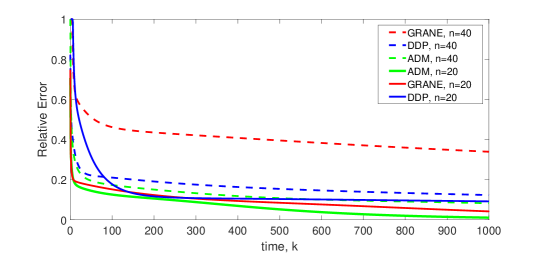
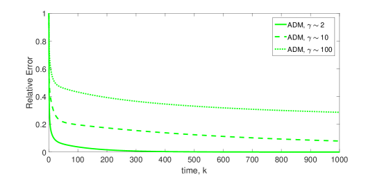
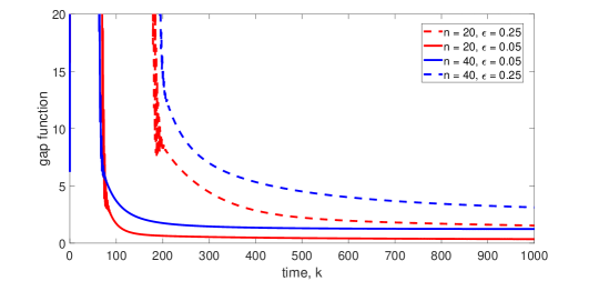
Figure 1: Comparison of the presented accelerated direct method (ADM) with GRANE and DDP.Figure 2: ADM in games with different condition numbers.Figure 3: ADM in merely monotone games.
Let us consider a class of games with monotone pseudo-gradients. Specifically, we have players and each player ’s objective is to minimize the cost function , where and . The local cost function is dependent on actions of all players, and the underlying communication graph is a randomly generated tree graph.
First, we randomly select , , and for all possible and to guarantee strong monotonicity of the pseudo-gradient.
We simulate the proposed gradient play algorithm and compare its implementation with the implementations of the algorithm GRANE presented in [22] and direct distributed procedure (DDP) from [3, 19]. Figure 1 demonstrates the simulation results for games with (the dimension of the local action sets is equal to 2) and supports the theoretic conclusions formulated in Remark 4. Moreover, Figure 2 demonstrates the simulation result obtained by the ADM in strongly monotone games with players under different condition numbers . As expected, the method slows down once increases (see Corollary 2). The evaluations are presented in terms of relative error equal to , where the unique solution to the game is calculated by 20000 iterates of the centralized gradient play.
Next, we simulate the ADM in the case of merely monotone games. To obtain this setting we randomly generate the parameters , and , and set up the matrix of the corresponding affine pseudo-gradient to contain two equal rows. The final pseudo-gradient for implementation is . Figure 3 provides the implementation result for the calculated gap function at the averaged iterates (see (91)), given the setting of Corollary 1 with and , and (the dimension of the local action sets is equal to 2). As we can see, the convergence rate slows down as increases. This is in consistence with Corollary 1.
6 Conclusion
This work extends centralized operator extrapolation method presented in [5] to distributed settings in games with merely monotone and restricted strongly monotone pseudo-gradient mapping, where players can exchange their information only with local neighbors via some communication graph.
In merely monotone games, a sublinear rate is achieved for the value of the gap function. This is the first known result on the convergence rate analysis of distributed procedures applied to merely monotone games. In the case of restricted strongly monotone pseudo-gradient, the proposed procedure is proven to possess a geometric rate and to outperform the previously developed algorithms calculating Nash equilibria in games under the same assumptions. Future research directions include consideration of a more general communication topology and study of lower bounds for convergence rates of distributed methods in such class of games.
References
[1]
T. Alpcan and T. Başar.
Distributed Algorithms for Nash Equilibria of Flow
Control Games.
In Advances in Dynamic Games, pages 473–498. Springer, 2005.
[2]
M. Bianchi, G. Belgioioso, and S. Grammatico.
A distributed proximal-point algorithm for nash equilibrium seeking
under partial-decision information with geometric convergence.
arXiv preprint arXiv:1910.11613, 2019.
[3]
M. Bianchi, G. Belgioioso, and S. Grammatico.
A fully-distributed proximal-point algorithm for nash equilibrium
seeking with linear convergence rate.
In 2020 59th IEEE Conference on Decision and Control (CDC),
pages 2303–2308, 2020.
[4]
M. Bianchi and S. Grammatico.
Fully distributed nash equilibrium seeking over time-varying
communication networks with linear convergence rate.
IEEE Control Systems Letters, 5(2):499–504, 2021.
[5]
G. Kotsalis, G. Lan, and T. Li.
Simple and optimal methods for stochastic variational inequalities,
i: Operator extrapolation.
SIAM Journal on Optimization, 32(3):2041–2073, 2022.
[6]
G. Lan.
First-order and stochastic optimization methods for machine learning.
Springer, 2020.
[7]
G. Lan and Y. Zhou.
Random gradient extrapolation for distributed and stochastic
optimization.
SIAM Journal on Optimization, 28(4):2753–2782, 2018.
[8]
N. Li, Y. Yao, I. Kolmanovsky, E. Atkins, and A. R. Girard.
Game-theoretic modeling of multi-vehicle interactions at uncontrolled
intersections.
IEEE Transactions on Intelligent Transportation Systems,
23(2):1428–1442, 2022.
[9]
A. Nemirovski.
Prox-method with rate of convergence o(1/t) for variational
inequalities with lipschitz continuous monotone operators and smooth
convex-concave saddle point problems.
SIAM Journal on Optimization, 15(1):229–251, 2004.
[10]
Yu. Nesterov and L. Scrimali.
Solving strongly monotone variational and quasi-variational
inequalities.
Discrete and Continuous Dynamical Systems - A,
31(4):1383–1396, 2011.
[11]
D.T.A. Nguyen, D.T. Nguyen, and A. Nedić.
Distributed nash equilibrium seeking over time-varying directed
communication networks.
IEEE Transactions on Control of Network Systems, pages 1–12,
2025.
[12]
A. Olshevsky and J. Tsitsiklis.
Convergence speed in distributed consensus and averaging.
SIAM Journal on Control and Optimization, 48(1):33–55, 2009.
[13]
J.-S. Pang and F. Facchinei.
Finite-dimensional variational inequalities and complementarity
problems : vol. 1.
Springer series in operations research. Springer, New York, Berlin,
Heidelberg, 2003.
[14]
G. Qu and N. Li.
Accelerated distributed Nesterov gradient descent.
IEEE Transactions on Automatic Control, 65(6):2566–2581, 2020.
[15]
W. Saad, H. Zhu, H. V. Poor, and T. Başar.
Game-theoretic methods for the smart grid: An overview of microgrid
systems, demand-side management, and smart grid communications.
IEEE Signal Processing Magazine, 29(5):86–105, 2012.
[16]
G. Scutari, S. Barbarossa, and D. P. Palomar.
Potential games: A framework for vector power control problems with
coupled constraints.
In 2006 IEEE International Conference on Acoustics Speech and
Signal Processing Proceedings, volume 4, pages 241–244, May 2006.
[17]
M. Sedlmayer, D.-K. Nguyen, and R. I. Bot.
A fast optimistic method for monotone variational inequalities.
In Andreas Krause, Emma Brunskill, Kyunghyun Cho, Barbara Engelhardt,
Sivan Sabato, and Jonathan Scarlett, editors, Proceedings of the 40th
International Conference on Machine Learning, volume 202 of Proceedings
of Machine Learning Research, pages 30406–30438. PMLR, 23–29 Jul 2023.
[18]
W. Shi, Q. Ling, G. Wu, and W. Yin.
EXTRA: An Exact First-Order Algorithm for Decentralized
Consensus Optimization.
SIAM Journal on Optimization, 25(2):944–966, 2015.
[19]
T. Tatarenko and A. Nedić.
Geometric convergence of distributed gradient play in games with
unconstrained action sets.
IFAC-PapersOnLine, 53(2):3367–3372, 2020.
21st IFAC World Congress.
[20]
T. Tatarenko and A. Nedić.
Accelerating distributed nash equilibrium seeking.
In 2024 European Control Conference (ECC), pages 323–328,
2024.
[21]
T. Tatarenko, W. Shi, and A. Nedić.
Accelerated gradient play algorithm for distributed nash equilibrium
seeking.
In 2018 IEEE Conference on Decision and Control (CDC), pages
3561–3566, 2018.
[22]
T. Tatarenko, W. Shi, and A. Nedić.
Geometric convergence of gradient play algorithms for distributed
nash equilibrium seeking.
IEEE Transactions on Automatic Control, 66(11):5342–5353,
2021.
[23]
M. Ye, Q.-L. Han, L. Ding, and S. Xu.
Distributed nash equilibrium seeking in games with partial decision
information: A survey.
Proceedings of the IEEE, 111(2):140–157, 2023.
Since , , , we get
for all .
Moreover, as , the inequality holds for all . Indeed, given that , we obtain
where the last inequality follows from the fact that
as is an increasing function in for , whereas for and .
To obtain (92), we notice that under the choice of , one can conclude that
whereas
(113)
Since , there exists such that for any . The inequality holds for any sufficiently large () as .
Finally, , which converges to as . Thus, there exists such that for , as decreases monotonically to 0 as . By taking we obtain (92).