The evolution of a supermassive binary black hole in an non-spherical nuclear star cluster

Abstract

In this Paper we consider a secular orbital evolution of a supermassive binary black hole (SBBH) with unequal masses $M_{p}$ and $M_{s}<M_{p}$ immersed in a central part of a non-spherical nuclear star cluster (NSC). When the mass of NSC enclosed inside the orbit becomes smaller than $M_{s}$ dynamical friction becomes inefficient. The subsequent orbital evolution of SBBH is largely governed by perturbing tidal potential of NSC arising from its non-sphericity. When the perturbing potential is mainly determined by quadrupole harmonics with azimuthal number $|m|=2$ the corresponding secular dynamics of the SBBH does not conserve any components of the angular momentum and can lead, for this reason, to the formation of highly eccentric orbits. Then such orbits can experience an efficient circularization due to emission of gravitational waves (GW). In this Paper we consider this situation in some detail.

We study analytically the secular evolution taking into account the important effect of Einstein apsidal precession and estimate the largest possible value of $e$, which can be obtained. We confirm and extend our analytic results by solving numerically the secular equations.

These results are used to estimate a possibility of fast orbital circularization through emission of gravitation waves on a highly eccentric orbit, with circularization timescale of the order of the orbital period. We find that our mechanism could result in such events on a time scale of the order of or smaller than a few Gyr. It is stressed that for particular values of the model parameters such events may sometimes be distinguished from the ones expected in more standard scenarios, since in our case the eccentricity may remain substantial all the way down to the final merger.

It is also noted that our results can be applied to other astrophysical settings, e.g. to study the orbital evolution of a binary star or a proto planetary system inside a massive deformed gas cloud.

I Introduction

The possibility that supermassive binary black holes (SBBHs) may harbor in centers of many galaxies is a natural consequence of the process of galaxy mergers and the subsequent evolution of two gravitationally unbound black holes toward the center of mass of the newly formed galaxy due to dynamical friction. The idea of the existence of such objects was put forward in several papers; see, for example, [1] and [2] and was explored later by numerous researchers; see e.g. [3] for a review of the appropriate theoretical aspects and [4] for a review of potential candidates found in observations (see also [5]). In particular, SBBHs may manifest themselves as sources of various nonstandard activity in galactic centers, with perhaps the most well known example being the explanation of the quasi-periodic outbursts observed in the quasar OJ 287. [6]. Even more importantly, SBBHs may provide the most powerful sources for future space-based gravitational wave antennas, see, e.g. [8] and [9], [10] for a more recent review.

It was pointed out in [2] that when a SBBH becomes gravitationally bound its orbital evolution may be so slow that the formation of the sources of gravitational waves could be impossible for cosmological, i.e. Hubble, time. This problem was nicknamed as ’the final parsec problem’. Over the years several possible solutions to the final parsec problem were proposed, such as e.g. the interaction of SBBH with gaseous environment (e.g. in the form of an accretion disk, see [11], and also [12] for a recent discussion and references), or triple systems of supermassive black holes, see e.g. [13] and [14], or the possibility of the central stellar population to have a non-spherical distribution. We consider below the latter possibility in some detail.

A non-spherical shape of the central regions of a galaxy may alleviate the central parsec problem in two ways. At first, it leads to a larger bulk of stars able to gravitationally interact with SBBH due to non-conservation of the absolute values of their angular momenta, thus facilitating the process of hardening of a gravitationally bound supermassive binary, see [15]. Secondly, since the angular momentum of the binary is also not conserved its orbital evolution could lead, in principle, to the formation of eccentric orbits in a way analogous to the well known von Zeipel-Lidov- Kozai effect [16], [17] and [18], hereafter ZLK, see [19] for a detailed historical review of these studies. If periastron of such eccentric orbits is small enough the emission of gravitational waves can lead to an efficient loss of orbital energy with the subsequent merger of the black holes in a time, smaller than the Hubble time.

So far, the problem of SBBHs evolution in the central parts of a non-spherical galaxy has been mainly treated by numerical calculations. However, since the numerical approach confronts significant difficulties, some additional simplification have been used in these numerical studies. In particular, in certain papers the authors assumed that SBBH’s orbit is circular, see e.g. [20], or the stellar distribution is either spherically symmetric, see e.g. [21] and [22] and references therein, or axially symmetric, see e.g.[23], [24], [25] and [26]. The models with broken axial symmetry usually implied that stellar density is uniform on triaxial elliptical shells, see e.g. [27] and [28]. All these symmetries are likely to be absent in a realistic stellar environment of SBBH .

In this Paper we would like to analyze the evolution of SBBH binary consisting of a more massive black hole (a primary) with mass $M_{p}$ surrounded by a nuclear star cluster (NSC) and a less massive intruding black hole (a secondary) with mass $M_{s}\ll M_{p}$. The star cluster is assumed to have a non-spherical distribution of stellar density at the scales of order of the radius of influence of the primary, $r_{infl}$, which may provide a perturbation to the gravitational potential of the primary at much smaller scales. Note that, in order to have a non-trivial perturbation of gravitational potential the distribution of stellar density shouldn’t be uniform on elliptical shells, since it is well known that gravitational potential inside such a shell is uniform, see e.g. [30]. Therefore, we are going to make the essential assumption that the stellar distribution deviate significantly from being uniform on the elliptical shells, although its exact form is not important for our purposes. After this assumption is made the non-spherical part of gravitational potential may cause a secular orbital evolution at scales smaller than $r_{infl}$. In case when the stellar distribution is non-spherical only at scales $\sim r_{infl}$, at much smaller scale the radial dependence of the perturbing gravitational potential, $V_{p}$ in the quadrupole (or, tidal) approximation is quadratic, while its angular dependence is proportional to a linear combination of spherical harmonics of the degree $l=2$ with the azimuthal number $m$ ranging from $-2$ to $2$,

$$V_{c}\propto r^{2}\sum_{m=-2}^{2}\alpha_{m}Y_{2,m}(\theta,\phi),$$ (1)

where $\theta$ and $\phi$ are polar and azimuthal angles in spherical coordinate system. The requirement that the gravitational potential is real links the terms with negative and positive $m$ by the requirement that $\alpha_{-m}=(-1)^{m}{\alpha_{m}}^{*}$, where $(^{*})$ stands for complex conjugate. Therefore, the angular dependence can be characterized by only positive values of $m$. Moreover, by a rotation of coordinate system the terms with $m=1$ can be eliminated, see e.g. [31] for the corresponding expressions. Thus, a general non-uniform distribution of stellar density leads to the presence of terms proportional to the spherical harmonics with $m=0$ and $m=2$ as well as their complex conjugate .

Thus, we expect that at scales $\ll r_{infl}$ the orbital dynamics is mainly governed by the Newtonian potential of the primary and the influence of the non-spherical distribution of stars as well as other factors (e.g. the relativistic corrections to the Newtonian potential, gravitational potential of stars within the orbit, etc.). This influence can be treated as perturbing corrections that cause a secular evolution of the orbit. On the other hand, dynamical friction is expected to be efficient only when a typical stellar mass enclosed within the binary orbit, $M_{st}$, is larger than the mass of the secondary black hole, and becomes inefficient at scales smaller than the the scale $r_{df}$ corresponding to the condition $M_{st}(r_{df})=M_{s}$, see [33] and [22]. In our case $M_{s}\ll M_{p}$, therefore, the scale $r_{df}$ should be smaller than $r_{infl}$, and therefore the secular evolution appears to be important precisely at the scales, where the orbital evolution due to dynamical friction is expected to stall.

The term in the perturbing potential determined by the azimuthal number $m=0$ is axially symmetric. Its presence leads to the secular evolution of the ZLK type. This evolution has been studied by many authors (see, e.g. [33] for a simple approach in a similar setting). Since the axial symmetry implies that the projection of orbital angular momentum onto the axis perpendicular to the symmetry plane is conserved, the secular evolution of eccentricity due to this term is limited by this conservation law. On the other hand, the secular evolution that arises from the presence of the term determined by $m=2$ does not conserve any component of angular momentum. Its presence can lead, in principle, to a secular evolution, which can bring initially small or moderate eccentricity to values close to unity. A binary with a highly eccentric orbit can evolve very fast due to the emission of gravitational waves. The purpose of this paper is to consider such a possibility using analytic and semi-analytic methods. We also will give some order of magnitude estimates, which may be appropriate for some interesting astrophysical objects.

To the best of our knowledge, such a problem has not been considered in the context of secular orbital evolution of SBBHs However, it has been considered by several authors in the context of secular evolution of stellar mass binaries orbiting in a star cluster, see e.g [34], [35], [36] and [37]. To formulate Hamiltonian describing the secular dynamics of orbital elements due the presence of non-spherical stellar distribution we use the averaged over the mean anomaly expression for the perturbing potential obtained in [35].

Since, in general, equations describing the secular evolution determined by the $m=2$ terms cannot be integrated analytically even in the simplest case when the primary gravitational potential is Newtonian and all other perturbing factors are neglected, we are going to make a number of rather drastic assumptions to make our problem analytically treatable. At first, we formally assume that all stars in the vicinity of the secondary are quickly dispersed and neglect their gravitational field. Secondly, we mainly concentrate on the dynamics determined by the $m=2$ terms and only briefly discuss effects arising from the additional inclusion of the $m=0$ term. Thirdly, we formally assume in our analytic study that there is a stage in the evolution of the dynamical system when both eccentricity $e_{0}$ and inclination to the plane of symmetry $i_{0}$ are small. This assumption allows us to find some approximate analytic solutions. Fourthly, we neglect all relativistic corrections apart from the effect of Einstein precession of the apsidal line, which is treated as a perturbation leading to a slow evolution of the parameters describing our approximate analytic solutions obtained for the purely Newtonian problem.

We find that the system exhibit quasi-periodic behavior with quasi-periodic cycles with periods order of the characteristic time of the ZLK effect. In the limit $i_{0}\rightarrow 0$, during half of the period the inclination $i$ is close to zero and it is close to $\pi$ during another half. These stages are separated by relatively short time intervals of growth or decrease of the inclination. These time intervals tend to zero when $i_{0}\rightarrow 0$. Twice per cycle the value of inclination passes through $\pi/2$, the first time when the inclination increases from $0$ to $\pi$, and the second time on its way back. The eccentricity $e$ also reaches its maximal values twice per cycle, at times close to the times corresponding to inclination being equal to $\pi/2$. The maximal values are inversely proportional to $i_{0}$. They also turn out to be functions of $\omega_{0}$ - the nodal angle at the moment of time when inclination and eccentricity have their minimal values per cycle, $e=e_{0}$ and $i=i_{0}$.

Corrections resulting from next order terms in the expansion over $i_{0}$ and $e_{0}$ in the equations of motions as well as from other factors such as the Einstein precession lead to a slow change of $i_{0}$, $\omega_{0}$ and $e_{0}$. As a results of it the maximal values of $e$ can be very close to unity at a time much larger than the cycle period (say, one hundred times larger, see below). In case when the slow evolution is determined by the Einstein precession, arguments based on the conservation of full Hamiltonian of the problem lead to an estimate of the maximal possible value of eccentricity, which turns out to the proportional to the rate of Einstein precession.

The analytic results provide some important qualitative understanding of the general dynamics of the system, but, they are directly applicable only when $i_{0}$ is quite small. Since a number of binaries with a small $i_{0}$ is expected to be quite small, the direct application of the analytic results of the problems of a rapid circularization due to emission of gravitational waves (hereafter, GWs) gives a small number of such events. We show, however, using numerical means, that systems with rather large initial inclinations can also experience a similar dynamics. This is partly explained by the observation that even in this case when the system evolves during a sufficiently long time there are extended periods, which correspond to the cycles with rather small minimal inclinations and, accordingly, rather large maximal values of eccentricity.

These results are used to estimate the possibility of an efficient circularization due to emission of GWs. The efficient circularization is defined as having the characteristic circularization timescale being order of or smaller than the orbital period. In our estimates we use an empirical relationship between NSC size and a mass of the central black hole reported in [38] for early type galaxies under the assumption that $r_{infl}$ has the same order of magnitude as the NSC size, see also [38]. We also assume that the stellar density distribution inside NSC has the standard Young profile [39]. We show that in our model the efficient circularization is expected at times order of or smaller than a few Gyrs provided that the mass ratio of SBBH, $q$, is sufficiently large, $q>\sim 0.04$. It is important to point out that, for certain parameters of the problem, orbital periastron in the beginning of the circularization phase is estimated to be as small as a few gravitational radii. That means that, in this case, the orbital eccentricity remains to be relatively larger all the way down to the black holes merger. This would allow one to distinguish GW events originating from our mechanism from the ones related to the standard hardening process by a different shape of GW signal. This also may be relevant for the formation of binaries with the parameters similar to the ones assumed in the standard model of OJ 287.

The plan of the Paper is as follows 1) In Section 2 we introduce equations of motion describing the secular evolution of SBBHs orbit due to the action of the perturbing potential and the Einstein apsidal precession.

2) In Section 3 we provide the asymptotic solution of the equations of motion in the purely Newtonian case, taking into account only the $m=2$ terms in the perturbing potential. We also provide some brief numerical analysis of the role of the $m=0$ term and argue that it shouldn’t change qualitatively the behavior of the system if its contribution is relatively small in Appendix A.

3)In Section 4 we analyze the role of Einstein precession and estimate the maximal value of eccentricity, which could be reached in the course of SBBH evolution. It is shown that its role can be described as a map between parameters of consequent cycles of the Newtonian secular evolution and a technical analysis of this map is made in Appendix B. We also provide some numerical analysis, which is used to justify our assumption that our analytic results are applicable to sufficiently large inclinations $i_{0}$ when a sufficiently large enough evolution time is considered.

4) In Section 5 we estimate parameters of SBBHs and NSCs required for efficient orbital circularization due to GWs emission.

We conclude that relatively large mass ratios $q>\sim 0.04$ are preferable. We also provide an upper estimate of a typical time elapsed before such circularization takes place.

5) We summarize and finally discuss our results in Section 6.

Note that a reader who is interested in astrophysical applications only can omit Section 2-4 and go directly to Section 5, which is written in a self-consistent way.

II The secular evolution of SBBHs in the presence of quadrupole perturbing potential

Let us consider the orbit of the secondary black hole with mass $M_{s}$ in gravitational potential $V=V_{p}+V_{c}$, where $V_{p}$ is the gravitational potential of the primary black hole with mass $M_{p}$ and $V_{c}\ll V_{p}$ is a perturbing potential generated by the outer parts of the stellar cluster with a non-symmetric distribution of stellar mass density. Let us start for simplicity from Newtonian approximation, when $V_{p}=GM_{p}/r$ (general relativistic corrections will be considered below). As have already been discussed in Introduction we assume in this Paper that $V_{c}$ has the quadrupole form. Under this assumption in Cartesian coordinate system $(x,y,z)$, $V_{c}$ of the form (1) can be represented as:

$$V_{c}=\Omega^{2}[\sin\nu(2z^{2}-(x^{2}+y^{2}))+\cos\nu(x^{2}-y^{2})],$$ (2)

where the constant $\nu$ determines therelative contribution of the two terms in square brackets, $\Omega$ has the dimension of inverse time, it is assumed to be smaller than mean motion

$$n_{0}=\Omega\ll\sqrt{GM_{p}\over a^{3}},$$ (3)

where $a$ is the semi-major axis of the secondary black hole orbit. The first term in square brackets in (2) is determined by the harmonics of the potential with azimuthal number $m=0$. It has, accordingly, the azimuthal symmetry, which conserves the projection of orbital angular momentum onto the axis $z$. It can be shown (see e.g. [35]), that the secular evolution due to the presence of this term has the standard ZLK character. The second term is due to non-axially symmetric part of the potential, which is determined by harmonics with $m=\pm 2$. It leads to a non-standard secular evolution, which does not conserve any component of orbital angular momentum.

We parametrize the orbit by the standard set of variables including orbital semi-major axis $a$, eccentricity $e$, inclination $i$, mean motion $n_{0}$, argument of pericentre $\varpi$ and longitude of ascending node $\omega$ . In order to bring equations of motion to the canonical form one can use Delaunay variables (see for example [41])

$$P_{1}=\sqrt{GMa},\quad P_{2}=\sqrt{(1-e^{2})}P_{1},\quad P_{3}=\cos iP_{2},$$ (4)

which are generalized momenta canonically conjugate to $n_{0}$, $\varpi$ and $\omega$, respectively.

We use the average of (2) over the mean anomaly $n_{0}t$ using equations (A1-A3) from [35], the resulting expression is

$$H=\Omega^{2}[\sin\nu(2<z>^{2}-(<x>^{2}+<y>^{2})+\cos\nu(<x>^{2}-<y>^{2})],$$ (5)

where $<..>$ stand for the averaged quantities, provides Hamiltonian for the secular motion.

The corresponding equations of motion follow from Hamilton equations and have the form

$${de\over dt}={\epsilon\over P_{1}e}{\partial\over\partial\varpi}H,\quad{di\over dt}={1\over P_{1}\epsilon\sin i}({\partial\over\partial\omega}-\cos i{\partial\over\partial\varpi})H,$$

$${d\varpi\over dt}=-{1\over P_{1}\epsilon}(\cos i{\partial\over\partial\cos i}+{\epsilon^{2}\over e}{\partial\over\partial e})H,\quad\quad{d\omega\over dt}={1\over P_{1}\epsilon}{\partial\over\partial\cos i}H,$$ (6)

where $\epsilon=\sqrt{1-e^{2}}$ and we note that, since the problem is stationary, the orbital energy and, accordingly, semi-major axis $a$ and $P_{1}$ are conserved. It is convenient to divide the full Hamiltonian $H$ into two parts $H=\sin\nu H_{0}+\cos\nu H_{2}$, where $H_{0}$ and $H_{2}$ are proportional to $2<z>^{2}-(<x>^{2}+<y>^{2})$ and $<x>^{2}-<y>^{2}$), respectively. We also represent time derivatives of all our dynamical variables as the sums

$${dq\over dt}=\nu_{o}({dq\over dt})_{0}+\nu_{2}({dq\over dt})_{2},$$ (7)

where $q$ stands for any of $e$, $i$, $\omega$ and $\varpi$, $({dq\over dt})_{0}$ and $({dq\over dt})_{2}$ are given by eqns (6) when $H$ in these equations is replaced by $H_{0}$ and $H_{2}$, respectively.

From the results reported in [35] we obtain

$$H_{0}={\Omega^{2}a^{2}\over 4}h_{0},\quad h_{0}=((2+3e^{2})(1-3\cos^{2}i)-15e^{2}\sin^{2}i\cos 2\varpi),$$ (8)

and

$$H_{2}={\Omega^{2}a^{2}\over 4}h_{2},\quad h_{2}=(\cos^{2}i\cos 2\omega(5e^{2}\cos 2\varpi-(2+3e^{2}))$$

$$-10e^{2}\cos i\sin 2\omega\sin 2\varpi$$

$$+\cos 2\omega(5e^{2}\cos 2\varpi+2+3e^{2})).$$ (9)

We obtain from eq. (8)

$$({de\over d\tau})_{0}=30\epsilon e\sin^{2}i\sin 2\varpi$$

$$({di\over d\tau})_{0}=-{30e^{2}\over\epsilon}\sin i\cos i\sin 2\varpi$$

$$({d\varpi\over d\tau})_{0}=-{6\over\epsilon}(5\cos^{2}i(\cos 2\varpi-1)+\epsilon^{2}(1-5\cos 2\varpi))$$

$$({d\omega\over d\tau})_{0}={6\over\epsilon}(5e^{2}\cos 2\varpi-(2+3e^{2})),$$ (10)

where

$$\tau=t/t_{*},\quad t_{*}={4n_{0}\over\Omega^{2}},\quad n_{0}={\sqrt{GM_{p}\over a^{3}}.}$$ (11)

Eqns (10) describe the standard ZLK evolution (see e.g. [33], hereafter IPS). To see this, it is enough to make a simple replacement of variables in (10), namely, replace $\tau$ with $t=t_{*}\tau$. From eq. (9) we have

$$({de\over d\tau})_{2}=-10\epsilon e(\cos 2\omega\sin 2\varpi(1+\cos^{2}i)+2\cos i\sin 2\omega\cos 2\varpi)$$ (12)

$$({di\over d\tau})_{2}=-{2\sin i\over\epsilon}(5e^{2}\cos i\cos 2\omega\sin 2\varpi+\sin 2\omega(5e^{2}\cos 2\varpi+2+3e^{2}))$$ (13)

$$({d\varpi\over d\tau})_{2}=-{2\over\epsilon}(\cos 2\omega(5\cos 2\varpi(\epsilon^{2}+\cos^{2}i)+3\epsilon^{2}-5\cos^{2}i)-5(2-e^{2})\cos i\sin 2\omega\sin 2\varpi)$$ (14)

$$({d\omega\over d\tau})_{2}={2\over\epsilon}(\cos i\cos 2\omega(5e^{2}\cos 2\varpi-(2+3e^{2}))-5e^{2}\sin 2\omega\sin 2\varpi).$$ (15)

Since we consider a binary black hole, we need to take into account relativistic corrections to the Newtonian motion. Since the orbital semi-major axis is much larger than the gravitational radius of the central (i.e. primary) black hole, it is enough for our purposes to take into account the first-order correction, which is the Einstein precession of the apsidal angle. This rate is given by the standard expression, see for example [42]

$${\dot{\varpi}_{E}}={3GM\over c^{2}a(1-e^{2})}n_{0}.$$ (16)

where $c$ is the speed of light. In terms of $\tau$ (see eq. (11) eq. (16) can be rewritten as

$${d\varpi_{E}\over d\tau}=\beta_{E}\epsilon^{-2},\quad\beta_{E}={12GM\over c^{2}a}{n_{0}^{2}\over\Omega^{2}},$$ (17)

where $\epsilon$ is defined after eq.(6). It is possible to see that the corresponding contribution to Hamiltonian of our system has the form

$$H_{E}={\Omega^{2}a^{2}\over 4}h_{E},\quad h_{E}=-{\beta_{E}\over\epsilon}.$$ (18)

Note that, in principle, it is easy to incorporate in our dynamical system the next order relativistic correction due to the Lense-Thirring precession of the nodal angle. The corresponding precession rate of this angle, $\dot{\omega}_{LT}$, is proportional to the primary black hole rotational parameter $\chi$ (such that $|\chi|<1$). Its explicit expression can be found in e.g. [43]:

$$\dot{\omega}_{LT}={2\chi G^{2}M^{2}\over c^{3}\epsilon^{3}a^{3}}.$$ (19)

From the condition $|\dot{\omega}_{LT}|<\dot{\varpi}_{E}$ we readily find

$${GM(1+e)\over c^{2}r_{p}}<{9\over 4}{1\over|\chi|^{2}},$$ (20)

where $r_{p}=(1-e)a$ is the orbital periastron. It is shown below that our dynamical system experiences secular changes of eccentricity between a state, where $e$ is small and ${GM\over c^{2}r_{p}}\ll 1$ and a state, where $e$ is close to unity. But, even for the latter state ${GM\over c^{2}r_{p}}$ is expected to be smaller than ${1\over 4}$, see eq. (69) below. Thus, the inequality (20) is satisfied for all potentially interesting states of the system, and, therefore, for simplicity, we neglect the evolution of the nodal angle caused to the Lense-Thirring effect below.

Accordingly, the full Hamiltonian of our dynamical system, $H$, can be represented as

$$H={\Omega^{2}a^{2}\over 4}h,\quad h=(\sin(\nu)h_{0}+\cos(\nu)h_{2})+h_{E}.$$ (21)

The full equations of motion following from (21) have symbolic form analogous to (7)

$${dq\over d\tau}=\sin\nu({dq\over d\tau})_{0}+\cos\nu({dq\over d\tau})_{2}+({dq\over d\tau})_{E},$$ (22)

where by $({dq\over d\tau})_{E}$ we imply that (17) should be added to the equation describing the rate of apsidal precession.

III Numerical and asymptotic analytic solutions of the secular equations in the Newtonian approximation

Since in this Paper we would like to discuss only a qualitative character of the evolution of the binary under the influence of the perturbing potential and a principal possibility of the gravitational capture of the secondary BH on close-in orbits, we are going to make a number of rather drastic simplifying assumptions. In particular, in this Section we consider a simplified model problem, where the potential is determined by only $\pm 2$ terms in equation (2) and the Einstein precession is negligible. We set, accordingly, $\nu=0$ and $({dq\over d\tau})_{E}={d\varpi_{E}\over d\tau}=0$ in eq. (22) However, we briefly discuss effects originating from $\nu\neq 0$ in Appendix A. In this case the secular evolution is determined by equations (12-15).

III.1 The asymptotic numerical solution in the limit $i_{0}\rightarrow 0$

A typical example of the numerical solution is illustrated in Fig. 1, where we show the solution corresponding to small initial eccentricity $e_{0}=0.1$, and two small values of initial inclination $i=0.01$ (solid lines) and $i=0.1$ (dashed lines), respectively. The top panel shows the evolution of $e$ and $i$ as the black and red curves, respectively, while the bottom panel describes the evolution of $\omega$ and $\varpi$. For this purpose, we find it convenient to introduce a new angle, $\alpha$, defined according to the rule: $\alpha=2(\omega+\varpi)$ when $i<\pi/2$ and $\alpha=2(\omega-\varpi)$ when $i>\pi/2$. We show the evolution of $\sin(\alpha)$ as the black curves and $\cos(\alpha)$ as the red curves.

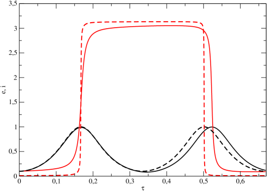
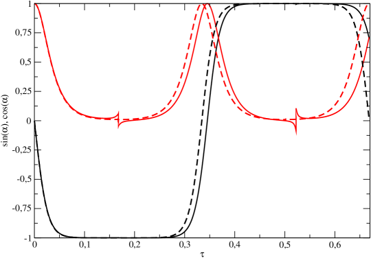
Figure 1: Top panel. The numerical dependencies of $e$ (the black curves) and $i$ (the red curves) as functions of time, the initial value of eccentricity, apsidal and nodal angles, $e_{0}=0.1$, $\varpi_{0}=2\pi/5$ and $\omega_{0}=-\varpi_{0}=-2\pi/5$, respectively. Note that the particular values of $\varpi_{0}$ and $\omega_{0}$ are chosen for illustrative purpose only, we checked that other values result in a similar evolution. Also note that the condition $\alpha_{0}=2(\omega_{0}+\varpi_{0})=0$ ensures that the initial value of eccentricity is the minimal one in the course of evolution. Solid and dashed curves correspond to initial inclination $i_{0}=0.1$ and $0.01$, respectively. Bottom panel. The evolution of $\sin(\alpha)$ (the black curves) and $\cos(\alpha)$ (the red curves), the initial values of the state variables and types of the curves are the same as in top panel.

One can see from Fig. 1 that the evolution of $e$ is almost periodical with the eccentricity gradually increasing from the initial small value to a value $e\approx 1$, then decreasing back to approximately the same minimal value; then this cycle repeats. On the other hand, $i$ during an extended initial period of time has small values, then it sharply grows to a value approximately equal to $\pi$, then it stays approximately constant again, then it sharply drops to small values and approaches values close to $i_{0}$ at the end of the calculation. Thus, we have approximately two periods of evolution of $e$ and one period of evolution of $i$ during computational time. It is very important to note that the fast time evolution of $i$ from $\sim 0$ to $\sim\pi$ and back occurs during time periods corresponding to $e\sim 1$, with its typical time duration decreasing with decreasing $i_{0}$. Apart from these time periods the curves corresponding to the different values of $i_{0}$ are close to each other. The curves showing the evolution of $\sin(\alpha)$ and $\cos(\alpha)$ are also quasi-periodic. Also, apart from a small ’kink-like’ feature seen in the curve describing the evolution of $\cos(\alpha)$ when it is close to zero these quantities smoothly transit through the time periods of the fast evolution of $i$. We have $\sin(\alpha)\approx-1$ and $\cos(\alpha)\approx 0$ when $i$ transits from $\sim 0$ to $\sim\pi$ and $\sin(\alpha)\approx 1$ and $\cos(\alpha)\approx 0$ when $i$ transits from $\sim\pi$ to $\sim 0$. Note that $\sin(\alpha)$ changes its sign approximately in the middle of the shown period of time, when $i\approx\pi$ and $e\approx e_{0}$.

These numerical results suggests the following analytical scheme for a treatment of the case with small initial values of eccentricity and inclination. At first, we consider the limit $i_{0}\rightarrow 0$ . In this case the numerical results indicate that the evolution can be considered as consisting of subsequent stages with $i\approx 0$ and $i\approx\pi$, respectively, with sharp jumps of $i$ between them and the duration of these jumps tends to zero when $i_{0}\rightarrow 0$. In contrast, in the same limit $i_{0}\rightarrow 0$ $\alpha$ is nearly a constant during the fast evolution of $i$. This behavior of $i$ can be used to construct an analytic asymptotic solution to equations (12) and (14-15).

III.2 The asymptotic analytical solution in the limit $i_{0}\rightarrow 0$

It is then turns out to be possible to consider a finite, but small $i_{0}$, and describe analytically the evolution within the region of sharp jumps using the simplifying assumptions that $e\sim 1$, $\cos(\alpha)\approx 0$ and $\sin(\alpha)\approx\mp 1$ during these special periods of time. Here we would like to consider a model problem, which provides a zero-order approximation to the asymptotic solution of our dynamical equations in the limit $i_{0}\rightarrow 0$. We start with some initial values of $e_{0}\ll 1$, $\omega_{0}$ and $\varpi_{0}$ and assume that the inclination angle $i=0$ until we reach the state with $e=1$ at some time $\tau=\tau_{*}$, which is expected to be finite. We then set $i=\pi$, $e=1$ and assume that the angle $\alpha$ is the same as it was in the end of the ppreceding stage. The eccentricity is expected to decrease to some minimal value, $e_{min}$, and then increase again to the state with $e=1$. The inclination angle is again switched to $i=0$ and the cycle is ended when $e$ reaches the value $e_{0}$. It follows from our previous discussion see equation (27), that in order to have $e_{min}=e_{0}$ we should have $\alpha=0$ and, accordingly, $\varpi_{0}=-\omega_{0}$. Thus, this model problem is characterized by two parameters, $e_{0}$ and $\omega_{0}$.

Setting $i=0$ and $\pi$ we have $\cos(i)=\pm 1$. It then follows from equations (12) and (14-15) that

$${de\over d\tau}=-20\epsilon e\sin 2(\varpi\pm\omega),$$ (23)

$${d(\varpi\pm\omega)\over d\tau}=-20\epsilon\cos 2(\varpi\pm\omega).$$ (24)

Additionally, from eq. (15) we obtain

$${d\omega\over d\tau}=\pm{2\over\epsilon}(5e^{2}\cos 2(\varpi\pm\omega)-(2+3e^{2})\cos 2\omega).$$ (25)

It is easy to see that eqns (23-24) can be also rewritten as

$${de\over d\tau}=\mp 20\epsilon e\sin\alpha,{d\alpha\over d\tau}=\mp 40\epsilon\cos\alpha.$$ (26)

Dividing (23) by (24) (or, the first eq. in (26) by the second one) we see that the quantity $C=e^{2}|\cos(\alpha)|$ is conserved. Note that the same conservation law follows from (9) when $i=0$ or $i=\pi$.

Since equations (23-24) form a complete set we can first solve them in all regions separately and then match all these solutions together keeping in mind that $e$ and $\alpha$ should be continuous during sharp jumps mentioned above. After that we can solve equation (25).

We assume that when $\tau=0$ the eccentricity $e$ is in its local minimum, $e=e_{0}$. Hence, as it follows from eq. (26) that $\alpha=0$ or $\pi$ when $\tau=0$, and, accordingly, $C=e_{0}^{2}$. It also follows from eqns (26) that they are invariant with respect to the change $\alpha\rightarrow\alpha+\pi$, $\tau\rightarrow-\tau$, and, therefore, the case $\alpha(\tau)=0$ and $\alpha(\tau=0)=\pi$ can be obtained from each other by the change of the sign of time. Therefore, we consider below only the case $\alpha(\tau=0)=0$. In this case we expect that $\cos(\alpha)>0$ in the course of the whole evolution and get $e^{2}_{0}=e^{2}\cos(\alpha)$. Using this relation we can express $\cos(\alpha)$ and $\sin(\alpha)$ in terms of $e$ as

$$\cos\alpha=({e_{0}\over e})^{2},\quad\sin\alpha=\kappa\sqrt{1-{({e_{0}\over e})}^{4}},$$ (27)

where $\kappa$ is equal to $\pm 1$ and the sign should be chosen from the following arguments. Initially, eccentricity should grow with time from $e_{0}$ to $1$. We also have $i=0$ initially, and, therefore, we should choose the sign $(+)$ in eq. (23). Thus, at the initial stage $\kappa$ should be equal to $-1$. After the state $e=1$ is reached we must choose the sign $(-)$ in eq. (23). Since $\alpha$ is assumed to pass continuously through the transition from one stage to another, $\kappa$ remains negative and the eccentricity, accordingly, decreases at times $\tau>\tau_{*}$. This happens until the state with $e=e_{0}$ is reached and the eccentricity must increase after the corresponding time. Therefore, we must change the sign of $\kappa$ and set $\kappa=1$ when $e=e_{0}$ at the stage with $i=\pi$. It is then follows from eq. (23) that the eccentricity increases again up to the state with $e=1$, we then change again $(-)$ to $(+)$ in eq. (23) after the corresponding time, while keeping $\kappa=1$. We have again the stage with $i=0$ after this moment of time, but with decreasing eccentricity. The eccentricity decreases down to $e=e_{0}$ and after the corresponding moment of time the cycle repeats.

Substituting eq. (27) in eq. (23) we formally obtain

$$\int^{e}_{e_{0}}{de\over e\epsilon\sqrt{1-{({e_{0}\over e})}^{4}}}=\mp 20\kappa\tau$$ (28)

Evaluation of the integral on l.h.s leads to a rather cumbersome expression. However, for our purposes it would enough to evaluate it only in the limit $e\gg e_{0}$. Let us consider, for definiteness, the initial stage with $i=1$ and $\kappa=-1$, where the expression on r.h.s. of (28) is positive. In this case we can divide the range of integration on two parts $e_{0}\leq e\leq e_{*}$ and $e_{*}\leq e\leq 1$, where an intermediate value of $e_{*}$ is chosen in such a way that $e_{0}\ll e_{*}\ll 1$. When considering the integral in the range $e_{0}\leq e\leq e_{*}$ we can set $\epsilon=1$, while in the range $e_{*}\leq e\leq 1$ we can set $\sqrt{1-{({e_{0}\over e})}^{4}}=1$ in the integrand. After these approximations are made the corresponding integrals are elementary. Moreover, their sum does not depend on $e_{*}$ in the leading order over $e_{0}/e_{*}$. In this way we obtain

$$\epsilon={(1-{e_{0}^{2}\over 8}\exp(40\tau))\over(1+{e_{0}^{2}\over 8}\exp(40\tau))},$$ (29)

and, from the condition $e(\tau_{*})=1$ we find that

$$\tau_{*}={1\over 40}\log{8\over e_{0}^{2}}.$$ (30)

The time $\tau_{*}$ is the characteristic time of the process under consideration and we consider in this Section the evolution of our system at times comparable to $\tau_{*}$.

When $\tau>\tau_{*}$ we should choose $(-)$ on r.h.s. of eq. (28) and specify the constant of integration in such a way that $e(\tau=\tau_{*})=1$. This branch of the solution corresponds to decreasing with time eccentricity and can be obtained from eq. (29) by changing $\tau$ to $2\tau_{*}-\tau$ due to symmetry arguments. It is clear that $e=e_{0}$ when $\tau=2\tau_{*}$. At this time we should change $\kappa$ from $-1$ to $1$, and at times $\tau>2\tau_{*}$ the solution possesses again growing eccentricity and can be obtained from eq. (28) by the substitution $\tau-2\tau_{*}$ instead of $\tau$. This branch describes the evolution of eccentricity until $\tau=3\tau_{*}$ when we have $e=1$ again. At this time we should again switch to the solution with decreasing eccentricity, which can be obtained in the same way as before, but changing $\tau$ in eq. (28) to $4\tau_{*}-\tau$. The latter branch describes the solution until $\tau=4\tau_{*}$. It is clear that the evolution of eccentricity is periodic with the period $2\tau_{*}$, but $\sin(\alpha)$ in eq. (27) is negative when $\tau<2\tau_{*}$ (or, $\kappa=-1$) and positive otherwise ($\kappa=1$). Thus, the whole period of the evolution of all state variables in the considered limit is $4\tau_{*}$. Using these rules we obtain explicitly

$$\epsilon={(1-{e_{0}^{2}\over 8}\exp(40\tau))\over(1+{e_{0}^{2}\over 8}\exp(40\tau))}\quad when\quad\tau<\tau_{*},$$

$$\epsilon={({e_{0}^{2}\over 8}\exp(40\tau)-1)\over(1+{e_{0}^{2}\over 8}\exp(40\tau))}\quad when\quad\tau_{*}<\tau<2\tau_{*},$$

$$\epsilon={(1-({e_{0}^{2}\over 8})^{3}\exp(40\tau))\over(1+({e_{0}^{2}\over 8})^{3}\exp(40\tau))}\quad when\quad 2\tau_{*}<\tau<3\tau_{*},$$

$$\epsilon={(({e_{0}^{2}\over 8})^{3}\exp(40\tau)-1)\over(1+({e_{0}^{2}\over 8})^{3}\exp(40\tau))}\quad when\quad 3\tau_{*}<\tau<4\tau_{*}.$$ (31)

Eqns (31) together with eq. (27), where we choose $\kappa=-1$ when $\tau<2\tau_{*}$ and $\kappa=1$ otherwise describe the whole cycle of the evolution of $e$ and $\alpha$ in the limit of an infinitesimally small initial inclination angle.

In order to describe the separate evolution of $\omega$ and $\varpi$ we should also solve eq. (25). Taking into account that the expression for $\cos(\alpha)$ in eq. (27) tells that the first term in the brackets in eq. (25) is equal to $5e_{0}^{2}$, which is small everywhere this term can be neglected. We then obtain from eq. (25)

$$\int_{\omega_{0}}^{\omega}{d\omega\over\cos(2\omega)}={1\over 10\kappa}\int^{e}_{e_{0}}{de(2+3e^{2})\over e\epsilon^{2}(1-{({e_{0}\over e})}^{4})},$$ (32)

where we use eq. (23) to change the integration variable from $\tau$ to $e$. We evaluate the integral on r.h.s. of eq. (32) in the same way as was done in the case of a similar integral in eq. (28). Note that in the case of eq. (32) there are only two branches corresponding to $\kappa=\mp 1$, which should be continuously joined together at $\tau=2\tau_{*}$. In this way we obtain

$$\sin(2\omega)={C^{-}_{\omega}\epsilon^{2}-e^{4/5}\over C^{-}_{\omega}\epsilon^{2}+e^{4/5}}\quad when\quad\tau<2\tau_{*},$$

$$\sin(2\omega)={C^{+}_{\omega}\epsilon^{-2}-e^{-4/5}\over C^{+}_{\omega}\epsilon^{-2}+e^{-4/5}}\quad when\quad 2\tau_{*}<\tau<4\tau_{*},$$ (33)

where

$$C^{-}_{\omega}={(1+\sin(2\omega_{0}))\over(1-\sin(2\omega_{0}))}e_{0}^{4/5}/(1-e_{0}^{2}),\quad C^{+}_{\omega}={(1+\sin(2\omega_{0}))\over(1-\sin(2\omega_{0}))}e_{0}^{-4/5}(1-e_{0}^{2}),$$ (34)

we use $C^{-}_{\omega}$ when $\tau<2\tau_{*}$ and $C^{+}_{\omega}$ is used otherwise. Sometimes it is convenient to redefine the angle $\omega$ according to the rule

$$\psi=\omega-{\pi\over 4},$$ (35)

and rewrite $C^{\kappa}$ as $C^{\mp}=e_{0}^{\pm 4/5}\cot^{2}\psi_{0}$, where $\psi_{0}=\psi(\tau=0)$. For our purposes we also need to know the dependency of $\cos(2\omega)$ on $e$, which can be obtained from eq. (33) and eq. (35)

$$\cos(2\omega)=-\sin(2\psi)=\mp{\sin(2\psi_{0})\over\sin^{2}(\psi_{0})}{e_{0}^{2/5}e^{2/5}\epsilon\over(C_{\omega}^{-}\epsilon^{2}+e^{4/5})}$$ (36)

when $\kappa=-1$ and

$$\cos(2\omega)=-\sin(2\psi)=\pm{\sin(2\psi_{0})\over\sin^{2}(\psi_{0})}{e_{0}^{-2/5}e^{-2/5}\epsilon^{-1}\over(C_{\omega}^{+}\epsilon^{-2}+e^{-4/5})}$$ (37)

in the opposite case. Note that the choice of sign agrees with the fact that $\cos(2\omega)$ should change its sign when $i$ transits from $0$ to $\pi$ and back. However, we stress that this behaviour is expected only in the Newtonian case and the sign can be unchanged when the Einstein apsidal precession is taken into account, as we discuss below. From the expressions (36) and (37) it follows that in the limit $e\rightarrow 1$ ($\epsilon\rightarrow 0$) we have

$$|\cos(2\omega)|\approx 2(C^{-}_{\omega})^{1/2}\epsilon,\quad|\cos(2\omega)|\approx 2(C^{+}_{\omega})^{-1/2}\epsilon.$$ (38)

We compare the analytic expressions (27), (31) and (33) in Fig. 2. One can see from this figure that there is a very good agreement between theoretical and numerical results apart from the regions, where $e\sim e_{0}$.

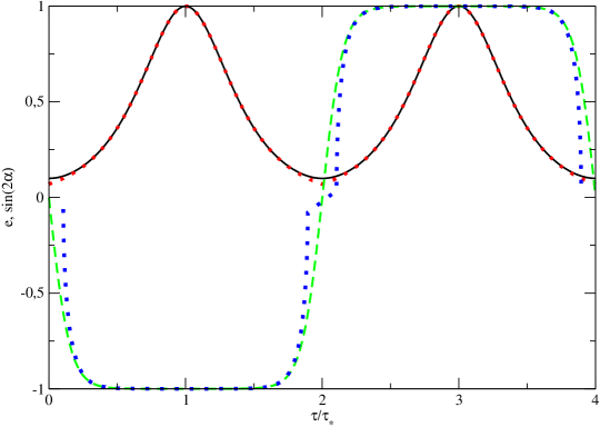
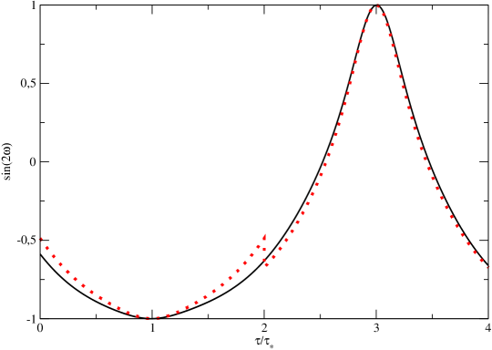
Figure 2: Top panel. The numerical dependencies of $e$ (solid line) and $\sin(2\alpha)$ (dashed line) as functions of time, the initial value of eccentricity, inclination angle, apsidal and nodal angles are $e_{0}=0.1$, $i_{0}=0.01$, $\varpi_{0}=2\pi/5$ and $\omega_{0}=-\varpi_{0}=-2\pi/5$, respectively. Dotted lines show the analytic expressions given by eqns (27) and (29). Note that, since it is expected that when $e\sim e_{0}$ our simple approach is invalid, the expression under the square root in (27) can be negative. The corresponding values of time are not shown. Bottom panel. The same as top panel, but for $\sin(2\omega)$. The solid and dotted curves represent the numerical result and the analytic expression (33), respectively.

III.2.1 The evolution of inclination in the linear regime

When the inclination $i$ is either small or close to $\pi$, we can use the solution described above to determine its evolution. For that we use eq. (13) setting there $\cos(i)=\pm 1$, and $\sin(i)=i_{+}$, where $i_{+}\equiv i$ when $i\ll 1$, or $\sin(i)=-i_{-}$, where $i_{-}=i-\pi$ when $i\approx\pi$, to obtain

$$i_{\pm}^{-1}{di_{\pm}\over d\tau}=-{2i\over\epsilon}(5e^{2}\sin(2(\varpi\pm\omega)\pm(2+3e^{2})\sin(2\omega))={e\over 2\epsilon^{2}}{de\over d\tau}\mp{2\over\epsilon}(2+3e^{2})\sin(2\omega)),$$ (39)

where we use eq. (23) to obtain the last equality. We use eq. (25) neglecting the first term in the brackets there to express the last term in (39) as $\tan(2\omega){d\omega\over d\tau}$. After this transformation is made the integration of eq. (39) is elementary with the result

$$i_{\pm}=C_{i}(\epsilon|\cos(2\omega)|)^{-{1\over 2}}.$$ (40)

In order to check eq. (40) we show the ratio $C_{i}/C_{i,0}$, where $C_{i}$ is evaluated for numerically calculated values of $i$, $e$ and $\omega$, and $C_{i,0}$ is a value of this quantity calculated for the initial values of these variables, $C_{i,0}\approx i_{0}\sqrt{|\cos(2\omega)|}$, in Fig. 3. One can see that $C_{i}$ is indeed close to a constant when $i$ is either close to zero or $\pi$. Moreover, when $i$ is close to $\pi$ the value of $C_{i}$ is close to the negative of its initial value.

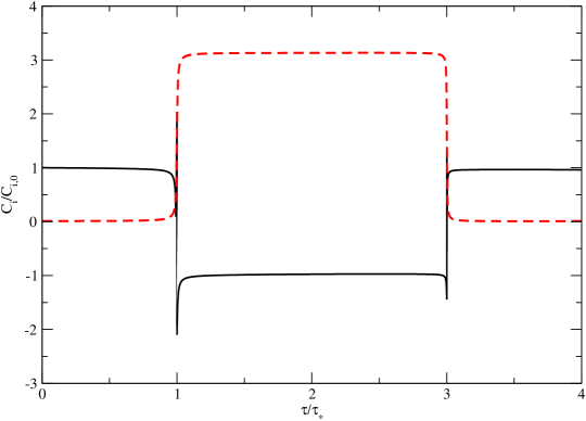
Figure 3: The dependencies of the ratio $C_{i}/C_{i,0}$ and $i$ on time shown as the solid line and dashed lines, respectively. The initial values of $i$, $e$ and $\omega$ are the same as the ones used in Fig. 2. To plot this Figure we use $i_{+}=i$ when $i\leq\pi/2$ and $i_{-}=i-\pi$ is used otherwise in eq. 40.

III.3 The evolution in the region of sharp jumps

As follows from our previous analysis when $\tau\approx\tau_{*}$ $e\approx 1$ and $i$ changes abruptly from $0$ to $\pi$, while when $\tau\approx 3\tau_{*}$ $e\approx 1$ again and we have the reverse abrupt change of $i$ from $\pi$ to $0$. From eqns (27) and (33) it is seen that we have $\cos\alpha\approx 0$, $\sin\alpha\approx-1$ and $\sin 2\omega\approx-1$, $\cos 2\omega\approx 0$ in the former case and $\cos\alpha\approx 0$, $\sin\alpha\approx 1$ and $\sin 2\omega\approx 1$, $\cos 2\omega\approx 0$ in the latter case. From these relations it is easy to see that we always have $\sin 2\varpi\approx 0$ and $\cos 2\varpi\approx 1$ in both cases. Therefore, when studying the evolution in the transition layers we can set $e=1$, $\sin 2\varpi=0$, $\cos 2\varpi=1$ and $\cos 2\omega\approx 0$, $\sin 2\omega\approx\kappa$ in r.h.s. of eqns (12) and (13) and change the time derivative of eccentricity in l.h.s of eq. (12) to the time derivative of $\epsilon=\sqrt{1-e^{2}}$ according to the rule ${de\over d\tau}\approx-\epsilon{d\epsilon\over d\tau}$. In this way we obtain

$${d\epsilon\over d\tau}=20\kappa\cos i,\quad{di\over d\tau}=-\kappa{20\sin i\over\epsilon}.$$ (41)

From these equations we easily obtain

$$\epsilon={\epsilon^{\kappa}_{min}\over|\sin i|},$$ (42)

where $\epsilon^{\kappa}_{min}$. It is clear that $\epsilon^{\kappa}_{min}$ provide the minimal values of $\epsilon$ during the evolution in the sharp jumps,and, therefore, their values are of interest for our purposes.

When $|\sin(i)|\ll 1$ we have from eq. (42) $\epsilon\approx{\epsilon^{\kappa}_{min}\over|i_{\pm}|}$. This expression should be matched to eq. (40), where we use $C_{i,0}\approx i_{0}\sqrt{|\cos(2\omega)|}$ and should substitute the values of $|\cos(2\omega)|$ in the limit $e\rightarrow 1$ given by eq. (38). In this way we have

$$\epsilon^{-}_{min}=i_{0}{{(|\cos(2\omega_{0})|)}^{1/2}\over 2^{1/2}{(C_{\omega}^{-})}^{1/4}},\quad\epsilon^{+}_{min}=i_{0}{{(|\cos(2\omega_{0})|)}^{1/2}{(C_{\omega}^{+})}^{1/4}\over 2^{1/2}},$$ (43)

where we assume that factors $1-e_{0}^{2}$ entering the quantities $C_{\omega}^{\kappa}$ given below eq. (33) are equal to unity. Substituting explicitly $C_{\omega}^{\kappa}$ in eq. (43) we finally obtain

$$\epsilon^{\kappa}_{min}=i_{0}{{(1+\kappa\sin(2\omega_{0}))}^{1/2}\over 2^{1/2}e_{0}^{1/5}}.$$ (44)

Equations (44) tell that, in general, the minimal values of $\epsilon$ are different in the two transition layers. The expressions (44) take an especially simple form being expressed in terms of the angle $\psi_{0}$

$$\epsilon^{-}_{min}=i_{0}{|\sin(\psi_{0})|\over e_{0}^{1/5}},\quad\epsilon^{+}_{min}=i_{0}{|\cos(\psi_{0})|\over e_{0}^{1/5}}.$$ (45)

Now we substitute eq. (42) in eq. (41) and integrate the result choosing the integration constant in such a way that $\epsilon=\epsilon^{-}$ when $\tau=\tau_{*}$ and $\epsilon=\epsilon^{+}$ when $\tau=3\tau_{*}$. We have

$$\epsilon=\epsilon_{min}^{\kappa}\sqrt{(1+{({20(\tau-\tau_{\kappa})\over\epsilon_{min}^{\kappa}})}^{2})},\quad\cot(i)=\kappa{20(\tau-\tau_{\kappa})\over\epsilon_{min}^{\kappa}},$$ (46)

where $\tau_{-}=\tau_{*}$, $\tau_{+}=3\tau_{*}$.

We show the result of comparison of the expressions (46) with the numerical calculation of $\epsilon$ in Fig. 4. One can see that the analytic expressions provide values of $\epsilon_{min}^{\kappa}$ and the shapes of the curves in the regions $\tau\sim\tau_{\kappa}$, which are in a quite good agreement with the numerical results. It is interesting to see that the minimum of the numerical curve in the vicinity of $\tau=\tau_{+}$ has a rather significant shift with respect to $3\tau_{*}$. This is due to next-order corrections determined by $i_{0}$, which are not taken into account in our simple scheme. The shift gets smaller when $i_{0}$ is chosen to be smaller. Thus, the next order corrections lead to some evolution of the quantities, which are assumed to be fixed, such as $\omega_{0}$, $i_{0}$, $\epsilon_{min}^{\pm}$, etc., which are significant when a sufficiently large number of repeating cycles is considered. Taking into account the effect of Einstein precession also causes some drift of these quantities. This effect will be discussed in Section IV in some detail.

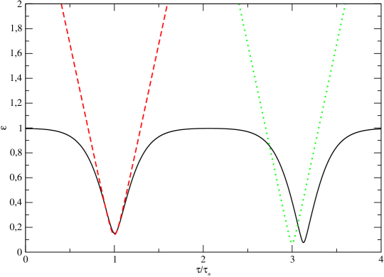
Figure 4: The numerically obtained dependency of $\epsilon$ on time shown as the solid line and the analytic expression given by eq. (46), where the dashed line corresponds to $\kappa=-$, while the dotted line corresponds to $\kappa=+$. The initial values of $i$, $e$ and $\omega$ are the same as the ones used in Figs 2 and 3.

IV The evolution of the dynamical system on a time scale much larger than $t_{*}$ and the role of Einstein precession

As we have mentioned above, the parameters describing our approximate solution slowly evolve with time when a large number of cycles are considered. This effect is determined both by unaccounted next-order corrections to our asymptotic solution, which is strictly valid only in the limit $e_{0},i_{0}\rightarrow 0$ and by additional effects causing the evolution of the orbital elements. Among the latter the most important role appears to be played by the Einstein apsidal precession, which is described by eq. (17), which should be added to the expression (14). We consider this role in this Section assuming that the parameter $\beta_{E}$ in eq. (17) is small. We also briefly discuss the role played by the next-order corrections in the purely Newtonian problem, limiting ourselves to numerical means in this Paper. We also set $\pi=\pi/2$ throughout this Section, assuming, for simplicity, that the perturbing potential is fully determined by the $|m|=2$ terms.

Since the rate of GW emission strongly depends on the values of $\epsilon_{min}^{\kappa}$, we need to know how the quantities entering eq. (43) evolve. There are some simple arguments based on the conservation of the full Hamiltonian (21), which allow us to assume that $e_{0}$ evolve slower than $\omega_{0}$ (or $\psi_{0}$) and $i_{0}$. Therefore, in this Section, we consider only the evolution of latter quantities.

It is evident from eq. (17) that the Einstein precession is most important during the evolution in the region of sharp jumps, when $\epsilon$ is close to its maximum values during a particular cycle. This suggests the following approximation scheme, which allows us to reduce the influence of the Einstein term to a simple map. That is, we assume that it operates only in the transition layers, while in the regions where $i$ is close to $0$ or $\pi$ its influence is negligible, and we can use our Newtonian asymptotic solution obtained above. However, the parameters $i_{0}$ and $\omega_{0}$ change their values as the system evolves through sharp jumps. The parameters are accordingly changed to new values $i_{1}$ and $\omega_{1}$ when the system evolves from the state with $i\sim 0$ to $i\sim\pi$ ($\kappa=-1$) and after the change of inclination from $\sim\pi$ to $\sim 0$ we have another change in the parameters $i_{1},\omega_{1}\rightarrow i_{2},\omega_{2}$. The values $i_{2},\omega_{2}$ are then considered as initial values of these parameters for the next cycle.

IV.1 The evolution of the angles $\omega$ and $\varpi$ in the region of sharp jumps which takes into account the Einstein precession

As has already been pointed out above when the system evolves in the region of sharp jumps $\sin(2\varpi)$ and $\cos(2\Omega)$ are small. This property remains to be valid when $\beta_{E}$ is small enough. It then follows that equations (41) still remain approximately valid even when $\beta_{E}$ is non-zero and we can use their solutions (46) to describe the evolution of $e$ and $i$. In order to find the evolution of $\omega$ and $\varpi$ we define $\Delta_{1}=\cos(2\Omega)$ and $\Delta_{2}=\sin(2\varpi)$, assume that the absolute values of $\Delta_{1,2}$ are small, express $\varpi$ and $\omega$ in eq. (14) and eq. (15) in terms of $\Delta_{1}$ and $\Delta_{2}$ taking into account that $2\omega\approx\kappa{\pi\over 2}-\kappa\Delta_{1}+2\pi k$, set $e=1$ and $\epsilon=0$ in the brackets on r.h.s. of eqns (14) and (15) and add eq. (17) to eq. (14). In this way we obtain

$${d\Delta_{1}\over d\tau}={20\over\epsilon}\Delta_{2},\quad{d\Delta_{2}\over d\tau}={20\kappa\cos i\over\epsilon}\Delta_{2}+{2\beta_{E}\over\epsilon^{2}}.$$ (47)

We substitute eq. (46) in eq. (47) and introduce a new time variable, $T$, according to the rule $T={20\over\epsilon_{*}}(\tau-\tau_{\kappa})$, where $\epsilon_{*}$ is any of $\epsilon_{min}^{\kappa}$. We have

$${d\Delta_{1}\over dT}={\Delta_{2}\over\sqrt{1+T^{2}}},\quad{d\Delta_{2}\over dT}={\Delta_{2}\over(1+T^{2})}+{\beta_{*}\over(1+T^{2})},$$ (48)

where we take into account that $\epsilon=\epsilon_{*}\sqrt{1+T^{2}}$ in the transition layers and $\beta_{*}={\beta_{E}\over 10\epsilon_{*}}$. A solution to eq. (48) should agree with eq. (38), which tells us that $|\Delta_{2}|\propto|T|$ in the limit $|T|\rightarrow\infty$. Such a solution to eq. (48) has the form

$$\Delta_{1}=(C+\beta_{*})T+\beta_{*}\sqrt{(1+T^{2})},\quad\Delta_{2}=(C+\beta_{*})\sqrt{(1+T^{2})}+\beta_{*}T.$$ (49)

The constant $C$ should be matched to the expressions (36-38) taken in the limit $e\rightarrow 1$ and $\epsilon\rightarrow 0$, where we should use $i_{0}$ and $\omega_{0}$ when $\kappa=-1$ and $i_{1}$ and $\omega_{1}$ when $\kappa=1$, as explained above. It is evident from eq. (49) that

$$\Delta_{1}(T\rightarrow-\infty)=CT,\quad\Delta_{1}(T\rightarrow\infty)=(C+2\beta_{*})T.$$ (50)

Thus, leaving aside the short time evolution of the state variables in the region of sharp jumps, one can see that the effect of Einstein precession leads to redefinition of the constant $C$, which, in its turn, leads to redefinitions of the angles $\omega_{0}$ and $i_{0}$ as has been pointed out above. That allows us to describe the influence of Einstein precession in terms of an iterative map linking ’old’ and ’new’ values of $\omega_{0}$ and $i_{0}$. This map is analyzed in Appendix B. As shown there this map has the property that one of $\epsilon^{\kappa}$ always grows, while another one always decreases with the number of its iterations $n$.

IV.2 An estimate of a minimal value of $\epsilon$ in case when $\beta_{E}$ is relatively large

From equations (84-88) of Appendix B it follows that $i_{0}$ as well as either $\epsilon^{-}$ or $\epsilon^{+}$ tend to infinity with $n$. This clearly violates our basic assumptions, and, therefore, our treatment is valid only for a finite value of cycles. As a criterion of violation of our assumption we suppose that they are broken when $\Delta_{1}=\cos(2\omega)$ is order of one when $i=\pi/2$. Remembering that the latter condition corresponds to $T=0$ we have from equation (49) $\Delta_{1}(i=\pi/2)=\beta_{*}={\beta_{E}\over 10\epsilon_{*}}$, and, from the condition $\Delta_{1}<\beta_{*}$ we obtain

$$\epsilon_{*}>\epsilon_{min}={\beta_{E}\over 10},$$ (51)

and, using either eqns (87) and (88) we conclude that our map is expected to be valid when $n<n_{max}$, where $n_{max}\approx\Lambda({5{i_{0}(0)}^{2}|\sin(2\psi_{0}(0))|\over\beta_{E}})$ and $\Lambda=\log({10i_{0}(0)|\sin\psi_{0}\over e_{0}^{1/5}\beta_{E}})$ when $\sin(2\psi_{0}(0))>0$ and $\Lambda=\log({10i_{0}(0)|\cos\psi_{0}\over e_{0}^{1/5}\beta_{E}})$ in the opposite case.

The inequality (51) also follows from another quite general argument. Namely, we can estimate a minimal possible value of $\epsilon$, which can in principle be reached when $\beta_{E}$ is non-zero using the fact that Hamiltonian is the integral of motion. For that, we note that from eq. (18) it follows that the contribution to the Hamiltonian due to the presence of Einstein precession is always negative, and, on the other hand, it follows from eq. (9) that the corresponding terms due to the tidal terms can be positive. It is possible to show that when $e_{0}$ and $i_{0}$ are small, but, on the other hand we consider the state of the system with $e\sim 1$ and $i\sim\pi/2$, their separate absolute values are much larger than a value of Hamiltonian, so they should compensate each other. Setting $e=1$ and $i=\pi/2$ in eq. (9), and assuming that the value of the total Hamiltonian is equal to zero we obtain

$$5\cos(2\omega)(\cos(2\varpi)+1)-{\beta_{E}\over\epsilon}\approx 0.$$ (52)

The first term in eq. (52) cannot be larger than $10$, which corresponds to $\cos(2\omega)=\cos(2\varpi)=1$. Setting it equal to $10$ we obtain the expression for $\epsilon_{min}$.

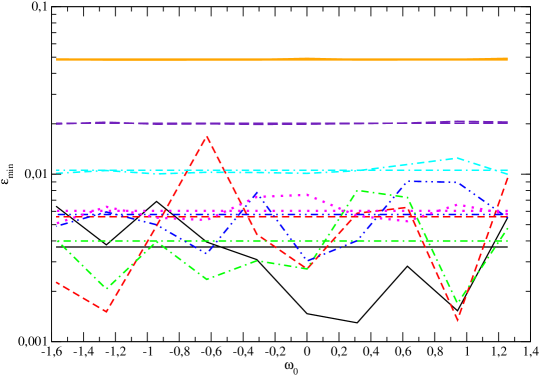
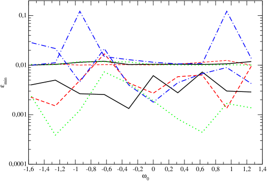
Figure 5: Top panel. The minimal values of $\epsilon_{min}$ found numerically over the calculation time corresponding to $10^{2}$ cycles ($\sim 400\tau_{*}$) as functions of the initial nodal angle $\omega_{0}$. $e_{0}=i_{0}=0.1$ for all runs. Different curves correspond to different values of $\beta_{E}$ with the horizontal lines of the same style showing the averaged over $\omega_{0}$ values of $\epsilon_{min}$. The solid curves and horizontal lines represent $\beta_{E}=0$ (black) and the largest considered $\beta_{E}=0.5$ (orange), with the larger values corresponding to $\beta_{E}=0.5$. Note that in the latter case $\epsilon_{min}$ practically coincides with its average value. The short dashed, dot dashed, double dot dashed, dotted, dot double dashed, long dashed curves are for $\beta_{E}=10^{-3}$ (red), $0.1$ (green), $0.025$ (blue), $0.05$ (magenta), $0.1$ (cyan) and $0.2$ (violet), respectively. Bottom panel. The same as top panel, but different curves correspond to different values of $i_{0}$. $e_{0}=0.1$ for all curves. The curves of the same style with larger (smaller) values correspond to $\beta_{E}=0.1$ ($\beta_{E}=0.001$). Solid black, dashed red, dotted green and dot dashed blue curves are for $i_{0}=0.05$, $0.1$, $0.2$ and $0.5$, respectively.

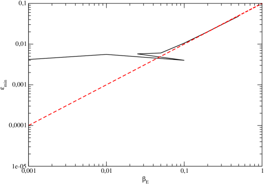
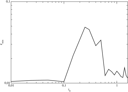
Figure 6: Top panel. The value of $\epsilon_{min}$ averaged over the initial nodal angle $\omega_{0}$ as a function of $\beta_{E}$ is shown as a solid line. $e_{0}=i_{0}=0.1$ for the shown case. The dashed line represents the theoretical value (51). Bottom panel. The same quantity calculated numerically as a function of $i_{0}$. We use $e_{0}=\beta_{E}=0.1$ for all calculations.

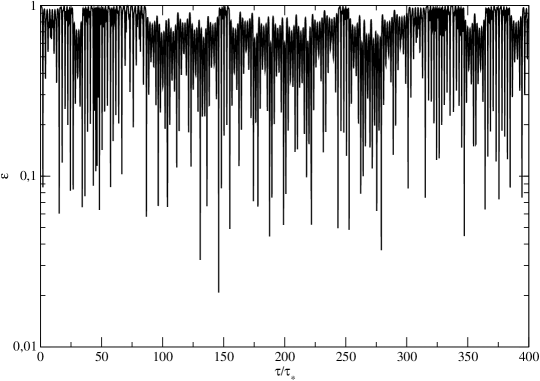
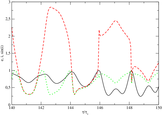
Figure 7: Top panel. The value of $\epsilon_{min}$ as a function of time numerically obtained for the calculation with $e_{0}=\beta_{E}=0.1$, $i_{0}=\pi/4$ and $\omega_{0}=\pi/3$. We show the whole time period $t<t_{end}$. Bottom panel. $e$ (solid line), $i$ (dashed line) and $\sin(i)$ (dotted line) as functions of time shown in the time interval $140<\tau/\tau_{*}<150$.

IV.2.1 A minimal value of $\epsilon_{*}$ obtained from a numerical analysis of our system

In order to check the analytic approach discussed above we perform a set of numerical runs with different initial parameters. The initial eccentricity $e_{0}$ is set to be equal to $0.1$ for all runs, but we consider several initial inclinations $i_{0}$ in the range $0.05-1.6$, the parameter $\beta_{E}$ in the range $0-0.5$ and ten values of the initial nodal angle $\omega_{0}$ uniformly distributed in the interval $(-\pi/2..\pi/2)$ . The end time of the computation, $t_{end}$, is chosen in such a way that approximately $100$ evolutionary cycles are executed in a particular computational run. From the results discussed above it follows that every cycle has a period $\approx 4\tau_{*}$, where $\tau_{*}$ is given by eq. (30), and, therefore We end up the computations when $t=t_{end}=400\tau_{*}$. From equations (11) and (30) we see that $t_{end}$ in the physical units can be represented as

$$t_{end}\approx 160\log({8\over e_{0}^{2}}){n_{0}\over\Omega^{2}}\approx 10^{3}{n_{0}\over\Omega^{2}},$$ (53)

where we set $e_{0}=0.1$ to obtain the last equality. We obtain minimal values of $\epsilon$ for each run and compare them with our analytic estimates.

The results of the comparison are shown in Figs. 5 and 6. In top panel of Fig. 5 we plot the so obtained numerical values of $\epsilon_{min}$ versus $\omega_{0}$ for our ’standard choice’ of the initial eccentricity and inclination $e_{0}=i_{0}=0.1$. Curves of different style and color correspond to different values of $\beta_{E}$ and we also show the averaged over $\omega_{0}$ values of $\epsilon_{min}$ as horizontal lines of the same style and color, see the figure caption for a description of particular lines. As seen from this plot when $\beta_{E}>\sim 0.05$ the values of $\epsilon_{min}$ quite weakly depend on $\omega_{0}$. At smaller values of $\beta_{E}$ the curves are less uniform, but particular values of $\epsilon_{min}$ deviate from the averaged one by factor of a few even in this case. In bottom panel of the same figure we plot $\epsilon_{min}$ corresponding to different initial inclinations as functions of $\omega_{0}$ for $e_{0}=0.1$ and two representative values of $\beta_{E}=10^{-3}$ and $0.1$. As seen from this plot, in general, the curves with different values of $i_{0}$ do not deviate much from each other when $i_{0}$ is sufficiently small.

In Fig. 6 we show the averaged value of $\epsilon_{min}$ as a function of $\beta_{E}$ for $e_{0}=i_{0}=0.1$ in top panel and the same quantity as function of $i_{0}$ for $e_{0}=\beta_{E}=0.1$ in bottom panel. In top panel the solid curve represents the numerical results, while the dashed line shows our expression for $\epsilon_{min}$ given in eq. (51). As seen from this Fig. when $\beta_{E}>0.05$ we have an excellent agreement between the numerical results and our analytic expression. In this opposite case $\beta_{E}<0.05$ $\epsilon_{min}$ is almost constant, while when $\beta_{E}\sim 0.05$ the numerical curve shows a complicated behaviour. In general, the numerical curve agrees with our previous analysis. When $\beta_{E}$ is significantly large the effect of Einstein precession gives the main contribution to the evolution of the approximate constants of motion characterizing our approximate asymptotic solution discussed in the previous Section, and, accordingly, to the evolution of $\epsilon_{min}$ from one cycle to another. In the opposite case this role is played by non-linear corrections to the asymptotic solution, which do not depend on $\beta_{E}$. We have, accordingly, an almost constant dependency of $\epsilon_{min}$ on $\beta_{E}$ in the latter case. In what follows we are going to use a very simple approximation of this dependency. Namely, we are going to assume that

$$\epsilon_{min}(\beta_{E}>0.05)={\beta_{E}\over 10},\quad\epsilon_{min}(\beta_{E}<0.05)=5\cdot 10^{-3}.$$ (54)

Bottom panel of this Fig. shows that the dependency of the averaged $\epsilon_{min}$ on $i_{0}$ is non-monotonic. It agrees with our theoretical value $\epsilon_{min}(\beta_{E}=0.1)=0.01$ only when $i_{0}<\sim 0.1$. When $i_{0}$ gets larger $\epsilon_{min}$ increases, then it decreases back to values $\sim 0.011-0.15$.

Interestingly, the average value of $\epsilon_{min}$ is quite small even when $i_{0}\approx\pi/2$. This is important for our purposes, since it greatly extend an available phase space of orbits with small eccentricities, which can experience an efficient circularization due to GW emission. The case of large initial inclinations cannot be treated, however, in framework of the simple theory developed above.

In order to illustrate the behaviour of our system in case of a large $i_{0}$ we show time the time dependency of $\epsilon$ for the whole time interval $0<t<t_{end}$ in Fig. 7, top panel for $i_{0}=\pi/4$ and $\beta_{E}=0.1$. As seen from this Fig. the values of $\epsilon$ can be as small as $\sim 2\cdot 10^{-2}$ in this particular case. A smaller time interval containing the moment of time $\tau\approx 144\tau_{*}$ corresponding to the smallest value of $\epsilon$ is shown in bottom panel of the same Fig. We show the dependencies of $e$, $i$ and $\sin(i)$. The dynamics of the variables at the time $<\sim 146$ is in qualitative agreement with our previous results. The minimal values of $i$ are about $0.3$ and the minimal values of eccentricity are about $0.5-0.6$, the maximal values of eccentricity are reached at times, which are close to the times corresponding to $\sin(i)=1$ ($i=\pi/2$) and the cycle period is close to $4\tau_{*}$. Therefore, it is possible to have a transient dynamics with relatively small minimal values of inclinations and intermediate values of eccentricity even when the initial value of inclination is large.

V Final stages of SBBH evolution and emission of GWs

If at final stages of evolution two components in SBBH are close enough emission of GWs could play important role in the evolution of SBBH at these stages. In this Section we give an order of magnitude estimations of SBBH parameters when such situation takes place.

For this purpose, it is enough to leave in the perturbing potential (see equation (1)) the terms with $|m|=2$ only.

In what follows we use empirical relationships between the effective radius of NSC, the mass of the central primary black hole, $M_{p}$, and the radius of influence of the primary, $r_{infl}$, proposed in [38]. For simplicity, we consider only the early-type galaxies; also see [38]. As follows from Fig. 8 of this Paper the effective radius of such galaxies is of the same order as $r_{infl}$. For this reason and for reason of simplicity, we assume that they these radii are close to each other. Then after simple manipulations with some parameters presented in Table 1 of this Paper we can see that

$$r_{infl}\approx 23\alpha_{r}M_{8}^{0.35}pc,$$ (55)

where $M_{8}=M_{p}/(10^{8}M_{\odot})$ and the parameter $\alpha_{r}$ is expected to be of the order of unity. Then, assuming that inside $r_{infl}$ the stellar density, $\rho_{st}(r)$, follows the well known profile $\rho_{st}(r)\propto r^{-3/2}$ [39], we have

$$M_{st}(r<r_{infl})\approx M_{p}({r\over r_{infl}})^{3/2},$$ (56)

where $M_{st}(r)$ is stellar mass in NSC within a given radius $r$. If (as we have already mentioned in the Introduction) the mass ratio of the black holes, $q=M_{s}/M_{p}$, is small, dynamical friction is expected to be efficient until the SBBH semi-major axis, $a$, is larger than a scale where the stellar mass enclosed within the orbit is of the order of the mass of the secondary black hole, $M_{s}$. Introducing a new parameter $\alpha_{s}$ such as $M_{st}(r=a)=\alpha_{s}M_{s}$, from eq. (56) we can see that the latter equation is satisfied when

$$a\approx 4.6\cdot 10^{-2}\alpha_{s}^{2/3}q_{-2}^{2/3}r_{infl}=1.1\alpha_{r}\alpha_{s}^{2/3}q_{-2}^{2/3}M_{8}^{0.35}pc,$$ (57)

where $q_{-2}=10^{2}q$.

We assume that when the semi-major axis is approximately equal to the expression (57) the stars inside the orbit are quickly dispersed by the secondary and there is no significant inflow of stars to the radii $r\sim a$ from the outer part of the system. Consequently, the evolution of $a$ is supposed to stop when its value is approximately equal to (57). The orbital motion is then mainly determined by the Newtonian gravitational field of the primary at relatively short timescales, and at larger timescales the secular evolution of the orbital elements is assumed to be determined by the tidal field of non-spherical NSC and the Einstein precession of the apsidal line as discussed above as well as the effect of GW emission in the case of highly eccentric orbits.

Typical values of the mean motion $n_{0}=\sqrt{GM_{p}\over a^{3}}$ and the orbital period $P_{orb}=2\pi/n_{0}$ can be directly estimated from eq. (57) as

$$n_{0}=1.8\cdot 10^{-3}\alpha_{r}^{-3/2}\alpha_{s}^{-1}q_{-2}^{-1}M_{8}^{-0.025}yr^{-1},\quad P_{orb}=3.4\cdot 10^{3}\alpha_{r}^{3/2}\alpha_{s}q_{-2}M_{8}^{0.025}yr.$$ (58)

In order to estimate typical values of the timescales $t_{*}$ and $t_{end}$ characterizing the secular evolution due to the tidal effects and given by eqns (11) and (53), respectively, we need to parametrize the frequency $\Omega$ determining the strength of the tidal potential (2) in a convenient way. We represent it in the form

$$\Omega=\sqrt{\mu GM_{p}\over r_{infl}^{3}},$$ (59)

where the dimensionless coefficient $\mu$ determines a degree of non-sphericity of NSC. It is small when NSC is only slightly non-spherical. We substitute eq. (55) in eq. (59) and eq. (59) in eqns (11) and (53) and, taking into account eq. (58) we obtain

$$t_{*}\approx 1.9\cdot 10^{7}\alpha_{r}^{3/2}\alpha_{s}\mu^{-1}q_{-2}^{-1}M_{8}^{0.025}yr,\quad t_{end}\approx 250t_{*}=4.9\cdot 10^{9}\alpha_{r}^{3/2}\alpha_{s}\mu^{-1}q_{-2}^{-1}M_{8}^{0.025}yr.$$ (60)

It is convenient to represent relativistic parameter $\beta_{E}$, defined in eq. (17), in terms of dimensionless variable $u=GMc^{-2}a^{-1}$ which is proportional to the ratio of the gravitational radius of primary black hole to the semi-major axis of secondary black hole orbit. Then taking to account eq. (57) we obtain

$$u={GM\over c^{2}a}=4.4\cdot 10^{-6}\alpha_{r}^{-1}\alpha_{s}^{-3/2}q_{-2}^{-2/3}M_{8}^{0.65}.$$ (61)

Using this definition we represent the parameter $\beta_{E}$ as $\beta_{E}=12u\Omega^{2}n_{0}^{-2}$, and, using eqns (57), (59) and (61) we obtain

$$\beta_{E}=0.54\alpha_{r}^{-1}\alpha_{s}^{4/3}\mu^{-1}q_{-2}^{-8/3}M_{8}^{0.65}.$$ (62)

According to eq. (62) for the considered typical parameters of the binary and NSC the effect associated with the Einstein precession is relatively large, and, therefore, this effect should be definitely taken into account.

Let us consider now the possibility of the orbital circularization due to emission of gravitational waves by SBBH with $\epsilon\ll 1$. We can use the result of [49] for the evolution of semi-major axis for orbits with a small mass ratio $q$ and eccentricity close to one:

$$({\dot{a}\over a})_{GW}\approx-{170\over 3}{qu^{5/2}n_{0}\over\epsilon^{7}}.$$ (63)

As a criterion of an efficient orbital circularization we use the condition that the associated characteristic evolution time $t_{GW}=|({a\over\dot{a}})_{GW}|^{-1}$ is smaller than the orbital period $P_{orb}$. This results in the condition

$$q_{-2}>{3\over 3.4\pi}\alpha_{r}^{5/2}\alpha_{s}^{5/3}\epsilon^{7}u^{-5/2}.$$ (64)

Both dimensionless factors $u^{5/2}$ and $\epsilon^{7}$ are quite small. In order to single out the small numerical factor in $\epsilon^{7}$ we normalize it to the smallest expected value $5\cdot 10^{-3}$ (see eq. (54) using $\tilde{\epsilon}=\epsilon/(5\cdot 10^{-3})$. Substituting $\epsilon^{7}=7.8\cdot 10^{-17}{\tilde{\epsilon}}^{7}$ and eq. (61) in eq. (64) we obtain

$$\tilde{\epsilon}<\epsilon_{max}=2.9\alpha_{r}^{-5/14}\alpha_{s}^{-5/21}q_{-2}^{-0.095}M_{8}^{0.23}.$$ (65)

The inequality (65) can be satisfied when $\tilde{\epsilon}>1$, hence, inequalities (65) and (51) are compatible, and, accordingly, we can use $\epsilon\approx\beta_{E}/10$ , and obtain from eq. (62)

$$\tilde{\epsilon}\approx 54\alpha_{r}^{-1}\alpha_{s}^{4/3}(0.1/\mu)q_{-2}^{-8/3}M_{8}^{0.65}.$$ (66)

Using this estimate we can reformulate eq. (65) as

$$q_{-2}>\leavevmode\nobreak\ 3.1\alpha_{r}^{-0.25}\alpha_{s}^{0.61}({0.1\over\mu})^{0.38}M_{8}^{0.16}.$$ (67)

Note a rather weak dependence on the quantities on r.h.s.

On the other hand, eq.(54) tells that we assume , for our estimates, that $\tilde{\epsilon}$ cannot be smaller than one. Setting $\tilde{\epsilon}=1$ in l.h.s of eq. (66) we have

$$M_{8}>\sim 2\cdot 10^{-3}\alpha_{r}^{1.5}\alpha_{s}^{-2}{({\mu\over 0.1})}^{1.5}q_{-2}^{4}.$$ (68)

Thus, for a given mass ratio our approach is valid only for sufficiently massive primary black holes.

Using the Newtonian relationship between the orbital periastron $r_{p}$ and the semi-major axis, $r_{p}=(1-e)a$, we can easily estimate from eq. (61) a typical value of periastron corresponding to SBBHs, which evolve due to the emission of GWs.

$$r_{p}\approx 11.2\alpha_{r}\alpha_{s}^{2/3}q_{-2}^{-2/3}M_{8}^{-0.65}{\tilde{\epsilon}}^{2}{GM_{p}\over c^{2}}=4.1\alpha_{r}^{5/4}\alpha_{s}^{1/3}({\mu\over 0.1})^{1/4}M_{8}^{-0.81}{\tilde{\epsilon}}^{2}{GM_{p}\over c^{2}},$$ (69)

where we use eq. (66) to express the mass ratio in terms of other parameters of the problem. Thus, when all quantities in the last equality on r.h.s. have their nominal values, $r_{p}$ turns out to be close the radius of the marginally bound orbit for a Schwarzschild primary black hole $r_{mb}={4GM\over c^{2}}$, which is the minimal possible periastron for parabolic orbits. Those orbits, which have periastra formally smaller than $r_{mb}$ directly plunge into black hole. Therefore, our model implies that, for certain system’s parameters, there could be processes of direct black holes collisions from parabolic orbits, or, in case when $r_{p}$ is larger than but comparable to $r_{mb}$, there could be a substantial eccentricity during the whole merger process.

In order to illustrate this property of our model let us formally assume that effects of General Relativity are small, and the relation between eccentricity and semi-major axis during the orbital evolution caused by GW emission is given by equation (5.11) of [49] valid in the limit of weak gravity,

$$a(e)=c_{0}f(e),\quad f(e)={e^{12/19}\over(1-e^{2})}(1+{121\over 304}e^{2})^{870/2299},$$ (70)

To express $c_{0}$ in terms of $r_{p}$ given by eq. (69)we consider the limit $e\rightarrow 1$ in eq. (70) and obtain that

$$c_{0}\approx{2r_{p}\over(1+{121\over 304})^{870/2299}}\approx 19.7\alpha_{r}\alpha_{s}^{2/3}q_{-2}^{-2/3}M_{8}^{-0.65}{\tilde{\epsilon}}^{2}{GM_{p}\over c^{2}}=7.2\alpha_{r}^{5/4}\alpha_{s}^{1/3}({\mu\over 0.1})^{1/4}M_{8}^{-0.81}{\tilde{\epsilon}}^{2}{GM_{p}\over c^{2}}.$$ (71)

Using eq. (70) we can also calculate a typical GW frequency, $\nu_{GW}={2\over P_{orb}}$, where the factor two takes into account the quadrupole character of GW emission. We have from eq. (70)

$$\nu_{GW}={1\over\pi}\sqrt{GM_{p}\over c_{0}^{3}f(e)^{3}}=3.3\cdot 10^{-5}\alpha_{r}^{-15/8}\alpha_{s}^{-1/2}{({\mu\over 0.1})}^{-3/8}M_{8}^{0.21}{\tilde{\epsilon}}^{-3}{f(e)}^{3/2}Hz.$$ (72)

We plot several curves showing the dependencies of $e$ on $a$ and $e$ on $\nu_{GW}$ for several values of $\tilde{\epsilon}$ setting any other parameters in the last expression on r.h.s of eq. (71) to their nominal values in Fig. 8. The range of shown semi-major axes is bounded from below by the condition $r_{p}>r_{mb}={4GM_{p}\over c^{2}}$. Note that the condition $r_{c}=r_{mb}$ describes correctly the boundary between orbits having periastra and the plunging orbits only when eccentricity is close to unity. We still use it, nevertheless, for any eccentricity, since in any case our oversimplified approach can be used for qualitative purposes only.

One can see from this Fig. that the formation of substantial eccentricities for values of $a$ comparable with gravitational radius, or even the direct black holes collision are possible when $\tilde{\epsilon}$ is close enough to unity. But, as we have mentioned above this conclusion has only qualitative character. For quantitative conclusions a calculation based on full General Relativity is needed, see e.g. [50], [51], [52] and references therein. Also, in all shown cases eccentricities are of the order of $\sim 0.1-0.3$ in the range of typical GW frequencies available for LISA $\nu_{GW}>\leavevmode\nobreak\ 10^{-5}Hz$, see e.g. [8]. We can rewrite eq. (66) as

$$q_{-2}\approx 4.5\alpha_{r}^{-3/8}\alpha_{s}^{1/2}{({0.1\over\mu})}^{3\over 8}M_{8}^{0.24}{\tilde{\epsilon}}^{-3/8}.$$ (73)

Equation (73) tells that the condition $\tilde{\epsilon}\approx 1$ correspond to a particular relatively large mass ratio when all other parameters of the problem are fixed, see also eqns (67) and (68).

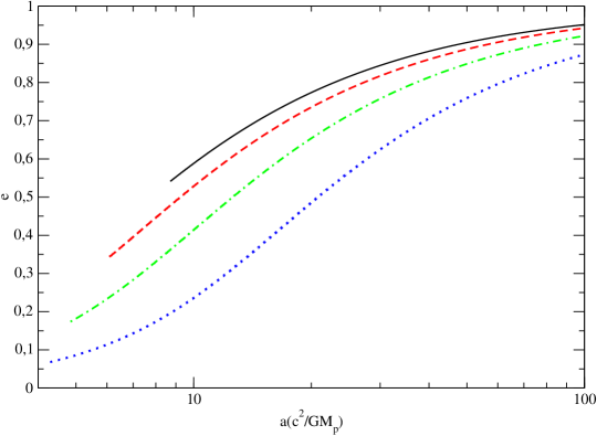
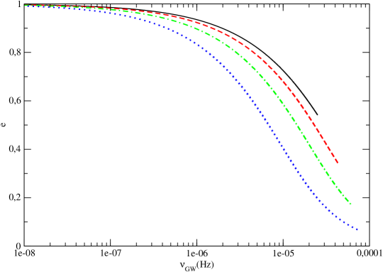
Figure 8: Top panel. We show the dependency (70) calculated for $c_{0}=7.2{\tilde{\epsilon}}^{2}{GM_{p}\over c^{2}}$ corresponding to the nominal values of all quantities in the second expression on r.h.s. of eq. (71) on the plane $(({c^{2}\over GM_{p}})a,e)$. The solid, dashed, dot dashed and dotted curves correspond to $\tilde{\epsilon}=1.1$, $1.2$, $1.4$ and $1.8$, respectively. Bottom panel. The dependency of eccentricity on the typical frequency of GW emission calculated according to eq. (72). Curve of the same type as in left panel correspond to the same value of $\tilde{\epsilon}$.

VI Conclusions and Discussion

In this Paper we consider a secular evolution of a gravitationally bound binary black hole with unequal mass ratio in a center of non-spherical Nuclear Star Cluster (NSC) around the component with a larger mass (primary). The semi-major axis of the binary is supposed to correspond to the radius, where an initial mass of the cluster is equal to the mass of the smaller component (secondary), which is smaller than the radius of influence of the primary. At this radius the evolution of the semi-major axis due to dynamical friction is supposed to be stalled and the stellar mass in the vicinity of the orbit is supposed to be quickly dispersed by the perturbing action of the secondary. Assuming that these model assumptions are valid we consider the secular orbital evolution due to tidal forces arising from the non-spherical gravitational field of NSC, which are treated in the usual quadrupole approximation. We note that by rotation of a coordinate system we can always bring the tidal potential to the form, where only $m=0$ and $m=2$ terms in its decomposition over spherical harmonics remain. The $m=0$ term is responsible for the usual ZLK secular dynamics, while the secular dynamics due to $m=2$ terms has not, to the best of our knowledge, been explored so far in the context of SBBH orbital evolution. Note, however, that in the case of stellar mass binaries evolving in an external field of a star cluster a similar problem was considered by [34], where some numerical calculations and a qualitative analysis were made with the similar conclusions on the possibility of reaching very large values of eccentricity at sufficiently large times. Also, the secular dynamics of stars in a triaxial stellar cluster around a supermassive black hole was discussed in [53], where the possibility of reaching of very large eccentricities was investigated by analytic and numerical means.

Since in the course of the evolution determined by $m=2$ terms all three components of angular momentum are not conserved, it can potentially lead to the formation of highly eccentric orbits from the orbits with a small or moderate eccentricity, which can, in its turn, promote to an efficient evolution of semi-major axis due to GW emission. Therefore, we consider this evolution in some detail using analytic and numerical means.

Since the set of equations describing the secular dynamics under the influence of the $m=2$ terms cannot be analytically integrated even when the simplest case when only the influence of these terms is taken into account we have to consider some simplifying assumption. The main technical assumption made in this work is that there is a moment of time $t=t_{0}$ in the course of the evolution of our system when eccentricity $e_{0}$ and inclination to the symmetry plane $i_{0}$ are small. It then follows that it is possible to construct a singular solution, which is similar to solutions describing ideal shocks in hydrodynamics in that sense that it also contains discontinuities. This solution is formally valid in the limit $i_{0}\rightarrow 0$. It is shown that this solution describes periodic cycles of the evolution. Within every cycle there are two equal time periods corresponding to inclination $i$ being either infinitesimally close to $0$, or to $\pi$. These periods are separated by two moments of time corresponding to the transitions of inclination from $0$ to $\pi$ and back. During these transitions the eccentricity $e$ formally reaches unity. We find time period of such a solution assuming that $e_{0}$ is small and show that it is fully characterized by $e_{0}$ and a value of the nodal angle at the moment $t_{0}$, $\omega_{0}$.

When a small, but finite $i_{0}$ is considered the transitions of $i$ from $0$ to $\pi$ and back are smeared to a small, but finite periods of time. We call these periods as ”sharp jumps” Also, the eccentricity $e$ reaches a large, but a finite value, which happens at the moment of time close to the moment of time when $i=\pi/2$. We calculate the minimal values of $\epsilon=\sqrt{1-e^{2}}$, $\epsilon^{\mp}_{min}$, where $(-)$ corresponds to the transition of $i$ from $0$ to $\pi$ and $(+)$ corresponds to the opposite transition, and show, that they are proportional to trigonometric functions of $\omega_{0}$ and inversely proportional to $i_{0}$. Thus, the analytic theory shows that eccentricity can be made as large as necessary provided that either $i_{0}$ is chosen to be sufficiently small or $\omega_{0}$ is equal to some special values.

When next order corrections to our asymptotic solution or other factors causing a secular evolution of the orbital elements are considered $i_{0}$, $e_{0}$ and $\omega_{0}$ are slowly changing from one cycle to another. This also results in a slow evolution of $\epsilon^{\mp}_{min}$, which can, accordingly, reach other values than the ones corresponding to the initial cycle when a large, in comparison with the period of the cycle time is considered. In this Paper we consider analytically the most important relativistic factor - the Einstein precession of the apsidal line leaving an analytic treatment of the next order corrections and other factors for a possible future work. It is shown that the role of Einstein precession is determined by the parameter $\beta_{E}$ defined as the ratio of characteristic time of the Einstein precession to that of the secular evolution due to the tidal effects. Based on the law of conservation of Hamiltonian during the secular evolution we argue that a change of $e_{0}$ on the long timescale is expected to be smaller than those of $\omega_{0}$ and $i_{0}$ and show that the minimal possible value of $\epsilon^{\mp}_{min}$ should be $\beta_{E}/10$. It is then shown that the effect of a non zero, but sufficiently small $\beta_{E}$ can be described as a map between $i_{0}$ and $\omega_{0}$ corresponding to subsequent cycles. This map has the property that either $\epsilon^{-}$ always grows and $\epsilon^{+}$ always decreases or vice versa in the course of the evolution.

The analytic results are supplemented by the results based on numerical solution of the dynamical evolution. First, we show for a purely Newtonian problem, that when the contribution of $m=0$ term to the full Hamiltonian isn’t too large the evolution is qualitatively the same as described above. Next, we consider a large number of cycles taking, for definiteness, approximately $100$ cycles and evaluate numerically the minimal $\epsilon$ over the whole computational time, $\epsilon_{min}$. We use $e_{0}$ for all runs and different values of $\omega_{0}$, $i_{0}$ and $\beta_{E}$. It is shown numerically that the averaged over $\omega_{0}$ value of $\epsilon_{min}$ is close to $\beta_{E}/10$ when $\beta_{E}>0.05$, for smaller value of $\beta_{E}$ it is close to constant. This result in full agreement with our theoretical findings, the constant value of $\epsilon_{min}$ at small values of $\beta_{E}$ is interpreted as being determined by the evolution of $\omega_{0}$ and $i_{0}$ due to the next order corrections.

We use these results to estimate a possibility of an efficient capture of the secondary having initially an orbit with a small eccentricity $\sim 0.1$ onto an orbit with semi-major axis strongly decreasing due to GW emission in a time corresponding to $100$ cycles of the secular evolution. As a criterion of such strong evolution we choose the condition that the semi-major axis should decrease by order of itself per one orbital period. We use an empirical relation between the size of NSC and the primary mass suggested from observations for early type galaxies, the assumption that the radius of influence is the same by order of magnitude as the size and the standard Young profile for the distribution of stellar density inside the sphere of influence. We estimate that for typical masses of the primary and total mass of NSC in the non-spherical component order of ten per cent the mass ratio should be larger than $0.04$ to fulfill our criterion of the efficient capture. The capture time is estimated to be smaller than several billion years corresponding to $100$ cycles of the secular evolution for the assumed typical value of the radius of influence $r_{infl}\sim 20pc$. When $r_{infl}$ is ten times smaller, the evolution time is expected to be $\sim 10^{8}yr$, see eq. (60). Thus, the considered mechanism provides an alternative for a solution of the final parsec problem.

Our estimates of the maximal $\epsilon$, and maximal mass ratio $q$ and the primary mass $M_{p}$ required for the the efficient circularization due to our effect are given by eqns (65), (67) and (68), respectively. It is interesting to note that they contain rather small powers of the parameters of the problem on r.h.s. This is due to the fact these estimates were obtained by consideration of relative importance of two competing effects. While in order to have a relatively fast secular orbital evolution due to the non-sphericity of NSC larger semi-major axes are preferable, in order to have a faster evolution due to GW emission we need to consider smaller $a$. As a consequence the role of these process is somewhat compensated in the resulting expressions.

Assuming that the distribution of the secondary orbits over $i_{0}$ is uniform a number of systems where our analytical theory is directly applicable is quite small, being proportional to $i_{0}^{2}$. However, our numerical results suggest the values of $\epsilon$ as small as the ones corresponding to small $i_{0}$ can be obtained for $i_{0}$ as large as $\pi/2$ when the sufficiently large evolution time is considered, see Fig. 6. A possible explanation of this result is that over a large time there are transient periods of the evolution with sufficiently small minimal values of inclination, where the theory described above is qualitatively valid. This is illustrated in Fig. 7. Note that similar results have also been obtained by [34], who considered a long term evolution of a stellar mass binary under the action of a similar, but different perturbing potential.

Contrary to the usual scenarios of a SMBBH orbital evolution due to dynamical hardening our mechanism leads to a prompt formation of a binary evolving due to GW emission with its orbital periastron comparable to gravitational radius of the larger component. For certain parameters of the problem, its eccentricity may remain to be appreciable all the way down to the merger, or even the direct black hole collision is possible during the stage of orbital evolution caused by GW emission. Therefore, binaries formed by this mechanism may be distinguished from the standard ones by a form of gravitational wave signal. In this connection it is also interesting to note that the standard model of the activity of OJ 287 implies the existence of a binary with similar parameters.

Going back to the Newtonian problem it is interesting to stress the differences of the effect considered above from the usual ZLK case. One striking difference is that in the case of ZLK the projection of angular momentum onto the axis perpendicular to the symmetry plane $\propto\cos(i)$ is conserved, and, therefore, the largest values of $e$ (the smallest values of $\epsilon$ over an evolutionary cycle correspond to $i\leq\sqrt{\sin^{-1}({2\over 5})}$, while in our case the largest values are reached when $i\sim\pi/2$. Another difference is that in the former case the additional integral of motion significantly constraints the smallest values of $\epsilon$, which can be obtained.

There are many possible ways of extension of the results reported in this work. One can consider the evolution of the primary due to dynamical friction down to the radius, where it is assumed to be stalled in stellar cluster with a broken spherical symmetry and inner cusp, see e.g. [21] for an appropriate investigation, but in the case of a spherical initial stellar distribution. Other perturbing factors, such as e.g. the influence of gravitational potential of the stars in the vicinity of the orbit (see e.g [33] and [55]) should be considered. The general perturbing potentials having both $m=0$ and $m=2$ terms should be studied as well as the influence of the neighboring stars. Also, the evolution of orbital elements due to GW emission should definitely be treated in a more accurate way, which can be based on the post-Newtonian expansion of equations of motion (e.g. [56], [57] and references therein) or using a relativistic approximation scheme based on a small mass ratio of the black holes (e.g. [50], [51], [52] and references therein). It is clear that the general consideration can only be done by numerical means. This is left for a future work.

Finally, we would like to note that our results can be potentially applied in other astrophysical settings. For example, one can consider a binary star or an exoplanetary system inside a massive non-spherical protostellar cloud. Tidal forces acting from the cloud may influence the secular dynamics of a considered system in a way similar to what is discussed above.

Appendix A The evolution of $\epsilon$ in case when $\phi\neq\pi/2$

For simplicity, we do not provide the same asymptotic analytic treatment for the general case, when $\phi\neq\pi/2$ and both sets of dynamical equations (10) and (12-13) contribute to the evolution of our system according to the rule (7). However, we have made a set of additional numerical calculations choosing the same ’standard’ initial values of the dynamical variables as in Figs 2 and 3, but varying $\phi$ from $0$ to $\pi/2$. The result of calculations of $\epsilon$ for these cases is shown in Fig. 9.

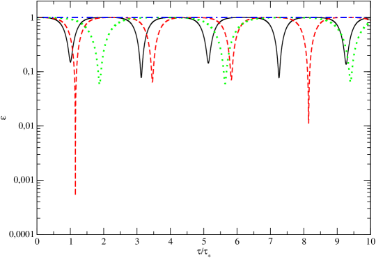
Figure 9: The numerically obtained dependencies of $\epsilon$ on time for different values of $\phi$. The initial values of $i$, $e$ and $\omega$ are the same as the ones used in Figs. 2 and 3. The solid, dashed, dotted and dot dashed curves correspond to $\phi=\pi/2$, $3\pi/8$, $\pi/4$ and $\pi/8$, respectively.

One can see from this Figure that the dependency of the values of minimal $\epsilon$ on $\phi$ is non-monotonic. Note a very small value of the minimal $\epsilon$ in case when $\phi=3\pi/8$. Even in the case when $\phi=\pi/4$ and, accordingly, the terms with $m=0$ and $m=2$ give the same contribution to the perturbing potential the values of minimal $\epsilon$ are close to, but smaller than in the case $\phi=\pi/2$, where only the $m=2$ term is taken into account. Only in the case when $\phi=\pi/8$ variations of $\epsilon$ are insignificant. Also note that the period of time passed between successive minima of $\epsilon$ is comparable to the case $\phi=\pi/2$. We conclude that our results discussed above can be extended to the general case for the purpose of making of qualitative estimate unless the contribution of the $m=2$ term isn’t small.

Appendix B The iterative map describing the influence of Einstein precession

In order to find the explicit form of the rule of change of the ’initial value’ of nodal angle and inclination we should relate the constant $C$ to the expressions (36- 38). Let us first consider the first transition when $\kappa=-1$. In this case it follows from eq. (36), where we set $e=1$ and $\epsilon=0$ in the denominator on r.h.s., that

$$\Delta_{1}=2\epsilon^{-}_{min}e_{0}^{2/5}\cot(\psi_{i})T,$$ (74)

where we use the fact that $\epsilon\approx\epsilon^{-}_{min}|T|$ in the limit $|T|\rightarrow\infty$, and $i=0$ when $T$ is negative and $i=1$ otherwise. We also remind that $\psi_{i}=\omega_{i}-{\pi\over 4}$. The expression (50) provides the link between the values of the constant in front of $T$ corresponding to the negative and positive values of this variable. We obtain from eqns (50), (74) and the definition of $\beta_{*}={\beta_{E}\over 10\epsilon^{-}_{min}}$ that

$$2\epsilon^{-}_{min}e_{0}^{2/5}\cot(\psi_{0})+{\beta_{E}\over 5\epsilon^{-}_{min}}=2\epsilon^{-}_{min}e_{0}^{2/5}\cot(\psi_{1}).$$ (75)

The additional requirement is that a value of $\epsilon^{-}_{min}$ should not depend on whether we calculate it using $(\omega_{0},i_{0})$ or $(\omega_{1},i_{1})$. Dividing eq. (75) by $2\epsilon^{-}_{min}e_{0}^{2/5}$ and using eq. (45) with $\kappa=-1$ we obtain

$$\cot(\psi_{0})+{\beta_{E}\over 10i_{0}^{2}\sin^{2}(\psi_{0})}=\cot(\psi_{1}),$$ (76)

and the additional requirement leads to

$$i_{0}|\sin(\psi_{0})|=i_{1}|\sin(\psi_{1})|.$$ (77)

It is obvious that when $\beta_{E}=0$ $\psi_{1}=\psi_{0}$ and $i_{1}=i_{0}$. The expressions (76) and (77) define the change of the constants $\omega_{0}$ and $i_{0}$ under the influence of Einstein apsidal precession when the inclination angle changes from $\sim 0$ to $\sim\pi$.

In order to consider the second transition of $i$ from $\sim\pi$ to $\sim 0$ we proceed in a similar way. We use eq. (37) in the limit $e\rightarrow 1$ and $\epsilon\rightarrow 0$ and substitute there the expression for $C_{\omega}^{+}$ to obtain

$$\Delta_{1}=-2\epsilon^{+}_{min}e_{0}^{2/5}\tan(\psi_{i})T,$$ (78)

which is different from eq. (74) in two ways. Namely, we have tangent of $\psi_{i}$ instead of cotangent in eq. (74) and there is a minus sign in the front of expression. It then follows from eq. (45) with $\kappa=+1$ and eq. (50) that the transition from $(\omega_{1},i_{1})$ or $(\omega_{2},i_{2})$ should have a form similar to (76) and (77), but with $\tan(\psi_{i})$ instead of $\cot(\psi_{i})$, $\cos(\psi_{i})$ instead of $\sin(\psi_{i})$ and the sign minus in the front of $\beta_{E}$. We have

$$\tan(\psi_{1})-{\beta_{E}\over 10i_{1}^{2}\cos^{2}(\psi_{1})}=\tan(\psi_{2}),$$ (79)

and the additional requirement leads to

$$i_{1}|\cos(\psi_{1})|=i_{2}|\cos(\psi_{2})|.$$ (80)

The expressions (76), (77), (79) and (80) provide an analytic map between initial values $(i_{0},\omega_{0})$ and the values of the same quantities in the end of the cycle, $(i_{2},\omega_{2})$, which is non-trivial when the Einstein precession takes place. Considering many iterations of this map we can see how the Einstein precession changes values of $\epsilon_{min}^{\kappa}$ and, accordingly, the probability of the formation of a close binary due to GW emission, on timescales $\gg 4t_{*}$. Note that it follows from eq. (76) that the map is singular when $\omega_{0}={\pi/4}$ and, accordingly, $\psi_{0}=0$, see eq. (35). The map also cannot accurately describe the considered process when $\omega_{0}=-{\pi/4}$ corresponding to $\psi_{0}=-{\pi/2}$. In the latter case eq. (74) tells that $\Delta_{1}$ is formally equal to zero when $T\rightarrow-\infty$. In this situation one should consider next order terms in the expansion in powers of $\epsilon$ in eq. (36). We do not treat these special cases in this Paper assuming that $\omega_{0}$ is sufficiently different from $\pm{\pi/4}$.

The results of comparison of our map with numerical solution of our equation of motion in the time interval $\tau<4\tau_{*}$ is shown in Fig. 10, for different values of $\omega_{0}$ in the range $-{\pi\over 2}<\omega_{0}<{\pi\over 2}$ and fixed values of other parameters of the problem. One can see that the map gives quite good agreement with the fully numerical results apart from narrow regions close to $|\omega_{0}|={\pi\over 4}$, where both approaches strongly deviate.

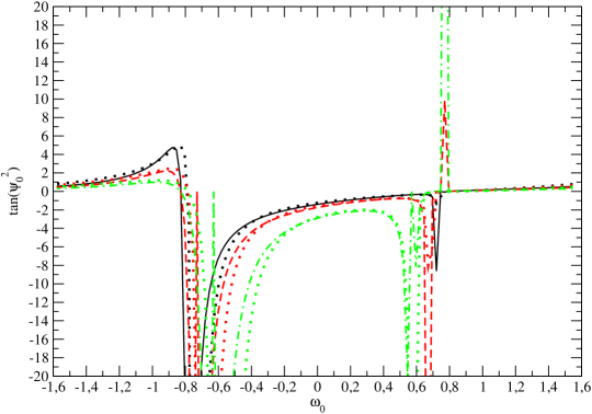
Figure 10: We show $\tan(\psi_{2})$ numerically obtained using eqns (76), (77), (79) and (80) after one iteration as a function of $\omega_{0}$ together with the corresponding results obtained by numerical solution of our equations of motion for the time period $\tau=4\tau_{*}$. $e_{0}=0.1$, $i_{0}=0.1$ for all shown cases. Solid, dashed and dot-dashed lines represent the results of the numerical solution for $\beta_{E}=5\cdot 10^{-3}$, $10^{-2}$ and $2\cdot 10^{-2}$, respectively, while the dotted lines are obtained using the map.

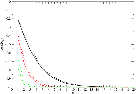
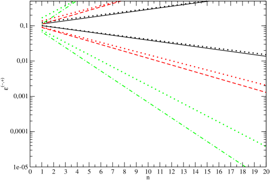
Figure 11: Top panel. The result of comparison of the map defined by eqns (76), (77), (79) and (80) with our analytic expressions. We show $\cos(2\psi_{0})$ numerically calculated with the help of the map as a function $n$, for $e_{0}=0.1$, $\psi_{0}(0)={3\pi\over 4}$, $i_{0}(0)=0.1$ and $\beta_{E}=5\cdot 10^{-3}$, $10^{-2}$ and $2\cdot 10^{-2}$ as solid, dashed and dot-dashed lines, respectively. Since $\sin(2\psi_{0}(0))<0$ for this case the appropriate analytic expressions are given by eq. (86). These are shown by dotted lines. Bottom panel. The evolution of $\epsilon^{\mp}$ for this case. The styles of the lines are for the same parameters as in top panel. The dotted curves are calculated according to eq. (88).

It is instructive to simplify the expressions (76), (77), (79) and (80) assuming that changes of the angles $\psi$ and $i$ during one cycle, $\Delta\psi=\psi_{2}-\psi_{1}$ and $\Delta i=i_{2}-i_{0}$ are small in comparison with the initial values. It is then straightforward to obtain

$$\Delta\psi=-{\beta_{E}\over 5i_{0}^{2}},\quad\Delta i=-i_{0}\cot(\psi_{0}){\Delta\Psi\over 2}.$$ (81)

From the conditions $|\Delta\psi|<1$ and $|\Delta i|/i_{0}<1$ we obviously have

$$\beta_{E}<\min(1,|\tan(\psi_{0})|)5i_{0}^{2}.$$ (82)

The condition (82) tells again that our approach is invalid when $\omega_{0}\approx\pi/4$, and, accordingly, $\psi_{0}\approx 0$.

Assuming that this condition holds we can extend the map (81) to many cycles by reducing it to ordinary differential equations according to the rule $\Delta\psi\rightarrow{d\psi_{0}\over dn}$ and $\Delta i\rightarrow{di_{0}\over dn}$, where $n$ is a number of cycles . Proceeding in this way we see that the second relation in eq. (81) can be immediately integrated and the result can be substituted in the first relation to give

$${d\psi_{0}\over dn}=-{\beta_{E}\over{i_{0}(0)}^{2}|\sin(2\psi_{0}(0))|}\sin(2\psi_{0}),\quad i_{0}=i_{0}(0)\sqrt{{|\sin(2\psi_{0}(0))|\over|\sin(2\psi_{0})|}},$$ (83)

where $i_{0}(0)$ and $\psi_{0}(0)$ are values of our variables in the beginning of the evolution corresponding to $n=0$. The first equation can be easily integrated with the result

$$\cos 2\psi_{0}={\cot^{2}(\psi_{0}(0))\exp({4\over 5}\phi_{E})-1\over\cot^{2}(\psi_{0}(0))\exp({4\over 5}\phi_{E})+1}\quad\phi_{E}={\beta_{E}n\over{i_{0}(0)}^{2}\sin(2\psi_{0}(0))}.$$ (84)

In the asymptotic limit of large $n$ we obtain from eq. (84) and the second expression in eq. (83)

$$\sin\psi_{0}\approx|\tan(\psi_{0}(0))|\exp(-{2\over 5}\phi_{E}),\quad\cos\psi_{0}\approx 1,\quad i_{0}\approx i_{0}(0)|\cos(\psi_{0}(0))|\exp({\phi_{E}\over 5})$$ (85)

when $\sin(2\psi_{0}(0))>0$ and

$$\cos\psi_{0}\approx|\cot(\psi_{0}(0))|\exp(-{2\over 5}|\phi_{E}|),\quad\sin\psi_{0}\approx 1,\quad i_{0}\approx i_{0}(0)|\sin(\psi_{0}(0))|\exp({|\phi_{E}|\over 5})$$ (86)

in the opposite case. Finally, we substitute eqns (85) and (86) in eq. (45) to obtain

$$\epsilon^{-}={i_{0}(0)|\sin\psi_{0}(0)|\over e_{0}^{1/5}}\exp(-{\phi_{E}\over 5}),\quad\epsilon^{+}={i_{0}(0)|\cos\psi_{0}(0)|\over e_{0}^{1/5}}\exp({\phi_{E}\over 5})$$ (87)

when $\sin(2\psi_{0}(0))>0$ and

$$\epsilon^{-}={i_{0}(0)|\sin\psi_{0}(0)|\over e_{0}^{1/5}}\exp({|\phi_{E}|\over 5}),\quad\epsilon^{+}={i_{0}(0)|\cos\psi_{0}(0)|\over e_{0}^{1/5}}\exp(-{|\phi_{E}|\over 5})$$ (88)

in the opposite case.

We compare our analytic results with the corresponding results based on the use of the map in Fig. 11. One can see a very good agreement between both approaches in the case when $\beta_{E}$ is sufficiently small $\sim<0.01$. For larger value of $\beta_{E}=2\cdot 10^{-2}$ the results are still in agreement, but it gets worse as expected.

References

- Komberg [1968] B. V. Komberg, Soviet Ast. 11, 727 (1968).
- Begelman et al. [1980] M. C. Begelman, R. D. Blandford, and M. J. Rees, Nature (London) 287, 307 (1980).
- Merritt and Milosavljevic [2005] D. Merritt and M. Milosavljevic, Living Reviews in Relativity 8, 8 (2005), arXiv:astro-ph/0410364 [astro-ph] .
- Komossa [2006] S. Komossa, Mem. Soc. Astron. Ital 77, 733 (2006).
- Gurvits et al. [2023] L. I. Gurvits, S. Frey, M. Krezinger, O. Titov, T. An, Y. Zhang, A. G. Polnarev, K. Gabanyi, K. Perger, and A. Melnikov, in The Multimessenger Chakra of Blazar Jets, IAU Symposium, Vol. 375, edited by I. Liodakis, M. F. Aller, H. Krawczynski, A. Lahteenmaki, and T. J. Pearson (2023) pp. 86–90, arXiv:2301.12283 [astro-ph.CO] .
- Valtonen et al. [2008] M. J. Valtonen et al., Nature (London) 452, 851 (2008), arXiv:0809.1280 [astro-ph] .
- Note [1] Note, however, that the SBBH model of OJ 287 with the standard parameters of the system was recently criticized both from observational and theoretical points of view, see [59] and [60], respectively.
- Grishchuk et al. [2001] L. P. Grishchuk, V. M. Lipunov, K. A. Postnov, M. E. Prokhorov, and B. S. Sathyaprakash, Physics Uspekhi 44, R01 (2001), arXiv:astro-ph/0008481 [astro-ph] .
- Amaro-Seoane et al. [2023] P. Amaro-Seoane et al., Living Reviews in Relativity 26, 2 (2023), arXiv:2203.06016 [gr-qc] .
- Auclair and al [2023] P. Auclair and al, Living Reviews in Relativity 26, 5 (2023), arXiv:2204.05434 [astro-ph.CO] .
- Ivanov et al. [2005a] P. B. Ivanov, A. G. Polnarev, and P. Saha, Monthly Notices of the Royal Astronomical Society 358, 1361–1378 (2005a).
- Zrake et al. [2025] J. Zrake, M. Clyburn, and S. Feyan, Mon. Not. R. Astron. Soc 10.1093/mnras/staf171 (2025), arXiv:2410.04961 [astro-ph.HE] .
- Blaes et al. [2002] O. Blaes, M. H. Lee, and A. Socrates, The Astrophysical Journal 578, 775–786 (2002).
- Hao et al. [2023] W. Hao, M. B. N. Kouwenhoven, R. Spurzem, P. A. Seoane, R. A. Mardling, and X. Xu, Analysis of kozai cycles in equal-mass hierarchical triple supermassive black hole mergers in the presence of a stellar cluster (2023), arXiv:2312.16986 [astro-ph.GA] .
- Merritt and Poon [2004] D. Merritt and M. Y. Poon, Astrophys. J 606, 788 (2004), arXiv:astro-ph/0302296 [astro-ph] .
- von Zeipel [1910] H. von Zeipel, Astronomische Nachrichten 183, 345 (1910).
- Lidov [1962] M. L. Lidov, Planet. Space Sci. 9, 719 (1962).
- Kozai [1962] Y. Kozai, Astron. J 67, 591 (1962).
- Ito and Ohtsuka [2019] T. Ito and K. Ohtsuka, Monographs on Environment, Earth and Planets 7, 1 (2019), arXiv:1911.03984 [astro-ph.EP] .
- Chen et al. [2020] Y. Chen, Q. Yu, and Y. Lu, Astrophys. J 897, 86 (2020), arXiv:2005.10818 [astro-ph.HE] .
- Sesana [2010] A. Sesana, The Astrophysical Journal 719, 851–864 (2010).
- Iwasawa et al. [2011] M. Iwasawa, S. An, T. Matsubayashi, Y. Funato, and J. Makino, Astrophys. J., Lett 731, L9 (2011), arXiv:1011.4017 [astro-ph.GA] .
- Fiestas et al. [2012] J. Fiestas, O. Porth, P. Berczik, and R. Spurzem, Mon. Not. R. Astron. Soc 419, 57 (2012), arXiv:1108.3993 [astro-ph.GA] .
- Wang et al. [2014] L. Wang, P. Berczik, R. Spurzem, and M. B. N. Kouwenhoven, Astrophys. J 780, 164 (2014), arXiv:1311.4285 [astro-ph.GA] .
- Khan et al. [2020] F. M. Khan, M. A. Mirza, and K. Holley-Bockelmann, Mon. Not. R. Astron. Soc 492, 256 (2020), arXiv:1911.07946 [astro-ph.GA] .
- Berczik et al. [2022] P. Berczik, M. Arca Sedda, M. Sobolenko, M. Ishchenko, O. Sobodar, and R. Spurzem, å 665, id.A86 (2022).
- Vasiliev et al. [2015] E. Vasiliev, F. Antonini, and D. Merritt, The Astrophysical Journal 810, 49 (2015).
- Lezhnin and Vasiliev [2019] K. Lezhnin and E. Vasiliev, Mon. Not. R. Astron. Soc 484, 2851 (2019), arXiv:1901.04508 [astro-ph.GA] .
- Note [2] Let us stress that the symmetries of the stellar distribution correspond to its initial state, since they are broken to some extent after a SBBH starts to evolve within a stellar cluster.
- Chandrasekhar [1969] S. Chandrasekhar, Ellipsoidal figures of equilibrium (1969).
- Ivanov and Papaloizou [2011] P. B. Ivanov and J. C. B. Papaloizou, Celestial Mechanics and Dynamical Astronomy 111, 51 (2011), arXiv:1106.5753 [astro-ph.EP] .
- Note [3] Note that when density perturbations are small, the explicit form of can be found e.g. in [61].
- Ivanov et al. [2005b] P. B. Ivanov, A. G. Polnarev, and P. Saha, Mon. Not. R. Astron. Soc 358, 1361 (2005b), arXiv:astro-ph/0410610 [astro-ph] .
- Petrovich and Antonini [2017] C. Petrovich and F. Antonini, The Astrophysical Journal 846, 146 (2017).
- Hamilton and Rafikov [2019a] C. Hamilton and R. R. Rafikov, Mon. Not. R. Astron. Soc 488, 5489 (2019a), arXiv:1902.01344 [astro-ph.GA] .
- Hamilton and Rafikov [2019b] C. Hamilton and R. R. Rafikov, Mon. Not. R. Astron. Soc 488, 5512 (2019b), arXiv:1902.01345 [astro-ph.SR] .
- Hamilton and Rafikov [2021] C. Hamilton and R. R. Rafikov, Mon. Not. R. Astron. Soc 505, 4151 (2021), arXiv:2011.14947 [astro-ph.GA] .
- Georgiev et al. [2016] I. Y. Georgiev et al., Mon. Not. R. Astron. Soc 457, 2122 (2016), arXiv:1601.02613 [astro-ph.GA] .
- Young [1980] P. Young, Astrophys. J 242, 1232 (1980).
- Note [4] We remind that is also often denoted as the orbital angular frequency, is defined as the inclination angle of the orbital plane with respect to the symmetry plane of the problem, defines the position of the intersection line of the orbital and symmetry planes in the symmetry plane, and defines the position of the orbital periastron with respect to the intersection line, see e.g. https://en.wikipedia.org/wiki/OrbitalnodeNodedistinction for a graphical representation.
- Murray and Dermott [1999] C. D. Murray and S. F. Dermott, Solar System Dynamics (1999).
- Landau and Lifshitz [1975] L. D. Landau and E. M. Lifshitz, The classical theory of fields (1975).
- Merritt [2013] D. Merritt, Dynamics and Evolution of Galactic Nuclei (2013).
- Note [5] Note that it is qualitatively different from the case , where remains to be zero during the evolution, see eq. (12).
- Note [6] Let us stress that the choice to to be equal to either (-) or (+) is independent from the choice of during the stages when is either close to zero or . In the former case we use , while in the latter case we show explicitly in all appropriate equations.
- Note [7] Here and in eqns (41) and (42) we take into account that the change of from to takes place when and the opposite change corresponds to .
- Note [8] Note that although only one set of the initial values of our dynamical variables is represented we have checked that a similar situation takes place when other sets are used.
- Note [9] We remind that we always set initial value of the apsidal angle to be equal to the negative of the nodal angle.
- Peters [1964] P. C. Peters, Physical Review 136, 1224 (1964).
- Cutler et al. [1994] C. Cutler, D. Kennefick, and E. Poisson, Phys. Rev. D 50, 3816 (1994).
- Flanagan and Hinderer [2007] E. Flanagan and T. Hinderer, Phys. Rev. D 75, 124007 (2007), arXiv:0704.0389 [gr-qc] .
- Mino [2003] Y. Mino, Phys. Rev. D 67, 084027 (2003), arXiv:gr-qc/0302075 [gr-qc] .
- Merritt and Vasiliev [2011] D. Merritt and E. Vasiliev, Astrophys. J 726, 61 (2011), arXiv:1005.0040 [astro-ph.GA] .
- Note [10] Using eqns (20) of IPS (Note a misprint in denominator of the first equation, there should be instead of .), setting there and assuming, for simplicity, that and are small, we easily obtain the minimal eccentricity , where as before corresponds to the minimal eccentricity . Thus, contrary to our case small values of can only be obtained for . In this approximation the angle corresponding to the smallest is approximately equal to .
- Tomar et al. [2024] Y. Tomar, C. Dinh, G. Li, and D. Lin, Mon. Not. R. Astron. Soc 534, 1329 (2024).
- Arun et al. [2008] K. G. Arun, L. Blanchet, B. R. Iyer, and M. S. S. Qusailah, Phys. Rev. D 77, 064035 (2008), arXiv:0711.0302 [gr-qc] .
- Gopakumar and Iyer [1997] A. Gopakumar and B. R. Iyer, Phys. Rev. D 56, 7708 (1997), arXiv:gr-qc/9710075 [gr-qc] .
- Note [11] Remembering that the time period of one cycle is , it possible to use the time as an independent variable instead of with the help of substitution .
- Komossa et al. [2023] S. Komossa et al., Mon. Not. R. Astron. Soc 522, L84 (2023), arXiv:2302.11646 [astro-ph.HE] .
- Ivanov and Zhuravlev [2024] P. B. Ivanov and V. V. Zhuravlev, Mon. Not. R. Astron. Soc 528, 337 (2024), arXiv:2401.01317 [astro-ph.GA] .
- Binney and Tremaine [1987] J. Binney and S. Tremaine, Galactic dynamics (1987).