Finite Pinwheel Scheduling: the k-Visits Problem

Abstract

Pinwheel Scheduling is a fundamental scheduling problem, in which each task $i$ is associated with a positive integer $d_{i}$, and the objective is to schedule one task per time slot, ensuring each task perpetually appears at least once in every $d_{i}$ time slots. Although conjectured to be PSPACE-complete, it remains open whether Pinwheel Scheduling is NP-hard (unless a compact input encoding is used) or even contained in NP.

We introduce $k$-Visits, a finite version of Pinwheel Scheduling, where given $n$ deadlines, the goal is to schedule each task exactly $k$ times. While we observe that the $1$-Visit problem is trivial, we prove that $2$-Visits is strongly NP-complete through a surprising reduction from Numerical 3-Dimensional Matching (N$3$DM). As intermediate steps in the reduction, we define NP-complete variants of N$3$DM which may be of independent interest. We further extend our strong NP-hardness result to a generalization of $k$-Visits ($k\geq 2$) in which the deadline of each task may vary throughout the schedule, as well as to a similar generalization of Pinwheel Scheduling, thus making progress towards settling the complexity of Pinwheel Scheduling.

Additionally, we prove that $2$-Visits can be solved in linear time if all deadlines are distinct, rendering it one of the rare natural problems which exhibit the interesting dichotomy of being in P if their input is a set and NP-complete if the input is a multiset. We achieve this through a Turing reduction from $2$-Visits to a variation of N$3$DM, which we call Position Matching. Based on this reduction, we also show an FPT algorithm for $2$-Visits parameterized by a value related to how close the input deadlines are to each other, as well as a linear-time algorithm for instances with up to two distinct deadlines.

1 Introduction

Deadline-based scheduling problems are fundamental in both theory and practice, arising in diverse settings such as manufacturing, communications, satellite operations and are even present in everyday tasks. For example, imagine a single delivery truck tasked with supplying several stores, each with diverse restocking needs. The challenge is to figure out a schedule that ensures all stores are resupplied before running out of stock. How can the truck manage this, given the varying demands of each store?

The Pinwheel Scheduling problem [24] (also known as Windows Scheduling with one channel [3, 4], or Periodic Scheduling, e.g. [2]) formalizes such questions in perpetual settings as follows. Given a multiset $D=\{d_{1},\ldots,d_{n}\}$ of positive integers (deadlines), the goal is to determine whether there exists an infinite sequence over $\{1,\ldots,n\}$ such that any subsequence of $d_{i}$ consecutive entries contains at least one instantiation of $i$. Despite its simple description, this problem still has many open questions, with its complexity in particular remaining open for over three decades. Although conjectured to be PSPACE-complete, NP-hardness has only been proven when the multiplicity of each deadline is given as input (compact encoding). Very little is known when the input is given explicitly as a multiset (see Table 1). Note that instances with sum of inverse deadlines (density) greater than $1$ do not admit a feasible schedule. In a recent breakthrough, Kawamura [27] also proved that instances with density not exceeding $5/6$ always admit a feasible schedule, which was a long-standing conjecture proposed by [9].

	Pinwheel Scheduling	2-Visits (our results)
Feasible when density $\leq 5/6$	Always [9, 27]	Always
Feasible when density $>1$	Never [24]	Sometimes
Complexity (explicit input)	In PSPACE [24]	Strongly NP-complete
	Conjectured PSPACE-complete [7]	In P for distinct deadlines
	Unknown whether NP-hard
	Unknown whether in NP
	Pseudopoly-time unlikely [26]
	In NP when Density $=1$ [24]
Complexity (compact input)	NP-hard [24, 4]	Strongly NP-complete
	Unknown whether in NP
Tractable special cases	Two distinct numbers [25]	Two distinct numbers
	Three distinct numbers [29]	All deadlines distinct
		Bounded cluster size

Table 1: Our results for 2-Visits compared to their Pinwheel Scheduling counterparts.

In this work, we introduce a finite variant of Pinwheel Scheduling, which we call $k$-Visits. The motivation for this variant is twofold: first, certain deadline-based applications may only require a finite amount of task repetitions; second, the study of this variant may be useful as an intermediate step for settling the complexity of Pinwheel Scheduling. Notably, the proof of PSPACE-membership of Holte et al. [24] implies that the existence of an infinite schedule is equivalent to the existence of a (finite) schedule of length equal to the product of the input deadlines, strengthening the connection between finite and infinite variants of the problem.

We find that the simplest version of $k$-Visits in which $k=1$ is trivial, but the $k=2$ version turns out to be a challenging combinatorial problem. Hence, the main focus of this work is the $k=2$ version, i.e., the $2$-Visits problem, for which we prove strong NP-completeness and propose special-case polynomial-time algorithms. Notably, this strong NP-hardness result transfers to a generalization of Pinwheel Scheduling in which the deadline of each task may vary throughout the schedule. This is of particular interest as, to the best of our knowledge, no such result exists for Pinwheel Scheduling. We summarize the main differences in what is known for the two problems in Table 1.

1.1 Related Work

Holte et al. [24] introduced the Pinwheel Scheduling problem, proving that it is contained in PSPACE by reducing any infinite schedule to a finite one. In the same paper, the authors introduce the concept of density and prove membership in NP when restricted to instances with density equal to $1$, while also claiming NP-hardness for compact input (see [4] for a proof). Ever since the problem’s introduction, it has remained open whether it is contained in NP or is NP-hard (for explicit input), despite the conjecture of PSPACE-completeness [7]. Regardless, it has been used to classify the complexity of certain inventory routing problems [1]. To the best of our knowledge, the most relevant complexity result for Pinwheel Scheduling appears in [26], where it is claimed that it does not admit a pseudo-polynomial time algorithm under reasonable assumptions.

Since Pinwheel Scheduling is conjectured to be hard, there have been various attempts to determine easy special cases. Variants with a bounded amount of distinct deadlines have been studied in [24, 25, 29]. Additionally, there exists a substantial line of research proving that feasible schedules always exist when the density of the input is bounded by some constant. Holte et al. [24] gave the first such bound of $0.5$; Bar-Noy et al. [4], Chan and Chin [9, 8], Fishburn and Lagarias [19] all improved this bound, with [9] conjecturing that the bound can be improved up to $5/6$. Gasieniec et al. [22] recently proved the $5/6$-conjecture for instances of size at most $12$. In a recent breakthrough paper, Kawamura [27] finally proved the conjecture in the general setting.

There is also extensive bibliography for variations and generalizations of Pinwheel Scheduling. For example, [17] studies a variant in which each task additionally has a duration, and [28] studies a variant with multiple agents. Bamboo Garden Trimming (BGT) [21] is a closely related optimization problem (see also [15, 16, 23]), in which one bamboo is trimmed at a time in a garden of bamboos growing with different rates and the objective is to minimize the maximum height. The state-of-the-art approximation algorithm for BGT seems to be the one in [27], given as a corollary of the density threshold conjecture. A generalization of BGT is studied in [5].

In addition to the scheduling-based approach, another line of research addresses the problem through a graph-theoretic perspective, where the objective is to visit every node of a graph with a certain frequency. The most basic form of this problem in which each node must be visited once is known as Exploration [30] (for a survey see [14]). An extension of the Exploration problem, where each node must be visited within specific time constraints, is studied in [12]. In the case where each node of the graph needs to be repeatedly visited, the problem is known as Perpetual Exploration (e.g., [6]) or Patrolling (for a recent survey see [11]). The most relevant variation of Patrolling to our work is known as Patrolling with Unbalanced Frequencies [10], in which the objective is to satisfy constraints on the maximum allowable time between successive visits to the same node. However, results in that context focus on continuous lines (e.g., [10, 13]) and on multiple agents (e.g., [13]), whereas our setting is analogous to complete graphs and a single agent.

1.2 Our Contribution

We introduce a finite variant of the classical Pinwheel Scheduling problem, which we call $k$-Visits. This problem can be modeled by an agent traversing a complete graph with loops, with each node having a deadline and the goal being to visit each node exactly $k$ times without its deadline expiring between consecutive visits. While we observe that $1$-Visit is solvable by a trivial algorithm, we find that $2$-Visits is a challenging combinatorial problem. In particular, our main result establishes that $2$-Visits is strongly NP-complete, even when deadlines are given explicitly. This is in contrast to the current status of Pinwheel Scheduling, which is not known to be NP-hard when the input is explicit and not known to be strongly NP-hard under any input encoding. Our main result implies strong NP-hardness for a generalization of Pinwheel Scheduling in which the deadline of each node may change once throughout the schedule. We thus make significant progress towards understanding the computational complexity of Pinwheel Scheduling and other deadline-based scheduling problems. All hardness results in this paper concern explicit input encoding and, thus, also hold for compact encoding.

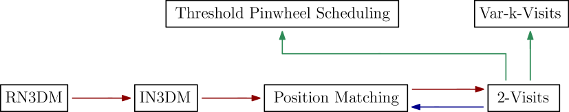
Figure 1: A map of our reductions. RN3DM (Def. 12) and IN3DM (Def. 11) are variants of Numerical 3-Dimensional Matching. Reductions denoted by red arrows are used to prove strong NP-completeness for 2-Visits (Section 5). The blue-arrow reduction is a linear time Turing reduction from 2-Visits to Position Matching, and is the backbone of the algorithms we propose for $2$-Visits (Section 4). Lastly, the green-arrow reductions prove strong NP-hardness for generalizations of $k$-Visits and Pinwheel Scheduling (Section 6).

A more detailed description of our hardness results follows. We prove strong NP-completeness for $2$-Visits via a surprising chain of reductions starting from a variation of Numerical 3-Dimensional Matching (N3DM) defined in [31], and then transfer this hardness result to generalizations of $k$-Visits ($k\geq 2$) and Pinwheel Scheduling. As intermediate steps in our reductions, we define NP-complete variations of N3DM which may be of independent interest. In particular, we introduce a severely restricted variation of N3DM, which we call Position Matching, serving as a key component in our results. Our reductions are summarized in Figure 1. A major technical challenge stems from the constraints of Position Matching and particularly from the concept of discretized sequences (see Def. 5) which is fundamental for our definitions.

Despite the intractability of $2$-Visits, we identify tractable special cases through a linear-time Turing reduction from $2$-Visits to Position Matching. Specifically, we present linear-time algorithms when all deadlines are distinct or when there are at most two distinct deadlines. This leads to an interesting dichotomy: our hardness result for $2$-Visits holds when the input is a multiset, but the problem can be solved in linear time when the input is a simple set. This sensitivity to input multiplicity is rare for natural problems and highlights an interesting structural boundary in the complexity landscape of deadline-based problems. Additionally, we provide an FPT algorithm parameterized by the maximum cluster size (see Definitions 5, 9); intuitively, this is a parameter related to how close the input deadlines are to each other.

Our paper is structured as follows. In Section 3, we give a brief overview of the $1$-Visit problem. In Section 4 we study various properties of $2$-Visits schedules, leading to special-case polynomial-time algorithms for the problem. In Section 5, we prove strong NP-completeness for $2$-Visits, which we consider our main technical contribution. Finally, in Section 6 we extend our hardness result to generalizations of $k$-Visits ($k\geq 2$) and of Pinwheel Scheduling. We stress that Section 4 (Theorems 1 and 2 in particular) provides intuition for the connection between $2$-Visits and Position Matching, which is necessary to understand our main result in Section 5.

2 Preliminaries and problem definition

2.1 Preliminaries

We use the notations $[n]=\{1,\dots,n\}$ and $[m,n]=\{m,\ldots,n\}$ for positive integers $m\leq n$.

Definition 1 (Pinwheel Scheduling [24]).

Given a non-decreasing sequence of $n$ positive integers (deadlines) $d_{i}$, $i\in[n]$, the Pinwheel Scheduling problem asks whether there exists an infinite schedule $p_{1},p_{2},\ldots$ , where $p_{j}\in[n]$ for $j\in\mathbb{N}$, such that for all $i\in[n]$ any $d_{i}$ consecutive entries contain at least one occurrence of $i$.

Definition 2 (Density).

For a non-decreasing sequence of $n$ positive integers (deadlines) $d_{i}$, $i\in[n]$, we define its density as $\sum_{i=1}^{n}1/d_{i}$.

Definition 3 (N3DM).

Given three multisets of positive integers $A=\{a_{1},\ldots,a_{n}\}$, $B=\{b_{1},\ldots,b_{n}\}$, $C=\{c_{1},\ldots,c_{n}\}$ and an integer $\sigma$ such that

$$\sum_{i=1}^{n}(a_{i}+b_{i}+c_{i})=n\sigma,$$

the Numerical 3-Dimensional Matching $(\textnormal{{N3DM}})$ problem asks whether there is a subset $M$ of $A\times B\times C$ s.t. every $a_{i}\in A$, $b_{i}\in B$, $c_{i}\in C$ occurs exactly once in $M$ and for every triplet $(a,b,c)\in M$ it holds that $a+b+c=\sigma$.

N3DM is a variation of the classic strongly NP-complete problem 3-Partition and is also strongly NP-complete [20]. We will use variations of N3DM for our reductions.

2.2 The $k$-Visits problem

Definition 4 ($k$-Visits).

Given a non-decreasing sequence of $n$ positive integers (deadlines) $d_{i}$, $i\in[n]$, the $k$-Visits problem asks whether there exists a schedule of length $nk$, containing each $i\in[n]$ exactly $k$ times, with the constraint that every occurrence of $i$ is at most $d_{i}$ positions away from the previous one (or from the beginning of the schedule, if it is the first one).

The $k$-Visits problem can be modeled by an agent traversing a complete graph with loops where all edges have weight $1$ and each node $i$ has a deadline $d_{i}$. In each time unit, the agent can traverse an edge and renew the deadline of the node it visits, with the goal being to visit each node a total of $k$ times without its deadline expiring. With this in mind, we will refer to the numbers $i\in[n]$ as nodes throughout the paper.

Observation 1.

If a sequence of $n$ positive integers does not have a feasible schedule for the $k$-Visits problem, then it does not have a feasible schedule for any $k^{\prime}\textnormal{{-Visits}}$ problem with $k^{\prime}>k$. Moreover, it has no feasible schedule for Pinwheel Scheduling, which can (informally) be seen as the $\infty\textnormal{{-Visits}}$ problem.

Corollary 1.

A $k$-Visits instance with density not exceeding $5/6$ admits a feasible schedule, due to the density threshold conjecture proven for Pinwheel Scheduling in [27].

Observation 2.

The inverse of Observation 1 does not hold. Notably, sequences with density exceeding $1$ may have a feasible schedule for $k$-Visits (for some positive integer $k$), even though they never have a feasible schedule for Pinwheel Scheduling [24].

The following definition will prove crucial for studying the $k$-Visits problem.

Definition 5 (Discretized Sequence).

Given a non-decreasing sequence $D=\langle d_{1},\ldots,d_{n}\rangle$ of positive integers, we define its discretized sequence $A=\langle a_{1},\ldots,a_{n}\rangle$ as follows.

$$a_{i}=\begin{cases}d_{i},\ i=n\\ \min\{a_{i+1}-1,d_{i}\},\ i<n\end{cases}$$

Intuitively, the discretized sequence of a sequence of deadlines $d_{i}$ contains the latest possible positions in which the first visits of all $n$ nodes can occur. For example, the discretized sequence of $\langle 6,8,8,8,11,11,14\rangle$ is $\langle 5,6,7,8,10,11,14\rangle$. A discretized sequence can be computed in $\mathcal{O}(n)$ time.

Throughout the paper, we may refer to the input of $k$-Visits as a multiset instead of a sequence, when it is more convenient (or a set, if it does not contain duplicates). For 2-Visits specifically (which is the main focus of this paper), we will use the following definition.

Definition 6 (2-Visits).

Given a non-decreasing sequence of $n$ positive integers (deadlines) $d_{i}$, $i\in[n]$, the 2-Visits problem asks whether there exists a schedule of length $2n$, containing a primary and a secondary visit for each $i\in[n]$. For every $i\in[n]$, its primary visit must be at most $d_{i}$ positions away from the beginning of the schedule and its secondary visit must be either before its primary visit or at most $d_{i}$ positions after its primary visit.

Note that Def. 6 is equivalent to Def. 4 for $k=2$ and will significantly simplify many of our proofs by allowing a secondary visit to appear before the respective primary visit (in contrast to using first and second visits).

3 The 1-Visit problem

Lemma 1.

If a 1-Visit instance $\langle d_{1},d_{2},\ldots,d_{n}\rangle$ has a feasible schedule, then the schedule $1,2,\ldots,n$ is feasible for this instance.

Proof.

Let us assume that a feasible schedule $S^{\prime}$ exists and that the schedule $S=1,2,\ldots,n$ is not feasible. Let $p$ be the first position where $S$ and $S^{\prime}$ differ. Let $i$ be the node in position $p$ of $S$, $j$ the node in position $p$ of $S^{\prime}$ and $p^{\prime}>p$ be the position of $S^{\prime}$ where node $i$ is placed. Then, $i$ and $j$ can be swapped in $S^{\prime}$, as by definition $d_{i}<d_{j}$. Iteratively, the same swapping argument holds for every position where $S$ and $S^{\prime}$ differ and, as a result, $S^{\prime}$ can be transformed to $S$ without violating a deadline at any step. Therefore $S$ is also a feasible schedule, contradiction. ∎

Lemma 2.

A 1-Visit instance has a feasible schedule if and only if the discretized sequence of the input contains only (strictly) positive elements.

The proof of this lemma follows immediately from Lemma 1 and Def. 5, and is thus omitted.

Corollary 2.

1-Visit can be solved in $\mathcal{O}(n)$ time.

4 Polynomial-time algorithms for special cases of 2-Visits

Trivial algorithms, such as greedily visiting the node with minimum deadline, fail for the 2-Visits problem. In fact, as we will see later, there are instances of 2-Visits where neither the first nor the second visits appear in order of non-decreasing deadline in any feasible schedule.

Definition 7 (Induced deadline).

For a node $i$ whose primary visit occurs in position $t_{i}$ of a schedule, we define its induced deadline as $d_{i}^{\prime}=d_{i}+t_{i}$. Intuitively, this number dictates the latest position in which the secondary visit of node $i$ is allowed to occur.

A key intuition for any algorithm is to push primary visits as late as possible to maximize the induced deadlines. This intuition, although crucial, is insufficient for solving the 2-Visits problem. It turns out that, for certain instances, the primary visits must be permuted in a counterintuitive manner in order to allow a feasible schedule. This is demonstrated in the following example.

Example 1.

Let $\langle 4,5,6,7,8,8,10,10,11,15,22,23\rangle$ be a 2-Visits instance. One can observe that it is impossible to construct a feasible schedule for this instance by choosing primary visits in non-decreasing order. This happens because nine primary visits must be done until time unit $11$, leaving space for only two secondary visits until that time unit. A reasonable choice is to visit the first two nodes twice each as early as possible; however, this would only make the induced deadline of the third node equal to $11$, which causes a problem because there is already a primary visit that must be placed at position $11$. A correct order of primary visits is actually $4,5,8,6,7,8,10,10,11,15,22,23$; it is not hard to verify that there exists a feasible schedule respecting this order.

At first glance, the aforementioned permutation of primary visits in Example 1 seems somewhat arbitrary. Surprisingly, every feasible schedule of that instance requires the nodes with deadlines $6,7,8,8$ to be visited in the order $8,6,7,8$. In order to systematically study permutations of primary visits, we will later introduce the Position Matching problem, which serves as a key component of both our algorithms and hardness results.

4.1 Properties of feasible 2-Visits schedules

In the proofs of this subsection we will transform feasible schedules to make them satisfy certain useful properties, thus greatly limiting the amount of schedules that have to be considered by a 2-Visits algorithm. By Lemma 2, an input with a discretized sequence containing a non-positive number cannot have a feasible schedule for 1-Visit, and thus neither for 2-Visits (by Obs. 1). From now on, we assume that the input always has a discretized sequence of positive numbers. We will also assume that the input contains no deadlines greater than $2n$. If it does, then the respective node would never expire and, thus, its two visits can be placed at the last two positions of the schedule. Clearly, a feasible schedule exists if and only if the input minus that node has a feasible schedule.

Definition 8 (Gap).

Let $A$ be the discretized sequence of a 2-Visits instance. We call a position $i\in[2n]$ a gap if $i\notin A$.

With the above assumptions, any 2-Visits instance has exactly $n$ gaps in $[2n]$. In Example 1, the discretized sequence is $\langle 3,4,5,6,7,8,9,10,11,15,22,23\rangle$; hence, the $n=12$ gaps of this instance are $\{1,2,12,13,14,16,17,18,19,20,21,24\}$.

A key idea that we will use in our approach is that placing all primary visits in the positions dictated by the discretized sequence is, in a certain sense, the best choice for obtaining a schedule. This crucial observation is formalized in Lemma 5 and will play a major role for the algorithms we propose in this section, as well as for the proof of strong NP-completeness of 2-Visits in Section 5.

Before stating Lemma 5, we prove two auxiliary lemmas.

Lemma 3.

Let $A=\langle a_{1},\ldots,a_{n}\rangle$ be the discretized sequence of a 2-Visits instance $D=\langle d_{1},\ldots,d_{n}\rangle$. For any $i\in[n]$ it holds that at most $n-i$ primary visits can occur after position $a_{i}$.

Proof.

We use induction on $i$, with $i=n$ as base.

Basis $(i=n)$. We have $d_{n}=a_{n}$, hence no primary visit may occur after position $a_{n}$.

Inductive step $(i<n)$. Suppose that at most $n-i-1$ primary visits occur after position $a_{i+1}$. By Def. 5, we need to consider the following two cases.

Case 1: $a_{i}=a_{i+1}-1$. Since $a_{i},\ a_{i+1}$ are consecutive positions, it follows immediately from the induction hypothesis that at most $n-i$ primary visits can occur after $a_{i}$.

Case 2: $a_{i}=d_{i}$. Primary visits of nodes $j\leq i$ cannot be placed after position $a_{i}$, since $d_{j}\leq d_{i}=a_{i}$. Hence, at most $n-i$ primary visits can occur after $a_{i}$. ∎

Lemma 4.

If a feasible schedule places some secondary visit in a non-gap position $p$, then there exists some primary visit in a position $q<p$ belonging to a node $u$ with $d_{u}\geq p$.

Proof.

Since $p$ is not a gap, it holds that $p\in A$. Suppose $p$ is the $i$-th element of $A$, i.e., $p=a_{i}$. By Lemma 3, there are at least $i$ primary visits before position $p$ (not including $p$, by assumption). By the pigeonhole principle, one of these must have deadline at least $d_{i}$. By Def. 5, $p=a_{i}\leq d_{i}$. ∎

Lemma 5.

If a 2-Visits instance has a feasible schedule, then it has a feasible schedule in which all secondary visits are placed in gaps (equivalently: no primary visit is placed in a gap).

Proof.

Suppose we have a feasible schedule which places the secondary visit of some node $v$ in a non-gap position $p$. By Lemma 4, there is a primary visit in a position $q<p$ belonging to a node $u$ with $d_{u}\geq p$. This allows us to swap the entries in positions $q,\ p$ without affecting the feasibility of the schedule; the primary visit of $u$ can be placed in position $p$, since $d_{u}\geq p$, and the secondary visit of $v$ is moved to an earlier position, preserving feasibility. Note that this argument holds even if $v=u$.

If by the above modification $v$ was again placed in a non-gap position, we can apply Lemma 4 iteratively and do the same modification. Note that this modification moves the secondary visit of $v$ to an earlier position, therefore it can only be applied a finite number of times. This implies that this procedure will terminate at some point, i.e., $v$ will be placed in a gap.

We can apply this procedure to all nodes $v$ whose secondary visits are not in gaps. Note that the procedure never displaces secondary visits that have been placed in gaps, therefore, by doing this, we will end up with a feasible schedule satisfying the desired property. ∎

We now present the main theorem of this subsection.

Theorem 1.

If a 2-Visits instance has a feasible schedule, then it has a feasible schedule in which:

1. All secondary visits are placed in gaps. (Equivalently: no primary visit is placed in a gap.)

2. Secondary visits appear in the schedule in order of non-decreasing induced deadlines.

Proof.

By Lemma 5, we know that there is a feasible schedule satisfying the first property. Take such a schedule and reorder its secondary visits by non-decreasing induced deadline (primary visit positions are not affected by this modification). We can prove that the new schedule is also feasible through swapping arguments similar to the proof of Lemma 1 (using induced deadlines instead of simple deadlines). ∎

4.2 Reducing 2-Visits to Position Matching

Definition 9 (Cluster).

We call a maximal subsequence of consecutive numbers of the discretized sequence of a 2-Visits instance a cluster. For two cluster $C_{1},\ C_{2}$ of a discretized sequence, we say that $C_{1}$ precedes $C_{2}$ if the elements of $C_{1}$ are smaller than the elements of $C_{2}$.

Example 2.

Consider input $D=\langle 6,8,8,8,11,11,14\rangle$ with $n=7$. Then, $A=\langle 5,6,7,8,10,11,14\rangle$ is made up of three clusters: $C_{1}=\langle 5,6,7,8\rangle$, $C_{2}=\langle 10,11\rangle$ and $C_{3}=\langle 14\rangle$. Every $i\in[2n]$ that is not in any of these clusters is a gap.

Observation 3.

If $\langle a_{p},\ldots,a_{q}\rangle$ is a cluster, then it is the discretized sequence of $\langle d_{p},\ldots,d_{q}\rangle$. For example, $C_{1}=\langle 5,6,7,8\rangle$ is the discretized sequence of $\langle 6,8,8,8\rangle$ in Example 2. Similarly, $C_{2}=\langle 10,11\rangle$ is the discretized sequence of $\langle 11,11\rangle$. The reason that this property holds is that $d_{q}=a_{q}$, by Definitions 5, 9.

Lemma 6.

Let $\langle a_{i},\ldots,a_{j}\rangle$ be a cluster of the discretized sequence $A$ of a 2-Visits input. For any feasible schedule that satisfies the properties of Theorem 1, it holds that the primary visits of nodes $i,\ldots,j$ are placed in some permutation of the positions in $\langle a_{i},\ldots,a_{j}\rangle$.

Proof.

If $A$ consists of only one cluster, then the lemma follows immediately from Theorem 1. Assume $A$ consists of more than one cluster.

Let $F$ be a feasible schedule that satisfies the properties of Theorem 1 and let $C_{1}=\langle a_{1},\ldots,a_{m}\rangle$ be the first cluster of $A$. Since $C_{1}$ is a cluster, it holds that $a_{m}<a_{m+1}-1$. By Def. 5, this implies that $a_{m}=d_{m}$ and, thus, $d_{m}<a_{m+1}-1$. Since $D=\langle d_{1},\ldots,d_{n}\rangle$ is a non-decreasing sequence, we obtain that:

$$d_{i}<a_{m+1}-1,\ \forall i\in[m]$$ (1)

Recall that in a schedule satisfying the properties of Theorem 1, no primary visit is in a gap. Thus, all primary visits must be placed at some $a_{i}\in A$. By (1), we know that the first $m$ primary visits cannot be placed in $a_{m+1}$ or later. Thus, all of them must be placed in some permutation of the positions $a_{1},\ldots,a_{m}$.

We can prove the lemma through induction, using the above proof for $C_{1}$ as the induction basis. In each step, we study a cluster $C_{j}=\langle a_{p},\ldots,a_{q}\rangle$. By induction hypothesis, we know that all $a_{i},\ i\in[p-1]$, are occupied by primary visits of nodes $i\in[p-1]$. Exactly the same arguments apply to show that primary visits of nodes $i\in[p,q]$ cannot be placed in any position greater than $a_{q}$, thus forcing them to be placed in some permutation of the positions in $\langle a_{p},\ldots,a_{q}\rangle$, which completes the proof. ∎

By Theorem 1 and Lemma 6, we know that in order to find a feasible schedule, it suffices to:

• Place the primary visits of nodes corresponding to each cluster in some permutation of the positions of that cluster.

• Place secondary visits in gaps in order of non-decreasing induced deadline.

A brute force algorithm based on this information would run in time $\mathcal{O}(n!)$, if all $n$ elements of the discretized sequence form a cluster. In order to investigate whether this complexity can be improved, we introduce the Position Matching problem, which captures the question of how primary visits should be permuted (see Theorem 2).

Definition 10 (Position Matching).

Given a non-decreasing sequence $D=\langle d_{1},\ldots,d_{n}\rangle$ of positive integers, its discretized sequence $A=\langle a_{1},\ldots,a_{n}\rangle$ and a set $T=\{t_{1},\ldots,t_{n}\}$ of $n$ distinct positive integers (targets), the Position Matching problem asks whether there is a subset $M$ of $D\times A\times T$ s.t. every $d_{i}\in D$, $a_{i}\in A$, $t_{i}\in T$ occurs exactly once in $M$ and for every triplet $(d,a,t)\in M$ it holds that $d\geq a$ and $d+a\geq t$.

We would like to emphasize the restriction that elements of $D$ cannot be matched with larger elements of $A$. Throughout the paper, we will say that a tuple $(d,a)$ satisfies a target $t$ if $d+a\geq t$.

Example 3.

Let $D=\langle 6,7,8,8,15,15\rangle$ and $T=\{12,13,14,15,20,28\}$. We compute the discretized sequence $A=\langle 5,6,7,8,14,15\rangle$ of $D$. A solution to this Position Matching instance consists of the following $D$-$A$ pairs: $(6,6),(8,5),(7,7),(8,8),(15,14),(15,15)$. The sums of these pairs are $12,13,14,16,29,30$, satisfying all targets.

Remark 1.

Although $A$ can be derived from $D$ in Def. 10, we assume it is given as input for the sake of readability. In general, throughout the paper, whenever a variant of N3DM is discussed we consider all three sets as input, even if some of them can be implicitly derived. This makes our reductions in the next section more natural and easier to read.

Lemma 7.

Let $C_{1}$ and $C_{2}$ be two clusters with $C_{1}$ preceding $C_{2}$. If a schedule satisfies the properties of Theorem 1, then for nodes $u,v$ such that $a_{u}\in C_{1}$ and $a_{v}\in C_{2}$ the following inequality holds regarding their induced deadlines in that schedule: $d_{u}^{\prime}<d_{v}^{\prime}$.

Proof.

By Lemma 6, we know that, if $\langle a_{i},\ldots,a_{j}\rangle$ is a cluster, a schedule satisfying the properties of Theorem 1 places primary visits of nodes $i,\ldots,j$ in some permutation of the positions in $\langle a_{i},\ldots,a_{j}\rangle$. Thus, if a schedule satisfies the properties of Theorem 1, it holds that for all $a_{p}\in C_{1}$ and $a_{q}\in C_{2}$, positions $a_{p}$, $a_{q}$ contain primary visits of some nodes $u,v$ respectively, with $u<v$ and thus $d_{u}\leq d_{v}$. Combined with the fact that $a_{p}<a_{q}$, this implies that $d_{u}^{\prime}<d_{v}^{\prime}$. ∎

Theorem 2 is the backbone for the algorithms we propose for 2-Visits in the next subsections.

Theorem 2.

2-Visits reduces in linear time to solving a Position Matching instance for each cluster.

Proof.

By Theorem 1, we know that it suffices to place all secondary visits in gaps by non-decreasing induced deadline in order to find a feasible 2-Visits schedule. By Lemma 7, we know that, for a schedule satisfying the properties of Theorem 1 and nodes $u,v$ s.t. the cluster containing $a_{u}$ precedes the cluster containing $a_{v}$: $d_{u}^{\prime}<d_{v}^{\prime}$. From all the above, we infer that, in such a schedule, the secondary visits of nodes corresponding to the first cluster $C_{1}$ of $A$ are placed in the first $|C_{1}|$ gaps of the schedule (by sorted induced deadline). Similarly, the secondary visits of nodes corresponding to the second cluster $C_{2}$ are placed in the next $|C_{2}|$ gaps, and so on.

The above, in conjunction with Lemma 6, implies that each cluster can be solved independently; the positions in which primary and secondary visits of nodes corresponding to a cluster must be placed do not coincide with the respective positions of other clusters. We will say that there is a partially feasible schedule for a cluster $C$ if all of its corresponding nodes can be placed in these designated positions in an order that satisfies all their deadlines (for primary visits) and all their induced deadlines (for secondary visits).

For a cluster $C=\langle a_{p},\ldots,a_{q}\rangle$, let $t_{1},t_{2},\ldots,t_{q-p+1}$ be the gaps in which the secondary visits of its corresponding nodes must be placed, according to the above. The primary visits of its corresponding nodes must be placed in positions $a_{p},\ldots,a_{q}$, according to Lemma 6. The position $a_{i}$ of a primary visit of a node $v$ is feasible if $d_{v}\geq a_{i}$. The secondary visits of nodes $p,\ldots,q$ can be placed feasibly if and only if there is a node with induced deadline at least $t_{1}$ (to be inserted into the gap $t_{1}$), another one with induced deadline at least $t_{2}$, and so on until $t_{q-p+1}$. It turns out that this is a Position Matching instance with input sequence $D=\langle d_{p},\ldots,d_{q}\rangle$, discretized sequence $C=\langle a_{p},\ldots,a_{q}\rangle$ and targets $T=\{t_{1},t_{2},\ldots,t_{q-p+1}\}$; each deadline has to be matched with a smaller position of the cluster and yield sufficiently large induced deadlines, for secondary visits to be placed in gaps. This Position Matching instance has a feasible solution if and only if there is a partially feasible schedule for cluster $C$.

A feasible 2-Visits schedule (satisfying the properties of Theorem 1) exists if and only if every cluster has a partially feasible schedule. Thus, by Theorem 1, solving 2-Visits is reduced to solving a Position Matching instance for each cluster. ∎

We now show how to solve the 2-Visits instance from Example 1 using the reduction of Theorem 2. Figure 2 shows the Position Matching instances and Figure 3 shows the resulting schedule.

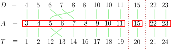
Figure 2: A 2-Visits instance $D$, with its discretized sequence $A$ consisting of three clusters (marked with red). $T$ is the respective set of targets (gaps). Green lines among $D,A,T$ show triplets that constitute solutions to each of the three Position Matching instances obtained through Theorem 2.

Figure 3: The sequence $A$ of Fig. 2 with its gaps and the schedule $S$ found by solving the Position Matching instances. Primary visits are denoted with orange and secondary visits with blue. For simplicity, we use the nodes’ deadlines to show the schedule (instead of their indices).

4.3 2-Visits with distinct deadlines

Let $D=\langle d_{1},\ldots,d_{n}\rangle$ be a sequence containing distinct deadlines. For its discretized sequence $A=\langle a_{1},\ldots,a_{n}\rangle$ it holds that $A=D$, by Definition 5. By Theorem 2, the 2-Visits instance $D$ reduces in linear time to solving a Position Matching instance of the form $I=(D^{\prime}=\langle d_{p},\ldots,d_{q}\rangle,A^{\prime}=\langle a_{p},\ldots,a_{q}\rangle,T)$ for each cluster $A^{\prime}$. Observe that $D^{\prime}=A^{\prime}$, which renders $I$ trivial through the restriction that $d\in D^{\prime}$ cannot be matched with $a\in A^{\prime}$ s.t. $d<a$: $d_{p}$ can only be matched with $a_{p}$ and, thus, $d_{p+1}$ can only be matched with $a_{p+1}$ and so on. The Position Matching instance $I$ has a solution if and only if this unique feasible matching between $D^{\prime}$ and $A^{\prime}$ satisfies every target in $T$, leading to the following lemma.

Lemma 8.

A Position Matching instance $(D,A,T)$ with $D$ containing only distinct numbers can be solved in $\mathcal{O}(n)$ time.

To construct the respective feasible schedule for the 2-Visits instance $D$, we have to place the secondary visits in gaps by increasing induced deadline, according to Theorem 1. However, sorting them by induced deadline in this case is unnecessary, since the aforementioned matching always places the primary visits by increasing deadline, meaning that the nodes are already in the desired order. Thus, we obtain the following theorem.

Theorem 3.

A 2-Visits instance with distinct deadlines can be solved in $\mathcal{O}(n)$ time. A respective schedule (if it exists) can be constructed in $\mathcal{O}(n)$ time as well.

4.4 2-Visits with constant maximum cluster size

Let $D$ be a 2-Visits instance and $A$ its discretized sequence. Let $c$ be the size of the largest cluster of $A$. By Theorem 2, 2-Visits reduces in linear time to solving a Position Matching instance of size $\mathcal{O}(c)$ for each cluster. Since the number of clusters is bounded by $n$, 2-Visits can be solved in $\mathcal{O}(nc!)$ time by running a brute force algorithm for Position Matching.

Corollary 3.

There is an FPT algorithm for 2-Visits parameterized by the maximum cluster size of the input’s discretized sequence.

4.5 2-Visits with up to two distinct numbers

Observation 4.

A Position Matching instance $(D,A,T)$ with $D$ only containing copies of a single number is trivial. It suffices to add that number to each $a\in A$ and check whether all $t\in T$ are satisfied.

Corollary 4.

A 2-Visits instance that only contains copies of a single number can be solved in $\mathcal{O}(n)$ time.

We now discuss the case where $D$ consists of only two distinct deadlines. That is, $D=\langle d_{1},\ldots,d_{n}\rangle$ contains $m$ copies of $x$ and $n-m$ copies of $y>x$. Let $A=\langle a_{1},\ldots,a_{n}\rangle$ be the discretized sequence of $D$. For $i\neq m$ it holds that $a_{i+1}=a_{i}+1$, since $d_{i}=d_{i+1}$. We will show an algorithm for 2-Visits with two distinct deadlines by considering the cases $a_{m+1}\neq a_{m}+1$ and $a_{m+1}=a_{m}+1$ separately.

Lemma 9.

A 2-Visits instance $D=\langle d_{1},\ldots,d_{n}\rangle$ with $d_{1}=d_{2}=\ldots=d_{m}=x$, $d_{m+1}=\ldots=d_{n}=y$, $x<y$, can be solved in $\mathcal{O}(n)$ time if $a_{m+1}\neq a_{m}+1$.

Proof.

Since all $a_{i}\in A$ except $a_{m},a_{m+1}$ are consecutive numbers, $A$ consists of exactly two clusters: $C_{1}=\langle a_{1},\ldots,a_{m}\rangle$ and $C_{2}=\langle a_{m+1},\ldots,a_{n}\rangle$. By Theorem 2, it remains to solve two Position Matching instances, one for the first $m$ elements of $D$ and $A$ and another for the remaining $n-m$ elements of $D$ and $A$. The first Position Matching instance receives as input a set $D^{\prime}$ containing only copies of $x$, rendering it trivial by Observation 4. The same holds for the second Position Matching instance with $y$. ∎

Observation 5.

If for a Position Matching instance $I=(D,A,T)$ there exists some $t\in T$ s.t. $t\leq\min(D)+\min(A)$, then $t$ is satisfied by any feasible pair $(d,a)\in D\times A$. It suffices to match $t$ with $\min(D)$ and $\min(A)$; if there is no solution with this choice, then there is no solution for $I$.

Lemma 10.

A 2-Visits instance $D=\langle d_{1},\ldots,d_{n}\rangle$ with $d_{1}=d_{2}=\ldots=d_{m}=x$, $d_{m+1}=\ldots=d_{n}=y$, $x<y$, can be solved in $\mathcal{O}(n)$ time if $a_{m+1}=a_{m}+1$.

Proof.

All numbers in $A$ are consecutive, therefore $A$ is itself a cluster. By Theorem 2, the 2-Visits instance $D$ is equivalent to the Position Matching instance $I=(D,A,T)$, with $T$ consisting of the first $n$ gaps, i.e., $T=T_{1}\cup T_{2}$, where $T_{1}=\{1,\ldots,a_{1}-1\}$, $T_{2}=\{a_{1}+n,\ldots,2n\}$. Targets in $T_{1}$ are small enough to be satisfied by every pair $(d,a)\in D\times A$, so we can match them with the $a_{1}-1$ smallest elements of $D$ and the $a_{1}-1$ smallest elements of $A$ and remove all of these matched elements from the input, by Observation 5. Let $I^{\prime}=(D^{\prime},A^{\prime},T_{2})$ be the (equivalent) Position Matching instance obtained after this step.

If all copies of $x$ in $D$ were used in the last step, $I^{\prime}$ is trivial by Observation 4. Suppose that at least one copy of $x$ remains in $D^{\prime}$. Let $a=\min(A^{\prime})$, $t=\min(T_{2})$ and check whether $a+x$ satisfies $t$. If it does, then $t$ is satisfied by any pair in $D^{\prime}\times A^{\prime}$ and thus can be matched with $a$ and a copy of $x$ to obtain an equivalent Position Matching instance, by Observation 5. If it does not, then $a$ cannot satisfy any target in $T_{2}$ when matched with a copy of $x$ and, therefore, must be matched with a copy of $y$. If $a+y<t$, then there is no feasible match for $a$, hence $I^{\prime}$ does not have a solution. If $a+y\geq t$, match $a$ and a copy of $y$ with the largest target that they satisfy and remove them from the input.

We can apply the above iteratively for each $a\in A^{\prime}$. In each step, we either match $a$ with some $d\in D^{\prime}$ and some $t\in T_{2}$ or we conclude that $I^{\prime}$ has no solution. Since $a+y$ strictly increases in each iteration, finding the largest target satisfied by $a+y$ takes $\mathcal{O}(n)$ time for all iterations combined, if we keep a pointer in $T_{2}$ for the last such target found previously. The process terminates when all copies of $x$ or all copies of $y$ in $D^{\prime}$ are used up, since the remaining instance is then trivial by Observation 4. This solves $I^{\prime}$ in $\mathcal{O}(n)$ time. ∎

We obtain the following theorem from Lemmas 9, 10 and Corollary 4.

Theorem 4.

A 2-Visits instance that only contains copies of up to two distinct numbers can be solved in $\mathcal{O}(n)$ time.

5 The computational complexity of 2-Visits

We define the following numerical matching problem, to be used as an intermediate step in our reduction. This problem may be of independent interest as a variation of N3DM.

Definition 11 (IN3DM).

Given a multiset of positive integers $A=\{a_{1},\ldots,a_{n}\}$, the set $B=\{1,\ldots,n\}$ and a multiset of positive integers (targets) $T=\{t_{1},\ldots,t_{n}\}$, the Inequality Numerical 3-Dimensional Matching $(\textnormal{{IN3DM}})$ problem asks whether there is a subset $M$ of $A\times B\times T$ s.t. every $a_{i}\in A$, $b\in B$, $t_{i}\in T$ occurs exactly once in $M$ and for every triplet $(a,b,t)\in M$ it holds that $a+b\geq t$.

In this section we present a three-step reduction, from RN3DM [31] to IN3DM  to Position Matching and, finally, to 2-Visits. We consider this our main technical contribution.

Remark 2.

Membership in NP is trivial for most problems considered in this paper and is thus always omitted. The exception is Pinwheel Scheduling (and its generalization in Section 6), for which membership in NP, NP-hardness and PSPACE-completeness are all open questions ever since its introduction in 1989 [24].

5.1 Reducing RN3DM to IN3DM

We will use the following restricted version of N3DM for our reduction, defined by Yu et al. [31]. Its constraints are vital for the reduction to Position Matching in the next subsection.

Definition 12 (RN3DM).

Given a multiset of positive integers $A=\{a_{1},\ldots,a_{n}\}$, sets $B=C=\{1,\ldots,n\}$ and an integer $\sigma$ such that

$$\sum_{i=1}^{n}(a_{i}+2i)=n\sigma,$$

the Restricted Numerical 3-Dimensional Matching $(\textnormal{{RN3DM}})$ problem asks whether there is a subset $M$ of $A\times B\times C$ s.t. every $a_{i}\in A$, $b\in B$, $c\in C$ occurs exactly once in $M$ and for every triplet $(a,b,c)\in M$ it holds that $a+b+c=\sigma$.

Theorem 5 (Yu et al. 2004 [31]).

RN3DM is strongly NP-complete.

Theorem 6.

RN3DM reduces to IN3DM in polynomial time.

Proof.

Let $I=(A,B,C,\sigma)$ be a RN3DM instance. Define the set $T=\{\sigma-i\mid i\in C\}$. By the RN3DM constraints, it holds that

$$\sum_{i=1}^{n}(a_{i}+i)=n\sigma-\sum_{i=1}^{n}i=\sum_{i=1}^{n}t_{i}.$$ (2)

Define the IN3DM instance $I^{\prime}=(A,B,T)$. $I^{\prime}$ is a yes-instance of IN3DM if and only if there is a subset $M$ of $A\times B\times T$ s.t. every $a_{i}\in A$, $b_{i}\in B$, $t_{i}\in T$ occurs exactly once in $M$ and for every triplet $(a,b,t)\in M$ it holds that $a+b\geq t$. By (2), $a+b\geq t$, $\forall(a,b,t)\in M$ is equivalent to $a+b=t$, $\forall(a,b,t)\in M$. Equivalently, there is a subset $M^{\prime}$ of $A\times B\times C$ s.t. every $a_{i}\in A$, $b_{i}\in B$, $c_{i}\in C$ occurs exactly once in $M^{\prime}$ and for every triplet $(a,b,c)\in M^{\prime}$ it holds that $a+b=\sigma-c$. Thus, $I^{\prime}$ is a yes-instance of IN3DM if and only if $I$ is a yes-instance of RN3DM. ∎

Lemma 11.

IN3DM is strongly NP-complete, even when $\max(A)-\min(A)\leq 2n-2$ and $T$ is a set (instead of a multiset).

Proof.

The reduction of Theorem 6 already forces $T$ to be a simple set. It remains to prove that IN3DM is strongly NP-complete, even when $\max(A)-\min(A)\leq 2n-2$.

Let $I=(A,B,C,\sigma)$ be a RN3DM instance, where $B=C=\{1,\ldots,n\}$. In any RN3DM solution, the triplet containing $\max(A)$ cannot have a sum smaller than $\max(A)+2$ and the triplet containing $\min(A)$ cannot have a sum larger than $\min(A)+2n$. For a valid RN3DM solution, all triplets $(a,b,c)\in M$ must have sum equal to $\sigma$ and, thus, any RN3DM instance with $\max(A)-\min(A)>2n-2$ is a trivial no-instance. Hence, we can assume that $\max(A)-\min(A)\leq 2n-2$ for the reduction of Theorem 6.

The reduction of Theorem 6 does not modify $A$, which implies that the respective IN3DM instance will also satisfy $\max(A)-\min(A)\leq 2n-2$. In conjunction with Theorem 5, this proves the lemma. ∎

5.2 Reducing IN3DM to Position Matching

For the following reduction we need to pay attention to the constraints of the Position Matching problem (Def. 10). Specifically, for a Position Matching instance $(D,A,T)$:

• $A$ is the discretized sequence of $D$.

• $T$ only contains distinct positive integers.

• Elements in $D$ cannot be matched with larger elements of $A$.

Lemma 11 will be useful for ensuring that these constraints are satisfied. The main challenge in the reduction of this subsection is to force the second set to be the discretized sequence of the first one, while simultaneously enforcing equivalence between the two instances despite the fact that IN3DM allows elements of the first set to be matched with larger elements. We first prove an auxiliary lemma.

Lemma 12.

Any IN3DM instance $I=(A,B,T)$ satisfying the properties of Lemma 11 can be reduced in polynomial time to an IN3DM instance $I^{\prime}=(A^{\prime},B,T^{\prime})$ such that:

1. $\min(A^{\prime})=n$.

2. $\max(A^{\prime})<3n$.

3. $\max(T^{\prime})<4n$.

4. $T^{\prime}$ contains distinct elements.

Proof.

First, assume that for some IN3DM instance $I=(A,B,T)$, $B=\{1,\ldots,n\}$, there is some $t\in T$ s.t. $t\leq\min(A)$. Then, $t$ can be satisfied by every pair $(a,b)\in A\times B$. We observe that if $I$ has a solution, then it has a solution that matches $\min(A)$ and $\min(B)$ with $t$. Thus, we can remove $\min(A)$, $\min(B)=1$ and $t$ from the input and subtract $1$ from all remaining elements of $B$ and $T$. The new IN3DM instance has a solution if and only if $I$ has a solution. We can apply the aforementioned process repeatedly until $t>\min(A)$, $\forall t\in T$. Note that this process preserves the properties of Lemma 11.

Let $I=(A,B,T)$ be an IN3DM instance, satisfying $t>\min(A)$, $\forall t\in T$, as well as the properties of Lemma 11. Observe that, if $\max(T)>\max(A)+n$, then $\max(T)$ cannot be satisfied by any $(a,b)\in A\times B$, rendering $I$ a trivial no-instance. Hence, for our reduction we can assume that

$$\max(T)\leq\max(A)+n.$$ (3)

We now transform $I$ as follows to obtain an equivalent IN3DM instance $I^{\prime}=(A^{\prime},B,T^{\prime})$, while preserving the properties of Lemma 11.

• If $\min(A)<n$, increase all $a\in A$ and all $t\in T$ by $n-\min(A)$.

• If $\min(A)>n$, decrease all $a\in A$ and all $t\in T$ by $\min(A)-n$. Note that no element in $T$ will become non-positive by this operation, since $t>\min(A)$, $\forall t\in T$.

We obtain sets $A^{\prime},\ T^{\prime}$ with $\min(A^{\prime})=n$ and $\max(A^{\prime})-\min(A^{\prime})\leq 2n-2$, implying $\max(A^{\prime})<3n$. At this point, we have proven the first two desired properties for $I^{\prime}$. For the third property, we use (3) to obtain $\max(T^{\prime})\leq\max(A^{\prime})+n<3n+n=4n$. By construction, $T^{\prime}$ contains distinct elements, thus proving all four desired properties.

We now prove the correctness of the reduction. Since we added (or subtracted) the same value to all $a\in A$ and all $t\in T$, any triplet $(a,b,t)\in A\times B\times T$ that satisfied $a+b\geq t$ will satisfy the respective inequality with the modified elements and vice versa, implying that $I$ and $I^{\prime}$ are equivalent. ∎

Theorem 7.

IN3DM reduces to Position Matching in polynomial time.

Proof.

By Lemmas 11, 12, we may consider an IN3DM instance $I=(A,B,T)$, $B=\{1,\ldots,n\}$, satisfying the four properties of Lemma 12. We construct a Position Matching instance $I^{*}=(A^{*},B^{*},T^{*})$ based on $I$ as follows.

• $A^{*}$ is a non-decreasing sequence consisting of the elements in $A$ and $3n$ copies of $4n$.

• $B^{*}$ is an increasing sequence consisting of the elements in $B$ and elements $n+1,\ldots,4n$.

• $T^{*}$ is a set containing the elements in $T$, along with elements $5n+1,\ldots,8n$.

$A^{*},B^{*},T^{*}$ have size $4n$ each. We call the $3n$ new elements added to each set dummy elements. Observe that all dummy elements are larger than all respective non-dummy elements, by properties $2,3$ of Lemma 12. Note that $T^{*}$ only contains distinct positive integers, by properties $3,4$ of Lemma 12. Hence, in order to prove that $I^{*}$ is a valid Position Matching instance, it suffices to prove that $B^{*}$ is the discretized sequence of $A^{*}$.

$A^{*}$ contains $3n$ copies of $4n$, implying that the $3n$ largest elements of its discretized sequence are $n+1,\ldots,4n$. For all non-dummy elements $a\in A^{*}$ it holds that $n\leq a<3n$, by properties $1,2$ of Lemma 12; hence, we obtain that the discretized sequence of $A^{*}$ is $\langle 1,\ldots,4n\rangle$, which is exactly equal to $B^{*}$. This proves that $I^{*}$ is a valid Position Matching instance. We will now prove that $I^{*}$ has a solution if and only if $I$ has a solution.

For any solution of $I^{*}$, the target $8n$ can only be satisfied by matching one of the dummies in $A^{*}$ (of value $4n$) with the largest dummy in $B^{*}$. Suppose we remove the respective triplet from the input. Inductively, the largest remaining dummy target in $T^{*}$ can only be satisfied by matching a dummy of $A^{*}$ (of value $4n$) with the largest available dummy in $B^{*}$. Thus, for any feasible solution of $I^{*}$, all dummies of $A^{*}$ must be matched with dummies of $B^{*}$, satisfying all dummy targets $t\in T^{*}$.

We infer that $I^{*}$ has a solution if and only if there is a partial solution for its non-dummy elements, i.e., the non-dummy elements $a\in A^{*},b\in B^{*},t\in T^{*}$ can be matched in triplets $(a,b,t)$ s.t. $a\geq b$ and $a+b\geq t$. However, the first of these two inequalities holds for all non-dummy $(a,b)$ pairs, since $a\geq n$ for all non-dummy $a\in A^{*}$ and $b\leq n$ for all non-dummy $b\in B^{*}$. This implies that any solution of $I$ is a feasible partial solution for the non-dummy elements in $I^{*}$ (and vice versa, with the other direction following immediately from the definitions of the two problems). From all the above, we obtain that $I$ has a solution if and only if $I^{*}$ has a solution. The reduction described is polynomial-time, since only $3n$ elements were added to each set. ∎

Corollary 5.

Position Matching is strongly NP-complete, even when the discretized sequence consists of consecutive numbers.

5.3 Reducing Position Matching to 2-Visits

The following observation follows immediately from Def. 10 and is an important tool for the reductions presented below.

Observation 6.

Let $(D,A,T)$ be a Position Matching instance and $c$ be any positive integer. Suppose we increase every $e\in D\cup A$ by $c$ and every $t\in T$ by $2c$, obtaining modified sets $D^{\prime},A^{\prime},T^{\prime}$. Recall that $A$ is the discretized sequence of $D$ (see Def. 10). Observe that $A^{\prime}$ is the discretized sequence of $D^{\prime}$ and thus $(D^{\prime},A^{\prime},T^{\prime})$ is a valid Position Matching instance. $(D^{\prime},A^{\prime},T^{\prime})$ is a yes-instance of Position Matching if and only if $(D,A,T)$ is a yes-instance of Position Matching.

Lemma 13.

Any Position Matching instance $I=(D,A,T)$ can be reduced to a Position Matching instance $I^{\prime}=(D^{\prime},A^{\prime},T^{\prime})$ such that $t>a$, $\forall t\in T^{\prime},a\in A^{\prime}$, in polynomial time.

Proof.

We use Observation 6 to add $a_{n}$ to each $e\in D\cup A$ and $2a_{n}$ to each $t\in T$, obtaining an equivalent Position Matching instance $I^{\prime}=(D^{\prime},A^{\prime},T^{\prime})$. We have $\max(A^{\prime})=2a_{n}<\min(T^{\prime})$, which proves the lemma. ∎

Observation 7.

If Lemma 13 is applied to a Position Matching instance $I=(D,A,T)$ such that $A$ consists of consecutive numbers, then $A^{\prime}$ will also consist of consecutive numbers.

We now present our main theorem, whose proof utilizes results from Section 4.

Theorem 8 (Main Theorem).

Position Matching reduces to 2-Visits in polynomial time.

Proof.

We begin by restricting the Position Matching problem to specific instances.

By Corollary 5, Lemma 13 and Observation 7, we may assume a Position Matching instance $I=(D=\langle d_{1},\ldots,d_{n}\rangle,\ A=\langle a_{1},\ldots,a_{n}\rangle,\ T=\{t_{1},\ldots,t_{n}\})$ such that $A$ is the discretized sequence of $D$ and consists of consecutive numbers and $t>a$, $\forall t\in T,a\in A$. Additionally, $t_{i}\neq t_{j}$, $\forall i\neq j$ $(i,j\in[n])$, by Def. 10. We assume $D,A,T$ are all sorted in non-decreasing order. If $a_{1}$ is even, we use Observation 6 to add $1$ to each $e\in D\cup A$ and $2$ to each $t\in T$, obtaining an equivalent Position Matching instance. From now on, we assume that $a_{1}$ is odd.

By Def. 5, it holds that $d_{n}=a_{n}$, which implies that the largest possible sum (of an element in $D$ and an element in $A$) is $2a_{n}$. If $t_{n}>2a_{n}$, then $I$ is a trivial no-instance, since $t_{n}$ is impossible to satisfy. From now on, we assume that $t_{n}\leq 2a_{n}$.

We will now build an instance $D^{\prime}$ of 2-Visits from an instance $I=(D,A,T)$ of Position Matching with the aforementioned assumptions. We let $D^{\prime}=S||D||L$, where:

• $S$ contains small deadlines $s_{i}=2i-1$, $i\in[(a_{1}-1)/2]$. Note that these are all the odd integers smaller than $a_{1}$.

• $L$ contains large deadlines $l_{i}$, one for each number $l\in[a_{n}+1,2a_{n}]\setminus T$. Since $t_{n}\leq 2a_{n}$, it holds that $T\subseteq[a_{n}+1,2a_{n}]$, so every number in $[a_{n}+1,2a_{n}]$ is either in $L$ or in $T$.

We will prove that $I$ is equivalent to $D^{\prime}$ by proving that all visits of nodes $s_{i}\in S$ and $l_{i}\in L$ can be placed feasibly in a 2-Visits schedule satisfying the properties of Theorem 1, regardless of the placement of the visits of nodes $d_{i}\in D$. For convenience, we will say “nodes $s_{i}$” instead of “nodes with deadlines $s_{i}$” throughout this reduction (same for $d_{i}$, $l_{i}$).

Let $A^{\prime}$ be the discretized sequence of $D^{\prime}$. Observe that all $s_{i}\in S$ and $l_{i}\in L$ are distinct and they are smaller or larger than all $a_{i}\in A$ respectively. Hence, $A^{\prime}$ consists of all $s_{i}\in S$, all $a_{i}\in A$ and all $l_{i}\in L$, by Def. 5. Since all $s_{i}\in S$ are distinct odd numbers smaller than $a_{1}$, each $s_{i}\in S$ forms a cluster by itself and all even-numbered positions up to $a_{1}$ are gaps. By Theorem 1, we know that the 2-Visits instance $D^{\prime}$ has a feasible schedule if and only if it has a feasible schedule $F$ satisfying the properties mentioned in that theorem. By Lemmas 6, 7, we know that the following hold for $F$:

1. The primary visit of node $s_{i}$ is placed in position $s_{i}$, for all $s_{i}\in S$.

2. The secondary visit of node $s_{i}$ is placed in the first available gap, i.e., in position $s_{i}+1$, for all $s_{i}\in S$.

The above satisfies both the deadlines and the induced deadlines of nodes $s_{i}\in S$. Since we have assumed $a_{1},\ldots,a_{n}$ are consecutive numbers, they all belong to the same cluster $C$ of $A^{\prime}$. $C$ also contains all $l_{i}\in L$ s.t. $l_{i}<t_{1}$, by definition. By Theorem 1 and Lemma 6, $F$ must place the primary visits of nodes $d_{i}\in D$ and $l_{i}<t_{1}$ collectively in a permutation of the positions $a_{i}\in A$ and $l_{i}<t_{1}$. However, since $l_{i}>a_{n}=d_{n}$, $\forall l_{i}\in L$, the primary visits of nodes $d_{i}\in D$ cannot be placed in positions $l_{i}<t_{1}$. Thus, primary visits of nodes $d_{i}\in D$ have to be placed in a permutation of the positions $a_{i}\in A$ and primary visits of nodes $l_{i}<t_{1}$ have to be placed in a permutation of the positions $l_{i}<t_{1}$.

We place the primary visit of each node $l_{i}\in L$ in position $l_{i}$. Thus, the induced deadline of the node $l_{1}=\min(L)$ is $2l_{1}>2a_{n}\geq t_{n}$. This implies that the secondary visit of the node $l_{1}$ can be placed in position $2a_{n}+1$ of the schedule; this position is larger than all deadlines in $D^{\prime}$, hence it cannot be occupied by any primary visit. Since $l_{i}\in L$ are distinct by definition, the induced deadline of $l_{i+1}$ is larger than the induced deadline of $l_{i}$ by at least $2$, which implies that the secondary visit of $l_{i+1}$ can be placed directly after the secondary visit of $l_{i}$, for all $i\in[|L|-1]$. Inductively, this process places all secondary visits of nodes $l_{i}\in L$ in feasible positions.

At this point, we have shown that there is a feasible placement of all primary and secondary visits of nodes $s_{i}\in S$ and $l_{i}\in L$, satisfying the properties of $F$ imposed by Theorem 1 and Lemmas 6, 7. $F$ is further required to place the primary visits of nodes $d_{i}\in D$ in a permutation of the positions $a_{i}\in A$ and the respective secondary visits in the first $n$ gaps that have not been used by preceding clusters (i.e., by the secondary visits of nodes $s_{i}\in S$), in order of non-decreasing induced deadline. Observe that these $n$ gaps are still available; they are exactly the $n$ positions $t_{i}\in T\subseteq[a_{n}+1,2a_{n}]$, which have not been used by nodes $l_{i}\in L$. This is because $l_{i}\notin T$ by definition and the primary visits of nodes $l_{i}\in L$ are placed in positions $l_{i}$; also, the secondary visits of $l_{i}\in L$ are placed in positions greater than $2a_{n}$, which are strictly greater than every $t\in T$.

We are now ready to show equivalence between $I$ and $D^{\prime}$. By the above, it is shown that a schedule $F$ with the properties of Theorem 1 exists for $D^{\prime}$ if and only if the primary visits of nodes $d_{i}\in D$ can be placed in a permutation of the positions $a_{i}\in A$, s.t. there is some sufficiently large induced deadline for each gap $t_{i}\in T$ and each $d_{i}$ is placed in a position smaller than or equal to itself. This corresponds exactly to the Position Matching instance $I=(D,A,T)$. By Theorem 1, the existence of $F$ is equivalent to the feasibility of $D^{\prime}$. Thus, $I$ has a solution if and only if $D^{\prime}$ has a feasible schedule, which completes the reduction. ∎

Corollary 6 (Main Result).

2-Visits is strongly NP-complete.

Remark 3.

2-Visits is NP-complete only if multisets are allowed as input. For simple sets, it can be solved in linear time, by Theorem 3.

6 Hardness for generalizations of $k$-Visits and Pinwheel Scheduling

Definition 13 (Var-$k$-Visits).

Given $nk$ positive integers $d_{ij}$, $i\in[n],\ j\in[k]$, the Variable $k$-Visits problem $(\textnormal{{Var-}$k${-Visits}})$ asks whether there exists a schedule of length $nk$, containing each $i\in[n]$ exactly $k$ times, with the constraint that the $j$-th occurrence of $i$ is at most $d_{ij}$ positions away from the previous one (or $d_{i1}$ positions from the beginning of the schedule, if $j=1$).

Intuitively, Var-$k$-Visits is a generalization of $k$-Visits in which the deadline of each node is not constant throughout the schedule, but varies depending on how many times the node has been visited.

Theorem 9.

Var-$k$-Visits is strongly NP-complete for all $k\geq 2$, even when $d_{i1}=d_{i2}$ and $d_{ij}=d_{ij^{\prime}}$, $\forall j\in[3,k],j^{\prime}\in[3,k]$, for all nodes $i\in[n]$.

Proof.

We will reduce 2-Visits to Var-$k$-Visits ($k\geq 2$). Let $D=\langle d_{1},\ldots,d_{n}\rangle$ be a 2-Visits instance. We will build a Var-$k$-Visits instance $G$ with deadlines $g_{ij}$, $i\in[n]$, $j\in[k]$. We define:

$$g_{ij}=\begin{cases}d_{i},\ j\leq 2\\ 3n,\ j>2\end{cases}$$

If there is a feasible schedule for $D$, then we can extend it by visiting all nodes $1,\ldots,n$ in this order $k-2$ times in a row, after its end. Since $g_{ij}=3n$ for $j>2$, the modified schedule is feasible for $G$.

Suppose there is a feasible schedule $F$ for $G$. We will create another schedule $F^{\prime}$ based on $F$ in the following manner, and prove that it is feasible for $D$. Scan $F$ from start to end. When a first or second visit of any node is encountered, add a visit of that node to $F^{\prime}$ in its earliest unoccupied position. Thus, the $2n$ positions of $F^{\prime}$ contain exactly two visits of each node, in the same order in which they were encountered in $F$. The following properties hold for every $i\in[n]$:

• The first visit of $i$ in $F^{\prime}$ occurs no later than in $F$.

• The second visit of $i$ in $F^{\prime}$ is at least as close to its respective first visit as it was in $F$.

Hence, all first and second visits have been placed feasibly in $F^{\prime}$, which implies that $F^{\prime}$ is a feasible schedule for $D$.

We infer that $D$ has a feasible schedule if and only if $G$ has a feasible schedule, which completes the reduction. ∎

Similarly, we define a generalization of Pinwheel Scheduling in which the deadline of each node changes after a given threshold of visits.

Definition 14 (Threshold Pinwheel Scheduling).

Given $2n$ positive integers (deadlines) $d_{ij}$, $i\in[n],\ j\in\{1,2\}$, and $n$ positive integers (thresholds) $t_{i}$, $i\in[n]$, the Threshold Pinwheel Scheduling problem asks whether there exists an infinite schedule $p_{1},p_{2},\ldots$ , where $p_{j}\in[n]$ for $j\in\mathbb{N}$, such that for all $i\in[n]$:

• Up until the $t_{i}$-th occurrence of $i$, any $d_{i1}$ consecutive entries contain at least one occurrence of $i$.

• After the $t_{i}$-th occurrence of $i$, any $d_{i2}$ consecutive entries contain at least one occurrence of $i$.

Theorem 10.

Threshold Pinwheel Scheduling is strongly NP-hard (even with explicit input).

The proof of Theorem 10 is almost identical to that of Theorem 9 (by setting $t_{i}=2,\ \forall i\in[n]$, and reducing from 2-Visits) and is thus omitted. The strong NP-hardness result carries over to an even more general version of Pinwheel Scheduling, in which each node changes its deadline a finite amount of times (instead of just once).

7 Conclusion

Our work highlights that finite versions of Pinwheel Scheduling are strongly NP-complete, also implying strong NP-hardness for a natural generalization of the infinite version, which we call Threshold Pinwheel Scheduling. Thus, we show that Pinwheel Scheduling becomes strongly NP-hard when the deadline of each task is allowed to change once during the schedule, which may provide insight towards settling the long-standing open questions concerning the time complexity of the problem.

Our findings lead to several interesting directions for future work. One such direction is to explore special cases in which 2-Visits is tractable. We believe there may exist an FPT algorithm parameterized by the number of numbers, which is a common parameterization for numerical matching problems [18]; we already showed that the problem is tractable when there are only up to two distinct numbers. Also, since 2-Visits is in P for distinct deadlines, there may exist an FPT algorithm parameterized by the maximum multiplicity of the input elements. Another natural direction for future research is to study the complexity of the $k$-Visits problem for $k>2$. We conjecture that $3$-Visits is strongly NP-complete even for distinct deadlines.

The $k$-Visits problem that we studied here can be modeled by an agent traversing a complete graph with deadlines. Equivalently, the problem can be modeled by a star graph where the center is a special node with no deadline. Hence, a natural direction for future work is to study the $k$-Visits problem in other graph classes, e.g. lines or comb graphs. This could help identify additional tractable instances for deadline-based problems.

Our results and the open questions arising from this work may contribute to the ongoing effort to understand the complexity of Pinwheel Scheduling. It still remains open whether Pinwheel Scheduling is NP-hard (for explicit input), whether it is contained in NP, and whether it is PSPACE-complete. By analyzing $k$-Visits and Threshold Pinwheel Scheduling, we provide new insights that could help address these questions.

Acknowledgements

This work has been partially supported by project MIS 5154714 of the National Recovery and Resilience Plan Greece 2.0 funded by the European Union under the NextGenerationEU Program.

References

- [1] Baller, A.C., van Ee, M., Hoogeboom, M., Stougie, L.: Complexity of inventory routing problems when routing is easy. Networks 75(2), 113–123 (2020). https://doi.org/10.1002/NET.21908, https://doi.org/10.1002/net.21908
- [2] Bar-Noy, A., Dreizin, V., Patt-Shamir, B.: Efficient algorithms for periodic scheduling. Comput. Networks 45(2), 155–173 (2004). https://doi.org/10.1016/J.COMNET.2003.12.017, https://doi.org/10.1016/j.comnet.2003.12.017
- [3] Bar-Noy, A., Ladner, R.E., Christensen, J., Tamir, T.: A general buffer scheme for the windows scheduling problem. ACM J. Exp. Algorithmics 13 (2008). https://doi.org/10.1145/1412228.1412234, https://doi.org/10.1145/1412228.1412234
- [4] Bar-Noy, A., Ladner, R.E., Tamir, T.: Windows scheduling as a restricted version of bin packing. ACM Trans. Algorithms 3(3), 28 (2007). https://doi.org/10.1145/1273340.1273344, https://doi.org/10.1145/1273340.1273344
- [5] Biktairov, Y., Gasieniec, L., Jiamjitrak, W.P., Namrata, Smith, B., Wild, S.: Simple approximation algorithms for polyamorous scheduling. In: Bercea, I.O., Pagh, R. (eds.) 2025 Symposium on Simplicity in Algorithms, SOSA 2025, New Orleans, LA, USA, January 13-15, 2025. pp. 290–314. SIAM (2025). https://doi.org/10.1137/1.9781611978315.23, https://doi.org/10.1137/1.9781611978315.23
- [6] Blin, L., Milani, A., Potop-Butucaru, M., Tixeuil, S.: Exclusive perpetual ring exploration without chirality. In: Distributed Computing, 24th International Symposium, DISC 2010, Cambridge, MA, USA, September 13-15, 2010. Proceedings. pp. 312–327 (2010). https://doi.org/10.1007/978-3-642-15763-9_29, https://doi.org/10.1007/978-3-642-15763-9_29
- [7] Bosman, T., van Ee, M., Jiao, Y., Marchetti-Spaccamela, A., Ravi, R., Stougie, L.: Approximation algorithms for replenishment problems with fixed turnover times. Algorithmica 84(9), 2597–2621 (2022). https://doi.org/10.1007/S00453-022-00974-4, https://doi.org/10.1007/s00453-022-00974-4
- [8] Chan, M.Y., Chin, F.Y.L.: General schedulers for the pinwheel problem based on double-integer reduction. IEEE Trans. Computers 41(6), 755–768 (1992). https://doi.org/10.1109/12.144627, https://doi.org/10.1109/12.144627
- [9] Chan, M.Y., Chin, F.Y.L.: Schedulers for larger classes of pinwheel instances. Algorithmica 9(5), 425–462 (1993). https://doi.org/10.1007/BF01187034, https://doi.org/10.1007/BF01187034
- [10] Chuangpishit, H., Czyzowicz, J., Gasieniec, L., Georgiou, K., Jurdzinski, T., Kranakis, E.: Patrolling a path connecting a set of points with unbalanced frequencies of visits. In: SOFSEM 2018: Theory and Practice of Computer Science - 44th International Conference on Current Trends in Theory and Practice of Computer Science, Krems, Austria, January 29 - February 2, 2018, Proceedings. pp. 367–380 (2018). https://doi.org/10.1007/978-3-319-73117-9_26, https://doi.org/10.1007/978-3-319-73117-9_26
- [11] Czyzowicz, J., Georgiou, K., Kranakis, E.: Patrolling. In: Flocchini, P., Prencipe, G., Santoro, N. (eds.) Distributed Computing by Mobile Entities, Current Research in Moving and Computing, Lecture Notes in Computer Science, vol. 11340, pp. 371–400. Springer (2019). https://doi.org/10.1007/978-3-030-11072-7_15, https://doi.org/10.1007/978-3-030-11072-7_15
- [12] Czyzowicz, J., Godon, M., Kranakis, E., Labourel, A., Markou, E.: Exploring graphs with time constraints by unreliable collections of mobile robots. In: SOFSEM 2018: Theory and Practice of Computer Science - 44th International Conference on Current Trends in Theory and Practice of Computer Science, Krems, Austria, January 29 - February 2, 2018, Proceedings. pp. 381–395 (2018). https://doi.org/10.1007/978-3-319-73117-9_27, https://doi.org/10.1007/978-3-319-73117-9_27
- [13] Damaschke, P.: Two robots patrolling on a line: Integer version and approximability. In: Combinatorial Algorithms - 31st International Workshop, IWOCA 2020, Bordeaux, France, June 8-10, 2020, Proceedings. pp. 211–223 (2020). https://doi.org/10.1007/978-3-030-48966-3_16, https://doi.org/10.1007/978-3-030-48966-3_16
- [14] Das, S.: Graph explorations with mobile agents. In: Distributed Computing by Mobile Entities, Current Research in Moving and Computing, pp. 403–422. Springer (2019). https://doi.org/10.1007/978-3-030-11072-7_16, https://doi.org/10.1007/978-3-030-11072-7_16
- [15] D’Emidio, M., Stefano, G.D., Navarra, A.: Bamboo garden trimming problem: Priority schedulings. Algorithms 12(4), 74 (2019). https://doi.org/10.3390/A12040074, https://doi.org/10.3390/a12040074
- [16] van Ee, M.: A 12/7-approximation algorithm for the discrete bamboo garden trimming problem. Oper. Res. Lett. 49(5), 645–649 (2021). https://doi.org/10.1016/J.ORL.2021.07.001, https://doi.org/10.1016/j.orl.2021.07.001
- [17] Feinberg, E.A., Curry, M.T.: Generalized pinwheel problem. Math. Methods Oper. Res. 62(1), 99–122 (2005). https://doi.org/10.1007/S00186-005-0443-4, https://doi.org/10.1007/s00186-005-0443-4
- [18] Fellows, M.R., Gaspers, S., Rosamond, F.A.: Parameterizing by the number of numbers. Theory Comput. Syst. 50(4), 675–693 (2012). https://doi.org/10.1007/S00224-011-9367-Y, https://doi.org/10.1007/s00224-011-9367-y
- [19] Fishburn, P.C., Lagarias, J.C.: Pinwheel scheduling: Achievable densities. Algorithmica 34(1), 14–38 (2002). https://doi.org/10.1007/S00453-002-0938-9, https://doi.org/10.1007/s00453-002-0938-9
- [20] Garey, M.R., Johnson, D.S.: Computers and Intractability: A Guide to the Theory of NP-Completeness. W. H. Freeman (1979)
- [21] Gasieniec, L., Klasing, R., Levcopoulos, C., Lingas, A., Min, J., Radzik, T.: Bamboo garden trimming problem (perpetual maintenance of machines with different attendance urgency factors). In: Steffen, B., Baier, C., van den Brand, M., Eder, J., Hinchey, M., Margaria, T. (eds.) SOFSEM 2017: Theory and Practice of Computer Science - 43rd International Conference on Current Trends in Theory and Practice of Computer Science, Limerick, Ireland, January 16-20, 2017, Proceedings. Lecture Notes in Computer Science, vol. 10139, pp. 229–240. Springer (2017). https://doi.org/10.1007/978-3-319-51963-0_18, https://doi.org/10.1007/978-3-319-51963-0_18
- [22] Gasieniec, L., Smith, B., Wild, S.: Towards the 5/6-density conjecture of pinwheel scheduling. In: Phillips, C.A., Speckmann, B. (eds.) Proceedings of the Symposium on Algorithm Engineering and Experiments, ALENEX 2022, Alexandria, VA, USA, January 9-10, 2022. pp. 91–103. SIAM (2022). https://doi.org/10.1137/1.9781611977042.8, https://doi.org/10.1137/1.9781611977042.8
- [23] Höhne, F., van Stee, R.: A 10/7-approximation for discrete bamboo garden trimming and continuous trimming on star graphs. In: Megow, N., Smith, A.D. (eds.) Approximation, Randomization, and Combinatorial Optimization. Algorithms and Techniques, APPROX/RANDOM 2023, September 11-13, 2023, Atlanta, Georgia, USA. LIPIcs, vol. 275, pp. 16:1–16:19. Schloss Dagstuhl - Leibniz-Zentrum für Informatik (2023). https://doi.org/10.4230/LIPICS.APPROX/RANDOM.2023.16, https://doi.org/10.4230/LIPIcs.APPROX/RANDOM.2023.16
- [24] Holte, R., Mok, A., Rosier, L., Tulchinsky, I., Varvel, D.: The pinwheel: a real-time scheduling problem. In: [1989] Proceedings of the Twenty-Second Annual Hawaii International Conference on System Sciences. Volume II: Software Track. vol. 2, pp. 693–702 vol.2 (1989). https://doi.org/10.1109/HICSS.1989.48075
- [25] Holte, R., Rosier, L.E., Tulchinsky, I., Varvel, D.A.: Pinwheel scheduling with two distinct numbers. Theor. Comput. Sci. 100(1), 105–135 (1992). https://doi.org/10.1016/0304-3975(92)90365-M, https://doi.org/10.1016/0304-3975(92)90365-M
- [26] Jacobs, T., Longo, S.: A new perspective on the windows scheduling problem. CoRR abs/1410.7237 (2014), http://arxiv.org/abs/1410.7237
- [27] Kawamura, A.: Proof of the density threshold conjecture for pinwheel scheduling. In: Mohar, B., Shinkar, I., O’Donnell, R. (eds.) Proceedings of the 56th Annual ACM Symposium on Theory of Computing, STOC 2024, Vancouver, BC, Canada, June 24-28, 2024. pp. 1816–1819. ACM (2024). https://doi.org/10.1145/3618260.3649757, https://doi.org/10.1145/3618260.3649757
- [28] Kawamura, A., Kobayashi, Y., Kusano, Y.: Pinwheel covering. In: Finocchi, I., Georgiadis, L. (eds.) Algorithms and Complexity - 14th International Conference, CIAC 2025, Rome, Italy, June 10-12, 2025, Proceedings, Part II. Lecture Notes in Computer Science, vol. 15680, pp. 185–199. Springer (2025). https://doi.org/10.1007/978-3-031-92935-9_12, https://doi.org/10.1007/978-3-031-92935-9_12
- [29] Lin, S., Lin, K.: A pinwheel scheduler for three distinct numbers with a tight schedulability bound. Algorithmica 19(4), 411–426 (1997). https://doi.org/10.1007/PL00009181, https://doi.org/10.1007/PL00009181
- [30] Shannon, C.E.: Presentation of a Maze Solving Machine, pp. 681–687. IEEE Press (1993). https://doi.org/10.1109/9780470544242.ch44
- [31] Yu, W., Hoogeveen, H., Lenstra, J.K.: Minimizing makespan in a two-machine flow shop with delays and unit-time operations is np-hard. J. Sched. 7(5), 333–348 (2004). https://doi.org/10.1023/B:JOSH.0000036858.59787.C2, https://doi.org/10.1023/B:JOSH.0000036858.59787.c2