Dynamics Simulation of Arbitrary Non-Hermitian Systems Based on Quantum Monte Carlo

Abstract

Non-Hermitian quantum systems exhibit unique properties and hold significant promise for diverse applications, yet their dynamical simulation poses a particular challenge due to intrinsic openness and non-unitary evolution. Here, we introduce a hybrid classical-quantum algorithm based on Quantum Monte Carlo (QMC) for simulating the dynamics of arbitrary time-dependent non-Hermitian systems. Notably, this approach constitutes a natural extension of the quantum imaginary-time evolution (QITE) algorithm. This algorithm combines the advantages of both classical and quantum computation and exhibits good applicability and adaptability, making it promising for simulating arbitrary non-Hermitian systems such as PT-symmetric systems, non-physical processes, and open quantum systems. To validate the algorithm, we applied it to the dynamic simulation of open quantum systems and achieved the desired results.

Introduction.—

The latest advances in quantum physics reveal that non-Hermitian systems exhibit unique physical phenomena not found in traditional Hermitian systems [1, 2, 3, 4], such as parity-time (PT)-symmetry [5, 6, 7], exceptional points [8, 9], and non-Hermitian skin effects [10, 11, 12, 13]. These features not only challenge our fundamental understanding of quantum mechanics but also pave the way for new applications in topological photonics [14, 15, 16, 17], dissipative quantum computation [18, 19] and quantum sensor technologies [20, 21, 22]. However, studies on non-Hermitian systems have once encountered several ”paradoxes”, which seemed to conflict with traditional quantum mechanics or relativity theories, such as the instantaneous quantum brachistochrone problem [23, 24], deterministic successful discrimination of non-orthogonal quantum states [25, 26], and violation of the no-signaling principle [27, 28]. Nevertheless, it was later discovered that these paradoxes stemmed from our ignorance of how to simulate PT-symmetric systems within traditional quantum systems, if we account for the probability loss events in the simulation process, the paradoxes are automatically resolved [29].

However, many quantum many-body problems are intractable in classical simulation and classical computation. One obvious reason is that the dimension of Hilbert space grows exponentially with the system size, making it impossible to store the wave function of a large system in classical memory. In 1982, Richard Feynman proposed a solution: quantum computation [30, 31], and then Seth Lloyd first proposed a formula for quantum simulation in 1996 [32]. Quantum Monte Carlo (QMC) method, as an important classical algorithm, has been widely applied in fields such as quantum physics , quantum chemistry, and materials science in recent years [33, 34, 35, 36]. The advantages of QMC include its high flexibility and versatility [37, 38] , its ability to efficiently handle quantum many-body problems [39], as well as its feasibility on noisy quantum devices [40, 41]. By combining classical computation with quantum computation, running classical sampling algorithms on classical computers and delegating quantum programs related to the samples to quantum computers, we can construct hybrid classical-quantum algorithms. These algorithms combine the advantages of both classical and quantum computation, offering benefits such as further reducing the depth of quantum circuits [41, 42], mitigating the impact of coherent noise in quantum circuits [43, 44, 45], and alleviating the ”sign problem” [46, 43].

Many non-unitary processes described by superoperators can be transformed into non-Hermitian systems [9, 47, 48]. However, within the traditional framework of quantum mechanics, the evolution of non-Hermitian systems is non-unitary and cannot be directly simulated on quantum computers, and it must be decomposed into unitary operators. Moreover, due to their non-unitary evolution characteristics, non-Hermitian systems do not conserve probability, and their simulation methods are typically accompanied by widespread probability loss events, including all methods that involve post-selection processes, such as the linear combination of unitaries (LCU) method [49, 50], and dilation-based methods [29, 51, 52]. To overcome these drawback, complex probability amplification procedures (such as the oblivious amplitude amplification (OAA) procedure) are usually required [53, 54], which increase the circuit depth, elevate the cost of fault-tolerant quantum computation, and hinder the realization of quantum simulations with practical quantum advantages in the NISQ era. Fortunately, hybrid classical-quantum computation based on QMC can directly avoid these disadvantages [43, 44, 45].

Utilizing the unique properties of non-Hermitian quantum systems, many significant and meaningful tasks can be addressed [55, 56, 21, 41, 42]. Taking quantum imaginary-time evolution as an example [41, 42], it holds great value in solving ground state energies, studying quantum phase transitions and critical phenomena, and combinatorial optimization and quantum machine learning. However, it requires assuming that time is purely imaginary or, equivalently, that the Hamiltonian is an anti-Hermitian Hamiltonian. Furthermore, many problems, such as PT-symmetric systems, open quantum systems, some non-physical processes (non-completely positive trace-preserving map, i.e., non-CPTP maps) [48], and linear algebra problems, may involve non-Hermitian Hamiltonians that are not necessarily anti-Hermitian. Therefore, the Hamiltonian simulation techniques for traditional closed quantum systems, which follow unitary evolution, cannot be directly applied to them.

In this work, we propose a general framework for the dynamic simulation of arbitrary non-Hermitian systems based on QMC, which belongs to hybrid classical-quantum algorithms. Our algorithm can also be regarded as a natural extension of the quantum imaginary-time evolution (QITE) algorithm [41, 42, 47]. When simulating non-Hermitian quantum systems, this framework can avoid the post-selection events that are inevitable in deterministic quantum algorithms based on LCU, which often lead to probability loss and resource waste. Our algorithm is highly versatile and theoretically capable of simulating arbitrary time-dependent non-Hermitian system without assuming that Hamiltonian is anti-Hermitian or diagonalizable, thus holding promise for solving previously challenging problems, such as the simulation of PT-symmetric systems, especially PT-symmetry broken systems (Hamiltonian can not be diagonalizable), and open quantum systems. To verify the feasibility of our scheme, we will present specific applications of this algorithm in the simulation of open quantum systems. Additionally, within this framework, techniques used in Hamiltonian simulation of traditional Hermitian systems, such as quantum error mitigation, can be naturally integrated as subroutines.

Preliminaries.—

In this section, we review the theory of the linear combination of Hamiltonian simulation for non-unitary dynamics (LCHS) [57], which is proposed by Dong An et al in 2023 and latter an optimized version was proposed by them again [58]. This method originated from solving linear differential equation problems, and has been proved to be applicable to quantum simulation. We briefly introduce the scheme as follows.

Given a time-dependent non-Hermitian Hamiltonian $H(t)$, which can always be decomposed into

$$H(t)=H_{r}(t)-iH_{i}(t),$$ (1)

where $H_{r}(t)=[H(t)+H^{\dagger}(t)]/2$, $H_{i}(t)=i[H(t)-H^{\dagger}(t)]/2$. For the non-Hermitian system evolution $\mathcal{T}e^{-i\int_{0}^{t}H(s)ds}$, Dong An et al. have proved that there is a equation when $H_{i}(t)\geqslant 0$,

$$u(t)\equiv\mathcal{T}e^{-i\int_{0}^{t}H(s)ds} =\int_{\mathbb{R}}\frac{f(k)}{1-ik}\mathcal{T}e^{-i\int_{0}^{t}[H_{r}(s)+k\cdot H_{i}(s)]ds}dk$$

$$=\int_{\mathbb{R}}g(k)U(t,k)dk,$$ (2)

where $\mathcal{T}$ is the time-ordering operator, and $f(k)$ is called by them the kernel function, the integrand function $g(k)\equiv\frac{f(k)}{1-ik}$ is the unnormalized complex probability density function related to the continuous random variable $k$, and its normalized probability density function $\mathrm{Pd}(k)=|g(k)|/\|g(k)\|_{1}$, where $\|g\|_{1}\equiv\int_{-\infty}^{\infty}|g(k)|\mathrm{d}k$ is a constant, $e^{i\theta(k)}=g(k)/\|g\|_{1}$ is the phase part. $U(t,k)\equiv\mathcal{T}e^{-i\int_{0}^{t}K_{s}(k)ds}$ is an unitary operator related to the parameter $k$ and time $t$, where $K_{s}(k)\equiv H_{r}(s)+k\cdot H_{i}(s)$ is Hermitian. However, many Hamiltonian systems do not satisfy the conditions $H_{i}(t)\geqslant 0$. In this case, a technical treatment can be applied to the above equation. That is, an additional compensation constant $c_{p}$ is added to $H_{i}(t)$ such that $H_{i}(t)+c_{p}\geqslant 0$. At the same time, the cost is that an additional constant $e^{c_{p}t}$ needs to be multiplied at the end of the right hand side of the above Eq.(Preliminaries.—). More details regarding the kernel function $f(k)$ can be found in Appendix A.

Dynamics simulation of arbitrary non-Hermitian systems based on QMC.—

Many process described by superoperators can be transformed into non-Hermitian systems, such as certain physical processes like the dynamics simulation of open quantum systems [9, 47], as well as some non-physical processes, like non-completely positive actions [48]. Some important algorithms, such as the imaginary-time evolution algorithm, describe non-Hermitian dynamical processes. However, unlike imaginary-time evolution, we do not merely assume that the Hamiltonian is Hermitian and the time is imaginary; instead, the time is real, but the Hamiltonian can be arbitrarily non-Hermitian. We try to use the framework given in the above sections to construct our algorithm. Unlike typical quantum state preparation algorithms, which typically require outputting the correct quantum state itself, the objective of Quantum Monte Carlo algorithms is to output the correct mean value of the given observable $O=\sum_{n}o_{n}O_{n}$, where $o_{n}\in\mathbb{Z}$, $O_{n}$ can be selected as any unitary operator for implementation on quantum circuits, and usually $O_{n}\equiv\sigma_{n}\in\{I,X,Y,Z\}^{\otimes m}$ is general Pauli operator. We assume by default that $O$ can be time-dependent.

Unlike quantum state preparation tasks, quantum simulation based on Quantum Monte Carlo typically focuses on estimating the expectation value $\langle O\rangle(t)\equiv\langle\psi|u^{\dagger}(t)\cdot O\cdot u(t)|\psi\rangle/\|u(t)|\psi\rangle\|^{2}$ of an observable $O$ to a certain precision, rather than on obtaining the final state $u(t)|\psi\rangle/\|u(t)|\psi\rangle\|$. The factor $\|u(t)|\psi\rangle\|$ represents a normalization factor caused by the non-unitary evolution $u(t)$ in the non-Hermitian system. Therefore, the following theorem guarantees the successful implementation of the above quantum simulation task.

Theorem 1.

Given an initial state $|\psi\rangle$, the arbitrary finite-dimensional time-dependent non-Hermitian Hamiltonian $H(t)$, a new Hamiltonian $\tilde{H}(s)=H_{r}(s)-i(H_{i}(s)-{E_{i}}_{0}(s))$ with a manually chosen time-dependent quantity ${E_{i}}_{0}(s)$, the observable $O=\sum_{n}o_{n}O_{n}$, then the estimation $\langle O\rangle(t)$ of the observable $O$ can be synthesized through unbiased estimation of the numerator part $N(O)\equiv\langle\psi|\mathcal{\overline{T}}e^{-i\int_{0}^{T}\tilde{H}^{\dagger}(s)ds}\cdot O\cdot\mathcal{T}e^{-i\int_{0}^{T}\tilde{H}(s)ds}|\psi\rangle$ and the denominator part $D$ (equivalently denoted as $N(I)$) separately,

$$\langle O\rangle=\frac{N(O)}{D}=\frac{\|O\|_{l_{1}}\cdot\mathbb{E}_{k^{\prime},k,n}\langle O_{n}(k^{\prime},k)\cdot e^{i\theta(n)}\cdot e^{i\theta(k^{\prime},k)})\rangle}{\mathbb{E}_{k^{\prime},k}\langle I(k^{\prime},k)\cdot e^{i\theta(k^{\prime},k)}\rangle}.$$ (3)

Here $\langle[\cdot](k^{\prime},k)\rangle\equiv$ $\langle\psi|\mathcal{\overline{T}}e^{i\int_{0}^{T}K_{s^{\prime}}(k^{\prime})ds^{\prime}}[\cdot]\mathcal{T}e^{-i\int_{0}^{T}K_{s}(k)ds}|\psi\rangle$, $\mathcal{\overline{T}}$ is the anti-time-ordering operator, $K_{s}(k)=H_{r}(s)-k\cdot(H_{i}(s)-{E_{i}}_{0}(s))$, where the compensation constant ${E_{i}}_{0}(s)$ can be chosen as any real value to ensure that $H_{i}(s)-{E_{i}}_{0}(s)\geqslant 0$. $\mathbb{E}_{k^{\prime},k,...}\equiv\mathbb{E}_{k^{\prime}}\mathbb{E}_{k},...\mathbb{E}_{[\cdot]}$ represents the expectation with respect to random variables $k$, $k^{\prime}$, $...$, the probability density related to $k$ is $\mathrm{Pd}(k)$, $e^{i\theta(k^{\prime},k)}=e^{i(\theta(k)-\theta(k^{\prime}))}=g^{*}(k^{\prime})g(k)/\|g\|_{1}^{2}$ is the phase part, and the sampling probability of $O_{n}$ is $p_{n}=|o_{n}|/\|O\|_{l_{1}}$, where $\|O\|_{l_{1}}\equiv\sum_{n}|o_{n}|$, $e^{i\theta(n)}\equiv o_{n}/|o_{n}|$ denotes the phase part. Noting that $\|O\|_{l_{1}}\cdot\mathbb{E}_{k^{\prime},k,n}\langle O_{n}(k^{\prime},k)\cdot e^{i\theta(n)}\cdot e^{i\theta(k^{\prime},k)})\rangle=\mathbb{E}_{k^{\prime},k}\langle O(k^{\prime},k)\cdot e^{i\theta(k^{\prime},k)})\rangle$.

Proof.

The proof of this theorem will be provided in Appendix B. ∎

Error and complexity analysis.—

The algorithm will estimate the numerator (the part of $O_{n}(k^{\prime},k)$) and denominator (the part of $I(k^{\prime},k)$) of Eq.(3) respectively. There are two types of errors here in this algorithm, one is systematic error, and the other is statistical error. The systematic error is mainly caused by the limited resolution of quantum gates since the gate angles are defined and implemented using digital electronics [59, 44], and truncation errors since the domain of the integrand function $g(k)$ is $(-\infty,\infty)$ and thus it has to be truncated within a finite interval [42]. The statistical error has two contributing factors, the fluctuation error caused by limited samplings, and the shots noise caused by limited measurements.

Theorem 2.

Given that $\eta$ is the permissible error synthesized by the numerator part and the denominator part, $\delta$ is the statistical failure probability bound, and $\varepsilon$ is the given truncation error, denoting that $\hat{N}(O)=\|g\|_{1}^{2}\cdot\langle O(k^{\prime},k)\cdot e^{i\theta(k^{\prime},k)}\rangle,\overline{\hat{N}}(O)=\frac{1}{n_{N}}\sum_{i=1}^{n_{N}}\hat{N}(O)$, then the inequality

$$\left|\frac{\overline{\hat{N}}(O)}{\overline{\hat{D}}}-\langle O\rangle\right|\leqslant\eta$$ (4)

hold with a probability higher than $1-\delta$. When Hamiltonian $\tilde{H}$ is time-dependent, the algorithm can be effectively implemented with a duration of $T=\mathcal{O}(1/\Delta_{E_{i}})$, $\Delta_{E_{i}}$ represents the maximum bandwidth of $\tilde{H}_{i}(t)=H_{i}(s)-{E_{i}}_{0}(s)$. The query complexity required to the above inequality is $k_{c}=\mathcal{O}\left(T\max_{t}\|\tilde{H}(t)\|\left(\log\left(\frac{1}{\varepsilon}\right)\right)^{1+1/\beta}\right)$, the maximum sampling complexity is $n_{N}=n_{D}=\mathcal{O}\left(\frac{\log(\frac{1}{\delta})\cdot(\|O\|_{l_{1}}+1)^{2}\|g\|_{1}^{4}}{\eta^{2}}\right)$. When $\tilde{H}$ is time-independent, there is no restriction on the duration of the algorithm, and the query complexity required is $k_{c}=\mathcal{O}\left(\left(\log\left(\frac{1}{\varepsilon}\right)\right)^{1/\beta}\right)$, the maximum sampling complexity is $n_{N}=n_{D}=\mathcal{O}\left(\frac{\log(\frac{1}{\delta})\cdot(\|O\|_{l_{1}}+1)^{2}\|g\|_{1}^{4}}{\eta^{2}p_{g}^{2}}\right)$, where $p_{g}\equiv|\langle\phi_{g}|\psi\rangle|^{2}$ is the non-zero overlap between the ground state $|\phi_{g}\rangle$ of $\tilde{H}_{i}$ and the initial state $|\psi\rangle$.

Proof.

The proof of this theorem will be provided in Appendix C. ∎

Finally, by embedding any known Hamiltonian simulation subroutine, the final simulation can be achieved in Appendix D. For reference, we recall a continuous method [44], which also belongs to a class of quantum Monte Carlo methods. It is particularly worth noting that in this subroutine, all errors are independent of the trotter step, so the limited resolution of quantum gates can be inherently resolved. Both systematic and statistical errors can be simultaneously reduced simply by increasing the number of samples. Moreover, this subroutine has been shown to be compatible with time-dependent Hamiltonians as well as non-sparse Hamiltonians, and is particularly well-suited for present-day relatively noisy quantum hardware.

Circuits and Algorithms.—

The circuit of our algorithm is shown in Fig.1, and the process of our algorithm for estimating the numerator $N(O)$ and the denominator $D$ are shown in Algorithm 1. Their measurements are carried out separately for the real and imaginary parts, as detailed in Appendix E.

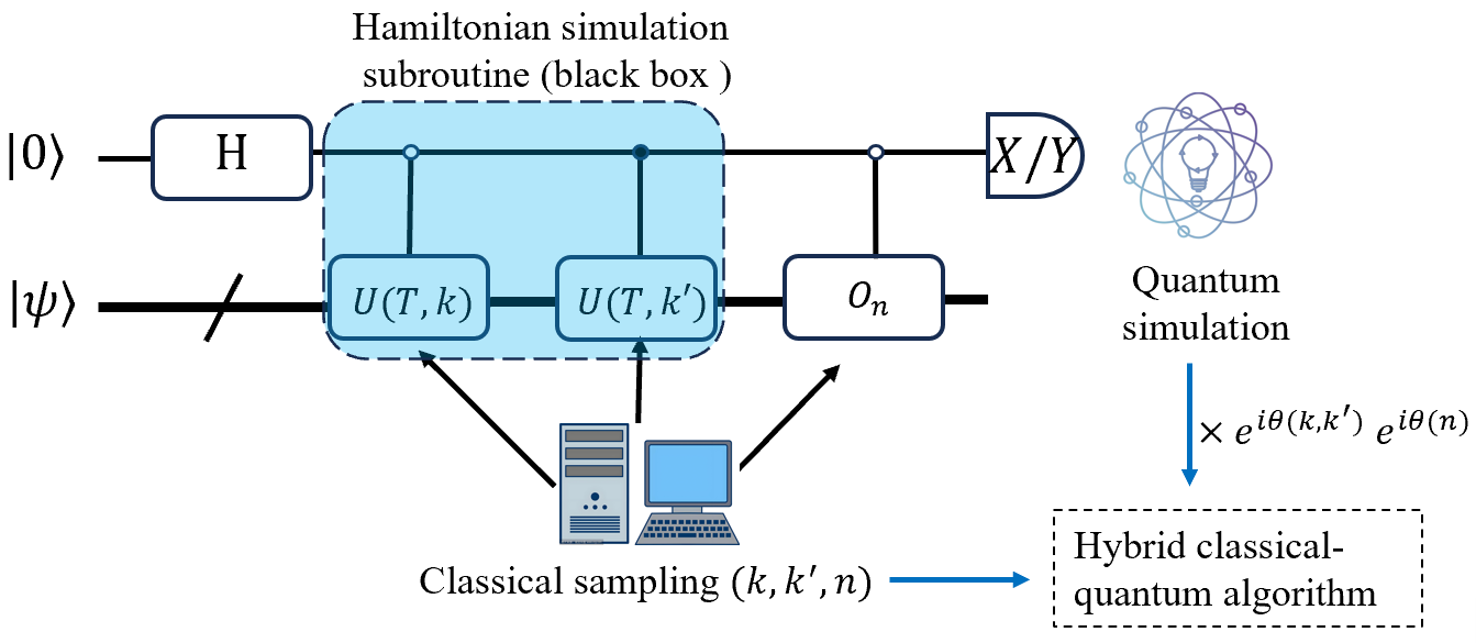
Figure 1: Hybrid classical-quantum algorithm for simulating arbitrary time-dependent non-Hermitian systems based on Quantum Monte Carlo. $X$ ($Y$) denotes the measurement basis, which is related to the real (imaginary) part of estimated value.

Algorithm 1 The numerator $N(O)$ (denominator $N(I)$, or $D$) estimation

1:The initial state $|\psi_{0}\rangle$; the duration time $T$ of simulation; the integrand function $g(k)$; the samples $(k^{\prime},k)$, so the phase part $e^{i\theta(k^{\prime},k)}$, $U^{\dagger}(T,k^{\prime})$ and $U(T,k)$ given in Eq.(3); the failure probability bound $\delta$.

2:Estimation of the numerator $N(O)$ ($D$) with the failure probability not higher than $\delta$.

3:for $n=1$ to $n_{N}$ ($n_{D}$) do $\triangleright$ When estimating the denominator $D$, the observable $O$ in $N(O)$ is replaced by $I$.

4:  Sample two non-negative random numbers $k^{\prime},k$ separately according to the probability density $\mathrm{Pd}(k)=|g(k)|/\|g(k)\|_{l_{1}}$.

5:  Sample an unitary observable $O_{n}$ according to the sampling probability $p_{n}=|o_{n}|/\|O\|_{l_{1}}$.

6:  Apply $U(T,k)$, $O_{n}$, and $U^{\dagger}(T,k^{\prime})$ in order to the initial state $|\psi\rangle$.

7:  Measure the above quantum circuit by separating into real ($X$ measurement) and imaginary parts ($Y$ measurement) according to Eq.(E), and record the measurement result.

8:  Multiply by the sampled phase $e^{i\theta(k,k^{\prime})}$, $e^{i\theta(n)}$ and the constant $\|g\|_{1}^{2}\|O\|_{l_{1}}$, and record it as $\hat{N}(O)$.

9:end for

10:Calculate the estimator $\overline{\hat{N}}(O)$ as an estimation of $N(O)$ according to the Eq.(C.0.2).

Application: open quantum systems simulation.—

Simulating open quantum systems has long been a challenging task, primarily due to the fact that their evolution follows non-unitary dynamics, governed by CPTP maps. Currently, there exist some methods for such simulations [60, 61, 62, 47, 63]. In this section, we solve this problem based on the aforementioned theoretical framework, namely Algorithm 1 constructed from Eq.(3). Compared to previous algorithms, our approach does not require frequent measurements or resetting of ancillary qubits in the middle of the procedure [61, 47, 64], nor does it necessitate complex classical computations involving intermediate matrix variables or complex isomorphisms [60, 62, 63].

The evolution equation of an open quantum system under Born-Markov approximation and rotating wave approximation can be expressed by Lindblad master equation [65]:

$$\frac{\mathrm{d}\rho(t)}{\mathrm{d}t}=\mathcal{L}\rho(t)=-i[H(t),\rho(t)]+\sum_{\mu}\mathcal{D}[\Gamma_{\mu}]\rho(t),$$ (5)

where $\rho(t)$ is the density operator of the system, $\Gamma_{\mu}$ is the jump operator, $\mathcal{L}$ is the Liouvillian superoperator, which belongs the CPTP map, and $\mathcal{D}[\Gamma_{\mu}]$ is the dissipator related to the jump operator $\Gamma_{\mu}$, which is used to describe the dissipation: $\mathcal{D}\left[\Gamma_{\mu}\right]\rho(t)=\Gamma_{\mu}\rho(t)\Gamma_{\mu}^{\dagger}-\frac{\Gamma_{\mu}^{\dagger}\Gamma_{\mu}}{2}\rho(t)-\rho(t)\frac{\Gamma_{\mu}^{\dagger}\Gamma_{\mu}}{2}.$

Though the vectorization method, the state $\rho(t)=\sum_{i,j}\rho_{ij}|i\rangle\langle j|$ will be mapped to a vector $|\rho(t)\rangle\!\rangle=\sum_{i,j}\rho_{ij}|i\rangle|j^{*}\rangle$, which is an unnormalized quantum state, and can be normalized to a legal quantum state $|\rho(t)\rangle=|\rho(t)\rangle\!\rangle/\||\rho(t)\rangle\!\rangle\|=|\rho(t)\rangle\!\rangle/\|\rho(t)\|_{F}$, where ”F” denotes the Frobenius norm, and $\||\rho(t)\rangle\!\rangle\|=\|\rho(t)\|_{F}$. Then the superoperator process, such as $A\cdot\rho\cdot B$, can be mapped to $A\otimes B^{\mathrm{T}}\cdot|\rho\rangle\!\rangle$. Therefore, based on the vectorization techniques, non-physical processes can also be well characterized (see the Appendix in Ref.[9] for details), and when combined with the method we proposed in Eq.(3), these processes can also be simulated. It is worth noting that the denominator part happens not to appear in the simulation of open quantum systems. The details can be seen in Appendix F.

As an example, we consider a 4-qubit transverse Ising model with periodic boundary conditions subjected to a dissipation process of the amplitude damping (AD),

$$H=-J\underset{\langle i,j\rangle}{\sum}Z_{i}Z_{j}-h\underset{j}{\sum}X_{j}.$$ (6)

For convenience, we assume that the AD noise only acts on the first qubit, and the jump operator of AD noise is $\Gamma=\sqrt{\gamma}|0\rangle_{1}\langle 1|$, where $\gamma=1.5$. This model is shown in Fig.2.

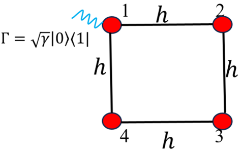
Figure 2: The 4-qubit transverse Ising model with periodic boundary conditions subjected to dissipation (amplitude damping noise). For convenience, the dissipation only acts on the first qubit.

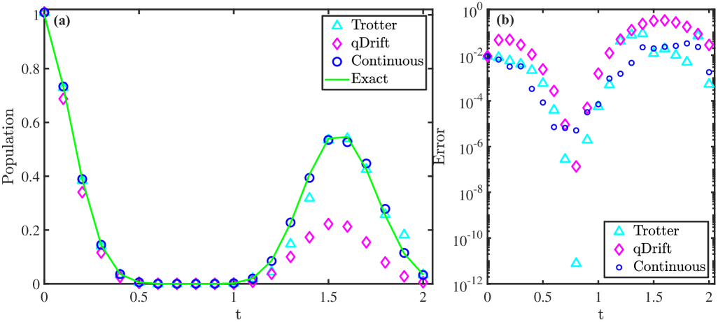
Figure 3: Dynamics simulation of a 4-qubit transverse Ising model with periodic boundary conditions subjected to dissipation. The related parameters in the model are $h=2,J=1$, the initial state $|\psi\rangle=|1000\rangle$, the population observable is $O=|1000\rangle\langle 1000|$, and the jump operator of amplitude damping noise $\Gamma=\sqrt{\gamma}|0\rangle_{1}\langle 1|$, where $\gamma=1.5$. (a) The relation between population and time $t$. The simulation duration is $T=2$. The time step of both Trotter, qDrift method is $\Delta t=0.05$, and $\tau=0.05$, the compensation coefficient $c_{p}=0.3607$, the number of samples $N_{s}=10^{5}$ in the continuous method. (b) The relation between the absolute error and time $t$. The vertical axis scale is logarithmic.

In Fig.3, we give the simulation results. The model under investigation incorporates specific parameters detailed as follows: $h=2$, $J=1$, with an initial state $|\psi\rangle=|1000\rangle$. The population observable is defined as $O=|1000\rangle\langle 1000|$. When implementing specific sampling $U(T,k)$, we used three methods, 1-order Trotter (cyan triangle), qDrift (magenta diamond), and continuous method (blue circle) respectively. The relation between population and time $t$ is given in Fig.3(a).

As seen in Fig.3(a), all three methods perform well before the simulation duration of $t=1$. However, beyond this point, the qDrift method deviates significantly from the exact values, while the other two methods exhibit better performance. This phenomenon aligns with the results presented in the Fig.3 of Ref.[44]. Moreover, it is evident that, overall, within the simulation process, the continuous method generally performs the best, only with few exceptions. This is clearly illustrated in Fig.3(b), which depicts the relation between error and time $t$. The smaller errors imply that, for a specific precision, we can utilize shallower quantum circuits. This is the primary reason we have emphasized the continuous method in the preceding text. It is important to note that, unlike the other two methods, the continuous method does not suffer from systematic errors due to time discretization. More accurately, the errors arising from time discretization in this method can be automatically mitigated by simply increasing the number of samples, thus avoiding the impact of limited resolution due to finite qubit numbers in practical quantum gates. In contrast, the other two methods inevitably suffer from systematic errors due to time discretization. It should be noted that the unusually small error observed for the Trotter method near $t=0.8$ is a fortuitous outcome.

Conclusions and discussions.—

In this work, we propose a general hybrid classical-quantum algorithmic framework based on Quantum Monte Carlo for simulating the dynamics of arbitrary time-dependent non-Hermitian systems, and present its error and complexity analyses. Theoretically, this algorithm can be applied to simulate any time-dependent non-Hermitian system dynamics, including PT-symmetric systems, non-physical processes, open quantum systems without assuming that the Hamiltonian is special, e.g. anti-Hermitian or diagonalizable like the quantum imaginary time evolution algorithm. Furthermore, our algorithm can also be regarded as a natural extension of the quantum imaginary-time evolution algorithm. This algorithm combines the advantages of both classical and quantum computation, such as requiring fewer ancillary qubits, having a shallow quantum circuit depth, and being robust against errors. To verify the effectiveness of our method, we applied it to the task of simulating open quantum systems and achieved promising results.

From an application perspective, given the good applicability and adaptability of our method, we anticipate that it will find its place in more applications, such as solving ground state energies and simulating non-physical processes. From an optimization perspective, when performing real simulations on quantum computers, Hamiltonian simulation needs to be used as a subroutine within our framework. In our application, we used the 1-order Trotter method, the qDrift method, and the continuous method as subroutines, and found that in most cases, when the number of samples is not too large, the continuous method offers greater accuracy advantages. Additionally, this method benefits even more from increasing the number of samples, which is consistent with the conclusions in Ref.[44]. Therefore, we recommend the continuous method as the preferred approach for our Hamiltonian simulation subroutine. A natural next step would be to incorporate various quantum error mitigation techniques to achieve even shallower quantum circuit depths.

Acknowledgements.—

We are grateful to Xiao Yuan for his helpful insights and discussions. This work is supported by the National Natural Science Foundation of China (Grant No. 12361161602 and No. 12175003), NSAF (Grant No. U2330201), the Innovation Program for Quantum Science and Technology (Grant No. 2023ZD0300200). Qiming Ding is supported by Beijing Natural Science Foundation (Grant No. 1254053).

Appendix A The kernel functions

Initially, Dong An et al. found and strictly proved that the kernel function can be taken as

$$f(k)=\frac{1}{\pi(1+ik)},$$ (7)

then the integrand function $g(k)=\frac{1}{\pi(1+k^{2})}$ is the standard Cauchy distribution function, and can be generated effectively and directly by the inverse transform sampling method. However, this integrand has the property: $\mathbb{E}k=0,\mathbb{E}|k|=\infty,\mathbb{E}k^{2}=\infty$, so in actual use, it is usually necessary to truncate it. Given a truncation precision $\varepsilon$, we can solve the defined truncation length $k_{c}$ in the following way:

$$\int_{-k_{c}}^{k_{c}}\left|\frac{f(k)}{1-ik}\right|dk=1-\varepsilon.$$ (8)

For the kernel function given in Eq.(7), $k_{c}=\frac{1}{\tan(\frac{\pi}{2}\varepsilon)}=\mathcal{O}(\frac{1}{\varepsilon})$.

Later, Dong An et al. put forward a set of improved kernel functions to make the integrand converge faster,

$$f(k)=\frac{2}{2\pi e^{-2\beta}e^{(1+ik)^{\beta}}},\beta\in(0,1).$$ (9)

This new kernel function decays at a near-exponential rate of $e^{-c|k|^{\beta}}$, so the truncation length can be reduced from $\mathcal{O}(1/\varepsilon)$ to $\mathcal{O}\left((\log(1/\varepsilon))^{1/\beta}\right)$. This important improvement can further reduce the circuit depth of our algorithm. However, it should be noted that in Eq.(7), $g(k)$ is real, while it is complex here, which may increase the difficulty of classical sampling. Some important classical Monte Carlo algorithms can be suggested to generate such complex samples, such as the acceptance-rejection sampling algorithm or the Metropolis algorithm, or more directly, use trapezoidal rules to generate such complex probability distributions, but this may introduce additional discretization errors.

Appendix B Proof of Theorem 1

Proof.

Considering the Eq.(Preliminaries.—), we know that

$$\langle O\rangle= \frac{\langle\psi|\mathcal{\overline{T}}e^{-i\int_{0}^{T}H^{\dagger}(s)ds}\cdot O\cdot\mathcal{T}e^{-i\int_{0}^{T}H(s)ds}|\psi\rangle}{\langle\psi|\mathcal{\overline{T}}e^{-i\int_{0}^{T}H^{\dagger}(s)ds}\cdot I\cdot\mathcal{T}e^{-i\int_{0}^{T}H(s)ds}|\psi\rangle}$$

$$= \frac{\langle\psi|\left(e^{\int_{0}^{T}{E_{i}}_{0}(s)ds}\cdot\mathcal{\overline{T}}e^{-i\int_{0}^{T}H^{\dagger}(s)ds}\right)\cdot O\cdot\left(e^{\int_{0}^{T}{E_{i}}_{0}(s)ds}\cdot\mathcal{T}e^{-i\int_{0}^{T}H(s)ds}\right)|\psi\rangle}{\langle\psi|\left(e^{\int_{0}^{T}{E_{i}}_{0}(s)ds}\cdot\mathcal{\overline{T}}e^{-i\int_{0}^{T}H^{\dagger}(s)ds}\right)\cdot I\cdot\left(e^{\int_{0}^{T}{E_{i}}_{0}(s)ds}\cdot\mathcal{T}e^{-i\int_{0}^{T}H(s)ds}\right)|\psi\rangle}$$

$$= \frac{\langle\psi|\mathcal{\overline{T}}e^{-i\int_{0}^{T}\tilde{H}^{\dagger}(s)ds}\cdot O\cdot\mathcal{T}e^{-i\int_{0}^{T}\tilde{H}(s)ds}|\psi\rangle}{\langle\psi|\mathcal{\overline{T}}e^{-i\int_{0}^{T}\tilde{H}^{\dagger}(s)ds}\cdot I\cdot\mathcal{T}e^{-i\int_{0}^{T}\tilde{H}(s)ds}|\psi\rangle}$$

$$= \frac{\langle\psi|\int_{\mathbb{R}}g^{*}(k^{\prime})[\mathcal{\overline{T}}e^{i\int_{0}^{T}K_{s^{\prime}}(k^{\prime})ds^{\prime}}]dk^{\prime}\cdot O\cdot\int_{\mathbb{R}}g(k)[\mathcal{T}e^{-i\int_{0}^{T}K_{s}(k)ds}]dk|\psi\rangle}{\langle\psi|\int_{\mathbb{R}}g^{*}(k^{\prime})[\mathcal{\overline{T}}e^{i\int_{0}^{T}K_{s^{\prime}}(k^{\prime})ds^{\prime}}]dk^{\prime}\cdot I\cdot\int_{\mathbb{R}}g(k)[\mathcal{T}e^{-i\int_{0}^{T}K_{s}(k)ds}]dk|\psi\rangle}$$

$$= \frac{\|O\|_{l_{1}}\cdot\mathbb{E}_{n}\int_{\mathbb{R}}\int_{\mathbb{R}}g^{*}(k^{\prime})g(k)\cdot\langle O_{n}(k^{\prime},k)\cdot e^{i\theta(n)}\rangle\cdot dk^{\prime}dk}{\int_{\mathbb{R}}\int_{\mathbb{R}}g^{*}(k^{\prime})g(k)\cdot\langle I(k^{\prime},k)\rangle\cdot dk^{\prime}dk}$$

$$= \frac{\|O\|_{l_{1}}\cdot\|g\|_{1}^{2}\cdot\mathbb{E}_{n,k^{\prime},k}\langle O_{n}(k^{\prime},k)\cdot e^{i\theta(n)}\cdot e^{i\theta(k^{\prime},k)}\rangle}{\|g\|_{1}^{2}\cdot\mathbb{E}_{k^{\prime},k}\langle I(k^{\prime},k)\cdot e^{i\theta(k^{\prime},k)}\rangle}$$

$$= \frac{\|O\|_{l_{1}}\cdot\mathbb{E}_{k^{\prime},k,n}\langle O_{n}(k^{\prime},k)\cdot e^{i\theta(n)}\cdot e^{i\theta(k^{\prime},k)}\rangle}{\mathbb{E}_{k^{\prime},k}\langle I(k^{\prime},k)\cdot e^{i\theta(k^{\prime},k)}\rangle}.$$ (10)

Noting that when $\tilde{H}$ is time-independent, $\langle[\cdot](k^{\prime},k)\rangle=\langle\psi|e^{iK(k^{\prime})T}[\cdot]e^{-iK(k)T}|\psi\rangle$. ∎

Appendix C Proof of Theorem 2 (Error and complexity analysis)

Proof.

In the following, we present the error and complexity analysis, thus completing the proof of Theorem 2.

C.0.1 Truncation error, quadrature error and the query complexity

According to the conclusions of Lemma 9 in Ref.[58], we know that the truncation error incurred in approximating the non-unitary evolution $\mathcal{T}e^{-i\int_{0}^{T}\tilde{H}(s)ds}$ in theorem 2 can be bounded as

$$\left\|\int_{\mathbb{R}}g(k)U(T,k)\mathrm{d}k-\int_{-k_{c}}^{k_{c}}g(k)U(T,k)\mathrm{d}k\right\|\leq\frac{2^{\lceil 1/\beta\rceil+1}\lceil 1/\beta\rceil!}{C_{\beta}(\cos(\beta\pi/2))^{\lceil 1/\beta\rceil}}\frac{1}{k_{c}}e^{-\frac{1}{2}{k_{c}}^{\beta}\cos(\beta\pi/2)},$$ (11)

where $c_{\beta}=2\pi e^{-2^{\beta}}$, and $U(T,k)=\mathcal{T}e^{-i\int_{0}^{T}[H_{r}(s)+k(H_{i}(s)-{E_{i}}_{0}(s))]\mathrm{d}s}$.

To bound the above truncation error by $\varepsilon$, make the right-hand side of the above equation to be less than or equal to $\epsilon$, then we can obtain

$$k_{c}=\mathcal{O}\left(\left(\log\left(\frac{1}{\varepsilon}\right)\right)^{1/\beta}\right),$$ (12)

which is seen as the query complexity of our algorithm when the Hamiltonian $\tilde{H}(t)$ is time-independent.

In addition, when the Hamiltonian $\tilde{H}$ is time-dependent, the evolution operator typically contains a time-ordering operator $\mathcal{T}$, necessitating a discretization of time, which inevitably introduces an additional error commonly referred to as the quadrature error. According to the conclusions of Lemma 10 in Ref.[58], the quadrature error can be bounded as

$$\left\|\int_{-k_{c}}^{k_{c}}g(k)U(T,k)\mathrm{d}k-\sum_{m=-k_{c}/h}^{k_{c}/h-1}\sum_{q=0}^{Q-1}c_{q,m}U\left(T,k_{q,m}\right)\right\| \leqslant\frac{8}{3C_{\beta}}k_{c}h^{2Q}\left(\frac{eT\max_{t}\|\tilde{H}_{i}(t))\|}{2}\right)^{2Q}$$

$$\leqslant\frac{8}{3C_{\beta}}k_{c}h^{2Q}\left(\frac{eT\max_{t}\|\tilde{H}(t)\|}{2}\right)^{2Q}.$$ (13)

In the above equation, the Gauss-Legendre quadrature is utilized, where $Q$ denotes the number of quadrature nodes. Here, $h$ is the step size used in the composite quadrature rule, and $h$ can be chosen to be a suitable value such that $k_{c}/h$ is an integer. And the $k_{q,m}$’s are the Gaussian nodes, $c_{q,m}=w_{q}g(k_{q,m})$, and the $w_{q}$’s are the Gaussian weights. It is worth emphasizing that both $k_{q,m}$ and $w_{q}$ can be considered as known quantities (by consulting tables), which are retrieved through the Gauss-Legendre quadrature methods.

By bounding the above quadrature error by $\varepsilon$, the parameter values can be obtained as

$$h=\frac{1}{eT\max_{t}\|\tilde{H}(t)\|},\quad Q=\left\lceil\frac{1}{\log 4}\log\left(\frac{8}{3C_{\beta}}\frac{k_{c}}{\varepsilon}\right)\right\rceil=\mathcal{O}\left(\log\left(\frac{1}{\varepsilon}\right)\right),$$ (14)

so the overall number of unitaries $U(T,k_{q,m})$ in the Eq.(C.0.1) is

$$M=\frac{2k_{c}Q}{h}=\mathcal{O}\left(T\max_{t}\|\tilde{H}(t)\|\left(\log\left(\frac{1}{\varepsilon}\right)\right)^{1+1/\beta}\right),$$ (15)

which can be seen as the query complexity of our algorithm when the Hamiltonian $\tilde{H}(t)$ is time-dependent.

C.0.2 Statistical error and the sampling complexity

Next, we will discuss estimating the numerator and the denominator in Eq.(3) (the numerator is recorded as $N(O)$ here and hereafter, the denominator can be regarded as $N(I)$, but for the sake of easy distinction, we also denote it as $D$). Recalling that

$$\hat{N}(O) =\|g\|_{1}^{2}\cdot\langle O(k^{\prime},k)\cdot e^{i\theta(k^{\prime},k)}\rangle,$$

$$\overline{\hat{N}}(O) =\frac{1}{n_{N}}\sum_{i=1}^{n_{N}}\hat{N}(O),$$ (16)

where $n_{N}$ denotes $n_{N}$ independent sampling processes with independent identical distribution $\mathrm{Pd}(\cdot)$ ($\mathrm{Pd}(k^{\prime},k)=\mathrm{Pd}(k^{\prime})\cdot\mathrm{Pd}(k)$), so it is obvious $\mathbb{E}{\overline{\hat{N}}(O)}=N(O)$. For convenience, we have omitted the parameters $k^{\prime}$ and $k$. Then the estimator of $\langle O\rangle$ can be denoted by $\langle\hat{O}\rangle\equiv\overline{\hat{N}}(O)/\overline{\hat{D}}$.

$\hat{N}(O)$ and $\overline{\hat{N}}(O)$ are usually complex numbers, and their estimation needs to be divided into real part $\Re[\cdot]$ and imaginary part $\Im[\cdot]$ separately. For the estimation precision $\epsilon_{N}$ of $N(O)$ ($N(I)$), according to the Hoeffding inequality (see the Eq.(111) in Ref.[56]), and considering that $\Re\overline{\hat{N}}(O)$, $\Im\overline{\hat{N}}(O)$, $\in\left[-\|g\|_{1}^{2}\cdot\|O\|_{l_{1}},\quad\|g\|_{1}^{2}\cdot\|O\|_{l_{1}}\right]$, we know

$$\mathrm{Pr}(|\Re\overline{\hat{N}}(O)-\mathbb{E}\Re\overline{\hat{N}}(O)| \geqslant\epsilon_{N,\mathrm{Re}})\leqslant 2\exp{\left(-\frac{n_{N,\mathrm{Re}}\cdot\epsilon_{N,\mathrm{Re}}^{2}}{2\|g\|_{1}^{4}\cdot\|O\|_{l_{1}}^{2}}\right)},$$

$$\mathrm{Pr}(|\Im\overline{\hat{N}}(O)-\mathbb{E}\Im\overline{\hat{N}}(O)| \geqslant\epsilon_{N,\mathrm{Im}})\leqslant 2\exp{\left(-\frac{n_{N,\mathrm{Im}}\cdot\epsilon_{N,\mathrm{Im}}^{2}}{2\|g\|_{1}^{4}\cdot\|O\|_{l_{1}}^{2}}\right)},$$ (17)

so the sample number of the numerator will be

$$n_{N,\rm{Re}}\geqslant\frac{K_{N,\mathrm{Re}}\cdot\|g\|_{1}^{4}\|O\|_{l_{1}}^{2}}{\epsilon_{N,\mathrm{Re}}^{2}},$$

$$n_{N,\rm{Im}}\geqslant\frac{K_{N,\mathrm{Im}}\cdot\|g\|_{1}^{4}\|O\|_{l_{1}}^{2}}{\epsilon_{N,\mathrm{Im}}^{2}},$$ (18)

with a failure probability

$$\delta_{N,\mathrm{Re}}\leqslant 2\exp{\left(-\frac{K_{N,\mathrm{Re}}}{2}\right)},$$

$$\delta_{N,\mathrm{Im}}\leqslant 2\exp{\left(-\frac{K_{N,\mathrm{Im}}}{2}\right)},$$ (19)

where $K_{N,\rm{Re}}>0$ and $K_{N,\rm{Im}}>0$ represent the manually chosen parameter that regulates both the quantity of samples and the failure probability. Usually, we can set $\epsilon_{N,\rm{Re}}=\epsilon_{N,\rm{Im}}=\epsilon_{N}/\sqrt{2}$, $K_{N,\rm{Re}}=K_{N,\rm{Im}}=K_{N}$, and $\delta_{N,\mathrm{Re}}=\delta_{N,\mathrm{Im}}=\delta_{N}/2$, then

$$\mathrm{Pr}(|\overline{\hat{N}}(O)-N(O)|\geqslant\epsilon_{N})\leqslant 1-(1-\delta_{N,\rm{Re}})(1-\delta_{N,\rm{Im}})\leqslant\delta_{N}.$$ (20)

Overall, taking into account the failure probabilities of numerator $N(O)$ estimation and denominator $D$ estimation, the estimated failure probability for $\langle O\rangle=N(O)/D(O)$ is

$$\delta\leqslant 1-(1-\delta_{D})(1-\delta_{N})\leqslant 4\exp{(-\frac{K_{D}}{2})}+4\exp{(-\frac{K_{N}}{2})}.$$ (21)

Traditionally, we often take $K_{D}=K_{N}$, then $K_{D}=K_{N}\leqslant 2\ln(8/\delta)$.

Following an analysis of the sampling complexity associated with both the numerator and the denominator, an estimation of the total error for $\langle O\rangle$ can be carried out,

$$\left|\langle O\rangle-\langle\hat{O}\rangle\right| =\left|\frac{N(O)}{D}-\frac{\overline{\hat{N}}(O)}{\overline{\hat{D}}}\right|$$

$$=\left|\frac{N(O)\overline{\hat{D}}-D\overline{\hat{N}}(O)}{D\hat{D}}\right|$$

$$=\left|\frac{N(O)\left(D+(\overline{\hat{D}}-D)\right)-D\left(N(O)-(\overline{\hat{N}}(O)-N(O))\right)}{D\left(D+(\overline{\hat{D}}-D)\right)}\right|$$

$$=\left|\frac{N(O)(\overline{\hat{D}}-D)+D\left(\overline{\hat{N}}(O)-N(O)\right)}{D\left(D+(\overline{\hat{D}}-D)\right)}\right|$$

$$=\left|\frac{\langle O\rangle(\overline{\hat{D}}-D)+\left(\overline{\hat{N}}(O)-N(O)\right)}{D+(\overline{\hat{D}}-D)}\right|$$

$$\leqslant\frac{|\langle O\rangle|\epsilon_{D}+\epsilon_{N}}{D-\epsilon_{D}}$$

$$\leqslant\frac{(|\langle O\rangle|+1)\epsilon_{D}+\epsilon_{N}}{D}$$

$$\leqslant\frac{(\|O\|_{l_{1}}+1)\epsilon_{D}+\epsilon_{N}}{D},$$ (22)

where we have reasonably assumed that $\epsilon_{D}<D$. In practice, $\epsilon_{D}$ is usually taken as $\epsilon$, $\epsilon_{N}$ is usually taken as $\|O\|_{l_{1}}\epsilon$, so in order to make the above upper bound of the error smaller or equal to the permissible error $\eta$ synthesized by the numerator and the denominator, it should be satisfied that

$$\epsilon\leqslant\frac{D}{(2\|O\|_{l_{1}}+1)}\eta\Longrightarrow\epsilon_{D}\leqslant\frac{D}{(2\|O\|_{l_{1}}+1)}\eta,\epsilon_{N}\leqslant\frac{\|O\|_{l_{1}}D}{(2\|O\|_{l_{1}}+1)}\eta.$$ (23)

Then according to Eq.(C.0.2) we know that $n_{D}$, $n_{N}$ should meet the following condition

$$n_{D,\rm{Re}} \geqslant\frac{K_{D,\rm{Re}}\cdot\|g\|_{1}^{4}\|I\|_{l_{1}}^{2}}{\epsilon_{D,\rm{Re}}^{2}}=\frac{K_{D,\rm{Re}}\cdot(2\|O\|_{l_{1}}+1)^{2}\|g\|_{1}^{4}}{2D^{2}\eta^{2}},$$

$$n_{D,\rm{Im}} \geqslant\frac{K_{D,\rm{Im}}\cdot\|g\|_{1}^{4}\|I\|_{l_{1}}^{2}}{\epsilon_{D,\rm{Im}}^{2}}=\frac{K_{D,\rm{Im}}\cdot(2\|O\|_{l_{1}}+1)^{2}\|g\|_{1}^{4}}{2D^{2}\eta^{2}},$$

$$n_{N,\rm{Re}} \geqslant\frac{K_{N,\rm{Re}}\cdot\|g\|_{1}^{4}\|O\|_{l_{1}}^{2}}{\epsilon_{N,\rm{Re}}^{2}}=\frac{K_{N,\rm{Re}}\cdot(2\|O\|_{l_{1}}+1)^{2}\|g\|_{1}^{4}}{2D^{2}\eta^{2}},$$

$$n_{N,\rm{Im}} \geqslant\frac{K_{N,\rm{Im}}\cdot\|g\|_{1}^{4}\|O\|_{l_{1}}^{2}}{\epsilon_{N,\rm{Im}}^{2}}=\frac{K_{N,\rm{Im}}\cdot(2\|O\|_{l_{1}}+1)^{2}\|g\|_{1}^{4}}{2D^{2}\eta^{2}}.$$ (24)

In addition, form the property of the norm we know that

$$e^{-2\int_{0}^{T}({E_{i}}_{max}(s)-{E_{i}}_{0}(s))ds}\leqslant D=\langle\psi|\mathcal{\overline{T}}e^{-i\int_{0}^{T}\tilde{H}^{\dagger}(s)ds}\cdot I\cdot\mathcal{T}e^{-i\int_{0}^{T}\tilde{H}(s)ds}|\psi\rangle\leqslant e^{-2\int_{0}^{T}({E_{i}}_{min}(s)-{E_{i}}_{0}(s))ds},$$

where ${E_{i}}_{min(max)}(s)$ is the minimum (maximum) eigenvalue of $H_{i}(s)$, and in fact, ${E_{i}}_{min}(s)$ is the ground state eigenvalue of $H_{i}(s)$, and they can always be estimated within a reasonable interval by some algorithms [66, 42, 67]. Denoting that $E_{avg}(T)=\int_{0}^{T}({E_{i}}_{max}(s)-{E_{i}}_{min}(s))ds/T\leqslant\Delta_{E_{i}}$, where $\Delta_{E_{i}}=\underset{s\in[0,T]}{\max}\{{E_{i}}_{max}(s)-{E_{i}}_{min}(s)\}$. It is worth noting that $E_{avg}(T)$ is a structural constant of the system $H(t)$, and its physical meaning is the average bandwidth of the anti-Hermitian part of the Hamiltonian $H(t)$, and $\Delta_{E_{i}}$ represents the maximum bandwidth of $H_{i}(t)$.

Considering ${E_{i}}_{min}(s)-{E_{i}}_{0}(s)\geqslant 0$, and the failure probability given in Eq.(C.0.2) and Eq.(21). Then the maximum sampling number can be taken as

$$n_{D} =\frac{2\ln(\frac{8}{\delta})\cdot(2\|O\|_{l_{1}}+1)^{2}\|g\|_{1}^{4}e^{4T\Delta_{E_{i}}}}{\eta^{2}}=\mathcal{O}\left(\frac{\log(\frac{1}{\delta})\cdot(\|O\|_{1}+1)^{2}\|g\|_{1}^{4}}{\eta^{2}}\right),$$

$$n_{N} =\frac{2\ln(\frac{8}{\delta})\cdot(2\|O\|_{l_{1}}+1)^{2}\|g\|_{1}^{4}e^{4T\Delta_{E_{i}}}}{\eta^{2}}=\mathcal{O}\left(\frac{\log(\frac{1}{\delta})\cdot(\|O\|_{l_{1}}+1)^{2}\|g\|_{1}^{4}}{\eta^{2}}\right),$$ (26)

where we have assumed that the duration of the algorithm is $T=\mathcal{O}(1/\Delta_{E_{i}})$. The Eqs.(C.0.2) are the sampling complexity when the Hamiltonian $H$ is time-dependent.

From Eqs.(C.0.2), it can be seen that the number of samples typically required increases exponentially with duration $T$, which is inherently an NP-hard problem. A similar issue arises in quantum imaginary-time evolution algorithms [42]. Therefore, for general non-Hermitian systems $H$, we set the duration of our algorithm to $T=\mathcal{O}(1/\Delta_{E_{i}})$ to circumvent this problem.

Specially, when $H$ is time-independent,

$$D\geqslant e^{-2({E_{i}}_{min}-{E_{i}}_{0})T}\cdot p_{g},$$

where $p_{g}\equiv|\langle\phi_{g}|\psi\rangle|^{2}$ is the overlap between the ground state eigenvalue $|\phi_{g}\rangle$ of $H_{i}$ and the initial state $|\psi\rangle$, ${E_{i}}_{0}$ can be chosen to ensure $({E_{i}}_{min}-{E_{i}}_{0})T=\log(\mathcal{O}(1))$, then the maximum sampling number can be bounded by

$$n_{D} =\mathcal{O}\left(\frac{\log(\frac{1}{\delta})\cdot(\|O\|_{l_{1}}+1)^{2}\|g\|_{1}^{4}}{\eta^{2}p_{g}^{2}}\right),$$

$$n_{N} =\mathcal{O}\left(\frac{\log(\frac{1}{\delta})\cdot(\|O\|_{l_{1}}+1)^{2}\|g\|_{1}^{4}}{\eta^{2}p_{g}^{2}}\right).$$ (28)

∎

Appendix D The subroutine for Hamiltonian simulation without time discretization error

In this section, we review a Hamiltonian dynamics simulation method without discretization error proposed by Etienne Granet and Henrik Dreyer, and this method belongs to the category of Quantum Monte Carlo methods [44]. The emphasis on this continuous method stems from three primary factors: Firstly, it is theoretically devoid of systematic errors resulting from time discretization. Specifically, when compared to other Quantum Monte Carlo algorithms (such as qDrift, qSwift, QCMC, etc), increasing the number of samples not only effectively mitigates statistical errors but also systematically reduces errors stemming from time discretization. Secondly, this method can suppress systematic errors caused by the finite resolution of quantum gates and is theoretically immune to such errors. Lastly, in practical scenarios involving noisy quantum computers, this method has demonstrated potential exponential advantages in terms of precision dependence. These characteristics will collectively render this algorithm highly competitive in the NISQ era. We will see the effect of using this continuous method in Fig.3.

Given a Hermitian Hamiltonian $H(t)=\sum_{n}c_{n}\sigma_{n}$, where $\sigma_{n}=\{I,X,Y,Z\}^{\otimes n}$ is generalized pauli operators, and $\{c_{n}\}$ are real. For any rotation Pauli gate operation, it can always be regarded as the rotation Pauli gate operation with bigger angle, but with a certain probability and an attenuation (gain). If this principle is written in the form of an equation, that is

$$(1+p)I+p\cdot e^{-i|c|\cdot\mathrm{sgn}(c)\sigma\cdot\tau}=\lambda e^{-ic\sigma\cdot d\tau^{\prime}},$$ (29)

where the angle $|c|\tau>|c|d\tau^{\prime}>0$, $c\in\mathbb{R}$ and $\lambda$ is the attenuation coefficient. The purpose of setting the sign function ’sgn’ on the left side of the equation above is to ensure that the probability $p$ is always positive. Solving the above Eq.(29),

$$p =\frac{\tan(|c|d\tau^{\prime})}{\sin\tau+(1-\cos\tau)\tan{d\tau^{\prime}}}$$

$$=\frac{|c|d\tau^{\prime}}{\sin\tau}+\mathcal{O}({(d\tau^{\prime})^{2}}),\quad|c|d\tau^{\prime}\rightarrow 0^{+},$$

$$\lambda =\frac{p\sin\tau}{\sin\tau^{\prime}}$$

$$=\frac{1}{\cos{d\tau^{\prime}}\cdot(1+\tan{|c|d\tau^{\prime}}\cdot\tan(\frac{\tau}{2}))}$$

$$=1-d\tau^{\prime}\cdot|c|\tan\frac{\tau}{2}+\mathcal{O}({(d\tau^{\prime})^{2}}),\quad|c|d\tau^{\prime}\rightarrow 0^{+}.$$ (30)

Recalling that the definition of Poisson process,

Definition 1.

A stochastic process $\{N(t),t\geqslant 0\}$ is called a time homogeneous Poisson process (referred to as a Poisson process for short) if it satisfies:
(1) a counting process, and N (0)=0;
(2) an independent incremental process, that is, for any $0<t_{1}<t_{2}<\textperiodcentered\textperiodcentered\textperiodcentered\textperiodcentered\textperiodcentered<t_{n}$, $N(t_{1}),N(t_{2})-N(t_{1}),..,N(ta_{n})-N(t_{n-1})$ are mutual independence;
(3) Incremental smoothness, i.e. $\forall s,t\geqslant 0,n\geqslant 0$, the probability $p[N(s+t)-N(s)=n]=p[N(t)=n]$;
(4) For any $t>0$ and sufficiently small $\Delta t>0$, $p[N(t+\Delta t)-N(t)=1]=\alpha\cdot\Delta t+o(\Delta t)$ ($\alpha>0$), and $P[N(t+\Delta t)-N(t)\geqslant 2|=o(\Delta t)$,

so the process given in the Eq.(29) is actually a Poisson process, except for a coefficient $\lambda$. Then multiplying the two sides of the Eq.(29) by $M$ times while setting $M\cdot d\tau^{\prime}\rightarrow T$, and according to the Eq.(D), then the Eq.(29) becomes

$$[(1+p)I+p\cdot e^{-i|c|\cdot\mathrm{sgn}(c)\sigma\cdot\tau}]^{M}=[\lambda e^{-ic\sigma\cdot d\tau^{\prime}}]^{M}\rightarrow\lambda_{tot}e^{-ic\sigma\cdot T},\quad\lambda_{tot}=e^{-T\sum_{n}\cdot|c_{n}|\tan(\tau_{n}/2)}.$$ (31)

The left side of the above Eq.(31) meets the binomial distribution $B(M,p)$, and as we all know, when $M\rightarrow\infty$, while $p\rightarrow 0^{+}$, the binomial distribution will be transformed into Poisson distribution, i.e., $B(M,p)\rightarrow Poi(M\cdot p)=Poi(\frac{|c|T}{\sin\tau})$, where we have used the results of the Eq.(D). Therefore, when we consider the Hamiltonian simulation task,

$$e^{-iH\cdot T}=\lim_{d\tau^{\prime}\to 0^{+}}(e^{-ic_{1}\sigma_{1}\cdot d\tau^{\prime}}e^{-ic_{2}\sigma_{2}\cdot d\tau^{\prime}}...e^{-ic_{N}\sigma_{N}\cdot d\tau^{\prime}})^{T/d\tau^{\prime}},$$ (32)

and according to the principle we introduced, we know that each small angle rotating Pauli gates {$e^{-ic_{n}\sigma_{n}\cdot d\tau^{\prime}}$} can be decomposed into a larger angle rotating Pauli gates {$e^{-i|c_{n}|\cdot\mathrm{sgn}(c_{n})\sigma_{n}\cdot d\tau^{\prime}}$} with multiplying the constant coefficient $1/\lambda_{n}$ (the total attenuation coefficient will be $\lambda_{tot}=e^{-T\cdot\sum|c_{n}|\tan(\tau_{n}/2)})$, and the number of times they appear in time intervals $[0,T]$ follows the Poisson distribution $\mathrm{Poi}(\frac{|c_{n}|T}{\sin\tau_{n}})$. Furthermore, according to the property of Poisson distribution, we know that the occurrence time of these gates $\{e^{-i|c_{n}|\cdot\mathrm{sgn}(c_{n})\sigma_{n}\cdot d\tau^{\prime}}\}$ will follow the uniform distribution $U(0,T)$ between time intervals [0, T]. By arranging all the rotated Pauli gates generated through sampling in ascending order of time, the quantum gate sequence is generated, denoted as $V$. Since the generation of each type of gate is independent of each other, the total number of gates in $V$ satisfies the Poisson distribution $\mathrm{Poi}(T\sum_{n}\frac{|c_{n}|}{\sin\tau_{n}})$, and

$$e^{-iHT}=\frac{1}{\lambda_{tot}}\cdot\mathbb{E}V=e^{T\cdot\sum_{n}|c_{n}|\tan\frac{\tau_{n}}{2}}\cdot\mathbb{E}V,$$ (33)

where the symbol ’$\mathbb{E}$’ represents the expectation, and $\lambda_{tot}$ has been defined in Eq.(31).

It is worth noting that this theory is also applicable to the case where the system is time-dependent. All that is needed is to change all the output parameters related to time cumulants from products to integrals with respect to time, such as $\mathrm{Poi}(T\sum_{n}\frac{|c_{n}|}{\sin\tau_{n}})\rightarrow\mathrm{Poi}(\sum_{n}\int_{0}^{T}\frac{|c_{n}(s)|}{\sin\tau_{n}}\mathrm{d}s)$, $\lambda_{tot}=e^{-T\cdot\sum_{n}|c_{n}|\tan(\tau_{n}/2)}\rightarrow\lambda_{tot}=e^{-\sum_{n}\int_{0}^{T}|c_{n}(s)|\tan(\tau_{n}/2)\mathrm{d}s}$. Within this Hamiltonian simulation method, our scheme given in Eq.(3) further evolves as follows:

$$\langle O\rangle= \frac{\langle\psi|\mathcal{\overline{T}}e^{-i\int_{0}^{T}\tilde{H}^{\dagger}(s)ds}\cdot O\cdot\mathcal{T}e^{-i\int_{0}^{T}\tilde{H}(s)ds}|\psi\rangle}{\langle\psi|\mathcal{\overline{T}}e^{-i\int_{0}^{T}\tilde{H}^{\dagger}(s)ds}\cdot I\cdot\mathcal{T}e^{-i\int_{0}^{T}\tilde{H}(s)ds}|\psi\rangle}$$

$$= \frac{\lambda_{tot}^{-2}\cdot\|g\|\cdot\mathbb{E}_{V^{\prime},V}\mathbb{E}_{k^{\prime},k,n}\langle{O_{n}}_{V^{\prime},V}(k^{\prime},k)\cdot e^{is(k^{\prime},k)})\rangle}{\lambda_{tot}^{-2}\cdot\|g\|\cdot\mathbb{E}_{V^{\prime},V}\mathbb{E}_{k^{\prime},k}\langle I_{V^{\prime},V}(k^{\prime},k)\cdot e^{is(k^{\prime},k)}\rangle}$$

$$= \frac{\mathbb{E}_{V^{\prime},V}\mathbb{E}_{k^{\prime},k,n}\langle{O_{n}}_{V^{\prime},V}(k^{\prime},k)\cdot e^{is(k^{\prime},k)})\rangle}{\mathbb{E}_{V^{\prime},V}\mathbb{E}_{k^{\prime},k}\langle I_{V^{\prime},V}(k^{\prime},k)\cdot e^{is(k^{\prime},k)}\rangle},$$ (34)

where we continue to derive along the conclusion in Eq.(3), $\langle[\cdot](k^{\prime},k)\rangle\equiv\langle\psi|\mathcal{\overline{T}}e^{i\int_{0}^{T}K_{s}^{\prime}(k^{\prime})ds^{\prime}}[\cdot]\mathcal{T}e^{-i\int_{0}^{T}K_{s}(k)ds}|\psi\rangle=\lambda_{tot}^{-2}\cdot\mathbb{E}_{V^{\prime},V}\langle\psi|[\cdot]_{V^{\prime},V}|\psi\rangle$, $\langle\psi|[\cdot]_{V^{\prime},V}|\psi\rangle\equiv\langle\psi|V^{\prime\dagger}[\cdot]V|\psi\rangle$, $\mathbb{E}_{V^{\prime},V}$ represents the expectation with respect to $V^{\prime}$ and $V$ operators generated by the method given above the Eq.(33), and $\lambda_{tot}$ is also defined in Eq.(31) and bellow Eq.(33).

Appendix E The measurements of $N(O)$ and $D$

Next, we given the quantum circuit diagram for implementing $N(O)$. The circuit diagram for measuring numerator estimator $\hat{N}(O)$ is shown in Fig.1. In the Fig.1, $U(T,k)$ and $U(T,k^{\prime})$ are the subroutines of Hamiltonian simulation, which can be seen as black boxes, and can be implemented by any Hamiltonian simulation program. The rand number $k$, $k^{\prime}$, and $O_{n}$ are generated by a sampling program according to the probability density function $\mathrm{Pd}(k)$ and the probability $p_{n}$ given bellow Eq.(3), and the phase part of sampling $e^{is(k,k^{\prime})}$ and $e^{is(n)}$ should be finally multiplied in the calculation result. When the initial state $|\psi\rangle$ passed through this quantum circuit, we have

$$|\Psi_{n}\rangle=\frac{1}{\sqrt{2}}(|0\rangle\otimes O_{n}\cdot U(T,k)|\psi\rangle+|1\rangle\otimes U(T,k^{\prime})|\psi\rangle).$$ (35)

Therefore,

$$\langle\Psi_{n}|X|\Psi_{n}\rangle =\mathrm{Re}\left(\langle\psi|(U^{\dagger}(T,k^{\prime})\cdot O_{n}\cdot U(T,k)|\psi\rangle\right)$$

$$=\mathrm{Re}\langle O_{n}(k,k^{\prime})\rangle,$$

$$\langle\Psi_{n}|Y|\Psi_{n}\rangle =-\mathrm{Im}\left(\langle\psi|(U^{\dagger}(T,k^{\prime})\cdot O_{n}\cdot U(T,k)|\psi\rangle\right)$$

$$=-\mathrm{Im}\langle O_{n}(k,k^{\prime})\rangle.$$ (36)

After that, the estimator $\hat{N}(O)$ given in Eq.(C.0.2) can be obtained by calculating

$$\hat{N}(O)=\|g\|_{1}^{2}\cdot\sum_{n}\left(\langle\Psi_{n}|X|\Psi_{n}\rangle-i\langle\Psi_{n}|Y|\Psi_{n}\rangle\right)\cdot e^{\theta(k,k^{\prime})},$$ (37)

and then

$$N(O)=\|g\|_{1}^{2}\cdot\mathbb{E}_{k^{\prime},k}\langle O(k^{\prime},k)\cdot e^{i\theta(k^{\prime},k)}\rangle.$$ (38)

The algorithm for estimating $N(O)$ (or $D$) is given in Algorithm 1.

Appendix F The isomorphic relation between open quantum systems and non-Hermitian systems with vectorization

The Lindbald superoperator $\mathcal{L}$ in Eq.(5) will be mapped to

$$\overline{\overline{\mathcal{L}}}(t)=-i[{H}(t)\otimes I-I\otimes H^{\mathrm{T}}(t)]+\sum_{\mu}{[\Gamma_{\mu}\otimes({\Gamma^{\dagger}_{\mu}})^{\mathrm{T}}-\frac{\Gamma^{\dagger}_{\mu}\Gamma_{\mu}\otimes I}{2}-\frac{I\otimes({\Gamma^{\dagger}_{\mu}\Gamma_{\mu}})^{\mathrm{T}}}{2}]}.$$ (39)

After that the Eq.(5) will be mapped to

$$\frac{\mathrm{d}|\rho(t)\rangle\!\rangle}{\mathrm{d}t}=-iL(t)|\rho(t)\rangle\!\rangle,$$ (40)

where we have rewritten $\overline{\overline{\mathcal{L}}}$ as $-iL(t)$ to make the above equation a Schrödinger-like equation. Then we can get the solution of the above equation,

$$|\rho(t)\rangle\!\rangle=\mathcal{T}e^{-i\int_{0}^{t}L(\tau)\mathrm{d}\tau}|\rho(0)\rangle\!\rangle,$$ (41)

where $|\rho(0)\rangle\!\rangle$ is the vectorization of the initial density operator $\rho(0)$.

Meanwhile, in the context of vectorization, for the mean value of any observable $O$,

$$\langle O\rangle =\mathrm{Tr}(O\rho(t))$$

$$=\langle\!\langle O^{\dagger}|\mathcal{T}e^{-i\int_{0}^{t}L(\tau)\mathrm{d}\tau}|\rho(0)\rangle\!\rangle$$

$$=(\||O^{\dagger}\rangle\!\rangle\|\cdot\||\rho(0)\rangle\!\rangle\|)\cdot\langle O^{\dagger}|\mathcal{T}e^{-i\int_{0}^{t}L(\tau)\mathrm{d}\tau}|\rho(0)\rangle$$

$$=(\|O\|_{F}\cdot\|\rho(0)\|_{F})\cdot\langle O^{\dagger}|\mathcal{T}e^{-i\int_{0}^{t}L(\tau)\mathrm{d}\tau}|\rho(0)\rangle.$$ (42)

It is worth noting that when $O$ is a Hermitian operator, $O^{\dagger}$ in the above Eq.(F) can be replaced by $O$, at the same time, $O$ and $\rho(0)$, so $\langle\!\langle O^{\dagger}|$ and $|\rho(0)\rangle\!\rangle$, are given in the beginning. Meanwhile, according to Eq.(Preliminaries.—), the evolution operator $\mathcal{T}e^{\int_{0}^{t}-iL(\tau)\mathrm{d}\tau}$ can be implemented, therefore, the problem of the dynamics simulation of open quantum systems may be addressed. Specially, in the similar way with the Eq.(1), $L(t)$ in the Eq.(40) can be written as

$$L(t)=L_{r}(t)-iL_{i}(t),$$ (43)

where

$$L_{r}= \frac{L+L^{\dagger}}{2}=H\otimes I-I\otimes H^{\mathrm{T}}+\frac{i}{2}\sum_{\mu}[\Gamma_{\mu}\otimes(\Gamma_{\mu}^{\dagger})^{\mathrm{T}}-\Gamma_{\mu}^{\dagger}\otimes\Gamma_{\mu}^{\mathrm{T}}],$$

$$L_{i}= i\frac{L+L^{\dagger}}{2}=\frac{1}{2}\sum_{\mu}[\Gamma_{\mu}^{\dagger}\Gamma_{\mu}\otimes I+I\otimes(\Gamma_{\mu}^{\dagger}\Gamma_{\mu})^{\mathrm{T}}-\Gamma_{\mu}\otimes(\Gamma^{\dagger}_{\mu})^{\mathrm{T}}-\Gamma^{\dagger}_{\mu}\otimes\Gamma_{\mu}^{\mathrm{T}}].$$ (44)

We must emphasize that, in fact, most of the time $L_{i}$ does not satisfy the condition $L_{i}\geqslant 0$. Therefore, we have to choose a constant $c_{p}$ such that $L_{i}+c_{p}\geqslant 0$. Then according to Eq.(Preliminaries.—), Eq.(F) will become

$$\langle O\rangle=(\||O^{\dagger}\rangle\!\rangle\|\cdot\||\rho(0)\rangle\!\rangle\|)\cdot e^{c_{p}t}\cdot\langle O^{\dagger}|\int_{\mathbb{R}}g(k)\cdot\mathcal{T}e^{-i\int_{0}^{t}[L_{r}(\tau)+k\cdot(L_{i}(\tau)+c_{p})]\mathrm{d}\tau}\mathrm{d}k|\rho(0)\rangle.$$ (45)

After that, the non-unitary evolution can be implemented on a quantum computers, and the sampling method is implemented according to the Eq.(3). Comparing Eq.(45) with Eq.(3), we know that, compared to the simulation problem of the evolution of a typical non-Hermitian system, the simulation problem of an open quantum system after vectorization does not have the denominator part in Eq.(3). This brings some simplification to the problem. However, it must be noted that this still can not completely solve the problem of exponentially growing variance after long-time evolution due to the presence of the compensation term $e^{c_{p}t}$ in the Eq.(45). This problem is NP-hard in typical imaginary-time evolution. In the following, we will prove that in an open quantum system, the variance can be bounded.

F.1 The variance bound

Assuming that $L=\sum_{n}l_{n}\sigma_{n}$, then $\|L\|_{l_{1}}=\sum_{n}|l_{n}|$. After the evolution of time $T_{f}=\max_{j}\{-1/\mathrm{Re}\Delta_{j}\}$, where $\Delta_{j}$ is the eigenvalue of $\mathcal{L}$, the system is considered to have reached a steady state [68], and for open quantum systems, there is always $\mathrm{Re}\Delta_{j}<0$, except for the steady state, $\Delta_{j}=0$. It is worth noting that $\Delta_{j}$ can also be estimated by the classical or quantum algorithms Ref.[66, 67]. From Eq.(39), it is evident that

$$c_{p}\leqslant\|L\|_{l_{1}}\leqslant 2(\|H\|_{l_{1}}+\sum_{\mu}\|\Gamma_{\mu}\|_{l_{1}}^{2}),$$ (46)

then the variance can be bounded by

$$e^{c_{p}\cdot T_{f}}\leqslant e^{2(\|H\|_{l_{1}}+\sum_{\mu}\|\Gamma_{\mu}\|_{l_{1}}^{2})\cdot T_{f}},$$ (47)

so the variance can be bounded by $e^{\mathcal{O}(1)}$, and the simulation can be implemented. In fact, the ground state eigenvalue of $L_{i}$ can be estimated, and may be much smaller than $\|L\|_{l_{1}}$.

F.2 Proof of $L_{i}\geqslant 0$ for any normal jump operators

As already proven previously, when the jump operators of the system are normal operators, the problem of exponentially growing variance can be completely avoided. Supposing that the jump operators of $\{\Gamma_{\mu}\}$ in Eq.(F) are normal operators, and they have spectral decomposition $\Gamma_{\mu}=u_{\mu}\cdot d_{\mu}\cdot u_{\mu}^{\dagger}$, where $u_{\mu}$ is unitary matrix, and $d_{\mu}$ is the complex diagonal matrix. Then $L_{i}$ in Eq.(F) has the following decomposition,

$$L_{i}= \frac{1}{2}\sum_{\mu}[\Gamma_{\mu}^{\dagger}\Gamma_{\mu}\otimes I+I\otimes(\Gamma_{\mu}^{\dagger}\Gamma_{\mu})^{\mathrm{T}}-\Gamma_{\mu}\otimes(\Gamma^{\dagger}_{\mu})^{\mathrm{T}}-\Gamma^{\dagger}_{\mu}\otimes\Gamma_{\mu}^{\mathrm{T}}]$$

$$= \frac{1}{2}\sum_{u}u_{\mu}\otimes u_{\mu}^{*}\cdot[d_{\mu}^{*}d_{\mu}\otimes I+I\otimes d_{\mu}d_{\mu}^{*}-d_{\mu}\otimes d_{\mu}^{*}-d_{\mu}^{*}\otimes d_{\mu}]\cdot(u_{\mu}\otimes u_{\mu}^{*})^{\dagger},$$ (48)

where $u_{\mu}\otimes u_{\mu}^{*}$ are obviously also unitary matrices, and the matrix between $u_{\mu}\otimes u_{\mu}^{*}$ and $(u_{\mu}\otimes u_{\mu}^{*})^{\dagger}$ are obviously diagonal matrices, and we can record it as $\bm{d}_{\mu}$ for the convenience of description. After that,

$$(\bm{d}_{\mu})_{m,n}=|d_{m}|^{2}+|d_{n}|^{2}-d_{m}d_{n}^{*}-d_{m}^{*}d_{n}\geqslant 0,$$ (49)

where we denote $(\cdot)_{m,n}\equiv[\cdot]_{mm}\otimes[\cdot]_{nn}$. Therefore, consider any vector $|v\rangle\!\rangle$ (state) with the same dimension,

$$\langle\!\langle v|L_{i}|v\rangle\!\rangle=\frac{1}{2}\sum_{\mu}\langle\!\langle v|\bm{u}_{\mu}\cdot\bm{d}_{\mu}\cdot\bm{u}^{\dagger}_{\mu}|v\rangle\!\rangle\geqslant 0,$$ (50)

where we define $\bm{u}_{\mu}\equiv u_{\mu}\otimes u_{\mu}^{*}$. This conclusion means that $L_{i}$ is semi-positive definite (i.e., $L_{i}\geqslant 0$) for normal jump operators $\{\Gamma_{\mu}\}$.

References

- Bender [2007] C. M. Bender, Making sense of non-hermitian hamiltonians, Rep. Prog. Phys. 70, 947 (2007).
- El-Ganainy et al. [2018] R. El-Ganainy, K. G. Makris, M. Khajavikhan, Z. H. Musslimani, S. Rotter, and D. N. Christodoulides, Non-hermitian physics and pt-symmetry, Nat. Phys. 14, 11 (2018).
- Kawabata et al. [2019] K. Kawabata, K. Shiozaki, M. Ueda, and M. Sato, Symmetry and topology in non-hermitian physics, Phys. Rev. X 9, 041015 (2019).
- Ashida et al. [2020] Y. Ashida, Z. Gong, and M. Ueda, Non-hermitian physics, Adv. Phys. 69, 249 (2020).
- Bender and Boettcher [1998] C. M. Bender and S. Boettcher, Real spectra in non-hermitian hamiltonians having symmetry, Phys. Rev. Lett. 80, 5243 (1998).
- Bender et al. [1999] C. M. Bender, S. Boettcher, and P. N. Meisinger, Pt-symmetric quantum mechanics, J. Math. Phys. 40, 2201 (1999).
- Bender and Hook [2024] C. M. Bender and D. W. Hook, -symmetric quantum mechanics, Rev. Mod. Phys. 96, 045002 (2024).
- Heiss [2004] W. Heiss, Exceptional points of non-hermitian operators, J. Phys. A: Math. Gen. 37, 2455 (2004).
- Minganti et al. [2019] F. Minganti, A. Miranowicz, R. W. Chhajlany, and F. Nori, Quantum exceptional points of non-hermitian hamiltonians and liouvillians: The effects of quantum jumps, Phys. Rev. A 100, 062131 (2019).
- Yao and Wang [2018] S. Yao and Z. Wang, Edge states and topological invariants of non-hermitian systems, Phys. Rev. Lett. 121, 086803 (2018).
- Okuma et al. [2020] N. Okuma, K. Kawabata, K. Shiozaki, and M. Sato, Topological origin of non-hermitian skin effects, Phys. Rev. Lett. 124, 086801 (2020).
- Xiao et al. [2024a] L. Xiao, W.-T. Xue, F. Song, Y.-M. Hu, W. Yi, Z. Wang, and P. Xue, Observation of non-hermitian edge burst in quantum dynamics, Phys. Rev. Lett. 133, 070801 (2024a).
- Li et al. [2024] Z. Li, L.-W. Wang, X. Wang, Z.-K. Lin, G. Ma, and J.-H. Jiang, Observation of dynamic non-hermitian skin effects, Nat. Commun. 15, 6544 (2024).
- Zhao et al. [2019] H. Zhao, X. Qiao, T. Wu, B. Midya, S. Longhi, and L. Feng, Non-hermitian topological light steering, Science 365, 1163 (2019).
- Wang et al. [2021] H. Wang, X. Zhang, J. Hua, D. Lei, M. Lu, and Y. Chen, Topological physics of non-hermitian optics and photonics: a review, J. Opt. 23, 123001 (2021).
- Nasari et al. [2023] H. Nasari, G. G. Pyrialakos, D. N. Christodoulides, and M. Khajavikhan, Non-hermitian topological photonics, Opt. Mater. Express 13, 870 (2023).
- Yan et al. [2023] Q. Yan, B. Zhao, R. Zhou, R. Ma, Q. Lyu, S. Chu, X. Hu, and Q. Gong, Advances and applications on non-hermitian topological photonics, Proc. Spie. 12, 2247 (2023).
- Verstraete et al. [2009] F. Verstraete, M. M. Wolf, and J. Ignacio Cirac, Quantum computation and quantum-state engineering driven by dissipation, Nature physics 5, 633 (2009).
- Lin et al. [2022] Z. Lin, L. Zhang, X. Long, Y.-a. Fan, Y. Li, K. Tang, J. Li, X. Nie, T. Xin, X.-J. Liu, et al., Experimental quantum simulation of non-hermitian dynamical topological states using stochastic schrödinger equation, npj Quantum Inf. 8, 77 (2022).
- Chu et al. [2020] Y. Chu, Y. Liu, H. Liu, and J. Cai, Quantum sensing with a single-qubit pseudo-hermitian system, Phys. Rev. Lett. 124, 020501 (2020).
- Ding et al. [2023] W. Ding, X. Wang, and S. Chen, Fundamental sensitivity limits for non-hermitian quantum sensors, Phys. Rev. Lett. 131, 160801 (2023).
- Xiao et al. [2024b] L. Xiao, Y. Chu, Q. Lin, H. Lin, W. Yi, J. Cai, and P. Xue, Non-hermitian sensing in the absence of exceptional points, Phys. Rev. Lett. 133, 180801 (2024b).
- Bender et al. [2007] C. M. Bender, D. C. Brody, H. F. Jones, and B. K. Meister, Faster than hermitian quantum mechanics, Phys. Rev. Lett. 98, 040403 (2007).
- Günther and Samsonov [2008] U. Günther and B. F. Samsonov, Naimark-dilated -symmetric brachistochrone, Phys. Rev. Lett. 101, 230404 (2008).
- Bender et al. [2013] C. M. Bender, D. C. Brody, J. Caldeira, U. Günther, B. K. Meister, and B. F. Samsonov, Pt-symmetric quantum state discrimination, Phil. Trans. R. Soc. A 371, 20120160 (2013).
- Wang et al. [2020] Y.-T. Wang, Z.-P. Li, S. Yu, Z.-J. Ke, W. Liu, Y. Meng, Y.-Z. Yang, J.-S. Tang, C.-F. Li, and G.-C. Guo, Experimental investigation of state distinguishability in parity-time symmetric quantum dynamics, Phys. Rev. Lett. 124, 230402 (2020).
- Lee et al. [2014] Y.-C. Lee, M.-H. Hsieh, S. T. Flammia, and R.-K. Lee, Local symmetry violates the no-signaling principle, Phys. Rev. Lett. 112, 130404 (2014).
- Bagchi and Barik [2020] B. Bagchi and S. Barik, Remarks on the preservation of no-signaling principle in parity-time-symmetric quantum mechanics, Mod. Phys. Lett. A 35, 2050090 (2020).
- Huang et al. [2018] M. Huang, A. Kumar, and J. Wu, Embedding, simulation and consistency of pt-symmetric quantum theory, Phys. Lett. A 382, 2578 (2018).
- Feynman [2018] R. P. Feynman, Simulating physics with computers, in Feynman and computation (cRc Press, 2018) pp. 133–153.
- Georgescu et al. [2014] I. M. Georgescu, S. Ashhab, and F. Nori, Quantum simulation, Rev. Mod. Phys. 86, 153 (2014).
- Lloyd [1996] S. Lloyd, Universal quantum simulators, Science 273, 1073 (1996).
- Ceperley and Alder [1986] D. Ceperley and B. Alder, Quantum monte carlo, Science 231, 555 (1986).
- Foulkes et al. [2001] W. M. Foulkes, L. Mitas, R. Needs, and G. Rajagopal, Quantum monte carlo simulations of solids, Rev. Mod. Phys. 73, 33 (2001).
- Carlson et al. [2015] J. Carlson, S. Gandolfi, F. Pederiva, S. C. Pieper, R. Schiavilla, K. E. Schmidt, and R. B. Wiringa, Quantum monte carlo methods for nuclear physics, Rev. Mod. Phys. 87, 1067 (2015).
- Gubernatis et al. [2016] J. Gubernatis, N. Kawashima, and P. Werner, Quantum Monte Carlo Methods (Cambridge University Press, 2016).
- Nightingale and Umrigar [1998] M. P. Nightingale and C. J. Umrigar, Quantum Monte Carlo methods in physics and chemistry, 525 (Springer Science & Business Media, 1998).
- Troyer and Wiese [2005] M. Troyer and U.-J. Wiese, Computational complexity and fundamental limitations to fermionic quantum monte carlo simulations, Phys. Rev. Lett. 94, 170201 (2005).
- Lee [2009] D. Lee, Lattice simulations for few-and many-body systems, Prog. Part. Nucl. Phys. 63, 117 (2009).
- King et al. [2021] A. D. King, J. Raymond, T. Lanting, S. V. Isakov, M. Mohseni, G. Poulin-Lamarre, S. Ejtemaee, W. Bernoudy, I. Ozfidan, A. Y. Smirnov, et al., Scaling advantage over path-integral monte carlo in quantum simulation of geometrically frustrated magnets, Nat. Commun. 12, 1113 (2021).
- Huggins et al. [2022] W. J. Huggins, B. A. O’Gorman, N. C. Rubin, D. R. Reichman, R. Babbush, and J. Lee, Unbiasing fermionic quantum monte carlo with a quantum computer, Nature 603, 416 (2022).
- Huo and Li [2023] M. Huo and Y. Li, Error-resilient monte carlo quantum simulation of imaginary time, Quantum 7, 916 (2023).
- Yang et al. [2021] Y. Yang, B.-N. Lu, and Y. Li, Accelerated quantum monte carlo with mitigated error on noisy quantum computer, PRX Quantum 2, 040361 (2021).
- Granet and Dreyer [2024] E. Granet and H. Dreyer, Hamiltonian dynamics on digital quantum computers without discretization error, npj Quantum Inf. 10, 82 (2024).
- Yu et al. [2024] W. Yu, X. Li, Q. Zhao, and X. Yuan, Exponentially reduced circuit depths in lindbladian simulation, arXiv preprint arXiv:2412.21062 (2024).
- Kliesch et al. [2011] M. Kliesch, T. Barthel, C. Gogolin, M. Kastoryano, and J. Eisert, Dissipative quantum church-turing theorem, Phys. Rev. Lett. 107, 120501 (2011).
- Kamakari et al. [2022] H. Kamakari, S.-N. Sun, M. Motta, and A. J. Minnich, Digital quantum simulation of open quantum systems using quantum imaginary–time evolution, PRX Quantum 3, 010320 (2022).
- Wei et al. [2024] F. Wei, Z. Liu, G. Liu, Z. Han, D.-L. Deng, and Z. Liu, Simulating non-completely positive actions via exponentiation of hermitian-preserving maps, npj Quantum Information 10, 134 (2024).
- Childs and Wiebe [2012] A. M. Childs and N. Wiebe, Hamiltonian simulation using linear combinations of unitary operations, arXiv:1202.5822 (2012).
- Berry et al. [2015] D. W. Berry, A. M. Childs, R. Cleve, R. Kothari, and R. D. Somma, Simulating hamiltonian dynamics with a truncated taylor series, Phys. Rev. Lett. 114, 090502 (2015).
- Huang et al. [2019] M. Huang, R.-K. Lee, L. Zhang, S.-M. Fei, and J. Wu, Simulating broken -symmetric hamiltonian systems by weak measurement, Physical Review Letters 123, 080404 (2019).
- Li et al. [2022] X. Li, C. Zheng, J. Gao, and G. Long, Efficient simulation of the dynamics of an -dimensional -symmetric system with a local-operations-and-classical-communication protocol based on an embedding scheme, Phys. Rev. A 105, 032405 (2022).
- Berry et al. [2014] D. W. Berry, A. M. Childs, R. Cleve, R. Kothari, and R. D. Somma, Exponential improvement in precision for simulating sparse hamiltonians, in Proceedings of the forty-sixth annual ACM symposium on Theory of computing (2014) pp. 283–292.
- Guerreschi [2019] G. G. Guerreschi, Repeat-until-success circuits with fixed-point oblivious amplitude amplification, Phys. Rev. A 99, 022306 (2019).
- Yu et al. [2020] S. Yu, Y. Meng, J.-S. Tang, X.-Y. Xu, Y.-T. Wang, P. Yin, Z.-J. Ke, W. Liu, Z.-P. Li, Y.-Z. Yang, G. Chen, Y.-J. Han, C.-F. Li, and G.-C. Guo, Experimental investigation of quantum -enhanced sensor, Phys. Rev. Lett. 125, 240506 (2020).
- Zeng et al. [2021] P. Zeng, J. Sun, and X. Yuan, Universal quantum algorithmic cooling on a quantum computer, arXiv:2109.15304 (2021).
- An et al. [2023a] D. An, J.-P. Liu, and L. Lin, Linear combination of hamiltonian simulation for nonunitary dynamics with optimal state preparation cost, Phys. Rev. Lett. 131, 150603 (2023a).
- An et al. [2023b] D. An, A. M. Childs, and L. Lin, Quantum algorithm for linear non-unitary dynamics with near-optimal dependence on all parameters, arXiv:2312.03916 (2023b).
- Koczor et al. [2024] B. Koczor, J. J. L. Morton, and S. C. Benjamin, Probabilistic interpolation of quantum rotation angles, Phys. Rev. Lett. 132, 130602 (2024).
- Childs and Li [2016] A. M. Childs and T. Li, Efficient simulation of sparse markovian quantum dynamics, arXiv:1611.05543 (2016).
- Cleve and Wang [2016] R. Cleve and C. Wang, Efficient quantum algorithms for simulating lindblad evolution, arXiv:1612.09512 (2016).
- Li and Wang [2022] X. Li and C. Wang, Simulating markovian open quantum systems using higher-order series expansion, arXiv:2212.02051 (2022).
- Ding et al. [2024] Z. Ding, X. Li, and L. Lin, Simulating open quantum systems using hamiltonian simulations, PRX Quantum 5, 020332 (2024).
- Han et al. [2021] J. Han, W. Cai, L. Hu, X. Mu, Y. Ma, Y. Xu, W. Wang, H. Wang, Y. P. Song, C.-L. Zou, and L. Sun, Experimental simulation of open quantum system dynamics via trotterization, Phys. Rev. Lett. 127, 020504 (2021).
- Breuer and Petruccione [2002] H.-P. Breuer and F. Petruccione, The theory of open quantum systems (OUP Oxford, 2002).
- Yuan et al. [2021] D. Yuan, H.-R. Wang, Z. Wang, and D.-L. Deng, Solving the liouvillian gap with artificial neural networks, Phys. Rev. Lett. 126, 160401 (2021).
- Zhang et al. [2024] X.-M. Zhang, Y. Zhang, W. He, and X. Yuan, Exponential quantum advantages for practical non-hermitian eigenproblems, arXiv:2401.12091 (2024).
- Wang et al. [2022] A. Wang, J. Zhang, and Y. Li, Error-mitigated deep-circuit quantum simulation of open systems: Steady state and relaxation rate problems, Phys. Rev. Res. 4, 043140 (2022).