Counting Answer Sets of Disjunctive Answer Set Programs

Abstract

Answer Set Programming (ASP) provides a powerful declarative paradigm for knowledge representation and reasoning. Recently, counting answer sets has emerged as an important computational problem with applications in probabilistic reasoning, network reliability analysis, and other domains. This has motivated significant research into designing efficient ASP counters. While substantial progress has been made for normal logic programs, the development of practical counters for disjunctive logic programs remains challenging.

We present $\mathsf{sharpASP}$-$\mathcal{SR}$, a novel framework for counting answer sets of disjunctive logic programs based on subtractive reduction to projected propositional model counting. Our approach introduces an alternative characterization of answer sets that enables efficient reduction while ensuring that intermediate representations remain of polynomial size. This allows $\mathsf{sharpASP}$-$\mathcal{SR}$ to leverage recent advances in projected model counting technology. Through extensive experimental evaluation on diverse benchmarks, we demonstrate that $\mathsf{sharpASP}$-$\mathcal{SR}$ significantly outperforms existing counters on instances with large answer set counts. Building on these results, we develop a hybrid counting approach that combines enumeration techniques with $\mathsf{sharpASP}$-$\mathcal{SR}$ to achieve state-of-the-art performance across the full spectrum of disjunctive programs.

1 Introduction

Answer Set Programming (ASP) (Marek and Truszczyński, 1999) has emerged as a powerful declarative problem-solving paradigm with applications across diverse application domains. These include decision support systems (Nogueira et al., 2001), systems biology (Gebser et al., 2008), diagnosis and repair (Leone and Ricca, 2015). In the ASP paradigm, domain knowledge and queries are expressed through rules defined over propositional atoms, collectively forming an ASP program. Solutions manifest as answer sets - assignments to these atoms that satisfy program rules according to ASP semantics. Our work focuses on the fundamental challenge of answer set counting #ASP: determining the total number of valid answer sets for a given ASP program.

Answer set counting shares conceptual similarities with propositional model counting (#SAT), in which we count satisfying assignments of Boolean formulas (Valiant, 1979). While #SAT is #$\mathsf{P}$-complete (Valiant, 1979), its practical significance has driven substantial research, yielding practically efficient propositional model counters that combine strong theoretical guarantees with impressive empirical performance. This, in turn, has motivated research in counting techniques beyond propositional logic. Specifically, there has been growing interest in answer set counting, spurred by applications in probabilistic reasoning (Lee et al., 2017), network reliability analysis (Kabir and Meel, 2023), answer set navigation (Fichte et al., 2022; Rusovac et al., 2024), and others (Kabir et al., 2025; Kabir and Meel, 2024; 2025).

Early approaches to answer set counting relied primarily on exhaustive enumeration (Gebser et al., 2012). Recent methods have made significant progress by leveraging #SAT techniques (Eiter et al., 2024; Kabir et al., 2024; Aziz et al., 2015b ; Janhunen and Niemelä, 2011; Janhunen, 2006; Fichte et al., 2024). Complementing these approaches, dynamic programming on tree decompositions has shown promise for programs with bounded treewidth (Fichte et al., 2017; Fichte and Hecher, 2019). Most existing answer set counters focus on normal logic programs — a restricted class of ASP. Research on counters for the more expressive class of disjunctive logic programs (Eiter and Gottlob, 1995) has received relatively less attention over the years. Our work attempts to bridge this gap by focusing on practically efficient counters for disjunctive logic programs. Complexity theoretic arguments show that barring a collapse of the polynomial hierarchy, translation from disjunctive to normal programs must incur exponential overhead (Eiter et al., 2004; Zhou, 2014). Consequently, counters optimized for normal programs cannot efficiently handle disjunctive programs, unless the programs themselves have special properties (Ji et al., 2016; Fichte and Szeider, 2015; Ben-Eliyahu-Zohary et al., 2017). While loop formula-based translation (Lee and Lifschitz, 2003) enables counting in theory, the exponential overhead becomes practically prohibitive for programs with many cyclic atom relationships (Lifschitz and Razborov, 2006). Similarly, although disjunctive answer set counting can be reduced to QBF counting in principle (Egly et al., 2000), this doesn’t yield a practically scalable counter since QBF model counting still does not scale as well in practice as propositional model counting (Shukla et al., 2022; Capelli et al., 2024). This leads to our central research question: Can we develop a practical answer set counter for disjunctive logic programs that scales effectively to handle large answer set counts?

Our work provides an affirmative answer to this question through several key contributions. We present the design, implementation, and extensive evaluation of a novel counter for disjunctive programs, employing subtractive reduction (Durand et al., 2005) to projected propositional model counting (Aziz et al., 2015a ), while maintaining polynomial formula size growth. The approach first computes an over-approximation of the answer set count, and then subtracts the surplus computed using projected counting. This yields a #$\mathsf{NP}$ algorithm that leverages recent advances in projected propositional counting (Sharma et al., 2019; Lagniez and Marquis, 2019). This approach is theoretically justified: answer set counting for normal programs is in #$\mathsf{P}$ (Janhunen and Niemelä, 2011; Eiter et al., 2021), while for disjunctive programs, it lies in # $\cdot$ co-$\mathsf{NP}$ (Fichte et al., 2017). Since # $\cdot$ co-$\mathsf{NP}$ = # $\cdot$ $\mathsf{P}$ ${}^{\mathsf{NP}}=$ #$\mathsf{NP}$ (Durand et al., 2005; Hemaspaandra and Vollmer, 1995), our reduction is complexity-theoretically sound and yields a practical counting algorithm.

While subtractive reduction for answer set counting has been proposed earlier (Hecher and Kiesel, 2023), our work makes several novel contributions beyond the theoretical framework. We develop a complete implementation with careful algorithm design choices and provide comprehensive empirical evaluation across diverse benchmarks. A detailed comparison with the prior approach is presented in Section 5.

Our counter, $\mathsf{sharpASP}$-$\mathcal{SR}$, employs an alternative definition of answer sets for disjunctive programs, extending earlier work on normal programs (Kabir et al., 2024). This definition enables the use of off-the-shelf projected model counters without exponential formula growth. Extensive experiments on standard benchmarks demonstrate that $\mathsf{sharpASP}$-$\mathcal{SR}$ significantly outperforms existing counters on instances with large answer set counts. This motivates our development of a hybrid counter combining enumeration and $\mathsf{sharpASP}$-$\mathcal{SR}$ to consistently exceed state-of-the-art performance.

The remainder of the paper is organized as follows. Section 2 covers essential background. Section 3 reviews prior work. Section 4 presents our alternative answer set definition for disjunctive programs. Section 5 details our counting technique $\mathsf{sharpASP}$-$\mathcal{SR}$. Section 6 provides experimental results, and Section 7 concludes the paper with future research directions.

2 Preliminaries

We now introduce some notation and preliminaries needed in subsequent sections.

Propositional Satisfiability.

A propositional variable $v$ takes value from the domain $\{0,1\}$ ($\{\textit{false},\textit{true}\}$ resp.). A literal $\ell$ is either a variable or its negation.

A clause $C$ is a disjunction ($\vee$) of literals. For clarity, we often represent a clause as a set of literals, implicitly meaning that all literals in the set are disjoined in the clause. A unit clause is a clause with a single literal. The constraint represented by a clause $C\equiv(\neg{x_{1}}\vee\ldots\vee\neg{x_{k}}\vee x_{k+1}\vee\ldots\vee x_{k+m})$ can be expressed as a logical implication as follows: $(x_{1}\wedge\ldots\wedge x_{k})\longrightarrow(x_{k+1}\vee\ldots\vee x_{k+m})$, where the conjuction of literals $x_{1}\wedge\ldots\wedge x_{k}$ is known as the antecedent and the disjunction of literals is known as the consequent. If $k=0$, the antecedent of the implication is true, and if $m=0$, the consequent is false.

A formula $\phi$ is said to be in conjunctive normal form (CNF) if it is a conjuction ($\wedge$) of clauses. For convenience of exposition, a CNF formula is often represented as a set of clauses, implicitly meaning that all clauses in the set are conjoined in the formula. We denote the set of variables of a propositional formula $\phi$ as $\mathsf{Var}(\phi)$.

An assignment over a set $X$ of propositional variables is a mapping $\tau:X\rightarrow\{0,1\}$. For a variable $x\in X$, we define $\tau(\neg{x})=1-\tau(x)$. An assignment $\tau$ over $\mathsf{Var}(\phi)$ is called a model of $\phi$, represented as $\tau\models\phi$, if $\phi$ evaluates to true under the assignment $\tau$, as per the semantics of propositional logic. A formula $\phi$ is said to be SAT (resp. UNSAT) if there exists a model (resp. no model) of $\phi$. Given an assignment $\tau$, we use the notation $\tau^{+}$ (resp. $\tau^{-}$) to denote the set of variables that are assigned $1$ or true (resp. $0$ or false).

Given a CNF formula $\phi$ (as a set of clauses) and an assignment $\tau:X\rightarrow\{0,1\}$, where $X\subseteq\mathsf{Var}(\phi)$, the unit propagation of $\tau$ on $\phi$, denoted ${\phi}|_{{\tau}}$, is another CNF formula obtained by applying the following steps recursively: (a) remove each clause $C$ from $\phi$ that contains a literal $\ell$ s.t. $\tau(\ell)=1$, (b) remove from each clause $C$ in $\phi$ all literals $\ell$ s.t. either $\tau(\ell)=0$ or there exists a unit clause $\{\neg\ell\}$, i.e. a clause with a single literal $\neg\ell$, and (c) apply the above steps recursively to the resulting CNF formula until there are no further syntactic changes to the formula. As a special case, the unit propagation of an empty formula is the empty formula. It is not hard to show that unit propagation of $\tau$ on $\phi$ always terminates or reaches fixed point. We say that $\tau$ unit propagates to literal $\ell$ in $\phi$, if $\{\ell\}$ is a unit clause in ${\phi}|_{{\tau}}$, i.e. if $\{\ell\}\in{\phi}|_{{\tau}}$.

Given a propositional formula $\phi$, we use $\#\phi$ to denote the count of models of $\phi$. If $X\subseteq\mathsf{Var}(\phi)$ is a set of variables, then $\#\exists X\phi$ denotes the count of models of $\phi$ after disregarding assignments to the variables in $X$. In other words, two different models of $\phi$ that differ only in the assignment of variables in $X$ are counted as one in $\#\exists X\phi$.

Answer Set Programming.

An answer set program $P$ consists of a set of rules, where each rule is structured as follows:

$$\text{Rule $r$:~~}a_{1}\vee\ldots a_{k}\leftarrow b_{1},\ldots,b_{m},\textsf{not }c_{1},\ldots,\textsf{not }c_{n}$$ (1)

where $a_{1},\ldots,a_{k},b_{1},\ldots,b_{m},c_{1},\ldots,c_{n}$ are propositional variables or atoms, and $k,m,n$ are non-negative integers. The notations $P$ and $\and{P}$ refer to the rules and atoms of the program $P$, respectively. In rule $r$ above, the operator “not” denotes default negation (Clark, 1978). For each such rule $r$, we use the following notation: the set of atoms $\{a_{1},\ldots,a_{k}\}$ constitutes the head of $r$, denoted by $\mathsf{Head}(r)$, the set of atoms $\{b_{1},\ldots,b_{m}\}$ is referred to as the positive body atoms of $r$, denoted by $\mathsf{Body}(r)^{+}$, and the set of atoms $\{c_{1},\ldots,c_{n}\}$ is referred to as the negative body atoms of $r$, denoted by $\mathsf{Body}(r)^{-}$. We use $\mathsf{Body}(r)$ to denote the set of literals $\{b_{1},\ldots,b_{m},\neg{c_{1}},\ldots,\neg{c_{n}}\}$. For notational convenience, we sometimes use $\bot$ on the left (resp. $\top$ on the right) of $\leftarrow$ in a rule $r$ to denote that $\mathsf{Head}(r)$ (resp. $\mathsf{Body}(r)$) is empty. A program $P$ is called a disjunctive logic program if $\exists r\in P$ such that $|\mathsf{Head}(r)|\geq 2$ (Ben-Eliyahu and Dechter, 1994); otherwise, it is a normal logic program. Our focus in this paper is on disjunctive logic programs.

Following standard ASP semantics, an interpretation $M$ over the atoms $\and{P}$ specifies which atoms are present in $M$, or equivalently assigned true in $M$. Specifically, atom $a$ is true in $M$ if and only if $a\in M$. An interpretation $M$ satisfies a rule $r$, denoted by $M\models r$, if and only if $(\mathsf{Head}(r)\cup\mathsf{Body}(r)^{-})\cap M\neq\emptyset$ or $\mathsf{Body}(r)^{+}\setminus M\neq\emptyset$. An interpretation $M$ is a model (though not necessarily an answer set) of $P$, denoted by $M\models P$, if $M$ satisfies every rule in $P$, i.e., $\forall_{r\in P}M\models r$. The Gelfond-Lifschitz (GL) reduct of a program $P$ with respect to an interpretation $M$ is defined as $P^{M}=\{\mathsf{Head}(r)\leftarrow\mathsf{Body}(r)^{+}\mid r\in P,\mathsf{Body}(r)^{-}\cap M=\emptyset\}$ (Gelfond and Lifschitz, 1991). An interpretation $M$ is an answer set of $P$ if $M\models P$ and $\not\exists M\textprime\subset M$ such that $M\textprime\models P^{M}$. In general, an ASP $P$ may have multiple answer sets. The notation $\mathsf{AS}(P)$ denotes the set of all answer sets of $P$.

Clark Completion.

The Clark Completion (Lee and Lifschitz, 2003) translates an ASP program $P$ to a propositional formula $\mathsf{Comp}(P)$. The formula $\mathsf{Comp}(P)$ is defined as the conjunction of the following propositional implications:

1. (group $1$) for each atom $a\in\and{P}$ s.t. $\not\exists r\in P$ and $a\in\mathsf{Head}(r)$, add a unit clause $\neg{a}$ to $\mathsf{Comp}(P)$

2. (group $2$) for each rule $r\in P$, add the following implication to $\mathsf{Comp}(P)$:

   $$\bigwedge_{\ell\in\mathsf{Body}(r)}\ell\longrightarrow\bigvee_{x\in\mathsf{Head}(r)}x$$

3. (group $3$) for each atom $a\in\and{P}$ occuring in the head of at least one of the rules of $P$, let $r_{1},\ldots,r_{k}$ be precisely all rules containing $a$ in the head, and add the following implication to $\mathsf{Comp}(P)$:

   $$a\longrightarrow\bigvee_{i\in[1,k]}(\bigwedge_{\ell\in\mathsf{Body}(r_{i})}\ell~\wedge~\bigwedge_{x\in\mathsf{Head}(r_{i})\setminus\{a\}}\neg{x})$$

It is known that every answer set of $P$ satisfies $\mathsf{Comp}(P)$, although the converse is not necessarily true (Lee and Lifschitz, 2003).

Given a program $P$, we define the positive dependency graph $\mathsf{DG}(P)$ of $P$ as follows. Each atom $x\in\and{P}$ corresponds to a vertex in $\mathsf{DG}(P)$. For $x,y\in\and{P}$, there is an edge from $y$ to $x$ in $\mathsf{DG}(P)$ if there exists a rule $r\in P$ such that $x\in\mathsf{Body}(r)^{+}$ and $y\in\mathsf{Head}(r)$ (Kanchanasut and Stuckey, 1992). A set of atoms $L\subseteq\and{P}$ forms a loop in $P$ if, for every $x,y\in L$, there is a path from $x$ to $y$ in $\mathsf{DG}(P)$, and all atoms (equivalently, nodes) on the path belong to $L$. An atom $x$ is called a loop atom of $P$ if there is a loop $L$ in $\mathsf{DG}(P)$ such that $x\in L$. We use the notation $\mathsf{LA}(P)$ to denote the set of all loop atoms of the program $P$. If there is no loop in $P$, we call the program tight; otherwise, it is said to be non-tight (Fages, 1994).

Example 1

Consider the program $P=\{r_{1}:p_{0}\vee p_{1}\leftarrow\top;\text{ }r_{2}:q_{0}\vee q_{1}\leftarrow\top;\text{ }r_{3}:q_{0}\leftarrow w;\text{ }r_{4}:q_{1}\leftarrow w;\text{ }r_{5}:w\leftarrow p_{0};\text{ }r_{6}:w\leftarrow p_{1},q_{1};\text{ }r_{7}:\bot\leftarrow\mathsf{not}\text{ }w;\}$.

The group 2 clauses in $\mathsf{Comp}(P)$ are: $\{(p_{0}\vee p_{1}),(q_{0}\vee q_{1}),(\neg{w}\vee q_{0}),(\neg{w}\vee q_{1}),(\neg{p_{0}}\vee w),(\neg{p_{1}}\vee\neg{q_{1}}\vee w),(w)\}$; and the group 3 clauses are: $\{(p_{0}\longrightarrow\neg{p_{1}}),(p_{1}\longrightarrow\neg{p_{0}}),(q_{0}\longrightarrow(\neg{q_{1}}\vee w)),(q_{1}\longrightarrow(\neg{q_{0}}\vee w)),(w\longrightarrow(p_{0}\vee(p_{1}\wedge q_{1})))\}$.

Since each atom occurs in at least one rule’s head, there are no group 1 clauses. Thus, $\mathsf{Comp}(P)$ consists of only group 2 and group 3 clauses. In this program, the set of loop atoms is $\{q_{1},w\}$.

Subtractive Reduction.

Borrowing notation from (Durand et al., 2005), suppose $\Sigma$ and $\Gamma$ are alphabets, and $Q_{1},Q_{2}\subseteq\Sigma^{*}\times\Gamma^{*}$ are binary relations such that for each $x\in\Sigma^{*}$, the sets $Q_{1}(x)=\{y\in\Gamma^{*}\mid Q_{1}(x,y)\}$ and $Q_{2}(x)=\{y\in\Gamma^{*}\mid Q_{2}(x,y)\}$ are finite. Let $\#Q_{1}$ and $\#Q_{2}$ denote counting problems that require us to find $|Q_{1}(x)|$ and $|Q_{2}(x)|$ respectively, for a given $x\in\Sigma^{*}$. We say that $\#Q_{1}$ strongly reduces to $\#Q_{2}$ via a subtractive reduction, if there exist polynomial-time computable functions $f$ and $g$ such that for every string $x\in\Sigma^{*}$, the following hold: (a) $Q_{2}(g(x))\subseteq Q_{2}(f(x))$, and (b) $|Q_{1}(x)|=|Q_{2}(f(x))|-|Q_{2}(g(x))|$. As we will see in Section 5, in our context, $\#Q_{1}$ is the answer set counting problem for disjunctive logic programs, and $\#Q_{2}$ is the projected model counting problem for propositional formulas.

3 Related Work

Answer set counting exhibits distinct complexity characteristics across different classes of logic programs. For normal logic programs, the problem is #P-complete (Valiant, 1979), while for disjunctive logic programs, it rises to # $\cdot$ $\mathsf{co}$-$\mathsf{NP}$ (Fichte et al., 2017). This complexity gap between normal and disjunctive programs highlights that answer set counting for disjunctive logic programs is likely harder than that for normal logic programs, under standard complexity theoretic assumptions.

This complexity distinction is also reflected in the corresponding decision problems as well. While determining the existence of an answer set for normal logic programs is $\mathsf{NP}$-complete (Marek and Truszczyński, 1991), the same problem for disjunctive logic programs is $\Sigma_{2}^{p}$-complete (Eiter and Gottlob, 1995). This fundamental difference in complexity has important implications for translations between program classes. Specifically, a polynomial-time translation from disjunctive to normal logic programs that preserves the count of answer sets does exist unless the polynomial hierarchy collapses (Janhunen et al., 2006; Zhou, 2014; Ji et al., 2016).

Much of the early research on answer set counting focused on normal logic programs (Eiter et al., 2021; 2024; Kabir et al., 2024; Aziz et al., 2015b ). The methodologies for counting answer sets have evolved significantly over time. Initial approaches relied primarily on enumerations (Gebser et al., 2012). More recent methods have adopted advanced algorithmic techniques, particularly tree decomposition and dynamic programming.  Fichte et al., (2017) developed DynASP, an exact answer set counter optimized for instances with small treewidth. Kabir et al., (2022) explored a different direction with ApproxASP, which implements an approximate counter providing $(\varepsilon,\delta)$-guarantees, with the adaptation of hashing-based techniques.

Subtraction-based techniques have emerged as promising approaches for various counting problems, e.g., MUS counting (Bend´ık and Meel, 2021). In the context of answer set counting, subtraction-based methods were introduced in (Hecher and Kiesel, 2023; Fichte et al., 2024). These methods employ a two-phase strategy: initially overcounts the answer set count, subsequently subtracts the surplus to obtain the exact count. Hecher and Kiesel, (2023) developed a method utilizing projected model counting over propositional formulas with projection sets. A detailed comparison of our work with their approach is provided at the end of Section 5. In a different direction, Fichte et al., (2024) proposed iascar, specifically tailored for normal programs. Their approach iteratively refines the overcount count by enforcing external support for each loop and applying the inclusion-exclusion principle. The key distinction of iascar lies in its comprehensive consideration of external supports for all cycles in the counting process.

4 An Alternative Definition of Answer Sets

In this section, we present an alternative definition of answer sets for disjunctive logic programs, that generalizes the work of (Kabir et al., 2024) for normal logic programs. Before presenting the alternative definition of answer sets, we provide a definition of justification, that is crucial to understand our technical contribution.

4.1 Checking Justification in ASP

Intuitively, justification refers to a structured explanation for why a literal (atom or its negation) is true or false in a given answer set (Pontelli et al., 2009; Fandinno and Schulz, 2019). Recall that the classical definition of answer sets requires that each true atom in an interpretation, that also appears at the head of a rule, must be justified (Gelfond and Lifschitz, 1988; Lifschitz, 2010). More precisely, given an interpretation $M$ s.t. $M\models P$, ASP solvers check whether some of the atoms in $M$ can be set to false, while satisfying the reduct program $P^{M}$ (Lierler, 2005). We use the notation $\tau_{M}$ to denote the assignment of propositional variables corresponding to the interpretation $M$. Furthermore, we say that $x\in\tau_{M}^{+}$ (resp. $\tau_{M}^{-}$) iff $\tau_{M}(x)=1$ (resp. $0$).

While the existing literature typically formulates justification using rule-based or graph-based explanations (Fandinno and Schulz, 2019), we propose a model-theoretic definition from the reduct $P^{M}$, for each interpretation $M\models P$. An atom $x\in M$ is justified in $M$ if for every $M\textprime\models P^{M}$ such that $M\textprime\subseteq M$, it holds that $x\in M\textprime$. In other words, removing $x$ from $M$ violates the satisfaction of $P^{M}$. The definition is compatible with the standard characterization of answer sets, since $M$ is an answer set, when no $M\textprime\subsetneq M$ exists such that $M\textprime\models P^{M}$; i.e., each atom $x\in M$ is justified. Conversely, an atom $x\in M$ is not justified in $M$ if there exists a proper subset $M\textprime\subset M$ such that $M\textprime\models P^{M}$ and $x\not\in M\textprime$. This notion of justification also aligns with how SAT-based ASP solvers perform minimality checks (Lierler, 2005) — such solvers encode $P^{M}$ as a set of implications (see definition of $P^{M}$ in Section 2) and check the satisfiability of the formula: $P^{M}\wedge\bigwedge_{x\in\tau_{M}^{-}}\neg x\wedge\bigvee_{x\in\tau_{M}^{+}}\neg x$.

Proposition 1

For a program $P$ and each interpretation $M$ such that $M\models P$, if the formula $P^{M}\wedge\bigwedge_{x\in\tau_{M}^{-}}\neg{x}\wedge\bigvee_{x\in\tau_{M}^{+}}\neg{x}$ is satisfiable, then some atoms in $M$ are not justified.

The proposition holds by definition. In the above formula, the term $\bigwedge_{x\in\tau_{M}^{-}}\neg{x}$ encodes the fact that variables assigned false in $M$ need no justification. On the other hand, the term $\bigvee_{x\in\tau_{M}^{+}}\neg{x}$ verifies whether any of the variables assigned true in $M$ is not justified.

We now show that under the Clark completion of a program, or when $\tau_{M}\models\mathsf{Comp}(P)$, then it suffices to check justification of only loop atoms of $P$ in the interpretation $M$. Note that the ASP counter, sharpASP (Kabir et al., 2024), also checks justifications for loop atoms in the context of normal logic programs. Our contribution lies in proving the sufficiency of checking justifications for loop atoms even in the context of disjunctive logic programs – a non-trivial generalization. Specifically, we establish that when $\tau_{M}\models\mathsf{Comp}(P)$, if any atom in $M$ is not justified, then there must also be some loop atoms in $M$ that is not justified. To verify justifications for only loop atoms, we check the satisfiability of the formula: $P^{M}\wedge\bigwedge_{x\in\tau_{M}^{-}}\neg{x}\wedge\bigwedge_{x\in\tau_{M}^{+}\wedge x\not\in\mathsf{LA}(P)}x\wedge\bigvee_{x\in\tau_{M}^{+}\wedge x\in\mathsf{LA}(P)}\neg{x}$.

Proposition 2

For each $M\subseteq\and{P}$ such that $M\models P$, if the formula $P^{M}\wedge\bigwedge_{x\in\tau_{M}^{-}}\neg{x}\wedge\bigwedge_{x\in\tau_{M}^{+}\wedge x\not\in\mathsf{LA}(P)}x\wedge\bigvee_{x\in\tau_{M}^{+}\wedge x\in\mathsf{LA}(P)}\neg{x}$ is satisfiable, then some of the loop atoms in $M$ are not justified .

Proof 4.1.

Since $\tau_{M}\models\mathsf{Comp}(P)$, it implies that $\tau_{M}\models P^{M}$. Thus the formula $P^{M}\wedge\bigwedge_{x\in\tau_{M}^{-}}\neg{x}\wedge\bigwedge_{x\in\tau_{M}^{+}\wedge x\not\in\mathsf{LA}(P)}x$ is satisfiable.

If $P^{M}\wedge\bigwedge_{x\in\tau_{M}^{-}}\neg{x}\wedge\bigwedge_{x\in\tau_{M}^{+}\wedge x\not\in\mathsf{LA}(P)}x\wedge\bigvee_{x\in\tau_{M}^{+}\wedge x\in\mathsf{LA}(P)}\neg{x}$ is satisfiable, then there are some loop atoms from $\tau_{M}^{+}\cup\mathsf{LA}(P)$ that can be set to false, while satisfying the formula $P^{M}\wedge\bigwedge_{x\in\tau_{M}^{-}}\neg{x}\bigwedge_{x\in\tau_{M}^{+}\wedge x\not\in\mathsf{LA}(P)}x$. It indicates that some of the loop atoms of $M$ are not justified; otherwise, each loop atom of $M$ is justified.

In this above formula, the term $\bigwedge_{x\in\tau_{M}^{+}\wedge x\not\in\mathsf{LA}(P)}x$ ensures that we are not concerned with justifications for non-loop atoms. On the other hand, the term $\bigvee_{x\in\tau_{M}^{+}\wedge x\in\mathsf{LA}(P)}\neg{x}$ specifically verifies whether any of the loop atoms assigned to true in $M$ is not justified.

For every interpretation $M\models P$, checking justification of all loop atoms of $M$ suffices to check justification all atoms of $M$. The following lemma formalizes our claim:

Lemma 4.2.

For a given program $P$ and each interpretation $M\subseteq\and{P}$ such that $\tau_{M}\models\mathsf{Comp}(P)$, if $P^{M}\wedge\bigwedge_{x\in\tau_{M}^{-}}\neg{x}\wedge\bigvee_{x\in\tau_{M}^{+}}\neg{x}$ is SAT then $P^{M}\wedge\bigwedge_{x\in\tau_{M}^{-}}\neg{x}\wedge\bigwedge_{x\in\tau_{M}^{+}\wedge x\not\in\mathsf{LA}(P)}x\wedge\bigvee_{x\in\tau_{M}^{+}\wedge x\in\mathsf{LA}(P)}\neg{x}$ is also SAT.

The proof and illustrative examples are deferred to the Appendix.

4.2 $\mathsf{Copy}(P)$ for Disjunctive Logic Programs

Towards establishing an alternative definition of answer sets for disjunctive logic programs, we now generalize the copy operation used in (Kabir et al., 2024) in the context of normal logic programs. Given an ASP program $P$, for each loop atom $x\in\mathsf{LA}(P)$, we introduce a fresh variable $x\textprime$ such that $x\textprime\not\in\and{P}$. We refer to $x\textprime$ as the copy variable of $x$. Similar to (Kabir et al., 2024; Kabir, 2024), the operator $\mathsf{Copy}(P)$ returns the following set of implicitly conjoined implications.

1. (type $1$) for each loop atom $x\in\mathsf{LA}(P)$, the implication $x\textprime\longrightarrow x$ is included in $\mathsf{Copy}(P)$.

2. (type $2$) for each rule $r=a_{1}\vee\ldots a_{k}\leftarrow b_{1},\ldots,b_{m},\textsf{not }c_{1},\ldots,\textsf{not }c_{n}\in P$ such that $\{a_{1},\ldots a_{k}\}\cap\mathsf{LA}(P)\neq\emptyset$, the implication $\psi(b_{1})\wedge\ldots\psi(b_{m})\wedge\neg{c_{1}}\wedge\ldots\neg{c_{n}}\longrightarrow\psi(a_{1})\vee\ldots\psi(a_{k})$ is included in $\mathsf{Copy}(P)$, where $\psi(x)$ is a function defined as follows: $\psi(x)=\begin{cases}x\textprime&\text{if $x\in\mathsf{LA}(P)$}\\ x&\text{otherwise}\\ \end{cases}$

3. No other implication is included in $\mathsf{Copy}(P)$.

Note that we do not introduce any type 2 implication for a rule $r$ if $\mathsf{Head}(r)\cap\mathsf{LA}(P)=\emptyset$. In a type 2 implication, each loop atom in the head and each positive body atom is replaced by its corresponding copy variable. As a special case, if the program $P$ is tight then $\mathsf{Copy}(P)=\emptyset$.

We now demonstrate an important relationship between $P^{M}$ and ${\mathsf{Copy}(P)}|_{{\tau_{M}}}$, for a given interpretation $M$. Specifically, we show that we can use ${\mathsf{Copy}(P)}|_{{\tau_{M}}}$, instead of $P^{M}$, to check the justification of loop atoms in $M$. While sharpASP also utilizes a similar idea for normal programs, the following lemma (Lemma 4.3) formalizes this important relationship in the context of the more general class of disjunctive logic programs.

Lemma 4.3.

For a given program $P$ and each interpretation $M\subseteq\and{P}$ such that $\tau_{M}\models\mathsf{Comp}(P)$,

1. the formula ${\mathsf{Copy}(P)}|_{{\tau_{M}}}\wedge\bigvee_{x\in\tau_{M}^{+}\wedge x\in\mathsf{LA}(P)}\neg{x\textprime}$ is SAT if and only if $P^{M}\wedge\bigwedge_{x\in\tau_{M}^{-}}\neg{x}\wedge\bigwedge_{x\in\tau_{M}^{+}\wedge x\not\in\mathsf{LA}(P)}x\wedge\bigvee_{x\in\tau_{M}^{+}\wedge x\in\mathsf{LA}(P)}\neg{x}$ is SAT

2. the formula ${\mathsf{Copy}(P)}|_{{\tau_{M}}}\wedge\bigvee_{x\in\tau_{M}^{+}\wedge x\in\mathsf{LA}(P)}\neg{x\textprime}$ is SAT if and only if $P^{M}\wedge\bigwedge_{x\in\tau_{M}^{-}}\neg{x}\wedge\bigvee_{x\in\tau_{M}^{+}}\neg{x}$ is SAT

The proof and illustrative examples are deferred to the Appendix.

We now integrate Clark’s completion, the copy operation introduced above, and the core idea from Lemma 4.3 to propose an alternative definition of answer sets.

Lemma 4.4.

For a given program $P$ and each interpretation $M\subseteq\and{P}$ such that $\tau_{M}\models\mathsf{Comp}(P)$, $M\in\mathsf{AS}(P)$ if and only if the formula ${\mathsf{Copy}(P)}|_{{\tau_{M}}}\wedge\bigvee_{x\in\tau_{M}^{+}\wedge x\in\mathsf{LA}(P)}\neg{x\textprime}$ is UNSAT.

The proof follows directly from the correctness of Lemma 4.3, and from the definition of answer sets based on the Gelfond-Lifschitz reduct $P^{M}$ (see Section 2).

Our alternative definition of answer sets, formalized in Lemma 4.4, implies that the complexity of checking answer sets for disjunctive logic programs is in $\mathsf{co}$-$\mathsf{NP}$. In contrast, the definition in (Kabir et al., 2024), which applies only to normal logic programs, allows answer set checking for this restricted class of programs to be accomplished in polynomial time. Note that the $\mathsf{Copy}(P)$ has similarities with formulas introduced in (Fichte and Szeider, 2015; Hecher and Kiesel, 2023) for $\mathsf{co}$-$\mathsf{NP}$ checks.

In the following section, we utilize the definition in Lemma 4.4 to count of models of $\mathsf{Comp}(P)$ that are not answer sets of $P$. This approach allows us to determine the number of answer sets of $P$ via subtractive reduction.

5 Answer Set Counting: $\mathsf{sharpASP}$-$\mathcal{SR}$

Figure 1: The high-level architecture of $\mathsf{sharpASP}$-$\mathcal{SR}$ for a program $P$.

We now introduce a subtractive reduction-based technique for counting the answer sets of disjunctive logic programs. This approach reduces answer set counting to projected model counting for propositional formulas. Note that projected model counting for propositional formulas is known to be in #$\mathsf{NP}$ (Aziz et al., 2015a ); hence reducing answer set counting (a # $\cdot$ co$\mathsf{NP}$-complete problem) to projected model counting makes sense. In contrast, answer set counting of normal logic programs is in #P, and is therefore easier.

At a high level, the proposed subtractive reduction approach is illustrated in Figure 1. For a given ASP program $P$, we overcount the answer sets of $P$ by considering the satisfying assignment of an appropriately constructed propositional formula $\phi_{1}$ (Overcount). The value $\#\phi_{1}$ counts all answer sets of $P$, but also includes some interpretations that are not answer sets of $P$. To account for this surplus, we introduce another Boolean formula $\phi_{2}$ and a projection set $\mathcal{X}$ such that $\#\exists\mathcal{X}\phi_{2}$ counts the surplus from the overcount of answer sets (Surplus). To correctly count the surplus, we employ the alternative answer set definition outlined in Lemma 4.4. Finally, the count of answer sets of $P$ is determined by $\#\phi_{1}-\#\exists\mathcal{X}\phi_{2}$.

Counting Overcount

($\phi_{1}$) Given a program $P$, the count of models of $\mathsf{Comp}(P)$ provides an overcount of the count of answer sets of $P$. In the case of tight programs, the count of answer sets is equivalent to the count of models of $\mathsf{Comp}(P)$ (Lee and Lifschitz, 2003). However, for non tight programs, the count of models of $\mathsf{Comp}(P)$ overcounts $|\mathsf{AS}(P)|$. Therefore, we use

$$\phi_{1}=\mathsf{Comp}(P)$$ (2)

Counting Surplus

($\phi_{2}$) To count the surplus, we utilize the alternative answer set definition presented in Lemma 4.4. We use a propositional formula $\phi_{2}$, in which for each loop atom $x$, there are two fresh copy variables: $x\textprime$ and $x^{\star}$. We introduce two sets of copy operations of $P$, namely, $\mathsf{Copy}(P)\textprime$ and $\mathsf{Copy}(P)^{\star}$, where for each loop atom $x$, the corresponding copy variables are denoted as $x\textprime$ and $x^{\star}$, respectively. We use the notations $\mathsf{CV}\textprime$ and $\mathsf{CV}^{\star}$ to refer to the copy variables of $\mathsf{Copy}(P)\textprime$ and $\mathsf{Copy}(P)^{\star}$, respectively; i.e., $\mathsf{CV}\textprime=\{x\textprime|x\in\mathsf{LA}(P)\}$ and $\mathsf{CV}^{\star}=\{x^{\star}|x\in\mathsf{LA}(P)\}$. To compute the surplus, we define the formula $\phi_{2}(\and{P},\mathsf{CV}\textprime,\mathsf{CV}^{\star})$ as follows:

$$\phi_{2}(\and{P},\mathsf{CV}\textprime, \mathsf{CV}^{\star})=\mathsf{Comp}(P)\wedge\mathsf{Copy}(P)\textprime\wedge\mathsf{Copy}(P)^{\star}$$

$$\wedge\bigwedge_{x\in\mathsf{LA}(P)}(x\textprime\longrightarrow x^{\star})\wedge\bigvee_{x\in\mathsf{LA}(P)}(\neg{x\textprime}\wedge x^{\star})$$ (3)

Lemma 5.5.

The number of models of $\mathsf{Comp}(P)$ that are not answer sets of $P$ can be computed as $\#\exists\mathsf{CV}\textprime,\mathsf{CV}^{\star}\text{ }\phi_{2}(\and{P},\mathsf{CV}\textprime,\mathsf{CV}^{\star})$, where the formula $\phi_{2}$ is defined in Section 5.

Proof 5.6.

From the definition of $\phi_{2}$ (Section 5), we know that for every model $\sigma\models\phi_{2}$, the assignment to $\mathsf{CV}\textprime$ and $\mathsf{CV}^{\star}$ is such that $\forall x\in\mathsf{LA}(P),\sigma(x\textprime)\leq\sigma(x^{\star})$ and $\exists x\in\mathsf{LA}(P),\sigma(x\textprime)<\sigma(x^{\star})$. Let $M$ be the corresponding interpretation over $\and{P}$ of the satisfying assignment $\sigma$. Since $\sigma\models\phi_{2}$, $\tau_{M}\models\mathsf{Comp}(P)$ and some of the copy variables $x\textprime\in\mathsf{CV}\textprime$ can be set to false where $\sigma(x)=\textit{true}$, while after setting the copy variables $x\textprime$ to false, the formula $\mathsf{Copy}(P)_{|\tau_{M}}$ is still satisfied. According to Lemma 4.4, we can conclude that $M\not\in\mathsf{AS}(P)$. As a result, $\#\exists\mathsf{CV}\textprime,\mathsf{CV}^{\star}\text{ }\phi_{2}(\and{P},\mathsf{CV}\textprime,\mathsf{CV}^{\star})$ counts all interpretations that are not answer sets of $P$.

Theorem 5.7.

For a given program $P$, the number of answer sets: $|\mathsf{AS}(P)|=\#\phi_{1}-\#\exists\mathcal{X}\phi_{2}$, where $\mathcal{X}=CV\textprime\cup CV^{\star}$, and $\phi_{1}$ and $\phi_{2}$ are defined in Equations 2 and 5. Furthermore, both $\phi_{1}$  and $\phi_{2}$  can be computed in polynomial time in $|P|$.

Proof 5.8.

The proof of the part $|\mathsf{AS}(P)|=\#\phi_{1}-\#\exists\mathcal{X}\phi_{2}$, where $\mathcal{X}=CV\textprime\cup CV^{\star}$, follows from Lemma 5.5. Initially, $\#\phi_{1}$ overcounts the number of answer sets, while the Lemma 5.5 establishes that $\#\exists\mathcal{X}\phi_{2}$ counts the surplus from $\#\phi_{1}$. Thus, the subtraction determines the number of answer sets of $P$.

For a program $P$, $\mathsf{Comp}(P)$, $\mathsf{Copy}(P)$, and $\mathsf{LA}(P)$ can be computed in time polynomial in the size of $P$. Additionally, for a program $P$, $|\mathsf{LA}(P)|\leq|\and{P}|$. Thus, we can compute both $\phi_{1}$ and $\phi_{2}$ in polynomial time in the size of $P$.

Now recall to subtractive reduction definition (ref. Section 2), for a given ASP program $P$, $f(P)$ computes the formula $\phi_{1}$, and $g(P)$ computes the formula $\exists\mathsf{CV}^{\prime},\mathsf{CV}^{*}\phi_{2}$.

We refer to the answer set counting technique based on Theorem 5.7 as $\mathsf{sharpASP}$-$\mathcal{SR}$. While $\mathsf{sharpASP}$-$\mathcal{SR}$ shares similarities with the answer set counting approach outlined in (Hecher and Kiesel, 2023), there are key differences between the two techniques. First, instead of counting the number of models of Clark completion, the technique in (Hecher and Kiesel, 2023) counts non-models of the Clark completion. Second, to count the surplus, $\mathsf{sharpASP}$-$\mathcal{SR}$ introduces copy variables only for loop variables, whereas the approach of (Hecher and Kiesel, 2023) introduces copy (referred to as duplicate variable) variables for every variable in the program. Third, $\mathsf{sharpASP}$-$\mathcal{SR}$ focuses on generating a copy program over the cyclic components of the input program, while their approach duplicates the entire program. A key distinction is that the size of Boolean formulas introduced by (Hecher and Kiesel, 2023) depends on the tree decomposition of the input program and its treewidth, assuming that the treewidth is small. However, most natural encodings that result in ASP programs are not treewidth-aware (Hecher, 2022). Importantly, their work focused on theoretical treatment and, as such, does not address algorithmic aspects. It is worth noting that there is no accompanying implementation. Our personal communication with authors confirmed that they have not yet implemented their proposed technique.

6 Experimental Results

We developed a prototype of $\mathsf{sharpASP}$-$\mathcal{SR}$ , by leveraging existing projected model counters. Specifically, we employed GANAK (Sharma et al., 2019) as the underlying projected model counter, given its competitive performance in model counting competitions. The evaluation with All counters are sourced from the model counting competition $2024$.

Baseline and Benchmarks.

We evaluated $\mathsf{sharpASP}$-$\mathcal{SR}$ against state-of-the-art ASP systems capable of handling disjunctive answer set programs: (i) clingo v$5.7.1$ (Gebser et al., 2012), (ii) DynASP v$2.0$ (Fichte et al., 2017), and (iii) Wasp v$2$ (Alviano et al., 2015). ASP solvers clingo and Wasp count answer sets via enumeration. We were unable to baseline against existing ASP counters such as aspmc+#SAT (Eiter et al., 2024), lp2sat+#SAT (Janhunen, 2006; Janhunen and Niemelä, 2011), sharpASP (Kabir et al., 2024), and iascar (Fichte et al., 2024), as these systems are designed exclusively for counting answer sets of normal logic programs. Since no implementation is available for the counting techniques outlined by (Hecher and Kiesel, 2023), a comparison against their approach was not possible. We also considered ApproxASP (Kabir et al., 2022) for comparison purposes, with results deferred to the appendix.

Our benchmark suite comprised non-tight disjunctive logic program instances previously used to evaluate disjunctive answer set solvers. These benchmarks span diverse computational problems, including: (i) $2$QBF (Kabir et al., 2022), (ii) strategic companies (Lierler, 2005), (iii) preferred extensions of abstract argumentation (Gaggl et al., 2015), (iv) pc configuration (Fichte et al., 2022), (v) minimal diagnosis (Gebser et al., 2008), and (vi) minimal trap spaces (Trinh et al., 2024). The benchmarks were sourced from abstract argumentation competitions, ASP competitions (Gebser et al., 2020) and from (Kabir et al., 2022; Trinh et al., 2024). Following recent work on disjunctive logic programs (Alviano et al., 2019), we generated additional non-tight disjunctive answer set programs using the generator implemented by (Amendola et al., 2017). The complete benchmark set comprises $1125$ instances, available in supplementary materials.

Environmental Settings.

All experiments were conducted on a computing cluster equipped with AMD EPYC $7713$ processors. Each benchmark instance was allocated one core, with runtime and memory limits set to $5000$ seconds and $8$ GB respectively for all tools, which is consistent with prior works on model counting and answer set counting.

6.1 Experimental Results

	clingo	DynASP	Wasp	$\mathsf{sharpASP}$-$\mathcal{SR}$
#Solved ($1125$)	708	89	432	825
PAR$2$	4118	9212	6204	2939

Table 1: The performance of $\mathsf{sharpASP}$-$\mathcal{SR}$ vis-a-vis existing disjunctive answer set counters, based on $1125$ instances.

		clingo ($\leq 10^{4}$) +
	clingo	DynASP	Wasp	$\mathsf{sharpASP}$-$\mathcal{SR}$
#Solved ($1125$)	708	377	442	918
PAR$2$	4118	4790	4404	1600

Table 2: The performance comparison of hybrid counters, based on $1125$ instances. The hybrid counters correspond to last $3$ columns that employ clingo enumeration followed by ASP counters. The clingo ($2$nd column) refers to clingo enumeration for $5000$ seconds.

$\mathsf{sharpASP}$-$\mathcal{SR}$ demonstrated significant performance improvement across the benchmark suite, as evidenced in Table 1. For comparative analysis, we present both the number of solved instances and PAR$2$ scores (Balyo et al., 2017), for each tool. $\mathsf{sharpASP}$-$\mathcal{SR}$ achieved the highest solution count while maintaining the lowest PAR$2$ score, indicating superior scalability compared to existing systems capable of counting answer sets of disjunctive logic programs. The comparative performance of different counters is shown in a cactus plot in Figure 2.

Given clingo’s superior performance on instances with few answer sets, we developed a hybrid counter integrating the strengths of clingo’s enumeration and other counting techniques, following the experimental evaluation of (Kabir et al., 2024). This hybrid approach first employs clingo enumeration (maximum $10^{4}$ answer sets) and switches to alternative counting techniques if needed. Within our benchmark instances, a noticeable shift was observed on clingo’s runtime performance when the number of answer sets exceeds $10^{4}$. As shown in Table 2, the hybrid counter based on $\mathsf{sharpASP}$-$\mathcal{SR}$ significantly outperforms baseline approaches.

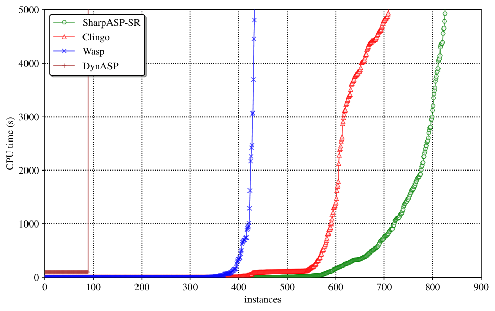
Figure 2: The runtime performance of $\mathsf{sharpASP}$-$\mathcal{SR}$ vis-a-vis other ASP counters.

The cactus plot in Figure 2 illustrates the runtime performance of the four tools, where a point $(x,y)$ indicates that a tool can count $x$ instances within $y$ seconds. The plot shows $\mathsf{sharpASP}$-$\mathcal{SR}$’s clear performance advantage over state-of-the-art answer set counters for disjunctive logic programs.

$|\mathsf{LA}(P)|$	$\sum$	clingo	DynASP	Wasp	$\mathsf{sharpASP}$-$\mathcal{SR}$	clingo +$\mathsf{sharpASP}$-$\mathcal{SR}$
$[1,100]$	399	248	87	165	386	388
$[101,1000]$	519	316	2	142	398	401
$>1000$	207	144	0	125	41	129

Table 3: The performance comparison of $\mathsf{sharpASP}$-$\mathcal{SR}$ (SA) vis-a-vis existing disjunctive answer set counters across instances with varying numbers of loop atoms. The second column ($\sum$) indicates the number of instances within each range of $|\mathsf{LA}(P)|$.

Since clingo and Wasp employ enumeration-based techniques, their performance is inherently constrained by the answer set count. Our analysis revealed that clingo (resp. Wasp) timed out on nearly all instances with approximately $2^{30}$ (resp. $2^{24}$) or more answer sets, while $\mathsf{sharpASP}$-$\mathcal{SR}$ can count instances upto $2^{127}$ answer sets. However, the performance of $\mathsf{sharpASP}$-$\mathcal{SR}$ is primarily influenced by the hardness of the projected model counting, which is related to the cyclicity of the program. The cyclicity of a program is quantified using the measure $|\mathsf{LA}(P)|$.

To analyze $\mathsf{sharpASP}$-$\mathcal{SR}$’s performance relative to $|\mathsf{LA}(P)|$, we compared different ASP counters across varying ranges of loop atoms. The results in the Table 3 indicate that while $\mathsf{sharpASP}$-$\mathcal{SR}$ performs exceptionally well on instances with fewer loop atoms, its performance deteriorates significantly for instances with a higher number of loop atoms (e.g., those with $|\mathsf{LA}(P)|>1000$), leading to a decrease in the solved instances count.

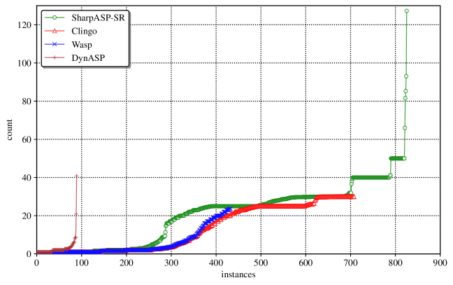
Figure 3: The performance comparison of $\mathsf{sharpASP}$-$\mathcal{SR}$ in terms of the number of answer sets. The $x$ and $y$-axis indicate the number of instances and answer set count (in $2$-base log scale), respectively.

To further analyze the performance of $\mathsf{sharpASP}$-$\mathcal{SR}$, we compare the number of answer sets for each instance solved by different ASP counters. We visually present these comparisons in Figure 3. In the plot, a point $(x,y)$ indicates that a tool can count $x$ instances, where each instance has up to $2^{y}$ answer sets. Since both clingo and Wasp count using enumeration, clingo and Wasp  can handle instances with up to $2^{30}$ and $2^{24}$ answer sets (roughly) respectively, whereas $\mathsf{sharpASP}$-$\mathcal{SR}$ is capable of counting instances having $2^{127}$ answer sets. Due to its use of projected model counting, $\mathsf{sharpASP}$-$\mathcal{SR}$ demonstrates superior scalability on instances with a large number of answer sets.

Further experimental evaluation of $\mathsf{sharpASP}$-$\mathcal{SR}$ is provided in the C.

7 Conclusion

In this paper, we introduced $\mathsf{sharpASP}$-$\mathcal{SR}$, a novel answer set counter based on subtractive reduction. By leveraging an alternative definition of answer sets, $\mathsf{sharpASP}$-$\mathcal{SR}$ achieves significant performance improvements over baseline approaches, owing to its ability to rely on the scalability of state-of-the-art projected model counting techniques. Our experimental results demonstrate the effectiveness and efficiency of our approach across a range of benchmarks.

The use of subtractive reductions for empirical efficiency opens up potential avenues for future work. In particular, an interesting direction would be to categorize problems that can be reduced to #SAT via subtractive methods, which would allow us to utilize existing #SAT model counters.

Appendix

Appendix A An Illustrative Example

Example to illustrate Justification of atoms

Example A.9 (continued).

Consider the following two interpretations over $\and{P}$:

• $M_{1}=\{p_{0},w,q_{0},q_{1}\}$: clearly, $\tau_{M_{1}}=\{p_{0},w,q_{0},q_{1},\neg{p_{1}}\}$. As no proper subset of $M_{1}$ satisfies $P^{M_{1}}$, each atom of $M_{1}$ is justified.

• $M_{2}=\{p_{1},w,q_{0},q_{1}\}$: here, $\tau_{M_{2}}=\{p_{1},w,q_{0},q_{1},\neg{p_{0}}\}$. Note that $\tau_{M_{2}}\models\mathsf{Comp}(P)$. The program $P^{M_{2}}$ includes all rules of $P$ except rule $r_{7}$. There exists an interpretation $\{p_{1},q_{0}\}\subset M_{2}$ such that $\{p_{1},q_{0}\}$ satisfies $P^{M_{2}}$. It indicates that atoms $q_{1}$ and $w$ are not justified in $M_{2}$.

Example to illustrate Lemma 4.2

Example A.10 (continued).

Consider the following two interpretations over $\and{P}$:

• $M_{1}=\{p_{0},w,q_{0},q_{1}\}$: clearly, $\tau_{M_{1}}=\{p_{0},w,q_{0},q_{1},\neg{p_{1}}\}$. Note that $M_{1}\in\mathsf{AS}(P)$, as no strict subset of $M_{1}$ satisfies $P^{M_{1}}$.

• $M_{2}=\{p_{1},w,q_{0},q_{1}\}$: here, $\tau_{M_{2}}=\{p_{1},w,q_{0},q_{1},\neg{p_{0}}\}$. While $\tau_{M_{2}}\models\mathsf{Comp}(P)$, it can be shown that $M_{2}\not\in\mathsf{AS}(P)$. The program $P^{M_{2}}$ includes all rules of $P$ except rule $r_{7}$. There exists an interpretation $\{p_{1},q_{0}\}\subset M_{2}$ such that $\{p_{1},q_{0}\}$ satisfies $P^{M_{2}}$. This means that the atoms $q_{1}$ and $w$ in $M_{2}$ are not justified. Note that both $q_{1}$ and $w$ are loop atoms of program $P$.

Example to illustrate

$\mathsf{Copy}(P)$

Example A.11 (continued).

For the given program $P$, we have $\mathsf{LA}(P)=\{q_{1},w\}$. Therefore, $\mathsf{Copy}(P)$ introduces two fresh copy variables $q_{1}\textprime$ and $w\textprime$, and $\mathsf{Copy}(P)$ consists of the following implications: $\{q_{1}\textprime\longrightarrow q_{1},w\textprime\longrightarrow w,q_{0}\vee q_{1}\textprime,w\textprime\longrightarrow q_{1}\textprime,p_{0}\longrightarrow w\textprime,p_{1}\wedge q_{1}\textprime\longrightarrow w\textprime\}$.

Example to illustrate Lemma 4.4

Example A.12 (continued).

Consider two interpretations $M_{1},M_{2}\subseteq\and{P}$:

• $M_{1}=\{p_{0},w,q_{0},q_{1}\}$, where $\tau_{M_{1}}=\{p_{0},w,q_{0},q_{1},\neg{p_{1}}\}$. Note that $M_{1}\in\mathsf{AS}(P)$ and we can verify that ${\mathsf{Copy}(P)}|_{{\tau_{M_{1}}}}\wedge(\neg{q_{1}\textprime}\vee\neg{w\textprime})$ is UNSAT.

• $M_{2}=\{p_{1},w,q_{0},q_{1}\}$, where $\tau_{M_{2}}=\{p_{1},w,q_{0},q_{1},\neg{p_{0}}\}$. Here, $M_{2}\not\in\mathsf{AS}(P)$. While $\tau_{M_{2}}\models\mathsf{Comp}(P)$, we can see that ${\mathsf{Copy}(P)}|_{{\tau_{M_{2}}}}\wedge(\neg{q_{1}\textprime}\vee\neg{w\textprime})=(\neg{w\textprime}\vee q_{1}\textprime)\wedge(\neg{q_{1}\textprime}\vee w\textprime)\wedge(\neg{w\textprime}\vee\neg{q_{1}\textprime})$ is SAT.

Appendix B Proofs Deferred to the Appendix

See 4.2

Proof B.13.

For notational clarity, let $A$ and $B$ denote the formulas $P^{M}\wedge\bigwedge_{x\in\tau_{M}^{-}}\neg{x}\wedge\bigvee_{x\in\tau_{M}^{+}}\neg{x}$ and $P^{M}\wedge\bigwedge_{x\in\tau_{M}^{-}}\neg{x}\wedge\bigwedge_{x\in\tau_{M}^{+}\wedge x\not\in\mathsf{LA}(P)}x\wedge\bigvee_{x\in\tau_{M}^{+}\wedge x\in\mathsf{LA}(P)}\neg{x}$, respectively.

We use proof by contradiction. Suppose, if possible, $A$ is SAT but $B$ is UNSAT.

Given that $A$ is SAT, we know that some atoms are not justified in $M$ (Proposition 1). Similarly, since $B$ is UNSAT, we know that all loop atoms are justified in $M$ (Proposition 2). Therefore, there must be a non-loop atom, say $x_{1}$, that is not justified in $M$. Since $x_{1}\in M$ and $\tau_{M}\models\mathsf{Comp}(P)$, according to group $3$ implications in the definition of Clark completion, there exists a rule $r_{1}\in P$ such that $\mathsf{Body}(r_{1})\wedge\bigwedge_{x\in\mathsf{Head}(r_{1})\setminus\{x_{1}\}}\neg{x}$ is true under $\tau_{M}$. It follows that there exists an atom $x_{2}\in\mathsf{Body}(r_{1})^{+}$ that is not justified; otherwise, the atom $x_{1}$ would have no other option but be justified. Now, we can repeat the same argument we presented above for $x_{1}$, but in the context of the non-justified atom $x_{2}$ in $M$. By continuing this argument, we obtain a sequence of not justified atoms $\{x_{1},x_{2},\ldots\}$, such that the underlying set is a subset of $M$. There are two possible cases to consider: either (i) the sequence $\{x_{i}\}$ is unbounded, or (ii) for some $i<j$, $x_{i}=x_{j}$. Case (i) contradicts the finiteness of $\and{P}$. Case (ii) implies that some loop atoms are not justified – a contradiction of our premise!

Proof of Lemma 4.3

See 4.3

Proof B.14.

The proof of “part 1”:
Recall that $P^{M}$ can be thought of as a set of implications (see Section 2). First we discuss which implications are left in the subformula $P^{M}\wedge\bigwedge_{x\in\tau_{M}^{-}}\neg{x}\wedge\bigwedge_{x\in\tau_{M}^{+}\wedge x\not\in\mathsf{LA}(P)}x$, following unit propagation.

Note that the subformula $\bigwedge_{x\in\tau_{M}^{-}}\neg{x}\wedge\bigwedge_{x\in\tau_{M}^{+}\wedge x\not\in\mathsf{LA}(P)}x$ includes a unit clause $\neg{x}$, for each atom $x\in\tau_{M}^{-}$ and a unit clause $x$, each atom $x\in\tau_{M}^{+}\cap\mathsf{LA}(P)$. Since $\tau_{M}\models\mathsf{Comp}(P)$, the unit propagation does not result in any empty clause. When the unit propagation reaches the fixed point, all atoms that are assigned to false ($x\in\tau_{M}^{-}$) and non loop atoms that are assigned to true ($x\in\tau_{M}^{+}\wedge x\not\in\mathsf{LA}(P)$) are removed from implications of $P^{M}$. Thus, after reaching the fixed point, each implication is of the form: $\beta\longrightarrow\alpha$, where $\beta$ (antecedent) is either true or a conjunction of loop atoms, and $\alpha$ (consequent) is a disjunction of loop atoms, where those loop atoms are assigned to true in $\tau_{M}$. Note that no implication left such that its consequent ($\alpha$) part is false but the antecedent ($\beta$) part is a conjunction of loop atoms; otherwise, we can say that $\tau_{M}\not\models\mathsf{Comp}(P)$. In summary, after reaching the unit propagation fixed point, the formula $P^{M}\bigwedge_{x\in\tau_{M}^{-}}\neg{x}\wedge\bigwedge_{x\in\tau_{M}^{+}\wedge x\not\in\mathsf{LA}(P)}x$ is left with a set of unit clauses and implications, where the implications consists of only loop atoms that are assigned to true in $\tau_{M}$.

Now we discuss how the implications of ${\mathsf{Copy}(P)}|_{{\tau_{M}}}$ relate to the implications of $P^{M}\wedge\bigwedge_{x\in\tau_{M}^{-}}\neg{x}\wedge\bigwedge_{x\in\tau_{M}^{+}\wedge x\not\in\mathsf{LA}(P)}x$. According to the definition of the copy operation, $\mathsf{Copy}(P)$ introduces a type 2 implication for every rule whose head has at least one loop atom; that is, $\mathsf{Copy}(P)$ introduces a type 2 implication for a rule $r$ if $\mathsf{Head}(r)\cap\mathsf{LA}(P)\neq\emptyset$. Recall that these type 2 implications are similar to the implications introduced and discussed above for $P^{M}$, except that each of the loop atoms (i.e., $x$) of rule $r$ is replaced by its corresponding copy atom (i.e., $x\textprime$). Clearly, no loop atom of $P$ presents in $\mathsf{Copy}(P)$.

Note that the assignment $\tau_{M}$ does not assign any copy variables. Since $\tau_{M}\models\mathsf{Comp}(P)$, no empty clause is introduced in the unit propagation of ${\mathsf{Copy}(P)}|_{{\tau_{M}}}$. If a loop atom $x\in\mathsf{LA}(P)$ is false in $\tau_{M}$, then the corresponding copy atom $x\textprime$ will be unit propagated to false in ${\mathsf{Copy}(P)}|_{{\tau_{M}}}$, due to the type 1 implication. Finally, no type 1 implication left in ${\mathsf{Copy}(P)}|_{{\tau_{M}}}$ after reaching the unit propagation fixed point. Straightforwardly, the formula ${\mathsf{Copy}(P)}|_{{\tau_{M}}}$ is the conjuction of a set of unit clauses and implications, where these implications consist of only copy atoms such that their corresponding loop atoms are assigned to true in $\tau_{M}$.

From the discussion so far, we can say that the implications of $P^{M}\wedge\bigwedge_{x\in\tau_{M}^{-}}\neg{x}\wedge\bigwedge_{x\in\tau_{M}^{+}\wedge x\not\in\mathsf{LA}(P)}x$ left after unit propagation are identical to the implications left from ${\mathsf{Copy}(P)}|_{{\tau_{M}}}$ after unit propagation, except that each loop atom in $P^{M}$ is replaced by their corresponding copy atom in ${\mathsf{Copy}(P)}|_{{\tau_{M}}}$. Clearly, the satisfiability of both formulas ${\mathsf{Copy}(P)}|_{{\tau_{M}}}\wedge\bigvee_{x\in\tau_{M}^{+}\wedge x\in\mathsf{LA}(P)}\neg{x\textprime}$ and $P^{M}\wedge\bigwedge_{x\in\tau_{M}^{-}}\neg{x}\wedge\bigwedge_{x\in\tau_{M}^{+}\wedge x\not\in\mathsf{LA}(P)}x\wedge\bigvee_{x\in\tau_{M}^{+}\wedge x\in\mathsf{LA}(P)}\neg{x}$ depends only on these implications left so far; since the variables of unit clauses are different from the variables of those implications. From the relationship discussed above and following the Proposition 2, the satisfiability checking of ${\mathsf{Copy}(P)}|_{{\tau_{M}}}\wedge\bigvee_{x\in\tau_{M}^{+}\wedge x\in\mathsf{LA}(P)}\neg{x\textprime}$ can be rephrased as to check justification of all loop atoms in the interpretation $\tau_{M}$. Finally we can say that the formula ${\mathsf{Copy}(P)}|_{{\tau_{M}}}\wedge\bigvee_{x\in\tau_{M}^{+}\wedge x\in\mathsf{LA}(P)}\neg{x\textprime}$ is SAT if and only if $P^{M}\wedge\bigwedge_{x\in\tau_{M}^{-}}\neg{x}\wedge\bigwedge_{x\in\tau_{M}^{+}\wedge x\not\in\mathsf{LA}(P)}x\wedge\bigvee_{x\in\tau_{M}^{+}\wedge x\in\mathsf{LA}(P)}\neg{x}$ is SAT (the satisfiability of both formulas have the same meaning).

The proof of “part 2”:
We use the relationship established between the implications in ${\mathsf{Copy}(P)}|_{{\tau_{M}}}$ and implications in $P^{M}$ in the proof of part 1.

proof of “if part”: The proof of “if part” follows Lemma 4.2 — the Lemma 4.2 proves that if some atoms of $M$ are not justified (or $P^{M}\wedge\bigwedge_{x\in\tau_{M}^{-}}\neg{x}\wedge\bigvee_{x\in\tau_{M}^{+}}\neg{x}$ is SAT), then some loop atoms of $M$ are not justified (or ${\mathsf{Copy}(P)}|_{{\tau_{M}}}\wedge\bigvee_{x\in\tau_{M}^{+}\wedge x\in\mathsf{LA}(P)}\neg{x\textprime}$ is SAT). We have already shown that (in part 1) the satisfiability checking of ${\mathsf{Copy}(P)}|_{{\tau_{M}}}\wedge\bigvee_{x\in\tau_{M}^{+}\wedge x\in\mathsf{LA}(P)}\neg{x\textprime}$ can be rephrased as to check justification of all loop atoms in the interpretation $\tau_{M}$. So, the “if part” is proved.

proof of “only if part”: The proof is trivial. If some loop atoms of $M$ are not justified, then some atoms of $M$ are not justified. So, the “only if part” is proved.

Appendix C Further Experimental Analysis

Performance comparison of different ASP counters across different computation problems.

We present the Table 4 showing the number of instances across different benchmark classes solved by different ASP counters. We observe that there are two benchmark classes: preferred extension and diagnosis, where the performance of $\mathsf{sharpASP}$-$\mathcal{SR}$ is surpassed by clingo. Our observations reveal that these instances tend to have a significantly larger number of loop atoms. More specifically, around $66\%$ of Preferred extension instances and $100\%$ of Diagnosis instances contain more than $1000$ loop atoms.

	$\sum$	$\sum^{\geq 1000}$	clingo	DynASP	Wasp	$\mathsf{sharpASP}$-$\mathcal{SR}$
$2$QBF	200	0	179	0	58	181
Strategic	226	0	53	0	0	125
Preferred	217	142	208	2	192	110
PC config	1	1	0	0	0	0
Diagnosis	11	11	11	0	8	6
Random	226	0	80	0	0	213
MTS	244	53	177	87	174	190
			708	89	432	825

Table 4: The performance comparison of different ASP counters across different benchmark classes. The second ($\sum$) and third columns ($\sum^{\geq 1000}$) represents the total number of instances and total number of instances having more that $1000$ loop atoms in each benchmark class, respectively.

Experimentals with Alternative Projected Model Counters ($\#\exists$SAT solvers) and ApproxASP.

We conducted experiments with alternative projected model counters, including D$4$ (Lagniez and Marquis, 2017), GPMC (Suzuki et al., 2017), as well as the approximate answer set counter ApproxASP (Kabir et al., 2022). The results of these experiments, comparing the performance of the alternative counting techniques, are summarized in Table 5. The results reveal that $\mathsf{sharpASP}$-$\mathcal{SR}$ with GANAK outperforms $\mathsf{sharpASP}$-$\mathcal{SR}$ with alternative projected model counters.

	D4	GPMC	ApproxASP
#Solved ($1125$)	697	759	715
PAR$2$	3856	3463	3829

Table 5: The performance comparison of alternative $\#\exists$SAT counting techniques and approximate counter ApproxASP.

Experimentals with $16$ GB Memory Limit

We set the memory limit of $8$ GB, which is consistent with prior works on answer set counting (Kabir et al., 2024; Fichte et al., 2024; Eiter et al., 2021). Additionally, we conducted another set of experiments with a $16$ GB memory limit and the result is summarized in Table 6. The findings indicate a slight increase in the number of solved instances for most ASP counters, with the exception of Wasp. Specifically, the increase in solved instances was clingo ($+10$), DynASP ($+8$), Wasp ($+96$), and $\mathsf{sharpASP}$-$\mathcal{SR}$ remained unchanged.

	clingo	DynASP	Wasp	$\mathsf{sharpASP}$-$\mathcal{SR}$
#Solved ($1125$)	718	97	528	825
PAR$2$	4025	9137	5552	2876

Table 6: The performance of $\mathsf{sharpASP}$-$\mathcal{SR}$ vis-a-vis existing disjunctive answer set counters, with a $16$ GB memory limit.

References

- Alviano et al., (2019) Alviano, M., Amendola, G., Dodaro, C., Leone, N., Maratea, M., and Ricca, F. Evaluation of disjunctive programs in Wasp. In LPNMR 2019, pp. 241–255. Springer.
- Alviano et al., (2015) Alviano, M., Dodaro, C., Leone, N., and Ricca, F. Advances in Wasp. In LPNMR 2015, pp. 40–54. Springer.
- Amendola et al., (2017) Amendola, G., Ricca, F., and Truszczynski, M. Generating hard random boolean formulas and disjunctive logic programs. In IJCAI 2017, pp. 532–538.
- (4) Aziz, R. A., Chu, G., Muise, C., and Stuckey, P. SAT: Projected model counting. In SAT 2015a, pp. 121–137. Springer.
- (5) Aziz, R. A., Chu, G., Muise, C., and Stuckey, P. J. Stable model counting and its application in probabilistic logic programming. In AAAI 2015b.
- Balyo et al., (2017) Balyo, T., Heule, M. J., and Järvisalo, M. SAT competition 2017–solver and benchmark descriptions. pp. 14–15 2017.
- Ben-Eliyahu and Dechter, (1994) Ben-Eliyahu, R. and Dechter, R. Propositional semantics for disjunctive logic programs. Annals of Mathematics and Artificial intelligence, 12:53–87 1994.
- Ben-Eliyahu-Zohary et al., (2017) Ben-Eliyahu-Zohary, R., Angiulli, F., Fassetti, F., and Palopoli, L. Modular construction of minimal models. In LPNMR 2017, pp. 43–48. Springer.
- Bend´ık and Meel, (2021) Bendík, J. and Meel, K. S. Counting minimal unsatisfiable subsets. In CAV 2021, pp. 313–336. Springer.
- Capelli et al., (2024) Capelli, F., Lagniez, J.-M., Plank, A., and Seidl, M. A top-down tree model counter for quantified boolean formulas. IJCAI 2024.
- Clark, (1978) Clark, K. L. Negation as failure. Logic and data bases, pp. 293–322 1978.
- Durand et al., (2005) Durand, A., Hermann, M., and Kolaitis, P. G. Subtractive reductions and complete problems for counting complexity classes. Theoretical Computer Science, 340(3):496–513 2005.
- Egly et al., (2000) Egly, U., Eiter, T., Tompits, H., and Woltran, S. Solving advanced reasoning tasks using quantified boolean formulas. In AAAI/IAAI 2000, pp. 417–422.
- Eiter et al., (2004) Eiter, T., Fink, M., Tompits, H., and Woltran, S. On eliminating disjunctions in stable logic programming. KR, 4:447–458 2004.
- Eiter and Gottlob, (1995) Eiter, T. and Gottlob, G. On the computational cost of disjunctive logic programming: Propositional case. Annals of Mathematics and Artificial Intelligence, 15:289–323 1995.
- Eiter et al., (2021) Eiter, T., Hecher, M., and Kiesel, R. Treewidth-aware cycle breaking for algebraic answer set counting. In KR 2021, pp. 269–279.
- Eiter et al., (2024) Eiter, T., Hecher, M., and Kiesel, R. aspmc: New frontiers of algebraic answer set counting. Artificial Intelligence, 330:104109 2024.
- Fages, (1994) Fages, F. Consistency of Clark’s completion and existence of stable models. Journal of Methods of logic in computer science, 1(1):51–60 1994.
- Fandinno and Schulz, (2019) Fandinno, J. and Schulz, C. Answering the “why” in answer set programming–a survey of explanation approaches. TPLP, 19(2):114–203 2019.
- Fichte et al., (2024) Fichte, J. K., Gaggl, S. A., Hecher, M., and Rusovac, D. IASCAR: Incremental answer set counting by anytime refinement. TPLP, 24(3):505–532 2024.
- Fichte et al., (2022) Fichte, J. K., Gaggl, S. A., and Rusovac, D. Rushing and strolling among answer sets–navigation made easy. In AAAI 2022, volume 36, pp. 5651–5659.
- Fichte and Hecher, (2019) Fichte, J. K. and Hecher, M. Treewidth and counting projected answer sets. In LPNMR 2019, pp. 105–119. Springer.
- Fichte et al., (2017) Fichte, J. K., Hecher, M., Morak, M., and Woltran, S. Answer set solving with bounded treewidth revisited. In LPNMR 2017, pp. 132–145.
- Fichte and Szeider, (2015) Fichte, J. K. and Szeider, S. Backdoors to normality for disjunctive logic programs. TOCL, 17(1):1–23 2015.
- Gaggl et al., (2015) Gaggl, S. A., Manthey, N., Ronca, A., Wallner, J. P., and Woltran, S. Improved answer set programming encodings for abstract argumentation. TPLP, 15(4-5):434–448 2015.
- Gebser et al., (2012) Gebser, M., Kaufmann, B., and Schaub, T. Conflict-driven answer set solving: From theory to practice. Artificial Intelligence, 187:52–89 2012.
- Gebser et al., (2020) Gebser, M., Maratea, M., and Ricca, F. The seventh answer set programming competition: Design and results. TPLP, 20(2):176–204 2020.
- Gebser et al., (2008) Gebser, M., Schaub, T., Thiele, S., Usadel, B., and Veber, P. Detecting inconsistencies in large biological networks with answer set programming. In ICLP 2008, pp. 130–144. Springer.
- Gelfond and Lifschitz, (1988) Gelfond, M. and Lifschitz, V. The stable model semantics for logic programming. In ICLP/SLP 1988, volume 88, pp. 1070–1080.
- Gelfond and Lifschitz, (1991) Gelfond, M. and Lifschitz, V. Classical negation in logic programs and disjunctive databases. New generation computing, 9:365–385 1991.
- Hecher, (2022) Hecher, M. Treewidth-aware reductions of normal ASP to SAT–is normal ASP harder than SAT after all? Artificial Intelligence, 304:103651 2022.
- Hecher and Kiesel, (2023) Hecher, M. and Kiesel, R. The impact of structure in answer set counting: fighting cycles and its limits. In KR 2023, pp. 344–354.
- Hemaspaandra and Vollmer, (1995) Hemaspaandra, L. A. and Vollmer, H. The satanic notations: counting classes beyond P and other definitional adventures. ACM SIGACT News, 26(1):2–13 1995.
- Janhunen, (2006) Janhunen, T. Some (in) translatability results for normal logic programs and propositional theories. Journal of Applied Non-Classical Logics, 16(1-2):35–86 2006.
- Janhunen and Niemelä, (2011) Janhunen, T. and Niemelä, I. 2011. Compact Translations of Non-disjunctive Answer Set Programs to Propositional Clauses, pp. 111–130.
- Janhunen et al., (2006) Janhunen, T., Niemelä, I., Seipel, D., Simons, P., and You, J.-H. Unfolding partiality and disjunctions in stable model semantics. TOCL, 7(1):1–37 2006.
- Ji et al., (2016) Ji, J., Wan, H., Wang, K., Wang, Z., Zhang, C., and Xu, J. Eliminating disjunctions in answer set programming by restricted unfolding. In IJCAI 2016, pp. 1130–1137.
- Kabir, (2024) Kabir, M. Minimal model counting via knowledge compilation. arXiv preprint arXiv:2409.10170 2024.
- Kabir et al., (2024) Kabir, M., Chakraborty, S., and Meel, K. S. Exact ASP counting with compact encodings. In AAAI 2024, volume 38, pp. 10571–10580.
- Kabir et al., (2022) Kabir, M., Everardo, F. O., Shukla, A. K., Hecher, M., Fichte, J. K., and Meel, K. S. ApproxASP–a scalable approximate answer set counter. In AAAI 2022, pp. 5755–5764.
- Kabir and Meel, (2023) Kabir, M. and Meel, K. S. A fast and accurate ASP counting based network reliability estimator. In LPAR 2023, pp. 270–287.
- Kabir and Meel, (2024) Kabir, M. and Meel, K. S. On lower bounding minimal model count. TPLP, 24(4):586–605 2024.
- Kabir and Meel, (2025) Kabir, M. and Meel, K. S. An ASP-based framework for MUSes. arXiv preprint arXiv:2507.03929 2025.
- Kabir et al., (2025) Kabir, M., Trinh, V.-G., Pastva, S., and Meel, K. S. Scalable counting of minimal trap spaces and fixed points in boolean networks. arXiv preprint arXiv:2506.06013 2025.
- Kanchanasut and Stuckey, (1992) Kanchanasut, K. and Stuckey, P. J. Transforming normal logic programs to constraint logic programs. TCS, 105(1):27–56 1992.
- Lagniez and Marquis, (2017) Lagniez, J.-M. and Marquis, P. An improved decision-DNNF compiler. In IJCAI 2017, volume 17, pp. 667–673.
- Lagniez and Marquis, (2019) Lagniez, J.-M. and Marquis, P. A recursive algorithm for projected model counting. In AAAI 2019, volume 33, pp. 1536–1543.
- Lee and Lifschitz, (2003) Lee, J. and Lifschitz, V. Loop formulas for disjunctive logic programs. In ICLP 2003, pp. 451–465. Springer.
- Lee et al., (2017) Lee, J., Talsania, S., and Wang, Y. Computing LPMLN using ASP and MLN solvers. Theory and Practice of Logic Programming, 17(5-6):942–960 2017.
- Leone and Ricca, (2015) Leone, N. and Ricca, F. Answer set programming: A tour from the basics to advanced development tools and industrial applications. In Reasoning web international summer school 2015, pp. 308–326. Springer.
- Lierler, (2005) Lierler, Y. Cmodels–SAT-based disjunctive answer set solver. In LPNMR 2005, pp. 447–451. Springer.
- Lifschitz, (2010) Lifschitz, V. Thirteen definitions of a stable model. Fields of logic and computation, pp. 488–503 2010.
- Lifschitz and Razborov, (2006) Lifschitz, V. and Razborov, A. Why are there so many loop formulas? TOCL, 7(2):261–268 2006.
- Marek and Truszczyński, (1999) Marek, V. W. and Truszczyński, M. Stable models and an alternative logic programming paradigm. In The Logic Programming Paradigm 1999, pp. 375–398. Springer.
- Marek and Truszczyński, (1991) Marek, W. and Truszczyński, M. Autoepistemic logic. Journal of the ACM (JACM), 38(3):587–618 1991.
- Nogueira et al., (2001) Nogueira, M., Balduccini, M., Gelfond, M., Watson, R., and Barry, M. An A-Prolog decision support system for the space shuttle. In PADL 2001, pp. 169–183. Springer.
- Pontelli et al., (2009) Pontelli, E., Son, T. C., and Elkhatib, O. Justifications for logic programs under answer set semantics. TPLP, 9(1):1–56 2009.
- Rusovac et al., (2024) Rusovac, D., Hecher, M., Gebser, M., Gaggl, S. A., and Fichte, J. K. Navigating and querying answer sets: how hard is it really and why? In KR 2024, volume 21, pp. 642–653.
- Sharma et al., (2019) Sharma, S., Roy, S., Soos, M., and Meel, K. S. GANAK: A scalable probabilistic exact model counter. In IJCAI 2019, volume 19, pp. 1169–1176.
- Shukla et al., (2022) Shukla, A., Möhle, S., Kauers, M., and Seidl, M. Outercount: A first-level solution-counter for quantified boolean formulas. In CICM 2022, pp. 272–284. Springer.
- Suzuki et al., (2017) Suzuki, R., Hashimoto, K., and Sakai, M. 2017. Improvement of projected model-counting solver with component decomposition using sat solving in components. Technical report, JSAI.
- Trinh et al., (2024) Trinh, G., Benhamou, B., Pastva, S., and Soliman, S. Scalable enumeration of trap spaces in boolean networks via answer set programming. In AAAI 2024, volume 38, pp. 10714–10722.
- Valiant, (1979) Valiant, L. G. The complexity of enumeration and reliability problems. SIAM Journal on Computing, 8(3):410–421 1979.
- Zhou, (2014) Zhou, Y. From disjunctive to normal logic programs via unfolding and shifting. In ECAI 2014 2014, pp. 1139–1140. IOS Press.