State-based approach to the numerical solution of Dirichlet boundary optimal control problems for the Laplace equation

Abstract

We investigate the Dirichlet boundary control of the Laplace equation, considering the control in $H^{1/2}(\partial\Omega)$, which is the natural space for Dirichlet data when the state belongs to $H^{1}(\Omega)$. The cost of the control is measured in the $H^{1/2}(\partial\Omega)$ norm that also plays the role of the regularization term. We discuss regularization and finite element error estimates enabling us to derive an optimal relation between the finite element mesh size $h$ and the regularization parameter $\varrho$, balancing the energy cost for the control and the accuracy of the approximation of the desired state. This relationship is also crucial in designing efficient solvers. We also discuss additional box constraints imposed on the control and the state. Our theoretical findings are complemented by numerical examples, including one example with box constraints.

Keywords: Dirichlet boundary control problems, Laplace equation, finite element discretization, error estimates, solution methods.

2020 MSC: 49J20, 49K20, 65K10, 65N30, 65N22

1 Introduction

We consider the boundary optimal control problem to minimize the cost functional

$${\mathcal{J}}(y_{\varrho},u_{\varrho})=\frac{1}{2}\,\|y_{\varrho}-\overline{y}\|^{2}_{L^{2}(\Omega)}+\frac{1}{2}\,\varrho\,\|u_{\varrho}\|^{2}_{U}$$ (1.1)

subject to the Dirichlet boundary value problem for the Laplace equation,

$$-\Delta y_{\varrho}=0\quad\mbox{in}\;\Omega,\quad y_{\varrho}=u_{\varrho}\quad\mbox{on}\;\Gamma=\partial\Omega.$$ (1.2)

Here, $\Omega\subset{\mathbb{R}}^{d}$, $d=2,3$, is a bounded domain with Lipschitz boundary $\Gamma=\partial\Omega$, $\overline{y}\in L^{2}(\Omega)$ is a given target, $\varrho\in(0,1]$ is some regularization or cost parameter which the solution depends on, and $U$ is the control space.

The mathematical analysis of abstract optimal control problems goes back to the pioneering work of Lions [32], see also the more recent text books [23, 45]. Dirichlet boundary control problems play an important role in the context of computational fluid mechanics, see, e.g., [17, 20, 22]; for related work for parabolic evolution equations, see, e.g., [3, 26, 30, 31]. In [26], the authors give an overview on different approaches to handle Dirichlet boundary control problems by considering different control spaces, including $U=L^{2}(\Gamma)$, $U=H^{1/2}(\Gamma)$, and $U=H^{1}(\Gamma)$. The latter was used to avoid difficulties with implementing the $H^{1/2}$-norm which, at first glance, seems to be more involved to realize than the $L^{2}$-norm. In fact, the most standard choice in Dirichlet boundary control problems is to consider $U=L^{2}(\Gamma)$ where the Dirichlet boundary value problem (1.2) is formulated in a very weak sense [8], see, e.g., [2, 12, 13, 16, 34]. However, when considering the Dirichlet boundary value problem (1.2), $U=H^{1/2}(\Gamma)$ appears as a natural choice [7]. In [37], we have considered a finite element formulation for the solution of Dirichlet boundary control problems when using the regularization norm induced by the Steklov–Poincaré operator $S:H^{1/2}(\Gamma)\to H^{-1/2}(\Gamma)$, see also [14]. Since the Steklov–Poincaré operator computes the normal derivative of the harmonic extension of a given Dirichlet datum, this norm representation is equal to the Dirichlet norm as used in the variational formulation of Neumann boundary value problems for the Laplacian. In this case, the abstract theory as presented recently in [29] is applicable, as we will see in this paper. In particular, if the target $\overline{y}$ itself is harmonic, we can derive related regularization error estimates which depend on the Sobolev regularity of the target $\overline{y}$, and on the smoothness of the domain. In the more general situation when the target $\overline{y}$ is not harmonic, we determine the best approximation of the target in the space of harmonic functions. For the finite element discretization of the gradient equation in the space of harmonic functions, we apply a non-conforming mixed approach, for which we prove related finite element error estimates and establish optimal relations between the regularization parameter $\varrho$ and the finite element mesh size $h$. This optimal choice also enables an efficient iterative solution of the discrete system which is related to the first biharmonic boundary value problem. Hence we can apply well known preconditioning techniques, e.g., [9, 19, 27, 38]. However, the relation of Dirichlet boundary control problems with the first biharmonic boundary value problem has some serious implications when considering domains with a piecewise smooth boundary: In the case of the control space $U=H^{1/2}(\Gamma)$, we have to adapt the optimal choice of the regularization parameter $\varrho$ as a function of the finite element mesh size $h$ by some additional logarithmic terms. When using $U=L^{2}(\Gamma)$, we even have a reduced regularity of the optimal control which, in the case of a two-dimensional domain with piecewise smooth boundary, is zero in all corner points, see [34, Remark 1] and [37, Figure 3].

The rest of the paper is organized as follows. Section 2 starts with the setting of the Dirichlet boundary optimal control problem for the Laplace equation with energy regularization. Furthermore, we derive estimates of the deviation of the state $y_{\varrho}$ from the given desired state $\overline{y}$ in the $L^{2}$ norm as well as estimates of the energy cost of the control in terms of $\varrho$ and in dependence of the regularity of the desired state $\overline{y}$ and the computational domain $\Omega$. The finite element discretization together with the corresponding discretization error analysis is performed in Section 3. It turns out that the cost parameter $\varrho$ must be balanced with the mesh size $h$ in order to obtain asymptotically optimal estimates under minimal energy costs. Section 4 is devoted to the efficient solution of the resulting mixed finite element scheme. In Section 5, we briefly show that control and state constraints can easily be incorporated into our framework. The numerical results presented in Section 6 illustrate the theoretical findings quantitatively. We tested our approach for 2D and 3D benchmark problems with different features. Finally, we draw some conclusions, and give an outlook on further topics.

2 Boundary control of the Laplace equation

In the case of energy regularization with the control space $U=H^{1/2}(\Gamma)$, we consider the boundary optimal control problem to minimize the cost functional

$${\mathcal{J}}(y_{\varrho},u_{\varrho})=\frac{1}{2}\,\|y_{\varrho}-\overline{y}\|^{2}_{L^{2}(\Omega)}+\frac{1}{2}\,\varrho\,|u_{\varrho}|^{2}_{H^{1/2}(\Gamma)}$$ (2.1)

subject to the Dirichlet boundary value problem (1.2). Hence, we define the state space

$$Y:=\Big{\{}y\in H^{1}(\Omega):\langle\nabla y,\nabla v\rangle_{L^{2}(\Omega)}=0\;\,\forall v\in H^{1}_{0}(\Omega)\Big{\}}$$

of all harmonic functions. The state to control map is the interior Dirichlet trace operator $\gamma_{0}^{int}:Y\to H^{1/2}(\Gamma)$ which is an isomorphism. Once the optimal state $y_{\varrho}\in Y$ is known, the related optimal control $u_{\varrho}=\gamma_{0}^{int}y_{\varrho}$ is nothing but the trace of $y_{\varrho}$ on $\Gamma$. The semi-norm in $H^{1/2}(\Gamma)$ is induced by the Steklov–Poincaré operator, e.g., [1, 40, 44], ${\mathcal{S}}:H^{1/2}(\Gamma)\to H^{-1/2}(\Gamma)$, defined as

$$|u_{\varrho}|^{2}_{H^{1/2}(\Gamma)}=\langle{\mathcal{S}}u_{\varrho},u_{\varrho}\rangle_{\Gamma}=\int_{\Gamma}\frac{\partial}{\partial n_{x}}y_{\varrho}(x)\,u_{\varrho}(x)\,dx=\int_{\Omega}|\nabla y_{\varrho}(x)|^{2}\,dx,$$

where $y_{\varrho}\in Y$ is the harmonic extension of $u_{\varrho}\in H^{1/2}(\Gamma)$. Instead of (2.1), we now consider the reduced state-based cost functional

$$\widetilde{\mathcal{J}}(y_{\varrho})=\frac{1}{2}\,\|y_{\varrho}-\overline{y}\|^{2}_{L^{2}(\Omega)}+\frac{1}{2}\,\varrho\,\|\nabla y_{\varrho}\|^{2}_{L^{2}(\Omega)}\quad\mbox{for}\;y_{\varrho}\in Y.$$ (2.2)

The minimizer of the reduced cost functional (2.2) is given as the unique solution $y_{\varrho}\in Y$ of the gradient equation such that

$$a(y_{\varrho},y):=\int_{\Omega}y_{\varrho}(x)\,y(x)\,dx+\varrho\int_{\Omega}\nabla y_{\varrho}(x)\cdot\nabla y(x)\,dx\,=\,\int_{\Omega}\overline{y}(x)\,y(x)\,dx$$ (2.3)

is satisfied for all $y\in Y$. When introducing the weighted norm

$$\|y\|_{Y}:=\left(\int_{\Omega}[y(x)]^{2}\,dx+\varrho\int_{\Omega}|\nabla y(x)|^{2}\,dx\right)^{1/2},$$

we immediately conclude ellipticity and boundedness of the bilinear form $a(\cdot,\cdot)$,

$$a(y,y)=\|y\|^{2}_{Y},\quad|a(y,v)|\leq\|y\|_{Y}\|v\|_{Y}\quad\mbox{for all}\;y,v\in Y.$$ (2.4)

The variational formulation (2.3) corresponds to the abstract setting as considered in [29, Lemma 1]. Hence, we have the following results: For $\overline{y}\in L^{2}(\Omega)$, there holds

$$\|y_{\varrho}-\overline{y}\|_{L^{2}(\Omega)}\leq\|\overline{y}\|_{L^{2}(\Omega)},$$ (2.5)

as well as

$$\|y_{\varrho}\|_{L^{2}(\Omega)}\leq\|\overline{y}\|_{L^{2}(\Omega)},\quad\|\nabla y_{\varrho}\|_{L^{2}(\Omega)}\leq\varrho^{-1/2}\,\|\overline{y}\|_{L^{2}(\Omega)}.$$ (2.6)

For $\overline{y}\in Y$, we have

$$\|y_{\varrho}-\overline{y}\|_{L^{2}(\Omega)}\leq\varrho^{1/2}\,\|\nabla\overline{y}\|_{L^{2}(\Omega)},\quad\|\nabla(y_{\varrho}-\overline{y})\|_{L^{2}(\Omega)}\leq\|\nabla\overline{y}\|_{L^{2}(\Omega)},$$ (2.7)

as well as

$$\|\nabla y_{\varrho}\|_{L^{2}(\Omega)}\leq\|\nabla\overline{y}\|_{L^{2}(\Omega)}.$$ (2.8)

While the regularization error estimates (2.5)–(2.8) hold for Lipschitz domains $\Omega$, for more regular targets $\overline{y}$ we need to formulate additional assumptions on $\Omega$:

Lemma 1.

Let $y_{\varrho}\in Y$ be the unique solution of the variational formulation (2.3). Assume that $\Omega\subset{\mathbb{R}}^{n}$, $n=2,3$, has a smooth boundary $\Gamma$, and $\overline{y}\in Y\cap H^{2}(\Omega)$. Then,

$$\|y_{\varrho}-\overline{y}\|_{L^{2}(\Omega)}\leq c\,\varrho\,\|\overline{y}\|_{H^{2}(\Omega)},\quad\|\nabla(y_{\varrho}-\overline{y})\|_{L^{2}(\Omega)}\leq c\,\varrho^{1/2}\,\|\overline{y}\|_{H^{2}(\Omega)}.$$ (2.9)

Proof.

When considering (2.3) for $y=y_{\varrho}-\overline{y}\in Y$, this gives

$$\|y_{\varrho}-\overline{y}\|^{2}_{L^{2}(\Omega)}+\varrho\,\|\nabla(y_{\varrho}-\overline{y})\|^{2}_{L^{2}(\Omega)}=\varrho\,\langle\nabla\overline{y},\nabla(\overline{y}-y_{\varrho})\rangle_{L^{2}(\Omega)}.$$ (2.10)

Now, using integration by parts, duality, and the trace theorem, we obtain, since $\overline{y}\in Y$ is assumed to be harmonic,

$$\langle\nabla\overline{y},\nabla(\overline{y}-y_{\varrho})\rangle_{L^{2}(\Omega)} = \langle\partial_{n}\overline{y},\overline{y}-y_{\varrho}\rangle_{L^{2}(\Gamma)}$$

$$\hskip-85.35826pt\leq\,\|\partial_{n}\overline{y}\|_{H^{1/2}(\Gamma)}\|\overline{y}-y_{\varrho}\|_{H^{-1/2}(\Gamma)}\,\leq\,c\,\|\overline{y}\|_{H^{2}(\Omega)}\|\overline{y}-y_{\varrho}\|_{H^{-1/2}(\Gamma)}.$$

It remains to consider

$$\|\overline{y}-y_{\varrho}\|_{H^{-1/2}(\Gamma)}=\sup\limits_{0\neq\varphi\in H^{1/2}(\Gamma)}\frac{\langle\overline{y}-y_{\varrho},\varphi\rangle_{\Gamma}}{\|\varphi\|_{H^{1/2}(\Gamma)}},$$

where $\langle\cdot,\cdot\rangle_{\Gamma}$ is the duality pairing as extension of the inner product in $L^{2}(\Gamma)$. For any $\varphi\in H^{1/2}(\Gamma)$ we determine $\psi_{\varphi}\in H^{2}(\Omega)$ as weak solution of the first boundary value problem for the biharmonic equation,

$$\Delta^{2}\psi_{\varphi}=0\quad\mbox{in}\;\Omega,\quad\psi_{\varphi}=0,\quad\partial_{n}\psi_{\varphi}=\varphi\quad\mbox{on}\;\Gamma.$$ (2.11)

With this we can compute, using Green’s formula, recall $\overline{y}-y_{\varrho}\in Y$ being harmonic,

$$\langle\overline{y}-y_{\varrho},\varphi\rangle_{\Gamma} = \int_{\Gamma}[\overline{y}-y_{\varrho}]\,\partial_{n}\psi_{\varphi}\,ds_{x}$$

$$\hskip-56.9055pt=\,\int_{\Omega}\nabla\psi_{\varphi}\cdot\nabla[\overline{y}-y_{\varrho}]\,dx+\int_{\Omega}\Delta\psi_{\varphi}\,[\overline{y}-y_{\varrho}]\,dx$$

$$\hskip-56.9055pt=\,\int_{\Gamma}\frac{\partial}{\partial n_{x}}[\overline{y}-y_{\varrho}]\,\psi_{\varphi}\,ds_{x}+\int_{\Omega}[-\Delta(\overline{y}-y_{\varrho})]\,\psi_{\varphi}\,dx+\int_{\Omega}\Delta\psi_{\varphi}\,[\overline{y}-y_{\varrho}]\,dx$$

$$\hskip-56.9055pt=\,\int_{\Omega}\Delta\psi_{\varphi}\,[\overline{y}-y_{\varrho}]\,dx\,\leq\,\|\Delta\psi_{\varphi}\|_{L^{2}(\Omega)}\|\overline{y}-y_{\varrho}\|_{L^{2}(\Omega)}.$$

Now, using the regularity for the solution $\psi_{\varphi}$ of the first boundary value problem for the biharmonic equation, e.g., [19, Subsection 2.4],

$$\|\Delta\psi\|_{L^{2}(\Omega)}\leq\|\psi\|_{H^{2}(\Omega)}\leq c\,\|\partial_{n}\psi\|_{H^{1/2}(\Gamma)}=c\,\|\varphi\|_{H^{1/2}(\Gamma)},$$

we finally conclude

$$\|\overline{y}-y_{\varrho}\|_{H^{-1/2}(\Gamma)}\leq c\,\|\overline{y}-y_{\varrho}\|_{L^{2}(\Omega)}.$$

Hence, we obtain

$$\|y_{\varrho}-\overline{y}\|^{2}_{L^{2}(\Omega)}+\varrho\,\|\nabla(y_{\varrho}-\overline{y})\|^{2}_{L^{2}(\Omega)}\,\leq\,c\,\varrho\,\|\overline{y}\|_{H^{2}(\Omega)}\|\overline{y}-y_{\varrho}\|_{L^{2}(\Omega)},$$

and the regularization error estimates (2.9) follow. ∎

When the boundary $\Gamma$ is not sufficiently smooth, the normal derivative $\partial_{n}\psi$ even for smooth functions $\psi$ becomes discontinuous, and the proof of Lemma 1 is not valid anymore, i.e., the first boundary value problem for the biharmonic equation (2.11) is not well defined. Therefore, we now consider the case of a piecewise smooth boundary

$$\Gamma=\bigcup\limits_{j=1}^{J}\overline{\Gamma}_{j},\quad\Gamma_{i}\cap\Gamma_{j}=\emptyset\quad\mbox{for}\;j\neq i,$$ (2.12)

and we define the local Sobolev spaces, e.g., [35], $H^{1/2}(\Gamma_{j})$, $\widetilde{H}^{1/2}(\Gamma_{j})=H^{1/2}_{00}(\Gamma_{j})$, with their respective dual spaces $\widetilde{H}^{-1/2}(\Gamma_{j})=[H^{1/2}(\Gamma_{j})]^{*}$, $H^{-1/2}(\Gamma_{j})=[\widetilde{H}^{1/2}(\Gamma_{j})]^{*}$. At this time, we will restrict to the case where $\Omega\subset\mathbb{R}^{2}$.

Lemma 2.

Let $y_{\varrho}\in Y$ be the unique solution of the variational formulation (2.3). Assume that $\Omega\subset{\mathbb{R}}^{2}$ is convex with a piecewise smooth boundary $\Gamma$ as given in (2.12), and assume $\overline{y}\in Y\cap H^{2}(\Omega)$. Then,

$$\|y_{\varrho}-\overline{y}\|_{L^{2}(\Omega)}\leq c\,\varrho\,(1+|\log\varrho|)\,\|\overline{y}\|_{H^{2}(\Omega)},$$ (2.13)

and

$$\|\nabla(y_{\varrho}-\overline{y})\|_{L^{2}(\Omega)}\leq c\,\varrho^{1/2}\,(1+|\log\varrho|)\,\|\overline{y}\|_{H^{2}(\Omega)}.$$ (2.14)

Proof.

We first proceed as in the proof of Lemma 1, i.e., we have (2.10). But now we have to consider

$$\langle\nabla\overline{y},\nabla(\overline{y}-y_{\varrho})\rangle_{L^{2}(\Omega)} = \langle\partial_{n}\overline{y},\overline{y}-y_{\varrho}\rangle_{L^{2}(\Gamma)}\,=\,\sum\limits_{j=1}^{J}\langle\partial_{n}\overline{y},\overline{y}-y_{\varrho}\rangle_{L^{2}(\Gamma_{j})}$$

$$\leq \sum\limits_{j=1}^{J}\|\partial_{n}\overline{y}\|_{H^{1/2}(\Gamma_{j})}\|\overline{y}-y_{\varrho}\|_{\widetilde{H}^{-1/2}(\Gamma_{j})}$$

$$\leq \left(\sum\limits_{j=1}^{J}\|\partial_{n}\overline{y}\|^{2}_{H^{1/2}(\Gamma_{j})}\right)^{1/2}\left(\sum\limits_{j=1}^{J}\|\overline{y}-y_{\varrho}\|^{2}_{\widetilde{H}^{-1/2}(\Gamma_{j})}\right)^{1/2}$$

$$\leq c\,\|\overline{y}\|_{H^{2}(\Omega)}\left(\sum\limits_{j=1}^{J}\|\overline{y}-y_{\varrho}\|^{2}_{\widetilde{H}^{-1/2}(\Gamma_{j})}\right)^{1/2}\,.$$

In order to proceed as in the proof of Lemma 1, we need to replace the local norms $\|\overline{y}-y_{\varrho}\|_{\widetilde{H}^{-1/2}(\Gamma_{j})}$ by $\|\overline{y}-y_{\varrho}\|_{H^{-1/2}(\Gamma_{j})}$. With respect to each $\Gamma_{j}$, we define local finite element spaces $V_{j}:=S_{\eta}^{1}(\Gamma_{j})\cap\widetilde{H}^{1/2}(\Gamma_{j})$ with mesh size $\eta$ of piecewise linear continuous basis functions which are zero at the end points of $\Gamma_{j}$, and $W_{j}:=\widetilde{S}_{\eta}^{1}(\Gamma)$ is the space of piecewise linear functions which are constant at those elements touching an end point of $\Gamma_{j}$, such that $\mbox{dim}\,V_{j}=\mbox{dim}\,W_{j}$. Then we define the generalized $L^{2}$ projection $\widetilde{Q}_{j}(\overline{y}-y_{\varrho})\in W_{j}$ as unique solution of the variational formulation

$$\langle\widetilde{Q}_{j}(\overline{y}-y_{\varrho}),\phi_{j}\rangle_{L^{2}(\Gamma_{j})}=\langle\overline{y}-y_{\varrho},\phi_{j}\rangle_{L^{2}(\Gamma_{j})}\quad\mbox{for all}\;\phi_{j}\in V_{j}.$$

With this we can write, using standard approximation error estimates, e.g., [42, 43], and the trace theorem,

$$\|\overline{y}-y_{\varrho}\|_{\widetilde{H}^{-1/2}(\Gamma_{j})} \leq \|(I-\widetilde{Q}_{j})(\overline{y}-y_{\varrho})\|_{\widetilde{H}^{-1/2}(\Gamma_{j})}+\|\widetilde{Q}_{j}(\overline{y}-y_{\varrho})\|_{\widetilde{H}^{-1/2}(\Gamma_{j})}$$

$$\leq c\,\eta\,|\overline{y}-y_{\varrho}|_{H^{1/2}(\Gamma_{j})}+\|\widetilde{Q}_{j}(\overline{y}-y_{\varrho})\|_{\widetilde{H}^{-1/2}(\Gamma_{j})}$$

$$\leq c\,\eta\,\|\nabla(\overline{y}-y_{\varrho})\|_{L^{2}(\Omega)}+\|\widetilde{Q}_{j}(\overline{y}-y_{\varrho})\|_{\widetilde{H}^{-1/2}(\Gamma_{j})}.$$

It remains to consider

$$\|\widetilde{Q}_{j}(\overline{y}-y_{\varrho})\|_{\widetilde{H}^{-1/2}(\Gamma_{j})}=\sup\limits_{0\neq\varphi\in H^{1/2}(\Gamma_{j})}\frac{\langle\widetilde{Q}_{j}(\overline{y}-y_{\varrho}),\varphi\rangle_{\Gamma_{j}}}{\|\varphi\|_{H^{1/2}(\Gamma_{j})}}\,.$$

Let $\widetilde{Q}_{j}^{*}\varphi\in V_{j}$ be the unique solution of the variational formulation

$$\langle\widetilde{Q}_{j}^{*}\varphi,\psi_{j}\rangle_{L^{2}(\Gamma_{j})}=\langle\varphi,\psi_{j}\rangle_{L^{2}(\Gamma_{j})}\quad\mbox{for all}\;\psi_{j}\in W_{j},$$

and we have

$$\langle\widetilde{Q}_{j}(\overline{y}-y_{\varrho}),\varphi\rangle_{\Gamma_{j}}=\langle\widetilde{Q}_{j}(\overline{y}-y_{\varrho}),\widetilde{Q}_{j}^{*}\varphi\rangle_{L^{2}(\Gamma_{j})}=\langle\overline{y}-y_{\varrho},\widetilde{Q}_{j}^{*}\varphi\rangle_{L^{2}(\Gamma_{j})}.$$

With the stability estimate [42, 43]

$$\|\widetilde{Q}_{j}^{*}\varphi\|_{H^{1/2}(\Gamma_{j})}\leq c\,\|\varphi\|_{H^{1/2}(\Gamma_{j})},$$

and using, since $\widetilde{Q}_{j}^{*}\varphi\in V_{j}\subset\widetilde{H}^{1/2}(\Gamma)$, the estimate [36, Theorem 4.1]

$$\|\widetilde{Q}_{j}^{*}\varphi\|_{\widetilde{H}^{1/2}(\Gamma_{j})}\leq c\,(1+|\log\eta|)\,\|\widetilde{Q}_{j}^{*}\varphi\|_{H^{1/2}(\Gamma_{j})},$$ (2.15)

we further conclude

$$\frac{c}{1+|\log\eta|}\,\|\widetilde{Q}_{j}(\overline{y}-y_{\varrho})\|_{\widetilde{H}^{-1/2}(\Gamma_{j})} \leq \sup\limits_{0\neq\varphi\in H^{1/2}(\Gamma_{j})}\frac{\langle\overline{y}-y_{\varrho},\widetilde{Q}_{j}^{*}\varphi\rangle_{\Gamma_{j}}}{\|\widetilde{Q}_{j}^{*}\varphi\|_{\widetilde{H}^{1/2}(\Gamma_{j})}}$$

$$\leq \|\overline{y}-y_{\varrho}\|_{H^{-1/2}(\Gamma_{j})}\,.$$

Hence we can proceed as in the proof of Lemma 1, i.e., we consider the first boundary value problem for the biharmonic equation (2.11) for functions $\varphi\in H^{1/2}(\Gamma)$ which are zero in all corner points. Then, all arguments as used in the proof of Lemma 1 remain valid, see [46]. From (2.10) we therefore conclude

$$\|y_{\varrho}-\overline{y}\|^{2}_{L^{2}(\Omega)}+\varrho\,\|\nabla(y_{\varrho}-\overline{y})\|^{2}_{L^{2}(\Omega)}$$

$$\hskip 28.45274pt\leq c\,\varrho\,\|\overline{y}\|_{H^{2}(\Omega)}\left(\eta^{2}\,\|\nabla(\overline{y}-y_{\varrho})\|^{2}_{L^{2}(\Omega)}+(1+|\log\eta|)^{2}\,\|\overline{y}-y_{\varrho}\|_{L^{2}(\Omega)}^{2}\right)^{1/2}.$$

From this we obtain

$$\|\nabla(y_{\varrho}-\overline{y})\|^{4}_{L^{2}(\Omega)}-c\,\eta^{2}\,\|\overline{y}\|_{H^{2}(\Omega)}^{2}\|\nabla(\overline{y}-y_{\varrho})\|^{2}_{L^{2}(\Omega)}$$

$$\hskip 85.35826pt-c\,(1+|\log\eta|)^{2}\,\|\overline{y}\|_{H^{2}(\Omega)}^{2}\|\overline{y}-y_{\varrho}\|_{L^{2}(\Omega)}^{2}\,\leq\,0,$$

i.e.

$$\|\nabla(y_{\varrho}-\overline{y})\|^{2}_{L^{2}(\Omega)}\leq c\,\eta^{2}\,\|\overline{y}\|_{H^{2}(\Omega)}^{2}+c\,(1+|\log\eta|)\,\|\overline{y}\|_{H^{2}(\Omega)}\|\overline{y}-y_{\varrho}\|_{L^{2}(\Omega)}.$$ (2.16)

With this, we further have

$$\hskip-19.91692pt\|y_{\varrho}-\overline{y}\|^{4}_{L^{2}(\Omega)}\leq\,c^{3}\,\varrho^{2}\,\eta^{4}\,\|\overline{y}\|_{H^{2}(\Omega)}^{4}+c^{3}\,(1+|\log\eta|)\,\varrho^{2}\,\eta^{2}\,\|\overline{y}\|^{3}_{H^{2}(\Omega)}\|\overline{y}-y_{\varrho}\|_{L^{2}(\Omega)}$$

$$\hskip 147.95424pt+c^{2}\,(1+|\log\eta|)^{2}\,\varrho^{2}\,\|\overline{y}\|_{H^{2}(\Omega)}^{2}\|\overline{y}-y_{\varrho}\|_{L^{2}(\Omega)}^{2}.$$

When introducing $Q:=\|y_{\varrho}-\overline{y}\|_{L^{2}(\Omega)}/\|\overline{y}\|_{H^{2}(\Omega)}$, this can be written as

$$Q^{4} \leq c^{3}\,\varrho^{2}\,\eta^{4}+c^{3}\,(1+|\log\eta|)\,\eta^{2}\,\varrho^{2}\,Q+c^{2}\,\varrho^{2}\,(1+|\log\eta|)^{2}\,Q^{2}$$

$$\leq c\,(\varrho(1+|\log\eta|)Q+\varrho\,\eta^{2})^{2},$$

i.e.,

$$Q^{2}\leq c\,\Big{[}\varrho(1+|\log\eta|)Q+\varrho\eta^{2}\Big{]}.$$

From this we find

$$Q\leq c\Big{[}\varrho(1+|\log\eta|)+\sqrt{\varrho}\eta\Big{]}.$$

When using $\eta=\varrho^{\alpha}$ the right hand side becomes minimal for $\alpha=1/2$, i.e.,

$$Q\leq c\,\varrho\,(1+|\log\varrho|),$$

and we have proven (2.13). When inserting this result into (2.16), this gives

$$\|\nabla(y_{\varrho}-\overline{y})\|^{2}_{L^{2}(\Omega)}\leq c\,\varrho\,\|\overline{y}\|_{H^{2}(\Omega)}^{2}+c\,\varrho\,(1+|\log\varrho|)^{2}\,\|\overline{y}\|_{H^{2}(\Omega)}^{2},$$

i.e., (2.14) follows. ∎

Remark 1.

The restriction to two-dimensional domains $\Omega$ with piecewise smooth boundary is only due to the requirement in using the estimate (2.15). While we can expect a similar result for piecewise smooth domains in 3D, a rigorous proof seems to be open. However, our numerical results indicate that we may use (2.15) even in the 3D case.

The regularization error estimates as given in Lemma 1 and 2 hold true if the target $\overline{y}$ is harmonic. In the following we consider the situation if this condition is violated.

Lemma 3.

Let $\mathcal{H}(\Omega):=\{y\in L^{2}(\Omega):\,\Delta y=0\}$ be the space of harmonic functions in $L^{2}(\Omega)$, and $H_{0}^{2}(\Omega):=\{w\in H^{2}(\Omega):\,w=\partial_{n}w=0\;\mbox{on}\;\Gamma\}$. Then, there holds the $L^{2}$-orthogonal splitting

$$L^{2}(\Omega)=\mathcal{H}(\Omega)\oplus\Delta(H^{2}_{0}(\Omega)).$$

Proof.

For any $\overline{y}\in L^{2}(\Omega)$ let $\varphi_{\overline{y}}\in H^{1}_{0}(\Omega)$ denote the unique solution of

$$-\Delta\varphi_{\overline{y}}=\overline{y}\text{ in }\Omega,\quad\varphi_{\overline{y}}=0\text{ on }\Gamma.$$

Moreover, let $\psi_{\overline{y}}\in H^{2}(\Omega)$ be the unique solution of the first boundary value problem for the biharmonic equation,

$$\Delta^{2}\psi_{\overline{y}}=0\text{ in }\Omega,\quad\psi_{\overline{y}}=0,\quad\partial_{n}\psi_{\overline{y}}=\partial_{n}\varphi_{\overline{y}}\text{ on }\Gamma.$$

With this we define $w_{\overline{y}}:=\varphi_{\overline{y}}-\psi_{\overline{y}}\in H^{1}_{0}(\Omega)$, satisfying

$$-\Delta w_{\overline{y}}=-\Delta\varphi_{\overline{y}}+\Delta\psi_{\overline{y}}=\overline{y}+\Delta\psi_{\overline{y}}\in L^{2}(\Omega).$$

Note, that the traces are

$$w_{\overline{y}}=\varphi_{\overline{y}}-\psi_{\overline{y}}=0\quad\text{and}\quad\partial_{n}w_{\overline{y}}=\partial_{n}\varphi_{\overline{y}}-\partial_{n}\psi_{\overline{y}}=0\quad\text{on }\Gamma,$$

and therefore, by [6, Cor. 4.2], $w_{\overline{y}}\in H_{0}^{2}(\Omega)$. Then

$$\overline{y}=-\Delta\varphi_{\overline{y}}=-\Delta(\psi_{\overline{y}}+w_{\overline{y}})=-\Delta\psi_{\overline{y}}-\Delta w_{\overline{y}}\in\mathcal{H}(\Omega)+\Delta(H_{0}^{2}(\Omega)).$$

Since $\Delta^{2}\psi_{\overline{y}}=0$, we define $\overline{y}^{\ast}:=-\Delta\psi_{\overline{y}}\in{\mathcal{H}}(\Omega)$, and $\overline{y}_{0}:=-\Delta w_{\overline{y}}\in\Delta(H_{0}^{2}(\Omega))$. The sum is direct, since if $\overline{y}\in\mathcal{H}(\Omega)\cap\Delta(H_{0}^{2}(\Omega))$, we have that $\overline{y}=\Delta w_{\overline{y}}$ with $w_{\overline{y}}\in H^{2}_{0}(\Omega)$, i.e.,

$$\Delta^{2}w_{\overline{y}}=\Delta\overline{y}=0\text{ in }\Omega,\quad w_{\overline{y}}=0,\quad\partial_{n}w_{\overline{y}}=0\text{ on }\Gamma,$$

implying $w_{\overline{y}}=0$, and therefore $\overline{y}=0$ follows. To check orthogonality, we compute, applying integration by parts twice and using $\overline{y}^{\ast}\in{\mathcal{H}}(\Omega)$,

$$0 = \langle-\Delta\overline{y}^{\ast},w_{\overline{y}}\rangle_{L^{2}(\Omega)}$$

$$= \langle\overline{y}^{\ast},-\Delta w_{\overline{y}}\rangle_{L^{2}(\Omega)}-\langle\partial_{n}\overline{y}^{\ast},w_{\overline{y}}\rangle_{\Gamma}+\langle\overline{y},\partial_{n}w_{\overline{y}}\rangle_{\Gamma}\,=\,\langle\overline{y}^{\ast},\overline{y}_{0}\rangle_{L^{2}(\Omega)}.$$

This concludes the proof. ∎

Hence, we can split each given target $\overline{y}\in L^{2}(\Omega)$ into $\overline{y}=\overline{y}^{\ast}+\overline{y}_{0}\in\mathcal{H}(\Omega)\oplus\Delta(H^{2}_{0}(\Omega))$. Using the $L^{2}$-orthogonality of the splitting, we further have, for any $y\in Y\subset\mathcal{H}(\Omega)$, that

$$\int_{\Omega}\overline{y}(x)y(x)\,dx=\int_{\Omega}[\overline{y}^{\ast}(x)+\overline{y}_{0}(x)]y(x)\,dx=\int_{\Omega}\overline{y}^{\ast}(x)y(x)\,dx.$$

In the gradient equation (2.3), we can thus replace $\overline{y}$ by its harmonic part $\overline{y}^{\ast}$. This shows, that we will always approximate only the harmonic part $\overline{y}^{\ast}$ of the target $\overline{y}$.

In order to include the constraint in the definition of the state space $Y$, we now consider a Lagrange multiplier $p\in X:=H^{1}_{0}(\Omega)$, and we define the Lagrange functional for $(y,p)\in V\times X$, $V=H^{1}(\Omega)$, $\|y\|_{V}:=\|y\|_{Y}$,

$${\mathcal{L}}(y,p):=\frac{1}{2}\int_{\Omega}[y(x)-\overline{y}(x)]^{2}\,dx+\frac{1}{2}\,\varrho\int_{\Omega}|\nabla y(x)|^{2}\,dx+\int_{\Omega}\nabla y(x)\cdot\nabla p(x)\,dx,$$

where the saddle point $(y_{\varrho},p_{\varrho})\in V\times X$ is the unique solution of the variational formulation

$$\int_{\Omega}y_{\varrho}(x)\,y(x)\,dx+\varrho\int_{\Omega}\nabla y_{\varrho}(x)\cdot\nabla y(x)\,dx+\int_{\Omega}\nabla y(x)\cdot\nabla p_{\varrho}(x)\,dx\hskip 28.45274pt$$ (2.17)

$$=\,\int_{\Omega}\overline{y}(x)\,y(x)\,dx,$$

$$\int_{\Omega}\nabla y_{\varrho}(x)\cdot\nabla q(x)\,dx\,=\,0\hskip 62.59605pt$$ (2.18)

for all $(y,q)\in V\times X$. Note, that (2.17)-(2.18) is equivalent to (2.3), and hence admits a unique solution $(y_{\varrho},p_{\varrho})\in V\times X$. In addition to the bilinear form $a(\cdot,\cdot)$, see (2.3), we define the bilinear form

$$b(y,p):=\int_{\Omega}\nabla y(x)\cdot\nabla p(x)\,dx\quad\mbox{for}\;(y,p)\in V\times X,$$

satisfying

$$|b(y,p)|=\left|\int_{\Omega}\nabla y(x)\cdot\nabla p(x)\,dx\right|\leq\|\nabla y\|_{L^{2}(\Omega)}\|\nabla p\|_{L^{2}(\Omega)}\quad\forall(y,p)\in V\times X.$$

Remark 2.

Using the Poincaré inequality $\|p\|_{L^{2}(\Omega)}\leq c_{P}\|\nabla p\|_{L^{2}(\Omega)}$, $p\in H^{1}_{0}(\Omega)$, we further have

$$\sup_{0\neq y\in H^{1}(\Omega)}\frac{b(y,p)}{\|y\|_{V}} = \sup_{0\neq y\in H^{1}(\Omega)}\frac{b(y,p)}{\sqrt{\varrho\,\|\nabla y\|_{L^{2}(\Omega)}^{2}+\|y\|_{L^{2}(\Omega)}^{2}}}$$

$$\geq \frac{b(p,p)}{\sqrt{\varrho\,\|\nabla p\|_{L^{2}(\Omega)}^{2}+\|p\|_{L^{2}(\Omega)}^{2}}}$$

$$\geq \frac{\|\nabla p\|_{L^{2}(\Omega)}^{2}}{\sqrt{(\varrho+c_{P}^{2})\,\|\nabla p\|_{L^{2}(\Omega)}^{2}}}=\frac{1}{\sqrt{\varrho+c_{P}^{2}}}\,\|\nabla p\|_{L^{2}(\Omega)}.$$

We have therefore derived the inf-sup condition

$$c_{S}\,\|p\|_{X}\leq\sup_{0\neq y\in V}\frac{b(y,p)}{\|y\|_{V}}\quad\text{for all }p\in X,$$ (2.19)

with $c_{S}=(\varrho+c_{P})^{-1/2}>0$, which also implies unique solvability of the system (2.17)-(2.18) by Brezzi’s theorem [11]. In particular, this will be important for the well-posedness of the discrete problem.

In Remark 2, we have used the norm estimate $\|p\|_{V}\leq(\varrho+c_{P}^{2})^{1/2}\,\|p\|_{X}$ for all $p\in X$. For $y\in V$, the opposite estimate is also valid:

Lemma 4.

For any $y\in V$, there holds

$$\|y\|_{X}\,\leq\,\frac{1}{\sqrt{\varrho}}\,\|y\|_{V}\,.$$ (2.20)

Proof.

For any $y\in Y$ we consider

$$\|y\|_{X}^{2}=\|\nabla y\|^{2}_{L^{2}(\Omega)}\,\leq\,\frac{1}{\varrho}\,\left(\|y\|_{L^{2}(\Omega)}^{2}+\varrho\,\|\nabla y\|^{2}_{L^{2}(\Omega)}\right)\,=\,\frac{1}{\varrho}\,\|y\|_{V}^{2}$$

to conclude the assertion. ∎

When considering the variational formulation (2.17) for $y=q\in H^{1}_{0}(\Omega)$, this gives, using (2.18),

$$\int_{\Omega}\nabla p_{\varrho}(x)\cdot\nabla q(x)\,dx\\ =\int_{\Omega}[\overline{y}(x)-y_{\varrho}(x)]\,q(x)\,dx,$$

i.e., $p_{\varrho}\in H^{1}_{0}(\Omega)$ is the weak solution of the Dirichlet boundary value problem

$$-\Delta p_{\varrho}=\overline{y}-y_{\varrho}\quad\mbox{in}\;\Omega,\quad p_{\varrho}=0\quad\mbox{on}\;\Gamma.$$ (2.21)

Now, considering (2.17) for an arbitrary $y\in H^{1}(\Omega)\backslash H^{1}_{0}(\Omega)$, this gives

$$\int_{\Omega}[\overline{y}(x)-y_{\varrho}(x)]\,y(x)\,dx = \int_{\Omega}\nabla y(x)\cdot\nabla p_{\varrho}(x)\,dx+\varrho\int_{\Omega}\nabla y_{\varrho}(x)\cdot\nabla y(x)\,dx$$

$$\hskip-113.81102pt=\,\int_{\Gamma}\frac{\partial}{\partial n_{x}}p_{\varrho}(x)\,y(x)\,ds_{x}+\int_{\Omega}[-\Delta p_{\varrho}(x)]\,y(x)\,dx+\varrho\int_{\Gamma}\frac{\partial}{\partial n_{x}}y_{\varrho}(x)\,y(x)\,ds_{x}$$

i.e.,

$$\int_{\Gamma}\frac{\partial}{\partial n_{x}}p_{\varrho}(x)\,y(x)\,ds_{x}+\varrho\int_{\Gamma}\frac{\partial}{\partial n_{x}}y_{\varrho}(x)\,y(x)\,ds_{x}=0\quad\forall\;y\in H^{1}(\Omega\backslash H^{1}_{0}(\Omega)).$$ (2.22)

The optimality system consisting of the primal Dirichlet boundary value problem (1.2), the adjoint Dirichlet problem (2.21), and (2.22) was already considered in [37], where a different approach in the mathematical and numerical analysis was applied.

3 Finite element discretization

Recall the variational formulations (2.17) and (2.18) to find $(y_{\varrho},p_{\varrho})\in V\times X$ such that

$$\begin{array}[]{lclcl}a(y_{\varrho},y)+b(y,p_{\varrho})&=&\langle\overline{y},y\rangle_{L^{2}(\Omega)}&&\forall y\in V,\\[2.84526pt] b(y_{\varrho},q)&=&0&&\forall q\in X,\end{array}$$ (3.1)

which is now discretized by means of the finite element method. Let ${\mathcal{T}}_{h}=\{\tau_{\ell}\}_{\ell=1}^{n}$ be a family of admissible decompositions of $\Omega$ into shape regular simplicial finite elements of mesh size $h$ which are assumed to be globally quasi-uniform; $V_{h}:=S_{h}^{1}(\Omega)=\mbox{span}\{\varphi_{k}\}_{k=1}^{M}\subset H^{1}(\Omega)$ is the related space of piecewise linear and continuous basis functions $\varphi_{k}$, and $X_{h}:=S_{h}^{1}(\Omega)\cap H^{1}_{0}(\Omega)=\mbox{span}\{\varphi_{k}\}_{k=1}^{N}\subset H_{0}^{1}(\Omega)$, where $M=M_{h}>N=N_{h}$. We note that the basis functions $\varphi_{N+1},\ldots,\varphi_{M}$ belong to the nodes located on the boundary $\partial\Omega$. The Galerkin finite element discretization of (3.1) is to find $(y_{\varrho h},p_{\varrho h})\in V_{h}\times X_{h}$ such that

$$\begin{array}[]{lclcl}a(y_{\varrho h},y_{h})+b(y_{h},p_{\varrho h})&=&\langle\overline{y},y_{h}\rangle_{L^{2}(\Omega)}&&\forall y_{h}\in V_{h},\\[2.84526pt] b(y_{\varrho h},q_{h})&=&0&&\forall q_{h}\in X_{h}.\end{array}$$ (3.2)

We introduce the space

$$Y_{h}=\Big{\{}y_{h}\in V_{h}:\,b(y_{h},q_{h})=0,\,\forall q_{h}\in X_{h}\Big{\}}$$

of discrete harmonic functions. Then, (3.2) is equivalent to the variational formulation to find $y_{\varrho h}\in Y_{h}$ such that

$$a(y_{\varrho h},y_{h})=\langle\overline{y},y_{h}\rangle_{L^{2}(\Omega)}\quad\text{for all }y_{h}\in Y_{h}.$$ (3.3)

We note that, in this case, we cannot deduce unique solvability of (3.3), as $Y_{h}\not\subset Y$ and we are hence dealing with a non-conforming discretization. But the inf-sup stability condition (2.19) remains true for all $p_{h}\in X_{h}$ when the supremum is taken over all $y_{h}\in V_{h}$. Hence, by Remark 2, we conclude unique solvability of (3.2). To derive a priori error estimates, we first follow the standard approach in mixed finite element methods, e.g., [39, Theorem 7.4.3].

Lemma 5.

Let $(y_{\varrho},p_{\varrho})\in V\times X$ and $(y_{\varrho h},p_{\varrho h})\in V_{h}\times X_{h}$ be the unique solutions of the variational formulations (3.1) and (3.2), respectively. Then the error estimate

$$\|y_{\varrho}-y_{\varrho h}\|_{V}\,\leq\,2\,\|y_{\varrho}-y_{h}\|_{V}+\frac{1}{\sqrt{\varrho}}\,\|p_{\varrho}-q_{h}\|_{X}$$ (3.4)

holds for all $(y_{h},q_{h})\in Y_{h}\times X_{h}$.

Proof.

When subtracting the first equation in (3.2) from the first equation in (3.1) for $y=y_{h}\in V_{h}\subset V$, this gives

$$a(y_{\varrho}-y_{\varrho h},y_{h})+b(y_{h},p_{\varrho}-p_{\varrho h})\,=\,0\quad\forall y_{h}\in V_{h}.$$

This is equivalent to

$$a(y_{\varrho h}-y_{h}^{*},y_{h})+b(y_{h},p_{\varrho h}-q_{h})\,=\,a(y_{\varrho}-y_{h}^{*},y_{h})+b(y_{h},p_{\varrho}-q_{h})\quad\forall y_{h}\in V_{h},$$

where $(y_{h}^{*},q_{h})\in Y_{h}\times X_{h}$ are arbitrary functions, i.e.,

$$b(y_{h}^{*},q_{h})=0\quad\forall q_{h}\in X_{h}.$$

For the particular test function $y_{h}=y_{\varrho h}-y_{h}^{*}$ we have $b(y_{\varrho h}-y_{h}^{*},p_{\varrho h}-q_{h})=0$, and hence we conclude, using (2.20),

$$\|y_{\varrho h}-y_{h}^{*}\|_{V}^{2} = a(y_{\varrho h}-y_{h}^{*},y_{\varrho h}-y_{h}^{*})$$

$$= a(y_{\varrho}-y_{h}^{*},y_{\varrho h}-y_{h}^{*})+b(y_{\varrho h}-y_{h}^{*},p_{\varrho}-q_{h})$$

$$= \|y_{\varrho}-y_{h}^{*}\|_{V}\|y_{\varrho h}-y_{h}^{*}\|_{V}+\|y_{\varrho h}-y_{h}^{*}\|_{X}\|p_{\varrho}-q_{h}\|_{X}$$

$$= \left[\|y_{\varrho}-y_{h}^{*}\|_{V}+\frac{1}{\sqrt{\varrho}}\,\|p_{\varrho}-q_{h}\|_{X}\right]\,\|y_{\varrho h}-y_{h}^{*}\|_{V},$$

and the assertion follows from the triangle inequality. ∎

Lemma 6.

Assume that $\Omega$ is either a convex Lipschitz domain, or a bounded domain with smooth boundary. Let $(y_{\varrho},p_{\varrho})\in V\times X$ be the unique solution of the variational formulation (3.1). Then $p_{\varrho}\in H^{2}(\Omega)$ and

$$\inf_{q_{h}\in X_{h}}\|p_{\varrho}-q_{h}\|_{X}\leq\|p_{\varrho}-I_{h}p_{\varrho}\|_{X}\leq c\,h\,\|y_{\varrho}-\overline{y}\|_{L^{2}(\Omega)}.$$ (3.5)

Proof.

For the solution $p_{\varrho}\in H^{1}_{0}(\Omega)$ of the adjoint problem (2.21) for $\overline{y}-y_{\varrho}\in L^{2}(\Omega)$ we conclude $p_{\varrho}\in H^{2}(\Omega)$, due to the assumptions made on $\Omega$. Using standard interpolation error estimates, we get

$$\|p_{\varrho}-I_{h}p_{\varrho}\|_{X}=\|\nabla(p_{\varrho}-I_{h}p_{\varrho})\|_{L^{2}(\Omega)}\leq c\,h\,|p_{\varrho}|_{H^{2}(\Omega)}\leq c\,h\,\|y_{\varrho}-\overline{y}\|_{L^{2}(\Omega)}.$$

∎

Remark 3.

The assumption that $\Omega$ is convex or smoothly bounded is needed, in order to guarantee that $p_{\varrho}\in H^{2}(\Omega)$ for all $\overline{y}\in L^{2}(\Omega)$. If $\Omega$ is an arbitrary Lipschitz domain we can at least expect $p_{\varrho}\in H^{3/2}(\Omega)$, see [5, Cor. 3.7 (ii)].

Lemma 7.

Let $(y_{\varrho},p_{\varrho})\in V\times X$ be the unique solution of the variational formulation (3.1), and assume $\overline{y}\in Y\cap H^{2}(\Omega)$. Then there holds the error estimate

$$\inf\limits_{y_{h}^{*}\in Y_{h}}\|y_{\varrho}-y_{h}^{*}\|_{V}\leq c\,\sqrt{h^{4}+\varrho h^{2}+\varrho^{2}}\,\|\overline{y}\|_{H^{2}(\Omega)}=\widetilde{c}\,h^{2}\,\|\overline{y}\|_{H^{2}(\Omega)},$$ (3.6)

when choosing $\varrho=h^{2}$ in the case of a smooth boundary, and

$$\inf\limits_{y_{h}^{*}\in Y_{h}}\|y_{\varrho}-y_{h}^{*}\|_{V} \leq c\,\sqrt{h^{4}+\varrho h^{2}+\varrho^{2}(1+|\log(\varrho)|)^{2}}\,\|\overline{y}\|_{H^{2}(\Omega)}$$ (3.7)

$$= \widetilde{c}\,h^{2}\,\|\overline{y}\|_{H^{2}(\Omega)},$$

choosing $\varrho=h^{2}/|\log(h)|$ in the case of a domain with piecewise smooth boundary.

Proof.

When using the triangle inequality, the results of Lemma 1, and standard error estimates for the finite element solution $y_{h}^{*}\in V_{h}$ of $-\Delta\overline{y}=0$ in $\Omega$, this gives

$$\|y_{\varrho}-y_{h}^{*}\|_{V}^{2} \leq 2\,\|y_{\varrho}-\overline{y}\|_{V}^{2}+2\,\|\overline{y}-y_{h}^{*}\|_{V}^{2}$$

$$= 2\Big{[}\|y_{\varrho}-\overline{y}\|_{L^{2}(\Omega)}^{2}+\varrho\,\|\nabla(y_{\varrho}-\overline{y})\|^{2}_{L^{2}(\Omega)}\Big{]}$$

$$\hskip 85.35826pt+2\Big{[}\|\overline{y}-y_{h}^{*}\|_{L^{2}(\Omega)}^{2}+\varrho\,\|\nabla(\overline{y}-y_{h}^{*})\|^{2}_{L^{2}(\Omega)}\Big{]}$$

$$\leq c_{1}\,\varrho^{2}\,\|\overline{y}\|_{H^{2}(\Omega)}^{2}+c_{2}\,\Big{[}h^{4}+\varrho\,h^{2}\Big{]}\,|\overline{y}|_{H^{2}(\Omega)}^{2}.$$

The estimate (3.7) is derived in the same way using the results of Lemma 2 which give

$$\|y_{\varrho h}-\overline{y}\|_{L^{2}(\Omega)}^{2}\leq c\,\Big{[}h^{4}+\varrho\,h^{2}+\varrho^{2}\,(1+|\log(\varrho)|)^{2}\Big{]}\,\|\overline{y}\|_{H^{2}(\Omega)}^{2}.$$

Now we compute

$$h^{4}+\varrho\,h^{2}+\varrho^{2}\,(1+|\log(\varrho)|)^{2} = h^{4}+\varrho\,h^{2}+\varrho^{2}+2\,\varrho^{2}\,|\log(\varrho)|+(\varrho\,|\log(\varrho)|)^{2}$$

$$= h^{4}+\varrho\,h^{2}+\varrho^{2}\,(1+2\,|\log(\varrho)|+|\log(\varrho)|^{2}).$$

If $\varrho=h^{2}/|\log(h)|$ and $h$ is small, we get

$$1+2\,|\log(\varrho)|+|\log(\varrho)|^{2}\simeq|\log(\varrho)|^{2}\simeq 4\,|\log(h)|^{2},$$

and

$$h^{4}+\varrho\,h^{2}+\varrho^{2}\,(1+2\,\log(\varrho)+|\log(\varrho)|^{2}) \simeq h^{4}+\frac{h^{4}}{|\log(h)|}+\frac{h^{4}}{|\log(h)|^{2}}\,4\,|\log(h)|^{2}$$

$$\simeq h^{4}.$$

∎

Now we are in the position to formulate the main result of this section:

Theorem 1.

Let $y_{\varrho h}\in V_{h}$ be the unique solution of the variational formulation (3.2). Assume that $\Omega$ is a bounded domain with a smooth boundary, and assume $\overline{y}\in Y\cap H^{2}(\Omega)$. Then there holds the error estimate

$$\|y_{\varrho h}-\overline{y}\|_{L^{2}(\Omega)}\leq c\,\sqrt{h^{4}+\varrho h^{2}+\varrho^{2}}\,\|\overline{y}\|_{H^{2}(\Omega)}=\widetilde{c}\,h^{2}\,\|\overline{y}\|_{H^{2}(\Omega)},$$ (3.8)

when choosing $\varrho=h^{2}$. If the boundary is piecewise smooth, we get

$$\|y_{\varrho h}-\overline{y}\|_{L^{2}(\Omega)}\leq c\,\sqrt{h^{4}+\varrho h^{2}+\varrho^{2}(1+|\log(\varrho)|)^{2}}\,\|\overline{y}\|_{H^{2}(\Omega)}\leq\widetilde{c}\,h^{2}\,\|\overline{y}\|_{H^{2}(\Omega)},$$

when choosing $\varrho=h^{2}/|\log(h)|$.

Proof.

When using the simple estimate $(a+b)^{2}\leq 2(a^{2}+b^{2})$, Cea’s lemma (3.4) for $q_{h}=I_{h}p_{\varrho}$ and $y_{h}^{*}\in V_{h}$ as finite element approximation of $\overline{y}$, the regularization error estimate (2.9), the error estimates (3.6) and (3.5), this gives

$$\|y_{\varrho h}-\overline{y}\|^{2}_{L^{2}(\Omega)} \leq 2\,\|y_{\varrho h}-y_{\varrho}\|_{L^{2}(\Omega)}^{2}+2\,\|y_{\varrho}-\overline{y}\|_{L^{2}(\Omega)}^{2}$$

$$\hskip-71.13188pt\leq\,2\,\left(2\,\|y_{\varrho}-y_{h}^{*}\|_{V}+\frac{1}{\sqrt{\varrho}}\,\|p_{\varrho}-I_{h}p_{\varrho}\|_{X}\right)^{2}+c_{1}\,\varrho^{2}\,\|\overline{y}\|^{2}_{H^{2}(\Omega)}$$

$$\hskip-71.13188pt\leq\,8\,\|y_{\varrho}-y_{h}^{*}\|^{2}_{V}+\frac{4}{\varrho}\,\|p_{\varrho}-I_{h}p_{\varrho}\|_{X}^{2}+c_{1}\,\varrho^{2}\,\|\overline{y}\|^{2}_{H^{2}(\Omega)}$$

$$\hskip-71.13188pt\leq\,c_{2}\Big{[}h^{4}+\varrho h^{2}+\varrho^{2}\Big{]}\,\|\overline{y}\|^{2}_{H^{2}(\Omega)}+\frac{4}{\varrho}\,c_{3}\,h^{2}\,\underbrace{\|y_{\varrho}-\overline{y}\|_{L^{2}(\Omega)}^{2}}_{\leq c_{4}\varrho^{2}\|\overline{y}\|_{H^{2}(\Omega)}^{2}}+c_{1}\,\varrho^{2}\,\|\overline{y}\|^{2}_{H^{2}(\Omega)}$$

$$\hskip-71.13188pt\leq\,c\,\Big{[}h^{4}+\varrho h^{2}+\varrho^{2}\Big{]}\,\|\overline{y}\|^{2}_{H^{2}(\Omega)},$$

i.e., the assertion. In the case of a piecewise smooth boundary we follow the same lines but replace (2.9) by (2.13) and (3.6) by (3.7). ∎

Next we consider the situation when the target $\overline{y}$ is less regular:

Theorem 2.

Let $y_{\varrho h}\in V_{h}$ be the unique solution of the variational formulation (3.2). Assume that $\Omega$ is either a convex Lipschitz domain, or a bounded domain with smooth boundary. For $\overline{y}\in Y$ there holds the error estimate

$$\|y_{\varrho h}-\overline{y}\|_{L^{2}(\Omega)}\leq c\,\sqrt{h^{2}+\varrho}\,\|\nabla\overline{y}\|_{L^{2}(\Omega)}=\widetilde{c}\,h\,\|\nabla\overline{y}\|_{L^{2}(\Omega)},$$ (3.9)

when choosing $\varrho=h^{2}$, while for $\overline{y}\in L^{2}(\Omega)$ we have

$$\|y_{\varrho h}-\overline{y}\|_{L^{2}(\Omega)}\leq c\,\sqrt{1+h^{2}\varrho^{-1}}\,\|\overline{y}\|_{L^{2}(\Omega)}=\widetilde{c}\,\|\overline{y}\|_{L^{2}(\Omega)}.$$ (3.10)

Proof.

For $\overline{y}\in Y$ and using (3.5) and (2.7) we first have

$$\|p_{\varrho}-I_{h}p_{\varrho}\|_{X}\leq c\,h\,\|y_{\varrho}-\overline{y}\|_{L^{2}(\Omega)}\leq c\,h\,\varrho^{1/2}\,\|\nabla\overline{y}\|_{L^{2}(\Omega)}.$$

For $y_{h}^{*}\in V_{h}$ being the finite element approximation of $y_{\varrho}\in Y$ we now have, using standard finite element error estimates and (2.7),

$$\|y_{\varrho}-y_{h}^{*}\|_{V}^{2} = \|y_{\varrho}-y_{h}^{*}\|_{L^{2}(\Omega)}^{2}+\varrho\,\|\nabla(y_{\varrho}-y_{h}^{*})\|^{2}_{L^{2}(\Omega)}$$

$$\leq c\,\Big{[}h^{2}+\varrho\Big{]}\,\|\nabla y_{\varrho}\|^{2}_{L^{2}(\Omega)}\,\leq\,c\,\Big{[}h^{2}+\varrho\Big{]}\,\|\nabla\overline{y}\|^{2}_{L^{2}(\Omega)},$$

Cea’s lemma (3.4) now gives

$$\|y_{\varrho}-y_{\varrho h}\|^{2}_{L^{2}(\Omega)}\leq 4\,\|y_{\varrho}-y_{h}^{*}\|_{V}^{2}+\frac{2}{\varrho}\,\|p_{\varrho}-I_{h}p_{\varrho}\|_{X}^{2}\leq c\,\Big{[}h^{2}+\varrho\Big{]}\,\|\nabla\overline{y}\|^{2}_{L^{2}(\Omega)}.$$

Hence, and using (2.7) we obtain (3.9),

$$\|y_{\varrho h}-\overline{y}\|_{L^{2}(\Omega)}^{2}\leq 2\,\|y_{\varrho h}-y_{\varrho}\|^{2}_{L(\Omega)}+2\,\|y_{\varrho}-\overline{y}\|^{2}_{L^{2}(\Omega)}\\ \leq c\,\Big{[}h^{2}+\varrho\Big{]}\,\|\nabla\overline{y}\|^{2}_{L^{2}(\Omega)}.$$

For $\overline{y}\in L^{2}(\Omega)$ we conclude, now using (2.5),

$$\|p_{\varrho}-I_{h}p_{\varrho}\|_{X}\leq c\,h\,\|y_{\varrho}-\overline{y}\|_{L^{2}(\Omega)}\leq c\,h\,\|\overline{y}\|_{L^{2}(\Omega)},$$

and

$$\|y_{\varrho}-y_{h}^{*}\|_{V}^{2}\leq c\,\Big{[}h^{2}+\varrho\Big{]}\,\|\nabla y_{\varrho}\|^{2}_{L^{2}(\Omega)}\leq c\,\Big{[}h^{2}+\varrho\Big{]}\,\varrho^{-1}\,\|\overline{y}\|^{2}_{L^{2}(\Omega)}.$$

With this, (3.10) follows. ∎

4 Solver

Once the basis is introduced, the mixed finite element scheme (3.2) can be rewritten as the following symmetric, but indefinite linear system of algebraic equations: Find $\mathbf{y}_{h}\in\mathbb{R}^{M}$ and $\mathbf{p}_{h}\in\mathbb{R}^{N}$ such that

$$\left(\begin{array}[]{cc}\mathbf{M}_{h}+\varrho\mathbf{K}_{h}&\widetilde{\mathbf{K}}_{h}^{\top}\\[2.84526pt] \widetilde{\mathbf{K}}_{h}&\mathbf{0}_{h}\end{array}\right)\left(\begin{array}[]{c}\mathbf{y}_{h}\\[2.84526pt] \mathbf{p}_{h}\end{array}\right)=\left(\begin{array}[]{c}\overline{\mathbf{y}}_{h}\\[2.84526pt] \mathbf{0}_{h}\end{array}\right),$$ (4.1)

where $\mathbf{M}_{h}=(\langle\varphi_{j},\varphi_{i}\rangle_{L^{2}(\Omega)})_{i,j=1,\ldots,M}$ denotes the $M\times M$ symmetric and positive definite mass matrix, $\mathbf{K}_{h}=(\langle\nabla\varphi_{j},\nabla\varphi_{i}\rangle_{L^{2}(\Omega)})_{i,j=1,\ldots,M}$ is the $M\times M$ symmetric, but singular Neumann stiffness matrix, $\widetilde{\mathbf{K}}_{h}=(\langle\nabla\varphi_{j},\nabla\varphi_{i}\rangle_{L^{2}(\Omega)})_{i=1,\ldots,N,j=1,\ldots,M}$ is a rectangular matrix of the dimension $N\times M$, and $\overline{\mathbf{y}}_{h}=(\langle\overline{y},\varphi_{i}\rangle_{L^{2}(\Omega)})_{i=1,\ldots,M}\in\mathbb{R}^{M}$ is computed from the given target $\overline{y}$. The solution vectors $\mathbf{y}_{h}$ and $\mathbf{p}_{h}$ of (4.1) are related to the solutions $y_{\varrho h}\in V_{h}$ and $p_{\varrho h}\in X_{h}$ of the mixed finite element scheme (3.2) by the finite element isomorphism written as $\mathbf{y}_{h}\leftrightarrow y_{\varrho h}$ and $\mathbf{p}_{h}\leftrightarrow p_{\varrho h}$. When eliminating

$$\mathbf{y}_{h}=(\mathbf{M}_{h}+\varrho\mathbf{K}_{h})^{-1}(\overline{\mathbf{y}}_{h}-\widetilde{\mathbf{K}}_{h}^{\top}\mathbf{p}_{h})$$ (4.2)

from (4.1), we arrive at the dual Schur complement system

$$\widetilde{\mathbf{K}}_{h}[\mathbf{M}_{h}+\varrho\mathbf{K}_{h}]^{-1}\widetilde{\mathbf{K}}_{h}^{\top}\mathbf{p}_{h}=\widetilde{\mathbf{K}}_{h}[\mathbf{M}_{h}+\varrho\mathbf{K}_{h}]^{-1}\overline{\mathbf{y}}_{h}$$ (4.3)

for defining $\mathbf{p}_{h}\in\mathbb{R}^{N}$. Once $\mathbf{p}_{h}$ is determined, we can easily compute the optimal finite element state $\mathbf{y}_{h}\leftrightarrow y_{\varrho h}$ via (4.2), and the corresponding optimal control $u_{\varrho h}=\gamma_{0}^{int}y_{\varrho h}$ as Dirichlet trace of $y_{\varrho h}$ on $\Gamma$.

First of all, we observe that the matrix $[\mathbf{M}_{h}+\varrho\mathbf{K}_{h}]^{-1}$ in the dual Schur complement is spectrally equivalent to $[\mathbf{M}_{h}]^{-1}$ for the choice $\varrho=h^{2}$ that has proved to be optimal for the discretization error estimates in the case of smooth boundaries. This obviously remains true for $\varrho\leq h^{2}$; i.e., for the choice $\varrho=h^{2}/|\log(h)|$ made in Theorem 1 for piecewise smooth boundaries. More precisely, the spectral equivalence inequalities

$$\underline{c}_{M}\,h^{d}\,\mathbf{I}_{h}\leq\frac{1}{d+2}\,\mathbf{D}_{h}\leq\mathbf{M}_{h}\leq\mathbf{M}_{h}+\varrho\mathbf{K}_{h}\leq c\,\mathbf{M}_{h}\leq c\,\mathbf{D}_{h}\leq\overline{c}_{M}\,h^{d}\,\mathbf{I}_{h}$$ (4.4)

hold for $\varrho\leq h^{2}$, where $\mathbf{I}_{h}$ denotes the identity matrix, and $\mathbf{D}_{h}=\mbox{lump}(\mathbf{M}_{h})$ is the lumped mass matrix. In (4.4), $c=1+c_{inv}^{2}\geq 1+\varrho h^{-2}c_{inv}^{2}$, and $c_{inv}$ is the constant in the inverse inequality $\|v_{h}\|_{H^{1}(\Omega)}\leq c_{inv}\,h^{-1}\,\|v_{h}\|_{L^{2}(\Omega)}$ for all $v_{h}\in V_{h}$, $\underline{c}_{M}$ and $\overline{c}_{M}$ are positive constants which are independent on $h$. We refer to [28] for a derivation of inequalities like (4.4). From (4.4), we deduce that the dual Schur complement $\widetilde{\mathbf{K}}_{h}[\mathbf{M}_{h}+\varrho\mathbf{K}_{h}]^{-1}\widetilde{\mathbf{K}}_{h}^{\top}$ is spectrally equivalent to $\widetilde{\mathbf{K}}_{h}\mathbf{M}_{h}^{-1}\widetilde{\mathbf{K}}_{h}^{\top}$. The latter matrix is nothing but the Schur complement matrix arising from the mixed finite element discretization of the first biharmonic boundary value problem that was originally proposed by Ciarlet and Raviart [15].

Several preconditioners were proposed for the symmetric and positive definite matrix $\widetilde{\mathbf{K}}_{h}\mathbf{M}_{h}^{-1}\widetilde{\mathbf{K}}_{h}^{\top}$ in the literature. In our our numerical experiments, we use the preconditioner $\mathbf{C}_{h}=\mathbf{K}_{0h}^{2}$, where $\mathbf{K}_{0h}=(\langle\nabla\varphi_{j},\nabla\varphi_{i}\rangle_{L^{2}(\Omega)})_{i,j=1,\ldots,N}$ is nothing but the Dirichlet stiffness matrix for the Laplacian. This preconditioner was analyzed in [9, 27]. More precisely, it was shown that there exist positive, $h$-independent constants $\underline{c}_{0}$ and $\overline{c}_{0}$ such that

$$\underline{c}_{0}\,h^{-d}\,\mathbf{C}_{h}\leq\widetilde{\mathbf{K}}_{h}\mathbf{M}_{h}^{-1}\widetilde{\mathbf{K}}_{h}^{\top}\leq\overline{c}_{0}h^{-d-1}\,\mathbf{C}_{h}.$$ (4.5)

The same inequalities with modified constants $\underline{c}_{0}$ and $\overline{c}_{0}$ hold if $\widetilde{\mathbf{K}}_{h}\mathbf{M}_{h}^{-1}\widetilde{\mathbf{K}}_{h}^{\top}$ is replaced by the dual Schur complement $\widetilde{\mathbf{K}}_{h}[\mathbf{M}_{h}+\varrho\mathbf{K}_{h}]^{-1}\widetilde{\mathbf{K}}_{h}^{\top}$ in which we are interested.

It is clear that we can use the scaled versions

$$\mathbf{C}_{h}=h^{-d}\,\mathbf{K}_{0h}^{2}\quad\mbox{or}\quad\mathbf{C}_{h}=\mathbf{K}_{0h}[\mbox{lump}(\mathbf{M}_{0h})]^{-1}\mathbf{K}_{0h}$$ (4.6)

as preconditioners for $\widetilde{\mathbf{K}}_{h}[\mathbf{M}_{h}+\varrho\mathbf{K}_{h}]^{-1}\widetilde{\mathbf{K}}_{h}^{\top}$, where $\mathbf{M}_{0h}=(\langle\varphi_{j},\varphi_{i}\rangle_{L^{2}(\Omega)})_{i,j=1,\ldots,N}$ is the mass matrix which is built from the interior basis functions. More precisely, there are positive, $h$-independent constants $\underline{c}_{1}$ and $\overline{c}_{1}$ such that

$$\underline{c}_{1}\,\mathbf{C}_{h}\leq\widetilde{\mathbf{K}}_{h}[\mathbf{M}_{h}+\varrho\mathbf{K}_{h}]^{-1}\widetilde{\mathbf{K}}_{h}^{\top}\leq\overline{c}_{1}\,h^{-1}\,\mathbf{C}_{h}.$$ (4.7)

These spectral inequalities immediately yield that we can solve the dual Schur-complement system (4.3) by means of the PCG with one of the preconditioners $\mathbf{C}_{h}$ within ${\mathcal{O}}(h^{-1/2}\ln(\varepsilon^{-1}))$ iterations, where $\varepsilon\in(0,1)$ denotes the prescribed relative accuracy. In the preconditioning step of every PCG iteration, we have to solve two systems with the system matrix $\mathbf{K}_{0h}$. In order to perform this in optimal complexity, special multigrid methods can be used as discussed in [9]. Furthermore, the application of the $\widetilde{\mathbf{K}}_{h}[\mathbf{M}_{h}+\varrho\mathbf{K}_{h}]^{-1}\widetilde{\mathbf{K}}_{h}^{\top}$ to a vector as requested in every PCG iteration step needs the solution of a system with the system matrix $\mathbf{M}_{h}+\varrho\mathbf{K}_{h}$, but this can efficiently be done by some inner iteration since $\mathbf{M}_{h}+\varrho\mathbf{K}_{h}$ is well-conditioned, cf. (4.4). The PCG solver proposed is not of optimal complexity due to the fact that the number of iteration grows like ${\mathcal{O}}(h^{-1/2}\ln(\varepsilon^{-1}))$. This is a moderate growth in comparison with the plane CG; cf. also the numerical results provided in Section 6. This growth can be avoided if we use more sophisticated preconditioning procedures that take care on the right boundary behavior; see [4, 19, 24, 38].

5 Control and state constraints

When using a state-based approach for the solution of Dirichlet boundary control problems, we can incorporate state and control constraints at once. We now consider the minimization of the reduced cost functional (2.2) over the convex, bounded and non-empty subset

$$K := \Big{\{}y\in Y:g_{-}\leq u_{\varrho}=\gamma_{0}^{int}y_{\varrho}\leq g_{+}\;\mbox{almost everywhere (a.e.) on}\;\Gamma\Big{\}}$$

$$= \Big{\{}y\in H^{1}(\Omega):\langle\nabla y,\nabla v\rangle_{L^{2}(\Omega)}=0\;\,\forall v\in H^{1}_{0}(\Omega),\;g_{-}\leq y\leq g_{+}\;\mbox{a.e. in}\;\Omega\Big{\}},$$

where $g_{-},g_{+}\in\mathbb{R}$ with $g_{-}\leq 0\leq g_{+}$. Note that the last assumption is required in the proof of related regularization error estimates [18], but this condition can easily be satisfied by simple additive scaling. The equality of the both sets follows from the maximum principle for harmonic functions. We note that $K$ involves both equality and inequality constraints. Hence we find the minimizer $y_{\varrho}\in K$ of (2.2) as unique solution $(y_{\varrho},p_{\varrho})\in\overline{K}\times H^{1}_{0}(\Omega)$ satisfying

$$\begin{array}[]{lcl}\langle y_{\varrho}-\overline{y},y-y_{\varrho}\rangle_{L^{2}(\Omega)}+\varrho\,\langle\nabla y_{\varrho},\nabla(y-y_{\varrho})\rangle_{L^{2}(\Omega)}+\langle\nabla p_{\varrho},\nabla(y-y_{\varrho})\rangle_{L^{2}(\Omega)}&\geq&0,\\[5.69054pt] \langle\nabla y_{\varrho},\nabla q\rangle_{L^{2}(\Omega)}&=&0\end{array}$$

for all $(y,q)\in\overline{K}\times H^{1}_{0}(\Omega)$, where $\overline{K}:=\{y\in H^{1}(\Omega):g_{-}\leq y\leq g_{+}\;\mbox{in}\;\Omega\;\mbox{a.e.}\}$. As in the unconstrained case we use the finite element space $X_{h}=S_{h}^{1}(\Omega)\cap H^{1}_{0}(\Omega)$, but now we define

$$\overline{K}_{h}:=\Big{\{}y_{h}=\sum\limits_{k=1}^{M}y_{k}\varphi_{k}\in S_{h}^{1}(\Omega):g_{-}\leq y_{k}\leq g_{+}\;\mbox{for all}\;k=1,\ldots,M\Big{\}}.$$

The finite element discretization then results in the discrete variational inequality to find $\underline{y}_{\varrho}\in{\mathbb{R}}^{M}\leftrightarrow y_{\varrho h}\in\overline{K}_{h}$ such that

$$(M_{h}\underline{y}_{\varrho}+\varrho K_{h}\underline{y}_{\varrho}+\widetilde{K}_{h}^{\top}\underline{p}_{\varrho}-\underline{f},\underline{y}-\underline{y}_{\varrho})\geq 0\quad\mbox{for all}\;\underline{y}\in{\mathbb{R}}^{M}\leftrightarrow y_{h}\in\overline{K}_{h},$$

with the constraint $\widetilde{K}_{h}\underline{y}_{\varrho}=0$. When introducing the discrete Lagrange multiplier

$$\underline{\lambda}:=M_{h}\underline{y}_{\varrho}+\varrho K_{h}\underline{y}_{\varrho}+\widetilde{K}_{h}^{\top}\underline{p}_{\varrho}-\underline{f}\in{\mathbb{R}}^{M},$$

we conclude a linear system of algebraic equations,

$$\left(\begin{array}[]{cc}M_{h}+\varrho K_{h}&\widetilde{K}_{h}^{\top}\\[2.84526pt] \widetilde{K}_{h}&\end{array}\right)\left(\begin{array}[]{c}\underline{y}_{\varrho}\\[2.84526pt] \underline{p}_{\varrho}\end{array}\right)=\left(\begin{array}[]{c}\underline{f}+\underline{\lambda}\\[2.84526pt] \underline{0}\end{array}\right),$$ (5.1)

where the discrete complementarity conditions can be written as, for $k=1,\ldots,M$ and $c>0$,

$$\lambda_{k}=\min\{0,\lambda_{k}+c(g_{+}-y_{\varrho,k})\}+\max\{0,\lambda_{k}+c(g_{-}-y_{\varrho,k})\}.$$ (5.2)

For the solution of (5.1) and (5.2) we can apply a semi-smooth Newton method which is equivalent to a primal-dual active set strategy, see, e.g., [21], and [18].

6 Numerical results

We start our numerical experiments with a smooth harmonic target $\overline{y}$ defined in two-dimensional (2D) domains $\Omega$ with different regularity properties. In particular, we want to verify our theoretical results in the case of domains $\Omega$ with a piecewise smooth boundary. While the theory for piecewise smooth boundaries was only presented for 2D domains, we study the 3D case with piecewise smooth boundary numerically where we consider the unit cube $\Omega=(0,1)^{3}$ as computational domain. In Subsection 6.2 we first consider a harmonic target $\overline{y}$, then a non-harmonic target in Subsection 6.3, and finally, in Subsection 6.4, we again consider the harmonic target from Subsection 6.2, but now we impose box constraints on the control $u_{\varrho}=\gamma_{0}^{int}y_{\varrho}$ on the boundary $\Gamma$. In all 3D examples, we solve the dual Schur complement system (4.3) by means of the PCG (SC-PCG in Tables 1 and 2) with the preconditioner $\widetilde{\mathbf{C}}_{h}$, and compare it with the plain CG (SC-CG in Tables 1 and 2). The preconditioner $\widetilde{\mathbf{C}}_{h}$ is the inexact version of the preconditioner $\mathbf{C}_{h}=\mathbf{K}_{0h}^{2}$ replacing $\mathbf{K}_{0h}$ by Ruge-Stüben’s AMG preconditioner; see [9] for the use of multigrid preconditioners in squared matrices, [25] for multigrid preconditioner in general, and [41] for Algebraic Multigrid à la Ruge and Stüben. The PCG and CG iterations are stopped as soon as the Euclidean norm of the residual is reduced by the factor $10^{-8}$.

6.1 Numerical illustration of the theoretical results in 2D

Let us consider the smooth and harmonic target

$$\overline{y}(x)=x_{1}^{3}-3x_{1}x_{2}^{2}\in\mathcal{C}^{\infty}(\overline{\Omega}),$$ (6.1)

and three different domains: the unit disc $\Omega_{\text{disc}}:=\{x\in\mathbb{R}^{2}:\,|x|<1\}$ as a domain with smooth boundary, the unit square $\Omega_{\text{quad}}:=(0,1)^{2}$ with a piecewise smooth boundary, and the L-shaped domain $\Omega_{\text{L}}:=(-1,1)^{2}\setminus\overline{\Omega}_{\text{quad}}$, which has a piecewise smooth boundary, but is not convex. The computed errors of the numerical solutions are depicted in Figure 1, where we observe an optimal order of convergence for the smoothly bounded domain $\Omega_{\text{disc}}$ for $\varrho=h^{2}$, while we see the logarithmic dependency on the mesh size for the piecewise smooth domains $\Omega_{\text{quad}}$ and $\Omega_{\text{L}}$, respectively. We regain optimal rates when choosing $\varrho=h^{2}/|\log(h)|$ as predicted by the theory, see Theorem 1. Noteworthy, the non-convexity of the domain $\Omega_{L}$ does not affect the rate of convergence.

Figure 1: The error $\|y_{\varrho h}-\overline{y}\|_{L^{2}(\Omega)}$ for the smooth and harmonic target (6.1) on domains with different regularity. Here, the log denotes the natural logarithm.

6.2 Harmonic target in 3D

The target is given by the smooth harmonic function

$$\overline{y}(x)=x_{1}^{2}-\frac{1}{2}\,x_{2}^{2}-\frac{1}{2}\,x_{3}^{2}\quad\mbox{for}\;x\in\Omega=(0,1)^{3}.$$ (6.2)

The numerical results are shown in Table 1, where we have chosen $\varrho=h^{2}$ with the mesh size $h=2^{-(L+1)}$, as in the case of a smooth boundary. As in the 2D case we observe a reduced order of convergence. Concerning the iterative solution we observe that the preconditioner improves the convergence of the CG considerably, but the number of iterations still mildly depends on $h$ as predicted in Section 4.

$L$	$M$	$\|\overline{y}-y_{\varrho h}\|_{L^{2}(\Omega)}$	eoc	#CG Its	#PCG Its
$1$	$125$	$1.61$e$-1$	$-$	$16$	$13$
$2$	$729$	$6.91$e$-2$	$1.22$	$43$	$24$
$3$	$4,913$	$2.50$e$-2$	$1.47$	$115$	$33$
$4$	$35,937$	$8.18$e$-3$	$1.61$	$333$	$46$
$5$	$274,625$	$2.50$e$-3$	$1.71$	$1159$	$60$
$6$	$2,146,689$	$7.29$e$-4$	$1.78$	$4000$	$86$
$7$	$16,974,593$	$2.06$e$-4$	$1.82$	$-$	$133$

Table 1: Harmonic target (6.2): error and experimental order of convergence (eoc), number of CG and PCG iterations for Schur complement system.

6.3 Non-harmonic target in 3D

The target is now given by the non-harmonic function

$$\overline{y}(x)=\underbrace{x_{1}^{2}-\frac{1}{2}\,x_{2}^{2}-\frac{1}{2}\,x_{3}^{2}}_{=:\,\overline{y}_{1}(x)}+\underbrace{\Delta\prod_{i=1}^{3}\left(x_{i}^{2}(1-x_{i})^{2}\right)}_{=:\,\overline{y}_{2}(x)}\quad\mbox{for}\;x\in\Omega=(0,1)^{3},$$ (6.3)

that is nothing but an $L^{2}$ orthogonal direct sum of the harmonic part $\overline{y}_{1}\in\mathcal{H}(\Omega)$, already considered in Subsection 6.2, and the non-harmonic part $\overline{y}_{2}\in\Delta(H^{2}_{0}(\Omega))$. The numerical results are shown in Table 2. We again choose $\varrho=h^{2}$ as in the case of a smooth boundary. We observe that the computed finite element state $y_{\varrho h}$ converges to the harmonic part $\overline{y}_{1}$ with the same $L^{2}$ rates as observed in Subsection 6.2; cf. with Table 1. The iteration numbers of the SC-CG and SC-PCG behave similarly as for the harmonic target.

$L$	$M$	$\|\overline{y}-y_{\varrho h}\|_{L^{2}(\Omega)}$	$\|\overline{y}_{1}-y_{\varrho h}\|_{L^{2}(\Omega)}$	eoc	#CG Its	#PCG Its
$1$	$125$	$1.61$e$-1$	$1.61$e$-1$	$-$	$16$	$13$
$2$	$729$	$6.92$e$-2$	$6.91$e$-2$	$1.22$	$43$	$24$
$3$	$4,913$	$2.52$e$-2$	$2.50$e$-2$	$1.47$	$115$	$33$
$4$	$35,937$	$8.74$e$-3$	$8.18$e$-3$	$1.61$	$336$	$46$
$5$	$274,625$	$3.97$e$-3$	$2.50$e$-3$	$1.71$	$1169$	$63$
$6$	$2,146,689$	$3.17$e$-3$	$7.29$e$-4$	$1.78$	$3997$	$92$
$7$	$16,974,593$	$3.09$e$-3$	$2.06$e$-4$	$1.82$	$-$	$141$

Table 2: $L^{2}$ orthogonal splitting of the target (6.3): error of the state $y_{\varrho h}$ with respect to the target $\overline{y}$, and its harmonic part $\overline{y}_{1}$, and number of CG and PCG iterations for Schur complement system.

6.4 Constraints

We again consider the harmonic target (6.2), but now we impose box constraints on the control $u_{\varrho}=\gamma_{0}^{int}y_{\varrho}$ on the boundary $\Gamma$ with the lower bound $g_{-}=-0.7$ and the upper bound $g_{+}=+0.7$; cf. Section 5. In Table 3, we provide the numerical results obtained by the primal-dual active set (PDAS) method for solving (5.1) and (5.2). We observe that the $L^{2}$ distance $\|\overline{y}-y_{\varrho h}\|_{L^{2}(\Omega)}$ of the computed finite element state $y_{\varrho h}$ to the target $\overline{y}$ stagnates as soon as the projection of the target to $K$ is reached, where we choose $\varrho=h^{2}$. The PDAS method stops the iterations when the points in the active and inactive sets do not change anymore. In Figure 2, we visualize the boundary control on three boundary parts of the unit cube $\Omega=(0,1)^{3}$, and near both the upper and lower bounds of constraints.

$L$	$M$	$\|\overline{y}-y_{\varrho h}\|_{L^{2}(\Omega)}$	#PDAS	#Changing points
$1$	$125$	$1.61$e$-1$	$1$	$\{0\}$
$2$	$729$	$7.15$e$-2$	$2$	$\{21;\,0\}$
$3$	$4,913$	$4.06$e$-2$	$3$	$\{200;\,1;\,0\}$
$4$	$35,937$	$3.48$e$-2$	$4$	$\{923;\,113;\,1;\,0\}$
$5$	$274,625$	$3.48$e$-2$	$4$	$\{3,847;\,741;\,64;\,0\}$
$6$	$2,146,689$	$3.40$e$-2$	$5$	$\{15,503;\,3,097;\,985;\,22;\,0\}$

Table 3: Box constraints on the Dirichlet data of the harmonic target (6.2): error, number of PDAS iterations, and number of changing points per iteration.

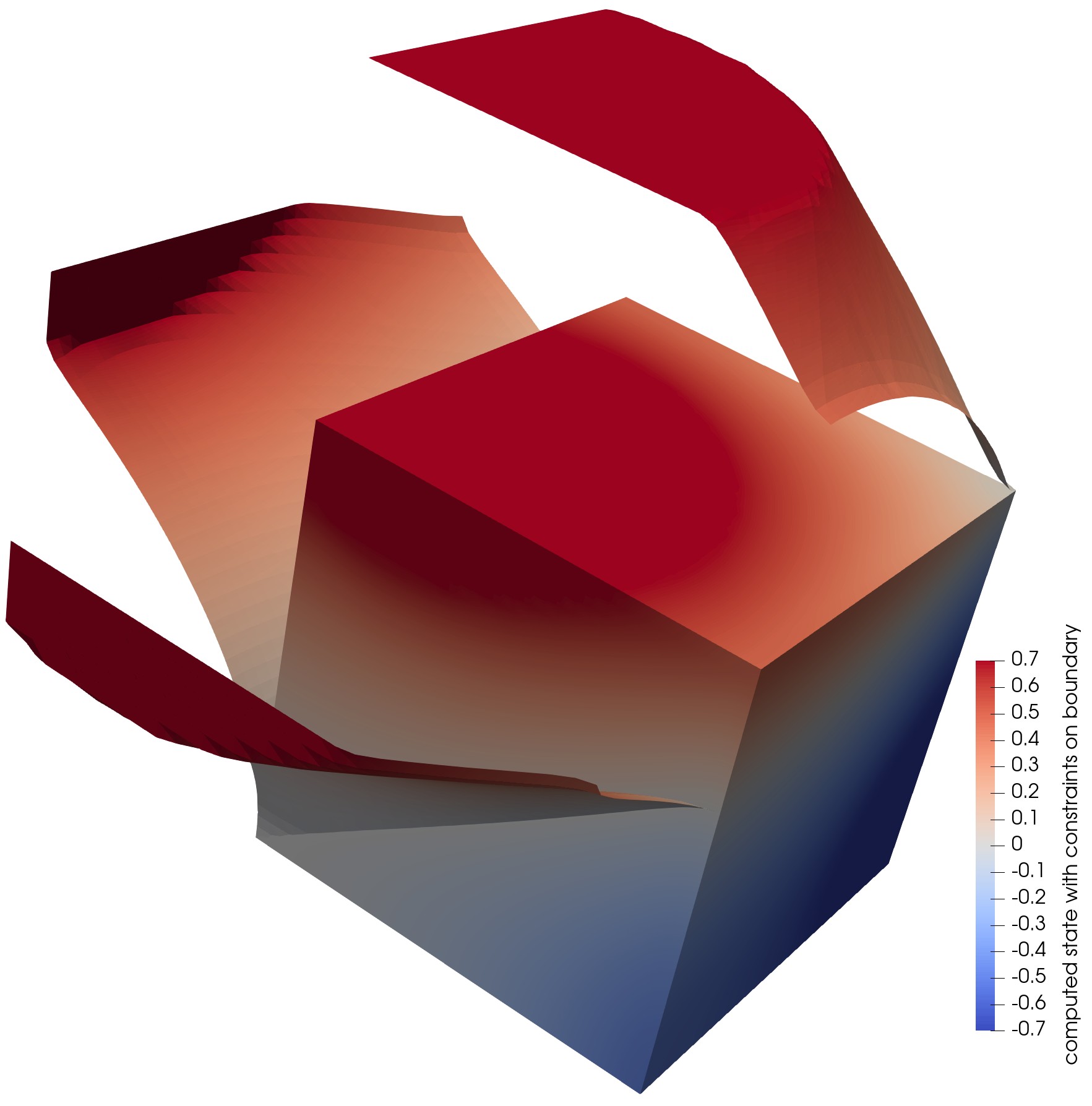
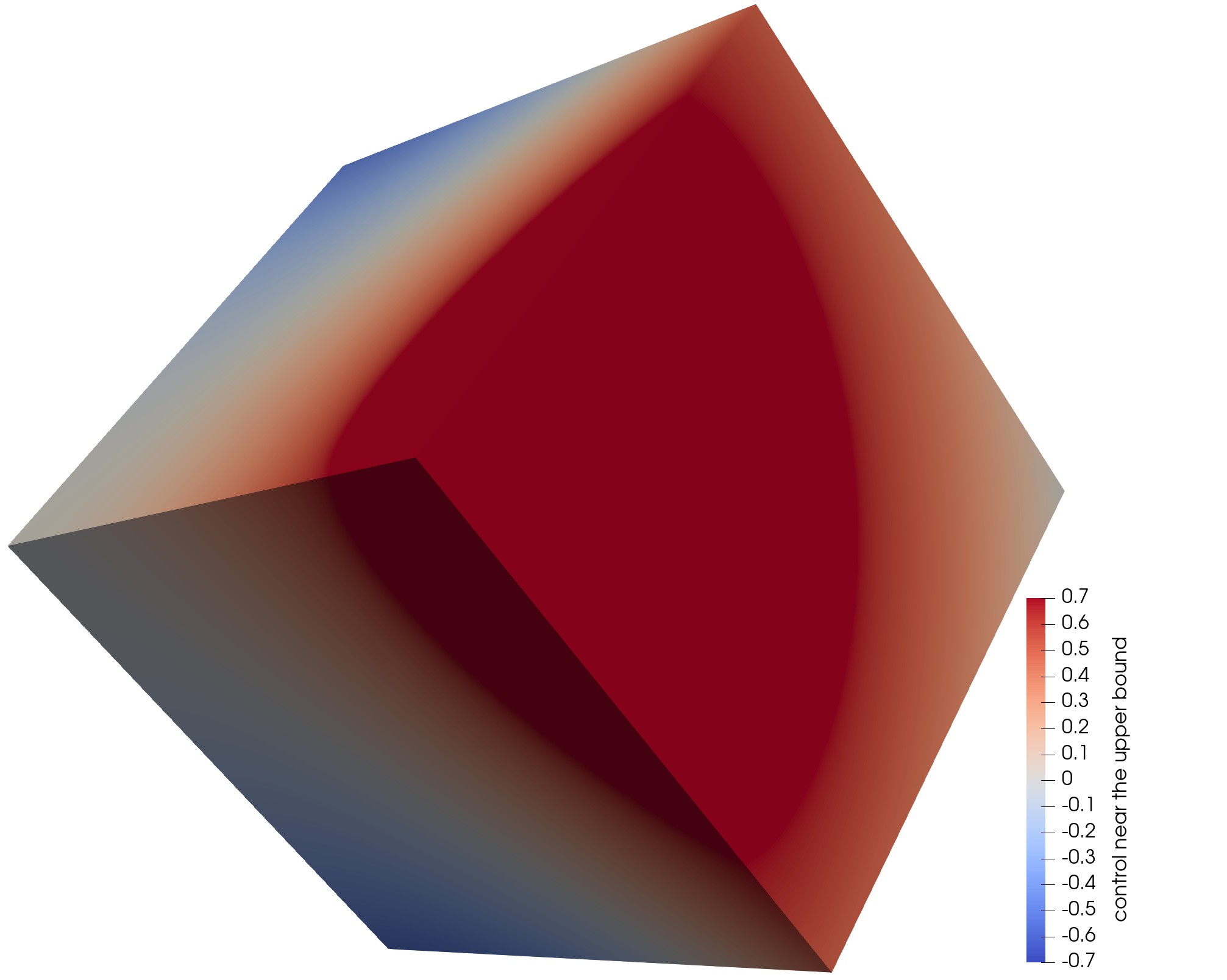
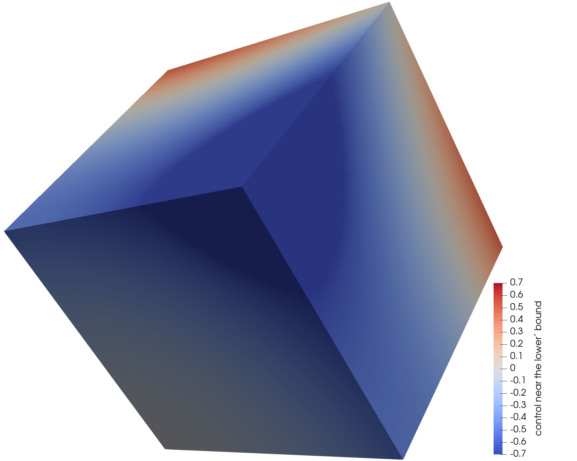
Figure 2: Visualization of the boundary control on three boundary parts (left), and near the upper (middle) and lower (right) bounds at level $6$.

7 Conclusions and outlook

We have presented a new approach to the numerical solution of optimal control problems for the Laplace equation where the Dirichlet boundary data serves as control. We have used energy regularization in $H^{1/2}(\Gamma)$ that is natural for Dirichlet data when considering the standard variational formulation of elliptic second order partial differential equations. We have reduced the optimality conditions to a variational equality for computing the state in the space of harmonic functions. For a practical realization, we have introduced a Lagrange multiplier leading to a mixed variational formulation in $H^{1}(\Omega)\times H^{1}_{0}(\Omega)$ that can easily be discretized by standard $C^{0}$ conforming finite elements. The analysis of the error in terms of the cost parameter $\varrho$ and the finite element mesh size $h$ implies that both parameters should appropriately be balanced in order to obtain asymptotically optimal convergence rates. It turns out that $\varrho=h^{2}$ in the case of 2D and 3D domains $\Omega$ with smooth boundaries $\Gamma$. If the boundary $\Gamma$ is only piecewise smooth, then the choice $\varrho=h^{2}$ is only suboptimal for smooth targets as it was shown theoretically in 2D, and numerically in 3D. Indeed, in 2D, it turns out that $\varrho=h^{2}/|\log(h)|$ is the optimal choice. Furthermore, we have proposed efficient solvers for the resulting system of finite element equations, and we have shown that it is easy to incorporate box constraints on the control and the state at once.

The precise analysis of smooth targets in 3D domains $\Omega$ with piecewise smooth boundaries, and the construction and implementation of asymptotically optimal solvers are interesting future research topics. It is clear that the Laplace operator plays the role of a model operator that can be replaced by other second-order elliptic partial differential operators. These and other optimal control problems fit into the abstract framework recently presented in [29]. We only mention here Neumann [10] and Robin boundary control, boundary and initial data control of parabolic initial-boundary value problems, partial distributed control, and targets given on a subset or even only on the boundary of the computational domain. In terms of inverse problems, the latter is also called partial or limited observation [33].

References

- [1] V. I. Agoshkov and V. I. Lebedev. Poincaré Steklov operators and methods of partition of the domain in variational problems. In G. I. Marchuk, editor, Compututational Processes and Systems 2, pages 173–227, Moscow, 1985. Nauka.
- [2] T. Apel, M. Mateos, J. Pfefferer, and A. Rösch. On the regularity of the solutions of Dirichlet optimal control problems in polygonal domains. SIAM J. Control Optim., 53:3620–3641, 2015.
- [3] N. Arada and J. P. Raymond. Dirichlet boundary control of semilinear parabolic equations. part 1: problems with no state constraints. Appl. Math. Optim., 45:125–143, 2002.
- [4] M. Arioli and D. Loghin. Discrete interpolation norms with applications. SIAM J. Numer. Anal., 47(4):2924–2951, 2009.
- [5] J. Behrndt, F. Gesztesy, and M. Mitrea. Sharp boundary trace theory and Schrödinger operators on bounded Lipschitz domains. Mem. Amer. Math. Soc., 307(1550):vi+208, 2025.
- [6] J. Behrndt and T. Micheler. Elliptic differential operators on Lipschitz domains and abstract boundary value problems. J. Funct. Anal., 267(10):3657–3709, 2014.
- [7] F. B. Belgacem, H. E. Fekih, and H. Metoui. Singular perturbations for the Dirichlet boundary control of elliptic problems. Math. Model. Numer. Anal., 37:833–850, 2003.
- [8] M. Berggren. Approximations of very weak solutions to boundary value problems. SIAM J. Numer. Anal., 42:860–877, 2004.
- [9] D. Braess and P. Peisker. On the numerical solution of the biharmonic equation and the role of squaring matrices for preconditioning. IMA J. Numer. Anal., 6:393–404, 1986.
- [10] S. Brenner and L.-Y. Sung. A new error analysis for finite element methods for elliptic Neumann boundary control problems with pointwise control constraints. Results Appl. Math., 25:100544, 2025.
- [11] F. Brezzi. On the existence, uniqueness and approximation of saddle-point problems arising from Lagrangian multipliers. RAIRO Anal. Numér., 8:129–151, 1974.
- [12] E. Casas. Boundary control of semilinear elliptic equations with pointwise state constraints. SIAM J. Control Optim., 31(4):993–1006, 1993.
- [13] E. Casas and J. P. Raymond. Error estimates for the numerical approximation of Dirichlet boundary control for semilinear elliptic equations. SIAM J. Control Optim., 45:1586–1611, 2006.
- [14] S. Chowdhury, T. Gudi, and A. K. Nandakumaran. Error bounds for a Dirichlet boundary control problem based on energy spaces. Math. Comput., 86(305):1103–1126, 2017.
- [15] P. G. Ciarlet and P. A. Raviart. A mixed finite element method for the biharmonic equation. In de Boor, editor, Mathematical aspects of finite elements in partial differential equations, pages 125–145, New York, 1974. Academic Press.
- [16] K. Deckelnick, A. Günther, and M. Hinze. Finite element approximation of Dirichlet boundary control for elliptic PDEs on two- and three-dimensional curved domains. SIAM J. Control Optim., 48:2798–2819, 2009.
- [17] A. V. Fursikov, M. D. Gunzburger, and L. S. Hou. Boundary value problems and optimal boundary control for the Navier-Stokes system: the two-dimensional case. SIAM J. Control Optim., 36:852–894, 1998.
- [18] P. Gangl, R. Löscher, and O. Steinbach. Regularization and finite element error estimates for elliptic distributed optimal control problems with energy regularization and state or control constraints. Comput. Math. Appl., 180:242–260, 2025.
- [19] R. Glowinski and O. Pironneau. Numerical methods for the first biharmonic equation and for the two-dimensional Stokes problem. SIAM Rev,, 21:167–212, 1979.
- [20] M. D. Gunzburger, L. Hou, and T. P. Svobodny. Boundary velocity control of incompressible flow with an application to viscous drag reduction. SIAM J. Control Optim., 30:167–181, 1992.
- [21] M. Hintermüller, K. Ito, and K. Kunisch. The primal-dual active set strategy as a semismooth Newton method. SIAM J. Optim., 13:865–888, 2003.
- [22] M. Hinze and K. Kunisch. Second order methods for boundary control of the instationary Navier–Stokes system. Z. Angew. Math. Mech., 84:171–187, 2004.
- [23] M. Hinze, R. Pinnau, M. Ulbrich, and S. Ulbrich. Optimization with PDE Constraints, volume 23 of Mathematical Modelling: Theory and Applications. Springer, Heidelberg, 2009.
- [24] L. John and O. Steinbach. Schur complement preconditioners for the biharmonic Dirichlet boundary value problem. Berichte aus dem Institut für Numerische Mathematik, 2013/4, TU Graz, 2013.
- [25] M. Jung, U. Langer, A. Meyer, W. Queck, and M. Schneider. Multigrid preconditioners and their applications. In G. Telschow, editor, Third Multigrid Seminar, Biesenthal 1988, pages 11–52, Karl–Weierstrass–Institut, Berlin, Report R–MATH–03/89, 1989.
- [26] K. Kunisch and B. Vexler. Constrained Dirichlet boundary control in for a class of evolution equations. SIAM J. Control Optim., 46:1726–1753, 2007.
- [27] U. Langer. Zur numerischen Lösung des ersten biharmonischen Randwertproblems. Numer. Math., 50(3):291–310, 1986.
- [28] U. Langer, R. Löscher, O. Steinbach, and H. Yang. Mass-lumping discretization and solvers for distributed elliptic optimal control problems. Numer. Linear Algebra Appl., 31(5):e2564, 2024.
- [29] U. Langer, R. Löscher, O. Steinbach, and H. Yang. State-based nested iteration solution of optimal control problems with PDE constraints, 2025. arXiv:2505.19062.
- [30] I. Lasiecka and K. Malanowski. On discrete-time Ritz-Galerkin approximation of control constrained optimal control problems for parabolic systems. Control Cybern., 7:21–36, 1978.
- [31] D. Liang, W. Gong, and X. Xie. A new error analysis for parabolic Dirichlet boundary control problems. ESAIM: Math. Modelling Numer. Anal., 59:749–787, 2025.
- [32] J. L. Lions. Optimal Control of Systems Governed by Partial Differential Equations. Springer, Berlin, 1971.
- [33] K.-A. Mardal, B. Nielsen, and M. Nordaas. Robust preconditioners for pde-constrained optimization with limited observations. BIT Numer. Math., 57:405–431, 2017.
- [34] S. May, R. Rannacher, and B. Vexler. Error analysis for a finite element approximation of elliptic Dirichlet boundary control problems. SIAM J. Control Optim., 51:2585–2611, 2013.
- [35] W. McLean. Strongly Elliptic Systems and Boundary Integral Equations. Cambridge University Press, 2000.
- [36] W. McLean and O. Steinbach. Boundary element preconditioners for a hypersingular integral equation on an interval. Adv. Comput. Math., 11:271–286, 1999.
- [37] G. Of, T. X. Phan, and O. Steinbach. An energy space finite element approach for elliptic Dirichlet boundary control problems. Numer. Math., 129:723–748, 2015.
- [38] P. Peisker. On the numerical solution of the first biharmonic equation. RAIRO Modél. Math. Anal. Numér., 22(4):655–676, 1988.
- [39] A. Quarteroni and A. Valli. Numerical Approximation of Partial Differential Equations, volume 23 of Springer Series in Computational Mathematics. Springer, Berlin, Heidelberg, 1994.
- [40] A. Quarteroni and A. Valli. Domain Decomposition Methods for Partial Differential Equations. Oxford Science Publications, 1999.
- [41] J. Ruge and K. Stüben. Algebraic multigrid. In S. McCormick, editor, Multigrid Methods, Frontiers in Applied Mathematics, chapter 4, pages 73–130. SIAM, Philadelphia, 1987.
- [42] O. Steinbach. On the stability of the projection in fractional Sobolev spaces. Numer. Math., 88:367–379, 2001.
- [43] O. Steinbach. On a generalized projection and some related stability estimates in Sobolev spaces. Numer. Math., 90:775–786, 2002.
- [44] O. Steinbach. Numerical approximation methods for elliptic boundary value problems. Finite and boundary elements. Springer, New York, 2008.
- [45] F. Tröltzsch. Optimal Control of Partial Differential Equations: Theory, Methods and Applications, volume 12 of Graduate Studies in Mathematics. AMS, Providence, Rhode Island, 2010.
- [46] S. Zhang and J. Xu. Optimal solvers for fourth-order PDEs discretized on unstructured grids. SIAM J. Numer. Anal., 52:282–307, 2014.