Higher-Order Fermion Interactions in BCS Theory

D. Rodriguez-Gomez^a,b and J. G. Russo ^c,d

^a Department of Physics, Universidad de Oviedo

C/ Federico García Lorca 18, 33007 Oviedo, Spain

^b Instituto Universitario de Ciencias y Tecnologías Espaciales de Asturias (ICTEA)

C/ de la Independencia 13, 33004 Oviedo, Spain.

^c Institució Catalana de Recerca i Estudis Avançats (ICREA)

Pg. Lluis Companys, 23, 08010 Barcelona, Spain

^d Departament de Física Cuántica i Astrofísica and Institut de Ciències del Cosmos

Universitat de Barcelona, Martí Franquès, 1, 08028 Barcelona, Spain

ABSTRACT

We investigate the impact of higher-order fermionic deformations in multiflavor Bardeen-Cooper-Schrieffer (BCS) theory. Focusing specifically on the 6- and 8-fermion interactions, we show that these terms can have significant consequences on the dynamics of the system. In certain regions of parameter space, the theory continues to exhibit second-order phase transitions with mean-field critical exponents and the same critical temperature; however, the temperature dependence of the superconducting gap can deviate markedly from conventional BCS behavior. In other regions, the theory exhibits first-order phase transitions or second-order phase transitions with non-mean field exponents. We conclude by discussing potential phenomenological applications of these theories.

1 Introduction

The Bardeen-Cooper-Schrieffer (BCS) theory of superconductivity remains as a major achievement of the 20th century Physics [1]. Through phonon interactions, electrons feel an effective quartic interaction which forces them to condense into Cooper pairs driving superconductivity. Yet, from the perspective of effective field theory, it remains surprising that a quartic fermionic interaction can produce such a pronounced effect. Naive power-counting suggests that the quartic coupling is an irrelevant interaction in spacetime dimensions greater than two. However, as argued in [2], the presence of the Fermi surface significantly modifies the naive scaling, making the quartic coupling marginally relevant in specific kinematic regimes. This observation naturally raises the question of how this effect might propagate in the presence of higher-order couplings. It is indeed reasonable to expect that the RG flow will mix the running of the various couplings, so that the infrared relevance of the quartic interaction will, in general, extend to and influence the behavior of the higher-order terms.

In this paper we set out to study this question in detail. For concreteness, we restrict our analysis to a class of models with $\psi^{6}$ and $\psi^{8}$ interactions. As we will see, depending on the coefficients of the higher-order fermionic couplings, the transition can be second order or first order. When the $\psi^{6}$ interaction is absent, the transition is second order below a certain critical value of the $\psi^{8}$ coupling. In this case, the critical exponents still have mean-field values, but the gap curve is deformed as compared with the BCS prediction. In presence of the $\psi^{6}$ interaction, second-order transitions are still possible in a range of parameters, but with non-mean field exponents. In another range of parameters, higher-order couplings drive the system into a regime where the phase transition becomes first-order. We will discuss potential phenomenological applications of the various scenarios in section 5.

2 The model

Our starting point is the familiar non-relativistic Lagrangian describing the BCS model, extended to $N$ fermionic flavors as in [3],

$$\mathcal{L}=\sum_{a=1}^{N}\sum_{\sigma=\uparrow,\downarrow}\bar{\psi}_{a,\,\sigma}\Big{(}\partial_{\tau}-\frac{\vec{\partial}^{2}}{2m}-\mu\Big{)}\psi_{a,\,\sigma}-\frac{g}{N}\,(\sum_{a=1}^{N}\bar{\psi}_{a,\uparrow}\bar{\psi}_{a,\downarrow})\,(\sum_{b=1}^{N}\psi_{b,\downarrow}\psi_{b,\uparrow})\ .$$ (2.1)

This model assumes a $SO(N)\times U(1)_{e}$ continuous global symmetry under which $\vec{\psi}_{\uparrow}$ transforms as $\mathbf{N}_{1}$ while $\vec{\psi}_{\downarrow}$ as a $\mathbf{\overline{N}}_{1}$.

Introducing a Hubbard-Stratonovich field $\Delta$ transforming in the $\mathbf{1}_{-2}$, one writes the equivalent Lagrangian

$$\mathcal{L}^{\prime}=\sum_{a=1}^{N}\sum_{\sigma=\uparrow,\downarrow}\bar{\psi}_{a,\,\sigma}\Big{(}\partial_{\tau}-\frac{\vec{\partial}^{2}}{2m}-\mu\Big{)}\psi_{a,\,\sigma}-\Delta\,(\sum_{a=1}^{N}\bar{\psi}_{a,\uparrow}\bar{\psi}_{a,\downarrow})-\bar{\Delta}\,(\sum_{b=1}^{N}\psi_{b,\downarrow}\psi_{b,\uparrow})+\frac{N}{g}\Delta\bar{\Delta}\,.$$ (2.2)

It is worth noting that, more generically, we could have considered an interaction $\Delta_{ab}\,\bar{\psi}_{a,\uparrow}\bar{\psi}_{b,\downarrow}+{\rm h.c.}$ exhibiting a $U(N)\times U(N)$ global symmetry; of which our model is a restriction. This generic class also includes the models describing the so-called Type 1.5 superconductors [4].

The equation of motion for $\Delta$ and $\bar{\Delta}$ sets

$$\bar{\Delta}=\frac{g}{N}\,(\sum_{a=1}^{N}\bar{\psi}_{a,\uparrow}\bar{\psi}_{a,\downarrow})\,,\qquad\Delta=\frac{g}{N}\,(\sum_{b=1}^{N}\psi_{b,\downarrow}\psi_{b,\uparrow})\,.$$ (2.3)

Substituting back into $\mathcal{L}^{\prime}$ we recover the original Lagrangian $\mathcal{L}$.

As described in the introduction, we are interested in exploring the effect of a priori irrelevant couplings. Thus, we now add $\psi^{6}$ and $\psi^{8}$ deformations by introducing two new auxiliary fields $\Sigma$ and $\Phi$ as follows

$$\mathcal{L}^{\prime}= \sum_{a=1}^{2}\sum_{\sigma=\uparrow,\downarrow}\bar{\psi}_{a,\,\sigma}\Big{(}\partial_{\tau}-\frac{\vec{\partial}^{2}}{2m}-\mu\Big{)}\psi_{a,\,\sigma}-\Delta\,(\sum_{a=1}^{N}\bar{\psi}_{a,\uparrow}\bar{\psi}_{a,\downarrow})-\bar{\Delta}\,(\sum_{b=1}^{N}\psi_{b,\downarrow}\psi_{b,\uparrow})+\frac{N}{g}\Delta\bar{\Delta}$$

$$-(\kappa\,\Sigma^{2}+\lambda\,\Phi^{3})\,(\sum_{a=1}^{N}\psi_{a,\downarrow}\psi_{a,\uparrow}+\bar{\psi}_{a,\uparrow}\bar{\psi}_{a,\downarrow})+\frac{2}{3}\,\kappa\,N\,\Sigma^{3}+\frac{3}{4}\,\lambda\,N\,\Phi^{4}\,.$$ (2.4)

The equations of motion for $\Sigma$ and $\Phi$ set

$$\Sigma=\frac{1}{N^{2}}\,\left(\sum_{a=1}^{N}\left(\psi_{a,\downarrow}\psi_{a,\uparrow}+\bar{\psi}_{a,\uparrow}\bar{\psi}_{a,\downarrow}\right)\right)^{2}\,\,,\qquad\Phi=\frac{1}{N^{3}}\,\left(\sum_{a=1}^{N}\left(\psi_{a,\downarrow}\psi_{a,\uparrow}+\bar{\psi}_{a,\uparrow}\bar{\psi}_{a,\downarrow}\right)\right)^{3}\,.$$ (2.5)

Integrating out the auxiliary field $\Delta$ as well, we obtain

$$\mathcal{L}= \sum_{a=1}^{N}\sum_{\sigma=\uparrow,\downarrow}\bar{\psi}_{a,\,\sigma}\Big{(}\partial_{\tau}-\frac{\vec{\partial}^{2}}{2m}-\mu\Big{)}\psi_{a,\,\sigma}-\frac{g}{N}\,(\sum_{a=1}^{N}\bar{\psi}_{a,\uparrow}\bar{\psi}_{a,\downarrow})\,(\sum_{b=1}^{N}\psi_{b,\downarrow}\psi_{b,\uparrow})$$

$$-\frac{\kappa}{3N^{2}}\,(\sum_{a=1}^{N}\psi_{a,\downarrow}\psi_{a,\uparrow}+\bar{\psi}_{a,\uparrow}\bar{\psi}_{a,\downarrow})^{3}-\frac{\lambda}{4N^{3}}\,(\sum_{a=1}^{N}\psi_{a,\downarrow}\psi_{a,\uparrow}+\bar{\psi}_{a,\uparrow}\bar{\psi}_{a,\downarrow})^{4}\,.$$ (2.6)

Stability requires $\lambda\geq 0$. When $\lambda=0$ we must require $\kappa>0$, while for $\lambda>0$ the coupling $\kappa$ can take any arbitrary real value.

The Lagrangian section 2 may be viewed as the microscopic model. It is important to stress that this is only one out of many possible models: not only one could consider higher $\psi^{n}$ terms, but also, for generic $N$, typically there exist various possible contractions of the flavor indices contributing to a given $\psi^{n}$ interaction. In particular, we have chosen to preserve only the continuous $SO(N)$ symmetry. Note that, due to the Grassmann nature of the fermionic field, for any given $N$ and sufficiently large $n$, the interaction terms vanish. For instance, for $N=1$ all $\psi^{n}$ interactions with $n>4$ vanish. For $N=2$ all $\psi^{n}$ terms with $n>8$ vanish and the $\psi^{8}$ interaction is unique, given by

$$-\frac{6\lambda}{N^{2}}(\bar{\psi}_{1,\uparrow}\bar{\psi}_{1,\downarrow})\,(\psi_{1,\downarrow}\psi_{1,\uparrow})(\bar{\psi}_{2,\uparrow}\bar{\psi}_{2,\downarrow})\,(\psi_{2,\downarrow}\psi_{2,\uparrow})\ .$$

Additional (discrete) symmetries might restrict the possible interactions. In particular, a $\mathbb{Z}_{4}$ symmetry inside the $U(1)_{e}$ acting as $\psi_{a,\sigma}\rightarrow i\,\psi_{a,\sigma}$ would force the $\psi^{6}$ term to vanish. In this case, for $N=2$, the Lagrangian (2) with $\kappa=0$ would represent the most general Lagrangian consistent with the symmetries.

2.1 Integrating out the fermions

Writing the model as in section 2, the fermions appear quadratically and hence can be integrated out. Let us introduce

$$\Psi_{a}=\left(\begin{array}[]{c}\psi_{a,\uparrow}\\ \bar{\psi}_{a,\downarrow}\end{array}\right)\,,\qquad\Psi^{\dagger}_{a}=(\bar{\psi}_{a,\uparrow},\,\psi_{a,\downarrow})\,,$$ (2.7)

and

$$\mathcal{A}=\left(\begin{array}[]{cc}-\partial_{\tau}+\frac{\vec{\partial}^{2}}{2m}+\mu&\Delta+\kappa\Sigma^{2}+\lambda\Phi^{3}\\ \bar{\Delta}+\kappa\Sigma^{2}+\lambda\Phi^{3}&-\partial_{\tau}-\frac{\vec{\partial}^{2}}{2m}-\mu\end{array}\right)\,.$$ (2.8)

Then section 2 becomes

$$\mathcal{L}=\sum_{a=1}^{N}\Psi_{a}^{\dagger}\,\mathcal{A}\,\Psi_{a}+\frac{N}{g}\Delta\bar{\Delta}+\frac{2\kappa N}{3}\Sigma^{3}+\frac{3\lambda N}{4}\Phi^{4}\,.$$ (2.9)

Integrating out the $N$ fermions, the one-loop effective Lagrangian becomes

$$\mathcal{L}_{\rm 1-loop}=N\,\left(-\mathcal{D}+\frac{1}{g}\Delta\bar{\Delta}+\frac{2\kappa}{3}\Sigma^{3}+\frac{3\lambda}{4}\Phi^{4}\right)\ .$$ (2.10)

For the theory at finite temperature, $\mathcal{D}\equiv{\rm Tr}\log\mathcal{A}$ is given by

$$\mathcal{D}=T\,\sum_{n}\int\frac{d^{d}\vec{k}}{(2\pi)^{d}}\,\log\big{[}\big{(}(2n+1)\pi T\big{)}^{2}+\xi^{2}+|\Delta+\kappa\Sigma^{2}+\lambda\Phi^{3}|^{2}\big{]}\,,$$ (2.11)

where

$$\xi=\frac{\vec{k}^{2}}{2m}-\mu\,.$$ (2.12)

Note that $\mathcal{D}=\mathcal{D}(X)$, with $X=|\Delta+\kappa\Sigma^{2}+\lambda\Phi^{3}|$. The equations of motion for $\bar{\Delta}$, $\Delta$ are given by

$$-(\Delta+\kappa\Sigma^{2}+\lambda\Phi^{3})\mathcal{D}^{\prime}(X)+\frac{\Delta}{g}=0\,,\qquad\,-(\bar{\Delta}+\kappa\Sigma^{2}+\lambda\Phi^{3})\mathcal{D}^{\prime}(X)+\frac{\bar{\Delta}}{g}=0\ ,$$ (2.13)

where we have introduced the notation $\mathcal{D}^{\prime}\equiv\partial\mathcal{D}/\partial X$. As usual, one can set $\bar{\Delta}=\Delta$. Then the equations for $\Sigma$ and $\Phi$ become

$$-\Sigma(\Delta+\kappa\Sigma^{2}+\lambda\Phi^{3})\mathcal{D}^{\prime}(X)+\Sigma^{2}=0\,,\qquad-\Phi^{2}(\Delta+\kappa\Sigma^{2}+\lambda\Phi^{3})\mathcal{D}^{\prime}(X)+\Phi^{3}=0\,,$$ (2.14)

Combining these equations, we find

$$\Sigma=\frac{1}{g}\,\Delta\,,\qquad\Phi=\frac{1}{g}\,\Delta\,.$$ (2.15)

We are finally then left with a single equation, which reads

$$\left(-(1+b\Delta+c\Delta^{2})\mathcal{D}^{\prime}+\frac{1}{g}\right)\Delta=0\,.$$ (2.16)

where

$$b\equiv\frac{\kappa}{g^{2}}\ ,\qquad c\equiv\frac{\lambda}{g^{3}}\ ,$$ (2.17)

and $\mathcal{D}^{\prime}$ is evaluated at $\Sigma$ and $\Phi$ given by (2.15).

Equation 2.16 has the trivial solution $\Delta=0$, which represents the uncondensed phase. In addition, there can be non-trivial solutions representing condensed phases, where the gap is determined by the equation

$$(1+b\Delta+c\Delta^{2})\,\mathcal{D}^{\prime}=\frac{1}{g}\ .$$ (2.18)

In order to further proceed, we now need to compute $\mathcal{D}^{\prime}(X)$. Explicitly, it reads

$$\mathcal{D}^{\prime}=T\,\sum_{n}\,\int\frac{d^{d}\vec{k}}{(2\pi)^{d}}\,\frac{1}{\big{(}(2n+1)\pi T\big{)}^{2}+\xi^{2}+\Delta^{2}\,\eta^{2}}\,,$$ (2.19)

where

$$\eta\equiv 1+b\Delta+c\Delta^{2}\ .$$ (2.20)

Performing the sum, one finds

$$\mathcal{D}^{\prime}=\frac{1}{2}\,\int\frac{d^{d}\vec{k}}{(2\pi)^{d}}\,\frac{\tanh\frac{\sqrt{\xi^{2}+\Delta^{2}\,\eta^{2}}}{2T}}{\sqrt{\xi^{2}+\Delta^{2}\,\eta^{2}}}\,.$$ (2.21)

Integrating, we find

$$\mathcal{D}=\int\frac{d^{d}\vec{k}}{(2\pi)^{d}}\Big{[}\sqrt{\xi^{2}+\Delta^{2}\,\eta^{2}}+2T\,\log\frac{1}{2}\Big{(}1+e^{-\frac{\sqrt{\xi^{2}+\Delta^{2}\,\eta^{2}}}{T}}\Big{)}\Big{]}\,.$$ (2.22)

This formula will be used in the calculation of the free energy.

In standard BCS theory, one assumes that the relevant dynamics takes place near the Fermi surface. Under this assumption, one can approximate

$$\int\frac{d^{d}\vec{k}}{(2\pi)^{d}}\sim\nu\,\int_{-\omega_{*}}^{\omega_{\star}}d\xi\,,$$ (2.23)

where $\omega_{\star}$ is the Debye energy (playing the role of a physical cutoff) and $\nu$ is the density of states at the Fermi level, defined by a $\xi(k)=\frac{k^{2}}{2m}-\mu=0$. The final form of the gap equation is therefore:

$$\frac{1}{g\,\nu\,(1+b\Delta+c\,\Delta^{2})}=\int_{0}^{\omega_{\star}}d\xi\,\frac{\tanh\frac{\sqrt{\xi^{2}+\Delta^{2}\,\eta^{2}}}{2T}}{\sqrt{\xi^{2}+\Delta^{2}\,\eta^{2}}}\,.$$ (2.24)

The new terms with coefficients $b$ and $c$ represent corrections to standard BCS theory and cannot be absorbed into a redefinition of $\Delta$.

2.2 Free energy

The free energy is obtained by computing the action evaluated on the solution. This yields (we set $\Delta=\bar{\Delta}$)

$$\frac{F}{N}=\frac{1}{g}\Delta^{2}+\frac{2}{3\kappa}\Sigma^{\frac{3}{2}}+\frac{3}{4\lambda}\Phi^{\frac{4}{3}}-\int\frac{d^{d}\vec{k}}{(2\pi)^{d}}\Big{[}\sqrt{\xi^{2}+\Delta^{2}\,\eta^{2}}+2T\,\log\frac{1}{2}\Big{(}1+e^{-\frac{\sqrt{\xi^{2}+\Delta^{2}\,\eta^{2}}}{T}}\Big{)}\Big{]}\,.$$ (2.25)

Choosing the uncondensed state –with free energy $F_{0}$– as the reference, the free-energy difference $f\equiv\frac{1}{N}(F-F_{0})$ is

$$f=\frac{1}{g}\Delta^{2}+\frac{4\,b}{3\,g}\,\Delta^{3}+\frac{3\,c}{2\,g}\,\Delta^{4}-\int\frac{d^{d}\vec{k}}{(2\pi)^{d}}\Big{[}\big{(}\sqrt{\xi^{2}+\Delta^{2}\,\eta^{2}}-\xi\big{)}+2T\,\log\Big{(}\frac{1+e^{-\frac{\sqrt{\xi^{2}+\Delta^{2}\,\eta^{2}}}{T}}}{1+e^{-\frac{\xi}{T}}}\Big{)}\Big{]}\,,$$ (2.26)

Assuming the same approximation as in eq. 2.23 for the momentum integral we find

$$f=\frac{1}{g}\Delta^{2}+\frac{4\,b}{3\,g}\,\Delta^{3}+\frac{3\,c}{2\,g}\,\Delta^{4}-2\nu\int_{0}^{\omega_{\star}}d\xi\Big{[}\big{(}\sqrt{\xi^{2}+\Delta^{2}\,\eta^{2}}-\xi\big{)}+2T\,\log\Big{(}\frac{1+e^{-\frac{\sqrt{\xi^{2}+\Delta^{2}\,\eta^{2}}}{T}}}{1+e^{-\frac{\xi}{T}}}\Big{)}\Big{]}\,.$$ (2.27)

3 Analysis of the condensed phase

In this section, an analytical study of the possible condensed phases is carried out by examining the gap equation eq. 2.24.

3.1 The $T=0$ limit

We first consider the small temperature region. As $T\rightarrow 0$, the $\tanh$ in eq. 2.24 goes to one, and the integral can be computed explicitly. One finds the following equation for $\Delta_{0}\equiv\Delta(T=0)$:

$$\eta_{0}\,\Delta_{0}=\frac{\omega_{\star}}{\sinh(1/(g\,\nu\,\eta_{0}))}\ ,\qquad\eta_{0}\equiv 1+b\Delta_{0}+c\Delta_{0}^{2}\ .$$ (3.1)

This is a transcendental equation for $\Delta$ that can be solved numerically. The BCS case $b=c=0$ gives an estimate, which also applies to cases where $b$ and $c$ are small,

$$\Delta_{0}\approx\frac{\omega_{\star}}{\sinh(1/g\nu)}\ ,\qquad{\rm for}\ \ b\Delta_{0}+c\Delta_{0}^{2}\ll 1\ .$$ (3.2)

3.2 Expansion near the critical temperature

Assuming that $\Delta(T)$ vanishes at a critical temperature $T_{c}$, we have

$$\frac{1}{g\nu}=\int_{0}^{\frac{\omega_{\star}}{T_{c}}}\frac{\tanh\frac{x}{2}}{x}\approx\log\frac{k\omega_{\star}}{T_{c}}\,,\quad k\approx 1.134\qquad\leadsto\qquad T_{c}\approx k\,\omega_{\star}e^{-\frac{1}{g\nu}}\ .$$ (3.3)

Note that the critical temperature $T_{c}$ at which the gap vanishes, $\Delta=0$, is the same as in BCS theory since in this case the corrections with $b$ and $c$ coefficients vanish. However, because $\Delta$ can in principle be multivalued, the temperature $T_{c}$ may not be the critical temperature of the onset of the phase transition. In section 4 we will examine instances in which the system undergoes a first-order phase transition at a higher critical temperature $T_{c}^{\star}$.

The region close to $T_{c}$ is amenable to analytical treatment. Let us expand the gap equation around $T_{c}$. Defining $\delta T=T_{c}-T$ and neglecting $O(\Delta^{3})$ terms, we get

$$\alpha_{1}\,\delta T+\frac{b}{g\nu}\Delta-\left(\beta_{0}+\frac{b^{2}-c}{g\nu}\right)\,\Delta^{2}=0\,.$$ (3.4)

where

$$\alpha_{1}=\frac{1}{2T_{c}}\,\int_{0}^{\frac{\omega_{\star}}{T_{c}}}dx\,\frac{1}{\cosh^{2}\frac{x}{2}}\,,\qquad\beta_{0}=\frac{1}{4T_{c}^{2}}\,\int_{0}^{\frac{\omega_{\star}}{T_{c}}}dx\ \frac{1}{x^{3}\,\cosh^{2}\frac{x}{2}}\,\left(\sinh(x)-x\right)\,.$$ (3.5)

The behavior of the solution crucially depends on $b$:

• $b>0$: In this case the quadratic term in $\Delta$ may be neglected near $T_{c}$ and we have

  $$\Delta\approx\frac{g\nu}{b}\,\alpha_{1}\,(T-T_{c})\,.$$ (3.6)

  Since $\alpha_{1}>0$, the gap is non-vanishing for $T>T_{c}$. As we will see, this apparent “retrograde” condensation signals a non-single valued $\Delta(T)$ where the lower branch does not contribute to the thermodynamics because it represents a solution with more free energy than another branch occurring for larger $\Delta$. In this regime the system undergoes a first-order phase transition at a (different) critical temperature $T_{c}^{\star}$.

• $b<0$: This case requires $c>0$ for stability (unlike the case $b>0$ where one can consider a model with $c=0$). Near the critical temperature, in the linearized approximation the gap is given by (3.6), but now $\Delta\neq 0$ for $T<T_{c}$. This branch may or may not be physically relevant, as this depends on the existence of other possible branches occurring at larger values of $\Delta$. In turn, this depends on the values of the parameters, in particular, the values of the couplings $b$ and $c$. Examples will be given in section 4.

• $b=0$: in this case it follows that

  $$\Delta^{2}=\frac{\alpha_{1}}{\beta_{0}-\frac{c}{g\nu}}\,\delta T\,.$$ (3.7)

  Thus we have a second order transition provided $\beta_{0}-\frac{c}{g\nu}>0$, and first order otherwise. The critical $c$ happens at $c_{0}=g\nu\,\beta_{0}$. Explicitly

  $$c_{0}=\frac{1}{4T_{c}^{2}}\,\frac{\int_{0}^{\frac{\omega_{\star}}{T_{c}}}\frac{1}{x^{3}\,\cosh^{2}\frac{x}{2}}\,(\sinh x-x)}{\int_{0}^{\frac{\omega_{\star}}{T_{c}}}\frac{\tanh\frac{x}{2}}{x}}\approx n_{0}\,\frac{g\nu}{4T_{c}^{2}},\ \ n_{0}\approx 0.426\,,$$ (3.8)

  where the integral in the numerator has been estimated assuming that $\omega_{\star}\gg T_{c}$. In order to study the behavior right at the critical coupling $c=c_{0}$, we need to keep the next order in the gap $\Delta(T)$, leading to

  $$\Delta^{4}=\gamma\,(T_{c}-T)+O(\delta T^{2})\ ,\qquad\gamma>0\ .$$ (3.9)

  Thus, at this critical coupling $c_{0}$, the critical exponent is $1/4$.

  To provide further support for this picture, we can calculate the free energy near $T_{c}$. We find

  $$f\sim\frac{1}{2}\,\frac{\alpha_{1}^{2}\,\nu}{(\beta_{0}-\frac{c}{g\nu})}\,\delta T^{2}+\cdots\,.$$ (3.10)

  Thus we see that $f$ precisely changes sign at $c=c_{0}$ and goes from a negative to a positive concavity at $T_{c}$, consistent with the change from a second to a first order phase transition (cf. red, black and blue vs. green curves in fig. 2 below).

Just as in conventional BCS (type I) superconductors, the Meissner effect dictates the temperature dependence of the critical magnetic field. One has

$$\frac{1}{2}H_{c}(T)^{2}=Nf(T)\ .$$ (3.11)

For $b=0$ and $c<c_{0}$, near the critical temperature, using (3.10), one obtains the usual behavior

$$H_{c}(T)\approx H_{c}(0)\left(1-\left(\frac{T}{T_{c}}\right)^{2}\right)\ .$$ (3.12)

Away from the critical temperature, in regions where $\Delta$ is not small, there will be deviations from BCS, but the phase diagram will be qualitatively the same.

4 Numerical analysis of the condensed phase

In this section we numerically solve the gap equation and compute the free energy of the system for different values of the parameters.

4.1 $\psi^{8}$ interaction ($b=0$)

We start with the case of the $\psi^{8}$ interaction alone, corresponding to $b=0$ and $c>0$. According to the analysis of the previous section, the theory with $c<c_{0}$ should exhibit a second order phase transition with critical exponent $1/2$ ($1/4$ for the fine-tuned case $c=c_{0}$) and a first order phase transition in the regime $c>c_{0}$. This is supported by fig. 1, where we show the numerical solution to the gap equation for $\Delta$ as a function of the temperature for different values of $c$. For $c<c_{0}$ (red and black curves) the curve has a similar behavior to the standard BCS case. In turn, for $c>c_{0}$ (green curve), $\Delta$ develops a lump (in the case at hand, reaching up to $T_{0}\sim 4.5$) and becomes non-single valued in the range $T\in(T_{c},\,T_{0})$, indicating the presence of a first order phase transition in this regime.

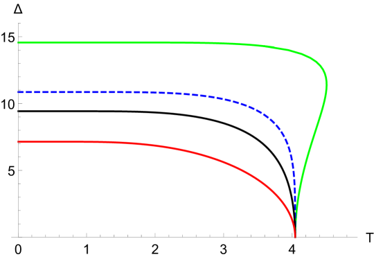
Figure 1: $\Delta$ vs. $T$ for $b=0$ (standard BCS) and $c=0$ (red), $c=0.8\,c_{0}$ (black), $c=c_{0}$ (dashed, blue), $c=1.2\,c_{0}$ (green). Here $g\nu=0.3$, $\omega_{\star}=100$.

This scenario can be explicitly tested by computing the free energy in each case as shown in fig. 2. For $c>c_{0}$ the free energy exhibits the characteristic swallowtail of a first-order phase transition showing that at some $T_{c}^{\star}$ ($\sim 4.3$ in the example shown) there is a first order phase transition.

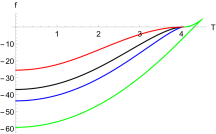
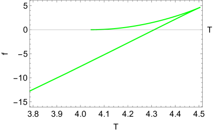
(a)	(b)

Figure 2: a) Free energy vs. $T$ (same conventions as in figure 1). b) Enlarged view of the free energy in the case $c=1.2\,c_{0}$. The lower branch in Fig. 1 corresponds to the branch with positive free energy. The upper branch in figure 1 has negative free energy until $T^{\star}_{c}\approx 4.3$, where a first-order phase transition takes place. For $T>T^{\star}_{c}$, $\Delta=0$.

Although the critical exponents in the region $c<c_{0}$ remain the same as in mean-field theory and match those of the BCS theory, the temperature dependence of the gap exhibits a qualitatively distinct profile compared to the BCS case (cf. the black curve with the BCS curve in red in fig. 1).

4.2 $\psi^{6}$ interaction ($c=0$)

We now consider the case of the $\psi^{6}$ interaction alone. Recall that this case requires $b>0$. Solving the gap equation for this case one finds the picture illustrated in fig. 3. The $\Delta(T)$ curve is not single-valued in the interval $T\in(T_{c},\,T_{0})$ with $T_{c}\approx 4.04$ and $T_{0}\approx 6.3$, again indicating the presence of a first order phase transition. This can be verified computing the free energy, which is shown in fig. 3 (b). As expected, it corresponds to a first order phase transition at a critical temperature $T_{c}^{\star}\approx 5.8$ (shown by the dashed line in fig. 3 (a)).

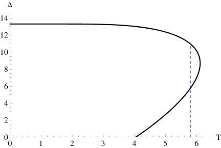
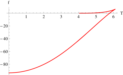
(a)	(b)

Figure 3: a) Temperature dependence of the gap for $b=0.03$, $c=0$, $g\nu=0.3$ and $\omega_{\star}=100$. The condensate forms at $T<T_{c}^{\star}$, $T_{c}^{\star}\approx 5.8$, where the free energy for the upper branch becomes negative. b) The free energy of the lower branch is positive, while it is negative for the upper branch at temperatures $T<T_{c}^{\star}$.

4.3 Combined $\psi^{6}$ and $\psi^{8}$ interactions ($b,\,c\neq 0$)

We now turn on both $b$ and $c$ couplings. For both $b>0$, $c>0$, the picture is qualitatively the same as that for $c=0$. Indeed, as argued in section 3, the $b>0$ term dominates the region near $T_{c}$ and leading to a first order phase transition.

While $T_{c}$ has the same value as the BCS case, $T_{c}^{\star}$ increases as the couplings $b$ and $c$ are increased. Fixing, for instance, $b$, $T_{c}^{\star}$ can be made arbitrarily high by increasing $c$, as shown in fig. 4.

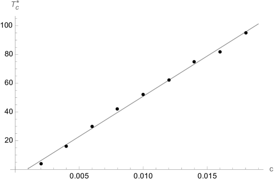
Figure 4: $T_{c}^{\star}$ vs. $c$ for $b=0.001$, $g\nu=0.3$ and $\omega_{\star}=100$. Dots are numerical values, fitted to a straight line.

As the parameter $c$ increases, $\Delta(0)$ also increases. However, the growth of $\Delta(0)$ approaches an asymptotic limit with increasing $c$, as illustrated in fig. 5. To ensure the validity of the regime, where $\Delta(0)\ll\omega_{\star}$ is required, the parameter $g$ must be chosen sufficiently small.

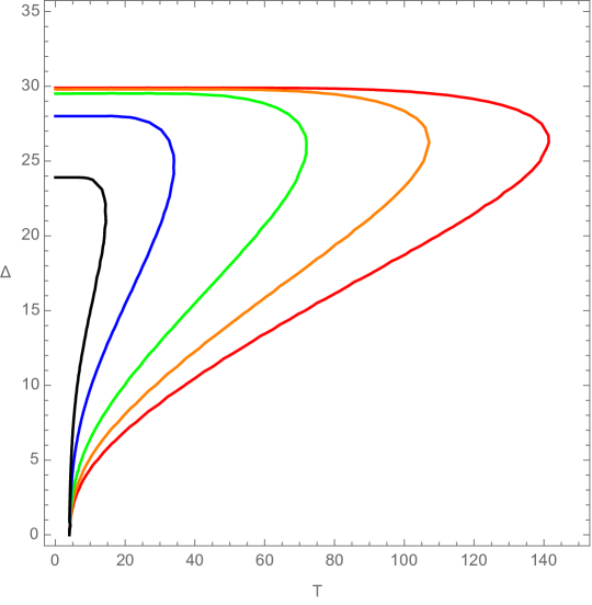
Figure 5: $\Delta$ vs. $T$ for $b=0.001$, $g\nu=0.3$ and $\omega_{\star}=100$ for $c=0.003$ (black), $c=0.005$ (blue), $c=0.010$ (green), $c=0.015$ (orange) and $c=0.020$ (red).

One might consider whether this mechanism could play a role in the behavior of multi-component systems that exhibit high-$T_{c}$ superconductivity. While all known high-$T_{c}$ superconductors display a second-order (continuous) superconducting transition at zero magnetic field, first-order transitions may arise in certain unconventional systems under carefully tuned conditions, such as pressure or doping near a quantum critical point. Clarifying the relevance of such scenarios remains an open question requiring further study.

4.4 The case $b<0$

The case $b<0$ (and $c>0$) exhibits novel features. As discussed in section 3, for negative $b$ the behavior near $T_{c}$ is

$$\Delta\approx\frac{g\nu}{|b|}\,\alpha_{1}\,(T_{c}-T)\,.$$ (4.1)

This behavior indicates a second-order phase transition characterized by a critical exponent of 1 at the critical temperature. Notably, the dynamics is significantly altered depending on the specific values of parameters $|b|$ and $c$. Starting with sufficiently small values $|b|$ and $c$ couplings, the system indeed undergoes a second order phase transition at $T_{c}\approx 4.04$ with critical exponent 1 as shown in fig. 6 (a). However, as the parameter $c$ is increased beyond some critical value, $\Delta$ develops a lump as shown in fig. 6(b).

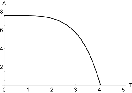
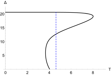
(a)	(b)

Figure 6: $\Delta$ vs. $T$. a) For sufficiently small $|b|$ and $c$, when $b<0$ there is a 2nd order phase transition with critical exponent 1. b) Beyond some critical $c$, the system undergoes a 1st order phase transition at the dashed line, where $\Delta$ jumps from the upper branch to $\Delta=0$.

In this case, as the temperature is decreased, the system first undergoes a first-order phase transition to the upper branch of the $\Delta$ vs. $T$ curve, where $\Delta$ jumps from 0 to a finite value. The lower branches appear as smaller temperatures but they are never thermodynamically relevant because they have larger free energies. This case is qualitatively the same as the $b>0$ case of the previous subsection, but with an additional ingredient. The lowest branch in fig. 6 (b) corresponds to a relative minimum and is therefore locally stable (the free energy in this interval is negative). This indicates the presence of a second-order phase transition in the vicinity of $T_{c}$. However, the thermodynamic behavior is ultimately governed by a more stable extremum of the potential located far in field space, associated with the upper branch of the gap curve. This distant extremum dominates the system’s thermodynamics and drives the onset of a first-order phase transition. Relative minima of the free energy may be relevant as transient states, but they are exponentially suppressed and they do not significantly contribute to the thermodynamics.

For $b<0$, there are regions in $(b,c)$ parameter space that seem to be worth of further exploration. In particular, if $c$ is gradually reduced, one finds a small interval $c_{1}<c<c_{2}$ where the tip of the lump in fig. 6 (b) occurs at a temperature lower than $T_{c}$. As the system is cooled, it would first undergo a second order phase transition with critical exponent 1 followed by a first order phase transition. We leave the characterization of the possible behaviors of the system throughout the parameter space for future work.

5 Conclusions

In this paper we have studied the effect of higher fermion interactions at finite temperature and finite chemical potential in the context of BCS-like phase transitions. While these interactions might be expected to play a minor role, our findings indicate that they can significantly affect the system’s behavior, in some instances modifying the critical exponents or leading to a first-order transition. We have focused on $\psi^{6}$ and $\psi^{8}$ interactions for $N$ non-relativistic fermions coupled to a chemical potential.

When the higher interactions are turned off, the model describes BCS theory with $N$ fermion species and the usual $\psi^{4}$ interaction. In practical applications, models with several species of fermions arise in multiband superconductors [6], where fermions of different bands are treated as different species. Generically, higher fermion interactions may naturally appear in the effective Lagrangian for systems with $N\geq 2$. This suggests that these models might also be relevant in the description of multicomponent (in particular, type 1.5) superconductors (see [4] for a review).

Other potential applications of these models include superconducting systems with strong electron-phonon coupling. These can exhibit deviations from the BCS behavior. The gap curve is typically flatter for most of the temperature range and drops sharply near $T_{c}$ (see e.g. [7]). This is in accordance with the behavior exhibited by the models with $b=0$ and $c<c_{0}$ (black curve in Fig. 1).

For $c>c_{0}$, or for $b>0$, the gap becomes double valued above $T_{c}$. This feature appears in a number of models, in particular, in the Eliashberg-Nambu theory for strong-coupling superconductors [8, 9, 10]. In this parameter range, the present models exhibit a first-order superconducting transition, where the gap edge drops from a finite value to zero. While most common superconductors have a continuous superconducting transition, there are cases where a discontinuous jump in the order parameter is expected. This includes multicomponent superconductors, strong-coupling Eliashberg superconductors and heavy fermions (first-order phase transitions also appear in the presence of magnetic fields).

References

- [1] J. Bardeen, L. N. Cooper and J. R. Schrieffer, “Theory of superconductivity,” Phys. Rev. 108 (1957), 1175-1204.
- [2] J. Polchinski, “Effective field theory and the Fermi surface,” [arXiv:hep-th/9210046 [hep-th]].
- [3] Y. Han, X. Huang, Z. Komargodski, A. Lucas and F. K. Popov, “Entropic Order,” [arXiv:2503.22789 [cond-mat.stat-mech]].
- [4] E. Babaev and J. M. Speight, “Thermodynamically stable non-local vortices, vortex molecules and semi-Meissner state in neither type-I nor type-II multicomponent superconductors,” Phys. Rev. B 72 (2005), 180502 doi:10.1103/PhysRevB.72.180502 [arXiv:cond-mat/0411681 [cond-mat.supr-con]]. E. Babaev, J. Carlström, M. Silaev and J. M. Speight, “Type-1.5 superconductivity in multicomponent systems,” Physica C 533 (2017), 20-35.
- [5] A. Barranco and J. G. Russo, “Supersymmetric BCS,” JHEP 06 (2012), 104 [arXiv:1204.4157 [hep-th]].
- [6] S. P. Kruchinin, “Multiband Superconductors”, Reviews in Theoretical Science, 2016, vol. 4, no 2, p. 165-178.
- [7] R. Khasanov, H. Luetkens, E. Morenzoni, G. Simutis, S. Schönecker, A. Östlin, L. Chioncel and A. Amato, “Superconductivity of Bi-III phase of elemental bismuth: Insights from muon-spin rotation and density functional theory,” Physical Review B 98 (2018), 140504.
- [8] X. H. Zheng and D. G. Walmsley, “Temperature-dependent gap edge in strong-coupling superconductors determined using the Eliashberg-Nambu formalism”, Physical Review B 77 (2008), 104510.
- [9] F. Marsiglio, “Eliashberg Theory: a short review”, Annals of Physics 417 (2020): 168102 [1911.05065].
- [10] F. Marsiglio and J. P. Carbotte. “Electron-phonon superconductivity.” Superconductivity: conventional and unconventional superconductors. Berlin, Heidelberg: Springer Berlin Heidelberg, 2008. 73-162.