Designing lattice spin models and magnon gaps with supercurrents
Abstract
Controlling magnetic interactions at the level of individual spins is relevant for a variety of quantum applications, such as qubits, memory and sensor functionality. Finding ways to exert electrical control over spin interactions, with minimal energy dissipation, is a key objective in this endeavour. We show here that spin lattices and magnon gaps can be controlled with a supercurrent. Remarkably, a spin-polarized supercurrent makes the interaction between magnetic adatoms placed on the surface of a superconductor depend not only on their relative distance, but also on their absolute position in space. This property permits electric control over the interaction not only between two individual spins, but in fact over an entire spin lattice, allowing for non-collinear ground states and a practical arena to study the properties of different spin Hamiltonians. Moreover, we show that a supercurrent controls the magnon gap in antiferromagnetic and altermagnetic insulators. These results provide an accessible way to realize electrically controlled spin switching and magnon gaps without dissipative currents.
Introduction— Electrical control of magnetic interactions is relevant for a variety of quantum applications, such as sensing, computation and memory functionality. Quantum sensing with spin defects Roberts et al. (2025); Fang et al. (2024) does, for example, allow for optically measuring nuclear magnetic resonance (NMR) using the hyperfine magnetic interaction between nuclear spins and spin defects Fang et al. (2024). Quantum computing requires interactions between qubits, such as the magnetic Ruderman–Kittel–Kasuya–Yosida (RKKY) interaction connecting spin qubits Tanamoto and Ono (2021); Yang et al. (2016). Moreover, the Yu-Shiba-Rusinov states that form due to the magnetic interaction between impurity spins and electrons in a superconductor can potentially be used as a qubit Mishra et al. (2021).
The RKKY interaction mediated by electrons in a superconductor provides one promising way of controlling the coupling between impurity spins Nadj-Perge et al. (2014); Pupim and Scheurer (2025); Kim et al. (2018); Heimes et al. (2015); Mohanta et al. (2018); Yazdani et al. (1997); Röntynen and Ojanen (2015). Of particular interest is typically the degree of spin non-collinearity, as this gives rise to interesting spin textures such as spin spirals Kimura (2007); Tokura and Seki (2010), skyrmions Nagaosa and Tokura (2013); Zhang et al. (2020); Marrows and Zeissler (2021) and non-collinear antiferromagnetism Rimmler et al. (2025), all with potential spintronic applications. The ground state configuration of an ensemble of spins can be non-collinear due to a Dzyaloshinskii-Moriya (DM) interaction induced by spin orbit coupling Soumyanarayanan et al. (2016) or from mixed-parity superconductivity with symmetry Ouassou et al. (2025). Another quantity of interest in an ensemble of interacting spins is the magnon energy gap Chumak et al. (2015); Oba et al. (2015); Pradipto et al. (2017); Yoshii et al. (2020); Zhu et al. (2021); Yumnam et al. (2024); Mardele et al. (2024). A tunable magnon gap can, as an example, give rise to a tunable lattice thermal conductivity Vu et al. (2023). The interaction of magnons with superconducting qubits Tabuchi et al. (2015, 2016) and with flux quanta in superconductors Dobrovolskiy et al. (2019); Niedzielski et al. (2023) makes generation, classification and tuning of the magnons possible in superconducting hybrid systems.
In this Letter, we show that supercurrents in superconductors enable electric control over both magnon gaps and magnetic interactions in a way that permits controllable design of a spin lattice. We use second-order perturbation theory to show analytically that a spin supercurrent carried by triplet Cooper pairs gives rise to a number of different interaction terms between magnetic adatoms placed on the superconductor. This causes the ground state configuration of the spins to be non-collinear. Importantly, we find that the ground state depends on the center-of-mass coordinate of the spins. This property allows electric control over the interaction between two spins as illustrated in Fig. 1, and in fact over an entire spin lattice, allowing for the creation of non-collinear ground states that comprise an arena to study the properties of different spin Hamiltonians. Moreover, we demonstrate that when a spin-compensated condensate of spins in the form of an antiferromagnetic or altermagnetic insulator is placed on top of the superconductor, the supercurrent controls the magnitude of the magnon gap. This can be thought of as a dissipationless magnon transistor. The result holds even for a conventional singlet BCS superconductor and occurs already at first order in perturbation theory. The electrical control of a spin lattice and the magnon gap via supercurrents predicted in this Letter reveals a synergy between superconductivity and magnetism that opens new research avenues to explore.
Effective spin-spin interaction—For simplicity, we consider a one-dimensional (1D) superconducting chain with magnetic adatoms placed on its surface Liebhaber et al. (2022). We emphasize that our results carry over to 2D and 3D systems as well. The full Hamiltonian for the system is , where is the Hamiltonian for the superconductor and is the coupling between the magnetic adatoms and the electrons in the superconductor. We consider a superconductor with equal-spin triplet Cooper pairs: this scenario applies both to induced triplet superconductivity via the proximity effect and to an intrinsic triplet superconductor. The former can be achieved by proximitizing an -wave superconductor with one or more ferromagnets Halterman et al. (2007, 2008); Kalcheim et al. (2015) or a conductor with Rashba spin-orbit coupling Reeg and Maslov (2015), or by irradiating an -wave superconductor with light Gassner et al. (2024). The starting point is the attractive Hubbard model in real space,
| (1) |
Here, is the chemical potential, is the hopping constant between nearest neighbors, and is an attractive nearest-neighbor interaction. The operators and creates and destroys, respectively, an electron with spin at lattice site . denotes a sum over nearest-neighbor pairs without double counting. We apply the mean-field approximation to the last term in . The real-space order parameter (OP) is defined as , and to model a supercurrent-carrying state we write it as Takashima et al. (2017)
| (2) |
where and are neighboring lattice sites. Thus, the magnitude does not depend on the positions and themselves. The phase gradient across the material allows for a supercurrent, and is the momentum of the spin– Cooper pairs. If , the supercurrent carries charge and is spin polarized along the spin quantization axis . If , the system carries a pure spin supercurrent. We impose periodic boundary conditions, thus restricting the supercurrent momentum values to where is an integer and is the number of lattice points. The critical momentum is found by solving the gap equation SM . Next, we Fourier transform the electron operators and define the order parameter in –space as . This gives the Hamiltonian up to an irrelevant constant. All -sums run over the crystallographic Brillouin zone. On a 1D lattice with lattice constant , and . The magnitude of the superconducting OP is calculated by solving the gap equation SM , and we choose such that at zero temperature. The coupling term is generally given by
| (3) |
Here, is the coupling strength, is the number of lattice points, and is the Pauli vector. To derive the effective spin-spin interaction, the magnetic adatoms are treated as classical spins at site of the superconductor.
We proceed to diagonalize and perform a Schrieffer-Wolff transformation on . We treat as the perturbation, and average out the fermions in the superconductor to get a pure spin Hamiltonian. The details are provided in SM . For a pure charge or spin supercurrent, there is no coupling between the magnetic adatoms and the superconductor to first order in In this case, the effective spin Hamiltonian is of second order in , and we find it to be
| (4) |
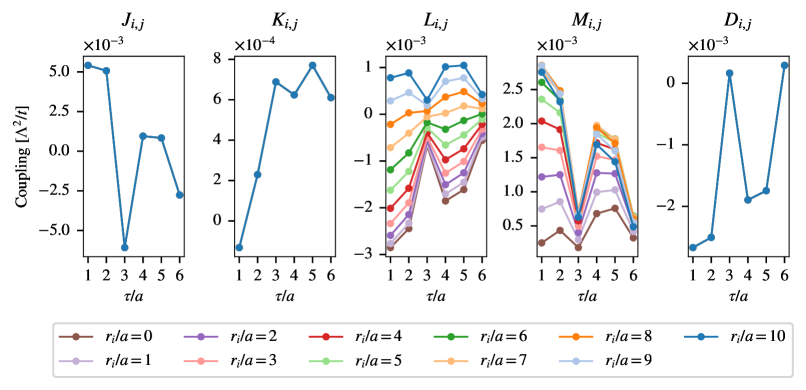
A detailed analytical expression for the coupling constants is given in SM . They all depend on , meaning that the spin-spin interaction can be tuned electrically via the supercurrent. The terms are interpreted as follows. is the exchange coupling, and usually the largest of the coupling constants. It prefers the spins to be aligned in a parallel or antiparallel configuration, depending on its sign. is also an exchange coupling, which tries to align the spins in a parallel or antiparallel configuration along . is a DM interaction that prefers the spin not to be aligned along the same axis. This term is zero in the absence of a spin supercurrent. A positive prefers spins to be aligned along and not along , and oppositely for negative . tries to achieve a misalignment between the spins in the -plane, and it is zero in the absence of a spin supercurrent.
Importantly, and enable the design of a spin lattice via supercurrents. They are given by:
| (5) |
where while the coefficients are large expressions that depend on energy eigenvalues and eigenstates of the superconducting Hamiltonian as well as temperature. Their dependence on the absolute position in the presence of a spin current stands in stark contrast to the conventional relative position dependence that usually appears for RKKY interactions. This is a remarkable feature that arises solely in the presence of a spin supercurrent. It is this dependence that enables the electrical design of a spin lattice, as we will proceed to show. The dependence on absolute position can be understood physically as follows. A Cooper pair of spin electrons with one electron located at and the other electron at has the phase , as seen from Eq. (2). This phase is arbitrary since the physics cannot change under a U(1) gauge transformation of the order parameter. However, phase differences have physical consequences, and in the presence of a spin supercurrent, such a phase difference exists between a Cooper pair with spin and a Cooper pair with spin . This phase difference is , which is precisely the quantity that the spin interaction coefficients depend on.
Electrical tuning of the ground state —Since the magnetic adatoms couple exclusively via the electrons in the superconductor Liebhaber et al. (2022), the ground state configuration is found by minimizing . Note that is invariant under , meaning that the ground state is always twofold degenerate. In the numerical procedure used to calculate the coupling constants in , it is convenient to include a small temperature well below the superconducting critical temperature to effectively turn the Fermi-Dirac distribution functions into slightly smeared step functions. This facilitates numerical convergence and avoids the requirement of computationally infeasible system sizes. We consider below a lattice with sites.
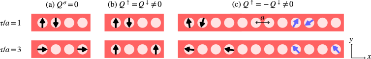
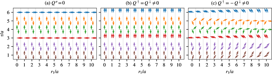
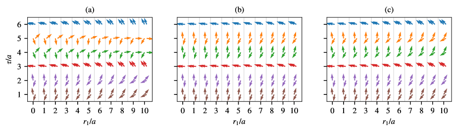
To illustrate how the ground state spin configuration is altered by a supercurrent, we consider two magnetic adatoms and placed on top of a superconductor with equal-spin Cooper pairs. The position of is , and the position of is . Figure 2(a) shows the ground state of these two spins in the absence of a supercurrent for various and values. The ground state configuration can be ferromagnetic or antiferromagnetic, depending on the distance between the spins. Upon applying a charge supercurrent, shown in Fig. 2(b), the spin alignment axis changes for instance from the -plane to the -axis for . Since there is no spin current, the ground state configuration depends on the relative position of the spins , but not on the absolute position of the spins. This changes when the supercurrent is spin-polarized. In Fig. 2(c), a spin supercurrent flows through the superconductor. The onset of non-zero and causes the spins to be non-collinear, and the angle difference from a collinear state is up to 65 degrees. Moreover, the ground state configuration now depends on the absolute position of the spins in the lattice. This enables the possibility to design a lattice spin model that breaks translational invariance. We have verified that these properties are robust upon varying the chemical potential SM .
Magnon gap—
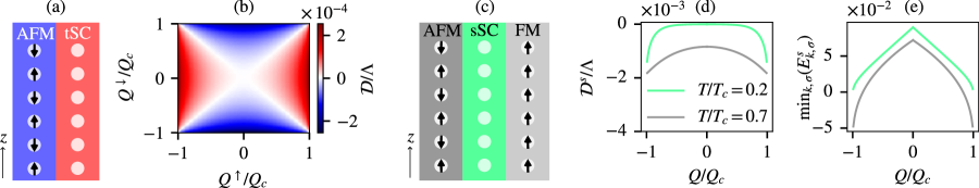
We now replace the two impurity spins considered up to now with an entire spin condensate that is proximity-coupled to a superconductor to demonstrate a new effect: electric control of a magnon gap in a spin-compensated magnet via a supercurrent. Consider a bilayer consisting of an antiferromagnetic insulator and a superconductor with equal-spin Cooper pairs relative to the Néel order, as illustrated in Fig. 3(a). The first order contribution to the magnon gap in the antiferromagnetic insulator is found by calculating where are the fermionic operators that diagonalize , applying the Holstein-Primakoff transformation to the spin operators, and diagonalizing the full Hamiltonian for the antiferromagnetic insulator. We find that is equivalent to an applied magnetic field, and the analytical supercurrent-induced contribution to the magnon gap is
| (6) |
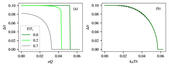
where is the Fermi-Dirac distribution. The calculation details as well as definitions of the eigenenergy and the coherence factors and are provided in SM . A pure charge supercurrent or a pure spin supercurrent gives , while any combination of a charge and spin supercurrent gives a tunable . This is shown in Fig. 3(b). In other words, a spin-polarized supercurrent tunes the magnitude of the magnon gap. When , the magnon gap is enhanced for one magnon species and suppressed for the other magnon species.
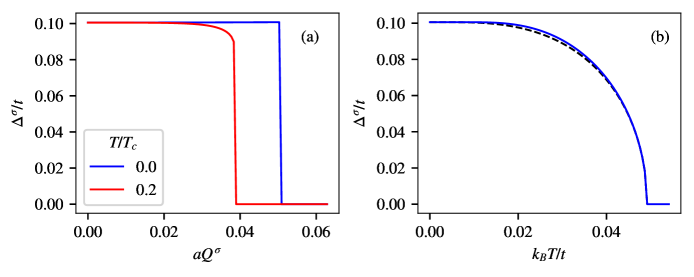
Interestingly, there may exist an even simpler way to control magnon gaps in antiferromagnetic insulators experimentally. Consider a bilayer consisting of a thin-film conventional -wave superconductor with a spin-splitting field and an antiferromagnetic insulator on top, as illustrated in Fig. 3(c). The spin-splitting field in the superconductor can be achieved either via an applied in-plane external field or by proximity to a ferromagnet underneath the superconductor. The supercurrent-induced contribution to the magnon gap is analytically computed to be SM :
| (7) |
The supercurrent-induced magnon gap against the Cooper pair momentum is shown in Fig. 3(d). The momentum is spin-independent because the Cooper pairs consist of electrons with opposite spins, and they cannot carry a spin current. Nevertheless, the charge supercurrent in this case controls the magnitude of the magnon gap. The physics can be understood as follows. The spin splitting field induces a spin imbalance in the superconductor, which couples to the magnon density. The spin imbalance is determined by the excitation spectrum in the superconductor, which is altered when applying a supercurrent. The gap in the energy dispersion decreases for increasing , as shown in Fig. 3(e). When the gap decreases, it becomes easier to excite quasiparticles, and their spin imbalance alters the magnon gap. This also explains why the supercurrent-induced magnon gap is larger at compared to . In this way, electrical tuning of the magnon gap via a supercurrent is realized using conventional superconductivity. A possible material setup to measure this effect is a EuS/Nb bilayer with either an insulating antiferromagnet (Fe2O3) or altermagnet (MnTe) grown on top. A supercurrent flow can also influence the magnon gap and electron density of states in a superconductor/ferromagnet structure Johnsen et al. (2021); Ianovskaia et al. (2023).
The fact that the intrinsic magnon gap in the antiferromagnetic insulator is enhanced by supercurrent for one magnon species but suppressed for the other lifts their degeneracy. Interestingly, this is the key to inducing magnon spin currents in antiferromagnets via for instance the spin Seebeck effect Rezende et al. (2019).
Our results thus demonstrate a route to electrically tunable magnon spin currents in antiferromagnetic insulators, controlled by a dissipationless supercurrent. With regard to the magnitude of the supercurrent-induced magnon gap, our approach is perturbative in nature and thus only small modifications of the magnon gap are within the regime of validity of our methodology. However, a non-perturbative approach using stronger coupling would very likely increase this magnitude, and thus experiments probing this effect in bilayers of superconductors and antiferromagnets with good interfacial coupling would be of high interest. Finally, we underline that our results apply to an altermagnetic insulator as well by generalizing the model to 2D.
Summarizing, we predict that charge and spin supercurrents in superconductors enable electric control over both magnon gaps and magnetic interactions in a way that permits controllable designing of a spin lattice. This reveals a synergy between superconductivity and magnetism that opens up a research avenue with relevance to applications where spin interactions are the key ingredient.
Acknowledgements.
This work was supported by the Research Council of Norway through Grant No. 323766 and its Centres of Excellence funding scheme Grant No. 262633 “QuSpin.” The numerical calculations were performed on resources provided by Sigma2—the National Infrastructure for High Performance Computing and Data Storage in Norway, project NN9577K.References
- Roberts et al. (2025) H. Roberts, H. Abudayyeh, X. Li, and X. Li, “Quantum Sensing with Spin Defects Beyond Diamond,” ACS Nano (2025).
- Fang et al. (2024) H.-H. Fang, X.-J. Wang, X. Marie, and H.-B. Sun, “Quantum sensing with optically accessible spin defects in van der Waals layered materials,” Light: Science & Applications 13, 303 (2024).
- Tanamoto and Ono (2021) T. Tanamoto and K. Ono, “Compact spin qubits using the common gate structure of fin field-effect transistors,” AIP Advances 11 (2021).
- Yang et al. (2016) G. Yang, C.-H. Hsu, P. Stano, J. Klinovaja, and D. Loss, “Long-distance entanglement of spin qubits via quantum Hall edge states,” Physical Review B 93, 075301 (2016).
- Mishra et al. (2021) A. Mishra, P. Simon, T. Hyart, and M. Trif, “Yu-Shiba-Rusinov qubit,” PRX Quantum 2, 040347 (2021).
- Nadj-Perge et al. (2014) S. Nadj-Perge, I. K. Drozdov, J. Li, H. Chen, S. Jeon, J. Seo, A. H. MacDonald, B. A. Bernevig, and A. Yazdani, “Observation of Majorana fermions in ferromagnetic atomic chains on a superconductor,” Science 346, 602–607 (2014).
- Pupim and Scheurer (2025) L. V. Pupim and M. S. Scheurer, “Adatom engineering magnetic order in superconductors: Applications to altermagnetic superconductivity,” Physical Review Letters 134, 146001 (2025).
- Kim et al. (2018) H. Kim, A. Palacio-Morales, T. Posske, L. Rózsa, K. Palotás, L. Szunyogh, M. Thorwart, and R. Wiesendanger, “Toward tailoring Majorana bound states in artificially constructed magnetic atom chains on elemental superconductors,” Science Advances 4, eaar5251 (2018).
- Heimes et al. (2015) A. Heimes, D. Mendler, and P. Kotetes, “Interplay of topological phases in magnetic adatom-chains on top of a Rashba superconducting surface,” New Journal of Physics 17, 023051 (2015).
- Mohanta et al. (2018) N. Mohanta, A. P. Kampf, and T. Kopp, “Supercurrent as a probe for topological superconductivity in magnetic adatom chains,” Physical Review B 97, 214507 (2018).
- Yazdani et al. (1997) A. Yazdani, B. A. Jones, C. P. Lutz, M. F. Crommie, and D. M. Eigler, “Probing the local effects of magnetic impurities on superconductivity,” Science 275, 1767–1770 (1997).
- Röntynen and Ojanen (2015) J. Röntynen and T. Ojanen, “Topological superconductivity and high Chern numbers in 2D ferromagnetic Shiba lattices,” Physical Review Letters 114, 236803 (2015).
- Kimura (2007) T. Kimura, “Spiral magnets as magnetoelectrics,” Annu. Rev. Mater. Res. 37, 387–413 (2007).
- Tokura and Seki (2010) Y. Tokura and S. Seki, “Multiferroics with spiral spin orders,” Advanced Materials 22, 1554–1565 (2010).
- Nagaosa and Tokura (2013) N. Nagaosa and Y. Tokura, “Topological properties and dynamics of magnetic skyrmions,” Nature Nanotechnology 8, 899–911 (2013).
- Zhang et al. (2020) X. Zhang, Y. Zhou, K. M. Song, T.-E. Park, J. Xia, M. Ezawa, X. Liu, W. Zhao, G. Zhao, and S. Woo, “Skyrmion-electronics: writing, deleting, reading and processing magnetic skyrmions toward spintronic applications,” Journal of Physics: Condensed Matter 32, 143001 (2020).
- Marrows and Zeissler (2021) C. H. Marrows and K. Zeissler, “Perspective on skyrmion spintronics,” Applied Physics Letters 119 (2021).
- Rimmler et al. (2025) B. H. Rimmler, B. Pal, and S. S. P. Parkin, “Non-collinear antiferromagnetic spintronics,” Nature Reviews Materials 10, 109–127 (2025).
- Soumyanarayanan et al. (2016) A. Soumyanarayanan, N. Reyren, A. Fert, and C. Panagopoulos, “Emergent phenomena induced by spin–orbit coupling at surfaces and interfaces,” Nature 539, 509–517 (2016).
- Ouassou et al. (2025) J. A. Ouassou, T. Yokoyama, and J. Linder, “Dzyaloshinskii-Moriya-type spin-spin interaction from mixed-parity superconductivity,” Physical Review B 111, L060504 (2025).
- Chumak et al. (2015) A. V. Chumak, V. I. Vasyuchka, A. A. Serga, and B. Hillebrands, “Magnon spintronics,” Nature Physics 11, 453–461 (2015).
- Oba et al. (2015) M. Oba, K. Nakamura, T. Akiyama, T. Ito, M. Weinert, and A. J. Freeman, “Electric-field-induced modification of the magnon energy, exchange interaction, and Curie temperature of transition-metal thin films,” Physical Review Letters 114, 107202 (2015).
- Pradipto et al. (2017) A.-M. Pradipto, T. Akiyama, T. Ito, and K. Nakamura, “Mechanism and electric field induced modification of magnetic exchange stiffness in transition metal thin films on MgO (001),” Physical Review B 96, 014425 (2017).
- Yoshii et al. (2020) S. Yoshii, R. Ohshima, Y. Ando, T. Shinjo, and M. Shiraishi, “Detection of ferromagnetic resonance from 1 nm-thick Co,” Scientific Reports 10, 15764 (2020).
- Zhu et al. (2021) F. Zhu, L. Zhang, X. Wang, F. J. Dos Santos, J. Song, T. Mueller, K. Schmalzl, W. F. Schmidt, A. Ivanov, J. T. Park, et al., “Topological magnon insulators in two-dimensional van der Waals ferromagnets CrSiTe3 and CrGeTe3: Toward intrinsic gap-tunability,” Science Advances 7, eabi7532 (2021).
- Yumnam et al. (2024) G. Yumnam, D. H. Moseley, J. A. M. Paddison, C. Z. Suggs, E. Zappala, D. S. Parker, G. E. Granroth, G. D. Morris, M. M. H. Polash, D. Vashaee, et al., “Magnon gap tuning in lithium-doped MnTe,” Physical Review B 109, 214434 (2024).
- Mardele et al. (2024) F. L. Mardele, I. Mohelsky, D. Jana, A. Pawbake, J. Dzian, W.-L. Lee, K. Raju, R. Sankar, C. Faugeras, M. Potemski, et al., “Tuning THz magnons in a mixed van-der-Waals antiferromagnet,” arXiv preprint arXiv:2408.12230 (2024).
- Vu et al. (2023) D. D. Vu, R. A. Nelson, B. L. Wooten, J. Barker, J. E. Goldberger, and J. P. Heremans, “Magnon gap mediated lattice thermal conductivity in MnBi2Te4,” Physical Review B 108, 144402 (2023).
- Tabuchi et al. (2015) Y. Tabuchi, S. Ishino, A. Noguchi, T. Ishikawa, R. Yamazaki, K. Usami, and Y. Nakamura, “Coherent coupling between a ferromagnetic magnon and a superconducting qubit,” Science 349, 405–408 (2015).
- Tabuchi et al. (2016) Y. Tabuchi, S. Ishino, A. Noguchi, T. Ishikawa, R. Yamazaki, K. Usami, and Y. Nakamura, “Quantum magnonics: The magnon meets the superconducting qubit,” Comptes Rendus. Physique 17, 729–739 (2016).
- Dobrovolskiy et al. (2019) O. V. Dobrovolskiy, R. Sachser, T. Brächer, T. Böttcher, V. V. Kruglyak, R. V. Vovk, V. A. Shklovskij, M. Huth, B. Hillebrands, and A. V. Chumak, “Magnon–fluxon interaction in a ferromagnet/superconductor heterostructure,” Nature Physics 15, 477–482 (2019).
- Niedzielski et al. (2023) B. Niedzielski, C. L. Jia, and J. Berakdar, “Magnon-fluxon interaction in coupled superconductor/ferromagnet hybrid periodic structures,” Physical Review Applied 19, 024073 (2023).
- Liebhaber et al. (2022) E. Liebhaber, L. M. Rütten, G. Reecht, J. F. Steiner, S. Rohlf, K. Rossnagel, F. von Oppen, and K. J. Franke, “Quantum spins and hybridization in artificially-constructed chains of magnetic adatoms on a superconductor,” Nature Communications 13, 2160 (2022).
- Halterman et al. (2007) K. Halterman, P. H. Barsic, and O. T. Valls, “Odd triplet pairing in clean superconductor/ferromagnet heterostructures,” Physical Review Letters 99, 127002 (2007).
- Halterman et al. (2008) K. Halterman, O. T. Valls, and P. H. Barsic, “Induced triplet pairing in clean -wave superconductor/ferromagnet layered structures,” Physical Review B—Condensed Matter and Materials Physics 77, 174511 (2008).
- Kalcheim et al. (2015) Y. Kalcheim, O. Millo, A. Di Bernardo, A. Pal, and J. W. A. Robinson, “Inverse proximity effect at superconductor-ferromagnet interfaces: Evidence for induced triplet pairing in the superconductor,” Physical Review B 92, 060501 (2015).
- Reeg and Maslov (2015) C. R. Reeg and D. L. Maslov, “Proximity-induced triplet superconductivity in Rashba materials,” Physical Review B 92, 134512 (2015).
- Gassner et al. (2024) S. Gassner, C. S. Weber, and M. Claassen, “Light-induced switching between singlet and triplet superconducting states,” Nature Communications 15, 1776 (2024).
- Takashima et al. (2017) R. Takashima, S. Fujimoto, and T. Yokoyama, “Adiabatic and nonadiabatic spin torques induced by a spin-triplet supercurrent,” Physical Review B 96, 121203(R) (2017).
- (40) See Supplementary Material, including references Hodt and Linder (2024); Gross et al. (1986); Tinkham (2004), at URL to be inserted for the derivation details of the effective spin-spin interaction, the numerical method for determining the ground state configuration, derivation details for the supercurrent-induced magnon gap, and the gap equation for the superconducting order parameter.
- Johnsen et al. (2021) L. G. Johnsen, H. T. Simensen, A. Brataas, and J. Linder, “Magnon spin current induced by triplet Cooper pair supercurrents,” Physical Review Letters 127, 207001 (2021).
- Ianovskaia et al. (2023) A. S. Ianovskaia, A. M. Bobkov, and I. V. Bobkova, “Magnon influence on the superconducting density of states in superconductor–ferromagnetic-insulator bilayers,” Phys. Rev. B 108, 214501 (2023).
- Rezende et al. (2019) S. M. Rezende, A. Azevedo, and R. L. Rodríguez-Suárez, “Introduction to antiferromagnetic magnons,” Journal of Applied Physics 126, 151101 (2019).
- Hodt and Linder (2024) E. W. Hodt and J. Linder, “Spin pumping in an altermagnet/normal-metal bilayer,” Physical Review B 109, 174438 (2024).
- Gross et al. (1986) F. Gross, B. S. Chandrasekhar, D. Einzel, K. Andres, P. J. Hirschfeld, H. R. Ott, J. Beuers, Z. Fisk, and J. L. Smith, “Anomalous temperature dependence of the magnetic field penetration depth in superconducting UBe13,” Zeitschrift für Physik B Condensed Matter 64, 175–188 (1986).
- Tinkham (2004) M. Tinkham, Introduction to Superconductivity (Dover Books on Physics Series, Dover, New York, 2004).
- Sigrist (2005) M. Sigrist, “Introduction to unconventional superconductivity,” AIP Conference Proceedings, 789, 165–243 (2005).
Supplemental material
Johanne Bratland Tjernshaugen1, Martin Tang Bruland1, and Jacob Linder1
1Center for Quantum Spintronics, Department of Physics, Norwegian
University of Science and Technology, NO-7491 Trondheim, Norway
I Derivation of the effective spin-spin interaction
I.1 Diagonalizing the Hamiltonian
The mean-field Hamiltonian for a triplet superconductor with equal-spin Cooper pairs is
| (S1) |
Here, runs through the crystallographic Brillouin zone (BZ). From this point, we implicitly assume that all - and -sums run over the crystallographic Brillouin zone except if stated otherwise and we write instead of . By introducing the basis , the Hamiltonian becomes
| (S2) |
Diagonalization is achieved through the Bogoliubov transformation
| (S3) |
where for the -operators to be fermionic, and and for the transformation to be consistent. The diagonalized Hamiltonian is . This gives the coherence factors
| (S4) |
and the eigenvalues
| (S5) |
For later convenience, we define .
I.2 Effective spin-spin interaction
The coupling between the itinerant electrons and the classical spins is given by
| (S6) |
The goal is to perform a Schrieffer-Wolff transformation to get an effective spin model. The full Hamiltonian is , where we treat as a perturbation. Note that diagonal elements of the perturbation should be absorbed into in order to allow for first-order contributions in the transformed Hamiltonian. In other words, if , these terms should be included in . is calculated in Eq. (S17), and in the presence of a pure charge or spin supercurrent, this term is zero. For a spin-polarized charge supercurrent, the first-order term, which is effectively a magnetic field, will dominate the spin Hamiltonian. From here on, we assume that the interaction between the magnetic adatoms is induced by a pure charge or spin supercurrent, and we calculate the spin-spin interaction to second order in . The Hamiltonian is canonically transformed to , where is a hermitian operator known as a generator. This transformed Hamiltonian has the same spectrum as the original Hamiltonian. If the generator is chosen such that , the transformed Hamiltonian is up to second order in . The effective spin Hamiltonian is found by integrating out the –fermions that diagonalize :
| (S7) |
The first step is to find a generator such that is satisfied. The coupling term is rewritten in terms of the operators,
| (S8) |
and the ansatz generator has the same form but with different prefactors,
| (S9) |
The prefactors are determined by comparing the left-hand side of the equation to the right-hand side. This gives expressions of the kind
| (S10) |
The right-hand side of this equation is in general nonzero, even when . This is resolved by letting diverge such that the equality is satisfied. In the final expression for the Hamiltonian, always shows up in combination with Fermi-Dirac distributions. This gives a derivative of the Fermi-Dirac distribution as :
| (S11) |
where is the Fermi-Dirac distribution at temperature and .
The next step is to average out the –fermions. The average , and
| (S12) |
We find the effective contribution to the interaction between the spins,
| (S13) |
The coupling constants are defined in Table 1.
| Quantity | Definition | Properties |
|---|---|---|
| - | ||
| when | ||
| , and when | ||
I.3 Numerical calculation of the coupling constants
The coupling constants are calculated on a lattice with lattice points. We have confirmed that this size is sufficient for the coefficients to converge. The exception is when the magnitude of the superconducting OP is small, because then the derivative of the Fermi-Dirac distribution is spiky and a larger number of lattice points is required.
The coupling constants belonging to Fig. 1(c) and 2(c) in the main text are shown in Fig. S1. We observe that the coupling strength generally decreases when the distance increases. is an order of magnitude greater than the other coupling constants, and wants the spins to be aligned in a collinear configuration. The coupling constants and depend on the absolute position of the spins. The coupling constants in Fig. S1 are used to calculate the ground state configuration. Similar calculations were performed to calculate the coupling constants for the other parameter configurations for which we calculate the ground state.
II Calculating the ground state configuration
The ground state configuration of the spins is found by minimizing . Upon increasing the temperature, the probability for the system to be in any spin configuration is given by the Boltzmann factor , where is the partition function. Since our effective Hamiltonian is derived using perturbation theory, the coupling constant and thus are small. Therefore, at a finite temperature that exceeds the magnitude of the highest excited state of the Hamiltonian, all spin configurations are sampled in the partition function. However, a non-perturbative approach would in all likelihood yield larger coefficients in , indicating that the spins would stay close to their ground state configuration upon increasing the temperature, thus allowing for the possibility to design a spin lattice at finite temperature. In other words, the stronger the coupling, the more robust the ground state spin configuration against thermal fluctuations.
The first step in calculating the ground state configuration is to calculate the coefficients in at zero temperature. It is convenient to include a small temperature in the numerical procedure used to calculate the coupling constants in Eq. (S13), because this effectively turns the Fermi-Dirac distribution functions into slightly smeared step functions. When the coupling constants are calculated, it is possible to calculate the ground state of the spins. To demonstrate how the ground state is altered by the supercurrent, we consider two spins and placed on the superconductor. The spins can take the values
| (S14) |
The ground state configuration is found ”brute force” by calculating for equally spaced values for and equally spaced values for , and finding the configuration that gives the lowest value for . This gives in total combinations for the spins and . gives a 1 degree uncertainty, and this is the value we have used when determining the ground state.
The ground state configuration remains non-collinear and center-of-mass dependent, as in the main manuscript, when the chemical potential is increased or when the spin current magnitude is decreased. This is shown in Fig. S2.
Upon decreasing the magnitude of the superconducting OP, the coupling constant becomes dominant and the ground state configuration becomes approximately collinear without specific preferences for the axis alignment.
III Magnon gap
III.1 Equal spin pairing
The first-order contribution to the magnon spectrum is found by calculating
| (S15) |
where denote the sublattices of the antiferromagnet. We assume for simplicity that the -coupling strength is the same for both sublattices. For a superconductor with equal-spin Cooper pairs, the coherence factors and that diagonalize the Hamiltonian are given in Eq. (S4). The corresponding eigenvalues are given in Eq. (S5). Rewriting the –operators in terms of the –operators according to Eq. (S3) and taking the average over the –operators gives
| (S16) |
The effective contribution to the spin Hamiltonian is
| (S17) |
with
| (S18) |
This is effectively an applied magnetic field in the -direction. This connection can also be seen directly by calculating the magnetization in the superconductor,
| (S19) |
The physical interpretation is that when the spin- Cooper pairs gain a momentum , the occupation of the spin- quasiparticles changes and the superconductor gains a net magnetization. The magnetization is independent of the sign of the Cooper pair momentum .
The magnon gap is found by diagonalizing the following Hamiltonian, which, depending on the interaction parameter choices, can model either a conventional antiferromagnet or altermagnet Hodt and Linder (2024):
| (S20) |
The model is illustrated in Fig. S3. denotes the pairs of next-nearest neighbors connected along the -direction within the sublattice. This altermagnetic model consists of two superimposed square lattices, where the interactions are a nearest-neighbor interaction , an anisotropic next-nearest-neighbor interaction which is rotated for one sublattice compared to the other, and an anisotropy term . A pure antiferromagnetic model is achieved by setting .
We apply the Holstein-Primakoff transformation to the spin operators on each sublattice:
| (S21) |
We then Fourier transform and and find
| (S22) |
where MBZ is the magnetic Brillouin zone, , , and . The Hamiltonian is diagonalized through the Bogoliubov transformation
| (S23) |
and for the new operators to be bosonic. The diagonalized Hamiltonian becomes
| (S24) |
with eigenvalues
| (S25) |
and coherence factors
| (S26) |
Here, and . We see that the eigenvalues are and , where and do not depend on the supercurrent. This shows that is the contribution to the magnon gap from the supercurrent, and that the magnon gap is enhanced for magnon species and suppressed for magnon species when .
If the triplet superconducting OP , the magnon gap correction is zero in the presence of a pure charge supercurrent or a pure spin supercurrent. For the charge current , the absolute value of the coherence factors in Eq. (S4) and the eigenenergies in Eq. (S5) are spin independent. Therefore, the spin sum in Eq. (S18) is zero. For a pure spin supercurrent , we use that . Again, we find that the absolute value of the coherence factors in Eq. (S4) are spin independent, and the eigenenergy . Since and , we find again that the spin sum and thus is zero. A non-zero is thus obtained for a spin-polarized charge supercurrent ().
III.2 Spin singlet -wave Cooper pairs
The Hubbard Hamiltonian in real space for a spin-split spin singlet -wave superconductor is
| (S27) |
Here, is the spin splitting. We apply the mean-field approximation to the last term in . The real-space order parameter is defined as , and we assume that it is an -wave superconductor and the OP takes the form
| (S28) |
The momentum of the Cooper pairs is now spin-independent. Next, we Fourier transform the electron operators. This gives the Hamiltonian
| (S29) |
up to a constant. The superconducting OP satisfies . In the basis , the Hamiltonian is
| (S30) |
Diagonalization is achieved through the Bogoliubov transformation
| (S31) |
where for the -operators to be fermionic, and and for the transformation to be consistent. The diagonalized Hamiltonian is . This gives the coherence factors
| (S32) |
and the eigenvalues
| (S33) |
This gives, as before, magnon energies , where and do not depend on the supercurrent. The magnon gap correction is
| (S34) |
The magnitudes of the coherence factors are spin independent and the eigenenergy depends on spin only through the spin splitting field. Therefore, a non-zero spin splitting is required to achieve a nonzero magnon gap correction. The magnon gap correction can be simplified by shifting and relabeling in the sum over the –term:
| (S35) |
IV Gap equation for the superconducting order parameter
In the numerical calculation of the coupling constants in Eq. (S13), we assumed that the magnitude of the superconducting OP was independent of the applied supercurrent. This is justified in this section. Moreover, when we calculated the supercurrent-induced contribution to the magnon gap, we assumed that the magnitude of the superconducting OP at , and in the absence of any supercurrents was . At finite temperature, the magnitude of the OP is reduced and depends on the supercurrent, and it is calculated by solving the gap equation.
IV.1 Equal spin pairing
The superconducting order parameter is defined as , where and are nearest neighbors. Moreover, the OP in -space was defined as . Note that we keep the spin dependence of the OP here for generality. Rearranging the above definitions gives
| (S36) |
We Fourier transform the electron operators and perform a sum over all lattice points to remove the -dependence. This gives
| (S37) |
The electron operators are replaced with -operators according to Eq. (S3). The gap equation becomes
| (S38) |
Figure S4(a) shows the -dependence of the OP magnitude. Below the critical current, it is reasonable to approximate the gap as -independent. Therefore, it is reasonable to approximate the OP magnitude as spin independent since the OP magnitude depends on spin only through the Cooper pair momentum . The critical Cooper pair momentum is at and at . Here, is the critical temperature when , as shown in Fig. S4(b). The supercurrent magnitude used in Fig. 1 and 2 in the main text is below the critical supercurrent at .
As for realistic materials, a critical current is quite large. Take for example NbTi, which is a type II superconductor known to have a high critical current. The critical current is given by , and the BCS coherence length is This gives Tinkham (2004). The coherence length of NbTi is , which gives . Even though the superconducting OP magnitude and critical current we use are large, we argue that it is reasonable to use these values. The effects predicted by second-order perturbation theory are expected to be small, and using a large OP and critical current is a way of allowing the effects to be larger even within the perturbative approach.
IV.2 Spin singlet -wave Cooper pairs
The superconducting OP for a spin singlet -wave superconductor is defined as
| (S39) |
We Fourier transform the electron operators, and the gap equation takes the form
| (S40) |
The -dependence on the right-hand side is removed by performing the sum on both sides. This gives
| (S41) |
We use the transformation in Eq. (S31) and find
| (S42) |
Inserting the coherence factors gives
| (S43) |