Color field configuration between three static quarks

Abstract

Within Yang-Mills-Proca theory with external sources, regular, finite energy solutions are obtained. It is shown that color electric/magnetic fields have two components: the first part is a gradient/curl component, respectively, and the second part is a nonlinear component. It is shown that the color electric field has a Y-like spatial distribution. Such a Y-like behavior arises because the gradient component of the electric field is present. The nonlinear component of the electric field is a curl one, and it appears because the vector potential sourced by a solenoidal current is present. The color magnetic field is purely curl one, since its nonzero color components do not contain a nonlinear component; this results in the fact that its force lines lie on the surface of a torus. It is shown that the results obtained are in good agreement with the results obtained in lattice calculations in quantum chromodynamics. To discuss such an agreement, we consider a procedure of nonperturbative quantization and discuss possible approximations ensuring such an agreement. Also, we compare the energy profile obtained by us with that obtained in lattice calculations with a static potential.

I Introduction

At the present time lattice calculations in nonperturbative quantum chromodynamics (QCD) have achieved a great success (see, e.g., the reviews [1, 2, 3] and references therein). Considerable results have been obtained: (a) a comparison of perturbative global PDF analyses and the lattice QCD calculations was carried out; (b) QCD calculations on the thermodynamics of strong-interaction matter were performed; (c) the QCD phase transition was investigated; (d) an equation of state was proposed, etc.

In Ref. [4], within lattice QCD, the nucleon spin carried by valence and sea quarks and gluons is determined. Refs. [5, 6] study the distribution of a field between two quarks and show that a color electric field created by these quarks is confined in a flux tube. The papers [7, 8, 9] study the distribution of quantum SU(3) gauge fields created by three static quarks.

In lattice calculations (see, e.g., Ref. [7]), it is shown that, in QCD, there are well-ordered distributions of color electric and magnetic fields creating $\Delta$- and Y-like distributions of the color electric field. This suggests that there can exist differential equations describing such distributions. Searching for such equations is, of course, a quite complicated problem. One may assume that such equations must follow from the quantum Yang-Mills equations in the process of nonperturbative quantization as some approximation for such quantization.

At the present time Proca theories (massive Yang-Mills theories) are under quite active investigation. For example, Refs. [10, 11, 12, 13] study gravitating Proca fields, for which regular solutions are obtained. In Refs. [14, 15] the cosmological implications of generalized Proca theories are investigated. The paper [16] studies static and spherically symmetric solutions in the class of generalized Proca theories with non-minimal coupling to the Einstein tensor.

Our purpose here is to investigate a distribution of SU(3) non-Abelian field within Yang-Mills-Proca theory with external sources (see Fig. 1): (a) quarks located at the vertices of an equilateral triangle $ABC$ which create a Y-like distribution of a color electric field; (b) color charges distributed along the sides of this triangle which are needed for the existence of a nonlinear component of such electric field; (c) toroidal currents (shown in Fig. 1) which are necessary for the appearance of a color vector potential whose presence, in turn, results in the appearance of a curl component of the electric field.

Figure 1: A sketch of distribution of static quarks and charge/current densities creating color electric, $\vec{E}^{a}$, and magnetic, $\vec{H}^{a}$, fields.

We wish to show that Yang-Mills-Proca theory enables one to obtain a fairly well agreement with the results obtained in lattice calculations in QCD. This means that such theory may be regarded as some approximation for the procedure of nonperturbative quantization in QCD. In such case, there arises an interesting question of what physical approximations must be done in this procedure to derive Yang-Mills-Proca theory. To clarify this question, we consider the procedure of nonperturbative quantization suggested by W. Heisenberg in Ref. [17] and developed in Refs. [18, 19, 20] and discuss what approximations must be done to obtain necessary nonperturbative quantum corrections leading to the required result.

II Starting Lagrangian and equations

The Lagrangian describing a system consisting of a non-Abelian SU(3) Proca field $A^{a}_{\mu}$ sourced by color charges and currents can be taken in the form (hereafter, we work in natural units $c=\hbar=1$)

$$\mathcal{L}=-\frac{1}{4}F^{a}_{\mu\nu}F^{a\mu\nu}+\frac{m^{2}}{2}A^{a}_{\mu}A^{a\mu}-A^{a}_{\mu}j^{a\mu}.$$ (1)

Here $F^{a}_{\mu\nu}=\partial_{\mu}A^{a}_{\nu}-\partial_{\nu}A^{a}_{\mu}+gf_{abc}A^{b}_{\mu}A^{c}_{\nu}$ is the field strength tensor for the Proca field of mass $m$, where $f_{abc}$ are the SU(3) structure constants; $g$ is the coupling constant; $j^{a\mu}=\left\{j^{at},-\vec{j}^{\,a}\right\}$ are color four-currents; $a,b,c=1,2,\dots,8$ are color indices; $\mu,\nu=0,1,2,3$ are spacetime indices.

Using (1), the corresponding field equations can be written in the form

$$D_{\nu}F^{a\mu\nu}-m^{2}A^{a\mu}\equiv\frac{1}{\sqrt{-\mathcal{G}}}\frac{\partial}{\partial x^{\nu}}\left(\sqrt{-\mathcal{G}}F^{a\mu\nu}\right)+gf_{abc}A^{b}_{\nu}F^{c\mu\nu}-m^{2}A^{a\mu}=-j^{a\mu},$$ (2)

where $\mathcal{G}$ is the determinant of the spacetime metric and the energy density is

$$\begin{split}\varepsilon=&\frac{1}{2}\left(E^{a}_{i}\right)^{2}+\frac{1}{2}\left(H^{a}_{i}\right)^{2}+m^{2}\left(A^{a0}A^{a}_{0}-\frac{1}{2}A^{a}_{\alpha}A^{a\alpha}\right),\end{split}$$ (3)

where $i=1,2,3$ and $E^{a}_{i}$ and $H^{a}_{i}$ are the components of the color electric and magnetic field strengths, respectively.

To find the SU(3) non-Abelian field in Yang-Mills-Proca theory, we employ the following ansatz in Cartesian coordinates:

$$\begin{split}A^{a}_{\mu}=&\frac{1}{g}\left\{h^{a},v^{a},u^{a},w^{a}\right\},\quad a=3,6,7,8,\\ A^{n}_{\mu}=&0,\quad n=1,2,4,5,\end{split}$$ (4)

where $h^{a},v^{a},u^{a},$ and $w^{a}$ are functions of $x,y,z$ and $A^{a}_{\mu}$ belongs to the subgroup of SU(3).

For these potentials, we have the following color electric, $\vec{E}^{a}$, and magnetic, $\vec{H}^{a}$, fields:

$$E^{a}_{i}= -\frac{1}{g}\left(\gradient{h^{a}}\right)_{i}+gf_{abc}A^{b}_{t}A^{c}_{i},$$ (5)

$$H^{a}_{i}= \left(\curl{\vec{A}^{a}}\right)_{i}+gf_{abc}\epsilon_{ijk}A^{b}_{j}A^{c}_{k}=\left(\curl{\vec{A}^{a}}\right)_{i}+gf_{abc}\left[\vec{A}^{b}\times\vec{A}^{c}\right]_{i},$$ (6)

where $i,j,k=1,2,3$. These expressions imply that the color electric and magnetic fields have linear and nonlinear components. The color electric field $E^{a}_{i}$ has a gradient component, $-\left(\gradient{h^{a}}\right)$, and the magnetic field $H^{a}_{i}$ has a curl component, $\left(\curl{\vec{A}^{a}}\right)$, just as in ordinary electrodynamics; also, there are nonlinear components for the electric field, $gf_{abc}A^{b}_{t}A^{c}_{i}$, and for the magnetic field, $gf_{abc}\vec{A}^{b}\times\vec{A}^{c}$.

Calculating the covariant derivative of the left- and right-hand sides of Eq. (2), we have

$$-m^{2}\,\divergence{\vec{A}^{a}}=-\divergence{\vec{j}^{a}}+gf_{abc}A^{b}_{\mu}j^{c\mu},$$ (7)

where $\divergence{\vec{A}^{a}}\equiv\partial_{i}A^{a}_{i}$ and $\divergence{\vec{j}^{a}}\equiv\partial_{i}j^{a}_{i}$. To eliminate mixed derivatives in the equations for the magnetic fields, we find partial derivatives of $\vec{A}^{a}$ from Eq. (7) and substitute them into these equations. Note that for the self-consistent problem with fundamental (spinor and scalar) fields the divergence of the right-hand side is identically equal to zero.

III Y-like distribution of the color electric field for three static quarks

III.1 Preliminary comments

In lattice calculations [7], it is shown that in QCD with static quarks located at the vertices of the triangle $ABC$ the color electric field has photon- and monopole-like components. The first one (photon) has a Coulomb-like behavior provided by the quarks located at the vertices of the triangle $ABC$. The monopole component is a curl one and, as pointed out in lattice calculations, it is created by a solenoidal, toroidal-like current which flows along the tube and crosses the plane of the figure perpendicularly, as sketched in Fig. 2.

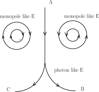
Figure 2: A sketch of the Y-like distribution of the color electric field obtained in lattice calculations in Ref. [7].

Our purpose here is to show that a similar distribution of force lines of the color electric field can be obtained in non-Abelian Yang-Mills-Proca theory with sources:

• Located at the vertices of the triangle $ABC$ and creating a Y-like profile of the gradient component of the color electric field:

  $$\vec{E}^{3,8}_{\text{grad}}=-\frac{1}{g}\nabla{h^{3,8}}.$$ (8)

  This component corresponds to the first term in the expression for the color electric field given by Eq. (5).

• Distributed along the sides of the triangle $ABC$ (see Fig. 1). These charge densities $\rho^{6,7}$ are needed for the creation of the components $A^{6,7}_{t}$ of the potential. According to the expression (5), the color electric field has two components: the gradient component $-\left(\gradient{h^{a}}\right)$, which is called the photon part in Ref. [7], and the nonlinear component $gf_{abc}A^{b}_{t}A^{c}_{i}$, which is called the monopole component in Ref. [7]. For $\vec{E}^{3,8}$, the nonlinear component is represented by the expression

  $$\vec{E}^{3,8}_{\text{nonlinear}}=\frac{\alpha}{2}\left(h^{6}\vec{A}^{7}-h^{7}\vec{A}^{6}\right),$$ (9)

  where $h^{6,7}=gA^{6,7}_{t}$; $\alpha=-1$ for $a=3$ and $\alpha=\sqrt{3}$ for $a=8$.

• Which are toroidal-like currents $\vec{j}\,^{6,7}$ (see Fig. 1) needed for the appearance of the color vector potentials $\vec{A}^{6,7}$ appearing in the expression (9).

The corresponding equations (18)-(23) describing a spatial distribution of the fields are given in Appendix A, since they are rather cumbersome.

III.2 Numerical method and boundary conditions

To solve numerically the set of sixteen partial differential equations (18)-(23), we rewrite them in terms of the dimensionless variables

$$\left(x,y,z\right)\to\frac{1}{m}\left(x,y,z\right),\quad\left(h^{a},v^{a},u^{a},w^{a}\right)\to m\left(h^{a},v^{a},u^{a},w^{a}\right),\quad j^{a\mu}\to\frac{m^{3}}{g}j^{a\mu}$$

and introduce compactified coordinates

$$\bar{x}=\frac{2}{\pi}\arctan\left(\frac{x}{c_{k}}\right),\bar{y}=\frac{2}{\pi}\arctan\left(\frac{z}{c_{k}}\right),\bar{z}=\frac{2}{\pi}\arctan\left(\frac{z}{c_{k}}\right),$$ (10)

which map the infinite region $(-\infty;\infty)$ onto the finite interval $[-1;1]$. Here $c_{k}$ is an arbitrary constant which is used to adjust the contraction of the grid. In our calculations, we typically take $c_{k}=4$.

Technically, Eqs. (18)-(23) are discretized on a grid consisting of $35\times 35\times 20$ grid points covering the integration region $-1\leq\bar{x},\bar{y}\leq 1$ and $0\leq\bar{z}\leq 1$ [given by the compactified coordinates (10)]. The resulting set of nonlinear algebraic equations is then solved by using a modified Newton method. The underlying linear system is solved with the Intel MKL PARDISO sparse direct solver [21] and the CESDSOL library.

Taking into account that the problem under consideration is symmetric with respect to the $z=0$ plane, one can conclude that profiles of the fields must be either symmetric or antisymmetric with respect to the $z=0$ plane. Then the boundary conditions can be taken in the form

$$\left.\partialderivative{h^{3,6,7,8}}{z}\right|_{z=0}= \left.\partialderivative{v^{6,7}}{z}\right|_{z=0}=\left.\partialderivative{u^{6,7}}{z}\right|_{z=0}=0,$$

$$\left.v^{3,8}\right|_{z=0}= \left.u^{3,8}\right|_{z=0}=\left.w^{3,6,7,8}\right|_{z=0}=0.$$

In turn, asymptotically (as $(x,y,z)\to\pm\infty$), all the above functions tend to 0. For such boundary conditions, the $\mathbb{Z}_{2}$ symmetry with respect to the $z=0$ plane results in the fact that the $z$-components of the electric and magnetic fields are $E^{3,6,7,8}_{z}(x,y,z=0)=H^{3,6,7}_{z}(x,y,z=0)=0$.

III.3 Numerical results and discussion

The numerical solutions of Eqs. (18)-(23) are shown in Figs. 3-6 for the following particular values of the system parameters appearing in the expressions (27)-(30): $l_{0}=5,d_{0}=4,\left(\rho_{0}\right)_{B}=\left(\rho_{0}\right)_{C}=-1/2\left(\rho_{0}\right)_{A}=-0.5,\rho_{1}=-0.2,x_{0}=3,y_{0}=-2,\alpha=2,\beta=4,j_{0}=-2,c=x_{0}$. The top left panel of Fig. 3 shows the Y-like distribution of force lines of the total electric field $\vec{E}^{3}$ which has two components: the gradient one given by Eq. (8) (the photon part in the terminology of Ref. [7]) and the nonlinear one given by Eq. (9) (the monopole part in the terminology of Ref. [7]).

The gradient components (8) for the electric fields $\vec{E}^{3,8}$ are shown in Fig. 3. They are sourced by the static quarks located at the vertices of the triangle $ABC$ with the color charge densities $\rho^{3,8}$ that are sources for the components $A^{3,8}_{t}$ of the non-Abelain potential $A^{3,8}_{\mu}$ in Eqs. (18) and (22).

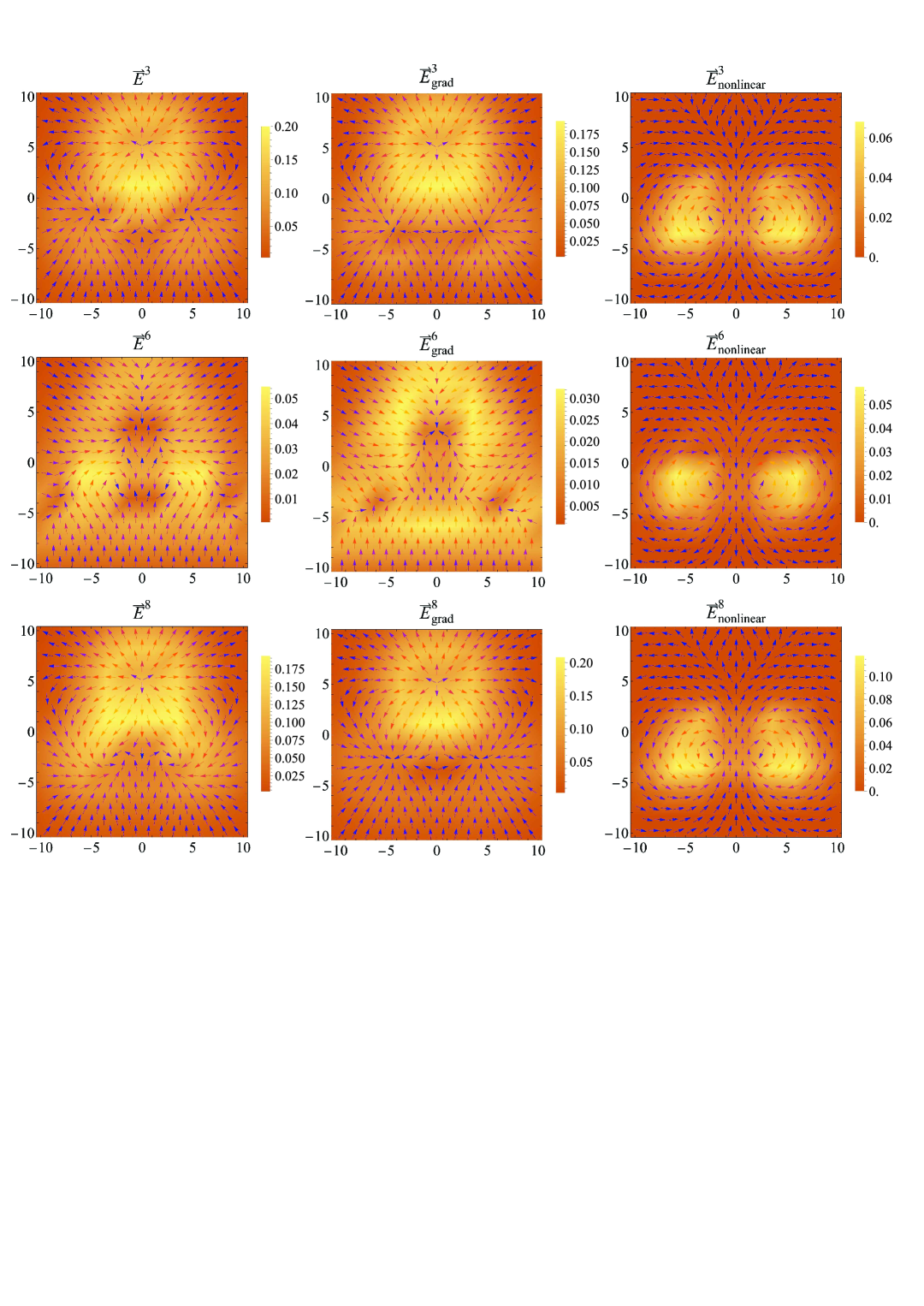
Figure 3: Force lines of the electric fields $\vec{E}^{3,6,8}$ in the $z=0$ plane.

The nonlinear components (9) for the electric fields $\vec{E}^{3,8}$ are shown in Fig. 3. According to Eq. (9), they are sourced by the components $A^{6,7}_{t}$ and $\vec{A}^{6,7}$ of the vector potential $A^{6,7}_{\mu}$.

The time components of the potentials $A^{3,6,8}_{t}=h^{3,6,8}$ are shown in Fig. 4. According to Eq. (5), the gradients of these components of the four-potential form the gradient components of the color electric fields $\vec{E}^{3,6,8}$.

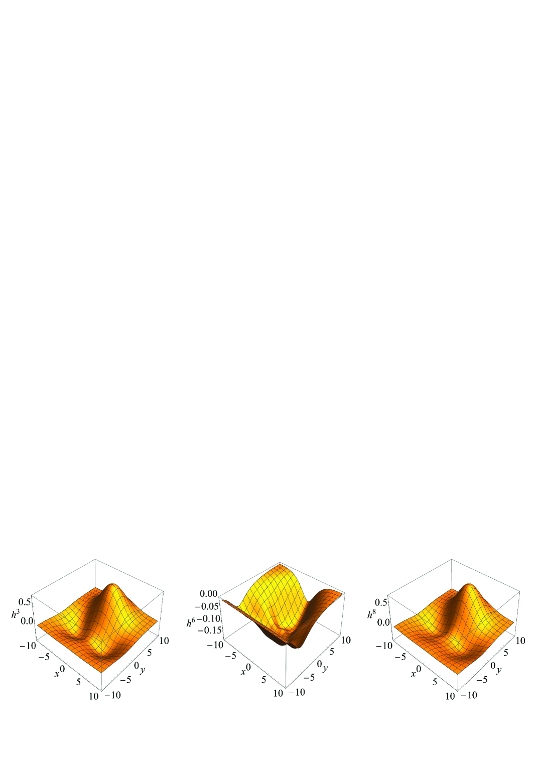
Figure 4: Potentials $A^{3,6,8}_{t}=h^{3,6,8}$ in the $z=0$ plane.

The components $\vec{A}^{6,7}$ that are needed to create the nonlinear components of the color electric fields are shown in Fig. 5, which also shows the spatial distribution of the potential $\vec{A}^{6}$. The results of numerical calculations indicate that $\vec{A}^{3,8}\approx 0$.

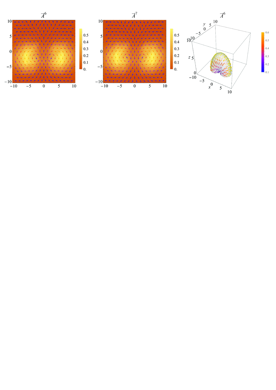
Figure 5: Force lines of the vector potentials $\vec{A}^{6,7}$ in the $z=0$ plane and the spatial distribution of the potential $\vec{A}^{6}$.

The color magnetic field $\vec{H}^{6}$ and its curl component are shown in Fig. 6, which also shows the spatial distribution of the magnetic field $\vec{H}^{6}$. The numerical calculations indicate that $\vec{H}^{3,8}\approx 0$. According to the numerical calculations, the spatial distribution of the magnetic field $\vec{H}^{7}$ is similar to that of $\vec{H}^{6}$.

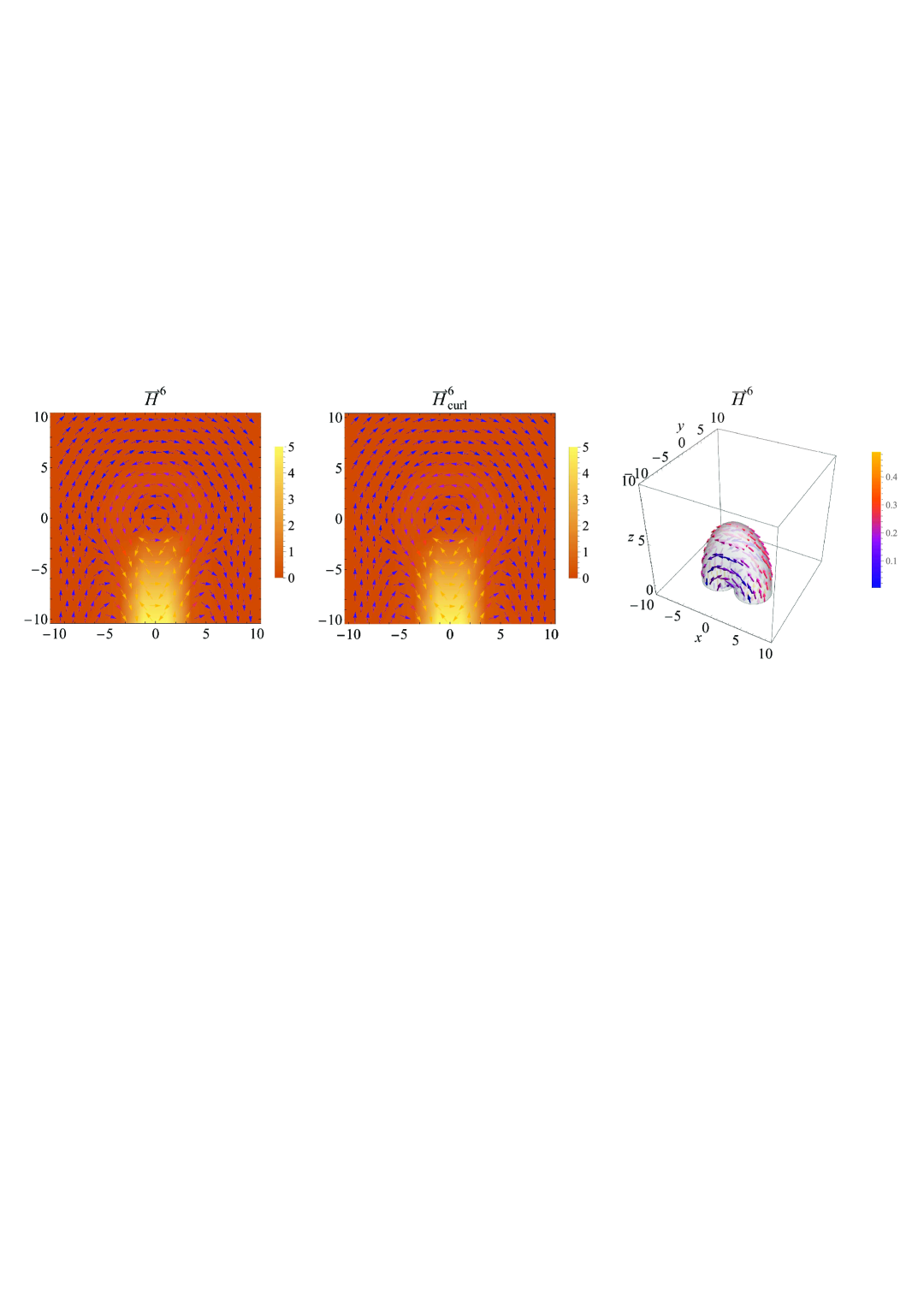
Figure 6: Force lines and the curl component of the color magnetic field $\vec{H}^{6}$ in the $y=0$ plane, as well as the spatial distribution of $\vec{H}^{6}$.

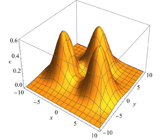
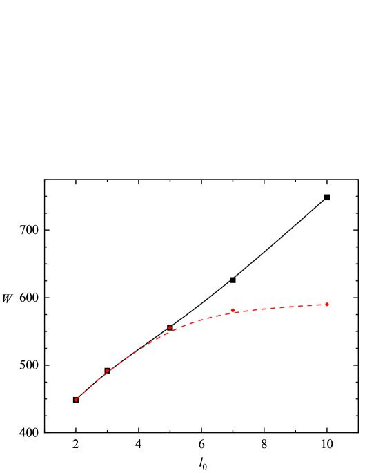
Figure 7: Left panel: the energy density $\varepsilon$ from Eq. (3) for the values of the system parameters given at the beginning of Sec. III.3. Right panel: the total energy $W$ from Eq. (12) as a function of $l_{0}$. The red dashed line is plotted for fixed geometric parameters $x_{0},y_{0},\alpha,\beta$, and the black solid line – for variable parameters.

Let us now turn to a comparison of the results obtained here with the results of Ref. [7] where the following static potential has been studied:

$$V^{3Q}\left(L_{Y}\right)=V^{3Q}_{0}-3\sqrt{3}\frac{\alpha^{3Q}}{L_{Y}}+\sigma^{3Q}L_{Y},$$ (11)

where $V^{3Q}_{0},\alpha^{3Q}$, and $\sigma^{3Q}$ are some parameters. $L_{Y}$ is a characteristic size in the given physical system; in our case it coincides in order of magnitude with $l_{0}$ (the length of the side of the triangle $ABC$). The second term on the right-hand side of the expression (11) describes the behavior of the static potential at small distances between quarks, and the third term corresponds to the confining potential. Note that the expression for $V^{3Q}$ contains monopole and photon parts, and the monopole term increases linearly for quite large $L_{Y}$, whereas the photon component remains approximately constant.

For comparison with those results, using the expression for the energy density from Eq. (3), we calculate the profile of the total energy of the configuration under consideration

$$W\left(l_{0}\right)=2\int_{0}^{\infty}\int_{-\infty}^{\infty}\int_{-\infty}^{\infty}\varepsilon(x,y,z)dxdydz$$ (12)

as a function of the characteristic size of our configuration $l_{0}$. The results of calculations are given in Fig. 7. The red dashed line is constructed for fixed geometric parameters describing our system: $l_{0}$ is a characteristic size of the system consisting of three quarks; $x_{0}$ and $y_{0}$ are the positions of the current densities $\vec{j}^{\,6,7}$; $\alpha$ and $\beta$ are parameters determining the profile of the current densities $\vec{j}\,^{6,7}$ (see Appendix B). It is seen that for rather large values of $l_{0}$ this profile differs considerably from a linear dependence predicted by lattice calculations. That is because when the characteristic distance between the static quarks increases, all the aforementioned parameters must also change, since actually (or in lattice calculations) a quantum system consisting of three quarks and of the fields created by them is self-consistent. Such self-consistency means that when the distance between the quarks changes, all other system parameters change as well. Consistent with this observation, for a quite large $l_{0}$, we choose the values of these parameters in such a way that we have a linear dependence (the black solid curve) of the total energy on the characteristic size $l_{0}$ between the quarks. In Table 1, we show the values of these parameters for different $l_{0}$.

$l_{0}$	$x_{0}$	$y_{0}$	$\alpha$	$\beta$
2	3	-2	2	4
3	3	-2	2	4
5	3	-2	2	4
7	3.1	-2	2	4
10	7	-4	8	4

Table 1: The parameters $x_{0},y_{0},\alpha$, and $\beta$ for different $l_{0}$ of the black solid curve in the right panel of Fig. 7.

Summarizing the results obtained,

1. According to the results shown in Fig. 3, the color electric fields $\vec{E}^{3,8}$ have two well-distinguishable components – the gradient and nonlinear ones. The first component $\vec{E}^{3,8}_{\text{grad}}$ is sourced by the color charges $\rho^{3,8}$ on the right-hand sides of Eqs. (18) and (22). These charges are located at the vertices of the triangle $ABC$, and their densities are given by the expressions (27). According to Eq. (9), the nonlinear term $\vec{E}^{3,8}_{\text{nonlinear}}$ is created by the scalar potentials $h^{6,7}$ and the vector potentials $\vec{A}^{6,7}$ (see also the item 5 below).

2. Comparison of the profiles of the color electric fields shown in Fig. 3 reveals a good agreement of our results with the results obtained in lattice calculations. In both cases, there are:

   1. the Y-like distribution for the total color electric fields $\vec{E}^{3,8}$, see the left panels in the top and bottom rows of Fig. 3;

   2. the Y-like distribution for the gradient component of the electric field (the photon-like component in terms of lattice calculations of Ref. [7]), compare the middle panels in the top and bottom rows of our Fig. 3 and Figure 9 of Ref. [7];

   3. the curl component of the electric field (the monopole-like component in terms of lattice calculations of Ref. [7]), compare the right panels in the top and bottom rows of our Fig. 3 and Figure 9 of Ref. [7].

3. Since the densities of the color charges $\rho^{3,8}$ have the same profile, the electric fields $\vec{E}^{3,8}$ have the same structure.

4. There are no sources for the potentials $h^{6,7}$ in Eq. (20), and therefore the electric field in the middle panel in the second row of Fig. 3 has no sources. This field is created by the nonlinear terms in Eq. (20).

5. The lattice calculations of Ref. [7] indicate that the color electric field has a monopole component sourced by a solenoidal current. In order to have such a component in our calculations, it is necessary to have solenoidal current densities $\vec{j}^{6,7}$ in Eq. (21); for this purpose, we use the expression (30) given in Appendix B.

6. The magnetic fields $\vec{H}^{6,7}$ have a toroidal structure when the force lines are basically concentrated inside the solenoid created by the currents $\vec{j}^{6,7}$, see the right panel of Fig. 6.

7. The magnetic fields $\vec{H}^{3,8}\approx 0$. This result has the explanation that, according to Eq. (6), these fields have two components: the curl one, $\vec{H}^{3,8}_{\text{curl}}=\curl{\vec{A}^{3,8}}$, and the nonlinear one, $\vec{H}^{3,8}_{\text{nonlinear}}\propto\left[\vec{A}^{6}\times\vec{A}^{7}\right]$; since $\vec{A}^{3,8}\approx 0$, and the vectors $\vec{A}^{6}$ and $\vec{A}^{7}$ are parallel, both these components are zero vectors.

8. The profile of the energy density shown in Fig. 7 (left panel) resembles (at least qualitatively) the profile of the Abelian action density shown in Figures 10 and 12 of Ref. [7].

9. We have obtained the profile of the total energy as a function of the characteristic size of the configuration under consideration. It is shown that this profile coincides qualitatively with the behavior of the photon component of the static potential obtained in lattice calculations of Ref. [7].

IV Discussion of the connection with lattice calculations

The results of calculations presented in Sec. III indicate that there is at least a qualitative agreement with the results of lattice calculations: (a) we have obtained the Y-like distribution of the color electric field with the sources in the form of static quarks located at the vertices of the triangle; (b) there is the Y-like component of the gradient color electric field; (c) there is the curl component of this field.

It enables us to assume that there may exist some connection between nonperturbative QCD, for which the results can be obtained in lattice calculations, and Yang-Mills-Proca theory under consideration. We assume that Yang-Mills-Proca theory may serve as some approximation to nonperturbative QCD as follows.

According to W. Heisenberg [17], the procedure of nonperturbative quantization consists in writing out quantum averages of the Yang-Mills and Dirac operator equations. But since these equations contain Green’s functions of different orders, to close the system, one has to write out equations for higher-order Green’s functions, and so on, ad infinitum. As a result, this leads to an infinite set of Dyson-Schwinger-type equations for all Green’s functions. Such approach is discussed in Ref. [18] for quantizing the $\phi^{4}$ field theory.

This approach is based on the operator Yang-Mills-Dirac field equations,

$$\hat{F}^{a\mu\nu}_{;\nu}= -\hat{j}^{a\mu}=-\hat{\bar{\psi}}\lambda^{a}\gamma^{\mu}\hat{\psi},$$ (13)

$$D_{\mu}\hat{\psi}-m\hat{\psi}= 0.$$ (14)

Since such operator equations cannot be solved analytically, they are solved by representing them as an infinite set of equations for the Green’s functions. In the first equation, which is derived by quantum averaging the equation (13), we have a differential equation for $\left\langle\hat{A}^{a}_{\mu}\right\rangle$. But in this case the resulting equation contains higher-order Green’s functions for which one has to write the corresponding equations, and so on, ad infinitum. The same is true for the operator Dirac equation (14). As a result, we will have an infinite set of equations for all Green’s functions. This process has been discussed in Refs. [19, 20]. In perturbative quantum theory these Dyson-Schwinger-type equations are solved using Feynman diagrams. In our case we have the following infinite set of equations:

$$\left\langle Q\right|\hat{F}^{a\mu\nu}\left|Q\right\rangle_{;\nu}= -\left\langle Q\right|\hat{j}^{a\mu}\left|Q\right\rangle,$$ (15)

$$\left\langle Q\right|\hat{A}_{\rho}\hat{F}^{a\mu\nu}\left|Q\right\rangle= -\left\langle Q\right|\hat{A}_{\rho}\hat{j}^{a\mu}\left|Q\right\rangle,$$ (16)

$$\ldots \,,$$ (17)

where $\left.\left.\right|Q\right\rangle$ is a quantum state describing the given physical situation. The first of these equations (15) contains the term that can schematically be represented in the form $\left\langle Q\right|\hat{A}^{a}_{\alpha}\hat{A}^{m}_{\beta}\hat{A}^{n}_{\gamma}\left|Q\right\rangle$, where $a=3,6,7,8$ and $A^{3,6,7,8}$ belong to the subgroup of SU(3), $m=1,2,4,5$. One can assume that $\left\langle Q\right|\hat{A}^{3,6,7,8}_{\mu}\left|Q\right\rangle\approx A^{3,6,7,8}_{\mu}$, whereas $\left\langle Q\right|\hat{A}^{m}_{\mu}\left|Q\right\rangle\approx 0$. Physically this means that, in some approximation in some processes in QCD, there are almost classical, $A^{3,6,7,8}_{\mu}$, and pure quantum, $A^{1,2,4,5}_{\mu}$, degrees of freedom. This enables one to assume that there is some quantum gluon condensate of purely quantum degrees of freedom, $\left\langle Q\right|\hat{A}^{m}_{\beta}\hat{A}^{n}_{\gamma}\left|Q\right\rangle\neq 0$, whose presence results in the appearance of the mass term $m^{2}$ in Eqs. (18)-(26).

In our calculations, the right-hand side of Eq. (15) is approximated by the color electric charge densities $\rho^{3,6,7,8}$ and by the color current densities $\vec{j}^{6,7}$. In a self-consistent problem, where the fields $A^{a}_{\mu}$ are sourced by quarks, the densities $\rho^{3,6,7,8}=\left\langle Q\right|\hat{\bar{\psi}}\gamma^{0}\lambda^{3,6,7,8}\hat{\psi}\left|Q\right\rangle$ and $\hat{\psi}$ is a spinor field describing quarks. One can suggest the following physical treatment of these densities: $\rho^{3,8}=\left\langle Q\right|\hat{\bar{\psi}}\gamma^{0}\lambda^{3,8}\hat{\psi}\left|Q\right\rangle\neq 0$ describes the fact that the quarks are located at the vertices $A,B,C$. Since the quarks are rotating, $\rho^{6,7}=\left\langle Q\right|\hat{\bar{\psi}}\gamma^{0}\lambda^{6,7}\hat{\psi}\left|Q\right\rangle\neq 0$ implies that there is nonzero probability to find quarks on the sides of the triangle $ABC$.

The physical interpretation of the currents $\left\langle Q\right|\hat{\vec{j}}^{6,7}\left|Q\right\rangle$ is not completely clear. One of options is that these currents may be created by quarks. Another possibility is that this can be nonzero quantum average of purely quantum degrees of freedom $\left\langle Q\right|\hat{A}^{m}_{\mu}\left|Q\right\rangle\approx 0$, whereas their bilinear combination remains nonzero: $f^{(6,7)mn}\left\langle Q\right|\hat{A}^{m}\hat{A}^{n}\left|Q\right\rangle\neq 0$.

Summarizing, we can say that, in lattice calculations, one is actually solving the field operator Yang-Mills-Dirac equations (13) and (14), whereas, in our calculations, we seek an approximate solution of these equations by solving only the equation (15) using some assumption concerning the form of the term $\left\langle Q\right|\hat{A}^{a}_{\alpha}\hat{A}^{m}_{\beta}\hat{A}^{n}_{\gamma}\left|Q\right\rangle$.

V Conclusions

Thus we have shown that, within SU(3) non-Abelian Yang-Mills-Proca theory with external sources, there are solutions that, at least qualitatively, agree with the results of lattice calculations in QCD: there is the Y-like distribution of the color electric field, as well as the curl component of this electric field. The Y-like distribution of the electric field is created by static quarks located at the vertices of an equilateral triangle.

Let us enumerate the main results of the study:

• We have obtained regular solutions within Yang-Mills-Proca theory with external sources in the form of: (a) color charges (simulating quarks) located at the vertices of the triangle; (b) charges distributed along the sides of this triangle; (c) solenoidal currents.

• It is shown that the color electric and magnetic fields have two components: the gradient/curl term for the electric/magnetic field, respectively, and the nonlinear component is present in both cases.

• It is shown that the distribution of the color electric field adequately represents the results obtained in lattice calculations: this field has a Y-like distribution, and the curl electric field is also present.

• The presence of the Y-like field is caused by the quarks located at the vertices of the triangle. The curl electric field is sourced by the solenoidal currents.

• The color magnetic field has only $\vec{H}^{6,7}$ nonzero components. The components $\vec{H}^{3,8}\approx 0$, since $\vec{A}^{3,8}\approx 0$ and the potentials $\vec{A}^{6,7}$ are parallel to each other.

• We have obtained the energy profile as a function of the characteristic distance between quarks for a system with variable geometric parameters; this profile coincides qualitatively with the profile of the photon part of the static potential obtained in Ref. [7].

• We suggest the model of possible connection between the results obtained here and the results obtained in lattice calculations, according to which, in lattice calculations, the field operator Yang-Mills-Dirac equations (13) and (14) are actually solved, whereas, in our calculations, an approximate solution of these equations is sought by solving only the equation (15) using some assumption about the form of the term $\left\langle Q\right|\hat{A}^{a}_{\alpha}\hat{A}^{m}_{\beta}\hat{A}^{n}_{\gamma}\left|Q\right\rangle$.

Note that a comparison of the results obtained in lattice calculations and the results obtained in the direction presented here may lead to a considerable improvement in understanding of the physical processes occurring in nonperturbative QCD.

Appendix A Equations for numerical calculations

For the potentials (4), the field equations (2) take the form

$$\laplacian{h^{3}}-m^{2}h^{3}-\frac{g}{2}\divergence{\left(h^{6}\vec{A}^{7}-h^{7}\vec{A}^{6}\right)}-\frac{g}{2}\left(-\vec{A}^{6}\cdot\vec{E}^{7}+\vec{A}^{7}\cdot\vec{E}^{6}\right)=\rho^{3},$$ (18)

$$\left(\curl{\curl{\vec{A}^{\,3}}}\right)_{i}+m^{2}A^{3}_{i}-\frac{g}{2}\partial_{j}\left(A^{6}_{i}A^{7}_{j}-A^{7}_{i}A^{6}_{j}\right)-\frac{g}{2}\left(h^{6}E^{7}_{i}-\left[\vec{A}^{\,6}\times\vec{H}^{7}\right]_{i}-h^{7}E^{6}_{i}+\left[\vec{A}^{\,7}\times\vec{H}^{6}\right]_{i}\right)=j^{3}_{i},$$ (19)

$$\laplacian{h^{6,7}}-m^{2}h^{6,7}+\frac{g}{2}\divergence{\left[\left(h^{3}-\sqrt{3}h^{8}\right)\vec{A}^{\,7,6}-h^{7,6}\left(\vec{A}^{\,3}-\sqrt{3}\vec{A}^{\,8}\right)\right]}$$

$$+\frac{g}{2}\left[\vec{A}^{\,7,6}\cdot\left(\vec{E}^{3}-\sqrt{3}\vec{E}^{8}\right)+\vec{E}^{7,6}\cdot\left(-\vec{A}^{\,3}+\sqrt{3}\vec{A}^{\,8}\right)\right]=\rho^{6,7},$$ (20)

$$\left(\curl{\curl{\vec{A}^{6,7}}}\right)_{i}+m^{2}A^{6,7}_{i}+\frac{g}{2}\partial_{j}\left[\left(A^{3}_{i}-\sqrt{3}A^{8}_{i}\right)A^{7,6}_{j}-A^{7,6}_{i}\left(A^{3}_{j}-\sqrt{3}A^{8}_{j}\right)\right]$$

$$+\frac{g}{2}\left\{\left(h^{3}-\sqrt{3}h^{8}\right)E^{7,6}_{i}-h^{7,6}\left(E^{8}_{i}-\sqrt{3}E^{3}_{i}\right)+\left[\vec{A}^{\,7,6}\times\left(\vec{H}^{3}-\sqrt{3}\vec{H}^{8}\right)\right]_{i}-\left[\left(\vec{A}^{\,3}-\sqrt{3}\vec{A}^{\,8}\right)\times\vec{H}^{7,6}\right]_{i}\right\}=j^{6,7}_{i},$$ (21)

$$\laplacian{h^{8}}-m^{2}h^{8}+\frac{g}{2}\divergence{\left[\vec{A}^{\,6}\left(h^{3}-\sqrt{3}h^{8}\right)-h^{6}\left(\vec{A}^{\,3}-\sqrt{3}\vec{A}^{\,8}\right)\right]}-\frac{\sqrt{3}}{2}g\left(\vec{A}^{\,6}\cdot\vec{E}^{7}-\vec{A}^{\,7}\cdot\vec{E}^{6}\right)=\rho^{8},$$ (22)

$$\left(\curl{\curl{\vec{A}^{\,8}}}\right)_{i}+m^{2}A^{8}_{i}+\frac{\sqrt{3}}{2}g\,\partial_{j}\left(A^{6}_{i}A^{7}_{j}-A^{7}_{i}A^{6}_{j}\right)+\frac{\sqrt{3}}{2}g\left(h^{6}E^{7}_{i}-h^{7}E^{6}_{i}-\left[\vec{A}^{\,6}\times\vec{H}^{7}\right]_{i}+\left[\vec{A}^{\,7}\times\vec{H}^{6}\right]_{i}\right)=j^{8}_{i},$$ (23)

where $\vec{A}^{a}=\left\{v^{a},u^{a},w^{a}\right\}$.

The components of Eq. (7) have the following explicit form (henceforth we consider the case where $j_{z}^{3,8}=0$ but $j_{z}^{6,7}\neq 0$):

$$m^{2}\divergence{\vec{A}^{\,3}}= \divergence{\vec{j}^{\,3}}-\frac{g}{2}\left(A^{7}_{t}\rho^{6}-\vec{A}^{\,7}\cdot\vec{j}^{\,6}-A^{6}_{t}\rho^{7}+\vec{A}^{\,6}\cdot\vec{j}^{\,7}\right),$$ (24)

$$m^{2}\divergence{\vec{A}^{\,6,7}}= \divergence{\vec{j}^{\,6,7}}\mp\frac{g}{2}\left[A^{3}_{t}\rho^{7,6}-\vec{A}^{\,3}\cdot\vec{j}^{\,7,6}-A^{7,6}_{t}\rho^{3}+\vec{A}^{\,7,6}\cdot\vec{j}^{\,3}\right.$$

$$\left.+\sqrt{3}\left(A^{7,6}_{t}\rho^{8}-\vec{A}^{\,7,6}\cdot\vec{j}^{\,8}-A^{8}_{t}\rho^{7,6}+\vec{A}^{\,8}\cdot\vec{j}^{\,7,6}\right)\right],$$ (25)

$$m^{2}\divergence{\vec{A}^{\,8}}= \divergence{\vec{j}^{\,8}}+\frac{\sqrt{3}}{2}g\left(A^{7}_{t}\rho^{6}-\vec{A}^{\,7}\cdot\vec{j}^{\,6}-A^{6}_{t}\rho^{7}+\vec{A}^{\,6}\cdot\vec{j}^{\,7}\right).$$ (26)

In Eq. (25), the choice of the sign “$-$” in front of the square brackets corresponds to the equation for the divergence of $\vec{A}^{\,6}$, and the choice of the sign “+” – to the equation for the divergence of $\vec{A}^{\,7}$. To get rid of mixed derivatives in Eqs. (19), (21), and (23), it is necessary to use the known relation $\curl{\curl{\vec{A}^{\,3,6,7,8}}}=\gradient{\left(\divergence{\vec{A}^{\,3,6,7,8}}\right)}-\laplacian{\vec{A}^{\,3,6,7,8}}$, as well as the relations (24)-(26). After such substitution, all the equations (18)-(23) are of the elliptic type, and they can be numerically solved using the CESDSOL library. It is worth pointing out, however, that after such procedure the resulting equations contain derivatives of the sources, $\partial_{\mu}j^{b}_{\nu}$.

Appendix B Densities of color charges and currents

The charge densities $\rho^{3,8}_{A,B,C}$ of static quarks located at the vertices of the triangle $ABC$ (see Fig. 1) are

$$\rho^{3,8}_{A,B,C}=\left(\rho_{0}\right)_{A,B,C}\exp{-\frac{\left(x-x_{A,B,C}\right)^{2}}{d_{0}^{2}}-\frac{\left(y-y_{A,B,C}\right)^{2}}{d_{0}^{2}}-\frac{\left(z-z_{A,B,C}\right)^{2}}{d_{0}^{2}}}.$$ (27)

Here $\left(\rho_{0}\right)_{A,B,C}$ are three parameters describing the magnitude of charges located at the vertices of the triangle $ABC$: $\left(\rho_{0}\right)_{B}=\left(\rho_{0}\right)_{C}=-1/2\left(\rho_{0}\right)_{A}$; $d_{0}$ is a characteristic size of the distribution of these charges; $(x,y,z)_{A,B,C}$ are $x,y,z$-coordinates of the vertices $A,B,C$. These charge densities serve as sources in Eqs. (18) and (22):

$$\rho^{3,8}=\rho^{3,8}_{A}+\rho^{3,8}_{B}+\rho^{3,8}_{C}.$$ (28)

Analytical expressions for the densities $\rho^{6,7}$ are

$$\rho^{6,7}= \rho_{AB}+\rho_{BC}+\rho_{CA}=\frac{\rho_{1}}{4}\left[\tanh(x)+1\right]\left[\tanh\left(\frac{x}{\sqrt{3}}+y\right)+1\right]$$

$$\exp\left\{-\frac{\left(x-\frac{-b_{AB}k_{AB}+k_{AB}y+x}{k_{AB}^{2}+1}\right)^{2}+\left[-\frac{k_{AB}\left(-b_{AB}k_{AB}+k_{AB}y+x\right)}{k_{AB}^{2}+1}-b_{AB}+y\right]^{2}+z^{2}}{d_{0}^{2}}\right\}+$$

$$\frac{\rho_{1}}{4}\left[\tanh\left(\frac{x}{\sqrt{3}}-y\right)+1\right]\left[1-\tanh\left(\frac{x}{\sqrt{3}}+y\right)\right]\exp{-\frac{\left(y-b_{\text{BC}}\right)^{2}+z^{2}}{d_{0}^{2}}}+$$

$$\frac{\rho_{1}}{4}\left[1-\tanh(x)\right]\left[1-\tanh\left(\frac{x}{\sqrt{3}}-y\right)\right]$$

$$\exp{-\frac{\left(x-\frac{-b_{AC}k_{AC}+k_{AC}y+x}{k_{AC}^{2}+1}\right)^{2}+\left[-\frac{k_{AC}\left(-b_{AC}k_{AC}+k_{AC}y+x\right)}{k_{AC}^{2}+1}-b_{AC}+y\right]^{2}+z^{2}}{d_{0}^{2}}}.$$ (29)

Here $\rho_{AB}$ is the density of a color electric charge located on the side $AB$ of the triangle $ABC$ (similarly, for $\rho_{BC}$ and $\rho_{CA}$). The equation $-b_{AB}k_{AB}+k_{AB}y+x=0$ is an equation of a straight line perpendicular to the side $AB$ which passes through the vertex $A$. An equation of a straight line passing through the points $A$ and $B$ (the side $AB$) is $y=k_{AB}x+b_{AB}$. An equation for a straight line perpendicular to the side $AB$ which passes through the vertex $B$ is written similarly. An equation for a straight line for the side $BC$ is $y=b_{BC}$. The factor with the exponent is chosen so that the charge density decreases exponentially in the direction perpendicular to the side $AB$. The factors $\left[\tanh(x)+1\right]$ and $\left[\tanh\left(\frac{x}{\sqrt{3}}+y\right)+1\right]$ are chosen so as to approximate a step function restricting $\rho_{AB}$ by the straight lines passing through the vertices $A$ and $B$ (similarly, for $\rho_{BC}$ and $\rho_{CA}$). For better understanding of the distributions of the densities (28) and (29), Fig. 8 shows the profiles of $\rho^{3,8}$ and $\rho^{6,7}$.

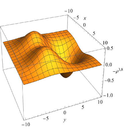
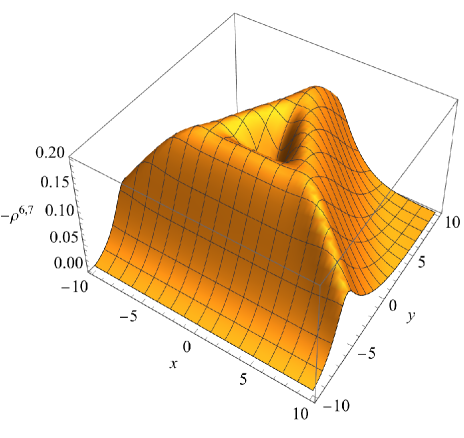
Figure 8: The profiles of the color electric charge densities $\rho^{3}=\rho^{8}$ and $\rho^{6}=\rho^{7}$ in the $z=0$ plane.

For the solenoidal current densities $\vec{j}^{\,6,7}$, we employ some functions that are needed on transforming to toroidal coordinates. The necessary details about toroidal coordinates $\left(\tau,\sigma,\varphi\right)$ are given in Appendix C. Using the vector (35) tangent to the torus, we introduce the solenoidal current density $\vec{j}^{\,7}=-\vec{j}^{\,6}$ as follows:

$$\vec{j}^{\,6}=j_{0}\vec{h}^{\varphi}\left[-\frac{\beta}{\bar{\tau}}+\frac{\beta}{\bar{\tau}\left(x_{0},y_{0},0\right)}\right]\exp\left[-\frac{\beta}{\bar{\tau}}+\frac{\beta}{\bar{\tau}\left(x_{0},y_{0},0\right)}\right],$$ (30)

where $\bar{\tau}=\left[1-e^{-2\tau\left(x,y-y_{0},z\right)}\right]^{\alpha}$, $x_{0}=c$, and the function $\tau(x,y,z)$ is given by the expression (31). The parameters $x_{0}$ and $y_{0}$ specify the location of the circle $x^{2}+z^{2}=x_{0}^{2}$ in the $y=y_{0}$ plane; $j_{0}$ is a parameter specifying the magnitude of the current density, and $\alpha$ and $\beta$ are some parameters controlling the profile of the solenoidal current. The profile of this current on a torus with some $\tau=\text{const}$ is exemplified by Fig. 9.

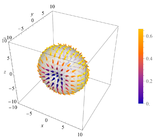
Figure 9: The profile of the current $\vec{j}^{\,6}$ given by Eq. (30).

Appendix C Toroidal coordinates

The transformation from toroidal coordinates $(\tau,\sigma,\varphi)$ to Cartesian coordinates $(x,y,z)$ is performed using the formulas

$$\tau= \log\left(\sqrt{\frac{\left(\sqrt{x^{2}+z^{2}}+c\right)^{2}+y^{2}}{\left(\sqrt{x^{2}+z^{2}}-c\right)^{2}+y^{2}}}\right),$$ (31)

$$\sigma= \arccos\left(\frac{-c^{2}+x^{2}+y^{2}+z^{2}}{\sqrt{\left(-c^{2}+x^{2}+y^{2}+z^{2}\right)^{2}+4c^{2}y^{2}}}\right),$$ (32)

$$\varphi= \arctan\left(\frac{z}{x}\right),$$ (33)

where the parameter $c$ specifies the location of the circle $x^{2}+z^{2}=c^{2},y=0$. The expression $\tau=\text{const}$ specifies the equation of a torus.

The square of the linear element is given by the expression

$$dl^{2}=\frac{c^{2}}{\left(\cosh\tau-\cos\sigma\right)^{2}}\left(d\tau^{2}+d\sigma^{2}+\sinh^{2}\tau d\varphi^{2}\right)=h^{a}_{\phantom{a}i}h_{aj}dx^{i}dx^{j},$$

where $i,j$ are spatial indices and $a$ is a triad index. The triad

$$h^{a}_{\phantom{a}i}=\frac{1}{\cosh\tau-\cos\sigma}\begin{pmatrix}\partial_{x}\tau&\partial_{y}\tau&\partial_{z}\tau\\ \partial_{x}\sigma&\partial_{y}\sigma&\partial_{z}\sigma\\ \sinh\tau\partial_{x}\varphi&\sinh\tau\partial_{y}\varphi&\sinh\tau\partial_{z}\varphi\end{pmatrix}.$$ (34)

The unit vector

$$h^{3}_{\phantom{3}i}=h^{\varphi}_{\phantom{\varphi}i}=N\left\{-4x\left(y-y_{0}\right),2\left(x^{2}-x_{0}^{2}-\left(y-y_{0}\right)^{2}+z^{2}\right),-4z\left(y-y_{0}\right)\right\}$$ (35)

is tangent to a torus in the $\varphi=\text{const}$ plane, and

$$N=\left\{\left[2\left(x^{2}-x_{0}^{2}-(y-y_{0})^{2}+z^{2}\right)\right]^{2}+16x^{2}\left(y-y_{0}\right)^{2}+16z^{2}\left(y-y_{0}\right)^{2}\right\}^{-1/2}$$

is the factor normalizing the vector (34) to unity.

References

- [1] M. Constantinou, A. Courtoy, M. A. Ebert, M. Engelhardt, T. Giani, T. Hobbs, T. J. Hou, A. Kusina, K. Kutak, and J. Liang, et al. Prog. Part. Nucl. Phys. 121, 103908 (2021).
- [2] K. Cichy and M. Constantinou, Adv. High Energy Phys. 2019, 3036904 (2019).
- [3] H. T. Ding, F. Karsch, and S. Mukherjee, Int. J. Mod. Phys. E 24, 1530007 (2015).
- [4] C. Alexandrou, M. Constantinou, K. Hadjiyiannakou, K. Jansen, C. Kallidonis, G. Koutsou, A. Vaquero Avilés-Casco, and C. Wiese, Phys. Rev. Lett. 119, 142002 (2017).
- [5] A. Di Giacomo, M. Maggiore, and S. Olejnik, Nucl. Phys. B 347, 441 (1990).
- [6] G. S. Bali, K. Schilling, and C. Schlichter, Phys. Rev. D 51, 5165 (1995).
- [7] V. G. Bornyakov et al. [DIK], Phys. Rev. D 70, 054506 (2004).
- [8] Y. Koma and M. Koma, Phys. Rev. D 95, 094513 (2017).
- [9] N. Sakumichi and H. Suganuma, Phys. Rev. D 92, 034511 (2015).
- [10] C. A. R. Herdeiro, A. M. Pombo, and E. Radu, Phys. Lett. B 773, 654 (2017).
- [11] V. Dzhunushaliev and V. Folomeev, Phys. Rev. D 99, 104066 (2019).
- [12] V. Dzhunushaliev and V. Folomeev, Phys. Rev. D 101, 024023 (2020).
- [13] V. Dzhunushaliev and V. Folomeev, Phys. Rev. D 104, 104024 (2021).
- [14] A. De Felice, L. Heisenberg, R. Kase, S. Mukohyama, S. Tsujikawa, and Y. l. Zhang, JCAP 06, 048 (2016).
- [15] S. Nakamura, R. Kase, and S. Tsujikawa, Phys. Rev. D 95, 104001 (2017).
- [16] M. Minamitsuji, Phys. Rev. D 94, 084039 (2016).
- [17] W. Heisenberg, Introduction to the unified field theory of elementary particles (Max-Planck-Institut für Physik und Astrophysik, Interscience Publishers London, New York, Sydney, 1966).
- [18] C. M. Bender, K. A. Milton, and V. Savage, Phys. Rev. D 62, 085001 (2000).
- [19] M. Frasca, Eur. Phys. J. C 80, 707 (2020).
- [20] V. Dzhunushaliev and V. Folomeev, Found. Phys. 52, 118 (2022).
-
[21]
N.I.M. Gould, J.A. Scott, Y. Hu,
ACM Trans. Math. Softw. 33, 10 (2007);
O. Schenk, K. Gartner, Future Gener. Comput. Syst. 20, 475 (2004). - [22] C. Herdeiro, I. Perapechka, E. Radu, and Y. Shnir, Phys. Lett. B 797, 134845 (2019).
- [23] C. Herdeiro, I. Perapechka, E. Radu, and Y. Shnir, Phys. Lett. B 824, 136811 (2022).