Spacetime Grand Unified Theory

Abstract

The Standard Model of particle physics is derived from first principles starting from the free Dirac Lagrangian. All known fermionic particle species plus three right handed neutrinos are obtained from ideals of a $\mathcal{C}\ell_{8,0}$ algebra, with gauge symmetries arising as rotations of creation-annihilation operators and vacua. Triality originates both the strong force and three particle families with a mass hierarchy. Lorentz and gauge transformations are unified while avoiding the Coleman-Mandula theorem. Chirality stems unavoidably from rotations leaving the vacua invariant, with a predicted Weinberg angle of $\sin^{2}(\theta_{W})=3/8$. The theory is anomaly-free and devoid of proton decay.

I Introduction

Among the unexplained features of the Standard Model (SM), the chiral nature of the weak interaction, the choice of particle representations and the existence of three particle families stand out as particularly vexing. Grand Unified Theories (GUTs) arose as an attempt to explain some of these open problems while unifying the different gauge groups of the fundamental forces into a single one. The most famous GUTs, based on the groups $SU(5)$ Georgi:1974a , $SO(10)$ Georgi:1974b and $SU(4)_{C}\times SU(2)_{R}\times SU(2)_{L}$ Pati:1974 , offered some exciting possible solutions to some of the issues but carried with them the burden of proton decay whose experimental lifetime lower limit has ruled out most of them Ohlsson:2023 . Supersymmetry (SUSY) emerged as a promising framework for Grand Unified Theories (GUTs) Golfand:1971 ; Volkov:1972 ; Volkov:1973 ; Wess:1974a ; Wess:1974b , proposing a bosonic (fermionic) superpartner for each fermionic (bosonic) particle. This elegant symmetry resolves the hierarchy problem—arising from the unnatural smallness of the Higgs mass relative to the Planck scale—and offers a dark matter candidate in the lightest neutralino (c.f. for example Mohapatra:2003 for a complete overview on GUTs and SUSY). However, the Large Hadron Collider (LHC) has found no evidence of SUSY particles, which were expected to manifest within the current accessible energy ranges. Theoretically, additional assumptions can circumvent these experimental constraints, but they introduce new free parameters and undermine the naturalness that initially motivated SUSY’s appeal.

An algebraic alternative to GUTs and SUSY has been simultaneously developed over the decades, though it has received far less attention in comparison. This line of thought, typically centered on division algebras Gunaydin:1973a ; Gunaydin:1973b ; Dixon:1994 ; Leo:1996 ; Carrion:2003 ; Baez:2012 ; Baez:2011a ; Baez:2011b ; Huerta:2011 ; Huerta:2014 ; Furey:2015 ; Burdik:2017 ; Furey:2021 ; Furey:2022a ; Singh:2023 ; Furey:2022b ; Singh:2025 ; Furey:2016 ; Stoica:2018 ; Furey:2018b ; Todorov:2023 ; Lasenby:2023 ; Gording:2020 ; Manogue:2010 ; Boyle:2014 ; Boyle:2020 ; Bhatt:2022 ; Furey:2014 ; Furey:2025a ; Furey:2025b ; Todorov:2017 ; Furey:2018a ; Gillard:2019a ; Gillard:2019b or Clifford algebras Barducci:1977 ; Casalbuoni:1979a ; Casalbuoni:1979b ; Hestenes:1982 ; Cho:1995 ; Chisholm:1996 ; Lewis:1998 ; Trayling:2001 ; Trayling:2004 ; Doran:2003 ; Pavsic:2017 ; Stoica:2020 ; Borstnik:2023 ; Zenczykowski:2015 (c.f. references therein for a more complete list), has yielded intriguing insights. In particular, it demonstrates that the invariant symmetries of certain structures can give rise to symmetries related to the Standard Model (SM). For example, it is known that the algebras $\mathcal{C}\ell(7)$ and $\mathcal{C}\ell(8)$ have enough space to accommodate one and three copies, respectively, of the particle representations of the SM Chisholm:1996 ; Trayling:2004 ; Pavsic:2017 ; Gillard:2019b ; Furey:2021 . This approach, however, is limited by the ad hoc nature of the very structures involved, often leading to either an incomplete particle content or a surplus of unobserved particles, as well as a lack of testable predictions. Additional works have also focused on the problem of particle families by searching for possible connections with triality Silagadze:1995 ; YuFen:2006 ; Manogue:2010 ; Boyle:2014 ; Furey:2014 ; Todorov:2017 ; Furey:2018a ; Gillard:2019a ; Gillard:2019b ; Gording:2020 ; Boyle:2020 ; Bhatt:2022 ; Furey:2025a ; Furey:2025b , although no definite connection has been confirmed yet, partially due to the a priori non-unique reasoning for considering the phenomenon, as well as the lack of a predicted mass hierarchy. Consequently, the predictive power of these algebraic theories is still only comparable, at best, to that of standard GUTs. Furthermore, they typically overlook the quantization aspect (notable exceptions are Cho:1995 ; Zenczykowski:2015 ; Pavsic:2017 ).

In this work, we depart from the historical top-bottom approach of finding mathematical frameworks that can fit the SM gauge symmetries to a strict bottom-up first-principles approach. In particular, we show that the entire SM can be obtained starting from the free Dirac quantum field theory (QFT). This is achieved by first proving that a fermionic quantum field can be constructed using solely Witt basis vectors of a $\mathcal{C}\ell_{8,0}$ Clifford algebra, naturally representing creation-annihilation operators acting on minimal ideals. An embedding for the Dirac theory in 8-dimensional space is then obtained, unifying spinors and creation operators. The phenomenon of triality, characteristic of $\mathcal{C}\ell_{8,0}$, gives rise to two more distinct Dirac spinors representations, leading to a generalized Dirac equation with a mass matrix containing 3 families of particles per species. The minimal ideals, from which the QFT vacuum is constructed, inherit natural substructures from spinors in $\mathcal{C}\ell_{8,0}$, whose rotations have no physical consequences for the Lagrangian. This latter invariance is uniquely described by the SM group with unified gauge couplings, leading to all known particle representations plus three right handed neutrinos. The algebra of spacetime (i.e. the Dirac algebra) becomes unified in this way with the same algebra as gauge transformations, with particle multiplets related by reflections in spacetime. Ideals and Lie algebras become more than just entities associated to abstract groups, being directly connected to rotations of the quantum field vacuum which now transforms as (not just under) Clifford algebras, all the while avoiding proton decay. We call this unifying framework Spacetime Grand Unified Theory (SGUT).

II Quantum Fields as Clifford Algebra Elements

We begin by considering a free fermionic quantum field $\hat{\psi}(x)$ with mass $m$, living in a Minkowski spacetime with metric $\eta=\textrm{diag}(+1,-1,-,1,-1)$ and parametrized by the coordinates $x^{\mu}$. Such a theory is governed by the Lagrangian operator

$$\hat{\mathcal{L}}(x)=\hat{\psi}^{\dagger}_{\alpha}(x)(i(\gamma^{0}\gamma^{\mu})_{\alpha\beta}\partial_{\mu}-m(\gamma^{0})_{\alpha\beta})\hat{\psi}_{\beta}(x)$$ (1)

where $\gamma^{\mu}$ are the Dirac gamma matrices. We also assume the usual Einstein notation as well as the hat notation for infinite dimensional quantum operators. The gamma matrices obey the commutation relations

$$\{\gamma^{\mu},\gamma^{\nu}\}=2\eta^{\mu\nu}1_{4\times 4}$$ (2)

with $1_{n\times n}$ denoting the n-dimensional identity matrix, and so they generate the Clifford algebra $\mathcal{C}\ell_{1,3}$. Since $\gamma^{\mu}$ transform as 4-vectors with an inner product defined in Eq. (2), we will frequently call $\gamma^{\mu}$ by spacetime basis vectors as well, as they do span a basis for 4-vectors in spacetime. We will adopt the notation $\mathcal{C}\ell_{r,q}$ to denote a Clifford algebra generated by $r$ elements with norm $+1$ and $q$ elements with norm $-1$, or simply $\mathcal{C}\ell(n)$ for an non-specified $n$ dimensional metric. The quantum field $\hat{\psi}(x)$ can be expanded in the standard way Bjorken:1964 as ${\hat{\psi}_{\alpha}(x)=\int d\Pi\sum^{2}_{s=1}\bigg{(}\hat{a}^{s}_{\textbf{p}}u^{s}_{\alpha}(p)e^{-ip\cdot x}+\hat{b}^{s\dagger}_{\textbf{p}}v^{s}_{\alpha}(p)e^{ip\cdot x}\bigg{)}}$ where $d\Pi=\frac{d^{3}\textbf{p}}{(2\pi)^{3}}\frac{1}{\sqrt{2E_{\textbf{p}}}}$ is the invariant phase space volume element, $p$ is the 4-momentum vector, p is its spatial part and $E_{\textbf{p}}=\sqrt{m^{2}+|\textbf{p}|^{2}}$ is the energy. The spinors $u$ and $v$ are the solutions of the free Dirac equation, each with four components indexed by $\alpha$, and $\hat{a}^{s}_{\textbf{p}}$ and $\hat{b}^{s}_{\textbf{p}}$ are the creation operators obeying the commutation relations

$$\{\hat{a}^{s}_{\textbf{p}},\hat{a}^{r\dagger}_{\textbf{k}}\}=\{\hat{b}^{s}_{\textbf{p}},\hat{b}^{r\dagger}_{\textbf{k}}\}=(2\pi)^{3}\delta^{sr}\delta^{(3)}(\textbf{p}-\textbf{k})\,,$$ (3)

$$\{\hat{a}^{s}_{\textbf{p}},\hat{a}^{r}_{\textbf{k}}\}=\{\hat{a}^{s\dagger}_{\textbf{p}},\hat{a}^{r\dagger}_{\textbf{k}}\}=\{\hat{b}^{s}_{\textbf{p}},\hat{b}^{r}_{\textbf{k}}\}=\{\hat{b}^{s\dagger}_{\textbf{p}},\hat{b}^{r\dagger}_{\textbf{k}}\}=0\,.$$ (4)

It has been recognized Borstnik:2023 that the commutation relations Eqs. (3)-(4) are reminiscent of a Witt basis of an 8-dimensional Clifford algebra

$$\{\omega^{a},\omega^{b\dagger}\}=\delta^{ab}\,,\quad\{\omega^{a},\omega^{b}\}=\{\omega^{a\dagger},\omega^{b\dagger}\}=0\,,$$ (5)

constructed from a basis $\{e_{A}\}_{A=1,\ldots,8}$ of $\mathcal{C}\ell_{8,0}$ (i.e. such that $\{e_{A},e_{B}\}=2\delta_{AB}$, akin to Eq. (2)) via Lounesto:2001

$$\omega^{s}=\frac{ie_{s}+e_{9-s}}{2}\,,\quad s=1,\cdots,4\,.$$ (6)

However, one can actually construct fermionic creation and annihilation operators as infinite tensor products of $\mathcal{C}\ell_{8,0}$ algebras via Bott periodicity, such that $\hat{\psi}_{\alpha}(x)\in\mathcal{C}\ell_{8,0}\otimes\lim_{N\to\infty}(\mathcal{C}\ell_{8N,0})^{\otimes 3}$ (c.f. Sec. I of the Appendix). Consequently, just as relativistic invariance of quantum dynamics requires the introduction of the Clifford algebra $\mathcal{C}\ell_{1,3}$ and the Dirac equation, the quantization of its four independent solutions requires the introduction of the algebra $\mathcal{C}\ell_{8,0}$. We note that in Furey:2021 it is observed that Bott periodicity might be related to the construction of multiparticle states and possibly Fock spaces. This is then used as motivation to study $\mathcal{C}\ell_{0,8}$ as previous works using the same algebra Gillard:2019a ; Gillard:2019b (modulus metric signatures), i.e. by searching for structures whose invariant symmetries might lead to the SM, thus sharing the same setbacks as the remaining state-of-the-art. This latter approach shares no similarities with the one developed in this work, other than the focus on a $\mathcal{C}\ell(8)$ algebra (or Clifford algebras in general) as the setting to develop a theory of fundamental forces. In particular, the use of $\mathcal{C}\ell_{8,0}$ here is not postulated, emerging as a necessary consequence of second quantization, as shown by the novel proofs in Sec. I of the Appendix (which happen to use the Bott periodicity theorem). The works most closely aligned to this approach are Zenczykowski:2015 , where (first) quantization is connected to $\mathcal{C}\ell_{6,0}$ and Cho:1995 ; Pavsic:2017 , which considered explicit representations of fermionic quantum fields, living in the algebras $\mathcal{C}\ell_{1,3}\otimes\mathcal{C}\ell_{\infty}$ and $\mathcal{C}\ell_{8,0}\otimes\mathcal{C}\ell_{\infty}$, respectively. The proposal that the SM symmetries and particle representations might be embedded in $\mathcal{C}\ell(8)$ goes at least as far back as 2010, in the concluding remarks of Pavsic:2010 .

III Relativistic Quantum Mechanics in $\mathcal{C}\ell_{8,0}$

Having singled out the importance of $\mathcal{C}\ell_{8,0}$, one might explore whether it plays some other role in the theory described by the Lagrangian in Eq. (1). Note that the latter can be equivalently written as $\hat{\mathcal{L}}(x)=\hat{\psi}^{\dagger}_{\alpha}(x)X_{\alpha\beta}\hat{\psi}_{\beta}(x)$ where $X_{\alpha\beta}$ are the components of a $4\times 4$ matrix $X\in\mathcal{C}\ell_{1,3}$. Since the Dirac algebra is a subalgebra of $\mathcal{C}\ell_{8,0}$, it is natural to search for $X\in\mathcal{C}\ell_{8,0}$, i.e. for an embedding of the Dirac algebra in $\mathcal{C}\ell_{8,0}$. The latter question is equivalent to finding a set of four 16-dimensional matrices $\Gamma^{\mu}_{(+)}$ and a 16-dimensional diagonal matrix $P_{(+)}$ with only four non-zero elements equal to 1, such that

$$\{\Gamma^{\mu}_{(+)},\Gamma^{\nu}_{(+)}\}=2\eta^{\mu\nu}P_{(+)}\,,$$ (7)

where the subscript $(+)$ is adopted for future convenience. To find a natural representation, consider the four annihilation operators of a single momentum mode

$$a^{1}_{\textbf{p}}=\omega^{1},a^{2}_{\textbf{p}}=\omega^{2},b^{1}_{\textbf{p}}=\omega^{3},b^{2}_{\textbf{p}}=\omega^{4}\in\mathcal{C}\ell_{8,0}$$ (8)

in a lattice, where we focus solely on the Clifford algebra related to the spinorial quantization degrees of freedom (c.f. Sec. I of the Appendix). Defining the 16-dimensional matrix $V_{i}$ as

$$\left(V_{i}\right)_{ab}=\left\{\begin{array}[]{ll}1,&a=1,b=i\\ 0,&\textrm{otherwise.}\\ \end{array}\right.\,,\,\,\,\,(a,b=1,\ldots,16)$$ (9)

we find that $a^{s}_{\textbf{p}}V_{i}=b^{s}_{\textbf{p}}V_{i}=0\,,a^{s\dagger}_{\textbf{p}}V_{i}\neq 0\,,b^{s\dagger}_{\textbf{p}}V_{i}\neq 0$ for the explicit representation in Eq. (A37). In other words, $V_{i}$ satisfies the properties of a vacuum for any $i$, with the full quantum vacuum $\ket{0}$ constructed as a function of $V_{i}$ (c.f. Sec. I of the Appendix). A vital fact about $V_{i}$ is that, for any $X\in\mathcal{C}\ell_{8,0}$, $XV_{i}$ will result in a non-zero column $i$ and 0 everywhere else. The $V_{i}$ are thus minimal left ideals generating mutually independent spaces when multiplication is restricted to the left. Contact with spinors is then obtained by considering them to be matrices of the form $XV_{i}$ instead of the standard one-column representation. In particular, rest frame spinors in the Dirac representation are given by 1-column constant vectors with a single non-zero entry equal to 1 Bjorken:1964 but could just as well be taken as 4-dimensional matrices with a single non-zero element. The latter fact establishes a picture in $\mathcal{C}\ell_{8,0}$ by noting that, for example, $a^{1\dagger}_{\textbf{p}=0}V_{i}$ not only physically corresponds to the creation of a mode associated to the spinor $u^{1}(0)$ but also, due to the representation (8), is only non-zero in column $i$ with a single non-zero entry equal to 1. This immediately leads to the natural identification of rest spinors as 16-dimensional matrices

$$u^{1}_{16D}(\textbf{p}=0) =a^{1\dagger}_{\textbf{p}=0}V_{i}=\omega^{1\dagger}V_{i}\,,$$ (10)

$$u^{2}_{16D}(\textbf{p}=0) =a^{2\dagger}_{\textbf{p}=0}V_{i}=\omega^{2\dagger}V_{i}\,,$$ (11)

$$v^{1}_{16D}(\textbf{p}=0) =b^{1\dagger}_{\textbf{p}=0}V_{i}=\omega^{3\dagger}V_{i}\,,$$ (12)

$$v^{2}_{16D}(\textbf{p}=0) =b^{2\dagger}_{\textbf{p}=0}V_{i}=\omega^{4\dagger}V_{i}\,.$$ (13)

It bears emphasizing that while the connection between the Witt basis of $\mathcal{C}\ell_{8,0}$ and creation-annihilation operators has been noted in the literature (c.f. Borstnik:2023 and references therein), the unification of the algebra of the creation operators for a single momentum mode with that of the spinors they create has never been realized. Notably, this result would be impossible to attain in $\mathcal{C}\ell_{1,3}$, since its Witt basis possesses only two independent vectors. The algebra of $\mathcal{C}\ell_{8,0}$ is thus the simplest one where creation operators for a single momentum mode and Dirac spinors can be unified, reinforcing the importance of $\mathcal{C}\ell_{8,0}$. We can now obtain a representation for $\Gamma_{(+)}^{\mu}$ by recalling the completeness relation in the rest frame Bjorken:1964

$$1_{4\times 4}=\sum^{2}_{s=1}\bigg{(}u^{s}(0)u^{s\dagger}(0)+v^{s}(0)v^{s\dagger}(0)\bigg{)}\,.$$ (14)

Using Eqs. (10)-(13), we obtain the analogous relation to (14) for 16-dimensional matrices, namely

$$\sum^{2}_{s=1}\bigg{(}u_{16D}^{s}(0)u_{16D}^{s\dagger}+v_{16D}^{s}(0)v_{16D}^{s\dagger}(0)\bigg{)}\equiv P_{(+)}$$ (15)

$$=\sum^{4}_{\alpha=1}\omega^{\alpha\dagger}V_{1}\omega^{\alpha}$$ (16)

where we used $V_{i}V^{\dagger}_{i}=V_{1}$. For the basis $\{e_{A}\}$ of $\mathcal{C}\ell_{8,0}$ in Eq. (A34), we have $P_{(+)}=\textrm{diag}(0,0,1,0,0,0,0,1,1,0,0,0,1,0,0,0)$. Direct comparison with Eq. (14) shows that $P_{(+)}$ (with $P^{2}_{(+)}=P_{(+)}$) is an embedding of the 4-dimensional identity matrix in $\mathcal{C}\ell_{8,0}$. The defining property of the identity element is the fact that it commutes with every element of the algebra, so any representation of $\Gamma^{\mu}_{(+)}$ must satisfy ${[\Gamma^{\mu}_{(+)},P_{(+)}]=0}$ which is trivially verified for $\Gamma^{\mu}_{(+)}=P_{(+)}\Gamma^{\mu}_{(+)}P_{(+)}$. Since $\Gamma^{\mu}_{(+)}$ generates all elements of the Dirac algebra, any element $X$ of such algebra must also satisfy ${X=P_{(+)}XP_{(+)}}$. On the other hand, Eq. (16) shows that $\{\omega^{\alpha\dagger}V_{1}\omega^{\beta}\}$ is a basis for embedding 4-dimensional matrices in 16-dimensional ones. Consequently, if $X_{\alpha\beta}$ are the components of a Dirac algebra element in 4-dimensions, then

$$X=\sum^{4}_{\alpha,\beta=1}X_{\alpha\beta}\,\omega^{\alpha\dagger}V_{1}\omega^{\beta}$$ (17)

is a natural embedding of such an element in $\mathcal{C}\ell_{8,0}$, where $[X,P_{(+)}]=0$, as required. We use greek indexes in Eq. (17) to emphasize that there is now no distinction between the indexes associated to the four single-mode creation operators of a fermionic quantum field (i.e. $\omega^{\alpha\dagger}$) and the four indexes associated to the components of spinors. Finally, Eq. (16) leads to $\omega^{\alpha\dagger}V_{1}=P_{(+)}\omega^{\alpha\dagger}$ which can be used in Eq. (17) to obtain an alternative form of the embedding (17) as

$$X=P_{(+)}X_{(\omega)}P_{(+)}\,,\quad X_{(\omega)}=\sum^{4}_{\alpha,\beta=1}X_{\alpha\beta}\,\omega^{\alpha\dagger}\omega^{\beta}\,.$$ (18)

Eq. (18) embeds matrix components of the Lagrangian (1) as elements of $\mathcal{C}\ell_{8,0}$ by inverting Eq. (17), using Eq. (5), $\Gamma^{\mu}_{(+)}=P_{(+)}\Gamma^{\mu}_{(+)}P_{(+)}$, $\omega^{\alpha\dagger}V_{1}=P_{(+)}\omega^{\alpha\dagger}$ and $V^{2}_{1}=V_{1}$, leading to

$$X_{\alpha\beta}=\textrm{Tr}[\omega^{\alpha}X_{(\omega)}\omega^{\beta\dagger}V_{1}]\,.$$ (19)

where Tr denotes the standard matrix trace. A key consequence of Eq. (19) is that the Lagrangian automatically inherits properties characteristic to $\mathcal{C}\ell_{8,0}$. One such example is the exotic phenomenon of triality, which asserts that the two spinorial representations $S_{\pm}$ of Spin(8) and the vectorial one $V$ are interrelated due to the coincidental matching of dimensionalities. It can be shown (c.f. Sec. II of the Appendix) that triality implies that Eq. (19) may be expressed in three independent ways which, when specifically applied to the matrices $(\gamma^{0}\gamma^{\mu})_{\alpha\beta}$ and $(\gamma^{0})_{\alpha\beta}$ appearing in the Lagrangian, can be compactly written as

$$(\gamma^{0}\gamma^{\mu})_{\alpha\beta} =2\,\textrm{Tr}\left[\Omega_{(a)}\omega^{\alpha}\Gamma^{0}\Gamma^{\mu}\omega^{\beta\dagger}\Omega^{\dagger}_{(a)}\right]\,,$$ (20)

$$(\gamma^{0})_{\alpha\beta} =2\,\textrm{Tr}\left[\Omega_{(a)}\omega^{\alpha}\Gamma^{0}\omega^{\beta\dagger}\Omega^{\dagger}_{(a)}\right]\,,$$ (21)

where $\Gamma^{\mu}$ are matrix generators of a Dirac algebra and $\Omega_{(a)}$ ($a\in\{0,+,-\}$) are three vacua satisfying the properties ${\omega^{\alpha}\Omega_{(a)}=0}$, ${\omega^{\alpha\dagger}\Omega_{(a)}\neq 0}$, ${\Omega_{(a)}\Omega^{\dagger}_{(b)}=\delta_{ab}V_{1}}$ and ${\Omega^{\dagger}_{(b)}\Omega_{(a)}=\Omega^{\dagger}_{(b)}V_{1}\Omega_{(a)}\neq 0}$. These relations imply linear independence between $\Omega_{(a)}$, as expected from the inequivalence of Spin(8) representations. The vacua $\Omega_{(a)}$ are explicitly given by

$$\Omega_{(+)} =\sqrt{2}n\,\omega^{1\dagger}\left(\frac{1+w}{8}\right)\left(\frac{1+I_{e}}{2}\right)\,,$$ (22)

$$\Omega_{(-)} =\sqrt{2}\,\omega^{1}\left(\frac{1+w}{8}\right)\left(\frac{1-I_{e}}{2}\right)\,,$$ (23)

$$\Omega_{(0)} =\frac{1}{\sqrt{2}}\omega^{1}\omega^{2}\omega^{3}\omega^{4}(\omega^{1\dagger}\omega^{2\dagger}-\omega^{3\dagger}\omega^{4\dagger})\,,$$ (24)

where $n$ and $w$ are a vector and a linear combination of $e_{A}e_{B}e_{C}e_{D}$, respectively, such that $n^{2}=1$, ${w^{2}=7+6w}$ and $[w,n]=0$. The object $w$ is commonly known as a calibration and $n$ its neutral axis. Together, the three vacua $\Omega_{(a)}$ and Witt basis vectors $\omega^{\alpha}$ generate a subspace of $C\ell_{8,0}$ via the completeness relation

$$\sum_{a}P_{(a)}=1-P_{\perp}$$ (25)

where $P_{(a)}=\sum_{\alpha}\omega^{\dagger\alpha}\Omega^{\dagger}_{(a)}\Omega_{(a)}\omega^{\alpha}$ and the object $P_{\perp}=\textrm{diag}(1,0,0,0,1,0,0,0,0,0,0,1,0,0,0,1)$ projects into a subspace orthogonal to all three $\Omega_{(a)}$. The projectors $P_{(a)}$ correspond to the identity elements in three mutually orthogonal 4-dimensional subspaces of $C\ell_{8,0}$, where Lorenztian spacetimes can be identified via the construction of Dirac algebras $C\ell_{1,3}$, each one spanned by $\Gamma^{\mu}_{(a)}=P_{(a)}\Gamma^{\mu}P_{(a)}$ (hence the notation of Eq. (7)). Although it might appear as if $P_{\perp}$ leads to a fourth vacuum $\Omega_{(\perp)}$, this can be quickly dismissed as it would imply that there would be a fourth independent 8-dimensional representation of Spin(8), which is known not to exist. Alternatively, one may also confirm algebraically that there is no simultaneous solution for the equations ${\omega^{\alpha}\Omega_{(\perp)}=0}$, ${\omega^{\alpha\dagger}\Omega_{(\perp)}\neq 0}$ and ${\Omega_{(\perp)}\Omega^{\dagger}_{(b)}=\delta_{\perp b}V_{1}}$.

The simultaneous existence of three independent Dirac spinors in 8 dimensions indicate that one should generalize the Dirac equation to accommodate dynamics between representations. This can be achieved by recalling that a spinor in 4-dimensional spacetime obeying the Dirac equation $i\gamma^{\mu}\partial_{\mu}\psi(x)=m\psi(x)$, where $\psi(x)=\psi_{\alpha}(x)e^{\alpha}$ and $e^{\alpha}$ are four unit basis vectors, can be expressed in 8 dimensions by performing the substitution $e^{\alpha}\to\omega^{\dagger\alpha}\Omega_{(a)}$ (after using Eqs. (10)-(13) and $\Omega^{\dagger}_{(a)}\Omega_{(a)}=V_{1}$). The latter replacement includes a representation index $a$ which can be inserted in the Dirac equation via the labels $\psi_{\alpha}(x)\to\psi_{\alpha,a}(x)$, $m\to m_{a}$ and taking the embeddings $\Gamma^{\mu}_{(a)}$, such that three uncoupled Dirac equations can be cast as $i\Gamma^{\mu}_{(a)}\partial_{\mu}\psi(x)=m_{a}\psi(x)$, with $\psi(x)=\psi_{\alpha}{}^{a}(x)\omega^{\dagger\alpha}\Omega_{(a)}$. A minimal coupling of the index $a$ is then intuitively achieved by moving away from the mass basis and considering a more general one via a mass matrix $M_{ab}$ acting exclusively on the representation indexes, i.e. by taking the new equation

$$i\Gamma^{\mu}\partial_{\mu}\psi(x) =M\psi(x)$$ (26)

where $M$ must be of the form

$$M=\sum_{\alpha,a,b}M_{ab}\,\omega^{\alpha\dagger}\Omega_{(a)}^{\dagger}\Omega_{(b)}\omega^{\alpha}$$ (27)

to ensure action on representation indexes only, i.e. $M\omega^{\dagger\alpha}\Omega_{(b)}=M_{ab}\omega^{\dagger\alpha}\Omega_{(b)}$. An eigendecomposition of $M$ will result in the three original uncoupled equations with generally different masses. This is exactly the behavior of particle families, reason for which we shall denote Eq. (26) as family Dirac equation. Solving Eq. (26) in the rest frame, one obtains $\psi(t)=e^{-i\Gamma^{0}Mt}\psi(0)$, so conservation of probability current $\psi^{\dagger}(t)\psi(t)$ requires $M^{\dagger}=-M$ (where we used $\Gamma^{0\dagger}=\Gamma^{0}$ and $[\Gamma^{\mu},M]=0$). In other words, $iM_{ab}$ must be a $U(3)$ symmetry generator. The latter fact, together with the requirement of eigenvalue positivity, leads to a simple set of relations relating all masses, namely (c.f. Sec. III of the Appendix)

$$\sqrt{m_{k}} =\frac{2E}{\sqrt{3}}\left|\cos\chi+\sqrt{2}\sin\chi\cos\left(\delta+\frac{2\pi k}{3}\right)\right|$$ (28)

$$E =\frac{\sqrt{m_{1}+m_{2}+m_{3}}}{2}$$ (29)

$$\cos^{2}\chi =\frac{\left(\sum_{k}(-1)^{\lambda_{k}(\delta,\chi)}\sqrt{m_{k}}\right)^{2}}{3(m_{1}+m_{2}+m_{3})}$$ (30)

$$\cos(3\delta) =-\frac{1}{4\sqrt{2}\sin^{3}\chi}\bigg{(}3\cos\chi+5\cos(3\chi)$$

$$\hskip 42.67912pt\pm 24\sqrt{3}\sqrt{\frac{m_{1}m_{2}m_{3}}{(m_{1}+m_{2}+m_{3})^{3}}}\bigg{)}$$ (31)

where $k=0,1,2$, $(\chi,\delta)$ are undetermined angles, $\lambda_{k}(\delta,\chi)$ is the function dictating the sign of the trigonometric combinations in Eq. (28) and the $\pm$ in Eq. (31) is impossible to be determined in general without further constraints. Eqs. (28)-(31) reduce the number of degrees of freedom from 3 to 2 in the determination of the masses, representing an increase in predictive power. Eq. (30) is similar to one first postulated over 50 years ago by Koide Koide:1982 , which reproduced the mass of the tau particle with incredible precision, corresponding here to the choice $(\chi,\delta)=(\pi/4,2/9)$. The latter angles have also appeared more recently in the context of mass models using circulant matrices Brannen:2006 ; Goffinet:2008 . Nevertheless, this is the first time Eq. (30) has surfaced from first principles and, more importantly, without introducing new degrees of freedom. The same remark applies to Eq. (28) which has been obtained in the context of cascade breaking models (c.f. Goffinet:2008 and references therein). Eq. (31), on the other hand, is entirely novel. Together, Eqs. (28)-(31) imply that some choice of $(\delta,\chi)$ must reproduce the family masses for each particle flavour. In the case of neutrinos, it was also pointed out in Brannen:2006 ; Mohapatra:2006 that their masses fit quite well with the choice $(\chi,\delta)=(\pi/4,2/9-\pi/12)$ although a change in sign in Koide’s formula needed to be postulated, a change which naturally appears in Eq. (30). Regarding quarks, the experimental error in their masses renders the task of finding $(\chi,\delta)$ too uncertain.

To finalize the class of externals transformations, i.e. transformations acting on spinors from the left, we consider Lorentz transformations. In 4-dimensional spacetime, a Lorentz transformation $x^{\prime\alpha}=\Lambda^{\alpha}{}_{\beta}x^{\beta}$ induces a spinor transformation $\psi^{{}^{\prime}}_{\alpha}(x^{\prime})=S(\Lambda)_{\alpha}{}^{\beta}\psi_{\beta}(x)$, where $S(\Lambda)=\exp\left(\frac{a_{\mu\nu}}{4}[\gamma^{\mu},\gamma^{\nu}]\right)$. A generalization to $C\ell_{8,0}$ is promptly obtained via $\psi^{\prime}(x)=\mathcal{S}(\Lambda)\psi(x)$ where

$$\mathcal{S}(\Lambda)=\exp\left(\frac{a_{\mu\nu}}{4}[\Gamma^{\mu},\Gamma^{\nu}]\right)\,.$$ (32)

As in 4-dimensional spacetime, we have ${\Gamma^{\mu}=\mathcal{S}(\Lambda)\Gamma^{\nu}\mathcal{S}^{-1}(\Lambda)\Lambda^{\mu}{}_{\nu}}$ so the Lagrangian’s Lorentz invariance is maintained.

IV The Standard Model from $\mathcal{C}\ell_{8,0}$

Gauge transformations correspond to matrix multiplication from the right hand side, thus unification of spacetime and internal symmetries is achieved by using objects of the same algebra while avoiding the Coleman-Mandula theorem Coleman:1967 through action on disconnected spaces.

To find the natural redundancies in the description of SGUT, i.e to find the gauge symmetries of the theory, one may start by using ${\Omega^{\dagger}_{(b)}\Omega_{(a)}=\Omega^{\dagger}_{(b)}V_{1}\Omega_{(a)}}$ and ${V_{A}V^{\dagger}_{A}=V_{1}}$ in Eqs. (20)-(21), thereby obtaining

$$(\gamma^{0}\gamma^{\mu})_{\alpha\beta} =2\,\textrm{Tr}\left[V^{\dagger}_{A}\Omega_{(a)}\omega^{\alpha}\Gamma^{0}\Gamma^{\mu}\omega^{\beta\dagger}\Omega^{\dagger}_{(a)}V_{A}\right]\,,$$ (33)

$$(\gamma^{0})_{\alpha\beta} =2\,\textrm{Tr}\left[V^{\dagger}_{A}\Omega_{(a)}\omega^{\alpha}\Gamma^{0}\omega^{\beta\dagger}\Omega^{\dagger}_{(a)}V_{A}\right]\,.$$ (34)

Each pair $(a,A)$ gives the matrix elements appearing in the Lagrangian, so all such terms must be considered as independent quantum fields $\hat{\psi}_{\alpha,a,A}(x)$ obeying the standard Fermi anticommutation rules between themselves. For a specific particle type $(a,A)$, this amounts to taking the generalized kinetic term of Eq. (1) to be $\hat{\mathcal{L}}^{\textrm{Kin.}}_{a,A}(x)=\hat{\psi}^{\dagger}_{\alpha,a,A}(x)(i\gamma^{0}\gamma^{\mu})_{\alpha\beta}\partial_{\mu}\hat{\psi}_{\beta,a,A}(x)$ which, using Eq. (33) and $\textrm{Tr}[A]B=\textrm{Tr}_{A}[A\otimes B]$, can be written as

$$\hat{\mathcal{L}}^{\textrm{Kin.}}_{a,A}(x)=\textrm{Tr}_{\textrm{\textbackslash}\hat{\psi}}\left[\hat{L}^{\dagger}_{a,A}(x)(\Gamma^{0}\Gamma^{\mu}\otimes 1)\partial_{\mu}\hat{L}_{a,A}(x)\right]\,,$$ (35)

where we define

$$\hat{L}_{a,A}(x)=\sum^{4}_{\alpha=1}\sqrt{2}\,\omega^{\alpha\dagger}\Omega^{\dagger}_{(a)}V_{A}\otimes\hat{\psi}_{\alpha,a,A}(x)$$ (36)

and $\textrm{Tr}_{\backslash\hat{\psi}}$ denotes the trace over all subspaces which do not include quantum fields. The quantity $\omega^{\alpha\dagger}\Omega^{\dagger}_{(a)}V_{A}\in C\ell_{8,0}$ in $\hat{L}_{a,A}(x)$ plays the role of a multiplet for $\hat{\psi}_{\alpha,a,A}(x)$. In addition, since $\hat{\psi}^{\prime}_{\alpha,a,A}(x^{\prime})=S(\Lambda)_{\alpha}{}^{\beta}\hat{\psi}_{\beta,a,A}(x)$ under a Lorentz transformation, one has $\hat{L}^{\prime}_{a,A}(x^{\prime})=\mathcal{S}(\Lambda)\hat{L}_{a,A}(x)$. The spinor transformation matrix $\mathcal{S}(\Lambda)$ commutes with the pseudoscalar

$$\Gamma^{5}\equiv i\Gamma^{0}\Gamma^{1}\Gamma^{2}\Gamma^{3}=-e_{3}e_{4}e_{5}e_{6}=(-1_{8\times 8})\oplus 1_{8\times 8}\,,$$ (37)

which is used to define right and left handedness of both spinors and ideals, via the projectors $P_{R}=(1-\Gamma^{5})/2$ and $P_{L}=(1+\Gamma^{5})/2$.

We now crucially remark that the Lagrangian (1) is physically indistinguishable from one where the Witt basis vectors $\omega^{\alpha}$ and vacua $\Omega_{(a)}$ are rotated, i.e. the Lagrangian can be equally well expressed in terms of the rotated basis $\omega^{\prime\alpha}=\omega^{\beta}(W_{\omega})^{\alpha}{}_{\beta}$ and $\Omega^{\prime}_{(a)}=\Omega_{(b)}(W_{\Omega})^{(b)}{}_{(a)}$ where $W_{\omega}$ and $W_{\Omega}$ must be unitary to conserve probabilities. Since twelve of the $V_{A}$ are proportional to some $\Omega_{(a)}\omega^{\alpha}$ (c.f. Sec. IV of the Supp. Mat.), this means that each of those twelve ideals can be changed by considering independent rotations of vacua and Witt basis vectors in the form of $V^{\prime}_{A(\alpha,a)}\propto(\Omega_{(b)}(W_{\Omega})^{(b)}{}_{(a)})(\omega^{\beta}(W_{\omega})^{\alpha}{}_{\beta})$. Consequently, since there is no reason to prefer one basis $\{\Omega_{(a)},\omega_{\alpha}\}$ over a rotated one, we are justified to introduce the following Principle:

Principle 1

The Lagrangian is invariant under transformations of minimal ideals induced by the group generating independent unitary rotations of Witt basis vectors $\omega^{\alpha}$ and vacua $\Omega_{(a)}$.

To understand the consequences of Principle 1, consider a transformation of the form $e^{\prime}_{A}=Ue_{A}U^{-1}$, where $U$ is a general 16-dimensional unitary matrix. This will induce a transformation of the ideals $V_{A}$ as

$$V^{\prime}_{A}=UV_{A}U^{-1}\,,\quad U=e^{iH}\,,$$ (38)

where $H$ must satisfy Principle 1. One can show (c.f. Sec. IV of the Appendix) that the most generic unitary transformation is generated precisely by the Standard Model group $SU(3)_{C}\times SU(2)_{L}\times U_{Y}(1)$ and its representations, summarized in Table 1. Note that Eq. (38) is a single group action embedded in a single algebra leading to a single gauge coupling, and so it effectively constitutes a grand unified theory, even though $G$ is not simple. Since the SM hypercharge values are exactly replicated, the theory is anomaly free from first principles.

Transformation properties of ideals under $G$
Ideal	$SU(3)_{C}$	$SU(2)_{L}$	$U(1)_{Y}$	Identification
$V_{1}$	1	1	$0$	$\nu_{eR}$
$V_{2}$	$\textbf{3}^{r}$	1	$-2/3$	$d^{r}_{R}$
$V_{3}$	$\textbf{3}^{g}$	1	$-2/3$	$d^{g}_{R}$
$V_{4}$	$\textbf{3}^{b}$	1	$4/3$	$u^{b}_{R}$
$V_{5}$	1	1	$-2$	$e_{R}$
$V_{6}$	$\textbf{3}^{r}$	1	$4/3$	$u^{r}_{R}$
$V_{7}$	$\textbf{3}^{b}$	1	$-2/3$	$d^{b}_{R}$
$V_{8}$	$\textbf{3}^{g}$	1	$4/3$	$u^{g}_{R}$
$V_{9}$	$\textbf{3}^{g}$	$\textbf{2}^{\uparrow}$	$1/3$	$u^{g}_{L}$
$V_{10}$	$\textbf{3}^{b}$	$\textbf{2}^{\downarrow}$	$1/3$	$d^{b}_{L}$
$V_{11}$	$\textbf{3}^{r}$	$\textbf{2}^{\uparrow}$	$1/3$	$u^{r}_{L}$
$V_{12}$	1	$\textbf{2}^{\downarrow}$	$-1$	$e_{L}$
$V_{13}$	$\textbf{3}^{g}$	$\textbf{2}^{\downarrow}$	$1/3$	$d^{g}_{L}$
$V_{14}$	$\textbf{3}^{b}$	$\textbf{2}^{\uparrow}$	$1/3$	$u^{b}_{L}$
$V_{15}$	$\textbf{3}^{r}$	$\textbf{2}^{\downarrow}$	$1/3$	$d^{r}_{L}$
$V_{16}$	1	$\textbf{2}^{\uparrow}$	$-1$	$\nu_{L}$

Table 1: Transformation properties of each ideal under the group $G$. We define $\textbf{3}^{r}=(1,0,0)^{T}$, $\textbf{3}^{g}=(0,1,0)^{T}$, $\textbf{3}^{b}=(0,0,1)^{T}$ and $\textbf{2}^{\uparrow}=(1,0)^{T}$, $\textbf{2}^{\downarrow}=(0,1)^{T}$. Although one needs left-multiplication by $\Omega^{\dagger}_{(a)}$ to specify the family, first generation labels were used as examples.

In addition, Principle 1 also implies that a generalization of the Lagrangian (35) is not a summation over all pairs $(a,A)$ but the combination

$$\hat{L}(x) =\sum_{a\in\{+,-,0\}}\sum^{8}_{A=1}\sum^{4}_{\alpha=1}\sqrt{2}\,P_{R}\omega^{\alpha\dagger}\Omega^{\dagger}_{(a)}V_{A}\otimes\hat{\psi}_{\alpha,a,A}(x)$$

$$\hskip 28.45274pt+\sqrt{2}\,P_{L}\omega^{\alpha\dagger}\Omega^{\dagger}_{(a)}V_{A+8}\otimes\hat{\psi}_{\alpha,a,A+8}(x)$$ (39)

leading to the full kinetic Lagrangian $\hat{\mathcal{L}}^{\textrm{Kin.}}(x)=\textrm{Tr}_{\textrm{\textbackslash}\hat{\psi}}\left[\hat{L}^{\dagger}(x)(\Gamma^{0}\Gamma^{\mu}\otimes 1)\partial_{\mu}\hat{L}(x)\right]$ where $\hat{L}(x)$ is block diagonal. A vital point is the fact that chirality is a direct manifestation of the group of rotations leaving the vacua $\Omega_{(a)}$ invariant. We thus conclude that the object $\hat{L}(x)$ contains all known fermionic particle content, as well as three more particle fields $\nu_{eR}$, $\nu_{\mu R}$ and $\nu_{\tau R}$, corresponding to three sterile right-handed neutrinos. Currently, there is no indication if the right handed neutrinos should be of Dirac or Majorana type. In addition, since no new gauge bosons are predicted, proton decay is non-existent. Table 1 also establishes the surprising identity $V_{A_{R}}=V_{A_{L}}(i\Gamma^{2})$ (up to a sign) for any particle species $A$, leading to mass terms which can be generalized from Eq. (1). The electron mass term, for example, becomes $\hat{\mathcal{L}}_{\textrm{Mass, e}}(x)=\textrm{Tr}_{\textrm{\textbackslash}\hat{\psi}}\left[\hat{L}_{l}^{\dagger}(x)(Y^{e}\Gamma^{0}\otimes 1)\hat{e}_{R}(x)\right]$ where $\hat{L}_{l}^{\dagger}(x)$ includes the electron and neutrino left handed fields, $Y^{e}$ is the electron Yukawa matrix (of the form (27)) and where the Higgs field doublet turns out to be ${\hat{\Phi}(x)=\Gamma^{3}\otimes\hat{\phi}^{+}(x)+i\Gamma^{2}\otimes\hat{\phi}^{0}(x)}$. Similar mass terms are found for the remaining particles, with positive isospin fields involving the Higgs doublet in the form ${\hat{\tilde{\Phi}}(x)=\Gamma^{3}\otimes(-\hat{\phi}^{+}{}^{*}(x))+i\Gamma^{2}\otimes\hat{\phi}^{0}{}^{*}(x)}$. Notably, the strong force group generators (c.f. Sec. IV of the Appendix) commute with $\Gamma^{\mu}$, so the Higgs doublet is colourless from first principles. The predicted Weinberg angle is $\sin^{2}\theta_{W}=3/8$ as in standard GUTs, via the normalization of the hypercharge operator (similar to how $SU(4)_{C}\times SU(2)_{R}\times SU(2)_{L}$ generates a prediction for the Weinberg angle once it is embedded in the algebra of $SO(10)$, c.f. Sec. V of the Appendix). Finally, since particle representations are related to left (right) ideals, one can move between them via right (left) multiplication, leading to a graph of connections as in Fig. 1.

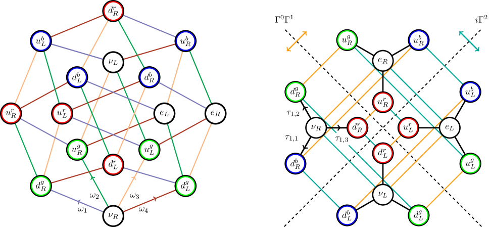
Figure 1: Left: right-multiplying the $\nu_{R}$ ideal $V_{1}$ by combinations of $\omega^{\alpha}$ leads to all possible flavours (up to a sign). Upwards direction is associated to multiplication by $\omega^{\alpha}$ and downwards by $\omega^{\dagger\alpha}$. Right: an alternative graph is obtained by right multiplication with combinations of spacetime vectors $\Gamma^{0}\Gamma^{1}$ and $i\Gamma^{2}$ (up to a sign) and Witt basis vectors $\tau_{\alpha,a}$ defined via $V_{1}\tau_{\alpha,a}=\Omega_{(a)}\omega^{\alpha}$ (c.f. Sec. II of the Appendix). The doublet and triplet structures of the weak and strong force become evident. Each colour can be obtained from the center of the triplet structure by defining appropriate $\tau_{\alpha,a}$ for each triplet.

V Conclusions

We showed that the entire SM can be obtained from the free Dirac Lagrangian in 8-dimensional space. The three particles families arise as a direct consequence of triality, leading to a generalized Dirac equation containing a mass matrix whose hierarchy obeys a generalized Koide formula. Although the two angles $(\chi,\delta)$ parameterizing the mass matrix remain free at this point, the families in each flavour must obey the specific pattern of Eq. (28). While we know that $(\pi/4,2/9)$ fits the experimental data for the flavour set $(m_{e},m_{\mu},m_{\tau})$ with great precision, obtaining the transcendental angle $\delta=2/9$ fro first principles remains a daunting task. An answer to this question will most likely lead to a complete understanding of the mass matrix and to family mixing.

Although $\mathcal{C}\ell_{8,0}$ strongly indicates the existence of 8-dimensions, we have tacitly avoided details of the higher dimensional metric. It is unknown if the extra dimensions are spacelike, timelike or a mixture of both. The emergence of three particle families is also directly tied to the existence of three orthogonal 4-dimensional spacetimes within a single 8-dimensional space but we provide no mechanism for dimensional reduction. This will likely have an impact on quantum fields (defined in 4-dimensions), allowing the existence of new higher dimensional terms in the Lagrangian. Furthermore, all fermionic representations have been exhausted so no new fermions are expected to be detected (apart from right-handed neutrinos). The bosonic sector, on the other hand, is still not fully understood. While we found that the Higgs doublet sits on a 4-vector-like representation (as indicated by $\Gamma^{2}$), there are no restrictions to bosonic fields apart from possibly having to be represented by similar structures involving $\Gamma^{\mu}$. For example, the mass matrix (27) displays a $[U(1)]^{4}$ symmetry due to the invariance under $\omega^{\alpha}\to e^{i\theta_{\alpha}}\omega^{\alpha}$ transformations, so additional bosonic multiplets might exist with a potential invariant under this symmetry (c.f. Koide:2005 for a similar related model involving a $\mathbb{Z}_{4}$ symmetry).

Coupling unification is also not achieved yet, since the newly predicted particle content includes only singlets under the SM group, leading to the beta functions of the SM, which are known not to exhibit a full intersection of couplings at the unification scale. However, the possible existence of higher order Lagrangian terms compatible with 8-dimensional space as well as additional bosons may correct this issue.

Finally, we note that gravity can be incorporated through local gauge invariance of Lorentz transformations (32) via left multiplication in $\omega^{\dagger\alpha}\Omega^{\dagger}_{(a)}V_{A}$, following a similar approach to Lasenby:1998 . Nevertheless, while Lorentz and gauge transformations are unified as elements in the same algebra, the latter approach applied to SGUT does not represent a unification with gravity since the gravitational (external) degrees of freedom continue to be separated from the gauge (internal) degrees of freedom.

VI Acknowledgements

I thank the support from Fundação para a Ciência e a Tecnologia, through projects CEECIND/02474/2018, 2024.04456.CERN and FCT-Mobility/1312232346/2024-25. I also thank everyone who gave useful feedback in an earlier version of the paper, leading to a more complete state-of-the-art review. In particular, I thank Niels Gresnigt for pointing out to me reference Zenczykowski:2015 . Lastly, I thank Filipe Joaquim for fruitful discussions regarding GUTs.

Appendix for “Spacetime Grand Unified Theory”

I. Explicit construction of fermionic quantum fields using elements of $\mathcal{C}\ell_{8,0}$

In this sction we prove for the first time that fermionic quantum fields can be constructed as infinite tensor products of $\mathcal{C}\ell_{8,0}$ algebras. For convenience, we begin by introducing the following basis $\{e_{A}\}\,(A=1,\ldots,8)$ for $\mathcal{C}\ell_{8,0}$

$$\sum^{8}_{A=1}c_{A}e_{A} =\left(\begin{array}[]{cccccccccccccccc}0&0&-ic_{1}&0&0&0&0&-ic_{2}&-ic_{3}&0&0&0&-ic_{4}&0&0&0\\ 0&0&0&-ic_{1}&0&0&ic_{2}&0&0&-ic_{3}&0&0&0&ic_{4}&0&0\\ ic_{1}&0&0&0&0&-ic_{2}&0&0&0&0&ic_{3}&0&0&0&ic_{4}&0\\ 0&ic_{1}&0&0&ic_{2}&0&0&0&0&0&0&ic_{3}&0&0&0&-ic_{4}\\ 0&0&0&-ic_{2}&0&0&-ic_{1}&0&-ic_{4}&0&0&0&ic_{3}&0&0&0\\ 0&0&ic_{2}&0&0&0&0&-ic_{1}&0&ic_{4}&0&0&0&ic_{3}&0&0\\ 0&-ic_{2}&0&0&ic_{1}&0&0&0&0&0&ic_{4}&0&0&0&-ic_{3}&0\\ ic_{2}&0&0&0&0&ic_{1}&0&0&0&0&0&-ic_{4}&0&0&0&-ic_{3}\\ ic_{3}&0&0&0&ic_{4}&0&0&0&0&0&-ic_{1}&0&0&0&0&ic_{2}\\ 0&ic_{3}&0&0&0&-ic_{4}&0&0&0&0&0&-ic_{1}&0&0&-ic_{2}&0\\ 0&0&-ic_{3}&0&0&0&-ic_{4}&0&ic_{1}&0&0&0&0&ic_{2}&0&0\\ 0&0&0&-ic_{3}&0&0&0&ic_{4}&0&ic_{1}&0&0&-ic_{2}&0&0&0\\ ic_{4}&0&0&0&-ic_{3}&0&0&0&0&0&0&ic_{2}&0&0&-ic_{1}&0\\ 0&-ic_{4}&0&0&0&-ic_{3}&0&0&0&0&-ic_{2}&0&0&0&0&-ic_{1}\\ 0&0&-ic_{4}&0&0&0&ic_{3}&0&0&ic_{2}&0&0&ic_{1}&0&0&0\\ 0&0&0&ic_{4}&0&0&0&ic_{3}&-ic_{2}&0&0&0&0&ic_{1}&0&0\\ \end{array}\right)$$ (A17)

$$+\left(\begin{array}[]{cccccccccccccccc}0&0&-c_{8}&0&0&0&0&-c_{7}&-c_{6}&0&0&0&-c_{5}&0&0&0\\ 0&0&0&c_{8}&0&0&-c_{7}&0&0&c_{6}&0&0&0&-c_{5}&0&0\\ -c_{8}&0&0&0&0&-c_{7}&0&0&0&0&c_{6}&0&0&0&c_{5}&0\\ 0&c_{8}&0&0&-c_{7}&0&0&0&0&0&0&-c_{6}&0&0&0&c_{5}\\ 0&0&0&-c_{7}&0&0&-c_{8}&0&c_{5}&0&0&0&-c_{6}&0&0&0\\ 0&0&-c_{7}&0&0&0&0&c_{8}&0&c_{5}&0&0&0&c_{6}&0&0\\ 0&-c_{7}&0&0&-c_{8}&0&0&0&0&0&-c_{5}&0&0&0&c_{6}&0\\ -c_{7}&0&0&0&0&c_{8}&0&0&0&0&0&-c_{5}&0&0&0&-c_{6}\\ -c_{6}&0&0&0&c_{5}&0&0&0&0&0&-c_{8}&0&0&0&0&c_{7}\\ 0&c_{6}&0&0&0&c_{5}&0&0&0&0&0&c_{8}&0&0&c_{7}&0\\ 0&0&c_{6}&0&0&0&-c_{5}&0&-c_{8}&0&0&0&0&c_{7}&0&0\\ 0&0&0&-c_{6}&0&0&0&-c_{5}&0&c_{8}&0&0&c_{7}&0&0&0\\ -c_{5}&0&0&0&-c_{6}&0&0&0&0&0&0&c_{7}&0&0&-c_{8}&0\\ 0&-c_{5}&0&0&0&c_{6}&0&0&0&0&c_{7}&0&0&0&0&c_{8}\\ 0&0&c_{5}&0&0&0&c_{6}&0&0&c_{7}&0&0&-c_{8}&0&0&0\\ 0&0&0&c_{5}&0&0&0&-c_{6}&c_{7}&0&0&0&0&c_{8}&0&0\\ \end{array}\right)\,,$$ (A34)

from which a Witt basis shall be constructed shortly. We now discretize the spatial dimensions of spacetime, without loss of generality, as a cubic lattice in 3 spatial dimensions with length $L$, volume $V=L^{3}$ and lattice spacing $a$. In momentum space, this corresponds to discretizing momentum into $(L/a)^{3}$ modes, labelled $\textbf{p}_{I}$ with $I=(i_{1},i_{2},i_{3})$ $(i_{n}\in\mathbb{Z})$, distributed with spacing $2\pi/L$. In turn, this induces the discretization of the creation-annihilation operators, resulting in the new anticommutation relations

$$\{a^{s}_{\textbf{p}_{I}},a^{r\dagger}_{\textbf{p}_{J}}\} =\{b^{s}_{\textbf{p}_{I}},b^{r\dagger}_{\textbf{p}_{J}}\}=L^{3}\delta^{sr}\delta_{i_{1}j_{1}}\delta_{i_{2}j_{2}}\delta_{i_{3}j_{3}}\,,$$ (A35)

$$\{a^{s}_{\textbf{p}_{I}},a^{r}_{\textbf{k}_{J}}\} =\{a^{s\dagger}_{\textbf{p}_{I}},a^{r\dagger}_{\textbf{k}_{J}}\}=\{b^{s}_{\textbf{p}_{I}},\hat{b}^{r}_{\textbf{k}_{J}}\}=\{b^{s\dagger}_{\textbf{p}_{I}},b^{r\dagger}_{\textbf{k}_{J}}\}=0\,,$$ (A36)

where the hat notation disappears since the creation operators are now finite matrices. The anticommutation relations (A35) and (A36) correspond to a Witt basis of some Clifford algebra. To identify the latter algebra, we focus on a Witt basis $\{\omega^{\alpha}\}$ for a Clifford algebra whose anticommutation relations satisfy Eq. (5). There is a well-established literature on how to build Witt bases and the properties of such objects (see Lounesto:2001 for a modern take and references therein). For the specific case of Eq. (5), the lowest dimensional representation for $\omega^{a}$ are $16\times 16$ matrices belonging to $\mathcal{C}\ell_{8,0}$ with multiple possible metric signatures, i.e. $\mathcal{C}\ell_{l,n}$ such that $l+n=8$. Without loss of generality, we will take $\omega^{a}\in\mathcal{C}\ell_{8,0}$, which can be constructed from Eq. (A34) and Eq. (6), leading to

$$\sum^{4}_{\alpha=1}c_{\alpha}\omega^{\alpha}=\left(\begin{array}[]{cccccccccccccccc}0&0&c_{1}&0&0&0&0&c_{2}&c_{3}&0&0&0&c_{4}&0&0&0\\ 0&0&0&0&0&0&0&0&0&0&0&0&0&0&0&0\\ 0&0&0&0&0&c_{2}&0&0&0&0&-c_{3}&0&0&0&-c_{4}&0\\ 0&-c_{1}&0&0&0&0&0&0&0&0&0&0&0&0&0&0\\ 0&0&0&c_{2}&0&0&c_{1}&0&0&0&0&0&0&0&0&0\\ 0&0&0&0&0&0&0&0&0&-c_{4}&0&0&0&-c_{3}&0&0\\ 0&c_{2}&0&0&0&0&0&0&0&0&0&0&0&0&0&0\\ 0&0&0&0&0&-c_{1}&0&0&0&0&0&c_{4}&0&0&0&c_{3}\\ 0&0&0&0&-c_{4}&0&0&0&0&0&c_{1}&0&0&0&0&-c_{2}\\ 0&-c_{3}&0&0&0&0&0&0&0&0&0&0&0&0&0&0\\ 0&0&0&0&0&0&c_{4}&0&0&0&0&0&0&-c_{2}&0&0\\ 0&0&0&c_{3}&0&0&0&0&0&-c_{1}&0&0&0&0&0&0\\ 0&0&0&0&c_{3}&0&0&0&0&0&0&-c_{2}&0&0&c_{1}&0\\ 0&c_{4}&0&0&0&0&0&0&0&0&0&0&0&0&0&0\\ 0&0&0&0&0&0&-c_{3}&0&0&-c_{2}&0&0&0&0&0&0\\ 0&0&0&-c_{4}&0&0&0&0&0&0&0&0&0&-c_{1}&0&0\\ \end{array}\right)\,.$$ (A37)

The elements $\omega^{\alpha\dagger}$ are obtained by hermitian conjugation. The algebra $\mathcal{C}\ell_{8,0}$ plays a special role in the theory of Clifford algebras thanks to a theorem due to Cartan Cartan:1908 , also commonly referred to as Bott periodicity. The latter result states that $\mathcal{C}\ell_{l,n+8}\simeq\mathcal{C}\ell_{l,n}\otimes\mathcal{C}\ell_{0,8}$ or $\mathcal{C}\ell_{l+8,n}\simeq\mathcal{C}\ell_{l,n}\otimes\mathcal{C}\ell_{8,0}$, or in other words, any element from a Clifford algebra with dimension greater than 8 can be written as a tensor product of $\mathcal{C}\ell_{8,0}$ and another Clifford algebra. This property allows us to write any element of the Witt basis $\{\Xi^{i}\}$ of $\mathcal{C}\ell_{8N,0}$ $(N\in\mathbb{N}^{+})$ as the tensor product of Witt basis elements of $\mathcal{C}\ell_{8,0}$. In particular, one can construct the basis

$$\{\Xi^{i}\} =\{\omega^{s_{1}}\otimes I_{e}\otimes\cdots\otimes I_{e},1_{16\times 16}\otimes\omega^{s_{2}}\otimes I_{e}\otimes\cdots\otimes I_{e},\ldots,1_{16\times 16}\otimes\cdots\otimes 1_{16\times 16}\otimes\omega^{s_{N}}\}$$ (A38)

where $s_{k}=1,\ldots,4$, each $\omega^{s_{k}}$ obeys the commutation rules of Eq. (5), $I_{e}\equiv e_{1}\ldots e_{8}$ and each $\Xi^{i}$ is a $16^{N}$-dimensional matrix. It is straightforward to check that the $4N$ elements $\Xi^{i}$ satisfy the required commutation relations for a Witt basis of $\mathcal{C}\ell_{8N,0}$, i.e. $\{\Xi^{i},\Xi^{j\dagger}\}=\delta^{ij}$, $\{\Xi^{i},\Xi^{j}\}=\{\Xi^{i\dagger},\Xi^{j\dagger}\}=0$, where $i,j=1,\ldots,N$. Using the latter relations together with Eq. (5), one obtains the correspondence

$$a^{1}_{\textbf{p}_{I}} \equiv L^{3/2}(\omega^{1}\otimes\Xi^{i_{1}}\otimes\Xi^{i_{2}}\otimes\Xi^{i_{3}})\,,$$ (A39)

$$a^{2}_{\textbf{p}_{I}} \equiv L^{3/2}(\omega^{2}\otimes\Xi^{i_{1}}\otimes\Xi^{i_{2}}\otimes\Xi^{i_{3}})\,,$$ (A40)

$$b^{1}_{\textbf{p}_{I}} \equiv L^{3/2}(\omega^{3}\otimes\Xi^{i_{1}}\otimes\Xi^{i_{2}}\otimes\Xi^{i_{3}})\,,$$ (A41)

$$b^{2}_{\textbf{p}_{I}} \equiv L^{3/2}(\omega^{4}\otimes\Xi^{i_{1}}\otimes\Xi^{i_{2}}\otimes\Xi^{i_{3}})\,,$$ (A42)

obeying precisely the commutation relations of Eqs. (A35)-(A36). In the limit $N\to\infty$, one recovers the continuous infinite dimensional anticommutation relations (3) and (4) and so $a^{s}_{\textbf{p}_{I}}\to\hat{a}^{s}_{\textbf{p}}$ and $b^{s}_{\textbf{p}_{I}}\to\hat{b}^{s}_{\textbf{p}}$ in that limit. We thus prove that one may consider $\hat{a}^{s}_{\textbf{p}},\hat{b}^{s}_{\textbf{p}}\in\mathcal{C}\ell_{8,0}\otimes\lim_{N\to\infty}(\mathcal{C}\ell_{8N,0})^{\otimes 3}$ and, since the discretized quantum field is a linear combination of creation and annihilation operators, we also have that $\hat{\psi}_{\alpha}(x)\in\mathcal{C}\ell_{8,0}\otimes\lim_{N\to\infty}(\mathcal{C}\ell_{8N,0})^{\otimes 3}$. In particular, since the quantized momentum modes are also generated by $\omega^{\alpha}$ matrices due to Eq. (A38), one may use the property $\omega^{\alpha}V_{i}=0$ to conclude that the full quantum field vacuum in the continuous limit can be written as $\ket{0}=V_{i}\otimes\lim_{N\to\infty}V_{i}^{\otimes 3N}$. While it has been frequently remarked in the literature that $V_{1}$ has the analogous properties of a vacuum, this is the first time that the actual quantum field vacuum $\ket{0}$ has been expressed as a functional of $V_{1}$ (or $V_{i}$ more generally). Having access to Eq. (A37) we can now find the form of a general rest frame spinor via Eqs. (10)-(13), in the form

$$c_{s}u^{s}_{16D}(0)+d_{s}v^{s}_{16D}(0)=\left\{\begin{array}[]{ll}(0,0,c_{1},0,0,0,0,c_{2},d_{1},0,0,0,d_{2},0,0,0)^{T},\textrm{ for column}\,\,i\\ 0,\textrm{ otherwise.}\\ \end{array}\right.\,.$$ (A43)

II. Spin(8) triality in $\mathcal{C}\ell_{8,0}$

Among the representations of the Spin($n$) group, there are three of special relevance for this work: two spinorial ones, denoted by $S_{\pm}$ and a vectorial one, denoted by $V$. For the majority of $n$, these representations don’t have the same dimensions. However, for $n=8$, all the dimensions are equal to 8 and so any two elements of different representations uniquely define a third one in the remaining representation - a phenomenon called triality. Rather than give an exposition on triality, which can get unnecessarily technical, we shall only use the results from Lounesto:2001 which will be required for this work. Note that, since all basis matrices are explicitly stated, all results presented here can be straightforwardly verified using a symbolic manipulation software such as Mathematica.

Consider then an element of the vector space of $\mathcal{C}\ell_{8,0}$, here denoted by $\mathcal{V}$, i.e. an element of the form $v=v^{A}e_{A}$. Let $s^{(0)}\in\mathcal{C}\ell_{8,0}$ be an even product of normalized vectors, i.e. of the form $s^{(0)}=v_{(1)}v_{(2)}\dots v_{(2r)}$ where $v_{(k)}\in\mathcal{V}$ are vectors such that $v_{(k)}v_{(k)}\equiv(v_{(k)})^{2}=1$. Then $s^{(0)}$ will rotate the vector $v$ into a new vector $g_{(0)}(v)$ via the action

$$g_{(0)}(v)=s^{(0)}v(s^{(0)})^{-1}\in\mathcal{V}\,,$$ (A44)

where $g_{(0)}$ is an element of the vector representation $V$ of Spin(8) expressed in the space of $\mathcal{C}\ell_{8,0}$. Now take a vector $n\in\mathcal{V}$ and an element $w\in\mathcal{C}\ell_{8,0}$, made of linear combinations of elements of the form $e_{A}e_{B}e_{C}e_{D}$, such that

$$n^{2}=1\,,\quad w^{2}=7+6w\,,\quad[w,n]=0\,.\\$$ (A45)

We can generate two independent spinor spaces $\mathcal{S}_{\pm}$ via Lounesto:2001

$$\mathcal{S}_{\pm}=\mathcal{C}\ell^{+}_{8,0}\left(\frac{1+w}{8}\right)\left(\frac{1\pm I_{e}}{2}\right)\,,$$ (A46)

where $\mathcal{C}\ell^{+}_{8,0}$ denotes the even subspace of $\mathcal{C}\ell_{8,0}$, i.e. all elements made of even products. Elements $g_{(\pm)}$ of Spin(8) in the spinor representations $S_{\pm}$ will act in the form

$$g_{(\pm)}(\mathcal{S}_{\pm})=s^{(\pm)}\mathcal{C}\ell^{+}_{8,0}\left(\frac{1+w}{8}\right)\left(\frac{1\pm I_{e}}{2}\right)\,,$$ (A47)

where $s^{(\pm)}$ are elements made of an even product of normalized vectors, similarly to $s^{(0)}$. Note that, since $s^{(\pm)}\in\mathcal{C}\ell^{+}_{8,0}$, then also $s^{(\pm)}\mathcal{C}\ell^{+}_{8,0}\in\mathcal{C}\ell^{+}_{8,0}$ and so $g_{(\pm)}(\mathcal{S}_{\pm})\in\mathcal{S}_{\pm}$ is also a spinor. The action in Eq. (A47) thus represents a rotation of spinors in the spaces $\mathcal{S}_{\pm}$.

The fact that $s^{(0)}$ and $s^{(\pm)}$ all have dimensions equal to 8 means that some relation among rotations in $\mathcal{V}$ and $\mathcal{S}_{\pm}$ should exist. This is in fact true and can be compactly expressed as Lounesto:2001

$$\kappa^{(0)}v(\kappa^{(0)})^{-1}=\braket{u^{(\pm)}v(1+w)(1\pm I_{e})}_{1}$$ (A48)

where $v\in\mathcal{V}$, $\kappa^{(0)}$ is a spinor, $\braket{x}_{1}$ denotes the vector part of $x\in\mathcal{C}\ell_{8,0}$ (i.e. the component of $x$ which can be written as a linear combination of $e_{A}$) and

$$\kappa^{(-)} =\textrm{trial}(n\kappa^{(0)}n)\,,$$ (A49)

$$\kappa^{(+)} =\textrm{trial}(\textrm{trial}(n\kappa^{(0)}n))$$ (A50)

where trial is the triality operation, defined as (for $u=v_{(1)}\ldots v_{(2r)}$ and $v^{2}_{(i)}=1$)

$$\textrm{trial}(u) =\bigg{[}\left(\frac{1+I_{e}}{2}\right)\{\braket{u(1+w)(1-I_{e})}_{0,6},n\}n$$

$$\hskip-22.76219pt+\left(\frac{1-I_{e}}{2}\right)\bigg{]}(w-3)\{u(1+I_{e}),n\}n(w-3)^{-1}\,,$$ (A51)

where $\braket{x}_{0,6}\equiv\braket{x}_{0}+\braket{x}_{6}$ represents the summation of the scalar part of $x\in\mathcal{C}\ell_{8,0}$ and the component made of linear combinations of $e_{A}e_{B}e_{C}e_{D}e_{E}e_{F}$. The triality operation, as the name suggests, obeys the property ${\textrm{trial}(\textrm{trial}(\textrm{trial}(u)))=u}$ for any spinor $u$. Eq. (A48) essentially states that the rotation of a vector in 8-dimensional space can be viewed in exactly 3 equivalent ways, expressed as rotations in 3 distinct Spin(8) representations. The objects $w$ and $n$ obeying Eq. (A45) are known as calibration and the neutral axis of the calibration, respectively, and together uniquely define an octonionic product via

$$a\circ b=\braket{anb(1+w)(1-I_{e})}_{1}$$ (A52)

where $a,b\in\mathcal{V}$ and $\braket{\hskip 5.69054pt}_{1}$ is the part proportional to a linear combination of $e_{A}$ Lounesto:2001 . Using the fact that Lounesto:2001

$$\braket{x}_{1}=\braket{xe_{A}}_{0}e_{A}=\frac{1}{16}\textrm{Tr}[xe_{A}]e_{A}$$ (A53)

and

$$\textrm{Tr}[e_{A}e_{B}]=16\,\delta_{AB}\,,$$ (A54)

one can obtain an alternative form of Eq. (A48) by considering $v=e_{A}$, multiplying by $e_{B}$ from the right and taking the trace, resulting in

$$\textrm{Tr}\left[\frac{\kappa^{(0)}e_{A}(\kappa^{(0)})^{-1}e_{B}}{16}\right]=\textrm{Tr}\left[\kappa^{(\pm)}e_{A}\left(\frac{1+w}{8}\right)\left(\frac{1\pm I_{e}}{2}\right)e_{B}\right]\,.$$ (A55)

We can now explore the consequences of Eq. (A48) for the matrix components of a Dirac algebra element $X_{\alpha\beta}$ by taking the explicit calibration

$$w =e_{1}e_{2}e_{3}e_{4}+e_{1}e_{4}e_{6}e_{7}-e_{1}e_{3}e_{5}e_{7}+e_{1}e_{2}e_{5}e_{6}-e_{3}e_{4}e_{5}e_{6}-e_{2}e_{4}e_{5}e_{7}-e_{2}e_{3}e_{6}e_{7}$$ (A56)

$$=\begin{pmatrix}3&-4&0&0\\ -4&3&0&0\\ 0&0&3&4\\ 0&0&4&3\\ \end{pmatrix}\oplus(-1_{12\times 12})$$ (A57)

and its neutral axis

$$n=e_{8}$$ (A58)

from which one may derive the identity

$$\omega^{\alpha}P_{(+)}=-2\,n\omega^{1\dagger}\left(\frac{1+w}{8}\right)\left(\frac{1+I_{e}}{2}\right)\omega^{\alpha}\,.$$ (A59)

The above relation will change according to different choices of neural axis, although such change will amount to switching $\omega^{1\dagger}$ for another vector without consequence for any of the results from this work. Inserting the above relation in Eq. (19) and using ${(1+w)(1+I_{e})\omega^{1}\omega^{1\dagger}(1+w)(1+I_{e})=8(1+w)(1+I_{e})}$ together with $\omega^{\alpha\dagger}V_{1}=P_{(+)}\omega^{\alpha\dagger}$ and Eq. (A59), one obtains

$$X_{\alpha\beta}=(\omega^{\alpha})^{B}(\omega^{\beta\dagger})^{A}\textrm{Tr}\left[X_{(\omega)}e_{A}\left(\frac{1+w}{8}\right)\left(\frac{1+I_{e}}{2}\right)e_{B}\right]\,,$$ (A60)

where we pulled the Witt basis coefficients out of the trace for future convenience. We now focus on a specific class of Dirac matrices $N_{\alpha\beta}$ such that

$$N_{\alpha\nu}N_{\nu\beta}=\delta_{\alpha\beta}\,,$$ (A61)

of which $\gamma^{0}$ and $\gamma^{0}\gamma^{\mu}$ appearing in the Lagrangian are examples of interest. For this class of matrices, one finds through Eq. (18) that

$$P_{(+)}N_{(\omega)}P_{(+)}=P_{(+)}\left(-ie^{i\frac{\pi}{2}N_{(\omega)}}\right)P_{(+)}\equiv-iP_{(+)}u^{(+)}P_{(+)}$$ (A62)

where $u^{(+)}$ is a spinor (since it is an exponential of combinations of $e_{A}e_{B}$ Lounesto:2001 ). Consequently, using (A55), (A60), (A62) and $\omega^{\alpha\dagger}V_{1}=P_{(+)}\omega^{\alpha\dagger}$, we find that

$$N_{\alpha\beta} =-2i\,\textrm{Tr}\left[\frac{u^{(0)}\omega^{\dagger\beta}(u^{(0)})^{-1}\omega^{\alpha}}{16}\right]$$ (A63)

$$=-2i\,\textrm{Tr}\left[u^{(\pm)}\omega^{\beta\dagger}\left(\frac{1+w}{8}\right)\left(\frac{1\pm I_{e}}{2}\right)\omega^{\alpha}\right]$$ (A64)

where we have ${u^{(-)}=n\textrm{trial}(nu^{(+)}n)}n$ and ${u^{(0)}=\textrm{trial}(\textrm{trial}(nu^{(+)}n))}$. In other words, we observe that there are exactly three ways to embed $N_{\alpha\beta}$ within the algebra $\mathcal{C}\ell_{8,0}$ once a calibration $w$ and a neutral axis $n$ are chosen, i.e. once an orientation in 8-dimensional space (or octonionic product) is defined. The appearance of Eqs. (A63)-(A64) can be made more uniform by first defining

$$\Omega_{(+)}\equiv\sqrt{2}n\,\omega^{1\dagger}\left(\frac{1+w}{8}\right)\left(\frac{1+I_{e}}{2}\right)=\frac{1}{\sqrt{2}}\begin{pmatrix}-1&1\\ 0&0\end{pmatrix}\oplus(0_{14\times 14})$$ (A65)

which appears naturally in Eq. (A59) and where $0_{n\times n}$ denotes the n-dimensional square zero matrix. The quantity $\Omega_{(+)}$ satisfies the relations

$$\omega^{\alpha}\Omega_{(+)}=0\,,\quad\omega^{\alpha\dagger}\Omega_{(+)}\neq 0\,,$$ (A66)

so it is interpreted as a vacuum for the creation operators $\omega^{\alpha\dagger}$. This is in fact expected since it also satisfies

$$(\Omega^{\dagger}_{(+)}\Omega_{(+)})^{2}=\Omega^{\dagger}_{(+)}\Omega_{(+)}\,,\quad\Omega_{(+)}\Omega^{\dagger}_{(+)}=V_{1}\,,$$ (A67)

which implies that $\omega^{\alpha}V_{1}=0$ can be obtained from Eq. (A66) by left multiplication with $\Omega^{\dagger}_{(+)}$. Taking inspiration from Eq. (A65), one can search from an analogous object in the spinor space $\mathcal{S}_{-}$ such that Eq. (A67) is still valid with a different index. The unique object that satisfies such properties is given by

$$\Omega_{(-)}\equiv\sqrt{2}\,\omega^{1}\left(\frac{1+w}{8}\right)\left(\frac{1-I_{e}}{2}\right)=\frac{1}{\sqrt{2}}\begin{pmatrix}0&0&1&1\\ 0&0&0&0\\ 0&0&0&0\\ 0&0&0&0\end{pmatrix}\oplus(0_{12\times 12})\,.$$ (A68)

The latter vacuum shares a set of properties with $\Omega_{(+)}$, namely

$$\Omega^{\dagger}_{(\pm)}\Omega_{(\pm)}=\left(\frac{1+w}{8}\right)\left(\frac{1\pm I_{e}}{2}\right)\,,$$ (A69)

$$\textrm{Tr}[e_{A}e_{B}\Omega^{\dagger}_{(\pm)}\Omega_{(\pm)}]=\delta_{AB}\,.$$ (A70)

In particular, Eq. (A69) allows one to write Eq. (A64) as

$$N_{\alpha\beta}=-2i\,\textrm{Tr}\left[\Omega_{(\pm)}\omega^{\alpha}u^{(\pm)}\omega^{\beta\dagger}\Omega^{\dagger}_{(\pm)}\right]\,.$$ (A71)

It would now be most convenient if one could express (A63) in the same form as (A71). Although this appears to be impossible for general $u^{(0)}$, one may focus on the explicit cases at hand, namely $(\gamma^{0}\gamma^{\mu})_{\alpha\beta}$ and $(\gamma^{0})_{\alpha\beta}$. This implies that Eq. (A63) will just be applied to ${u^{\mu}_{(0)}\equiv\textrm{trial}(\textrm{trial}(n(\gamma^{0}\gamma^{\mu})_{\alpha\beta}\omega^{\alpha\dagger}\omega^{\beta}n)})$ and ${\kappa_{(0)}\equiv\textrm{trial}(\textrm{trial}(n(\gamma^{0})_{\alpha\beta}\omega^{\alpha\dagger}\omega^{\beta}n)})$. We can now search for a vacuum $\Omega_{(0)}$ which, in addition to satisfying Eqs. (A66) and (A70), also obeys

$$(u^{\mu}_{(0)})^{-1}\Omega^{\dagger}_{(0)} =\Omega^{\dagger}_{(0)}\,,$$ (A72)

$$(\kappa_{(0)})^{-1}\Omega^{\dagger}_{(0)} =\Omega^{\dagger}_{(0)}\,.$$ (A73)

One can show that the unique solution for this is

$$\Omega^{(0)}=\frac{1}{\sqrt{2}}\omega^{1}\omega^{2}\omega^{3}\omega^{4}(\omega^{1\dagger}\omega^{2\dagger}-\omega^{3\dagger}\omega^{4\dagger})=\frac{1}{\sqrt{2}}\begin{pmatrix}0&0&0&0&1&1\\ 0&0&0&0&0&0\\ 0&0&0&0&0&0\\ 0&0&0&0&0&0\\ 0&0&0&0&0&0\\ 0&0&0&0&0&0\end{pmatrix}\oplus(0_{10\times 10})\,,$$ (A74)

which, using Eqs. (A63), (A70) and (A71), leads to

$$(\gamma^{0}\gamma^{\mu})_{\alpha\beta} =-2i\,\textrm{Tr}\left[\Omega_{(a)}\omega^{\alpha}u^{\mu}_{(a)}\omega^{\beta\dagger}\Omega^{\dagger}_{(a)}\right]\,,$$ (A75)

$$(\gamma^{0})_{\alpha\beta} =-2i\,\textrm{Tr}\left[\Omega_{(a)}\omega^{\alpha}\kappa_{(a)}\omega^{\beta\dagger}\Omega^{\dagger}_{(a)}\right]\,,$$ (A76)

where $a\in\{+,-,0\}$. Finally, it would be ideally elegant to find that the representation index in $u^{\mu}_{(a)}$ and $\kappa_{(a)}$ can be removed by using instead a set of four matrices $\Gamma^{\mu}\in C\ell_{8,0}$ in the traces of Eqs. (A75)-(A76), for all vacua. This is in fact possible with the following set:

$$\sum^{3}_{\mu=0}c_{\mu}\Gamma^{\mu} =\left(\begin{array}[]{cccccccccccccccc}0&0&0&0&0&0&0&0&0&0&0&c_{0}&0&0&0&c_{1}\\ 0&0&0&0&0&0&0&0&0&0&c_{0}&0&0&0&c_{1}&0\\ 0&0&0&0&0&0&0&0&c_{0}&0&0&0&c_{1}&0&0&0\\ 0&0&0&0&0&0&0&0&0&-c_{0}&0&0&0&-c_{1}&0&0\\ 0&0&0&0&0&0&0&0&0&0&0&c_{1}&0&0&0&c_{0}\\ 0&0&0&0&0&0&0&0&0&0&-c_{1}&0&0&0&-c_{0}&0\\ 0&0&0&0&0&0&0&0&0&-c_{1}&0&0&0&-c_{0}&0&0\\ 0&0&0&0&0&0&0&0&c_{1}&0&0&0&c_{0}&0&0&0\\ 0&0&c_{0}&0&0&0&0&-c_{1}&0&0&0&0&0&0&0&0\\ 0&0&0&-c_{0}&0&0&c_{1}&0&0&0&0&0&0&0&0&0\\ 0&c_{0}&0&0&0&c_{1}&0&0&0&0&0&0&0&0&0&0\\ c_{0}&0&0&0&-c_{1}&0&0&0&0&0&0&0&0&0&0&0\\ 0&0&-c_{1}&0&0&0&0&c_{0}&0&0&0&0&0&0&0&0\\ 0&0&0&c_{1}&0&0&-c_{0}&0&0&0&0&0&0&0&0&0\\ 0&-c_{1}&0&0&0&-c_{0}&0&0&0&0&0&0&0&0&0&0\\ -c_{1}&0&0&0&c_{0}&0&0&0&0&0&0&0&0&0&0&0\\ \end{array}\right)$$ (A93)

$$+\left(\begin{array}[]{cccccccccccccccc}0&0&0&0&0&0&0&0&0&0&0&c_{3}&0&0&0&-ic_{2}\\ 0&0&0&0&0&0&0&0&0&0&c_{3}&0&0&0&-ic_{2}&0\\ 0&0&0&0&0&0&0&0&c_{3}&0&0&0&-ic_{2}&0&0&0\\ 0&0&0&0&0&0&0&0&0&c_{3}&0&0&0&-ic_{2}&0&0\\ 0&0&0&0&0&0&0&0&0&0&0&ic_{2}&0&0&0&-c_{3}\\ 0&0&0&0&0&0&0&0&0&0&-ic_{2}&0&0&0&c_{3}&0\\ 0&0&0&0&0&0&0&0&0&ic_{2}&0&0&0&-c_{3}&0&0\\ 0&0&0&0&0&0&0&0&ic_{2}&0&0&0&-c_{3}&0&0&0\\ 0&0&-c_{3}&0&0&0&0&ic_{2}&0&0&0&0&0&0&0&0\\ 0&0&0&-c_{3}&0&0&ic_{2}&0&0&0&0&0&0&0&0&0\\ 0&-c_{3}&0&0&0&-ic_{2}&0&0&0&0&0&0&0&0&0&0\\ -c_{3}&0&0&0&ic_{2}&0&0&0&0&0&0&0&0&0&0&0\\ 0&0&-ic_{2}&0&0&0&0&c_{3}&0&0&0&0&0&0&0&0\\ 0&0&0&-ic_{2}&0&0&c_{3}&0&0&0&0&0&0&0&0&0\\ 0&-ic_{2}&0&0&0&-c_{3}&0&0&0&0&0&0&0&0&0&0\\ -ic_{2}&0&0&0&c_{3}&0&0&0&0&0&0&0&0&0&0&0\\ \end{array}\right)\,,$$ (A110)

from which we can obtain

$$(\gamma^{0}\gamma^{\mu})_{\alpha\beta} =2\,\textrm{Tr}\left[\Omega_{(a)}\omega^{\alpha}\Gamma^{0}\Gamma^{\mu}\omega^{\beta\dagger}\Omega^{\dagger}_{(a)}\right]\,,$$

$$(\gamma^{0})_{\alpha\beta} =2\,\textrm{Tr}\left[\Omega_{(a)}\omega^{\alpha}\Gamma^{0}\omega^{\beta\dagger}\Omega^{\dagger}_{(a)}\right]\,,$$

thereby proving Eqs. (20)-(21). Note that the 4-dimensional subspace associated to the projector $P_{\perp}$ does not contribute to the trace in Eqs. (A75)-(A76). Nevertheless, the components of $\Gamma^{\mu}$ associated to this subspace have been fixed to ensure both that $\det(\Gamma^{\mu})=1$ and the correct norms for $\Gamma^{\mu}$.

Finally, in order to reproduce the right hand side of Fig. 1, it proves worthwhile to look for three Witt bases $\{\tau_{\alpha,a}\}$ with $\alpha=1,\ldots,4$ and $a\in\{0,+,-\}$ such that

$$\tau^{\dagger}_{\alpha,a}V_{1}=\omega^{\dagger\alpha}\Omega^{\dagger}_{(a)}\,.$$ (A111)

After some algebraic endeavors, one can arrive at the following solution:

$$\sum_{\alpha,a}c_{\alpha,a}\tau_{\alpha,a}=$$

$$\hskip-25.60747pt\left(\begin{array}[]{cccccccccccccccc}0&-c_{1,-}&-c_{1,+}&-c_{2,0}&0&-c_{2,-}&-c_{1,0}&-c_{2,+}&-c_{3,+}&-c_{4,0}&-c_{3,-}&0&-c_{4,+}&-c_{3,0}&-c_{4,-}&0\\ 0&0&0&0&0&0&0&c_{2,-}&c_{3,-}&0&0&0&0&0&0&-c_{4,-}\\ 0&-c_{2,0}&0&0&c_{1,-}&-c_{2,+}&0&0&0&0&c_{3,+}&0&0&0&c_{4,+}&0\\ 0&c_{1,+}&c_{2,-}&0&0&-c_{1,0}&c_{1,-}&0&0&0&c_{4,0}&0&0&0&c_{3,0}&0\\ 0&0&c_{1,0}&-c_{2,+}&0&0&-c_{1,+}&c_{2,0}&0&0&0&0&0&0&0&0\\ 0&0&0&0&0&0&0&-c_{1,-}&c_{3,0}&c_{4,+}&0&c_{3,-}&c_{4,0}-c_{4,-}&c_{3,+}&0&0\\ 0&-c_{2,+}&0&0&-c_{2,-}&c_{2,0}&0&0&0&0&0&c_{3,0}&0&0&0&c_{4,0}\\ 0&c_{1,0}&0&0&0&c_{1,+}&0&0&0&-c_{4,-}&0&-c_{4,+}&0&-c_{3,-}&0&-c_{3,+}\\ 0&-c_{4,0}&0&0&c_{4,+}&0&c_{4,-}&0&0&0&-c_{1,+}&0&0&c_{2,-}&0&c_{2,+}\\ 0&c_{3,+}&0&0&-c_{3,0}-c_{3,-}&0&0&0&0&0&-c_{2,0}&0&0&0&0&-c_{1,0}\\ 0&0&0&c_{4,-}&0&0&-c_{4,+}&-c_{3,0}&-c_{1,-}&0&0&-c_{2,-}&c_{1,0}&c_{2,+}&0&0\\ 0&0&c_{4,0}+c_{4,-}&-c_{3,+}&0&0&0&0&-c_{2,0}&c_{1,+}&0&0&0&-c_{1,-}&0&0\\ 0&c_{3,0}&c_{3,-}&0&-c_{3,+}&0&0&0&0&c_{1,-}&0&c_{2,+}&0&0&-c_{1,+}&0\\ 0&-c_{4,+}&0&0&c_{4,0}+c_{4,-}&0&0&0&0&0&0&-c_{1,0}&0&0&-c_{2,0}&0\\ 0&0&0&-c_{3,-}&0&0&c_{3,+}&c_{4,0}&c_{1,0}&c_{2,+}&0&0&c_{2,-}&0&0&c_{1,-}\\ 0&0&-c_{3,0}&c_{4,+}&0&0&c_{3,-}&0&0&-c_{2,-}&0&0&-c_{2,0}&c_{1,+}&0&0\\ \end{array}\right)$$ (A128)

As far as the author is aware, all results from Eq. (A60) to Eq. (II. Spin(8) triality in $\mathcal{C}\ell_{8,0}$) are completely novel results in the Clifford algebra literature.

III. General properties of the mass matrix in the family Dirac equation

We begin by noting that the form of the mass matrix $M$ in Eq. (26), namely

$$M=\sum_{\alpha,a,b}M_{ab}\,\omega^{\alpha\dagger}\Omega_{(a)}^{\dagger}\Omega_{(b)}\omega^{\alpha}$$

is a 16-dimensional matrix whose numerical values are dictated by the 3-dimensional matrix $M_{ab}$ and thus so is its eigenvalue spectrum. Consequently, we need only to focus on the properties of $M_{ab}$ to obtain conclusions regarding the mass spectrum. Defining the 3-dimensional matrix $\mathcal{M}$ with components

$$\mathcal{M}_{ab}=iM_{ab}$$ (A129)

it was already observed that $\mathcal{M}$ must be hermitian in order to conserve probabilities in the rest frame, leading to the conclusion that $\mathcal{M}\in\mathfrak{u}(3)$, i.e. it belongs to the Lie algebra of $U(3)$. Now, due to the Cay-Hamilton theorem, any power of $iH\in\mathfrak{u}(3)$ can be expressed as, at most, a second degree polynomial in $H$ Curtright:2015 , so the most general form for $\mathcal{M}$ must necessarily be

$$\mathcal{M}=a1_{3\times 3}+bH+H^{2}\,,\quad a,b\in\mathbb{R}$$ (A130)

such that $\mathcal{M}^{\dagger}=\mathcal{M}$ and where a coefficient for $H^{2}$ is absorbed into its normalization. Since $iH$ always has purely imaginary eigenvalues, the simplest hypothesis which guarantees positive semi-definiteness of the mass spectrum thus corresponds to $a=b=0$, i.e.

$$\mathcal{M}=H^{2}\,,\quad H\in\mathfrak{u}(3)$$ (A131)

with $H$ parametrized through

$$H=q1_{3\times 3}+H^{SU(3)}$$ (A132)

where $q\in\mathbb{R}$ and

$$H^{SU(3)}=\sum^{8}_{k=1}c_{k}\lambda^{SU(3)}_{k}\,,\quad c_{k}\in\mathbb{C}$$ (A133)

and $\lambda^{SU(3)}_{k}$ are the Gell-Mann matrices. It is well known that the eigenvalues of $H^{SU(3)}$ are given by Curtright:2015

$$\frac{2|\textbf{c}|}{\sqrt{3}}\cos\left(\delta+\frac{2\pi k}{3}\right)\,,\quad k=0,1,2$$ (A134)

with $|\textbf{c}|^{2}=\sum^{8}_{k=1}c^{2}_{k}$ and where $\delta$ is an angle uniquely defined by the invariant $\det(H^{SU(3)})$ through the parametric equation

$$\cos(3\delta)=\frac{3\sqrt{3}}{2|\textbf{c}|^{3}}\det(H^{SU(3)})\,.$$ (A135)

We can now define the variables $E$ and $\chi$ via

$$E\sin\chi =\frac{|\textbf{c}|}{\sqrt{2}}$$ (A136)

$$E\cos\chi =\frac{q\sqrt{3}}{2}$$ (A137)

which, upon insertion in Eq. (A132) leads to the general form of its eigenvalues $\varepsilon_{k}$ as

$$\varepsilon_{k}=\frac{2E}{\sqrt{3}}\left(\cos\chi+\sqrt{2}\sin\chi\cos\left(\delta+\frac{2\pi k}{3}\right)\right)\,,\quad k=0,1,2\,.$$ (A138)

At the same time, Eq. (A131) implies that each mass eigenvalue $m_{k}$ is given by $m_{k}=\varepsilon^{2}_{k}$, such that $|\varepsilon_{k}|=\sqrt{m_{k}}$, thereby reproducing Eq. (28). Additionally, since $\textrm{Tr}[\mathcal{M}]=m_{1}+m_{2}+m_{3}$, one can perform the trace of $H^{2}$ using Eq. (A132) and Eq. (A137) to conclude that

$$E=\frac{\sqrt{m_{1}+m_{2}+m_{3}}}{2}\,,$$ (A139)

thus proving Eq. (29). Similarly, performing the trace of Eq. (A132) and using Eqs. (A137) and (29), we obtain

$$\cos\chi=\frac{\sum_{k}\textrm{sign}(\varepsilon_{k})\sqrt{m_{k}}}{\sqrt{3}\sqrt{m_{1}+m_{2}+m_{3}}}$$ (A140)

whose square gives the more familiar form in Eq. (30). Note that the sign of $\varepsilon_{k}$ is a complicated function of $\delta$ and $\chi$ via Eq. (A138). Further relations can be obtained by calculating $\det(\mathcal{M})$ using Eqs. (A131) and (A138) and simultaneously noting that $\det(\mathcal{M})=m_{1}m_{2}m_{3}$, leading to the equation

$$\frac{E^{6}}{27}\left(3\cos\chi+5\cos(3\chi)+4\sqrt{2}\cos(3\delta)\sin^{3}\chi\right)^{2}=m_{1}m_{2}m_{3}\,.$$ (A141)

The above equation can be inverted to give Eq. (31), thereby allowing one to calculate $\delta$ using $\chi$ and the masses $m_{k}$ without having to specify the eight degrees of freedom $c_{k}$. Note that the square on the left hand side of Eq. (A141) is responsible for the $\pm$ in Eq. (31), which can only be found once $\chi$ and the masses $m_{k}$ are specified, similarly to how the sign of $\varepsilon_{k}$ is unspecified. Finally, for general $a$ and $b$ in Eq. (A130), the most general form for $\mathcal{M}$ is still simply a second order polynomial in $\varepsilon_{k}$.

IV. Consequences of Principle 1

In this section we shall show that Principles 1 uniquely implies that the free Dirac Lagrangian must be invariant under actions of the Standard Model group. We shall begin by noting that gauge transformation in the context of $\mathcal{C}\ell_{8,0}$ are represented by unitary transformations of the ideals $V_{A}$ present in the Lagrangian, in the form of

$$V^{\prime}_{A}=UV_{A}U^{-1}$$ (A142)

where

$$U=e^{iH}$$ (A143)

and $H=H^{\dagger}$ is a general hermitian 16-dimensional matrix belonging to the Lie algebra of some group $G$. Firstly, we remark that the identities

$$\hskip 19.91692ptV_{2}=-\sqrt{2}\,\Omega_{(-)}\omega^{1}\,,V_{3}=-\sqrt{2}\,\Omega_{(+)}\omega^{1}\,,V_{4}=\sqrt{2}\,\Omega_{(0)}\omega^{2}\,,V_{6}=\sqrt{2}\,\Omega_{(-)}\omega^{2}\,,V_{7}=\sqrt{2}\,\Omega_{(0)}\omega^{1}\,,V_{8}=-\sqrt{2}\,\Omega_{(+)}\omega^{2}\,,$$

$$V_{9}=-\sqrt{2}\,\Omega_{(+)}\omega^{3}\,,V_{10}=-\sqrt{2}\,\Omega_{(0)}\omega^{4}\,,V_{11}=-\sqrt{2}\,\Omega_{(-)}\omega^{3}\,,V_{13}=-\sqrt{2}\,\Omega_{(+)}\omega^{4}\,,V_{14}=-\sqrt{2}\,\Omega_{(0)}\omega^{3}\,,V_{15}=-\sqrt{2}\,\Omega_{(-)}\omega^{4}\,,$$

collectively imply that, for twelve values of $A\equiv A(\alpha,a)$, we have $V_{A(\alpha,a)}\propto\Omega_{(a)}\omega^{\alpha}$. Following Principle 1, we now wish to find the group $G$ associated to independent rotations of Witt basis and vacua within ideals, i.e. the most general group whose action is of the form

$$V^{\prime}_{A(\alpha,a)}=UV_{A(\alpha,a)}U^{-1}\propto\left(\Omega_{b}(W_{\Omega})^{b}{}_{a}\right)\left(\omega^{\beta}(W_{\omega})^{\beta}{}_{\alpha}\right)\,.$$ (A144)

To find the group $G$, we start by noting that the group of rotations $U$ can be divided into two categories: those which affect the vacua $\Omega_{(a)}$ and those that don’t. We shall denote the latter as $U_{\omega}$ and the former by $U_{\Omega}$. Focusing on $U_{\omega}$ first, we recall that rotations of $\omega^{\alpha}$ are parametrized by the elements of the spin group Spin(8) Lounesto:2001 . The latter group is a particular example of Spin($2n$), a group of dimension $n(2n-1)$ which can be expressed Mohapatra:2003 as an element of a Clifford algebra $\mathcal{C}\ell_{2n,0}$ of the form

$$U=e^{X}\,,\quad X=\sum^{2n}_{i,j=1}c_{i,j}[\Sigma_{i},\Sigma_{j}]\,,$$ (A145)

with

$$\Sigma_{k} =a_{k}+a^{\dagger}_{k}\,,\quad k=1,\ldots,n$$ (A146)

$$\Sigma_{k} =i(a_{k}-a^{\dagger}_{k})\,,\quad k=n+1,\ldots,2n$$ (A147)

where $\{a_{i}\}_{i=1,\ldots,n}$ is a Witt basis and $c_{ij}\in\mathbb{R}$ is an arbitrary anti-symmetric $n\times n$ matrix. The transformation $U_{\omega}$ will then be of the form (A145) for $n=4$, subject to the condition that

$$\Omega^{\prime}_{(a)}=U_{\omega}\Omega_{(a)}U_{\omega}^{-1}=\Omega_{(a)}\,.$$ (A148)

Using the explicit Witt basis $\omega^{\alpha}$ of Eq. (A37), one is then led to

$$U_{\omega}=e^{iH_{\omega}}\,,\quad H_{\omega}=0_{8\times 8}\oplus\left(\begin{array}[]{cccccccc}c_{3}&0&0&0&c_{1}-ic_{2}&0&0&0\\ 0&-c_{3}&0&0&0&c_{1}+ic_{2}&0&0\\ 0&0&c_{3}&0&0&0&c_{1}-ic_{2}&0\\ 0&0&0&-c_{3}&0&0&0&c_{1}+ic_{2}\\ c_{1}+ic_{2}&0&0&0&-c_{3}&0&0&0\\ 0&c_{1}-ic_{2}&0&0&0&c_{3}&0&0\\ 0&0&c_{1}+ic_{2}&0&0&0&-c_{3}&0\\ 0&0&0&c_{1}-ic_{2}&0&0&0&c_{3}\\ \end{array}\right)$$ (A149)

which, alternatively, one can write as

$$H_{\omega} =P_{L}H^{SU(2)}P_{L}$$ (A150)

$$H^{SU(2)} =\sum^{3}_{k=1}\sum^{2}_{i,j=1}c_{k}(\sigma_{k})_{ij}\omega^{\dagger i+2}\omega^{j+2}$$ (A151)

where $c_{k}\in\mathbb{R}$, $\sigma_{k}$ are the Pauli matrices and $P_{L}=(1+\Gamma^{5})/2$ is the left handed projector. We find that $U_{\omega}$ generates a $SU(2)$ symmetry acting only on left-handed ideals, and so we conclude that the group associated to rotations of Witt basis vectors in minimal ideals is $SU(2)_{L}$. In particular, when acting on $V_{A(\alpha,a)}$, we find that

$$V^{\prime}_{A(\alpha,a)}=U_{\omega}V_{A(\alpha,a)}U_{\omega}^{-1}=V_{A(\alpha,a)}e^{-iH^{\parallel}_{\omega}}$$ (A152)

where

$$H^{\parallel}_{\omega} =0_{8\times 8}\oplus\left(\begin{array}[]{cccccccc}c_{3}&0&0&0&c_{1}-ic_{2}&0&0&0\\ 0&-c_{3}&0&0&0&c_{1}+ic_{2}&0&0\\ 0&0&c_{3}&0&0&0&c_{1}-ic_{2}&0\\ 0&0&0&0&0&0&0&0\\ c_{1}+ic_{2}&0&0&0&-c_{3}&0&0&0\\ 0&c_{1}-ic_{2}&0&0&0&c_{3}&0&0\\ 0&0&c_{1}+ic_{2}&0&0&0&-c_{3}&0\\ 0&0&0&0&0&0&0&0\\ \end{array}\right)$$ (A161)

$$=(1-P_{\perp})P_{L}H^{SU(2)}P_{L}(1-P_{\perp})$$ (A162)

i.e. the part of $H_{\omega}$ acting on the left-handed subspace of $P_{\perp}$ gets projected out. It is worthy to note that the chiral behavior can be traced back to Eq. (A148). Considering the consequences of $U_{\omega}$ for the subspace in $P_{\perp}$, we see from Eq. (A149) that the ideals $V_{A_{\perp}}$ ($A_{\perp}\in\{1,5,12,16\}$) within that subspace are transformed according to

$$V^{\prime}_{A_{\perp}}=U_{\omega}V_{A_{\perp}}U^{-1}_{\omega}=V_{A_{\perp}}e^{-iH^{\perp}_{\omega}}$$ (A163)

where

$$H^{\perp}_{\omega} =0_{8\times 8}\oplus\left(\begin{array}[]{cccccccc}0&0&0&0&0&0&0&0\\ 0&0&0&0&0&0&0&0\\ 0&0&0&0&0&0&0&0\\ 0&0&0&-c_{3}&0&0&0&c_{1}+ic_{2}\\ 0&0&0&0&0&0&0&0\\ 0&0&0&0&0&0&0&0\\ 0&0&0&0&0&0&0&0\\ 0&0&0&c_{1}-ic_{2}&0&0&0&c_{3}\\ \end{array}\right)$$ (A172)

$$=P_{\perp}P_{L}H^{SU(2)}P_{L}P_{\perp}\,.$$ (A173)

Finally, there is an additional unitary transformation induced by rotations of $\omega^{\alpha}$ to be taken into account. This is obtained by considering the identity matrix in Eq. (A151) instead of the Pauli matrices, i.e. by taking

$$Q_{\omega}=c_{0}\sum^{2}_{i,j=1}\delta_{ij}\omega^{\dagger i+2}\omega^{j+2}$$ (A174)

and inserting it in Eqs. (A162) and (A173), in place of $H^{SU(2)}$, using different coefficients for each. This will result in the most general diagonal unitary transformation $D_{\omega}=e^{-iY_{\omega}}$, where $Y_{\omega}$ commutes with both $H^{\parallel}_{\omega}$ and $H^{\perp}_{\omega}$. Since $D_{\omega}$ is induced purely by rotations of $\omega^{\alpha}$, whose group is $SU(2)_{L}$ (by Eq. (A149)), then we should also have $D_{\omega}\in SU(2)_{L}$, i.e. $\det(D_{\omega})=1$ or, equivalently, $\textrm{Tr}[Y_{\omega}]=0$. All of these conditions result in the following matrix:

$$D_{\omega}=e^{iY_{\omega}}\,,\quad Y_{\omega}=0_{8\times 8}\oplus\left(\begin{array}[]{cccccccc}c_{0}&0&0&0&0&0&0&0\\ 0&c_{0}&0&0&0&0&0&0\\ 0&0&c_{0}&0&0&0&0&0\\ 0&0&0&-3c_{0}&0&0&0&0\\ 0&0&0&0&c_{0}&0&0&0\\ 0&0&0&0&0&c_{0}&0&0\\ 0&0&0&0&0&0&c_{0}&0\\ 0&0&0&0&0&0&0&-3c_{0}\\ \end{array}\right)\,.$$ (A175)

It is crucial to emphasize that the approach using (A174), ultimately leading to (A175), would have given $D_{\omega}=1_{16\times 16}$ trivially if the ideals $V_{A}$ did not have the substructure associated to $P_{\perp}$, since the identity is the only matrix with unit determinant that commutes with Eq. (A149). We thus prove that rotations of Witt basis vectors within minimum ideals correspond to actions of the group $SU(2)_{L}$ in the most general form

$$\hskip-8.25128ptV^{\prime}_{A}=V_{A}e^{-iH_{\omega}-iY_{\omega}}\,.$$ (A176)

We can now move on to rotations $U_{\Omega}$ of vacua $\Omega_{(a)}$. The situation is reasonably less straightforward as the $\Omega_{(a)}$ do not form a Witt basis and as such their rotating matrices are not as obvious. Nevertheless, their defining property is expressed through Eq. (A144) and so one can focus on the form $U^{\parallel}_{\Omega}$ such that only representation (vacua) indexes are affected. One is then uniquely led to

$$U_{\Omega}=e^{iH^{\parallel}_{\Omega}}\,,$$ (A177)

where $H^{\parallel}_{\Omega}$ can be written as

$$H^{\parallel}_{\Omega}= \left(\begin{array}[]{cccccccc}0&0&0&0&0&0&0&0\\ 0&c_{3}+\frac{c_{8}}{\sqrt{3}}&c_{1}-ic_{2}&0&0&0&c_{4}-ic_{5}&0\\ 0&c_{1}+ic_{2}&\frac{c_{8}}{\sqrt{3}}-c_{3}&0&0&0&c_{6}-ic_{7}&0\\ 0&0&0&-\frac{2c_{8}}{\sqrt{3}}&0&-c_{4}-ic_{5}&0&c_{6}+ic_{7}\\ 0&0&0&0&0&0&0&0\\ 0&0&0&-c_{4}+ic_{5}&0&c_{3}+\frac{c_{8}}{\sqrt{3}}&0&-c_{1}+ic_{2}\\ 0&c_{4}+ic_{5}&c_{6}+ic_{7}&0&0&0&-\frac{2c_{8}}{\sqrt{3}}&0\\ 0&0&0&c_{6}-ic_{7}&0&-c_{1}-ic_{2}&0&\frac{c_{8}}{\sqrt{3}}-c_{3}\\ \end{array}\right)$$ (A186)

$$\hskip 14.22636pt\oplus\left(\begin{array}[]{cccccccc}\frac{c_{8}}{\sqrt{3}}-c_{3}&0&c_{1}+ic_{2}&0&0&-c_{6}+ic_{7}&0&0\\ 0&-\frac{2c_{8}}{\sqrt{3}}&0&0&-c_{6}-ic_{7}&0&-c_{4}-ic_{5}&0\\ c_{1}-ic_{2}&0&c_{3}+\frac{c_{8}}{\sqrt{3}}&0&0&-c_{4}+ic_{5}&0&0\\ 0&0&0&0&0&0&0&0\\ 0&-c_{6}+ic_{7}&0&0&\frac{c_{8}}{\sqrt{3}}-c_{3}&0&c_{1}+ic_{2}&0\\ -c_{6}-ic_{7}&0&-c_{4}-ic_{5}&0&0&-\frac{2c_{8}}{\sqrt{3}}&0&0\\ 0&-c_{4}+ic_{5}&0&0&c_{1}-ic_{2}&0&c_{3}+\frac{c_{8}}{\sqrt{3}}&0\\ 0&0&0&0&0&0&0&0\\ \end{array}\right)\,,$$ (A195)

which is of the same form as Eq. (27), as expected from a matrix which acts on representation (vacua) indexes only. We thus prove that the group of rotations of vacua is $SU(3)$ (and $SU(3)_{C}$ in particular, as we will find the corresponding vector gauge bosons to be massless after symmetry breaking later on). Note that $U^{\parallel}_{\Omega}$ is not denoted as $U_{\Omega}$ as we have not yet included the induced rotations on the subspace $P_{\perp}$. To find the most general $U_{\Omega}$, we remark that (A195) can be succinctly written as

$$H^{\parallel}_{\Omega}=\begin{pmatrix}1&0\\ 0&0\end{pmatrix}\otimes\left(S_{1}H_{(1)}^{SU(3)}S_{1}+S_{2}(-H_{(1)}^{SU(3)})^{*}S_{2}\right)+\begin{pmatrix}0&0\\ 0&1\end{pmatrix}\otimes\left(S_{3}H_{(2)}^{SU(3)}S_{3}+S_{4}(-H_{(2)}^{SU(3)})^{*}S_{4}\right)$$ (A196)

where

$$H_{(k)}^{SU(3)} =\sum^{8}_{k=1}\sum^{3}_{i,j=1}c_{k}(\lambda_{k}^{SU(3)})_{ij}\xi_{(k)}^{\dagger i}\xi_{(k)}^{j}$$ (A197)

with $\lambda_{k}^{SU(3)}$ being the Gell-Mann matrices and $\{\xi_{(j)}^{i}\}_{i=1,2,3}$ ($j=1,2$) are two Witt basis of a $\mathcal{C}\ell_{6,0}$ algebra, with explicit representation

$$\sum^{3}_{i=1}\sum^{2}_{k=1}d^{(k)}_{i}\xi_{(k)}^{i}=\left(\begin{array}[]{cccccccc}0&d^{(1)}_{1}-id^{(2)}_{1}&d^{(1)}_{2}&0&0&0&d^{(1)}_{3}-id^{(2)}_{3}&0\\ 0&0&0&id^{(1)}_{2}&0&0&0&-d^{(2)}_{3}-id^{(1)}_{3}\\ 0&id^{(2)}_{2}&0&-id^{(1)}_{1}&id^{(2)}_{3}&-id^{(1)}_{3}&0&0\\ d^{(2)}_{2}&0&d^{(2)}_{1}&0&-d^{(1)}_{3}&-d^{(2)}_{3}&0&0\\ 0&0&0&0&0&0&0&d^{(2)}_{2}\\ 0&0&0&0&d^{(1)}_{1}+id^{(2)}_{1}&0&-id^{(2)}_{2}&0\\ 0&0&0&0&0&id^{(1)}_{2}&0&d^{(2)}_{1}+id^{(1)}_{1}\\ 0&0&0&0&-d^{(1)}_{2}&0&0&0\\ \end{array}\right)\,.$$ (A199)

The matrices $S_{\alpha}$ are four projectors of the form

$$\sum^{4}_{\alpha=1}q_{\alpha}S_{\alpha}=\left(\begin{array}[]{cccccccc}q_{2}+q_{3}&0&0&0&0&0&0&0\\ 0&q_{1}+q_{4}&0&0&0&0&0&0\\ 0&0&q_{1}+q_{3}&0&0&0&0&0\\ 0&0&0&q_{2}+q_{4}&0&0&0&0\\ 0&0&0&0&q_{1}+q_{4}&0&0&0\\ 0&0&0&0&0&q_{2}+q_{3}&0&0\\ 0&0&0&0&0&0&q_{1}+q_{4}&0\\ 0&0&0&0&0&0&0&q_{2}+q_{3}\\ \end{array}\right)$$ (A200)

which correspond to a projection into each of the subspaces $\sum_{a}\omega^{\dagger\alpha}\Omega^{\dagger}_{(a)}\Omega_{(a)}\omega^{\alpha}$ for each $\alpha$ plus a fourth component associated to the orthogonal subspace $P_{\perp}$.

The columns corresponding to the subspace $P_{\perp}$ in the full unprojected form (A196) are still zero, so there are no additional rotations acting on the columns corresponding to that subspace. Nevertheless, we can repeat the logic used in (A174) and insert the identity matrix instead of the Gell-Mann matrices in (A197), leading to two matrices

$$Q_{(1)} =r_{0}\sum^{3}_{i,j=1}\delta_{ij}\xi_{(k)}^{\dagger i}\xi_{(k)}^{j}$$ (A201)

$$Q_{(2)} =p_{0}\sum^{3}_{i,j=1}\delta_{ij}\xi_{(k)}^{\dagger i}\xi_{(k)}^{j}$$ (A202)

which, upon inserting in place of $H^{SU(3)}$ in Eq. (A196), gives the most general diagonal matrix commuting with $H^{\parallel}_{\Omega}$ and induced by vacua rotations, in the form of

$$D_{\Omega}=e^{iY_{\Omega}}\,,\quad Y_{\Omega}=\left(\begin{array}[]{cccccccc}0&0&0&0&0&0&0&0\\ 0&r_{0}&0&0&0&0&0&0\\ 0&0&r_{0}&0&0&0&0&0\\ 0&0&0&-2r_{0}&0&0&0&0\\ 0&0&0&0&3r_{0}&0&0&0\\ 0&0&0&0&0&-2r_{0}&0&0\\ 0&0&0&0&0&0&r_{0}&0\\ 0&0&0&0&0&0&0&-2r_{0}\\ \end{array}\right)\oplus\left(\begin{array}[]{cccccccc}p_{0}&0&0&0&0&0&0&0\\ 0&-2p_{0}&0&0&0&0&0&0\\ 0&0&p_{0}&0&0&0&0&0\\ 0&0&0&0&0&0&0&0\\ 0&0&0&0&-2p_{0}&0&0&0\\ 0&0&0&0&0&p_{0}&0&0\\ 0&0&0&0&0&0&-2p_{0}&0\\ 0&0&0&0&0&0&0&3p_{0}\\ \end{array}\right)\,,$$ (A203)

where we have automatically $\textrm{Tr}[Y_{\Omega}]=0$ and thus $D_{\Omega}\in SU(3)$, as required. We thus find that rotation of vacua within minimal ideals induce the unitary transformation

$$U_{\Omega}=e^{iH^{\parallel}_{\Omega}+iY_{\Omega}}$$ (A204)

acting on minimal ideals as

$$V^{\prime}_{A(\alpha,a)} =U_{\Omega}V_{A(\alpha,a)}U^{-1}_{\Omega}=V_{A(\alpha,a)}e^{-iH^{\parallel}_{\Omega}-iY^{\parallel}_{\Omega}}\,,$$ (A205)

$$V^{\prime}_{A_{\perp}} =U_{\Omega}V_{A_{\perp}}U^{-1}_{\Omega}=V_{A_{\perp}}e^{-iY^{\perp}_{\Omega}}\,.$$ (A206)

where we define the projections $Y^{\perp}_{\Omega}=P_{\perp}Y_{\Omega}P_{\perp}$ and $Y^{\parallel}_{\Omega}=(1-P_{\perp})Y_{\Omega}(1-P_{\perp})$.

Lastly, since all rotations come from a single group $G$ (due to Eq. (A143)), there are still some additional constraints to be verified. First, note that by construction we have $[T_{\omega},Y_{\omega}]=0$, $[H^{\parallel}_{\Omega},Y_{\Omega}]=0$, $[Y_{\omega},Y_{\Omega}]=0$, $[T_{\omega},H^{\parallel}_{\Omega}]=0$, as expected from independent rotations with their additional diagonal generators. However, since the diagonal generators $Y_{\omega}$ and $Y_{\Omega}$ must belong to the same group, we must also have $[H^{\parallel}_{\Omega},Y_{\omega}]=[T_{\omega},Y_{\Omega}]=0$. While one may check that the latter requirement is already satisfied for $Y_{\omega}$, the generator $Y_{\Omega}$ must be simplified via $p_{0}=0$. This leads to the following diagonal generator for the group $G$ (obtained by adding (A175) to (A203))

$$\tilde{Y}=\left(\begin{array}[]{cccccccc}0&0&0&0&0&0&0&0\\ 0&r_{0}&0&0&0&0&0&0\\ 0&0&r_{0}&0&0&0&0&0\\ 0&0&0&-2r_{0}&0&0&0&0\\ 0&0&0&0&3r_{0}&0&0&0\\ 0&0&0&0&0&-2r_{0}&0&0\\ 0&0&0&0&0&0&r_{0}&0\\ 0&0&0&0&0&0&0&-2r_{0}\\ \end{array}\right)\oplus\left(\begin{array}[]{cccccccc}c_{0}&0&0&0&0&0&0&0\\ 0&c_{0}&0&0&0&0&0&0\\ 0&0&c_{0}&0&0&0&0&0\\ 0&0&0&-3c_{0}&0&0&0&0\\ 0&0&0&0&c_{0}&0&0&0\\ 0&0&0&0&0&c_{0}&0&0\\ 0&0&0&0&0&0&c_{0}&0\\ 0&0&0&0&0&0&0&-3c_{0}\\ \end{array}\right)\,.$$ (A207)

Finally, the action of the diagonal generator $\tilde{Y}$ in Eq. (A207) corresponds to two independent generators, due to the presence of two independent variables $c_{0}$ and $r_{0}$ and the fact that $[Y_{\omega},Y_{\Omega}]=0$. If transformations of $G$ generate independent rotations of $\omega^{\alpha}$ and $\Omega_{(a)}$ simultaneously, then $\tilde{Y}$ should have a single free parameter. This can be clarified by looking at the action of $\tilde{Y}$ in the subspace $P_{\perp}$, namely

$$V^{\prime}_{A_{\perp}}=V_{A_{\perp}}e^{-i\tilde{Y}^{\perp}}\,,\tilde{Y}^{\perp}=\left(\begin{array}[]{cccccccc}0&0&0&0&0&0&0&0\\ 0&0&0&0&0&0&0&0\\ 0&0&0&0&0&0&0&0\\ 0&0&0&0&0&0&0&0\\ 0&0&0&0&3r_{0}&0&0&0\\ 0&0&0&0&0&0&0&0\\ 0&0&0&0&0&0&0&0\\ 0&0&0&0&0&0&0&0\\ \end{array}\right)\oplus\left(\begin{array}[]{cccccccc}0&0&0&0&0&0&0&0\\ 0&0&0&0&0&0&0&0\\ 0&0&0&0&0&0&0&0\\ 0&0&0&-3c_{0}&0&0&0&0\\ 0&0&0&0&0&0&0&0\\ 0&0&0&0&0&0&0&0\\ 0&0&0&0&0&0&0&0\\ 0&0&0&0&0&0&0&-3c_{0}\\ \end{array}\right)\,.$$ (A208)

The correct matrix $Y^{\perp}$, as a particular case of $\tilde{Y}^{\perp}$, must retain the properties of a commuting diagonal generator of $SU(3)$ and $SU(2)_{L}$ while corresponding to a single generator of the group $G$. In addition, $Y^{\perp}$ must be built only from objects appearing in Eqs. (A151), (A174), (A197), (A201) and (A202), since those are the only ones induced from rotations of Witt basis and vacua, while keeping the projected form of Eq. (A208). All these restrictions lead to the unique solution

$$Y^{\perp} =\left(\begin{array}[]{cccccccc}0&0&0&0&0&0&0&0\\ 0&0&0&0&0&0&0&0\\ 0&0&0&0&0&0&0&0\\ 0&0&0&0&0&0&0&0\\ 0&0&0&0&-6c_{0}&0&0&0\\ 0&0&0&0&0&0&0&0\\ 0&0&0&0&0&0&0&0\\ 0&0&0&0&0&0&0&0\\ \end{array}\right)\oplus\left(\begin{array}[]{cccccccc}0&0&0&0&0&0&0&0\\ 0&0&0&0&0&0&0&0\\ 0&0&0&0&0&0&0&0\\ 0&0&0&-3c_{0}&0&0&0&0\\ 0&0&0&0&0&0&0&0\\ 0&0&0&0&0&0&0&0\\ 0&0&0&0&0&0&0&0\\ 0&0&0&0&0&0&0&-3c_{0}\\ \end{array}\right)$$ (A225)

$$=P_{\perp}(-3Q_{\omega})P_{\perp}$$ (A226)

projected in the subspace $P_{\perp}$. Comparing with Eq. (A208), we find that $r_{0}=-2c_{0}$, and so by (A225) one is led to

$$Y=\theta_{0}\left(\begin{array}[]{cccccccccccccccc}0&0&0&0&0&0&0&0&0&0&0&0&0&0&0&0\\ 0&-\frac{2}{3}&0&0&0&0&0&0&0&0&0&0&0&0&0&0\\ 0&0&-\frac{2}{3}&0&0&0&0&0&0&0&0&0&0&0&0&0\\ 0&0&0&\frac{4}{3}&0&0&0&0&0&0&0&0&0&0&0&0\\ 0&0&0&0&-2&0&0&0&0&0&0&0&0&0&0&0\\ 0&0&0&0&0&\frac{4}{3}&0&0&0&0&0&0&0&0&0&0\\ 0&0&0&0&0&0&-\frac{2}{3}&0&0&0&0&0&0&0&0&0\\ 0&0&0&0&0&0&0&\frac{4}{3}&0&0&0&0&0&0&0&0\\ 0&0&0&0&0&0&0&0&\frac{1}{3}&0&0&0&0&0&0&0\\ 0&0&0&0&0&0&0&0&0&\frac{1}{3}&0&0&0&0&0&0\\ 0&0&0&0&0&0&0&0&0&0&\frac{1}{3}&0&0&0&0&0\\ 0&0&0&0&0&0&0&0&0&0&0&-1&0&0&0&0\\ 0&0&0&0&0&0&0&0&0&0&0&0&\frac{1}{3}&0&0&0\\ 0&0&0&0&0&0&0&0&0&0&0&0&0&\frac{1}{3}&0&0\\ 0&0&0&0&0&0&0&0&0&0&0&0&0&0&\frac{1}{3}&0\\ 0&0&0&0&0&0&0&0&0&0&0&0&0&0&0&-1\\ \end{array}\right)$$ (A227)

where we have performed the rescaling $c_{0}=\theta_{0}/3$ in order for the left-handed electron (corresponding to $V_{12}$) to have the conventional hypercharge $-1$. We thus conclude via Equations (A176), (A195) and (A227) that the group corresponding to the unitary transformation induced by rotations of Witt basis vectors and vacua is precisely the Standard Model group

$$G=SU(3)_{C}\times SU(2)_{L}\times U(1)_{Y}\,,$$ (A228)

with corresponding particle representations given by Table 1.

We finish this section by pointing out that a direct consequence of the block diagonal nature of Eqs. (A176), (A195) and (A227) is that

$$[U,\Gamma^{5}]=0\,,$$ (A229)

where $\Gamma^{5}$ is defined through Eq. (37). This implies that, for example,

$$P_{L}\omega^{\alpha}\Omega_{(a)}V^{\prime}_{A_{R}}=P_{L}\omega^{\alpha}\Omega_{(a)}V_{A_{R}}U^{-1}=P_{L}\omega^{\alpha}\Omega_{(a)}V_{A_{R}}\Gamma^{5}U^{-1}\Gamma^{5}=-P_{L}\omega^{\alpha}\Omega_{(a)}V_{A_{R}}U^{-1}\Gamma^{5}=-\Gamma^{5}P_{L}\omega^{\alpha}\Omega_{(a)}V^{\prime}_{A_{R}}\Gamma^{5}$$ (A230)

where we used $V_{A_{R,L}}=V_{A}P_{R,L}$, $\Gamma^{5}P_{R}=-P_{R}$ and $\Gamma^{5}P_{L}=P_{L}$. Similarly, we obtain

$$P_{R}\omega^{\alpha}\Omega_{(a)}V^{\prime}_{A_{R}} =\Gamma^{5}P_{R}\omega^{\alpha}\Omega_{(a)}V^{\prime}_{A_{R}}\Gamma^{5}$$ (A231)

$$P_{L}\omega^{\alpha}\Omega_{(a)}V^{\prime}_{A_{L}} =\Gamma^{5}P_{L}\omega^{\alpha}\Omega_{(a)}V^{\prime}_{A_{L}}\Gamma^{5}$$ (A232)

$$P_{R}\omega^{\alpha}\Omega_{(a)}V^{\prime}_{A_{L}} =-\Gamma^{5}P_{R}\omega^{\alpha}\Omega_{(a)}V^{\prime}_{A_{L}}\Gamma^{5}$$ (A233)

Using the above formulas and recalling Eqs. (33)-(34), we see that Lagrangian terms of the form $\textrm{Tr}\left[V^{\dagger}_{A_{L}}\Omega_{(a)}\omega^{\alpha}P_{R}\Gamma^{0}\Gamma^{\mu}P_{L}\omega^{\beta\dagger}\Omega^{\dagger}_{(a)}V_{A_{L}}\right]$, or with any other mismatched parities between $V_{A}$ and $\omega^{\alpha}$, will be identically zero. This immediately implies that the most general multiplet in the Lagrangian consistent with Principle 1 is of the form (IV), where right (left) handed ideals $V_{A}$ are paired with right (left) handed spinors $\omega^{\dagger\alpha}\Omega^{\dagger}_{(a)}$. For completeness, we can explicitly write the multiplet using Table 1 as

$$\hat{L}(x) =\sum_{a\in\{+,-,0\}}\sum^{8}_{A=1}\sum^{4}_{\alpha=1}\sqrt{2}\,P_{R}\omega^{\alpha\dagger}\Omega^{\dagger}_{(a)}V_{A}\otimes\hat{\psi}_{\alpha,a,A}(x)+\sqrt{2}\,P_{L}\omega^{\alpha\dagger}\Omega^{\dagger}_{(a)}V_{A+8}\otimes\hat{\psi}_{\alpha,a,A+8}(x)$$

$$=-\sqrt{2}\,\left(\begin{array}[]{cccccccccccccccc}0&0&0&0&0&0&0&0&0&0&0&0&0&0&0&0\\ \hat{\nu}^{\tau}_{R,1}&{\color[rgb]{1,0,0}\hat{b}^{r}_{R,1}}&{\color[rgb]{0,0.88,0}\hat{b}^{g}_{R,1}}&{\color[rgb]{0,0,1}\hat{t}^{b}_{R,1}}&\hat{\tau}_{R,1}&{\color[rgb]{1,0,0}\hat{t}^{r}_{R,1}}&{\color[rgb]{0,0,1}\hat{b}^{b}_{R,1}}&{\color[rgb]{0,0.88,0}\hat{t}^{g}_{R,1}}&0&0&0&0&0&0&0&0\\ \hat{\nu}^{\mu}_{R,2}&{\color[rgb]{1,0,0}\hat{s}^{r}_{R,1}}&{\color[rgb]{0,0.88,0}\hat{s}^{g}_{R,1}}&{\color[rgb]{0,0,1}\hat{c}^{b}_{R,1}}&\hat{\mu}_{R,1}&{\color[rgb]{1,0,0}\hat{c}^{r}_{R,1}}&{\color[rgb]{0,0,1}\hat{s}^{b}_{R,1}}&{\color[rgb]{0,0.88,0}\hat{c}^{g}_{R,1}}&0&0&0&0&0&0&0&0\\ -\hat{\nu}^{e}_{R,2}&-{\color[rgb]{1,0,0}\hat{d}^{r}_{R,2}}&-{\color[rgb]{0,0.88,0}\hat{d}^{g}_{R,2}}&-{\color[rgb]{0,0,1}\hat{u}^{b}_{R,2}}&-\hat{e}_{R,2}&-{\color[rgb]{1,0,0}\hat{u}^{r}_{R,2}}&-{\color[rgb]{0,0,1}\hat{d}^{b}_{R,2}}&-{\color[rgb]{0,0.88,0}\hat{u}^{g}_{R,2}}&0&0&0&0&0&0&0&0\\ 0&0&0&0&0&0&0&0&0&0&0&0&0&0&0&0\\ -\hat{\nu}^{\tau}_{R,2}&-{\color[rgb]{1,0,0}\hat{b}^{r}_{R,2}}&-{\color[rgb]{0,0.88,0}\hat{b}^{g}_{R,2}}&-{\color[rgb]{0,0,1}\hat{t}^{b}_{R,2}}&-\hat{\tau}_{R,2}&-{\color[rgb]{1,0,0}\hat{t}^{r}_{R,2}}&-{\color[rgb]{0,0,1}\hat{b}^{b}_{R,2}}&-{\color[rgb]{0,0.88,0}\hat{t}^{g}_{R,2}}&0&0&0&0&0&0&0&0\\ -\hat{\nu}^{e}_{R,1}&-{\color[rgb]{1,0,0}\hat{d}^{r}_{R,1}}&-{\color[rgb]{0,0.88,0}\hat{d}^{g}_{R,1}}&-{\color[rgb]{0,0,1}\hat{u}^{b}_{R,1}}&-\hat{e}_{R,1}&-{\color[rgb]{1,0,0}\hat{u}^{r}_{R,1}}&-{\color[rgb]{0,0,1}\hat{d}^{b}_{R,1}}&-{\color[rgb]{0,0.88,0}\hat{u}^{g}_{R,1}}&0&0&0&0&0&0&0&0\\ \hat{\nu}^{\mu}_{R,2}&{\color[rgb]{1,0,0}\hat{s}^{r}_{R,2}}&{\color[rgb]{0,0.88,0}\hat{s}^{g}_{R,2}}&{\color[rgb]{0,0,1}\hat{c}^{b}_{R,2}}&\hat{\mu}_{R,2}&{\color[rgb]{1,0,0}\hat{c}^{r}_{R,2}}&{\color[rgb]{0,0,1}\hat{s}^{b}_{R,2}}&{\color[rgb]{0,0.88,0}\hat{c}^{g}_{R,2}}&0&0&0&0&0&0&0&0\\ 0&0&0&0&0&0&0&0&{\color[rgb]{0,0.88,0}\hat{c}^{g}_{L,3}}&{\color[rgb]{0,0,1}\hat{s}^{b}_{L,3}}&{\color[rgb]{1,0,0}\hat{c}^{r}_{L,3}}&\hat{\mu}_{L,3}&{\color[rgb]{0,0.88,0}\hat{s}^{g}_{L,3}}&{\color[rgb]{0,0,1}\hat{c}^{b}_{L,3}}&{\color[rgb]{1,0,0}\hat{s}^{r}_{L,3}}&\hat{\nu}^{\mu}_{L,3}\\ 0&0&0&0&0&0&0&0&{\color[rgb]{0,0.88,0}\hat{u}^{g}_{L,4}}&{\color[rgb]{0,0,1}\hat{d}^{b}_{L,4}}&{\color[rgb]{1,0,0}\hat{u}^{r}_{L,4}}&\hat{e}_{L,4}&{\color[rgb]{0,0.88,0}\hat{d}^{g}_{L,4}}&{\color[rgb]{0,0,1}\hat{u}^{b}_{L,4}}&{\color[rgb]{1,0,0}\hat{d}^{r}_{L,4}}&\hat{\nu}^{e}_{L,4}\\ 0&0&0&0&0&0&0&0&{\color[rgb]{0,0.88,0}\hat{t}^{g}_{L,3}}&{\color[rgb]{0,0,1}\hat{b}^{b}_{L,3}}&{\color[rgb]{1,0,0}\hat{t}^{r}_{L,3}}&\hat{\tau}_{L,3}&{\color[rgb]{0,0.88,0}\hat{b}^{g}_{L,3}}&{\color[rgb]{0,0,1}\hat{t}^{b}_{L,3}}&{\color[rgb]{1,0,0}\hat{b}^{r}_{L,3}}&\hat{\nu}^{\tau}_{L,3}\\ 0&0&0&0&0&0&0&0&0&0&0&0&0&0&0&0\\ 0&0&0&0&0&0&0&0&{\color[rgb]{0,0.88,0}\hat{c}^{g}_{L,4}}&{\color[rgb]{0,0,1}\hat{s}^{b}_{L,4}}&{\color[rgb]{1,0,0}\hat{c}^{r}_{L,4}}&\hat{\mu}_{L,4}&{\color[rgb]{0,0.88,0}\hat{s}^{g}_{L,4}}&{\color[rgb]{0,0,1}\hat{c}^{b}_{L,4}}&{\color[rgb]{1,0,0}\hat{s}^{r}_{L,4}}&\hat{\nu}^{\mu}_{L,4}\\ 0&0&0&0&0&0&0&0&{\color[rgb]{0,0.88,0}\hat{u}^{g}_{L,3}}&{\color[rgb]{0,0,1}\hat{d}^{b}_{L,3}}&{\color[rgb]{1,0,0}\hat{u}^{r}_{L,3}}&\hat{e}_{L,3}&{\color[rgb]{0,0.88,0}\hat{d}^{g}_{L,3}}&{\color[rgb]{0,0,1}\hat{u}^{b}_{L,3}}&{\color[rgb]{1,0,0}\hat{d}^{r}_{L,3}}&\hat{\nu}^{e}_{L,3}\\ 0&0&0&0&0&0&0&0&{\color[rgb]{0,0.88,0}\hat{t}^{g}_{L,4}}&{\color[rgb]{0,0,1}\hat{b}^{b}_{L,4}}&{\color[rgb]{1,0,0}\hat{t}^{r}_{L,4}}&\hat{\tau}_{L,4}&{\color[rgb]{0,0.88,0}\hat{b}^{g}_{L,4}}&{\color[rgb]{0,0,1}\hat{t}^{b}_{L,4}}&{\color[rgb]{1,0,0}\hat{b}^{r}_{L,4}}&\hat{\nu}^{\tau}_{L,4}\\ 0&0&0&0&0&0&0&0&0&0&0&0&0&0&0&0\end{array}\right)$$ (A250)

where each $\hat{\psi}$ was substituted by its corresponding particle nomenclature, the dependence on spacetime is implicit and colours were used according to $SU(3)_{c}$ charges for the sake of visualization.

V. A derivation of the Weinberg angle

Using the particle representations given in Table 1, we observe that

$$V_{\nu_{R}}=V_{\nu_{L}}(i\Gamma^{2})\,,V_{d^{r}_{R}}=V_{d^{r}_{L}}(i\Gamma^{2})\,,V_{d^{g}_{R}}=V_{d^{g}_{L}}(i\Gamma^{2})\,,V_{d^{b}_{R}}=-V_{d^{b}_{L}}(i\Gamma^{2})\,,$$

$$V_{e_{R}}=-V_{e_{L}}(i\Gamma^{2})\,,V_{u^{r}_{R}}=V_{u^{r}_{L}}(i\Gamma^{2})\,,V_{u^{g}_{R}}=-V_{u^{g}_{L}}(i\Gamma^{2})\,,V_{u^{b}_{R}}=V_{u^{b}_{L}}(i\Gamma^{2})\,,$$ (A251)

i.e. $V_{A_{R}}=V_{A_{L}}(i\Gamma^{2})$ up to a sign. This means that the doublet structure of the weak interaction is originated from two directions related by $y$ axis reflection in 4-dimensional spacetime within 8-dimensional space. This is surprising since there is no reason a priori for the doublet structure to be sufficiently accommodated by spacetime basis vectors given that many other distinct objects exist in 8-dimensions which are outside the 4-dimensional spacetime subspace. A properly gauge invariant mass term can then be constructed via terms such as

$$\hat{\mathcal{L}}_{\textrm{Mass, e}}(x)=\textrm{Tr}_{\textrm{\textbackslash}\hat{\psi}}\left[\hat{L}_{l}^{\dagger}(x)(Y^{e}\Gamma^{0}\otimes 1)\hat{e}_{R}(x)\right]$$

where

$$\hat{L}_{l}^{\dagger}(x)=\sum_{\alpha}\sqrt{2}\,P_{L}\omega^{\dagger\alpha}\Omega^{\dagger}_{(0)}V_{e_{L}}\otimes\hat{e}_{L}(x)+\sqrt{2}\,P_{L}\omega^{\dagger\alpha}\Omega^{\dagger}_{(0)}V_{\nu_{L}}\otimes\hat{\nu}^{e}_{L}(x)$$ (A252)

$Y^{e}$ is the electron Yukawa matrix (with general form (27)) and where the Higgs field doublet must be of the form

$$\hat{\Phi}(x)=\Gamma^{3}\otimes\hat{\phi}^{+}(x)+i\Gamma^{2}\otimes\hat{\phi}^{0}(x)\,.$$

To ensure local gauge invariance, one must introduce the spin 1 gauge fields $\hat{G}^{\mu}_{a}(x)\,(a=1,\ldots,8)$, $\hat{W}^{\mu}_{i}(x)\,(i=1,2,3)$ and $\hat{B}^{\mu}(x)$, respectively related to the $SU(3)_{C}$, $SU(2)_{L}$ and $U(1)_{Y}$ symmetries, such that the gauge covariant derivative is defined as

$$\hat{\mathcal{D}}_{\mu}\equiv D_{\mu}\otimes 1\equiv\partial_{\mu}\otimes 1-ig_{U}T^{\Omega}_{a}\otimes\hat{G}_{\mu}^{a}(x)-ig_{U}T^{\omega}_{i}\otimes\hat{W}_{\mu}^{i}(x)-ig_{U}Y_{B}\otimes\hat{B}_{\mu}(x)$$ (A253)

where we used Eqs. (A149), (A195) and (A227) to define the generators

$$T^{\Omega}_{a} =\frac{1}{4}H^{\parallel}_{\Omega}\big{|}_{c_{a}=1,c_{b}=0\,,\forall b\neq a}$$ (A254)

$$T^{\omega}_{i} =\frac{1}{4}H_{\omega}\big{|}_{c_{i}=1,c_{j}=0\,,\forall j\neq i}$$ (A255)

$$Y_{B} =\frac{1}{4}\sqrt{\frac{3}{5}}Y\big{|}_{\theta_{0}=1}\,,$$ (A256)

$g_{U}$ is the gauge coupling constant associated to Eq. (38) and the normalization has been set to the standard choice with $\textrm{Tr}[T^{a}T^{b}]=(1/2)\delta^{ab}$. Note that, even though the gauge group isn’t simple like in standard GUTs, we must have a single gauge coupling constant since we are considering the action of a single unitary transformation from the very beginning (which happens to correspond to a non-simple group). This universality of gauge coupling strength is exactly the reason why all generators, including $Y$, must be normalized to the same value.

Following the standard symmetry breaking mechanism, we proceed to write the Higgs doublet $\hat{\Phi}(x)$ as

$$\hat{\Phi}(x)=\left(i\Gamma^{2}\otimes\left(\frac{v+\hat{h}(x)}{\sqrt{2}}\right)\right)\exp\left\{\frac{2i}{v}T^{\omega}_{k}\otimes\hat{\xi}^{k}(x)\right\}$$ (A257)

where $\hat{h}(x)$ is the physical Higgs field, $\hat{\xi}^{i}(x)$ are the Goldstone bosons and $v$ is the VEV of the Higgs field. Fixing the gauge such that the Goldstone bosons are eaten away, we are left with an unbroken $SU(3)_{c}\times U(1)_{Q}$ symmetry, where

$$Q=\left(\begin{array}[]{cccccccc}0&0&0&0&0&0&0&0\\ 0&-\frac{1}{3}&0&0&0&0&0&0\\ 0&0&-\frac{1}{3}&0&0&0&0&0\\ 0&0&0&\frac{2}{3}&0&0&0&0\\ 0&0&0&0&-1&0&0&0\\ 0&0&0&0&0&\frac{2}{3}&0&0\\ 0&0&0&0&0&0&-\frac{1}{3}&0\\ 0&0&0&0&0&0&0&\frac{2}{3}\\ \end{array}\right)\oplus\left(\begin{array}[]{cccccccc}\frac{2}{3}&0&0&0&0&0&0&0\\ 0&-\frac{1}{3}&0&0&0&0&0&0\\ 0&0&\frac{2}{3}&0&0&0&0&0\\ 0&0&0&-1&0&0&0&0\\ 0&0&0&0&-\frac{1}{3}&0&0&0\\ 0&0&0&0&0&\frac{2}{3}&0&0\\ 0&0&0&0&0&0&-\frac{1}{3}&0\\ 0&0&0&0&0&0&0&0\\ \end{array}\right)$$ (A258)

is exactly the charge operator generating the sector $U(1)_{Q}$, thus proving from first principles the quantization of electric charge and the masslessness of the gluon and photon fields. Finally, comparing the covariant derivative (A253) with the one defined in the Standard Model with different couplings $g$ and $g^{\prime}$ for $SU(2)_{L}$ and $U(1)_{Y}$, we find that the respective couplings $g,g^{\prime}$ of the gauge fields $\hat{W}^{\mu}_{i}(x)$ and $\hat{B}^{\mu}(x)$ are related by $g^{\prime}=\sqrt{3/5}\,g$, due to Eq. (A256). This immediately leads to a specific prediction of the Weinberg angle, namely

$$\sin^{2}\theta_{W}=\frac{g^{\prime 2}}{g^{2}+g^{\prime 2}}=\frac{3}{8}$$ (A259)

which coincides with the predictions from the most standard GUTs.

References

- (1) H. Georgi and S. L. Glashow, “Unity of All Elementary-Particle Forces”, Phys. Rev. Lett. 32, 438 (1974).
- (2) H. Georgi, “The state of the art—gauge theories”, in Particles and Fields 1974, ed. Carl E. Carlson, AIP Conference Proceedings 23, 575 (1975).
- (3) J. C. Pati and A. Salam, “Lepton number as the fourth “color””, Phys. Rev. D 10, 275 (1974).
- (4) T. Ohlsson, “Proton decay”, Nucl. Phys. B 993, 116268 (2023).
- (5) Y. A. Golfand and E. P. Likhtman, “Extension of the Algebra of Poincaré Group Generators and Violation of P Invariance”, JETP Lett. 13, 323 (1971).
- (6) D. V. Volkov and V. Akulov, “Possible Universal Neutrino Interaction”, JETP Lett. 16, 438 (1972).
- (7) D. V. Volkov and V. Akulov, “Is the Neutrino a Goldstone Particle?”, Phys. Lett. B 46, 109 (1973).
- (8) J. Wess and B. Zumino, “Supergauge Transformations in Four Dimensions”, Nucl. Phys. B 70, 39 (1974).
- (9) J. Wess and B. Zumino, “A Lagrangian Model Invariant Under Supergauge Transformations”, Phys. Lett. B 49, 52 (1974).
- (10) R. N. Mohapatra, “Unification and Supersymmetry”, 3rd edition, Springer New York, NY (2003).
- (11) M. Günaydin, F. Gürsey, “Quark structure and the octonions”, J. Math. Phys., 14, No. 11 (1973)
- (12) M. Günaydin, F. Gürsey, “Quark statistics and octonions”, Phys. Rev. D 9, (1974).
- (13) G. Dixon, “Division algebras: octonions, quaternions, complex numbers and the algebraic design of physics”, Kluwer Academic Publishers (1994).
- (14) S. De Leo, “Quaternions for GUTs”, Int. J. Theor. Phys. 35, 1821, (1996).
- (15) H. L. Carrion, M. Rojas, F. Toppan, “Quaternionic and Octonionic Spinors. A Classification”, JHEP 0304 (2003).
- (16) J. C. Baez, “Division algebras and quantum theory”, Found. Phys. 42, 819 (2012).
- (17) J. Baez, J. Huerta, “Division algebras and supersymmetry I”, Superstrings, Geometry, Topology, and C*-algebras, eds. R. Doran, G. Friedman and J. Rosenberg, Proc. Symp. Pure Math. 81, 65 (2010).
- (18) J. Baez, J. Huerta, “Division algebras and supersymmetry II”, Adv. Math. Theor. Phys. 15, 1373 (2011).
- (19) J. Huerta, “Division algebras and supersymmetry III”, arXiv:1109.3574 [hep-th] (2011)
- (20) J. Huerta, “Division algebras and supersymmetry IV”, arXiv:1409.4361 [hep-th] (2014)
- (21) C. Furey, “Charge quantization from a number operator”, Phys. Lett. B 742, 195, (2015).
- (22) C. Burdik, S. Catto. Y. Gürcan, A. Khalfan, L. Kurt, “Revisiting the role of octonions in hadronic physics”, Phys. Part. Nucl. Lett. 14, 390 (2017).
- (23) N. Furey, “Proposal for a Bott periodic Fock space,” Octonions and Standard Model workshop, Perimeter Institute for Theoretical Physics, (2021) https://pirsa.org/21050004; Furey, N., “Bott Periodic Particle Physics,” Octonions, Standard Model, and Unification, Oxford Archive Trust for Research, Pune University (2023) https://youtu.be/0nr50YvWtGU
- (24) N. Furey, M. J. Hughes,“One generation of standard model Weyl representations as a single copy of ”, Phys. Lett. B, 827 (2022).
- (25) T. P. Singh, V. Vaibhav, “Left-Right symmetric fermions and sterile neutrinos from complex split biquaternions and bioctonions”, Adv. Appl. Clifford Algebras 33, 32 (2023).
- (26) N. Furey, M. J. Hughes, “Division algebraic symmetry breaking” Phys. Lett. B, 831 (2022).
- (27) T. P. Singh, “Trace dynamics, octonions, and unification: An theory of unification”, arXiv:2501.18139 [physics.gen-ph] (2025)
- (28) C. Furey, “Standard Model physics from an algebra?”, PhD thesis, arXiv:1611.09182 (2016).
- (29) O. C. Stoica, “The Standard Model Algebra - Leptons, Quarks, and Gauge from the Complex Clifford Algebra ”, Adv. Appl. Clifford Algebras, 28, (2018).
- (30) C. Furey,“ as a symmetry of division algebraic ladder operators”, Eur. Phys. J. C, 78(5), 375 (2018).
- (31) I. Todorov, “Octonion Internal Space Algebra for the Standard Model”, Universe 9, 222, (2023).
- (32) A. Lasenby, “Some recent results for SU(3) and octonions within the geometric algebra approach to the fundamental forces of nature”, Mathematical Methods in the Applied Sciences (2023).
- (33) B. Gording, A. Schmidt-May, “The Unified Standard Model”, Cliff. Alge. 30, 55 (2020)
- (34) C. A. Manogue, T. Dray, “Octonions, E6, and particle physics”, J. Phys. Conf. Ser. 254, 012005 (2010).
- (35) L. Boyle, S. Farnsworth, “Non-commutative geometry, non-associative geometry and the standard model of particle physics”, New J. Phys. 16, 123027 (2014).
- (36) L. Boyle, “The Standard Model, The Exceptional Jordan Algebra, and Triality”, arXiv:2006.16265 [hep-th] (2020).
- (37) V. Bhatt, R. Mondal, V. Vaibhav, T. P. Singh, “Majorana Neutrinos, Exceptional Jordan Algebra, and Mass Ratios for Charged Fermions”, J. Phys. G: Nucl. Part. Phys. 49, 045007 (2022).
- (38) N. Furey, “Generations: Three Prints, in Colour”, JHEP 10, 046 (2014).
- (39) N. Furey, M. J. Hughes, “Three Generations and a Trio of Trialities”, Phys. Lett. B (2025).
- (40) N. Furey, “A Superalgebra Within: representations of lightest standard model particles form a -graded algebra”, arXiv:2505.07923 [hep-ph] (2025).
- (41) I. Todorov, M. Dubois-Violette, “Deducing the symmetry of the Standard Model from the automorphism and structure groups of the exceptional Jordan algebra”, Int. J. of Mod. Phys. A 33, 1850118, (2018).
- (42) N. Furey, “Three generations, two unbroken gauge symmetries, and one eight-dimensional algebra”, Phys. Lett. B, 785, 84 (2018).
- (43) A. B. Gillard, N. G. Gresnigt, “Three fermion generations with two unbroken gauge symmetries from the complex sedenions”, Eur. Phys. J. C 79, 446, (2019).
- (44) A. B. Gillard, N. G. Gresnigt, “The algebra of three fermion generations with spin and full internal symmetries”, arXiv:1906.05102 [physics.gen-ph] (2019).
- (45) Z. G. Silagadze, “SO(8) Colour as possible origin of generations,” Phys. Atom. Nucl. 58, 1430 (1995).
- (46) L. Yu-Fen, “Triality and Dual Equivalence Between Dirac Field and Topologically Massive Gauge Field”, Commun. Theor. Phys. 46, 481, (2006).
- (47) A. Barducci, et al., “Quantized grassmann variables and unified theories”, Phys. Lett. B 67, 344 (1977).
- (48) R. Casalbuoni, R. Gatto, “Unified description of quarks and leptons” Phys. Lett. B 88, 306 (1979).
- (49) R. Casalbuoni, R. Gatto, “Unified theories for quarks and leptons based on Clifford algebras”, Phys. Lett. 90, no 1,2 (1979).
- (50) D. Hestenes, “Space-time structure of weak and electromagnetic interactions”. Found. Phys. 12, 153 (1982).
- (51) H. T. Cho, A. D. Diek, R. Kantowski, “Dirac’s Field Operator Psi”, in Clifford Algebras and Spinor Structures, Springer-Science+Business Media B.V. (1995)
- (52) J. Chisholm, R. Farwell, .“Properties of Clifford algebras for fundamental particles”. in Baylis, W. E., editor, Clifford (Geometric) Algebras: With Applications to Physics, Mathematics, and Engineering, pages 365–388. Birkhauser Boston, Boston, MA, (1996).
- (53) A. Lewis, “Electroweak theory”, unpublished manuscript (1998); http://cosmologist.info/notes/.
- (54) G. Trayling, W. E. Baylis, “A geometric basis for the standard-model gauge group”, J. Phys. A: Math Gen 34, 3009 (2001).
- (55) G. Trayling, W. Baylis, “The approach to the Standard Model”, in R. Ablamowicz, editor, Clifford Algebras: Applications to Mathematics, Physics, and Engineering, pages 547–558. Birkhauser Boston, Boston, MA (2004).
- (56) C. Doran, A. Lasenby, “Geometric Algebra for Physicists”, Cambridge University Press (2003).
- (57) M. Pavšič, “Quantized Fields à la Clifford and Unification”, in ”Beyond Peaceful Coexistence; The Emergence of Space, Time and Quantum” (Edited by: Ignazio Licata, Foreword: G. ’t Hooft, World Scientific, (2016); arXiv:1707.05695 [physics.gen-ph]
- (58) O. C. Stoica, “Chiral asymmetry in the weak interaction via Clifford Algebras”, SFIN XXXIII, 297 (2020).
- (59) N. S. M. Borstnik, “How Clifford algebra helps understand second quantized quarks and leptons and corresponding vector and scalar boson fields, opening a new step beyond the standard model”, Nucl. Phys. B 994, 116326 (2023).
- (60) P. enczykowski, “From Clifford Algebra of Nonrelativistic Phase Space to Quarks and Leptons of the Standard Model”, arXiv:1505.03482 [hep-ph] (2015).
- (61) M. Pavšič, “Space inversion of spinors revisited: A possible explanation of chiral behavior in weak interactions”, Phys. Lett. B 692, 212 (2010).
- (62) J.D. Bjorken and S.D. Drell, “Relativistic quantum mechanics’,’ McGraw-Hill, New York (1964).
- (63) P. Lounesto, “Clifford Algebras and Spinors”, 2nd ed. Cambdrige University Press (2001).
- (64) Y. Koide, “A fermion - boson composite model of quarks and leptons”, Phys. Lett. B120, 161 (1983).
- (65) C. A. Brannen, “The Lepton Masses”, unpublished manuscript (2006); https://brannenworks.com/MASSWS2.pdf
- (66) F. Goffinet, “A bottom-up approach to fermion masses”, Doctoral dissertation (2008).
- (67) R. N. Mohapatra, A. Y.Smirnov, “Neutrino Mass and New Physics”, Ann. Rev. Nucl. Part. Sci. 56, 569 (2006).
- (68) Y Koide, “Challenge to the Mystery of the Charged Lepton Mass Formula”, hep-ph/0506247 (2005).
- (69) S. Coleman, J. Mandula, “All Possible Symmetries of the Matrix”, Phys. Rev. 159, 1251 (1967).
- (70) A. Lasenby, C. Doran, S. Gull, “Gravity, Gauge Theories and Geometric Algebra”, Phil. Trans. Roy. Soc. Lond. A356, 487, (1998).
- (71) E. Cartan, “Euvres complètes”, Partie II, Gauthier-Villars, Paris, (1953).
- (72) T. L. Curtright, C. K. Zachos, “Elementary results for the fundamental representation of ”, Reports on Mathematical Physics 76, 401, (2015)