remarkRemark \newsiamremarkhypothesisHypothesis \newsiamthmclaimClaim \headersCanonical Bayesian Linear System IdentificationA. Bryutkin, M. Levine, I. Urteaga, Y. Marzouk
Canonical Bayesian Linear System Identification††thanks: Submitted on the 07/15/2025 \fundingAB and YM are supported in part by the US Department of Energy, SciDAC-5 program, under contract DE-SC0012704, subcontract 425236. MEL is supported by the Eric and Wendy Schmidt Center at the Broad Institute of MIT and Harvard. IU is supported by “la Caixa” foundation’s LCF/BQ/PI22/11910028 award, MICIU/AEI/10.13039/501100011033, and the Basque Government through the BERC 2022-2025 program.
Abstract
Standard Bayesian approaches for linear time-invariant (LTI) system identification are hindered by parameter non-identifiability; the resulting complex, multi-modal posteriors make inference inefficient and impractical. We solve this problem by embedding canonical forms of LTI systems within the Bayesian framework. We rigorously establish that inference in these minimal parameterizations fully captures all invariant system dynamics (e.g., transfer functions, eigenvalues, predictive distributions of system outputs) while resolving identifiability. This approach unlocks the use of meaningful, structure-aware priors (e.g., enforcing stability via eigenvalues) and ensures conditions for a Bernstein–von Mises theorem—a link between Bayesian and frequentist large-sample asymptotics that is broken in standard forms. Extensive simulations with modern MCMC methods highlight advantages over standard parameterizations: canonical forms achieve higher computational efficiency, generate interpretable and well-behaved posteriors, and provide robust uncertainty estimates, particularly from limited data.
keywords:
dynamical systems, linear time-invariant systems, system identification, control theory, Bayesian inference, Markov chain Monte Carlo, uncertainty quantification93E12, 62F15, 93B10, 62F12, 65C40, 62M10
1 Introduction
Linear time-invariant (LTI) systems are a foundational class of dynamical systems, used extensively across modern control engineering, signal processing, econometrics, robotics, and the development of digital twins for complex physical systems [27, 39, 11, 48]. Their defining characteristics are linearity, i.e., obeying the principle of superposition, and time invariance, meaning that their dynamical behavior is consistent over time. State-space models offer a powerful and versatile framework for describing and analyzing LTI systems. The theoretical underpinnings for these models originate in Kalman’s seminal contributions [22] and have since seen extensive development; see [9, 26] for relevant background.
This work focuses on identifying discrete-time LTI systems from data. Our framework can be adapted to continuous-time systems with minor adjustments, but we concentrate here on the discrete-time case. Specifically, we consider systems described by the following stochastic state-space model:
| (1) | ||||
where represents the latent state of the system, is the known input, and is an (indirect) observation of the system, all at time . The terms and form the process and measurement noise sequences, respectively, assumed iid over time. Moreover, for any , we assume that is independent of ; is independent of ; and and are mutually independent, marginally distributed as , . The state and observation dynamics are governed by the state , input , observation , and feedthrough matrices.
The central problem addressed herein is inference of the matrices given one or more finite-length trajectories of inputs and noisy outputs . This is a version of the system identification problem. Classical system identification tools include prediction error methods [26], frequency-domain techniques [34], and subspace algorithms for direct state-space estimation [46]. Statistical performance limits of these approaches are now well understood for both single-input single-output (SISO) and multi-input multi-output (MIMO) settings [14, 17, 47, 20, 49]. Yet these approaches provide only point estimates, without quantification of uncertainty [7]. Moreover, transfer function models are prevalent in system identification, in large part because they compactly summarize input-output dynamics (relating to ), but that very compression can hide structural properties. Note that the mapping from a state-space realization to a transfer function (even considering only minimal realizations) is many-to-one: i.e., identifying the transfer function does not specify the state-space model. These issues intensify in high-dimensional MIMO problems, where the practical implementation of system identification is already challenging [36, 35]. Other approaches to system identification from input-output data, not limited to linear systems, include kernel-based regularization methods that incorporate system-theoretic insights [33] and sparsifying priors for dynamic systems [16], building on concepts from sparse learning [42, 3].
An alternative to these classical identification approaches is Bayesian inference. The Bayesian statistical approach can incorporate rich specifications of prior information, and naturally quantifies uncertainty in the learned system and its dynamics given finite data. Moreover, as we argue below, Bayesian statistical modeling pairs naturally with state-space models, posing the inference problem directly on a full internal description of the system. Bayesian approaches to system identification were first proposed in [32] and have since evolved significantly [30, 41]. The central idea is to treat model parameters as random variables, whose probability distributions reflect one’s state of knowledge about the true model. Prior distributions on the parameters are then systematically updated, given a statistical model for the observed data. [41] notably bridged classical state estimation with modern Bayesian methods, while [40] developed efficient Gaussian process methods suitable for potentially nonlinear state-space models. Other Bayesian approaches include particle methods for inferring state-space models from data [10, 23, 43, 44]. The recent work [12] provides a unifying perspective encompassing various identification approaches, highlighting the flexibility of the Bayesian framework.
While attractive for these reasons, Bayesian inference of state-space models presents certain fundamental difficulties. A central difficulty is the lack of parameter identifiability, stemming from the non-uniqueness of the state-space representation. Even for minimal systems as described in Section 3, an entire equivalence class of models, related by state transformations, yield precisely the same input-output behavior. This intrinsic non-uniqueness, reflecting the arbitrary choice of internal state coordinates, makes the estimation of a specific matrix parameter set classically ill-posed. Difficulties due to non-identifiability persist in the Bayesian framework. As we will demonstrate, non-identifiability yields strongly non-Gaussian and multi-modal posterior distributions that can be extremely difficult to sample.
While strong priors could in principle tame some of this structure, defining meaningful and well-behaved prior distributions directly on redundant parameters leads to underidentified models [13, Ch. 4]. For instance, specifying priors on the system’s eigenvalues (poles) is complicated by the eigenvalues’ invariance to state permutations, and leads to additional challenges that we formalize below (see Section 4.1.1). More generically, the computational cost of Bayesian inference in high dimensions can be significant, and hence methods for reducing the dimension of the inference problem are practically useful. In this paper we will use canonical forms of LTI state-space models to resolve the non-identifiability problem and simultaneously achieve parameter dimension reduction.
Canonical forms of state-space models [9] resolve the parameter identifiability problem by providing a unique, minimal set of parameters corresponding to each distinct input-output behavior, thereby eliminating the ambiguity of an arbitrary choice of state basis. We argue that guaranteeing structural identifiability in this way is also a crucial prerequisite for specifying unambiguous prior distributions. Indeed, we will show that priors can be coherently defined on the reduced parameter space of a canonical form to reflect genuine system properties (such as stability), without being confounded by parameter redundancy. The value of using canonical forms within non-Bayesian learning frameworks has been demonstrated by [15], which develops guarantees for maximum likelihood estimation via stochastic gradient descent. Previous work on Bayesian system identification has not exploited canonical forms.
Beyond the specification of the Bayesian system identification problem, it is useful to understand structural properties of the posterior. In particular, Bernstein–von Mises (BvM) theorems establish asymptotic normality and concentration of the posterior, and show when Bayesian credible sets can also be interpreted as frequentist confidence sets. They also open the door to fast computational approximations, e.g., Laplace approximations [24], for sufficiently large data sets. We will show that the posterior distribution over parameters in the canonical form satisfies a BvM and develop explicit formulas for the associated Fisher information. We will also show that the posterior distribution over a standard parameterization of the state-space model cannot satisfy a BvM, again due to the core issue of non-identifiability.
Our Bayesian framework provides a principled approach for inference from finite data. This perspective is complementary to the active field of non-asymptotic statistics for system identification, which focuses on deriving finite-sample performance guarantees for point estimation procedures [31, 37], establishing fundamental limits on sample complexity [4], and connecting statistical learning with control-theoretic stability [19]. A valuable direction for future work is to bridge these perspectives by establishing non-asymptotic concentration guarantees for the full posterior distributions produced by our methods. But developing such guarantees almost certainly requires first establishing a BvM theorem, as we do here.
1.1 Contributions and outline
The key contributions of this paper are as follows:
-
•
Identifiable Bayesian LTI parameterizations: We formulate Bayesian inference of LTI systems using minimal, canonical state-space parameterizations . Doing so yields an identifiable problem with a simple posterior geometry that facilitates efficient computation. Foundational details on equivalence classes, canonical forms, and identifiability proofs are given in Section 3.
-
•
Principled stability-preserving priors: Leveraging the canonical representation, we design informative priors that enforce system stability and, if desired, shape other dynamical features of the system. This involves specifying distributions on intrinsic properties (stable eigenvalues) and mapping them onto via a well-behaved transformation, overcoming the difficulties of imposing prior information on the redundant, standard state-space parameterization . The methodology is detailed in Section 4.
-
•
Bayesian posterior guarantees: We characterize statistical properties of the canonical approach by deriving the Fisher information matrix for and proving that the Bernstein–von Mises theorem holds under standard conditions. This establishes asymptotic posterior normality and efficiency, in contrast with non-identifiable parameterizations. This theoretical analysis is presented in Section 5.
-
•
Empirical evaluations: We provide comprehensive numerical comparisons between Bayesian inference in the standard and canonical LTI representations. We evaluate posterior geometry and computational performance, the accuracy of posterior estimates, and the information provided by posterior predictives—for datasets of varying size and for systems with different dynamical properties—showcasing the practical advantages of the canonical approach. We also compare with point estimates provided by standard system identification techniques. These results are presented in Section 6.
2 Bayesian inference of LTI systems: standard perspective
This section formulates a Bayesian framework for identifying the parameters of LTI systems using the standard state-space representation. We begin by defining notation and the probabilistic model underpinning the inference task.
Notation and conventions
For a vector and a symmetric positive definite matrix , we define the squared norm with respect to as . Throughout this work, we denote a trajectory of a sequence from time to as . When context implies the full observed trajectory up to time , we may use the shorthand . Parameter collections will be referred to as ; subscripts will be used when it is important to distinguish standard and canonical parameterizations. A realization of the LTI system matrices due to a specific parametrization is denoted as . We will generally use to denote a probability density function; to avoid ambiguity, different densities will be identified by explicitly specifying their arguments, as in , thereby making clear the underlying random variables and parameters.
Assumption 1 (Gaussian noise and initial state).
We assume Gaussian distributions for the stochastic components of the LTI system in (1): process noise , measurement noise , and initial state . We assume . The random variables , , and are assumed to be mutually independent. The input sequence is treated as known and deterministic.
In the “standard perspective” addressed in this section, we let all entries of the system matrices be treated as unknown parameters to be inferred, without imposing any specific structural constraints. We denote the complete set of standard parameters as . This parameter set corresponds directly to the matrices and covariance structures appearing in (1), which as discussed in Section 1, suffers from identifiability issues, as different sets can produce identical LTI input-output behavior.
We now specify key properties of LTI systems that are crucial for system identification.
Definition 2.1 (Stability).
An LTI system represented by parameters is stable if all eigenvalues of the state matrix lie strictly within the unit disk in the complex plane, i.e., We say that the system is marginally stable if the eigenvalues can also lie on the boundary of the unit circle.
Definition 2.2 (Controllability and observability).
Consider the state-space system characterized by the matrices , , and . The pair is called controllable if the controllability matrix
| (2) |
has full row rank, i.e., . Likewise, the pair is called observable if the observability matrix
| (3) |
has full column rank, i.e., .
Definition 2.3 (Minimal realization).
A state-space realization of an LTI system, such as the one described in Eq. 1, is called minimal if it is both controllable and observable according to Definition 2.2.
For a given input-output behavior, a minimal realization uses the smallest possible state dimension .
2.1 LTI system identification as Bayesian inference
Given a sequence of inputs denoted as and the corresponding observed outputs , the goal of Bayesian system identification is to characterize the posterior probability distribution over the parameters . This inference is based on the likelihood of observing the data given the parameters, denoted as . This likelihood function implicitly involves marginalizing out the unknown latent state trajectory . Under the Gaussian assumptions, this marginalization can be performed analytically, via the Kalman filter. The joint probability density of the observations, representing the likelihood function, is given by the product of conditional densities:
| (4) |
where each term corresponds to the predictive distribution of the observation given all past information, computable via Kalman update formulas. The explicit derivation and decomposition of this likelihood are detailed in Appendix B (see Theorem B.1) both for the noiseless () and noisy () state cases.
Bayesian inference combines the likelihood in (4) with a prior density , which encodes any prior belief or knowledge about the system parameters before observing the data. Applying Bayes’ theorem yields the posterior probability density:
| (5) |
The posterior density represents the updated state of knowledge about the system parameters after accounting for the observed input-output data.
As discussed in Section 1, the posterior in the standard parameterization typically has a complex geometry, with multimodality and strong correlations induced by the lack of identifiability. We will visualize this geometry later, when comparing the posterior in standard and canonical forms, but for now we set aside such concerns and discuss uses of the posterior distribution in system identification. Beyond inferring the primary parameters , where D is the number of parameters, we are often interested in derived quantities that characterize the system’s behavior or structure, e.g., transfer functions or filtering and smoothing distributions. We describe below several derived quantities that are of particular relevance in linear system analysis and identification.
Definition 2.4 (Eigenvalue map ).
The eigenvalues of the state matrix determine the system’s stability and dynamic modes. The eigenvalue map (where denotes the space of multisets, accounting for multiplicity) is defined implicitly by extracting the roots of the characteristic polynomial of :
Definition 2.5 (Hankel matrix map ).
The Hankel matrix encapsulates the system’s impulse response and is fundamental to subspace identification methods. Given integers , the Hankel matrix map constructs a block Hankel matrix from the system’s Markov parameters (for ) and :
Definition 2.6 (Transfer function map ).
The transfer function map describes the system’s input-output relationship, where is the field of rational functions with real coefficients. For a parameter set , the transfer function is defined at any for which the inverse exists as:
Definition 2.7 (Filtering and smoothing distributions).
State estimation in the Bayesian setting amounts to characterizing filtering distributions, i.e., at any time , or smoothing distributions, i.e., or any marginal thereof. In the linear-Gaussian case, conditioned on parameters , these state distributions are Gaussian with means and covariances computable through Kalman filtering and smoothing recursions. Propagating posterior uncertainty in through these algorithms yields marginal posterior state distributions, e.g., , that account for parameter uncertainty.
In general we can apply the previously defined maps to establish a connection between the posterior over the parameters and the posterior over the derived quantities. For deterministic maps (e.g., Definitions 2.4–2.6), we simply consider the pushforward of the posterior distribution by the measurable map , where denotes the specific quantity of interest (e.g., ). We write this pushforward distribution as . The maps are in general not injective—consider that different parameters can yield the same transfer function or eigenvalues—and hence evaluating the density of the pushforward measure at some point , i.e., , requires integrating over the pre-image of under , . This is in addition to the usual calculations involved in a change of variables, namely evaluating the Jacobian determinant of .
In practice, one may not be particularly interested in the analytical density . Instead, we can represent the posterior predictive of any quantity of interest empirically, by drawing samples from the parameter posterior (e.g., via MCMC) and evaluating the map on these samples, . The same is true for samples from the filtering and smoothing distributions, which are not deterministic transformations of . Here one can simply draw samples in two stages, e.g., , then .
3 Bayesian inference with canonical LTI parameterizations
In this section, we introduce canonical forms of LTI systems and describe how these forms yield structural identifiability in the Bayesian framework. We will perform inference directly on the parameters of the canonical form, denoted as , thus obtaining the posterior distribution .
Canonical forms provide a unique, minimal set of parameters for each distinct input-output behavior [9]. Below we will show that for any LTI system specified by standard parameter values , there is a corresponding canonical form with parameters (to be defined precisely below) that achieves
| (6) |
for all and . This canonical form is in fact one element of an infinite equivalence class of minimal systems that preserve the likelihood function, i.e., the probabilistic input-output behavior of the LTI system.
We will also show that one can construct a reverse mapping that embeds the reduced set of canonical parameters into the full standard parameter space, within the equivalence class defined by . It turns out, however, that the posterior distribution over the standard parameters cannot be fully recovered from the posterior over the canonical parameters via this mapping, due to the non-compactness of the equivalence class. Nevertheless, for most practical purposes, recovering the posterior is unnecessary: as we will detail in Proposition 3.8, the posterior distributions over most quantities of interest can be computed directly from the canonical posterior .
3.1 Canonical LTI system parameterizations
Recall our generic LTI system (1) and the statistical setting in 1. For single-input () and single output () (SISO) systems, a well-known canonical form is the controller canonical form.
Definition 3.1 (SISO controller form).
Consider a controllable SISO () system. The controller canonical form parameterizes the system dynamics as with:
| (7) |
In this setting, the canonical parameters are .
Note that are coefficients of the characteristic polynomial of . There are seven other SISO canonical forms, including the observer canonical form. See Appendix E for details. For minimal (controllable and observable) systems, these forms are equivalent up to a state-space transformation. They all have the same minimal number of parameters, required to uniquely specify the input-output dynamics.
Generalizing canonical forms to multi-input, multi-output (MIMO) systems is more complex. One common structure is the MIMO block controller form [21]. For simplicity, we focus on SISO canonical forms in the main paper and defer a discussion of MIMO canonical structure to Section E.1; see also Remark 3.2.
Parameterization complexities
Here we discuss the size and scaling of different LTI parameterizations. The standard approach to Bayesian LTI system identification involves inferring all entries of the system matrices . This parameterization involves a total of free parameters. The dominant term makes the parameter space dimension grow quadratically with the state dimension, i.e., . As discussed previously, this standard form suffers from non-identifiability. The canonical parameterization given in Definition 3.1, like all other SISO canonical forms, involves free parameters.
Regardless of whether a standard or canonical parameterization is used for the system matrices , the covariance matrices must also be parameterized. Using a Cholesky factorization (e.g., , where is lower triangular) is standard practice to ensure symmetric positive definiteness and remove redundancy [12]. This replaces the entries of a matrix with the entries of its Cholesky factor. Thus, the number of free parameters for the noise components becomes , , .
Remark 3.2 (Complexity and minimality of MIMO canonical forms).
Canonical forms and the notion of a minimal realization are significantly more complex in the MIMO setting than in the SISO setting. The canonical structure depends on the observability and controllability indices, and many different forms exist (e.g., echelon form, Hermite form). The form presented in Definition E.1 is one example structure; its minimality and parameter count depend on the system’s specific Kronecker indices. Unlike the SISO case, where is generically minimal, MIMO parameter counts vary. Determining the true minimal dimension and structure often requires analyzing the algebraic properties of the specific system ((e.g., rank structure of its Hankel matrix). Often, an overparameterized but structurally identifiable form is used in practice.
3.2 Representative completeness of canonical forms
Now we prove that canonical forms provide a complete representation of the identifiable aspects of LTI systems in a Bayesian setting. Specifically, we show that parameterizations related by similarity transformations are statistically indistinguishable, in the sense of producing identical values of likelihood for any given input and output sequences, and that inference performed on a canonical form is sufficient to recover the posterior distributions of all system properties, invariant under canonical transformations.
The cornerstone of this equivalence is the concept of statistical isomorphism [29]: informally, two statistical models—each being a set of possible probability distributions over data—are considered isomorphic if they are equivalent for all inferential purposes. That is, for any statistical decision problem, the optimal performance one can achieve is identical for both systems. In the context of LTI models, this means that two parameterizations are statistically isomorphic if they yield identical likelihoods for any observed output sequence given any input sequence.
The relationship between minimal LTI systems that are statistically isomorphic is formally characterized by the following theorem, whose proof is in Appendix D, D.1.
Theorem 3.3 (Isomorphism of minimal LTI systems).
Let and represent two discrete-time LTI systems, described by parameter sets and , respectively, both with state dimension and zero-mean initial condition . Assume that both systems correspond to minimal realizations. Suppose that for any input sequence , the two systems induce identical output distributions, namely,
| (8) |
Then there exists an invertible matrix such that the parameters are related by:
| (9) | ||||||||||
| (10) | ||||||||||
Conversely, if two minimal systems are related by such a transformation , they induce identical output distributions. In this case, we say and are statistically isomorphic.
Remark 3.4 (Deterministic case as a specialization).
When the process and measurement noises vanish (), the covariances and become zero matrices (as does if ). Condition (8) then reduces to matching deterministic output trajectories for any input . In this case, (10) becomes trivial, and the dynamic matrices must satisfy the classical deterministic similarity transformation relationships in (9).
Theorem 3.3 establishes that the equivalence class of all minimal systems producing the same likelihood is precisely the orbit under the group of similarity transformations . It implies that all minimal systems sharing the same input-output behavior belong to an equivalence class defined by similarity transformations. A canonical form of the system is an element of this class. In fact, canonical forms are designed precisely to provide a unique, identifiable representative for each such equivalence class.
We can explicitly write the transformation that produces a specific canonical form, i.e., the controller form defined previously in Definition 3.1, from any other parameterization.
Theorem 3.5 (Companion-form canonical realization).
Let define a realization of a discrete-time LTI system with state dimension . Assume the pair is controllable. There exists an invertible matrix such that the transformed system takes the SISO controller canonical form as given in Definition 3.1. Specifically, it has the form:
| (11) |
where are the coefficients of the characteristic polynomial of .
Details regarding the construction of are provided in D.2. Other SISO canonical forms correspond to other transformation matrices. Theorem 3.5 guarantees that we can always map a controllable realization of an LTI system to a specific canonical one. Theorem 3.3 then guarantees that this transformation preserves the likelihood, and hence performing Bayesian inference directly on the canonical parameters captures all information contained in the input-output data.
Remark 3.6 (Sufficiency of canonical forms for quantities of interest).
While Theorem 3.3 links equivalent representations and via state transformations , attempting to formally recover the full posterior from by defining a mixture of pushforward distributions over all possible is difficult. The group is non-compact and lacks a unique invariant probability measure (e.g., a Haar measure suitable for probability normalization), making the notion of a “uniform distribution over transformations ” ill-defined.
Fortunately, this formal recovery of the redundant posterior is often unnecessary. Many critical system properties, such as the system’s eigenvalues (poles), transfer function, Hankel matrix, and Hankel singular values, depend only on the equivalence class, not the specific representative chosen. These invariant QoIs can therefore be computed directly and exactly from the canonical parameters . In this case, performing inference on enables more interpretable priors (e.g., directly on canonical parameters related to stability or structure), avoids redundancies induced by the gauge symmetry of similarity transformations, reduces dimensionality of the parameter space, and still provides access to the dynamical features necessary for analysis, prediction, and control.
This invariance of derived quantities of interest leads directly to a central result regarding the sufficiency of canonical forms for Bayesian inference on such quantities.
Lemma 3.7 (Induced prior on a canonical parameterization).
Let be the standard parameter space for an LTI system of a given state dimension, and let be the subset of minimal systems. Let be a corresponding canonical parameterization, which is the quotient space of under the equivalence relation of state-space similarity. Let denote the canonical projection map, assigning each minimal parameterization to its unique equivalence class .
Let be a prior probability density on such that the set of non-minimal systems has measure zero, i.e.,
Then this prior induces a corresponding probability density on the canonical parameter space . We say that the priors on these spaces are consistent.
The proof is provided in D.3. For example, if we take as our canonical parameterization the SISO controller canonical form, the canonical projection map acts on the LTI system matrices in as in Theorem 3.3, with given in Theorem 3.5.
Proposition 3.8 (Equivalence of pushforward posteriors).
Let and denote the standard and canonical parameter spaces for LTI systems, respectively. Define the bounded parameter spaces:
| (12) |
for , where is the Frobenius norm and are constants. Let be a quantity of interest, and let be a measurable map that is invariant under similarity transformations, meaning whenever are related by a similarity transformation. Let be the prior distribution on the standard parameter space and be the corresponding induced prior from Lemma 3.7. Then, for any measurable set , the pushforward posterior probabilities are identical:
| (13) |
This proposition establishes that the posterior distribution of any transformation-invariant quantity of interest (QoI) does not depend on whether inference is performed in the standard space or the canonical space . A proof is provided in D.6. This equivalence justifies using the identifiable, lower-dimensional canonical parameterization for Bayesian inference without loss of information about key system properties. Key examples of such invariant QoIs include the eigenvalue spectrum, Markov parameters, and transfer function, as shown in Proposition D.4.
4 Prior specification
A crucial component of the Bayesian framework outlined in Section 2 is the specification of the prior distribution in Eq. 5. This prior encodes knowledge or beliefs about the system parameters available before observing data. Ideally, the chosen prior should be scientifically meaningful, reflecting domain knowledge, and impose desirable system properties, such a stability. If possible, the prior should also be computationally convenient, allowing efficient sampling and/or density evaluation. A central theme of this work is the challenge of specifying such priors effectively.
While priors can, in principle, be placed directly on matrix entries of the standard parameterization , this approach lacks transparency regarding the induced properties of the system dynamics. In contrast, as we elaborate below, priors defined directly on interpretable system quantities—notably the eigenvalues of the state matrix , which govern essential dynamics—tend to be more relevant and intepretable. The entries of can of course be mapped to its eigenvalues, but using this transformation to specify a prior can be intractable. In contrast, the canonical parameterization connects very naturally to priors on eigenvalues, offering a feasible computational path and providing clearer insights into the system’s dynamics; this is the basis of our recommended approach.
4.1 Priors over state dynamics
The matrix in (1) or (7) dictates the system’s internal dynamics (e.g., stability, timescales, oscillation, and dissipation). Specifying a prior over or its properties thus warrants careful consideration. As discussed above, we will define priors directly on the eigenvalues of . The connection between and the parameters of the canonical form is established through the characteristic polynomial of . Vieta’s formulas provide the explicit algebraic relationship between the roots (eigenvalues) and the polynomial coefficients [5]. For simplicity, in this section we will denote the state dimension by .
Proposition 4.1 (Vieta’s formulas).
Let be a monic polynomial of degree with coefficients . Suppose has roots (counted with multiplicity). Then, for each integer with , the elementary symmetric polynomials in the roots relate to the coefficients as:
| (14) |
These formulas define a mapping from the space of eigenvalues to the space of coefficients appearing in canonical forms.
Now, if we specify a prior density on the eigenvalues, we can derive the induced prior density on the canonical coefficients using the change of variables formula, provided the map is suitably invertible (perhaps locally or on specific domains).
Proposition 4.2 (Change of variables via polynomial roots).
Let (or ) be the space of roots (eigenvalues) and let be the space of corresponding monic polynomial coefficients identified with (or ). Let be the mapping defined by Vieta’s formulas (Proposition 4.1). Assume is invertible with inverse . If is a probability density on , the induced (pushforward) probability density on the coefficients is given by:
| (15) |
where is the Jacobian matrix of the inverse map. If the eigenvalues are distinct, the Jacobian determinant of the forward map is given by the Vandermonde product:
| (16) |
Finally, .
A proof and further details are provided in D.9. This result allows us to translate priors specified on eigenvalues into priors on the canonical parameters needed for computation.
4.1.1 Specifying priors on eigenvalues
A primary advantage of eigenvalue priors is the ability to directly enforce stability (Definition 2.1). A prior distribution over the eigenvalues ensuring stability ( for all ) can generally be expressed as:
| (17) |
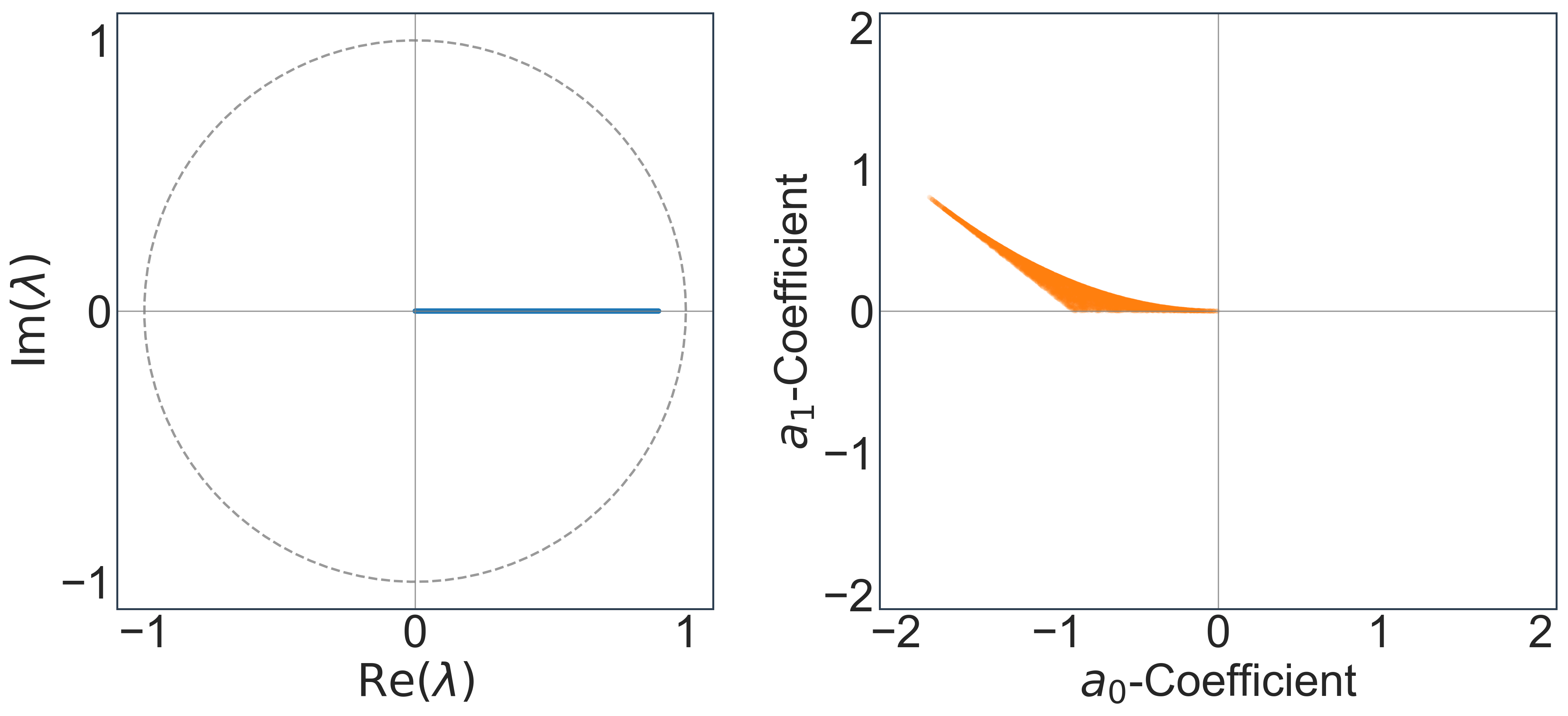
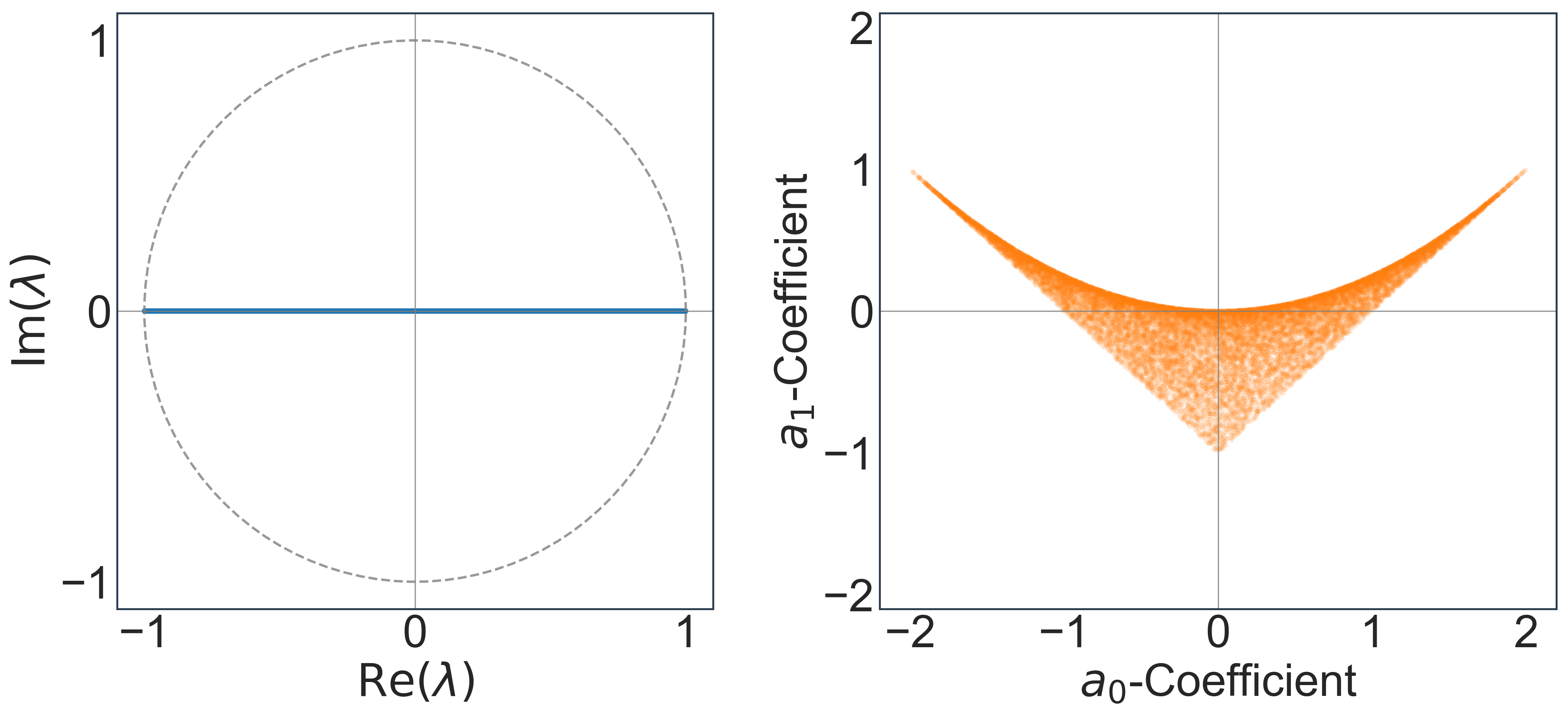
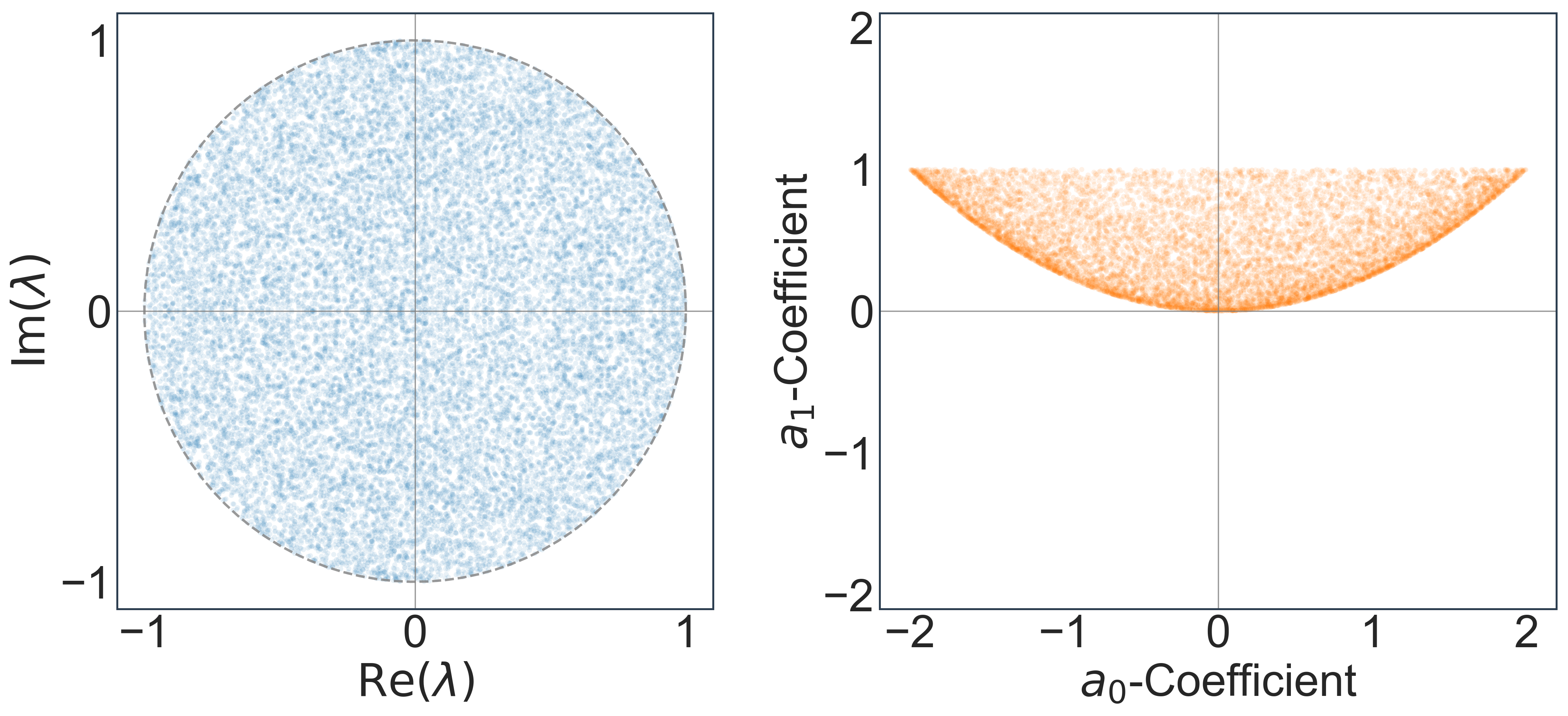
where represents a base prior density defined on or some subset thereof. Choices for reflect different assumptions or prior information about system behavior. Figure 1 illustrates several options for defining priors on eigenvalues within the unit disk (), which we discuss below.
Restricted region prior
Uniform real eigenvalue prior
A simple reference prior is to restrict eigenvalues to be real, . With a uniform base distribution , the stability constraint confines support to the real hypercube . Figure 1(b) shows samples on the real segment .
Polar coordinate prior
For complex eigenvalues (, ), priors can use polar coordinates. Non-informative choices might assume uniformity in area (e.g., ) and angle ( for the upper half-plane), as visualized in Figure 1(c).
Implied prior from uniform coefficients
Alternatively, a uniform prior can be placed on the characteristic polynomial coefficients within their stability region (e.g., the stability triangle for ). This induces a specific non-uniform mixture distribution on the eigenvalues, as depicted in Figure 1(d) and detailed for in Lemma 4.3.
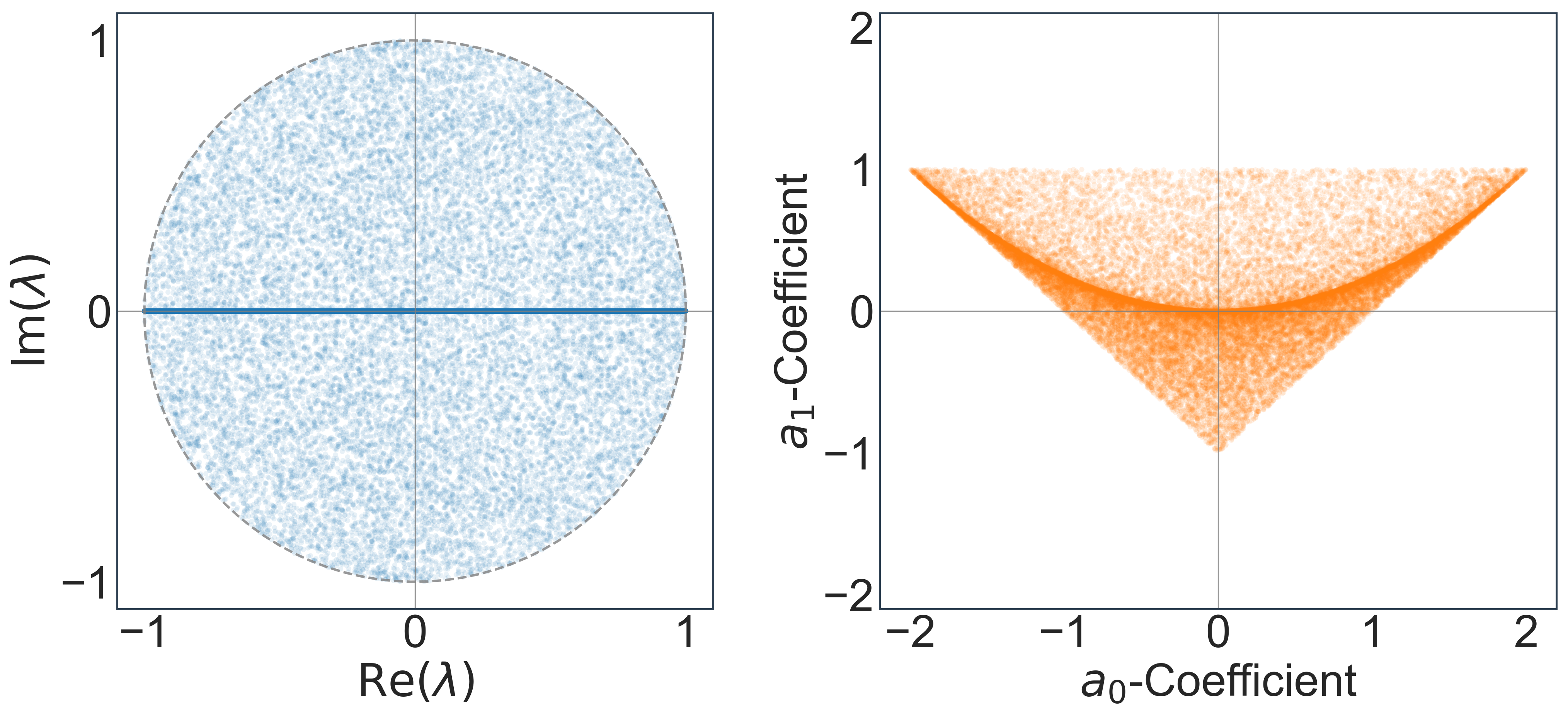
Lemma 4.3 (Implied eigenvalue density from uniform stable 2D systems).
Assume a uniform prior distribution over the coefficients corresponding to stable real LTI systems (i.e., uniform within the stability triangle defined by and ). The implied marginal probability density for a single eigenvalue is the mixture:
| (18) |
The proof is provided in D.10. This indicates a 2:1 preference for real eigenvalues over complex conjugate pairs when sampling uniformly from stable coefficients. The resulting density is uniform over for real eigenvalues and uniform over the upper (or lower) half of the open unit disk for complex eigenvalues. Figure 1(d) visualizes samples from this implied distribution.
The tendency for priors over stable real systems (whether defined on eigenvalues or implied by coefficient priors) to involve mixtures of real and complex eigenvalues, as explicitly derived in Lemma 4.3, is a general characteristic, formalized below.
Corollary 4.4 (Mixture distribution for eigenvalues of a stable system).
For any dimension , the eigenvalue spectrum of a stable real matrix comprises real eigenvalues in and complex conjugate pairs within the open unit disk, where the number of real eigenvalues, , satisfies with being an even number. Consequently, priors over the eigenvalues of stable real systems can be expressed as mixtures over the possible values of . The marginal density of a single eigenvalue can be written as:
| (19) |
where is the prior probability mass on having real roots; is the conditional density for a real eigenvalue given , supported on ; and is the conditional density for a complex eigenvalue given , supported on the open unit disk excluding the real line.
The proof is provided in D.11. This decomposition allows considerable flexibility in prior modeling through the specification of the base densities , , and the mixture weights . Even though for we have an explicit analytical result for the mixture weights, in higher dimensions their direct calculation becomes intractable. Such a calculation would rely on stability criteria, such as the Schur–Cohn test for determining whether all roots of the system’s characteristic polynomial lie within the unit disk, which are computationally infeasible for large . Consequently, estimating the weights via Monte Carlo simulation becomes the main approach.
Comparison with priors on matrix entries
Previous work in Bayesian system identification placed independent priors (e.g., ) on the entries of a full matrix [12]. Such entry-wise priors lack a clear connection to system-level behavior like stability or damping, making it difficult to encode meaningful prior knowledge. While one could try to use any of the eigenvalue priors discussed above while performing inference in the standard parameterization (i.e., over full matrices ), doing so would require evaluating the complex many-to-one mapping from to , which has an intractable Jacobian, and resolving its general non-invertibility. See further discussion in Remark D.8.
Placing priors directly on the coefficients of a canonical form is mathematically simpler, but still lacks the direct interpretability of eigenvalue priors. Therefore, defining a prior on eigenvalues and (via Proposition 4.2) transforming this distribution to a prior on the canonical coefficients represents an effective strategy. Note also that the the number of coefficients is exactly the same as the number of eigenvalues, such that and its Jacobian determinant are almost surely well defined (for the eigenvalue priors discussed above). This approach thus combines the intuitive control over system dynamics offered by eigenvalues with the computational benefits of working with a unique, identifiable canonical parameterization.
Remark 4.5 (Non-distinct eigenvalues).
A critical consideration arises when eigenvalues are not distinct. The map from eigenvalues to coefficients becomes singular at such points. While this degeneracy occurs only on a lower-dimensional subspace (typically assigned zero probability by continuous priors), it still has numerical implications. Eigenvalues that are very close cause the inverse Jacobian term to become extremely large. This numerical instability presents a practical hurdle for MCMC samplers exploring the parameter space near such degeneracies. Robust implementations may require numerical regularization, potentially facing sampling inefficiencies when the Jacobian becomes ill-conditioned, or necessitate alternative prior specifications (e.g., defining a prior directly on the canonical coefficients and enforcing stability through separate checks).
4.2 Priors over parameters ( and noise covariances)
While the prior on the state dynamics matrix (often specified via its eigenvalues ) demands careful consideration due to its strong influence on system behavior, priors on the remaining parameters are typically chosen based on simpler, standard considerations, often aiming for relative non-informativeness or some degree of regularization. For the SISO controller canonical form, parameters in , and consist of the numerator coefficients in the vector and the direct feed-through term . Common choices involve independent zero-mean Gaussian priors on these coefficients, e.g., and . The prior variances () can be fixed or assigned hyperpriors.
Priors for covariance matrices like and can be set directly, often using an inverse-Wishart distribution. For greater flexibility, the matrix can be parameterized via its Cholesky factor, , allowing for separate priors on its elements. Typically, zero-mean Gaussian priors are used for the off-diagonal elements, while distributions with positive support, such as half-Cauchy or Gamma, are used for the strictly positive diagonal elements. A key special case is when the covariance matrix is assumed to be diagonal. In this scenario, its Cholesky factor is also diagonal, and its entries directly correspond to the standard deviations of the noise terms. Therefore, placing a half-Cauchy prior on the diagonal elements of is equivalent to placing a prior directly on the standard deviations [1].
5 Posterior asymptotics: Bernstein–von Mises theorem
Understanding the asymptotic behavior of the posterior distribution is fundamental in Bayesian inference, providing insights into the efficiency of Bayes estimates and uncertainty calibration [13]. Here, we show that employing an identifiable canonical parameterization is essential for the validity of Bernstein–von Mises (BvM) results and the associated Gaussian posterior approximations, in the context of LTI system identification.
The BvM theorem is a cornerstone result [45] that establishes conditions under which the Bayesian posterior distribution converges to a Gaussian distribution centered at an efficient point estimate as the amount of data grows. This asymptotic normality links Bayesian inference to frequentist concepts and justifies Gaussian approximations for uncertainty quantification in large-sample regimes. Central to this theorem is the Fisher information matrix (FIM), which quantifies the information about the parameters contained in the data via the likelihood function, defining the precision of the limiting Gaussian posterior [45].
Definition 5.1 (Fisher information matrix).
Consider the likelihood function for parameters . Assume standard regularity conditions hold, ensuring differentiability of the log-likelihood with respect to and allowing interchange of differentiation and integration with respect to the data . The Fisher information matrix (FIM) at based on data up to time is:
Note that in our setting, the FIM is also a function of the known input or excitation . quantifies the expected curvature of the log-likelihood function at , representing the information provided about the parameter by an experiment with inputs yielding data . The definition above holds for both , i.e., estimation of full-dimensional LTI system matrices and for , i.e., estimation of the reduced parameters of a canonical form.
We now discuss the conditions under which a Bernstein-von Mises (BvM) theorem holds for Bayesian LTI system identification. For simplicity, our analysis focuses on the inference of the LTI dynamics matrices rather than the noise covariances. Crucially, our result requires that inference be performed using the canonical parameterization, (Definition 3.1), and that the dimension of the model class used for inference is consistent with the minimal dimension of the data-generating system.
Assumption 2 (Consistent state dimension).
The minimal state dimension of the data-generating system, denoted , equals the state dimension of the models described by .
Estimating the minimal state dimension itself from the data alone is considered an outer-loop problem, beyond the scope of the core inference task addressed here. Next, we require that the inputs be “sufficiently rich” to excite relevant aspects of the dynamics.
Definition 5.2 (Persistence of excitation).
A sequence of scalar inputs is persistently exciting of order if the limiting sample autocovariance matrix exists and is positive definite:
Under these conditions, and when performing inference with the canonical parameterization , we can prove a BvM. We state this theorem somewhat informally below; a more precise statement is given in Appendix C.
Theorem 5.3 (Bernstein–von Mises for LTI systems).
Let be the sequence of outputs generated by a SISO LTI system with true canonical parameters , given an input sequence that is persistently exciting of order . Assume the noise covariances are known, so that the -dimensional parameter vector contains only the canonical representation of the system dynamics matrices and, further, satisfies 2. Let denote the posterior distribution over this canonical parameterization. Under suitable regularity conditions on the likelihood (4) and the prior , the posterior distribution converges in total variation to a Gaussian distribution as , as follows:
| (20) |
where is a -consistent estimator (e.g., the MLE or MAP), is the posterior probability measure, and denotes the probability under a Gaussian distribution of a set . is the asymptotic Fisher information matrix per observation at the true parameter value, defined as , with being the FIM for observations. Convergence is in probability under the data-generating distribution , which has density .
In contrast with the preceding result, suppose we perform inference in the standard parameterization of the LTI system. Then, even if 2 is satisfied and the inputs are persistently exciting of order , the BvM fails to hold.
Theorem 5.4 (BvM failure in standard parameterizations).
BvM failure for the standard parameterization stems from a singular Fisher information matrix. This singularity occurs because is not identifiable; the posterior consequently fails to concentrate on a single point. Rather, it concentrates on the manifold of parameters related by similarity transformations. Employing an identifiable canonical parameterization is therefore essential to satisfy the conditions of Theorem 5.3. The canonical form provides local identifiability, while Gaussian noise and a persistently exciting input ensure likelihood regularity and a positive definite asymptotic FIM. For a detailed proof and discussion, see Appendix C.
Violating 2 has distinct implications depending on the direction of the mismatch. Overestimating the minimal state dimension—i.e., inferring a canonical model with —results in a singular Fisher information matrix, as redundant directions in parameter space are unidentifiable. Conversely, underestimating the minimal state dimension, i.e., setting , leads to model misspecification, rendering the parameter estimates inconsistent and violating key conditions required for a Bernstein–von Mises theorem to hold.
Fisher information matrix in canonical forms
The FIM is calculated by accumulating output sensitivities with respect to the canonical parameters; it can computed efficiently using recursive formulas. Detailed derivations, including explicit expressions for the FIM of the controller and observer forms (Proposition C.4) and extensions for systems with process noise via Kalman filter sensitivities (Proposition C.6), are provided in Appendix C. For finite-data scenarios, we also introduce an alternative metric for posterior geometry, the expected posterior curvature, in Section C.1.
6 Numerical experiments
This section presents numerical experiments designed to validate the theoretical advantages and evaluate the practical performance of Bayesian inference for LTI systems using canonical forms compared to using the standard, non-identifiable parameterization . We structure this section as follows: Section 6.2 details the common experimental setup, including system generation, noise specifications, algorithmic implementations, and parameter estimation methods. Section 6.3 analyzes the impact of canonical forms on posterior geometry and interpretability. Section 6.4 compares the computational efficiency and MCMC sampling performance between the canonical and standard approaches. Section 6.5 evaluates the accuracy of parameter estimates and QoIs, examining the influence of prior specifications, particularly in low-data regimes. Finally, Section 6.6 investigates asymptotic convergence properties related to the BvM theorem and assesses the computational scalability of the canonical form method with increasing system dimension.
6.1 Summary of key findings
The experiments detailed in the subsequent subsections demonstrate the following key advantages of using our proposed identifiable canonical forms for Bayesian LTI system identification:
-
(i)
Canonical forms yield well-behaved, typically unimodal posterior distributions suitable for reliable inference and interpretation, whereas standard forms result in complex, multimodal posteriors due to non-identifiability (Section 6.3, Figure 2, Figure 3), Figure 5 left panel).
-
(ii)
Inference using canonical forms exhibits higher computational efficiency, achieving higher effective sample size per second (ESS/s) compared to standard forms (Section 6.4, Figure 4).
-
(iii)
Bayesian inference with canonical forms provides accurate recovery of QoIs and outperforms baseline system identification methods such as the Ho–Kalman algorithm [31] (also called the eigensystem realization algorithm [28], particularly in low-data or noisy scenarios (Section 6.5, Figure 5 right panel, Figure 6, and Figure 7 left panel).
-
(iv)
While all tested priors lead to convergence with sufficient data, informative priors enhance accuracy significantly in data-limited regimes, and stability-enforcing priors provide robustness (Section 6.5, Figure 7).
-
(v)
Empirical results confirm asymptotic consistency and convergence of the canonical posterior towards the Gaussian distribution predicted by the BvM theorem, validating use of the FIM for uncertainty analysis (Section 6.6, Figure 8).
-
(vi)
Bayesian system identification in the canonical form demonstrates significantly better computational scalability with increasing system dimension compared to inference in the standard parameterization (Appendix A, Figure 9).
-
(vii)
MCMC samplers exploring the canonical parameter space demonstrate better mixing compared to standard parameter space samplers (Section 6.4, Figure 9 panel (d)).
6.2 Experimental setup and implementation
We use simulated data generated from known ground truth LTI systems. We set the feedthrough matrix in all experiments, as its inclusion does not significantly alter the relative performance comparison between parameterizations. We focus on stable LTI systems (), representing the most common practical scenario.
System generation methodology
Unless otherwise stated (e.g., for scalability tests in Section 6.6), a diverse random set of stable systems is generated as follows:
-
1.
Stable system matrix : We draw from a prior distribution over the space of stable matrices, designed based on eigenvalue distributions like the uniform polar prior discussed in Section 4.
-
2.
Input and output matrices : We independently draw each entry of and from a standard normal distribution, .
Ensuring controllability and observability
While random generation usually produces controllable and observable systems, numerical near-degeneracies can occur. To mitigate this, we compute the controllability Gramian and observability Gramian (convergent for stable ). Following [2], we assess conditioning by examining the eigenvalue spectra . We reject systems where the dominant eigenvalue accounts for more than 99% of the total energy (trace), i.e., if for either or . This filtering ensures that our test systems are robustly controllable and observable in practice. In real-world settings, this choice relates to the outer-loop problem of choosing a sufficient state space dimension .
Input and noise specifications
Persistently exciting inputs are generated as i.i.d. standard Gaussian random variables, . Process noise and measurement noise are independent zero-mean Gaussian sequences, with diagonal covariances and . The noise standard deviations and are either fixed per experiment or assigned normal priors if treated as unknown parameters.
Priors
Default prior distributions for model parameters are specified as follows; any deviations for particular experiments will be detailed in their respective subsections. For parameters in the standard state-space form , all coefficients are assigned independent standard normal priors. For parameters in canonical forms , the state dynamics matrix is assigned a uniform stable prior (as discussed in Lemma 4.3). Coefficients in the input matrix and output matrix are assigned independent standard normal priors.
Algorithmic implementation
Posterior distributions are sampled using several state-of-the-art tools, especially NUTS [18] via BlackJAX [6] and JAX [25] for automatic differentiation of the log-posterior. The log-likelihood is computed using a Kalman filter; a deterministic implementation is used for . NUTS step size and mass matrix are tuned during warm-up via window adaptation as introduced in Stan’s manual [38]. A small nugget () ensures covariance stability in the Kalman filter. We generate four chains, each with a sample trajectory of steps and a warm-up period (with window adaptation) of steps. Convergence is monitored using effective sample size (ESS) and the Gelman–Rubin statistic .
Parameter estimation
The posterior samples allow for the estimation of any quantity of interest that is a function of the model parameters. We consider two main point estimates. The first is the posterior mean estimate (PME), which is the empirical expectation of the quantity over the posterior distribution:
| (21) |
Note that setting to be the identity function recovers the PME of the parameters themselves. The second is a plug-in estimate, such as one based on the maximum a posteriori (MAP) parameter value:
| (22) |
It is important to note that for a general nonlinear function , the posterior mean estimate is not equivalent to the plug-in estimate that uses the posterior mean of the parameters, i.e., .
6.3 Posterior geometry and interpretability
We find that the LTI parameterization choice fundamentally shapes the posterior landscape. Canonical forms induce well-behaved posteriors, as illustrated for a T=400 experiment in Figure 2. Figure 2(a) shows the pair plot for canonical parameters, revealing a unimodal, approximately Gaussian distribution amenable to MCMC exploration and interpretation. The identifiable structure allows direct derivation of interpretable quantities, such as the posterior distribution of the dominant eigenvalues shown in Figure 2(b), offering clear insights into system stability and dynamics.
(a) Canonical Parameter Space ()

(b) Dominant Eigenvalue Distribution
In stark contrast, the standard parameterization suffers from complex posterior geometries due to non-identifiability. Figure 3(a) visualizes the posterior for the same system; strong correlations and distinct modes (corresponding to different choices of state basis ) are clearly visible, arising directly from the state-basis equivalence symmetry (Theorem 3.3). This multimodal structure hinders efficient MCMC sampling and complicates the interpretation of parameter estimates and uncertainties compared to the structure observed for the posterior of the canonical .
The distribution over the standard parameters is intrinsically linked to the canonical posterior via similarity transformations . Formally constructing by averaging over all such transformations is ill-posed due to the non-compactness of and the lack of a suitable uniform measure. To visualize the geometric structure induced by these equivalences without performing this ill-defined averaging, Figure 3(b) employs a pushforward restricted to the compact orthogonal subgroup , which possesses a unique uniform Haar measure. This visualization is generated by taking samples from the canonical posterior, drawing random orthogonal matrices uniformly from (achieved by applying the QR decomposition to matrices with i.i.d. standard Gaussian entries), applying the corresponding similarity transformation to obtain samples in the standard parameter space, and then plotting the resulting empirical distribution.
The distribution shown in Figure 3(b) reveals the intricate, non-elliptical geometry and strong parameter correlations introduced even by this restricted set of orthogonal transformations. This structure contrasts with the typically unimodal geometry of the canonical posterior itself shown in Figure 2(a). The potential ill-definition of the standard posterior is resolved by the specific choice of priors on .
(a) Standard Parameter Space ()
(b) Orthogonally Transformed Space
6.4 Computational efficiency and MCMC performance
The posterior geometry induced by canonical forms translates directly into improvements in MCMC sampling efficiency and overall performance compared to standard parameterizations.
We first quantify this efficiency gain across a range of conditions. Inference was performed using both canonical and standard forms on 20 randomly generated, well-conditioned LTI systems (2D state space, following the generation procedure in Section 6.2) with process noise and measurement noise . Data trajectories of lengths ranging from 50 to 1250 were used.
Figure 4 displays the effective sample size per second, averaged across all parameters and systems, for both parameterizations. The results demonstrate the efficiency of the canonical form. This efficiency gap tends to widen as increases, highlighting the computational advantage conferred by the identifiable, reduced-dimension canonical parameterization.
Beyond the aggregate ESS/s metric, the quality of MCMC exploration is enhanced. Trace plots, such as those shown later in Figure 9(d) for an 8D system, reveal better mixing and faster convergence for canonical parameters , while chains for standard parameters can exhibit slower mixing and jumps between distinct modes corresponding to equivalent system representations, further hindering efficient posterior exploration.
Even though we obtain a higher sampling efficiency compared to the standard parametrization, there can be still efficiency differences within the model class parameterizations via canonical forms, depending on the degree of identifiability of the system. We assess the sampling efficiency of canonical parameterizations by comparing performance on an “easy” LTI system, constructed to have well-balanced controllability and observability Gramians (see Appendix F), versus a “hard” system, specifically generated to have ill-conditioned Gramians (we sampled a system such that the dominant eigenvalue ratio is higher than ). Figure 5 presents results distributed over 15 noise realizations of the “easy” and “hard” system. Figure 5(a) shows that the canonical form for the “easy” system maintains higher ESS/s than for the “hard” system. Figure 5(b) assesses estimation accuracy for the canonical form parameters on both systems, plotting the mean squared error (MSE) between the posterior mean estimate and the true parameters , alongside the MSE for a baseline Ho–Kalman estimate (HKE) (transformed to canonical coordinates for comparison). This demonstrates the robustness of the canonical Bayesian approach across varying system conditioning levels.
(Left) ESS/second Comparison
(Right) Estimation Accuracy (MSE)
Collectively, these results establish the computational and MCMC performance advantages realized by adopting the proposed identifiable canonical forms for Bayesian LTI system identification.
We have also conducted experiments to compare the time-wise scaling of both standard and canonical forms with system dimension (see Appendix A), where we observe that Bayesian system identification performed over the canonical parameterization exhibits notably improved computational scalability with increasing system dimension when compared to inference using the standard parameterization. Furthermore, using a specific example, we highlight the distinct mixing behavior of the parameters under each form, as detailed in the Appendix A.
6.5 Recovering quantities of interest
Beyond computational aspects, we evaluate the accuracy of the resulting estimates and the role of prior information, particularly in data-limited scenarios.
Accuracy of point estimates and predictions
We assess the ability of each parameterization to recover the system’s behavior by examining inferred observed trajectories, and comparing estimates over a fixed 2D ground truth LTI system simulated with process noise and measurement noise .
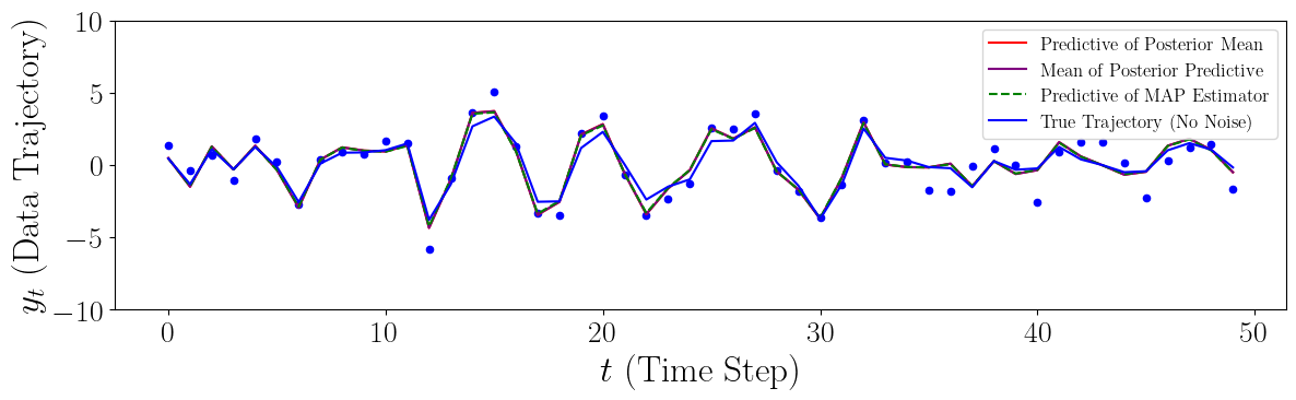
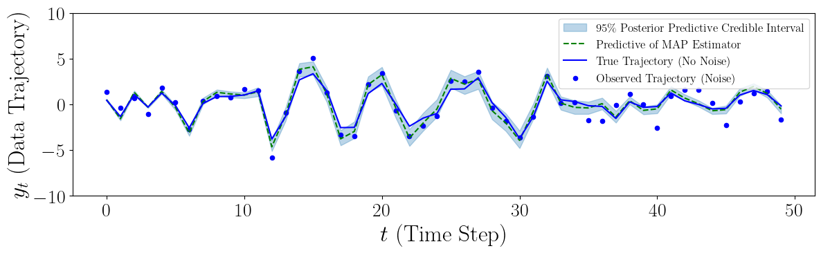
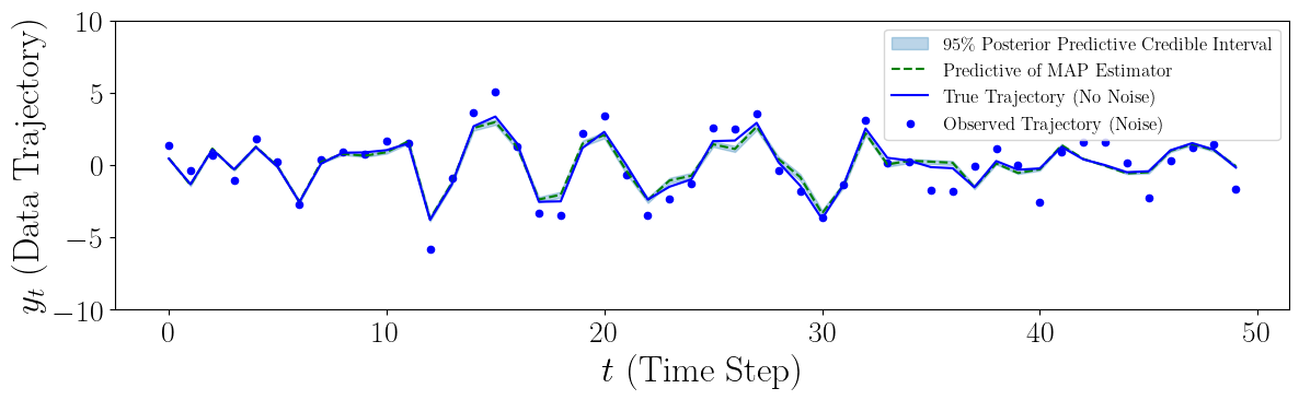
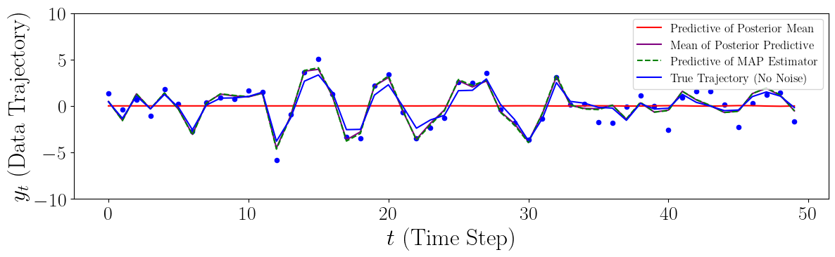
Figure 6 presents these comparisons. With sufficient data (), the MAP estimates derived from both the canonical (, Figure 6(b)) and standard (, Figure 6(e)) posteriors successfully track the true observed trajectory. This indicates that, given enough information, optimization can find a representative point within the correct equivalence class regardless of the parameterization’s identifiability issues.
However, differences emerge with limited data (), especially when considering the PME. While the MAP estimates for both forms ( Figure 6(a), Figure 6(d)) still capture the general trend reasonably well despite noise-induced fluctuations, the PME behaves distinctly. Derived from unimodal canonical posterior, (Figure 6(c)) provides a meaningful average parameter estimate that effectively smooths the observed trajectory. Conversely, the PME from the standard posterior, (Figure 6(f)), performs poorly, yielding an unrepresentative, nearly constant trajectory. This failure stems directly from the non-identifiability of : the posterior possesses multiple modes corresponding to the many observationally equivalent parameter sets (Theorem 3.3). Due partly to lower sampling efficiency (Section 6.4) and the MCMC chain potentially exploring or jumping between these distinct modes, the PME averages over structurally different system representations. This average, , consequently often lies in a region of low posterior probability between modes and does not correspond to any single valid system realization, thus failing to produce accurate predictions.
This result critically underscores the advantage of the canonical form: its enforced identifiability leads to a unimodal posterior where the PME serves as a robust and interpretable summary statistic for the system parameters.
(a) Canonical, , MAP
(b) Canonical, , MAP
(c) Canonical, , PME
(d) Standard, , MAP
(e) Standard, , MAP
(f) Standard, , PME
Prior sensitivity analysis
The influence of prior information is particularly pronounced in low-data regimes. To investigate this, we perform a Bayes risk analysis illustrated in Figure 7. We generated 30 ground truth systems by sampling eigenvalues from the restricted region prior as defined in Section 4.1.1 and applying random orthogonal transformations. Data trajectories up to steps were simulated with fixed measurement noise () and two levels of process noise: none (, top row) and moderate (, bottom row). Bayesian inference was performed using the canonical form under three different prior assumptions: the restricted region prior, which we will call the “Informative Prior”; and two “Weakly Informative Priors,” the stable polar prior and uniform prior as defined in Section 4.1.1. For an additional baseline comparison, we use the HKE [31], which provides a non-Bayesian point estimate (distinct from a prior-based approach) for baseline comparison.
Accuracy is assessed using the median (over 30 systems) Frobenius norm error of the Hankel matrix derived from the PME (, Figure 7(a, c)) and the median over the system’s MSE of the canonical parameters (, Figure 7(b, d)), plotted against on log-log scales.
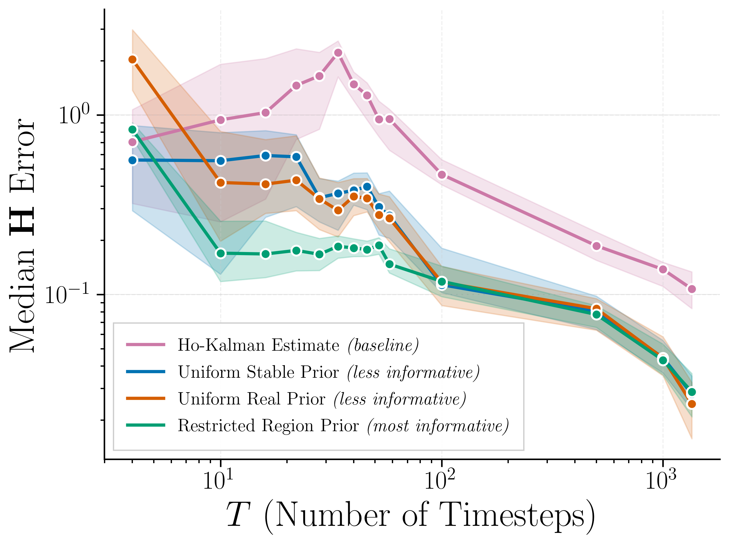
(a) Hankel error,
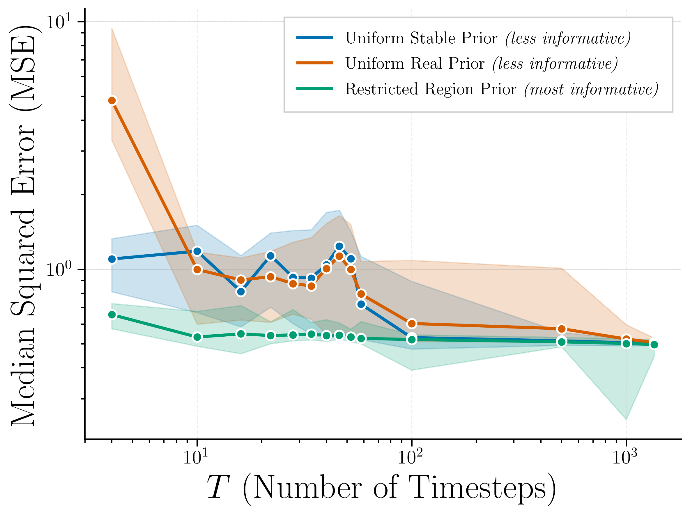
(b) MSE,
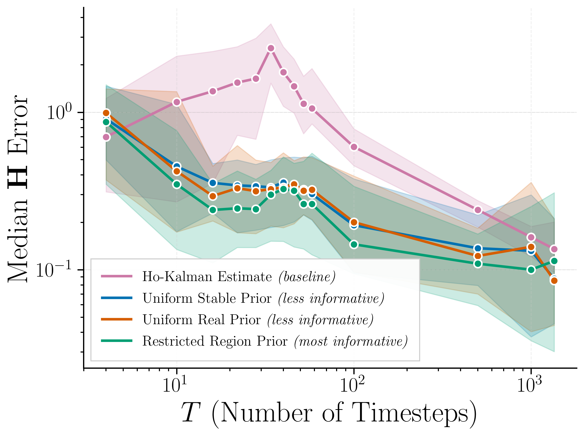
(c) Hankel error,
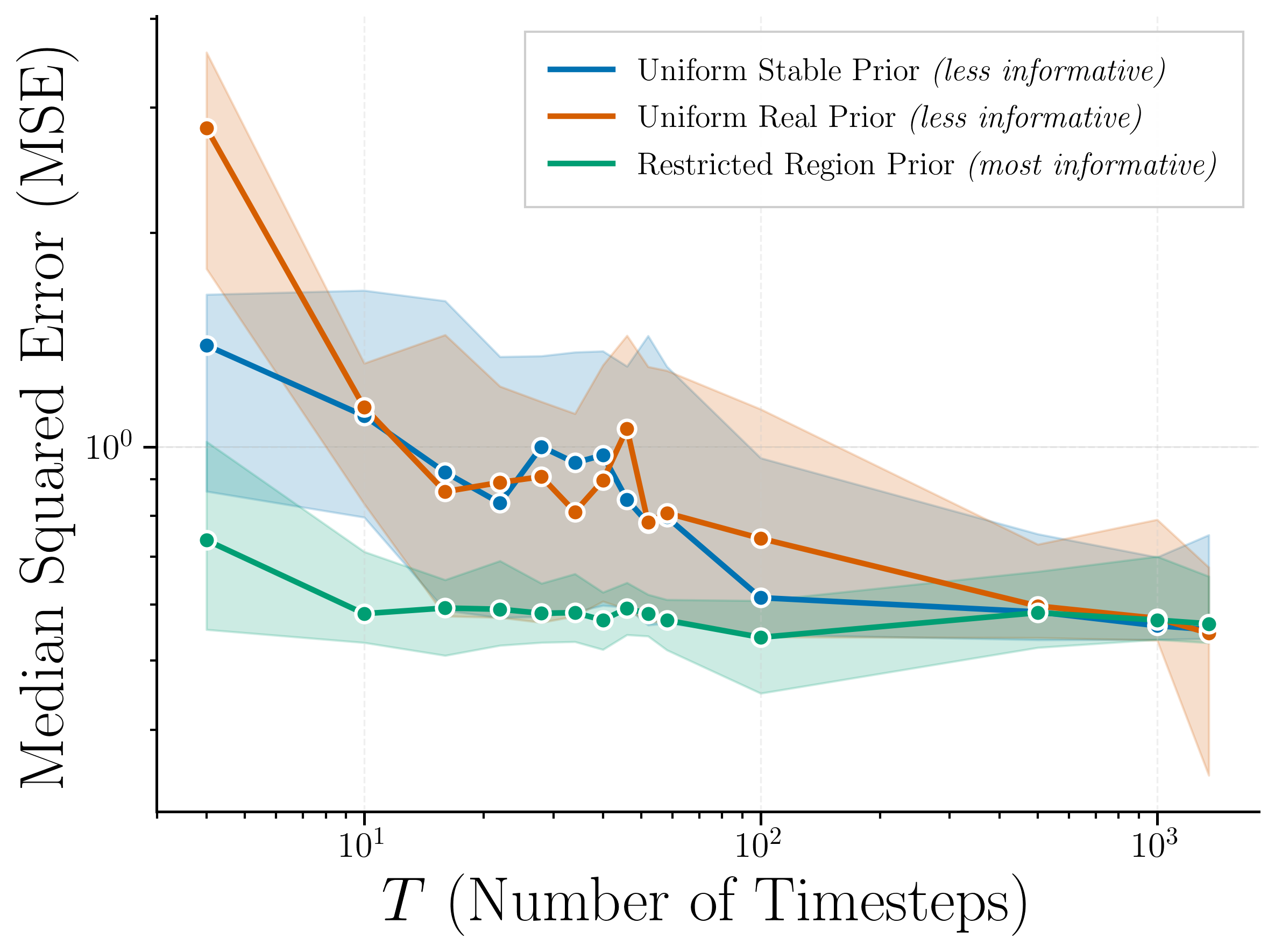
(d) MSE,
As expected, Figure 7 shows that for small , the informative prior yields the lowest error, significantly outperforming less informative priors and the baseline, highlighting the value of accurate prior information when data is scarce. The parameter MSE (panels b, d) consistently shows the benefit of the informative prior across both noise levels. However, the Hankel error (panels a, c), which relates more directly to the input-output impulse response, shows a more nuanced picture. In the presence of process noise (, panel c), the advantage of the informative prior in terms of Hankel error diminishes at very low , becoming comparable to the HKE or the weakly informative prior. This suggests that while the informative prior leads to better average parameter estimates, process noise can obscure the initial impulse response, making direct estimation like Ho-Kalman estimate competitive for predicting short-term input-output behavior with very limited, noisy data. Nonetheless, as increases, the likelihood information dominates, all Bayesian methods converge, and they consistently outperform the baseline, demonstrating the robustness of the Bayesian canonical inference framework, especially with stability-enforcing priors.
6.6 Asymptotic convergence and scalability
We empirically validate the consistency of parameter estimates and the convergence of the posterior distribution towards the Gaussian shape predicted by the Bernstein-von Mises theorem (see Theorem 5.3) for identifiable canonical forms. This experiment uses 15 randomly generated ground truth systems. For each system, data is simulated with zero process noise () and fixed measurement noise over increasing trajectory lengths . From this simulated data, we determine the MAP estimate of the canonical parameters, denoted as .
A key aspect of BvM is the role of the FIM. We compare two FIM calculations, both evaluated at the MAP estimate for each ground truth system: (1) , computed using the recursive formulas derived in Proposition C.4. These formulas are exact for the case considered here. (2) , an approximation of the expected FIM. This is obtained by first generating independent noisy trajectory realizations using the ground truth parameters. A single MAP estimate, , is computed from one of these realizations (which we designate as the reference realization). Then, the observed FIM is computed for each of the realizations by applying automatic differentiation (AD) to the log-likelihood (using JAX), with each observed FIM being evaluated at this single derived from the reference realization. Finally, these observed FIMs are averaged. This AD-based approach provides an efficient way to estimate the expected FIM and readily extends to scenarios with non-zero process noise where analytical formulas become more complex (see Appendix C).
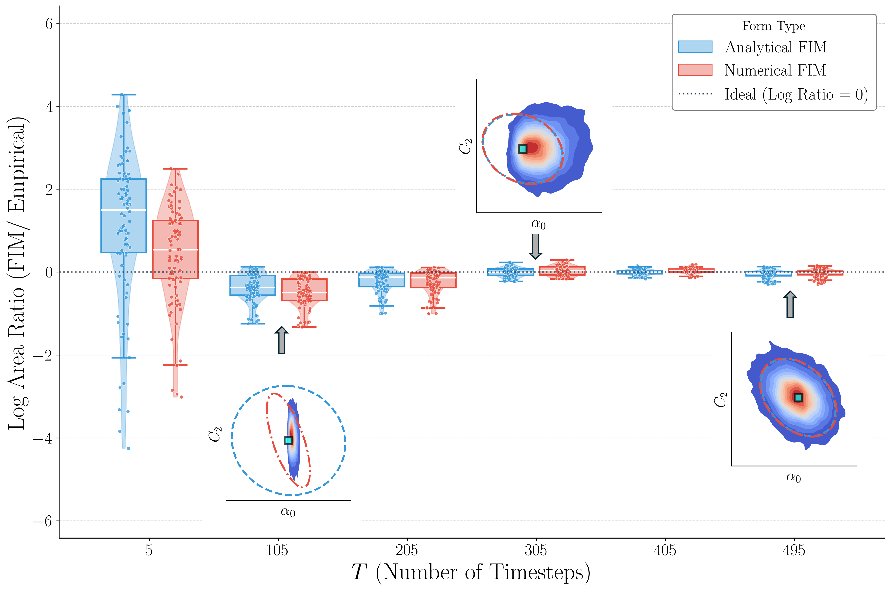
Figure 8 illustrates the agreement between these two FIM calculations. The main plot shows boxplots of the logarithm of the ratio of the volumes of the confidence ellipsoids derived from and . As increases, this log ratio converges towards zero, indicating that the numerical approximation accurately captures the information content described by the analytical FIM. The insets visualize the posterior density contours from MCMC samples overlaid with the confidence ellipsoid derived from an FIM (e.g., ) for selected parameters (e.g., ) at different trajectory lengths . These clearly show the posterior distribution concentrating and becoming increasingly elliptical (Gaussian-like), aligning well with the FIM-based prediction. This empirically validates the BvM theorem’s assertion of asymptotic normality for the canonical parameterization. Although not explicitly plotted, analyses confirmed that the MSE of the posterior mean decreases appropriately with , and the empirical coverage of confidence intervals approaches nominal levels, further supporting consistency.
7 Conclusions and future work
We have presented an efficient Bayesian framework for identifying linear time-invariant dynamical systems from single-trajectory data, leveraging identifiable state-space canonical forms. We have demonstrated both theoretically and empirically the significant advantages of our canonical approach over inference based on standard parameterizations.
Summary of contributions
Our core contribution is the integration of canonical state-space representations with principled Bayesian inference to resolve the intrinsic non-identifiability of linear dynamical systems. We prove that inference on these identifiable canonical forms yields the same posterior distributions for invariant quantities of interest as inference in standard but non-identifiable parameterizations (Proposition 3.8). We also show that this framework facilitates meaningful prior specification (e.g., directly on eigenvalues controlling dynamical properties). It also yields posterior concentration around a consistent parameter estimate and justifies Gaussian posterior approximations, as described by a Bernstein–von Mises theorem (Theorem 5.3); this is not the case for standard parameterizations. Numerical experiments show that our canonical approach consistently provides superior computational efficiency compared to standard parameterizations (Section 6).
Limitations
Though it is much more computationally efficient than inference on (Section 6.4), our MCMC approach inherently carries a higher computational burden than non-Bayesian point estimation methods for system identification (e.g., subspace ID or Ho–Kalman estimates [46, 31]); this gap reflects the cost of full Bayesian uncertainty quantification, as well as the improved performance of posterior mean estimates (as observed in our numerical experiments). We also note that computational performance may be sensitive to the specific canonical form chosen, notably for MIMO systems. Another key consideration is our assumption of a known state dimension . Determining from data, in the present Bayesian setting, is a problem of Bayesian model selection. It is solved by comparing marginal likelihoods across dimensions—a principled but computationally intensive approach, which may be especially relevant if the “practical” system order is lower than the minimal one, given finite and limited data.
Extensions and future work
To further contextualize our Bayesian state-space approach to system identification, we comment briefly on the alternative possibility of a Bayesian approach that uses transfer function representations, e.g., parameterizing models directly via poles and zeros. We suggest that practical difficulties would arise with such a representation. For instance, posterior exploration using sampling methods such as MCMC may suffer from numerical instability or poor convergence properties when proposals fall near pole locations of the true (data-generating) system, which dictate system dynamics and stability boundaries.
Fully instantiating Bayesian inference in canonical representations for MIMO systems presents several further challenges. The intricate structure of MIMO systems complicates structural identifiability analysis, demanding more sophisticated prior specification methods that make sense of internal parameter structure. Inference schemes may then need to be tailored to specific structural indices (Remark 3.2). Despite the non-uniqueness of canonical forms in the MIMO setting, the foundational results of this paper can still hold by making a choice and committing to one specific form. But it is natural to then consider “hybrid” inference methods that exploit multiple, equivalent canonical forms; these might improve sampling efficiency near controllability or observability boundaries.
Another important extension, as mentioned above, is to move beyond fixed model orders and infer the state dimension itself, e.g., using Bayesian model selection methods or some approximate information criterion. From a theoretical standpoint, a key challenge is to quantify finite-sample performance by deriving rigorous non-asymptotic bounds on posterior convergence with increasing data, moving beyond the typical Bernstein–von Mises guarantees. To tackle very high-dimensional systems, addressing scalability is essential; we suggest exploring variational inference methods or stochastic gradient MCMC tailored to state-space structures. Finally, extending structure-informed Bayesian techniques to nonlinear systems, with a similar decomposition of the model class into identifiable and non-identifiable features, represents a considerably more challenging but highly promising direction.
References
- [1] I. Alvarez, J. Niemi, and M. Simpson, Bayesian inference for a covariance matrix, 2014, https://arxiv.org/abs/1408.4050.
- [2] A. C. Antoulas, Approximation of Large-Scale Dynamical Systems, vol. 6 of Advances in Design and Control, Society for Industrial and Applied Mathematics, Philadelphia, PA, 2005, https://doi.org/10.1137/1.9780898718713, https://epubs.siam.org/doi/10.1137/1.9780898718713.
- [3] A. Y. Aravkin, J. V. Burke, A. Chiuso, and G. Pillonetto, Sparse/robust estimation and Kalman smoothing with nonsmooth prior distributions, IEEE Transactions on Automatic Control, 57 (2012), pp. 2596–2609.
- [4] A. Bakshi, A. Liu, A. Moitra, and M. Yau, A new approach to learning linear dynamical systems, 2023, https://arxiv.org/abs/2301.09519, https://arxiv.org/abs/2301.09519.
- [5] E. J. Barbeau, Polynomials, Problem Books in Mathematics, Springer Science & Business Media, New York, 2003.
- [6] A. Cabezas, A. Corenflos, J. Lao, R. Louf, A. Carnec, K. Chaudhari, R. Cohn-Gordon, J. Coullon, W. Deng, S. Duffield, G. Durán-Martín, M. Elantkowski, D. Foreman-Mackey, M. Gregori, C. Iguaran, R. Kumar, M. Lysy, K. Murphy, J. C. Orduz, K. Patel, X. Wang, and R. Zinkov, Blackjax: Composable bayesian inference in jax, 2024, https://arxiv.org/abs/2402.10797, https://arxiv.org/abs/2402.10797.
- [7] M. C. Campi and L. Ljung, Perspectives on system identification, in The 17th International Symposium on Mathematical Theory of Networks and Systems (MTNS2006), 2006, pp. 19–45.
- [8] J. E. Cavanaugh and R. H. Shumway, On computing the expected fisher information matrix for state–space model parameters, Statistics & Probability Letters, 26 (1996), pp. 347–355, https://doi.org/10.1016/0167-7152(95)00031-3, https://doi.org/10.1016/0167-7152(95)00031-3.
- [9] C.-T. Chen, Linear System Theory and Design, Oxford University Press, Inc., USA, 3rd ed., 1998.
- [10] N. Chopin, P. E. Jacob, and O. Papaspiliopoulos, Smc2: an efficient algorithm for sequential analysis of state space models, 2013, https://doi.org/https://doi.org/10.1111/j.1467-9868.2012.01046.x, https://rss.onlinelibrary.wiley.com/doi/abs/10.1111/j.1467-9868.2012.01046.x, https://arxiv.org/abs/https://rss.onlinelibrary.wiley.com/doi/pdf/10.1111/j.1467-9868.2012.01046.x.
- [11] B. P. M. Duarte, M. d. R. Reis, J. A. Costa, B. Herz, L. Pibouleau, G. Trystram, and J. Antony, Optimal experimental design for linear time invariant state–space models, tech. report, 2021.
- [12] N. Galioto and A. A. Gorodetsky, Bayesian system id: optimal management of parameter, model, and measurement uncertainty, Nonlinear Dynamics, 102 (2020), p. 241–267, https://doi.org/10.1007/s11071-020-05925-8, http://dx.doi.org/10.1007/s11071-020-05925-8.
- [13] A. Gelman, J. B. Carlin, H. S. Stern, D. B. Dunson, A. Vehtari, and D. B. Rubin, Bayesian Data Analysis, CRC Press, Boca Raton, Florida, third ed., 2013.
- [14] M. Gevers, Identification for control: From the early achievements to the revival of experiments, European Journal of Control, 11 (2005), pp. 335–352.
- [15] M. Hardt, T. Ma, and B. Recht, Gradient descent learns linear dynamical systems, Journal of Machine Learning Research, 19 (2018), pp. 1–44, http://jmlr.org/papers/v19/16-465.html.
- [16] S. M. Hirsh, D. A. Barajas-Solano, and J. N. Kutz, Sparsifying priors for bayesian uncertainty quantification in model discovery, Royal Society Open Science, 9 (2022), p. 211823, https://doi.org/10.1098/rsos.211823, https://doi.org/10.1098/rsos.211823.
- [17] H. Hjalmarsson, From experiments to models: A sparse journey through system identification, Automatica, 41 (2005), pp. 757–793.
- [18] M. D. Hoffman and A. Gelman, The no-u-turn sampler: Adaptively setting path lengths in hamiltonian monte carlo, 2011, https://arxiv.org/abs/1111.4246, https://arxiv.org/abs/1111.4246.
- [19] Y. Hu, A. Wierman, and G. Qu, On the sample complexity of stabilizing lti systems on a single trajectory, 2022, https://arxiv.org/abs/2202.07187, https://arxiv.org/abs/2202.07187.
- [20] A. Juditsky, H. Hjalmarsson, A. Benveniste, B. Delyon, L. Ljung, J. Sjöberg, and Q. Zhang, Nonparametric identification of linear systems, Automatica, 31 (1995), pp. 1725–1750.
- [21] T. Kailath, Linear Systems, Prentice-Hall, 1980.
- [22] R. E. Kálmán, Mathematical description of linear dynamical systems, Journal of the Society for Industrial and Applied Mathematics, Series A: Control, 1 (1963), pp. 152–192, https://doi.org/10.1137/0301010, https://doi.org/10.1137/0301010.
- [23] N. Kantas, A. Doucet, S. S. Singh, J. Maciejowski, and N. Chopin, On particle methods for parameter estimation in state-space models, Statistical Science, 30 (2015), https://doi.org/10.1214/14-sts511, http://dx.doi.org/10.1214/14-STS511.
- [24] A. Katsevich, Improved dimension dependence in the bernstein von mises theorem via a new laplace approximation bound, 2024, https://arxiv.org/abs/2308.06899, https://arxiv.org/abs/2308.06899.
- [25] M. Lin, Automatic functional differentiation in jax, 2024, https://arxiv.org/abs/2311.18727, https://arxiv.org/abs/2311.18727.
- [26] L. Ljung, System Identification: Theory for the User, Prentice Hall information and system sciences series, Prentice Hall PTR, 1999, https://books.google.com/books?id=nHFoQgAACAAJ.
- [27] L. Massai and G. Ferrari-Trecate, Free parametrization of -bounded state space models, 2025, https://arxiv.org/abs/2503.23818.
- [28] R. Minster, A. K. Saibaba, J. Kar, and A. Chakrabortty, Efficient algorithms for eigensystem realization using randomized SVD, SIAM Journal on Scientific Computing, 43 (2021), pp. A3395–A3421, https://doi.org/10.1137/20M1327616, https://doi.org/10.1137/20M1327616.
- [29] N. Morse and R. Sacksteder, Statistical Isomorphism, The Annals of Mathematical Statistics, 37 (1966), pp. 203 – 214, https://doi.org/10.1214/aoms/1177699610, https://doi.org/10.1214/aoms/1177699610.
- [30] B. Ninness and S. r. Henriksen, Bayesian system identification via Markov chain Monte Carlo techniques, Automatica, 46 (2010), pp. 40–51, https://doi.org/10.1016/j.automatica.2009.10.015, https://doi.org/10.1016/j.automatica.2009.10.015.
- [31] S. Oymak and N. Ozay, Non-asymptotic identification of lti systems from a single trajectory, 2019, https://arxiv.org/abs/1806.05722, https://arxiv.org/abs/1806.05722.
- [32] V. Peterka, Bayesian system identification, Automatica, 17 (1981), pp. 41–53, https://doi.org/10.1016/0005-1098(81)90024-1, https://doi.org/10.1016/0005-1098(81)90024-1.
- [33] G. Pillonetto and L. Ljung, Full bayesian identification of linear dynamic systems using stable kernels, Proceedings of the National Academy of Sciences, 120 (2023), p. e2218197120, https://doi.org/10.1073/pnas.2218197120, https://doi.org/10.1073/pnas.2218197120.
- [34] R. Pintelon and J. Schoukens, System Identification: A Frequency Domain Approach, John Wiley & Sons, 2nd ed., 2012.
- [35] S. J. Qin, An overview of subspace identification, Computers & Chemical Engineering, 30 (2006), pp. 1502–1513.
- [36] C. R. Rojas, J. S. Welsh, G. C. Goodwin, and A. Feuer, Input design for mimo subspace identification: Optimal magnitude and power allocation, Automatica, 44 (2008), pp. 2792–2796.
- [37] T. Sarkar, A. Rakhlin, and M. A. Dahleh, Nonparametric finite time lti system identification, 2020, https://arxiv.org/abs/1902.01848, https://arxiv.org/abs/1902.01848.
- [38] Stan Development Team, Stan Reference Manual, 2025, https://mc-stan.org/docs/2_23/reference-manual/index.html. Version 2.23.
- [39] F. Stilgenbauer, M. Zorzi, A. Magnani, E. Napoli, G. Palumbo, G. Van der Plas, and G. G. Gielen, Symbolic state-space extraction for faster and more accurate mixed-signal behavioral modeling, in 2024 Design, Automation & Test in Europe Conference & Exhibition (DATE), IEEE, 2024, pp. 1–6, https://doi.org/10.23919/DATE5872DATE58725.2024.10510932.
- [40] A. Svensson, A. Solin, S. Särkkä, and T. B. Schön, Computationally efficient bayesian learning of gaussian process state space models, in Proceedings of the 19th International Conference on Artificial Intelligence and Statistics (AISTATS), vol. 51 of Proceedings of Machine Learning Research, 2016, pp. 213–221, https://proceedings.mlr.press/v51/svensson16.html.
- [41] S. Särkkä, Bayesian Filtering and Smoothing, vol. 3 of Institute of Mathematical Statistics Textbooks, Cambridge University Press, 2013, https://doi.org/10.1017/CBO9781139344203, https://doi.org/10.1017/CBO9781139344203.
- [42] M. E. Tipping, Sparse Bayesian learning and the Relevance Vector Machine, Journal of Machine Learning Research, 1 (2001), pp. 211–244.
- [43] I. Urteaga and P. M. Djurić, Sequential Estimation of Hidden ARMA Processes by Particle Filtering—Part I, IEEE Transactions on Signal Processing, 65 (2017), pp. 482–493, https://doi.org/10.1109/TSP.2016.2598309.
- [44] I. Urteaga and P. M. Djurić, Sequential Estimation of Hidden ARMA Processes by Particle Filtering—Part II, IEEE Transactions on Signal Processing, 65 (2017), pp. 494–504, https://doi.org/10.1109/TSP.2016.2598324.
- [45] A. W. Van der Vaart, Asymptotic Statistics, vol. 3 of Cambridge Series in Statistical and Probabilistic Mathematics, Cambridge University Press, 1998.
- [46] P. Van Overschee and B. De Moor, Subspace Identification for Linear Systems: Theory - Implementation - Applications, Springer Science & Business Media, 1996.
- [47] B. Wahlberg and L. Ljung, On the consistency of the least-squares method in system identification, Automatica, 22 (1986), pp. 547–557.
- [48] J. Wang, K. Liu, Q. Jin, Z. Yang, J. Zhang, and B. Ran, A review on digital twin technology for lithium-ion battery management, Energy and AI, 14 (2023), p. 100295, https://doi.org/10.1016/j.egyai.2023.100295.
- [49] W. X. Zheng and Y. Ohta, Parameter estimation of mimo systems from noisy input-output measurements, Automatica, 40 (2004), pp. 471–477.
Appendix A Scalability with dimension
Our final experiment investigates how computational performance scales with system dimension . We generate test systems with ranging from 2 to 10 using a specific procedure designed to yield balanced controllability and observability properties, crucial for fair comparison across dimensions (see Appendix F.
We compare the computation time for inference using standard and canonical forms on these balanced systems for fixed trajectory lengths and . Figure 9 presents the timing results (normalized per evaluation where appropriate). Figure 9(a) and Figure 9(b) show the time required for posterior and gradient evaluations, respectively. The cost for the standard form increases markedly faster with dimension than for the canonical form. While the gradient computation for the canonical form might have slightly higher overhead at the lowest dimension () due to its specific structure, its superior scaling becomes evident quickly. This advantage arises because standard state-space operations (like the Kalman filter) inherently involve dense matrix calculations scaling polynomially with (e.g., ), whereas the often sparse structure of canonical forms allows for more efficient implementations. Figure 9(c) confirms this trend for the total inference time, demonstrating substantial computational savings with the canonical approach, especially for .
Beyond computation time, MCMC sampling efficiency also benefits from the canonical form in higher dimensions. Figure 9(d) shows diagnostics for an system (T=500). The trace plot for a canonical parameter () exhibits good mixing and exploration of a concentrated posterior, reflected in the unimodal histogram centered near the true value (albeit with a slight offset, potentially due to noise or minor model misspecification). In contrast, the trace plot for a corresponding standard parameter () shows poorer mixing, and its histogram is significantly more dispersed. This difference in sampling behavior is typical across parameters and underscores the advantage of the well-behaved canonical posterior landscape for efficient MCMC exploration in higher dimensions. We also note a subtle point: our inference assumes diagonal noise covariances , whereas the balancing transformation applied to the original system could induce off-diagonal terms in the true noise covariances of the balanced system. This slight model misspecification might contribute to small biases observed in estimates like that in Figure 9(d). Currently, our inference assumes a simplified noise model, estimating a single variance parameter proportional to a standard normal distribution for both process and measurement noise. While a more accurate approach would involve learning the full Cholesky factors of the covariance matrices and , we have observed that the associated computational cost is substantial, and a diagonal covariance assumption provides a valid simplification even under model misspecification, suggesting inference of diagonal matrices for and as a practical recommendation.
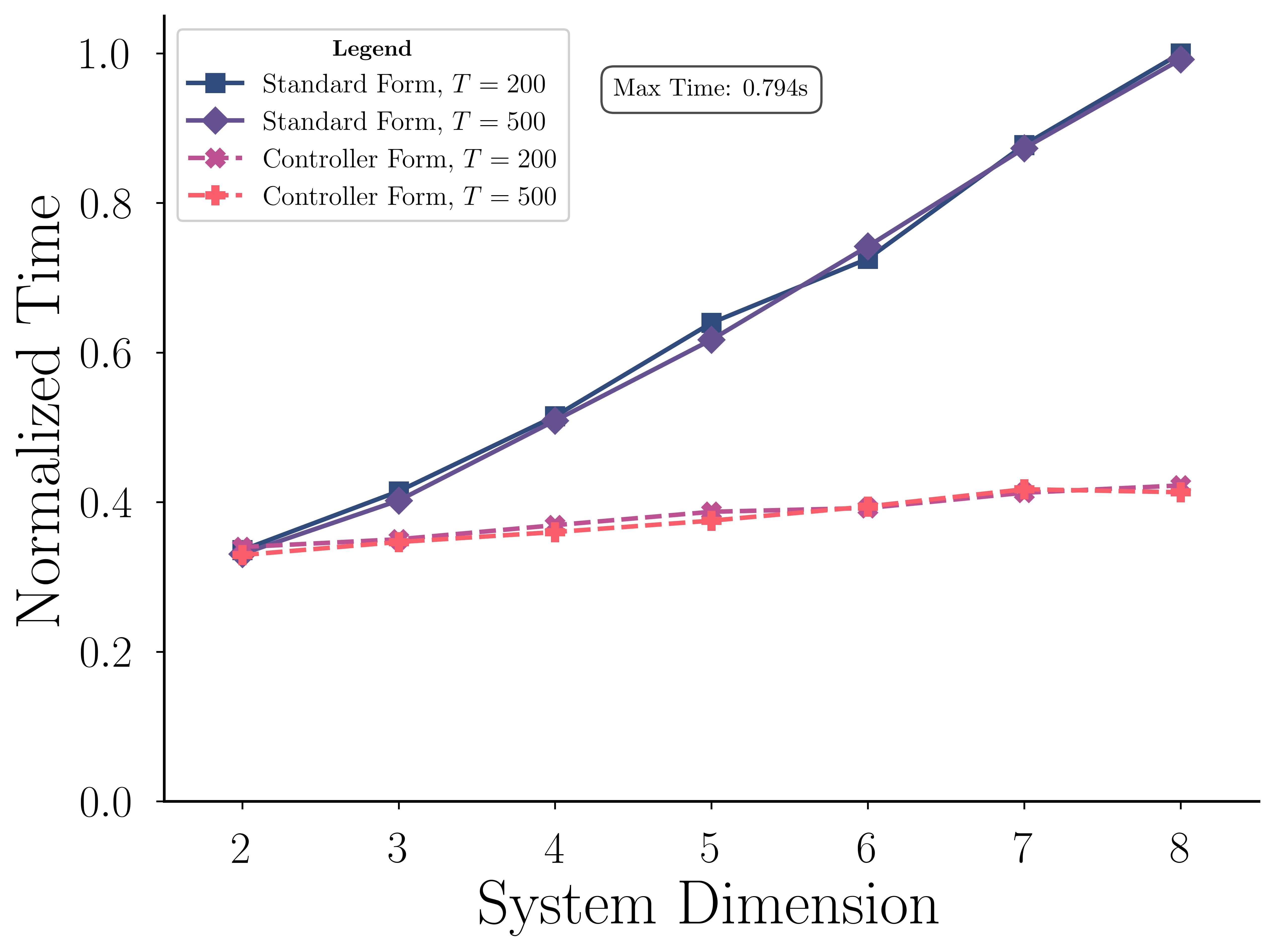
(a) Posterior Eval Time
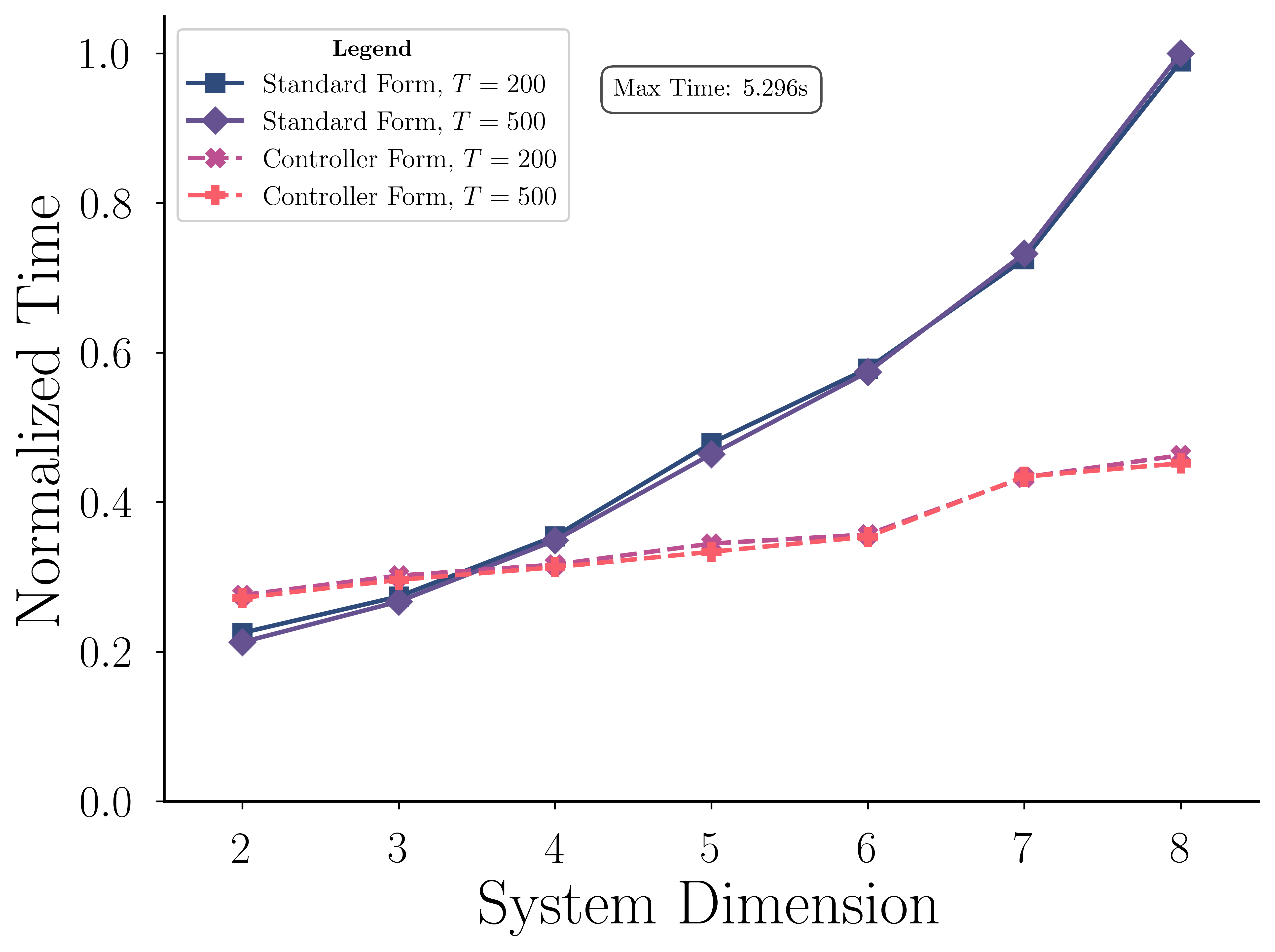
(b) Gradient Eval Time
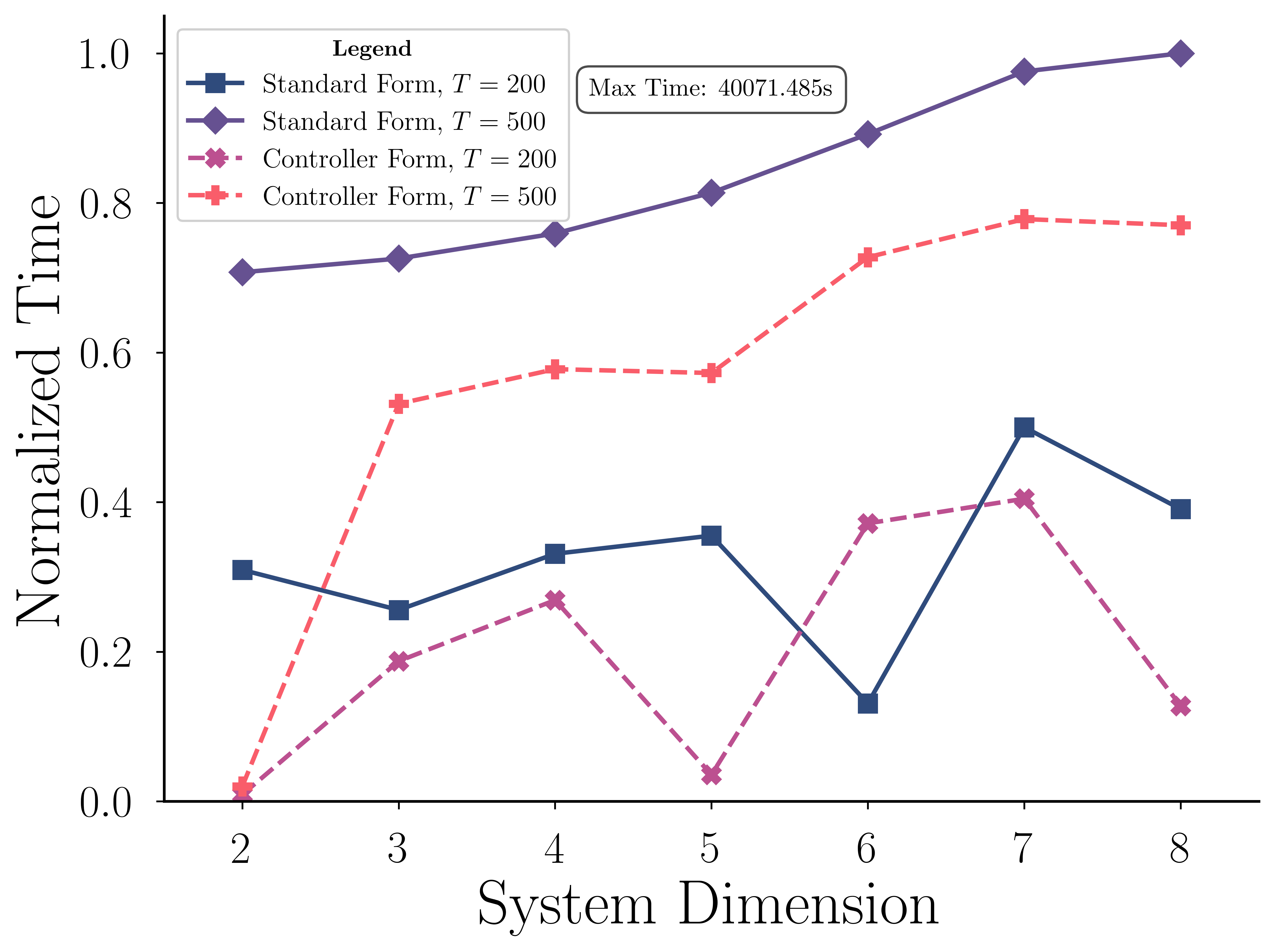
(c) Total Inference Time
(d) MCMC diagnostics (, )
Appendix B Likelihood decomposition
We are interested in the posterior , we define the prior , which we will discuss in detail in Section 4. We obtain:
| (23) |
Define probabilistic characterization of system behavior: The likelihood is given explicitly:
| (24) |
| (25) |
Under the assumption that both the process and emission noises are normal, we can obtain the likelihood for the state-update and the observation step, respectively:
| (26) | ||||
| (27) |
We follow the ideas by [41] and describe the procedure of likelihood recursion in the following theorem:
Theorem B.1 (Marginal likelihood recursion).
Let and denote the sequences of observations and inputs. Assume that the state-space model is given by (1) with an initial prior on , where the parameter set is . Then, under the assumption that both the process and observation noises are Gaussian, the marginal likelihood
can be computed recursively via the following three steps for :
-
1.
Prediction: Compute the predictive density
(28) -
2.
Update: Evaluate the one-step-ahead observation likelihood via
(29) -
3.
Marginalization: Update the filtering distribution for the state by
(30)
By iterating these steps from (with ) to , one obtains the marginal likelihood
as well as the sequence of filtering distributions for each time step.
Appendix C Fisher information and BvM
We follow [45] and state the BvM in full generality here:
Theorem C.1 (Bernstein-von Mises theorem for LTI systems).
Consider a discrete-time LTI system with the state-space representation (1). Let and denote the observed outputs and inputs up to time . Let be the parameter vector, where is an open subset of . Suppose that:
-
1.
Regularity and identifiability: The true parameter is an interior point of , and the model is structurally identifiable in the canonical form. Moreover, the likelihood is smooth in , and the system is both controllable and observable at .
-
2.
Local asymptotic normality (LAN): The sequence of dynamical system experiments satisfies the LAN property at ; that is, for a suitable sequence of estimators (e.g., the maximum likelihood estimator) with converging in distribution, the log-likelihood admits the expansion
(31) where converges in distribution to , and is the Fisher Information Matrix for the LTI system.
-
3.
Persistence of excitation: The input sequence persistently excites, as defined in
-
4.
Prior regularity: The prior density is positive and continuous in a neighborhood of .
Then, if denotes the posterior distribution of given the observations and inputs, we have that
| (32) |
as . Equivalently, the posterior distribution of the rescaled parameter converges in total variation to the multivariate normal distribution , where .
Proof C.2 (Proof of Theorem C.1(Theorem 5.3)).
We begin by proving the applicability of BvM for the canonical form. Let denote the parameter vector in canonical form, where is the minimal number of parameters required to characterize an -dimensional LTI system with inputs and outputs. The minimal canonical form uses exactly parameters, which is the minimal number required to uniquely characterize the input-output behavior of an -dimensional LTI system. Each parameter in appears exactly once in a specific position in the system matrices. For any two distinct minimal canonical parameter vectors , the corresponding transfer functions differ: see [9]). The log-likelihood function for this Gaussian system has the quadratic form. The Fisher Information Matrix (FIM) is therefore:
| (33) |
Following the argument above we conclude that the FIM is non-singular as for canonical forms. Persistent excitation implies that converges to a positive definite matrix as , ensuring that all state variables are influenced by the inputs. These two properties together ensure that the limit of the normalized FIM:
| (34) |
is positive definite for canonical parameterizations, which contain exactly the minimal number of parameters needed to characterize the input-output behavior.
Furthermore, the log-likelihood ratio for canonical parameters satisfies the Local Asymptotic Normality condition, given that the innovation sequence consists of independent Gaussian random variables with zero mean and covariance , the Central Limit Theorem ensures that , where . Thus, all conditions of the Bernstein-von Mises theorem are satisfied for canonical parameterizations, and the posterior distribution converges in total variation to a normal distribution.
Proof C.3 (Proof of Theorem 5.4).
The BvM theorem fails for standard form parameterization , where all entries of matrices , , , and are treated as free parameters. The fundamental issue is the existence of equivalence classes under similarity transformations. This creates equivalence classes in parameter space:
| (35) |
Each equivalence class forms an -dimensional manifold in parameter space (where is the state dimension), since has free elements. For any tangent vector to the manifold at :
| (36) |
This holds because moving along direction doesn’t change the system’s input-output behavior, hence doesn’t affect the likelihood. Consequently:
| (37) |
making the FIM necessarily singular for standard parameterization. Due to this singularity, the posterior distribution cannot converge to a non-degenerate normal distribution in all directions of the parameter space.
The geometric interpretation is that the posterior distribution in standard form becomes concentrated on an -dimensional manifold rather than at a point, with its shape on this manifold determined by the prior distribution even in the asymptotic limit. This violates the core premise of the BvM theorem, which requires the posterior to converge to a normal distribution entirely determined by the data through the MLE and FIM.
Proposition C.4 (Fisher information for LTI systems in canonical forms).
Consider an LTI system with deterministic state dynamics given by (1), where is an i.i.d. sequence of Gaussian noise with for and . Assume that the system is in either the controller or observability canonical form. Let denote the vector of system parameters (which includes either the entries of or those of ; in the observer form the the derivative would be with respect to ). Then, the Fisher information matrix corresponding to the likelihood function is given by
| (38) |
where we have used the fact that . Moreover, the derivatives in (38) can be computed recursively via the product rule. In particular, for the parameters affecting the state matrix (which appear in the controller form) the recursion is
| (39) |
and for the parameters of (when is free, as in the controller form),
| (40) |
In the observer canonical form, since is fixed, the differentiation is carried out with respect to the parameters in the matrix, and analogous recursive formulas hold.
Proof C.5 (Proof of Proposition C.4).
The log-likelihood of the output sequence given the parameter vector is derived from the Gaussian noise assumption. For each time step , the observation is given by , where . The probability density function of a single observation is therefore . Since the noise samples are independent and identically distributed, the likelihood of the entire sequence is the product of the individual probabilities, . The log-likelihood function, , is then the sum of the individual log-likelihoods:
The Fisher Information Matrix is defined as the negative expectation of the Hessian of the log-likelihood function, i.e., . Let’s compute the first partial derivative of with respect to a generic parameter :
The second partial derivative with respect to is:
Taking the expectation, we note that . Thus, the second term vanishes. This leaves:
Since the state evolution is deterministic given the inputs and initial state, the derivative is non-random. Therefore, the expectation operator can be removed, and we can express the Fisher Information Matrix in vector form as stated in (38):
To derive the recursive formulas, we first express the state as a function of the initial state and the input sequence : . The output is . For a parameter in the state matrix , we differentiate with respect to . Using the product rule and the formula for the derivative of a matrix exponential, we get:
The derivative of the matrix power is . Substituting this into the expression for and then multiplying by yields the result in (39). For a parameter in the output matrix , the state does not depend on . The derivative is simpler:
which gives (40). The reasoning for the observer canonical form, with differentiation with respect to parameters in , follows an analogous procedure.
The derivation, including the case with process noise () requiring Kalman filter sensitivities, is discussed in the following proposition. We follow the derivation of [8] and adapt the equations to the canonical forms:
Proposition C.6 (Fisher information for LTI systems in canonical forms via Kalman filter).
Consider an LTI system represented in a canonical form:
| (41) |
with initial state , process noise , and measurement noise . Let the parameter vector consist of the variable entries in the system matrices. For the controller form the parameter vector is , where are the coefficients in the last row of and are the elements of . The matrix is assumed known. The observer form’s parameter vector contains the variable entries of and , while is fixed. The log-likelihood function, derived from the Kalman filter’s prediction error decomposition, is:
| (42) |
where is the dimension of the output , is the innovation, and is the innovation covariance. The Fisher Information Matrix (FIM) is given by:
| (43) |
where denotes the vectorization of the matrix . The derivatives and are computed by propagating the derivatives of the parameters through the Kalman filter equations, with the derivatives of fixed matrix entries being zero.
Proof C.7 (Proof of Proposition C.6).
The foundation of this proof is the prediction error decomposition provided by the Kalman filter. The likelihood of the full observation sequence can be factored as . For a linear Gaussian system, the Kalman filter establishes that each one-step-ahead conditional distribution is Gaussian:
where is the predicted state and is the predicted observation covariance. The log-likelihood of a single observation is:
Summing over all time steps gives the total log-likelihood as stated in the proposition. The Fisher Information Matrix is defined as . To compute this, we first find the score function . Differentiating with respect to a single parameter involves the chain rule and standard matrix derivative identities ( and ):
To find the -th entry of the Hessian, we differentiate again with respect to and take the negative expectation. The key statistical properties of the innovations are that they are zero-mean, , and are white, i.e., . Consequently, when taking the expectation of the Hessian, all terms that are linear in vanish. The remaining non-zero terms arise from products of derivatives. Specifically, we use . The resulting -th element of the FIM is:
The second term can be written using the Kronecker product () and vectorization (), yielding the compact matrix form presented in the proposition.
For a system in a canonical form, the derivatives , , and are sparse matrices containing only a ’1’ or ’-1’ at the position of the parameter , and zeros elsewhere. For instance, in controller form, if , then is zero everywhere except for a ’-1’ at position . If , then is zero everywhere except for a ’1’ at position . These sparse derivatives are propagated through the recursive derivative equations for the Kalman filter states () and predictions (), to compute the required gradients and at each time step. The initialization is handled by the derivatives of the initial state, and , which are typically assumed to be zero if the initial conditions are not functions of .
Proposition C.8 (Efficient FIM calculation for canonical forms via Kalman filter sensitivities).
Consider an LTI system in a canonical form with parameters . The Fisher Information Matrix (FIM) is given by:
| (44) |
The efficiency in this calculation stems from specializing the general derivative recursions to the sparse structure of the canonical form matrices. The required sensitivities are computed as follows:
1. Controller canonical form
Here, the parameter vector is . The derivatives and are sparse matrices (containing only one non-zero element). This simplifies the general derivative recursions significantly. For each parameter , we compute:
| (45) | ||||
| (46) | ||||
| (47) | ||||
| (48) |
These sensitivities are then used to compute the derivatives of the Kalman gain and the updated state and covariance, which are needed for the next time step’s recursion.
2. Observer canonical form
Here, the parameter vector is . The derivatives and are sparse. The efficient recursions become:
| (49) | ||||
| (50) | ||||
| (51) | ||||
| (52) |
Note that derivatives with respect to are zero as it is fixed in this form.
Proof C.9 (Proof of Proposition C.8).
The derivation provides a computational procedure. The FIM formula is standard for Gaussian models and is derived from the negative expectation of the Hessian of the log-likelihood. The efficiency comes from exploiting the structure of the canonical forms when computing the required derivatives.
The general sensitivity equations for the Kalman filter are obtained by direct differentiation of the filter’s time- and measurement-update equations. For any parameter , we have:
And similarly for the remaining filter quantities (). The matrix derivatives (e.g., ) are extremely sparse, typically containing only a single non-zero entry.
Controller form:
For a parameter , we have and is a matrix of zeros with a ’-1’ at position . For a parameter , we have and is a row vector of zeros with a ’1’ at position . Substituting these sparse matrices into the general sensitivity equations simplifies them to (45)-(48). For example, in (45), if , the term is zero, so the equation simplifies to . This sparsity propagates through the recursions, making the computation highly efficient as many terms become zero.
Observer form:
The logic is identical. Here, is fixed, so for all parameters. For , the derivative is sparse, and for , the derivative is sparse. Substituting these into the general equations yields the simplified set (49)-(52). For example, the term involving vanishes from the derivative of , leaving the much simpler (51).
This specialization avoids unnecessary matrix operations with zero matrices, providing a clear and efficient algorithm. At each time step , one runs the Kalman filter and, in parallel, the set of recursive derivative equations (where is the number of parameters), using the results to update the total FIM sum.
C.1 Expected posterior curvature
Distinct from the likelihood-based Fisher Information Matrix (FIM) , which depends solely on the likelihood and involves expectation over data , one can assess the posterior’s average concentration using the Expected Posterior Curvature matrix, . This metric captures the negative expected Hessian of the log-posterior (thus incorporating both likelihood and prior influence), averaged with respect to the posterior itself, offering a finite-sample perspective on uncertainty (see Definition C.10). While reflects the average posterior shape for finite data and the likelihood’s curvature, they are related—the Bernstein-von Mises theorem (Theorem 5.3) links the asymptotic posterior shape to the limiting FIM . However, they measure distinct aspects of information and curvature, especially for finite .
Definition C.10 (Expected posterior curvature matrix).
Consider the posterior distribution for parameters . Assume the log-posterior is twice differentiable with respect to (treated as a flattened vector of free parameters), and that the expectations below exist. The Expected Posterior Curvature Matrix is defined as the negative expectation of the Hessian of the log-posterior, where the expectation is taken with respect to the posterior distribution itself:
Equivalently, under regularity conditions:
quantifies the average concentration of the posterior distribution .
Appendix D Proofs of Section 1-5
Proof D.1 (Proof of Theorem 3.3).
Since and yield the same outputs for all possible input sequences , their internal states must be related by an invertible linear transformation. Minimality (both controllability and observability) guarantees the existence and uniqueness (up to an invertible scaling) of such a transformation.
Let and be the respective state trajectories of and . Define for some invertible . Substituting into the equations of ,
| (53) |
and multiplying by , we compare with the corresponding state-space equations of to conclude:
| (54) |
Moreover, since the output distributions of and match for all noise realizations and initial conditions, the covariance matrices must also transform appropriately. Specifically,
| (55) |
where remains invariant because the measurement output is not itself transformed (only the state is). Finally, minimality (both controllability and observability) ensures there are no other hidden degrees of freedom that could produce the same input-output distributions. In particular, one cannot introduce further transformations that decouple unobservable modes. Hence is unique up to non singular scaling factors that leave the system equations unchanged in any physically meaningful sense. Consequently, and are isomorphic under the similarity transformation given by , completing the proof.
Proof D.2 (Proof of Theorem 3.5).
Let
| (56) |
be the characteristic polynomial of . Define the auxiliary polynomials
| (57) |
with and (setting ). These polynomials satisfy
| (58) |
Next, define the vectors for . By the Cayley–Hamilton theorem, we have .
Because is controllable, the vectors form a basis of . Moreover, are related to this basis via the invertible transformation
| (59) |
Hence, is itself a basis. Defining , the polynomial relation implies
| (60) |
for . From this recursion, one directly obtains the canonical (companion) form of . Finally, since , we have .
Proof D.3 (Proof of Lemma 3.7).
Let the prior density on the standard space define a measure such that for any measurable set , its measure is . Using the canonical projection map , we define a pushforward measure, , on the canonical space . By definition, the measure of any set under is the measure of its pre-image, .
By the Radon–Nikodym theorem, since the measure is absolutely continuous with respect to the Lebesgue measure on , there exists a unique (up to a set of measure zero) density function such that the measure can be computed as an integral of this density: . This function is the induced prior density.
By equating the definition of the pushforward measure with its representation via the Radon–Nikodym derivative we uniquely set up the relation:
| (61) |
for any measurable set , where is the pre-image of .
Proposition D.4 (Invariance under similarity transformations).
Let and be parameterizations of two minimal LTI systems related by a similarity transformation such that , , , and . Then the following key system properties are identical for both parameterizations:
-
1.
The sequence of Markov parameters, for , and the feedthrough term, .
-
2.
The eigenvalue spectrum of the dynamics matrix, .
These properties imply that the Hankel matrices and transfer functions of the two systems are also identical.
Proof D.5 (Proof of Proposition D.4).
We begin by proving part (i). The Markov parameters transform under as:
Since both the Hankel matrix and transfer function are constructed entirely from Markov parameters:
their invariance follows directly from the invariance of . The eigenvalue invariance follows from:
Furthermore, computing eigenvalues from the companion matrix of a canonical form (e.g., (7)) offers computational advantages compared to general matrices. The computational advantage of using a canonical form for eigenvalue analysis is substantial. For a general matrix in a standard parameterization, the eigenvalues are found numerically using a direct eigensolver, such as the QR algorithm. The computational cost of this operation is floating-point operations.
In contrast, for a matrix in a canonical representation (e.g., the controller or observer form), the coefficients of its characteristic polynomial are directly available from its entries. The task is then reduced to finding the roots of this -th degree polynomial. Numerically solving for the roots using robust iterative methods (like the Jenkins-Traub algorithm) has a typical complexity of .
Proof D.6 (Proof of Proposition 3.8).
and are compact subsets of Euclidean space equipped with the Borel -algebra and Lebesgue measure. We write if there exists such that:
| (62) |
This relation partitions into equivalence classes . The measurability of this partition follows from the fact that the map is continuous. For each equivalence class , we select a unique canonical form representative . The mapping that assigns each standard form to its canonical form is explicitly constructable (e.g. for the controller form Theorem 3.5). Define the bounded general linear group:
| (63) |
For sufficiently large , and for any , there exists such that . This follows from the normalization properties of canonical forms. The set is compact in the Euclidean topology on , as it is the intersection of the closed set with the open set . It carries a well-defined Borel -algebra and can be equipped with a finite measure . For any transformation matrix :
| (64) |
as we have established in Theorem 3.3. As prior can vary within equivalence classes:
| (65) |
we need to carefully keep track of the differently distributed masses. By Bayes’ theorem, the posterior will also generally vary within the respective equivalence classes. For any canonical form , its preimage under is:
| (66) |
However, this parameterization is redundant. For minimal systems with distinct eigenvalues, the stabilizer is given by:
| (67) |
The equivalence class is thus precisely characterized as:
| (68) |
where denotes the equivalence class of in the quotient space. The quotient space carries a well-defined Borel -algebra and measure. Specifically, let be the Haar measure on , which exists and is unique up to a scaling factor because is a compact topological group.
The quotient measure on is defined for any measurable set in the quotient space as:
| (69) |
For any measurable set , we define the posterior probability as:
| (70) |
By the disintegration theorem, this integral can be broken down into integrals over individual fibers for each :
| (71) |
where is the conditional measure on the fiber .
The explicit form of the conditional measure can be expressed using the quotient space structure:
| (72) |
where is the Jacobian determinant of the parameterization map. Using Bayes’ theorem and the invariance of the likelihood:
| (73) |
For any , applying the conditional measure formula:
| (74) |
We define the induced prior on the canonical form as:
| (75) |
This defines a proper probability measure on that accounts for the variation of the prior density across the equivalence class corresponding to . For any measurable set in the space of system-level quantities, the set consists of entire equivalence classes. This follows from the invariance of under similarity transformations (see Proposition D.4). Therefore:
| (76) | ||||
This establishes the equivalence of pushforward posteriors for standard and canonical forms with an arbitrary prior distribution, not necessarily constant over equivalence classes.
Remark D.7 (Normal priors and canonical form).
While we cannot place normal priors directly on matrices B and C in the standard form parameterization while maintaining equivalence class invariance, we can achieve this by working in the canonical form.
By placing normal priors on B’ and C’ in the canonical form and then inducing a prior on standard form through the canonical mapping, invariance is automatically guaranteed. This works because all equivalent systems map to the same unique canonical form representative. Thus, two equivalent systems (related by similarity transformation) will have identical prior probability by construction, preserving the required invariance property.
This approach allows modelers to specify intuitive normal priors while maintaining mathematical rigor in the Bayesian inference process. In practice, this means we can perform inference directly in the canonical form with normal priors on B’ and C’, and simultaneously place invariant priors on eigenvalues of A’, yielding a theoretically sound and computationally efficient Bayesian framework.
Remark D.8 (Challenges in prior specification with standard parametrization).
Consider a discrete-time LTI system (1) of dimension . Consider the case, if we relax, that the priors are the same for the equivalence class, let us see that it still leads to several challenges. We examine how Gaussian priors on state-space matrices transform to canonical parameterizations and the resulting implications for Bayesian inference. A common approach places independent Gaussian priors , , on each matrix entry. While this specification appears intuitive, it introduces significant complications when considering system properties that are invariant to the choice of state-space realization.
For controllable pairs , there exists an invertible similarity transformation that yields the controller canonical form. The transformation matrix is constructed from coefficients of the characteristic polynomial of see Theorem 3.5:
The characteristic polynomial coefficients can be expressed using exterior algebra as:
| (77) |
where is the trace of the -th exterior power of , computable via the determinant formula:
| (78) |
This transformation is fundamentally nonlinear. For a simple matrix case, the characteristic polynomial demonstrates that while the trace term is linear in the entries of , the determinant term exhibits quadratic nonlinearity. To quantify how probability measures transform under this nonlinear mapping, we examine the Jacobian matrix. For our example, key entries include , , and , further illustrating the mixture of linear and nonlinear dependencies.
The transformed probability density follows , and as the inverse is dense, leads to increased computational cost. When considering eigenvalues instead of canonical form coefficients, additionally it introduces several complications. First, the transformation from matrix entries to eigenvalues involves solving polynomial equations, which is inherently nonlinear. Second, eigenvalues are unordered, leading to permutation invariance that creates multimodality in the transformed distribution.
Proof D.9 (Proof of Proposition 4.2).
Write
| (79) |
Using Vieta’s formula we identify the coefficients with the products and sums of eigenvalues. We can write the Jacobian as:
| (80) |
Using induction one can show, that the matrix is equivalent to the Vandermonde matrix, which has an explicit formula given by:
| (81) |
Proof D.10 (Proof of Lemma 4.3).
The characteristic polynomial of any 2×2 real matrix has the form . For a stable system whose eigenvalues lie within the unit disk, the coefficients must satisfy the Schur-Cohn stability conditions: and . These inequalities define a triangular region in the plane with total area 4 square units.
The discriminant determines the nature of the eigenvalues. The curve (a parabola given by ) divides into two subregions: where eigenvalues are real, and where eigenvalues are complex.
Computing the area of requires integrating over the region where within the stability constraints:
| (82) |
The area of is then .
Therefore, under a uniform distribution on in , the probability of real eigenvalues is , and the probability of complex eigenvalues is .
For purely imaginary eigenvalues, we require and , which corresponds to a line segment in with Lebesgue measure zero under the two-dimensional uniform distribution. To derive the specific density functions in each region, we apply the Jacobian transformation from the coefficient space to the eigenvalue space. For real eigenvalues the uniform density in transforms to a constant density on . For complex eigenvalues the uniform density in transforms to a constant density over the unit disk in the complex plane.
Proof D.11 (Proof of Corollary 4.4).
For a -dimensional real matrix, the characteristic polynomial has degree . Since eigenvalues of real matrices either occur as real values or complex conjugate pairs, the number of real eigenvalues must satisfy .
For a stable system, all eigenvalues must lie within the unit disk. Given real eigenvalues, the remaining eigenvalues form complex conjugate pairs.
Let be a probability mass function over admissible values of . Then the eigenvalue distribution can be expressed as a mixture:
| (83) | ||||
| (84) |
For , this recovers Lemma 4.3 with and .
Appendix E Canonical forms in LTI systems
In control theory, canonical forms provide standardized representations of linear time-invariant systems. Here we present all eight canonical forms divided into controllability and observability categories.
E.1 Multi input multi output systems (MIMO)
Definition E.1 (MIMO canonical structure example).
A possible canonical structure for MIMO systems ( or ) uses a block companion form for , often parameterized by structural indices like the observability index . For instance, with state dimension , one such identifiable structure is given by the matrices :
| (85) |
where is the identity matrix, () are scalar parameters defining the characteristic polynomial blocks, the matrices () contain free parameters representing the system’s numerator dynamics (Markov parameters), and the feedthrough matrix also consists of free parameters (unaffected by state basis transformations). The set of free parameters defining the system dynamics within this canonical form is explicitly:
This specific dynamic structure contains free parameters. Using the relationship , this count can be expressed as . The full canonical parameter set, , encompasses both these dynamic parameters and the parameters describing the noise statistics. Assuming Gaussian noise (1) as discussed in Section 3.1, the noise parameters consist of the unique elements of the lower (or upper) triangular Cholesky factors. Therefore, the complete set of parameters to be inferred is . The noise components and contribute an additional parameters to the total count in .
E.2 Controllability SISO canonical forms
.
(1) Controller form
(2) Dual controller form
(3) Observable-style controller
(4) Dual observable-style controller
E.3 Observability SISO canonical forms
.
(5) Observer Form
(6) Dual observer form
(7) Controller-style observer
(8) Dual controller-style observer
Appendix F Details on numerical experiments
Procedure for Generating Well-Conditioned LTI Systems
To generate stable, high-dimensional, and well-conditioned test systems for comparison, we employ a systematic procedure for a given state dimension . First, an initial discrete-time LTI system pair is defined to be stable and controllable by choosing the dynamics matrix to be diagonal, , with distinct eigenvalues linearly spaced on the real interval . The input matrix is set to a column vector of ones, , which guarantees the pair is controllable. Next, to normalize the system’s input-to-state mapping, we compute the controllability Gramian, , as the unique symmetric positive definite solution to the discrete-time algebraic Lyapunov equation . A state transformation matrix is then defined as the unique symmetric positive definite square root of this Gramian. Applying this similarity transformation yields a new system realization , where and , whose controllability Gramian is the identity matrix . Finally, to make the overall system nearly balanced, an output matrix is constructed such that its observability Gramian, , which solves , is as close to the identity matrix as possible. This is achieved using the ”uniform proportions method”, a heuristic wherein is constructed from the left eigenvectors of the system matrix . Specifically, given the eigendecomposition , the output matrix is set proportional to the sum of the rows of (which are the left eigenvectors), i.e., , where . This construction ensures that has a significant projection onto every system mode, making observability uniform across all states. The resulting system is thus stable, fully controllable, observable, and approximately balanced, making it an excellent benchmark for numerical methods.