Abstract

This study explores the field of modified inertia through a novel model involving maximal and minimal acceleration bounds. A principle of dynamics is developed within special relativity and has direct implications in astrophysics, especially for galaxy rotation curves. The presence of a minimal acceleration significantly reduces the amount of dark matter required to account for these curves. The model presented here is however conceptually different from fiduciary Modified Newtonian Dynamics (MOND). The modified inertia with the minimal acceleration bound closely matches with many observed galaxy rotation curves and the radial acceleration relation, showing a better agreement than MOND in the $10^{-10}$ m s^-2 regime. Additionally, the minimal acceleration is predicted to evolve with redshift.

Keywords : Dark matter; modified dynamics; galactic dynamics; quantum speed limit.

1 Introduction

With the emergence of the problem of rotation curves in galaxies [1, 2, 3, 4, 5], it was proposed that a new type of matter fills the Universe. This particular matter, supposed to reach up to five times the quantity of ordinary baryonic matter on a universal scale, is added to explain the rotation of galaxies, the motion of galaxies into galaxy clusters [6] or galaxy clustering [7]. X-ray observations in galaxy clusters [8], gravitational lensing [9] or cosmic microwave background anisotropies observations [10] have been performed to constrain the properties of dark matter. Many models and experiments have been developed to describe and test dark matter particles over 90 orders of magnitude of energy [11], going from black holes and massive objects in the galactic halo [12] to ultra-light scalar fields [13], passing by weakly interacting massive particles (WIMP) [14], QCD axions or primordial axions [15, 16], sterile neutrinos [17] and many other models [11]. Despite numerous detection efforts [18, 19], dark matter components have not yet been discovered.
Facing this situation, some attempts to build alternative theories in which dark matter is not present, or at least with a much smaller density, have emerged. Among them, the Modified Newtonian Dynamics (MOND) theory is one of the most famous [20, 21]. The MOND theory can either be understood as a modified gravity theory (AQUAL and QUMOND), or seen as a modification of the fundamental principle of dynamics $m\vec{a}=\vec{F}$ when the acceleration is very small, and especially approaching to a value $a_{0}\simeq 1.2\times 10^{-10}$ m s^-2. Although this value is empirically determined by observing stars velocities in galaxies, Milgrom [22] proposed in 1993 a connection between the cosmological constant and $a_{0}$. After the discovery of the accelerated expansion of the Universe [23], the MOND theory tended to integrate some cosmological parameters to establish new connections with cosmology [24], where a relation $a_{0}\propto a_{\Lambda}\>=c^{2}\sqrt{\frac{\Lambda}{3}}$ is widely envisaged. In a publication of Lelli et al. [25], it is shown that numerous galaxy rotation speeds are in agreement with the prediction of MOND for an acceleration $a_{0}\simeq 1.2\times 10^{-10}$. In the quantized inertia theory, a competing model of MOND, in which McCulloch [26] proposed to quantify the inertial mass, a minimal acceleration linked to the radius of the observable Universe is also advanced, with a value of the same magnitude of $a_{0}$.
On another hand, a part of the quantum physics community became interested in establishing a theoretical maximal acceleration. In the 1980’s, Caianiello introduced the expression of a maximal acceleration [27] and later, many publications have precised the properties and implications of the existence of a maximal acceleration quantum bound [28, 29, 30, 31, 32]. Rovelli and Vidotto also showed that a maximum acceleration was necessary to avoid curvature singularities [33].
Numerous laws in physics present symmetries, and because some previous works suggest the existence of a maximum acceleration $a_{max}$, one can also imagine the existence of a minimal acceleration bound. In this paper, we propose to derive an expression for this minimal acceleration $a_{min}$ and explore its consequences. Considering the extremely small magnitude of this effect, galactic dynamics in the context of research on dark matter appears particularly interesting.
This study is divided into four parts. First, it is proposed to calculate the acceleration quantum bounds by using the quantum speed limit [34, 35]. Special relativity is used to integrate both minimal and maximal quantum bounds into a new fundamental principle of dynamics. This principle of dynamics with quantum bounds recovers Newtonian behaviour when the acceleration is far from the quantum bounds. In the second part, this new principle of dynamics is explored, particularly the minimal quantum bound, by applying it to the galaxy rotation curves for spirals, dwarfs and superthin galaxies. Finally, this study concludes with a discussion of the general properties of this principle of dynamics, notably through its application domains and evolution with cosmic time.

2 Methods

2.1 Caianiello maximal acceleration

The proposition of maximal acceleration based on uncertainty principles was proposed by Caianiello [36]. The following demonstration on maximal acceleration is the original demonstration of Caianiello, to which clarifications of Feoli [37] and Papini [32] have been added, especially the quantum speed limit which is a cornerstone of this study.
First, let us introduce a quantum particle described by the normalized ket $|\psi\rangle$ and two operators $A$ and $B$ corresponding to two physical observables. We write the commutator of these operators as:

$${[\hat{A},\hat{B}]=-i\hbar\hat{C}},$$ (1)

where $\hat{C}$ denotes a Hermitian operator. The uncertainties in $\hat{A}$ and $\hat{B}$ are as follows:

$$\centering{(\Delta A)^{2}}=\@add@centering {\langle\Psi|(\hat{A}-\langle\hat{A}\rangle)^{2}|\Psi\rangle}$$ (2)

$${(\Delta B)^{2}}= {\langle\Psi|(\hat{B}-\langle\hat{B}\rangle)^{2}|\Psi\rangle},$$ (3)

and the product of uncertainties $\Delta A$ and $\Delta B$ satisfies:

$${(\Delta A)^{2}.(\Delta B)^{2}}\geq {\frac{\hbar^{2}}{4}\langle\Psi|\hat{C}|\Psi\rangle^{2}}$$ (4)

$${\Delta A.\Delta B}\geq {\frac{\hbar}{2}\langle\Psi|\hat{C}|\Psi\rangle}.$$ (5)

Using the similarity between Poisson’s crochets and the quantum commutator [38], we can write:

$$C\rightarrow-{\{A,B\}}\hat{1}.$$ (6)

We remark that if the observable $\hat{A}$ is the momentum operator of the system $\hat{p}$ and $\hat{B}$ the position operator, the equation (4) reduces to the Heisenberg uncertainty principle.
Now, let’s define an operator velocity $\hat{v}$:

$$[\hat{x},\hat{H}]=i\hbar\frac{1}{m}\hat{p}=i\hbar\hat{v},$$ (7)

and introduce the Ehrenfest theorem to get the time derivative:

$$\frac{d}{dt}\langle\psi|\hat{v}|\psi\rangle(t)=\frac{1}{i\hbar}\langle[\hat{v},\hat{H}]\rangle,$$ (8)

assuming that there is no explicit dependence of the velocity expectation value $v$ on time (i.e. ${|\partial{v}/\partial{t}|=0}$) [38].
Thus, by choosing operators $A=\hat{v}$ and $B=\hat{H}$, we obtain

$$\Delta E.\Delta v\geq\frac{\hbar}{2}\langle\Psi|\hat{v}|\Psi\rangle.$$ (9)

Considering the analogy between the quantum commutator and Poisson’s crochet (6), we write $[\hat{H},\hat{v}]=-i\hbar\{H,V\}\hat{1}$ which yields:

$$\Delta E.\Delta v\geq\frac{\hbar}{2}|\{H,v\}|,$$ (10)

$$\Delta E.\Delta v\geq\frac{\hbar}{2}\left|\frac{dv}{dt}\right|,$$ (11)

where $v$ is the expectation value of the velocity of a particle whose average energy is $E$.

Assuming that $v$ is differentiable, we can derive the time-energy uncertainty principle from equation (11) [39], by introducing:

$$\Delta t=\Delta v\left|\frac{dt}{dv}\right|,$$ (12)

and we get:

$$\Delta E.\Delta t\geq\frac{\hbar}{2}.$$ (13)

There are many different interpretations of this uncertainty relation, depending on the chosen definition of time [40]. One is that a quantum state with energy dispersion ${\Delta E}$ takes a time

$$\Delta t\geq\frac{\hbar}{2\Delta E},$$ (14)

to evolve between two distinguishable orthogonal states, known as the Mandelstam-Tamm speed limit. However, it has been proposed that the evolution time of a system has a more stringent limit, depending on its average energy $E$ [41], for which Levitin et Margolus found a time defining the maximum speed of orthogonality evolution. If at time $t=0$, a quantum system is described by a superposition of the energy eigenstates:

$$|\Psi(0)\rangle=\sum_{n}c_{n}|E_{n}\rangle,$$ (15)

then, at a time $t$,

$$|\Psi(t)\rangle=\sum_{n}c_{n}\text{e}^{-\frac{iE_{n}t}{\hbar}}|E_{n}\rangle.$$ (16)

The smallest time between $|\Psi(0)\rangle$ and $|\Psi(t)\rangle$ is given by the orthogonality relation:

$$\langle\Psi(0)|\Psi(t)\rangle=\sum_{n}|c_{n}|^{2}\text{e}^{-\frac{iE_{n}t}{\hbar}}=0.$$ (17)

The real part is developped as:

$$\mathcal{R}\{\langle\Psi(0)|\Psi(t)\rangle\} = \sum_{n}|c_{n}|^{2}\text{cos}{\frac{E_{n}t}{\hbar}},$$ (18)

$$\geq \sum_{n}|c_{n}|^{2}\left(1-\frac{2}{\pi}\left(\frac{E_{n}t}{\hbar}+\text{sin}(\frac{E_{n}t}{\hbar})\right)\right),$$ (19)

$$\geq 1-\frac{2}{\pi}\left(\frac{Et}{\hbar}+\mathcal{I}\{\langle\Psi(0)|\Psi(t)\rangle\}\right).$$ (20)

To equate the whole equation to 0, we have to equate with 0 both the real and imaginary parts of (17), so we obtain

$$1-\frac{2}{\pi}\frac{Et}{\hbar}=0,$$ (21)

and an expression of the minimal time of evolution, also called the Levitin and Margolus quantum speed limit, directly comes:

$$\tau=\frac{\hbar\pi}{2E}.$$ (22)

In this sense, the time of evolution between the two states of the system gives the frequency of an associated clock. Furthermore, if $\Delta E=E$, the Mandelstam-Tamm speed limit (14) and Levitin-Margolus limit (22) are equal. $\Delta E>E$ implies a smaller $\Delta t$ which is excluded by (22), thus $\Delta E$ is restricted to values $\Delta E\leq E$.
Since we have admitted that $v(t)$ is differentiable, we can write:

$$v(t)=\langle v\rangle-v\simeq\left(\frac{dv}{dt}\right)_{0}\ \Delta t+\left(\frac{d^{2}v}{dt^{2}}\right)_{0}\ (\Delta t)^{2}+\mathcal{O}^{3}.$$ (23)

For a very small $\Delta t$, or when ${dv}/{dt}$ is constant during time $\Delta t$, we obtain

$$\Delta v\simeq\left|\frac{dv}{dt}\right|\Delta t=\langle a\rangle\ \Delta t.$$ (24)

Actually, these two conditions are easily fulfilled because, $\Delta t$ is usually a small quantity therefore, the deviation from the formal definition of the derivation is not very important and not only for a Planck particle ($\tau\approx t_{p}$). $\tau$ is also small for light particles such as electrons, for which we have an order of magnitude of $10^{-21}$ s.
Next, we introduce a maximal speed [42]:

$$\Delta v=\sqrt{<v^{2}>-<v>^{2}}\leq v_{max}.$$ (25)

According to the Ehrenfest theorem, the right-hand side of (11) is identified as the acceleration and with (25) and $\Delta E\leq E$, it is straightforward that (11) becomes:

$$a\leq\frac{2v_{max}E}{\pi\hbar},$$ (26)

equation describing the quantum maximal acceleration.
If we directly apply this maximal acceleration in special relativity, by taking the relativistic properties $v_{max}\leq c$ and $E=mc^{2}$ in the proper frame of the particle, we obtain

$$a\leq a_{max}=\frac{2mc^{3}}{\pi\hbar},$$ (27)

which is the maximal acceleration proposed by Caianiello [36] and later further authors [37, 32, 43, 44, 45, 46, 47, 48, 49, 50, 51, 52, 47, 53, 54, 55, 56, 57]. This quantum mechanics approach could seem simplistic, but it was also found that this limit appears in string theory [58, 59] and in quantum loop gravity [33].

2.2 A symmetric minimal acceleration ?

In string theory, it has been shown that the main insight of the maximal acceleration limit is to preserve the causality of non-point-like strings, by avoiding the appearance of a Rindler horizon [60] between the two bounds of the string [58, 59]. In this study, we do not attempt to develop a model for the structure of extended particles, however, it is merely assumed that, based on the Heisenberg uncertainty principle, a quantum particle is not treated as a point but must have a finite extension $\lambda$ equivalent to the de Broglie wavelength or Compton radius if $v=c$ [43].
If one assumes that the Rindler horizon and the cosmological horizon (or particle horizon) are equivalent, the preservation of causality should affect the dynamics of the particle in both cases. Consequently, the particles should have a minimum impulsion. For example, in [61] the minimum momentum $p_{min}$ is defined by the position-momentum uncertainty principle, where $\Delta x$ is the cosmological length in de Sitter spacetime. Thus, this raises the question of the impossibility that an observer and a particle share the same reference frame: a particle at rest would have an infinite de Broglie wavelength. This is possibly in conflict with the causality preservation, which implies that the two bounds of the string must not be separated by an horizon that is the cosmological horizon in that case. A minimal acceleration imposed on each particle could be a solution to preserve causality of extended particles. A preliminary demonstration and the following section explore this possibility.
Because the previous derivation of the maximal acceleration lies on the Ehrenfest theorem, quantum speed limit (14) and velocity limit $c$, we can assume that the minimal acceleration should lie on the same principles to propose a heuristic derivation of the effect. First, let us consider that the previous observables $\hat{A}$ and $\hat{B}$ are respectively the momentum operator of the system $\hat{p}$ and the position operator $\hat{x}$. The equation (4) consequently gives the position-momentum uncertainty principle:

$$\Delta x\Delta p\geq\frac{\hbar}{2}.$$ (28)

Because we are dealing with low velocities and low accelerations, the momentum is reduced to $p=mv$, and we can express (28) as:

$$m\Delta x\Delta v\geq\frac{\hbar}{2}.$$ (29)

Considering the minimum acceptable mass given a minimum time of orthogonality evolution $\Delta t$, and the previous condition that the particle is at rest in its instantaneous frame, we can also rewrite equation (22):

$$m=\frac{\pi\hbar}{2c^{2}\Delta t},$$ (30)

and inject (30) in (29):

$$\Delta x\Delta v\frac{\pi}{\Delta t}\geq c^{2}.$$ (31)

Finally, using equation (24), we can obtain a relation giving the minimum acceleration:

$$\langle a\rangle\geq\frac{c^{2}}{\pi\Delta x}.$$ (32)

Following the motivation of this heuristic demonstration, that is the avoidance of a horizon separating the two bounds of a particle with a spatial extension equivalent to its de Broglie wavelength, the spatial extension must be smaller than the greatest causal length.

For length $\Delta x$, instead of taking the Hubble length or the de Sitter radius, it seems more consistent to consider the radius of the causality sphere which is the distance to the particle horizon [62].
The minimal acceleration (32) presents a symmetry to the maximal acceleration if one replaces $\Delta x$ by the (reduced) de Broglie wavelength $\lambdabar=\hbar/mv$. For $v=c$, the de Broglie wavelength is equal to the (reduced) Compton radius of the particle $\lambdabar=h/mc$ and we obtain conversely the maximal acceleration found by Caianiello (27):

$$a=\frac{mc^{2}v}{\pi\hbar}\underset{v\rightarrow c}{\longrightarrow}a_{max}$$ (33)

The minimal acceleration bound is in that sense symmetric to the Caianiello maximal acceleration.
In the MOND theory [20, 22], some expressions of the mondian acceleration scale $a_{0}$ similar to (32) are also suggested, with the Hubble length $R_{H}=c/H_{0}$ or the de Sitter length ${R_{\Lambda}=\sqrt{3/\Lambda}}$ replacing $\Delta x$ in (32), proposing an empirical foundation for the $a_{0}$ acceleration scale [24]. The acceleration $a_{min}$ proposed in this publication is conceptually different from mondian $a_{0}$, because $a_{min}$ is a limit on the acceleration while $a_{0}$ is a scale acceleration. The difference is essential because the MOND theory affects Newton second law of dynamics whereas the proposed model affects the Newton first and second laws. This point is discussed later.
For the purpose of preliminary estimation of $a_{min}$, one can inject the $\Lambda$CDM value of the observable Universe size, which is currently estimated to ${R_{u}\sim 10^{27}\ \text{m}}$ [63]. We obtain an order of magnitude of:

$$a_{min}\sim 10^{-11}\text{m s}^{-2}.$$ (34)

This estimation is rough, because a precise theoretical value of $a_{min}$ would require computations that imply the disposal of a generalized model.
Such low-acceleration regimes are quite difficult to find in the usual experiments, even for the best quantum accelerometers [64, 65]. Some potential instruments can reach a sensitivity below $10^{-10}\ \text{m s}^{-2}$ [66]. Nevertheless, low levels of acceleration are observed in many galaxies. The universality of $a_{min}$ for galaxy rotation curves is tested in the third part of this publication.

2.3 Quantum bounds on the principle of dynamics ?

If one combines the maximal and the minimal accelerations, which physically bound the fundamental principle of dynamics, we can represent these as two cut-off in the equation $a=F/m$ (Fig. 1).

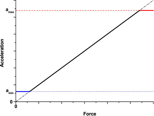
Figure 1: Non-relativistic fundamental principle of dynamics integrating an upper quantum limit when $a>a_{max}$ and a lower limit when $a<a_{min}$. The linear part is plotted for $m=1$.

In that case, the figure 1 is picturing a law that shows strong discontinuities when ${a\leq a_{min}}$ and ${a\geq a_{max}}$. Astronomical observations suggest that such discontinuities are not realistic and that the transition between the two regimes of acceleration is soft. In general, galaxy velocity curves do not show steep growth when ${a\rightarrow a_{min}}$. We need to find a law of dynamics which is continuous and eliminates the discontinuities at $a=a_{min}$ and $a=a_{max}$ by a smooth transition. Furthermore, the previous demonstrations are fairly heuristic and call on the relativistic quantity $E=mc^{2}$ while the quantum physics involved is non-relativistic. Conversely, the previous demonstrations pertain to quantum systems and one could seek to more general systems. A more formal derivation could help to resolve these points.

2.4 Fundamental dynamics principles reshaped by quantum bounds

With this objective in mind, it is proposed to insert quantum bounds on acceleration into the principles of dynamics by using special relativity. Special relativity is suitable for treating accelerations produced by any force, except for strong gravitational regimes. For the moment, we consider a force in the general sense of the definition without specifying its nature, and we try to derive a general expression of the principle of dynamics. Acceleration in special relativity has been extensively studied, notably by Rindler who described the motion of a uniformly accelerated rod [60]. This demonstration lays on the clock hypothesis, which is a generally accepted assumption that the time dilation affecting a clock’s rate does not depend on the acceleration, but only on the instantaneous velocity. This effect has been experimentally verified [67, 68]. However, several studies on maximal (proper) acceleration emphasize that the clock hypothesis may be violated and that Lorentz transformations could be insufficient to describe accelerating observers in special relativity [51, 45, 69, 55]. This point will be presented in the Discussion section.
In special relativity, the proper acceleration $\alpha$ is the acceleration experienced by an object of mass $m$ and measurable with an accelerometer, which measures the quantity $\boldsymbol{\alpha}=\mathbf{F}/m$, where $\mathbf{F}$ is the proper force. Thus, proper acceleration is relative to an inertial observer who is instantly and momentarily at rest relative to the accelerated object. The proper acceleration is different from the coordinate acceleration a which is dependent on the chosen coordinate system. The proper acceleration for uni-directional constant acceleration can also be expressed using other parameters:

$$\boldsymbol{\alpha}=c\frac{d\boldsymbol{\eta}}{d\tau}=\gamma^{3}\frac{d\boldsymbol{v}}{dt}=\gamma^{3}\boldsymbol{a},$$ (35)

where $\boldsymbol{\eta}$ is the rapidity, $\gamma=(1-v^{2}/c^{2})^{-1/2}$ is the Lorentz factor and $\boldsymbol{v}$ is the coordinate velocity. Moreover, rapidity is also defined as

$$\boldsymbol{\eta}=\text{atanh}\left(\frac{{v}}{c}\right)\boldsymbol{\hat{v}},$$ (36)

with $\boldsymbol{\hat{v}}=\boldsymbol{v}/|v|$. The integration over $\tau$ of the first expression of (35) leads to

$$\boldsymbol{\eta}=\frac{\boldsymbol{\alpha}\tau}{c},$$ (37)

and injecting (37) in (36) gives

$$\boldsymbol{v}=c\ \text{tanh}\left(\frac{\alpha\tau}{c}\right){\hat{\boldsymbol{\alpha}}},$$ (38)

with $\hat{\boldsymbol{\alpha}}=\boldsymbol{\alpha}/|\alpha|$. Now that we have an expression for the coordinate velocity $v$, we can obtain the coordinate acceleration $a$ with the time derivative with respect to $t$. However, the right-hand term has no explicit dependence in $t$, and $v$ has no explicit dependence on $\tau$. We can yet write:

$$\frac{d}{dt}\left(\frac{dt}{d\tau}\boldsymbol{v}\right)=\frac{d}{d\tau}c\ \text{tanh}\left(\frac{{\alpha}\tau}{c}\right){\hat{\boldsymbol{\alpha}}}.$$ (39)

By definition, $\gamma={dt}/{d\tau}$ and with an algebraic development ${d(\gamma v)=\gamma^{3}dv}$. The dependence on $\gamma^{3}$ can change if the acceleration is not parallel to velocity. However, for the longitudinal acceleration we obtain:

$$\gamma^{3}\boldsymbol{a}=c\frac{d}{d\tau}\text{tanh}\left(\frac{{\alpha}\tau}{c}\right){\hat{\boldsymbol{\alpha}}}.$$ (40)

At this point, the main novelty of the demonstration is to consider that the special relativity proper time and the quantum speed limit (22) previously introduced are equal. Against this assumption, it could be argued that the quantum speed limit is not suitable for classical systems, but contrary to some common beliefs, classical systems are also concerned with a non-zero speed limit even in the limit $\hbar\rightarrow 0$ [70, 71]. The connection between the quantum speed limit and classical speed limit presents many subtleties, as depicted in the bibliography of [72]. Because no assumption is made on the nature of the accelerated system, for simplicity and without loss of generality, we will merely consider the Levitin and Margolus speed limit, and use it to discretize the special relativity proper time $\tau$. The definition of the maximum acceleration limit depends on the mass of the system and can therefore be extremely high for astrophysical objects. However, in the results section, the examples used are all concerning the minimum acceleration. Thus, the question of whether use the quantum speed limit or the classical speed limit has no consequence in the scope of this study and this is why we use a general case. Indeed, except in the vicinity of a black hole, it is unlikely that we will be able to detect astrophysically the effect of the maximal acceleration limit. In this case, the study of Rovelli and Vidotto [33] is a pioneering work.
The proposed equivalence between special relativity proper time and quantum speed limit imposes that we cannot consider the formal definition of the derivative:

$$\frac{df}{d\tau}\bigg{|}_{\tau=\tau_{0}}=\lim_{\Delta\tau\to 0\atop\Delta\tau\neq 0}\frac{f(\tau_{0}+\Delta\tau)-f(\tau_{0})}{\Delta\tau},$$ (41)

because $\Delta\tau$ does not tend to $0$, but to the quantum proper time $\Delta\tau=\pi\hbar/2mc^{2}$.
In this scheme, we assume that at time $t_{0}=\tau_{0}=0$, the observer and the object share the same inertial frame of reference. The acceleration is constant during a time $\Delta\tau$, and at the end of this time, one can see that the speed of the object has changed. At this moment, knowledge of the instantaneous velocity $v$ is sufficient to determine the time dilation according to the clock hypothesis. Then, if the object undergoes a new acceleration (which is not necessarily the same as the previous one), the situation is identical to the beginning, and an observer can once again be momentarily at rest in the frame of the accelerated object at the beginning of this new acceleration boost. This acceleration is constant during a time $\Delta\tau$ and it gives a new instantaneous velocity to the object, and so on. Thus, we can write the coordinate acceleration (40) as:

$$\boldsymbol{a}=\frac{1}{\gamma^{3}}\frac{c}{\Delta\tau}\text{tanh}\left(\frac{{\alpha}\Delta\tau}{c}\right){\hat{\boldsymbol{\alpha}}}.$$ (42)

Then, if one equates the quantum proper time and the special relativity proper time, we obtain:

$$\boldsymbol{a}=\frac{1}{\gamma^{3}}\frac{2mc^{3}}{\pi\hbar}\text{tanh}\left(\frac{\pi\hbar{F}}{2m^{2}c^{3}}\right){\hat{\boldsymbol{F}}},$$ (43)

with $\hat{\boldsymbol{F}}=\mathbf{F}/|F|$. One can see that the quantity ${2mc^{3}/\pi\hbar}$ is actually the definition of the Caianiello maximal acceleration [36] and that the coordinate acceleration naturally incorporates the upper acceleration quantum bound in the principle of dynamics once the minimal time of evolution and the (relativistic) proper time are equated. We can even write the contracted form as:

$$\boldsymbol{a}=\frac{1}{\gamma^{3}}\ a_{max}\ \text{tanh}\left(\frac{{F}}{ma_{max}}\right){\hat{\boldsymbol{F}}}.$$ (44)

Now, we must include also the lower quantum bound $a_{min}$. To do that, we first have to remember the properties of such a quantum bound. The position-momentum uncertainty principle defines the minimum permitted momentum regarding to uncertainty of the position [61], and thus the maximum de Broglie wavelength, which is limited by the size of the observable Universe. From this, if the velocity is equal to $c$, the minimum possible mass is $m_{min}=\hbar/2cR_{u}$ and the associated speed limit (22) is:

$$\Delta\tau=\frac{\pi R_{u}}{c}.$$ (45)

The different properties associated to the two acceleration bounds used in the model are summarized in the table 1.

	Quantum speed limit	Acceleration limit	Associated $\lambdabar_{dB}$
Max. bound	$\Delta\tau={\pi\hbar}/{2mc^{2}}$	$a_{max}={2mc^{3}}/{\pi\hbar}$	$\lambdabar_{dB}={\hbar}/{mc}$
Min. bound	$\Delta\tau={\pi R_{u}}/{c}$	$a_{min}={c^{2}}/{\pi R_{u}}$	$\lambdabar_{dB}={\hbar}/{p_{min}}=2R_{u}$

Table 1: Properties associated to minimal and maximal bounds on dynamics.

This time (45) is then the proper time used to derive the minimal acceleration term. Using the same demonstration as before, we can find

$$\boldsymbol{a}=\frac{1}{\gamma^{3}}\frac{c^{2}}{\pi R_{u}}\text{tanh}\left(\frac{c^{2}{F}}{\pi mR_{u}}\right){\hat{\boldsymbol{F}}}=\frac{1}{\gamma^{3}}a_{min}\text{tanh}\left(\frac{{F}}{ma_{min}}\right){\hat{\boldsymbol{F}}}.$$ (46)

One could argue that the minimal acceleration has not a quantum nature since $\hbar$ does not clearly appear in the expression of $a_{min}$. This is actually contained in the expression of $R_{u}$ which is equal to the de Broglie wavelength.
We now examine the boundary conditions to articulate these two competing effects. Figure 1 suggests that maximal acceleration and minimal acceleration terms must reproduce the Newtonian law of dynamics once together, excepted for very low and very high accelerations. It is proposed to write the equation as the sum of these two effects, on the basis of the equation (44):

$$\boldsymbol{a}=\frac{1}{\gamma^{3}}\ \left\{\kappa a_{max}\ \text{tanh}\left(\frac{{F}}{ma_{max}}\right)+\beta a_{min}+\epsilon\right\}{\hat{\boldsymbol{F}}},$$ (47)

where $\kappa$, $\beta$ and $\epsilon$ are functions or coefficients to be determined. The first condition is given by the boundary condition ${F\rightarrow+\infty}$, for which we should have ${a\rightarrow a_{max}/\gamma^{3}}$, and not ${a\rightarrow(a_{max}+a_{min})/\gamma^{3}}$, otherwise it would violate the maximal permitted acceleration. Thus, it follows that $\kappa=+1$ and that $\beta a_{min}+\epsilon=0$ for $F\rightarrow+\infty$. The second condition for the limit ${F\rightarrow 0}$ imposes that ${a\rightarrow a_{min}/\gamma^{3}}$ and which leads to $\beta=+1$ and $\epsilon(F=0)=0$, because the first term of (47) vanishes.

Finally, by identification it appears that $-\epsilon=a_{min}\text{tanh}(F/ma_{min})$ is given by equation (46). Moreover, it is possible to start on the basis of equation (46)

$$\boldsymbol{a}=\frac{1}{\gamma^{3}}\ \left\{\delta a_{min}\ \text{tanh}\left(\frac{{F}}{ma_{min}}\right)+\zeta a_{max}+\chi\right\}{\hat{\boldsymbol{F}}},$$ (48)

with $\delta$, $\zeta$ and $\chi$ coefficients or functions to be determined. The same boundary conditions lead to $\delta=-1$, $\chi=a_{min}$ and $\zeta=\text{tanh}(F/ma_{max})$. Thus, by deduction, the equation governing the dynamics limited by quantum bounds can be written as follows:

$$\boldsymbol{a}=\frac{1}{\gamma^{3}}\left\{a_{max}\ \text{tanh}\left(\frac{F}{ma_{max}}\right)+a_{min}\left[1-\text{tanh}\left(\frac{F}{ma_{min}}\right)\right]\right\}{\hat{\boldsymbol{F}}}.$$ (49)

Equation (49) is plotted in figure 2, with a zoom near $F=0$, close to the minimal acceleration quantum bound.

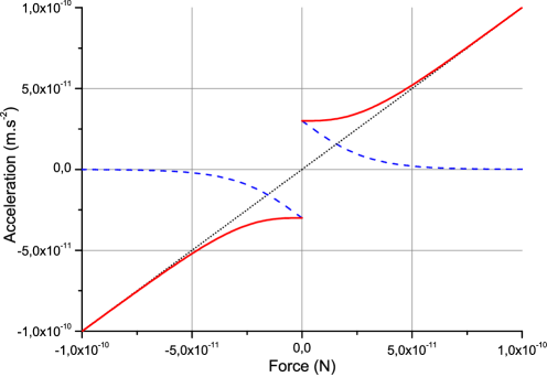
Figure 2: Plot of the two different terms of equation (49) for $m=1$ and $R_{u}=10^{27}$ m. The black dot lines is the plot of first term associated to the maximal acceleration bound. The blue dashed line is the plot of the second term assigned to minimal acceleration limit. The continuous red line is the sum of the two.

Consequently, equation (49) defines a new principle of dynamics, in which the relation of proportionality between the force and acceleration is fundamentally broken. With these combinations of two hyperbolic tangents, we can identify three acceleration regimes:

• The first regime is Newtonian and appears if ${ma_{min}\ll F\ll ma_{max}}$. In this case, the principle of dynamics is almost identical to that of Newton, and the dynamics are well approximated by $a=F/m$. While the minimal acceleration term vanishes, the proportionality relation $a=F/m$ is ensured by the hyperbolic tangent function properties, since ${\text{tanh}(x)=x}$ when ${x\rightarrow 0}$, recovering the classical limit if $v\leavevmode\nobreak\ <<\leavevmode\nobreak\ c$.

• The second regime involves an applied force that is close to the maximal acceleration bound. The dynamics enter a Caianiello acceleration regime, where
  ${F\sim m\,a_{max}}$. Newton’s law no longer applies and the acceleration of the body becomes less and less strong even if the applied force increases indefinitely. At some point, the acceleration is locked at the value $a_{max}$ even if ${F\rightarrow\infty}$.

• The third regime, more described in this paper, appears when $F\sim m\,a_{min}$. Symmetrically to the Caianiello regime, the acceleration is no longer proportional to the applied force, but begins to smoothly saturate at a value $a_{min}$ as $F\rightarrow 0$. In figure 2, we can see that when $F$ is decreasing, the minimal acceleration term plotted in the dashed blue line becomes dominant whereas the maximal acceleration term in the dotted black line tends to 0 quasi linearly, because this is the maximal term that approximates the typical Newtonian relation $a=F/m$.

3 Results

The first application of the dynamical law (49) is the prediction of galaxy rotation curves. For example, the terminal centripetal accelerations of hydrogen clouds measured for a collection of 22 motley spirals [73] are plotted on the figure 3. The orbital velocities range from ${54\ \text{km/s}}$ to ${300\ \text{km/s}}$ and their masses scale rather precisely with the velocity.

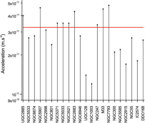
Figure 3: Stars are the centripetal accelerations corresponding to rotational velocity at outermost radius for a sample of 22 galaxies extracted from [73]. The solid red line is an approximate value of the minimal acceleration (32) calculated with the $\Lambda$CDM radius of the observable Universe. Galaxies are classified according to their terminal velocity.

The main insight drawn from figure 3 is that the acceleration of stars never falls deeply below $a_{min}$, regardless of the mass of the galaxy or its luminosity. For example, in this sample of 22 galaxies, the lower terminal centripetal accelerations are given by NGC 1003 at ${1.2\times 10^{-11}\text{m s}^{-2}}$. It is possible to find even slightly lower accelerations in other catalogs, but we have to keep in mind that the observations are strongly dependent on the orbits of hydrogen clouds that are not always circular or are not perfectly orbiting in the plane of galactic discs and can even orbit in galaxies tidally interacting with other galaxies or in warped galaxies, like NGC 1003. Furthermore, the velocity measured at the outermost radius is not always completely due to the minimal acceleration and a residue of gravitational interaction can still substantially contribute. Thus, if one wants to precisely measure the minimal acceleration, the only way is to find some very isolated galaxies, with a thin disc, if possible with stars or detectable HI or HII clouds on circular orbits at the outskirt. Though, we can still estimate $a_{min}$ by calculating the mean of the terminal accelerations extracted from [73] and plotted on the figure 3:

$$a_{min}\simeq 3\times 10^{-11}\ \text{m s}^{-2}$$ (50)

This value is consistent with the estimation ${a_{min}\sim 3\times 10^{-11}\text{m s}^{-2}}$ calculated with the $\Lambda$CDM observable Universe radius. The mean terminal centripetal acceleration from [73] is approximative because the uncertainties are not determined for the above-mentioned reasons.
However, the bibliography about rotation curves of galaxies is extremely wide and we can test the model on more precise examples, although we limit the study to objects with circular or quasi-circular orbits. If one assumes that a star has a circular orbit and that gravitation in a weak field is well described by the Newtonian law $\textbf{F}=-GMm\hat{\boldsymbol{r}}/r^{2}$ with $\hat{\boldsymbol{r}}=\boldsymbol{r}/|r|$ , the circular velocity is given by a simple application of the equation $a=v^{2}/r$:

$$\boldsymbol{v}=\sqrt{\frac{r}{\gamma^{3}}\left\{a_{max}\text{tanh}\left(\frac{GM}{a_{max}r^{2}}\right)+a_{min}\left[1-\text{tanh}\left(\frac{GM}{a_{min}r^{2}}\right)\right]\right\}}\ \hat{\boldsymbol{r}}.$$ (51)

For small speeds $v\ll c$ and in the low acceleration regime, as we are in weak gravitational field, the hyperbolic tangent reduces to $\text{tanh}(GM/a_{max}r^{2})\rightarrow GM/a_{max}r^{2}$ when $|GM/a_{max}r^{2}|\rightarrow\leavevmode\nobreak\ 0$. Thus, we get:

$$\boldsymbol{v}=\sqrt{\frac{GM}{r}+ra_{min}\left[1-\text{tanh}\left(\frac{GM}{a_{min}r^{2}}\right)\right]}\ \hat{\boldsymbol{r}}.$$ (52)

Compared with the highly complex dynamics of real galaxies, this equation is very simple and its purpose is to create a toy model useful for roughly testing some observations. First, as we treat the galaxy mass as a single point, this formula describes the orbital velocity of stars that are far from the galactic bulge. Because the aim of this application is to explore the regime of $F\sim m\,a_{min}$, this condition is satisfied. Furthermore, if one wants to test the principle of dynamics proposed here on an entire rotation curve, it is necessary to consider the density profile of the corresponding galaxy. At present, we consider the effect of a minimal acceleration on the galaxy rotation curves where gravitation is very weak, in the outskirts of the galaxy discs.
Owing to the third data release of the Gaia mission (Gaia DR3) [74], it has recently been pointed out that the Milky Way (MW) rotation curve shows a Keplerian decline at a distance from 15 kpc to 27 kpc from the center [75, 76]. This observation strongly reduces the mass of the total MW to ${M_{MW}=2.06_{-0.13}^{+0.24}\times 10^{11}M_{\odot}}$. In figure 4, the rotation curve measured in [75] is reproduced, and the theoretical rotation curve from Eq. (52) is plotted for the lower and upper bounds of the MW mass. The plot begins at 16 kpc, far from the bulge, and the theoretical rotation curve is in good agreement for the lower bound of the MW mass $M_{MW}=1.93\times 10^{11}M_{\odot}$, although the galaxy mass is treated as a point instead of a galaxy profile.

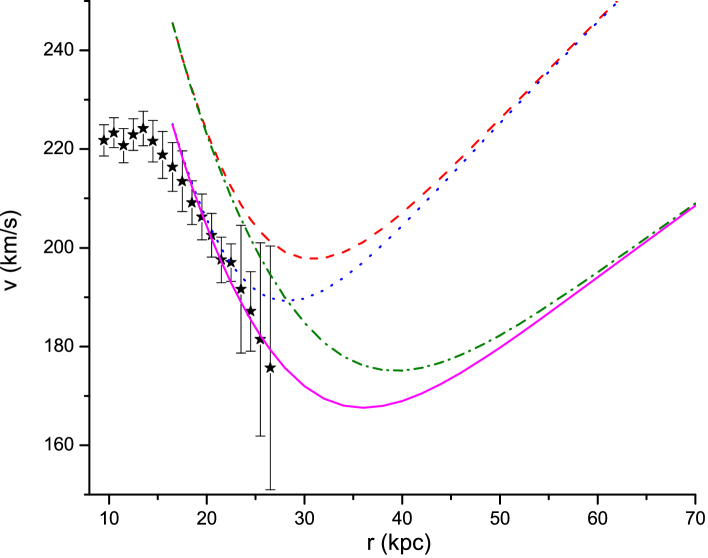
Figure 4: Plot of the velocity curve as function of the distance from the center of the Milky Way. Experimental data from [75] is represented by stars with error bars. The theoretical velocity from the equation (52) is plotted in red dashed line for highest MW mass ${M_{MW}=2.30\times 10^{11}M_{\odot}}$ and $a_{min}=3.3\times 10^{-11}$ m s^-2, in blue dotted line for smallest MW mass ${M_{MW}=1.93\times 10^{11}M_{\odot}}$ and $a_{min}=3.3\times 10^{-11}$ m s^-2, in green dashed dotted line for highest MW mass and ${a_{min}}=2\times 10^{-11}$ m s^-2 and finally in purple solid line for smallest MW mass and ${a_{min}}=2\times 10^{-11}\text{m s}^{-2}$.

Formula (52) predicts that the velocity of far objects orbiting around the MW should increase, contrary to MOND theory which predicts a flat velocity curve at long distance [20]. On the outskirts, the model also predicts that the speed is independent of the galaxy mass, because it is almost entirely governed by $a_{min}$. One can see that the model is strongly dependent on the value of $a_{min}$ at long distance and of the mass of the galaxy at short distance. For the value of $a_{min}=2\times 10^{-11}$ m s^-2, the model predicts that the MW rotation curve decreases at least until 35 - 40 kpc and increases again. The scale is zoomed around 200 km/s, giving the impression that the velocity strongly varies, nevertheless the velocity is quasi flat between 20 and 60 kpc with a variation of only 20 km/s. Furthermore, a single point mass is considered in the model, which likely leads to a truncation of the flat part of the rotation curve, compared to a real density profile.
Nevertheless, the experimental data stops at 27 kpc, and if one wants to study the velocity curve at a long distance, it is necessary to find celestial objects orbiting further away. For this purpose, the Gaia mission could be relevant, as it allows the observation of ultra faint galaxy satellites of the MW (UFMW) at large distances [77, 78]. If one looks at the orbital parameters of the UFMW satellites in [77], it is clear that they are moving at very high velocities ($\sim 200-400$ km/s), easily exceeding the maximal velocity measured before the Keplerian decline (224 km/s), as suggested by the model. However, a rough estimation of the velocities must be tempered by the limited knowledge of the orbitals parameters of these ultra faint galaxies and the eccentricity of these celestial bodies which is often quite important. Moreover, the interaction of the UFMW satellites between each other and with other galaxies such as the Magellanic clouds has to be taken in account.
However, for dwarf spirals, the rotation curve appears to increase monototically. This behavior seems to be common in dwarf spirals, and a universal rotation curve was synthesized by Karukes and Salucci [79]. This synthetic curve is reproduced in figure 5, and the data are fitted using equation (52). As the mass of the dwarf galaxies is small, it can be assumed that the centripetal acceleration due to Newtonian gravitation is smaller than $a_{min}$ over the entire rotation curve, and thus neglect the mass of the galaxy by choosing $M=0$. Equation (52) is then reduced to:

$$\boldsymbol{v}=\sqrt{ra_{min}}\ \hat{\boldsymbol{r}},$$ (53)

and provides the minimal velocity rotation curve. The fitting of the synthetic data by equation (53) is in very good agreement with $a_{min}\approx 2\times 10^{-11}\text{m s}^{-2}$, showing that the model also works for dwarf galaxies. The value of $a_{min}$ is slightly lower than the value measured for [73], but is still in agreement. The fitting of the dwarf universal rotation curve with $M=0$ corroborates the recent claim that the stellar dynamics of dwarf galaxies are completely dominated by the putative dark matter halo [80].

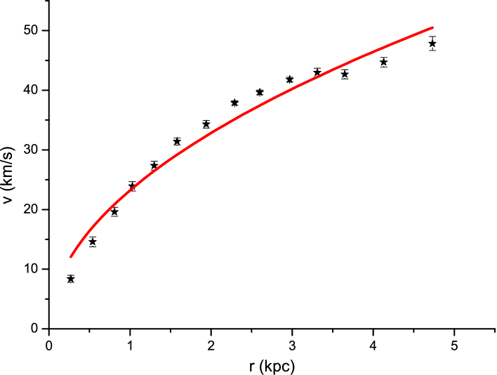
Figure 5: Stars with error bars are the synthetic universal rotation curve of dwarf galaxies modeled by E. V Karukes and P. Salucci [79]. The red curve is a fitting of experimental data with equation (53).

The measurement of $a_{min}$ could perhaps be performed more conveniently in galaxies isolated for a long time, with no interaction with other celestial bodies. The recently discovered superthin galaxies may be a suitable laboratory to measure $a_{min}$, since these galaxies have some interesting properties: stars with quasi-circular orbits and superthin discs, meaning that the vertical motion (orthogonal to the disc) of stars is very small, extended rotation curves, motley masses, and a weak spheroidal component. Bizyaev et al. carried out an important study of 138 superthin galaxies and plotted their rotation curves [81]. It is worth noting that most of the rotations curves do not have a flat velocity at long distance, and for many of them the velocity increases monotonously.

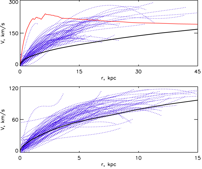
Figure 6: Figure extracted from [81] with the courtesy of D. Bizyaev. Dashed blue lines are the rotation curves of 138 superthin galaxies, for maximal velocities ${v>120\ \text{km/s}}$ in the upper panel and ${v<120\ \text{km/s}}$ in the lower panel. Red continuous line is a previous Milky Way rotation curve, extracted from [82] by the authors. Black continuous lines are plotted from equation (53) and added to the original figure of [81].

Black lines in figure 6 are the plots of equation (53), with neglecting the mass of galaxies, and with a minimal acceleration ${a_{min}=2\times 10^{-11}\text{m s}^{-2}}$ obtained by the fitting of dwarf galaxies on figure 5. It is expected that the rotation curves are always above the minimal velocity ${v=\sqrt{a_{min}r}}$. In the lower panel, almost all the curves are above and behave with the root of distance to center of galaxy. In the upper panel, almost all the rotation curves are also above the minimal velocity curve. This result was expected since velocities are inevitably underestimated with choosing $M=0$. Thus, the model seems to describe correctly the rotation curves of superthin galaxies, independently of their masses. Still in [81], the case of UGC 7321 is more finely studied, but this galaxy disc is known to have a warp beginning near the edge of stellar disc [83]. Nevertheless, latest points of the velocity curves are globally in agreement with $a_{min}$. Decreasing or fluctuating rotation curves suggests an asymmetric velocity, which may indicate the presence of a bar in the galaxy disc or strong spiral arms. However, the absence of error bars makes difficult to discuss further the agreement between the model and observations.
Many galaxy rotation curves also do not grow and are neither flat, and show a pronounced decline. This could appear to contradict the model that predicts the growth of velocity, however, the velocity increases with distance only if the centripetal acceleration is very close or equal to $a_{min}$. Zobnina and Zasov studied the rotation curves of 22 spirals having a declining curve at long distance [84]. For 17 of the 22 spirals in the study, centripetal acceleration was greater than the theoretical value of $a_{min}$, and approximately equal to $a_{min}$ for 2 galaxies. Only 3 spirals on 22 exhibit a centripetal acceleration lower than $a_{min}$, which is still compatible with the value of $a_{min}=2\times 10^{-11}\text{m s}^{-2}$ found with dwarf galaxies for NGC 5055 and NGC 2599, and slightly lower ($a=1.13\times 10^{-11}\ \text{m s}^{-2}$) for NGC 157. Nevertheless, NGC 5055 and NGC 157 have pronounced warps correlated with a circular velocity drop [85, 86] and NGC 2599 is close to face-on which leads to significant errors on the rotations velocities [87].
Four types of galaxies are considered in this study: spirals, especially the Milky Way, dwarf galaxies, superthin galaxies and decreasing rotation curve galaxies. However, it is possible to enlarge and summarize these galaxy rotation curves, with a radial acceleration relation with accelerations ranging from $10^{-14}$ to $10^{-8}$ m s^-2. Figure 7 extracted from [25] reproduces this radial acceleration relationship. In addition to the deviation from the Newtonian law, the authors of [25] suspect the existence of a ”flattening” of the acceleration at a value estimated close to $9\times 10^{-12}$ m s^-2, which is quite close to $a_{min}=2\times 10^{-11}$ m s^-2. The general behavior of the radial acceleration relation seems notably well described by the present model, as shown by the blue curve in figure 7. The blue curve is not a fit, but a simple plot of the expected acceleration given by equation (49) and the value $a_{min}=2\times 10^{-11}$ m s^-2 obtained with the data of [79].

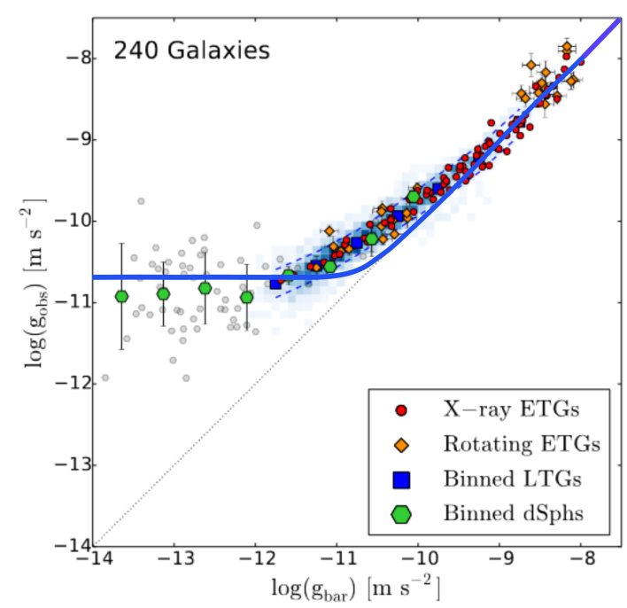
Figure 7: Figure extracted from [25] with the courtesy of F. Lelli. Plot of the radial acceleration relation considering several galaxy types. The color scale represents  2700 points from 153 late-type galaxies: blue squares and dashed lines show the mean and standard deviation of the binned data, respectively. Red circles and orange diamonds indicate rotating early-type galaxies (ETGs) and X-ray ETGs, respectively. Small gray hexagons show dwarf spheroidals and large green hexagons show the mean and standard deviation of binned data. The continuous large blue curve is the acceleration predicted by equation 49 of the model.

While the Newtonian and minimal acceleration regimes are in agreement with the model, the intermediate regime seems to be less well described. However, SPARC data are strongly dependent on the stellar-to-mass ratio and the shape of the radial acceleration relation varies as a function of the chosen galactic parameters. This leads to an uncertainty of $\sim$20 % in the knowledge of the MOND acceleration scale according to the authors of [25]. Furthermore, it was recently shown that the RAR proposed by MOND is in tension with the Cassini-Huygens probe trajectory. The probe data exclude the deviation from the Newtonian regime near $g_{bar}=10^{-10}$ m s^-2 [88], while the present model is in accordance.
In summary, for massive spiral galaxies with a bulge, a rapid rise in the velocity followed by a Keplerian decline can be observed. After this decline, the formula predicts that the velocity will stabilize while the Newtonian gravitation gradually gives way to the minimal acceleration term, and thereafter the velocity increases again with the distance. It is suggesting that this minimal acceleration dominates far away from the bulge, in the outskirts of massive galaxies. The flat part of the curve for spirals can vary as a function of the distribution of baryonic matter because the Keplerian decline can compensate for the growth of the centripetal acceleration due to the minimal acceleration term in (49).
At long distances, all the rotation curves converge. A similar toy model was previously proposed by Grumiller and Preis [89], but its velocity equation is empirical although it has some similarities with equation (52). However, this violates the maximal acceleration bound and overestimates the effect of the minimal acceleration quantum bound.

4 Discussion

4.1 Potentials associated to minimal and maximal accelerations

The demonstration of the maximal acceleration proposed by Caianiello relies on uncertainty principles and the Ehrenfest theorem. Indeed, a velocity operator $\hat{v}$ is introduced with the latter, and equation (11) which is the cornerstone of Caianiello’s demonstration. Interestingly, this demonstration could also imply the existence of quantum bound related position-dependent potentials. From the Ehrenfest theorem, we can write:

$$\langle\Psi|[\hat{v},\hat{H}]|\Psi\rangle = \frac{1}{m}\langle\Psi|[\hat{p},\hat{H}]|\Psi\rangle$$ (54)

$$= \frac{1}{m}\langle\Psi|[\hat{p},\frac{\hat{p}^{2}}{2m}+V(r)]|\Psi\rangle,$$ (55)

where $V(r)$ is the potential. Because $\hat{p}$ commutes with itself, in the case of $V(r)=0$, the equation reduces to 0 and the maximal acceleration bound disappears.
However, the above relativistic demonstration is developed out of any particular quantum states and naturally implies the existence of acceleration bounds, when introducing the equivalence between speed limit and relativistic proper time. This suggests the presence of potentials corresponding to maximal and minimal accelerations. Futhermore, Feoli et al. [90] have shown that the maximal acceleration can be embedded into the Schwarzschild metric leading to an effective potential, meaning that both minimal and maximal accelerations could be expressed as corrections in a Schwarzschild metric.

4.2 A dependence to the redshift?

Here, the minimal acceleration is presented as a universal constant, in the sense that its value should be everywhere the same because of the isotropy of space and the homogeneity of the observable Universe at large scale. However, does $a_{min}$ remain constant over cosmic time ? As it directly depends on the radius of the observable Universe, this could mean that its value decreases with time and, conversely, that $a_{min}$ was greater in the past.
Let us consider the scale factors $a_{S}(t_{0})$ and $a_{S}(t)$, respectively at the present epoch $t_{0}$ and at any other epoch $t$, depending on the redshift $z$:

$$\frac{a_{S}(t_{0})}{a_{S}(t)}=1+z.$$ (56)

We can thus define the radius of the observable Universe at any time with:

$$\frac{R_{u}(t)}{R_{u}(t_{0})}=\frac{a_{S}(t)}{a_{S}(t_{0})}.$$ (57)

Using equations (56) and (57), we can express the redshift as a function of $R_{u}(t_{0})$ and $R_{u}(t)$:

$$z=\frac{R_{u}(t_{0})}{R_{u}(t)}-1.$$ (58)

Moreover, the value of $a_{min}$ theoretically depends on the radius of the observable Universe

$$a_{min}(t)=\frac{c^{2}}{\pi R_{u}(t)},$$ (59)

so we can express $a_{min}(t)$ as a function of the redshift:

$$a_{min}(t)=\frac{c^{2}(1+z)}{\pi R_{u}(t_{0})}.$$ (60)

Consequently, it appears that $a_{min}$ varies linearly with the redshift $z$ and it is expected that $a_{min}$ was greater during the early Universe. The Magneticum collaboration [91] depicts the evolution of the MOND acceleration scale $a_{0}$ with $z$ and observe a constant decrease of $a_{0}$ with $z$. Although the mondian $a_{0}$ scale factor and $a_{min}$ are conceptually different, it can leave a hint concerning the evolution of $a_{min}$ with the redshift.
Furthermore, the formation of early galaxy discs could also reveal some different features in the presence of a stronger minimal acceleration, compared with the ${\Lambda}$CDM model.

4.3 Quantum bounds acceleration dynamics and the Tully-Fisher relation

The empirical Tully–Fisher relation establishes a relationship between the intrinsic luminosity (or mass) of a spiral galaxy and its asymptotic rotation velocity. Brightness is proportional to $v^{\alpha}$, with $\alpha$ close to 4, depending on the observed wavelength [92]. In the infrared domain, the total luminosity of the galaxy is approximately proportional to the mass of stars. Therefore, we deduced that the stellar mass is proportional to $v^{4}$. MOND predicts this relationship by considering $v$ as the speed limit at large $r$ [93]. However, from an observational point of view, the measured velocity is not necessarily the velocity at high radius $r$, but rather the maximum velocity.
In the proposed model, at first glance it is not possible to find a formula with $v$ constant at a long distance because $v$ continues to grow with $r$ owing to the minimal acceleration, as described by equation (53). However, in the low-acceleration regime, the increase in $\sqrt{r}$ is quite slow, and where the optical disk ends, the velocity can give the impression of tending towards an asymptotic value. This flattening effect of the velocity is enhanced by decreasing gravity in $r^{2}$, as mentioned in the previous section, in which the rotation curve of the Milky Way is quasi flat ($\pm$ 20 km/s) from 20 to 60 kpc. However, this question is interesting and deserves to be explored further.

4.4 Clock hypothesis

From a theoretical point of view, one major difference between this study and others related to maximal acceleration is that the present demonstration lays on the clock hypothesis. Other studies suggest that the clock hypothesis is no longer valid [51, 45, 69, 55] and consider that Lorentz transformations have to be modified to consider the acceleration in the time-dilation effect, leading to a new relativity theory. In the present study, it is assumed that the proper acceleration is proportional to the proper force $F$, and that $F$ can take an arbitrarily large value, at least up to the Planck force $c^{4}/G$. For all particles lighter than the Planck particle, nothing prevents someone from applying a force larger than $F_{max}=m\ a_{max}$. For that reason, this demonstration focuses on the proper force to establish that a limitation on the coordinate acceleration appears naturally when the quantum time of evolution and the relativistic proper time are equal. Thus, for external observers, the dynamics of the accelerated objects is effectively limited by $a_{min}$ and $a_{max}$. The originality of this article compared to the other works mentioned above is that the relation (49) integrates the two quantum bounds, without renouncing the clock hypothesis. It should be noted that the Rovelli and Vidotto study of maximum acceleration in quantum loop gravity [33] also respects this principle.
However, it is clear that this model is probably not complete because we are treating the gravitation as a Newtonian force. Equation (49) should be suitable for a majority of situations except in the strong gravity regime, because uncertainty principles are suspected to be modified in strong gravitational fields [94]. Furthermore, the model may not be suitable for very long distances comparable to the Hubble radius, for which we probably need a generalized theory. Nevertheless, the principle of dynamics (49) is sufficient to deal with the galaxy rotation curves because stars have weak gravitational interactions in galaxies and the considered galaxy radii are very small compared to the Hubble radius.

4.5 The case of F=0

Among the features of this model, figure 2 shows that a discontinuity appears at $F=0$. However, the acceleration defined in equation (49) is a vector. Consequently, in the absence of a force, it is not possible to precisely define the direction of this minimal acceleration. For the scope of this study, there is always a field that provides a preferred direction for $\boldsymbol{a_{min}}$, therefore, there is no practical consequence. For example, in the case of galaxy rotation curves, it is clear that the $\boldsymbol{a_{min}}$ vector is aligned with the centripetal acceleration due to gravity, and this should be the case for all the rotation curves unless another gravitational field appears to be stronger. Thus, under the scope of the galaxy rotation curves, the model is suitable, but resolving the case $F=0$ may require a generalized theory. This question is also present in MOND, depending on which interpolation function is used. For example, the MOND interpolation function that is used to fit the previous radial acceleration relation

$$g_{obs}=\frac{g_{bar}}{\sqrt{1-\text{exp}(g_{bar}/a_{0})}}$$ (61)

presents an undefined solution when $g_{bar}=0$.

4.6 Universality of the minimal acceleration ?

Finally, the application examples of the minimal acceleration are all related to galaxy rotation curves and thus to gravity. This could suggest that the quantum bound on acceleration concerns gravity exclusively. In fact, regarding the maximal acceleration bound, several applications proposed in the literature are not only related to gravity but also not exhaustively to the spin of particles [95], gravitation and electric field [59], and corrections of the Lamb shift [49]. As the minimum and maximal acceleration bounds are symmetric, it seems that there is no justification to restrict the minimal acceleration to gravity. Both quantum bounds on acceleration presumably apply to all possible forces or interactions and should be considered as a general dynamical effect, independently of the nature of the force applied on the accelerating object. This approach promotes the previous development of a law on dynamics instead of solely searching for a modification of gravitation’s law.

5 Conclusions

In summary, a minimal acceleration quantum bound is proposed, symmetrical to the maximal acceleration found four decades ago [36]. It is suggested to include these two competing effects into a modified inertia model by using the formalism of special relativity and relying on the clock hypothesis. The main assumption for deriving the novel principle of dynamics is to introduce the equivalence between the quantum speed limit and the proper time of the reference frame of the accelerated object. Therefore, upper and lower limitations naturally appear in the coordinate acceleration in this new principle of dynamics.
The most evident example where the minimal acceleration appears to be dominant is in the galaxy rotation curves, because far from the bulge of the galaxies, the acceleration due to (Newtonian) gravity is comparable to $a_{min}$ and even smaller. The most striking point is that the centripetal accelerations seem to be all greater, equal or slightly lower than the theoretical $a_{min}$. Thus, such a minimal acceleration effect has an implication in the dark matter problem, which is subject to a debate between the supporters of the introduction of cold dark matter to conserve the existing law of dynamics and the proponents of the MOND theory, which modifies Newtonian dynamics by the introducing a scale acceleration.
The model presented here is, however, different from the MOND theory because it predicts a minimal acceleration that is conceptually different from the scale acceleration $a_{0}$ of MOND, although $a_{0}$ and $a_{min}$ have rather similar magnitudes. While MOND predicts flat galaxy rotations curves, the present theory suggests that the velocity curve increases monotonously when the Newtonian gravitational contribution to centripetal acceleration is lower than $a_{min}$. This prediction seems to be supported by the very high tangential velocities of the ultra faint galaxies orbiting around the Milky Way [77] and by the monotonously increasing velocity curves in the dwarf and superthin galaxies. Furthermore, the theory presented here is also different to the ”ordinary” cold dark matter that is abundantly distributed in the galaxy discs and far in the outskirts to explain the galaxy rotation curves. Although this theory is not intended to prove the absence of cold dark matter or exotic particles such as axions, we can reasonably expect that the amounts of dark matter necessary to explain the motion of celestial bodies is dramatically lower than expected in this framework.
Regarding the correspondence of the theory presented here with the existing laws of physics, one can see that when the acceleration regime is slightly greater than $a_{min}$, the present model quickly recovers the Einsteinian principles of dynamics, and the Newtonian one $a=F/m$ if the velocity is small. This principle of dynamics is thus very similar to the previous one, and only changes when the acceleration reaches the lower and upper quantum bounds, which are respectively very small (approximately 12 orders of magnitude lower than the Earth’s gravitational acceleration) and very high as a function of the mass of the particle.
Finally, another strong prediction is that this minimal acceleration was probably greater in the past, possibly with a strong impact on the formation of galaxies and other large structures of the Universe.

Data Availability

No new data were generated or analyzed in support of this research.

References

- [1] F. Zwicky, “Republication of: The Redshift of Extragalactic Nebulae,” Gen Relativ Gravit, vol. 41, pp. 207–224, Jan. 2009.
- [2] A. Bosma, The distribution and kinematics of neutral hydrogen in spiral galaxies of various morphological types. PhD thesis, Mar. 1978.
- [3] V. C. Rubin and W. K. Ford, Jr., “Rotation of the Andromeda Nebula from a Spectroscopic Survey of Emission Regions,” ApJ, vol. 159, p. 379, Feb. 1970.
- [4] V. C. Rubin, N. Thonnard, and W. K. Ford, Jr., “Rotational properties of 21 SC galaxies with a large range of luminosities and radii, from NGC 4605 (R = 4kpc) to UGC 2885 (R = 122 kpc),” ApJ, vol. 238, p. 471, June 1980.
- [5] J. G. de Swart, G. Bertone, and J. van Dongen, “How dark matter came to matter,” Nat Astron, vol. 1, pp. 1–9, Mar. 2017. Number: 3 Publisher: Nature Publishing Group.
- [6] P. J. McMillan, “Mass models of the Milky Way,” Monthly Notices of the Royal Astronomical Society, vol. 414, pp. 2446–2457, July 2011.
- [7] C. Krishnan, O. Almaini, N. A. Hatch, A. Wilkinson, D. T. Maltby, C. J. Conselice, D. Kocevski, H. Suh, and V. Wild, “The clustering of X-ray AGN at 0.5 < z < 4.5: host galaxies dictate dark matter halo mass,” Monthly Notices of the Royal Astronomical Society, vol. 494, pp. 1693–1704, May 2020.
- [8] M. Bradač, T. Schrabback, T. Erben, M. McCourt, E. Million, A. Mantz, S. Allen, R. Blandford, A. Halkola, H. Hildebrandt, M. Lombardi, P. Marshall, P. Schneider, T. Treu, and J.-P. Kneib, “Dark Matter and Baryons in the X-Ray Luminous Merging Galaxy Cluster RX J1347.5–1145*,” ApJ, vol. 681, p. 187, July 2008.
- [9] K. Umetsu, “Cluster–galaxy weak lensing,” Astron Astrophys Rev, vol. 28, p. 7, Nov. 2020.
- [10] Z. Chacko, Y. Cui, S. Hong, and T. Okui, “Hidden dark matter sector, dark radiation, and the CMB,” Phys. Rev. D, vol. 92, p. 055033, Sept. 2015.
- [11] M. Safronova, D. Budker, D. DeMille, D. F. J. Kimball, A. Derevianko, and C. W. Clark, “Search for new physics with atoms and molecules,” Rev. Mod. Phys., vol. 90, p. 025008, June 2018.
- [12] J. Yoo, J. Chaname, and A. Gould, “The End of the MACHO Era: Limits on Halo Dark Matter from Stellar Halo Wide Binaries,” ApJ, vol. 601, pp. 311–318, Jan. 2004. Publisher: American Astronomical Society.
- [13] Y. Stadnik and V. Flambaum, “Can Dark Matter Induce Cosmological Evolution of the Fundamental Constants of Nature?,” Phys. Rev. Lett., vol. 115, p. 201301, Nov. 2015.
- [14] L. Roszkowski, E. M. Sessolo, and S. Trojanowski, “WIMP dark matter candidates and searches—current status and future prospects,” Rep. Prog. Phys., vol. 81, p. 066201, May 2018.
- [15] ADMX Collaboration, N. Du, N. Force, R. Khatiwada, E. Lentz, R. Ottens, L. Rosenberg, G. Rybka, G. Carosi, N. Woollett, D. Bowring, A. Chou, A. Sonnenschein, W. Wester, C. Boutan, N. Oblath, R. Bradley, E. Daw, A. Dixit, J. Clarke, S. O’Kelley, N. Crisosto, J. Gleason, S. Jois, P. Sikivie, I. Stern, N. Sullivan, D. Tanner, and G. Hilton, “Search for Invisible Axion Dark Matter with the Axion Dark Matter Experiment,” Phys. Rev. Lett., vol. 120, p. 151301, Apr. 2018. Publisher: American Physical Society.
- [16] E. Savalle, A. Hees, F. Frank, E. Cantin, P.-E. Pottie, B. M. Roberts, L. Cros, B. T. McAllister, and P. Wolf, “Searching for Dark Matter with an Optical Cavity and an Unequal-Delay Interferometer,” Phys. Rev. Lett., vol. 126, p. 051301, Feb. 2021.
- [17] A. Boyarsky, M. Drewes, T. Lasserre, S. Mertens, and O. Ruchayskiy, “Sterile neutrino Dark Matter,” Progress in Particle and Nuclear Physics, vol. 104, pp. 1–45, Jan. 2019.
- [18] J. M. Gaskins, “A review of indirect searches for particle dark matter,” Contemporary Physics, vol. 57, pp. 496–525, Oct. 2016. Publisher: Taylor & Francis _eprint: https://doi.org/10.1080/00107514.2016.1175160.
- [19] G. Bertone and T. M. P. Tait, “A New Era in the Search for Dark Matter,” Nature, vol. 562, pp. 51–56, Oct. 2018.
- [20] M. Milgrom, “A modification of the Newtonian dynamics as a possible alternative to the hidden mass hypothesis.,” The Astrophysical Journal, vol. 270, pp. 365–370, July 1983.
- [21] M. Milgrom, “Marriage à-la-MOND: Baryonic dark matter in galaxy clusters and the cooling flow puzzle,” New Astronomy Reviews, vol. 51, pp. 906–915, May 2008.
- [22] M. Milgrom, “Dynamics with a non-standard inertia-acceleration relation: an alternative to dark matter,” Annals of Physics, vol. 229, pp. 384–415, Feb. 1994.
- [23] A. G. Riess, A. V. Filippenko, P. Challis, A. Clocchiatti, A. Diercks, P. M. Garnavich, R. L. Gilliland, C. J. Hogan, S. Jha, R. P. Kirshner, B. Leibundgut, M. M. Phillips, D. Reiss, B. P. Schmidt, R. A. Schommer, R. C. Smith, J. Spyromilio, C. Stubbs, N. B. Suntzeff, and J. Tonry, “Observational Evidence from Supernovae for an Accelerating Universe and a Cosmological Constant,” AJ, vol. 116, pp. 1009–1038, Sept. 1998.
- [24] M. Milgrom, “The cosmology connection in MOND,” Jan. 2020.
- [25] F. Lelli, S. S. McGaugh, J. M. Schombert, and M. S. Pawlowski, “One Law to Rule Them All: The Radial Acceleration Relation of Galaxies,” ApJ, vol. 836, p. 152, Feb. 2017.
- [26] M. E. McCulloch, “Galaxy rotations from quantised inertia and visible matter only,” Astrophys Space Sci, vol. 362, p. 149, Aug. 2017.
- [27] E. R. Caianiello, “Is there a maximal acceleration?,” Lett. Nuovo Cimento, vol. 32, pp. 65–70, Sept. 1981.
- [28] W. R. Wood, G. Papini, and Y. Q. Cai, “Maximal acceleration and the time-energy uncertainty relation,” Nuov Cim B, vol. 104, pp. 361–369, Sept. 1989.
- [29] A. K. Pati, “A Note on Maximal Acceleration,” EPL, vol. 18, pp. 285–289, Feb. 1992. Publisher: IOP Publishing.
- [30] A. K. Pati, “On the maximal acceleration and the maximal energy loss,” Nuov Cim B, vol. 107, pp. 895–901, Aug. 1992.
- [31] G. Papini, “Shadows of a maximal acceleration,” Physics Letters A, vol. 305, pp. 359–364, Dec. 2002.
- [32] G. Papini, “Revisiting Caianiello’s Maximal Acceleration,” Tech. Rep. arXiv:quant-ph/0301142, arXiv, Jan. 2003.
- [33] C. Rovelli and F. Vidotto, “Evidence for Maximal Acceleration and Singularity Resolution in Covariant Loop Quantum Gravity,” Phys. Rev. Lett., vol. 111, p. 091303, Aug. 2013.
- [34] L. Mandelstam and I. Tamm, “The uncertainty relation between energy and time in nonrelativistic quantum mechanics,” vol. 9, pp. 249–254, 1945.
- [35] N. Margolus and L. B. Levitin, “The maximum speed of dynamical evolution,” Physica D: Nonlinear Phenomena, vol. 120, pp. 188–195, Sept. 1998.
- [36] E. E. Caianiello, “Maximal acceleration as a consequence of Heisenberg’s uncertainty relations,” Lettere Al Nuovo Cimento Series 2, vol. 41, pp. 370–372, Nov. 1984.
- [37] A. Feoli, “Maximal acceleration or maximal accelerations?,” Int. J. Mod. Phys. D, vol. 12, pp. 271–279, Feb. 2003.
- [38] L. D. Landau and E. M. Lifshitz, Quantum Mechanics: Non-Relativistic Theory. Elsevier, Oct. 2013.
- [39] W. R. Wood, G. Papini, and Y. Q. Cai, “Maximal acceleration and the time-energy uncertainty relation,” Il Nuovo Cimento B (1971-1996), vol. 104, pp. 361–369, Sept. 1989.
- [40] P. Busch, “The Time–Energy Uncertainty Relation,” in Time in Quantum Mechanics (J. Muga, R. S. Mayato, and I. Egusquiza, eds.), Lecture Notes in Physics, pp. 73–105, Berlin, Heidelberg: Springer, 2008.
- [41] N. Margolus and L. B. Levitin, “The maximum speed of dynamical evolution,” Physica D: Nonlinear Phenomena, vol. 120, pp. 188–195, Sept. 1998.
- [42] C. S. Sharma and S. Srirankanathan, “On Caianiello’s maximal acceleration,” Lett. Nuovo Cimento, vol. 44, pp. 275–276, Nov. 1985.
- [43] W. R. Wood, G. Papini, and Y. Q. Cai, “Conformal transformations and maximal acceleration,” Nuov Cim B, vol. 104, pp. 653–663, Dec. 1989.
- [44] R. G. Torromé and P. F. de Córdoba, “On the effect of the maximal proper acceleration in the inertia,” July 2023.
- [45] R. G. Torromé and P. Nicolini, “Theories with maximal acceleration,” Int. J. Mod. Phys. A, vol. 33, p. 1830019, Aug. 2018.
- [46] W. R. Wood, G. Papini, and Y. Q. Cai, “Maximal acceleration and the time-energy uncertainty relation,” Nuov Cim B, vol. 104, pp. 361–369, Sept. 1989.
- [47] A. K. Pati, “On the maximal acceleration and the maximal energy loss,” Nuov Cim B, vol. 107, pp. 895–901, Aug. 1992.
- [48] G. Lambiase and F. Scardigli, “Lorentz violation and generalized uncertainty principle,” Phys. Rev. D, vol. 97, p. 075003, Apr. 2018.
- [49] G. Lambiase, G. Papini, and G. Scarpetta, “Maximal acceleration corrections to the Lamb shift of hydrogen, deuterium and He+,” Physics Letters A, vol. 244, pp. 349–354, July 1998.
- [50] P. Caldirola, “On the existence of a maximal acceleration in the relativistic theory of electron,” Lett. Nuovo Cimento, vol. 32, pp. 264–266, Oct. 1981.
- [51] H. E. Brandt, “Maximal proper acceleration and the structure of spacetime,” Found Phys Lett, vol. 2, pp. 39–58, Feb. 1989.
- [52] E. Benedetto and A. Feoli, “Unruh temperature with maximal acceleration,” Mod. Phys. Lett. A, vol. 30, p. 1550075, Apr. 2015.
- [53] W. Potzel, “Clock hypothesis of relativity theory, maximal acceleration, and Mössbauer spectroscopy,” Hyperfine Interact, vol. 237, p. 38, Feb. 2016.
- [54] G. Scarpetta, “Relativistic kinematics with Caianiello’s maximal proper acceleration,” Lett. Nuovo Cimento, vol. 41, pp. 51–58, Sept. 1984.
- [55] C. C. Perelman, “On maximal acceleration, strings with dynamical tension, and Rindler worldsheets,” Physics Letters B, vol. 829, p. 137102, June 2022.
- [56] R. A. El-Nabulsi, “On maximal acceleration and quantum acceleratum operator in quantum mechanics,” Quantum Stud.: Math. Found., vol. 5, pp. 543–550, Dec. 2018.
- [57] E. Harikumar, S. K. Panja, and V. Rajagopal, “Maximal acceleration in a Lorentz invariant non-commutative space-time,” Eur. Phys. J. Plus, vol. 137, p. 966, Aug. 2022.
- [58] V. P. Frolov and N. Sánchez, “Instability of accelerated strings and the problem of limiting acceleration,” Nuclear Physics B, vol. 349, pp. 815–838, Feb. 1991.
- [59] M. Gasperini, “Kinematic interpretation of string instability in a background gravitational field,” Physics Letters B, vol. 258, pp. 70–74, Apr. 1991.
- [60] W. Rindler, “Kruskal Space and the Uniformly Accelerated Frame,” American Journal of Physics, vol. 34, pp. 1174–1178, Dec. 1966.
- [61] C. Bambi and F. R. Urban, “Natural extension of the Generalised Uncertainty Principle,” Class. Quantum Grav., vol. 25, p. 095006, May 2008.
- [62] T. M. Davis and C. H. Lineweaver, “Expanding Confusion: Common Misconceptions of Cosmological Horizons and the Superluminal Expansion of the Universe,” Publications of the Astronomical Society of Australia, vol. 21, pp. 97–109, Jan. 2004. Publisher: Cambridge University Press.
- [63] I. Bars and J. Terning, Extra Dimensions in Space and Time. Springer Science & Business Media, Dec. 2009. Google-Books-ID: fFSMatekilIC.
- [64] R. Geiger, A. Landragin, S. Merlet, and F. P. D. Santos, “High-accuracy inertial measurements with cold-atom sensors,” AVS Quantum Science, vol. 2, p. 024702, June 2020.
- [65] T. Lévèque, C. Fallet, M. Mandea, R. Biancale, J. M. Lemoine, S. Tardivel, S. Delavault, A. Piquereau, S. Bourgogne, F. Pereira Dos Santos, B. Battelier, and P. Bouyer, “Gravity field mapping using laser-coupled quantum accelerometers in space,” J Geod, vol. 95, p. 15, Jan. 2021.
- [66] T. Lévèque, C. Fallet, J. Lefebve, A. Piquereau, A. Gauguet, B. Battelier, P. Bouyer, N. Gaaloul, M. Lachmann, B. Piest, E. Rasel, J. Müller, C. Schubert, Q. Beaufils, and F. P. D. Santos, “CARIOQA: definition of a Quantum Pathfinder Mission,” in International Conference on Space Optics — ICSO 2022, vol. 12777, pp. 1536–1545, SPIE, July 2023.
- [67] J. Bailey, K. Borer, F. Combley, H. Drumm, F. Krienen, F. Lange, E. Picasso, W. Von Ruden, F. J. M. Farley, J. H. Field, W. Flegel, and P. M. Hattersley, “Measurements of relativistic time dilatation for positive and negative muons in a circular orbit,” Nature, vol. 268, pp. 301–305, July 1977.
- [68] C. E. Roos, J. Marraffino, S. Reucroft, J. Waters, M. S. Webster, E. G. H. Williams, A. Manz, R. Settles, and G. Wolf, “sigma +- lifetimes and longitudinal acceleration,” Nature, vol. 286, pp. 244–245, July 1980.
- [69] Y. Friedman, “The maximal acceleration, extended relativistic dynamics and Doppler type shift for an accelerated source,” Annalen der Physik, vol. 523, no. 5, pp. 408–416, 2011.
- [70] B. Shanahan, A. Chenu, N. Margolus, and A. del Campo, “Quantum Speed Limits across the Quantum-to-Classical Transition,” Phys. Rev. Lett., vol. 120, p. 070401, Feb. 2018.
- [71] L. P. García-Pintos, S. B. Nicholson, J. R. Green, A. Del Campo, and A. V. Gorshkov, “Unifying Quantum and Classical Speed Limits on Observables,” Phys. Rev. X, vol. 12, p. 011038, Feb. 2022.
- [72] K. Bolonek-Lason, J. Gonera, and P. Kosinski, “Classical and quantum speed limits,” Quantum, vol. 5, p. 482, June 2021.
- [73] R. H. Sanders, “The Published Extended Rotation Curves of Spiral Galaxies: Confrontation with Modified Dynamics,” ApJ, vol. 473, pp. 117–129, Dec. 1996.
- [74] A. t. Vallenari, “Gaia Data Release 3 - Summary of the content and survey properties,” A&A, vol. 674, p. A1, June 2023.
- [75] Y. Jiao, F. Hammer, H. Wang, J. Wang, P. Amram, L. Chemin, and Y. Yang, “Detection of the Keplerian decline in the Milky Way rotation curve,” A&A, vol. 678, p. A208, Oct. 2023.
- [76] H.-F. Wang, Z. Chrobáková, M. López-Corredoira, and F. Sylos Labini, “Mapping the Milky Way Disk with Gaia DR3: 3D Extended Kinematic Maps and Rotation Curve to =30 kpc,” ApJ, vol. 942, p. 12, Jan. 2023.
- [77] J. D. Simon, “Gaia Proper Motions and Orbits of the Ultra-faint Milky Way Satellites,” ApJ, vol. 863, p. 89, Aug. 2018.
- [78] Y. Y., H. F., L. H., P. M. S., W. J. L., B. C., M. G. A., B. P., J. Y., and W. H., “Gaia EDR3 proper motions, energies, angular momenta of Milky Way dwarf galaxies: a recent infall to the Milky Way halo,” arXiv.org, June 2023.
- [79] E. V. Karukes and P. Salucci, “The universal rotation curve of dwarf disc galaxies,” Monthly Notices of the Royal Astronomical Society, vol. 465, pp. 4703–4722, Mar. 2017.
- [80] G. Battaglia and C. Nipoti, “Stellar dynamics and dark matter in Local Group dwarf galaxies,” Nat Astron, vol. 6, pp. 659–672, June 2022.
- [81] D. Bizyaev, D. I. Makarov, V. P. Reshetnikov, A. V. Mosenkov, S. J. Kautsch, and A. V. Antipova, “Spectral Observations of Superthin Galaxies,” ApJ, vol. 914, p. 104, June 2021.
- [82] Y. Sofue, Y. Tutui, M. Honma, A. Tomita, T. Takamiya, J. Koda, and Y. Takeda, “Central Rotation Curves of Spiral Galaxies,” ApJ, vol. 523, p. 136, Sept. 1999.
- [83] J. M. Uson and L. D. Matthews, “Hi Imaging Observations of Superthin Galaxies. I. UGC 7321,” AJ, vol. 125, pp. 2455–2472, May 2003.
- [84] D. I. Zobnina and A. V. Zasov, “Galaxies with Declining Rotation Curves,” Astron. Rep., vol. 64, pp. 295–309, Apr. 2020.
- [85] G. Battaglia, F. Fraternali, T. Oosterloo, and R. Sancisi, “Study of the warped spiral galaxy NGC 5055: a disk/dark matter halo offset?,” A&A, vol. 447, pp. 49–62, Feb. 2006.
- [86] S. D. Ryder, A. V. Zasov, V. J. McIntyre, W. Walsh, and O. K. Sil’chenko, “The peculiar rotation curve of NGC 157,” Monthly Notices of the Royal Astronomical Society, vol. 293, pp. 411–428, Feb. 1998.
- [87] E. Noordermeer, J. M. Van Der Hulst, R. Sancisi, R. S. Swaters, and T. S. Van Albada, “The mass distribution in early-type disc galaxies: declining rotation curves and correlations with optical properties,” Monthly Notices of the Royal Astronomical Society, vol. 376, pp. 1513–1546, Mar. 2007.
- [88] H. Desmond, A. Hees, and B. Famaey, “On the tension between the radial acceleration relation and Solar system quadrupole in modified gravity MOND,” Monthly Notices of the Royal Astronomical Society, vol. 530, pp. 1781–1795, May 2024.
- [89] D. Grumiller and F. Preis, “Rindler force at large distances,” Int. J. Mod. Phys. D, vol. 20, pp. 2761–2766, Dec. 2011.
- [90] A. Feoli, G. Lambiase, G. Papini, and G. Scarpetta, “Schwarzschild field with maximal acceleration corrections,” Physics Letters A, vol. 263, pp. 147–153, Nov. 1999.
- [91] A. C. Mayer, A. F. Teklu, K. Dolag, and R.-S. Remus, “Lambdacdm with baryons vs. mond: the time evolution of the universal acceleration scale in the magneticum simulations,” Monthly Notices of the Royal Astronomical Society, vol. 518, pp. 257–269, Nov. 2022.
- [92] S. Torres-Flores, B. Epinat, P. Amram, H. Plana, and C. Mendes de Oliveira, “GHASP: an H alpha kinematic survey of spiral and irregular galaxies – IX. The near-infrared, stellar and baryonic Tully–Fisher relations*,” Monthly Notices of the Royal Astronomical Society, vol. 416, pp. 1936–1948, Sept. 2011.
- [93] S. S. McGaugh, “The baryonic tully-fisher relation of gas-rich galaxies as a test of lambdacdm and mond,” AJ, vol. 143, p. 40, Feb. 2012.
- [94] H. Moradpour, A. H. Ziaie, S. Ghaffari, and F. Feleppa, “The generalized and extended uncertainty principles and their implications on the Jeans mass,” Monthly Notices of the Royal Astronomical Society: Letters, vol. 488, pp. L69–L74, Sept. 2019.
- [95] G. Papini, “Spin and Maximal Acceleration,” Galaxies, vol. 5, p. 103, Dec. 2017.