AirLLM: Diffusion Policy-based Adaptive LoRA for Remote Fine-Tuning of LLM over the Air

Streszczenie

Operating Large Language Models (LLMs) on edge devices is increasingly challenged by limited communication bandwidth and strained computational and memory costs. Thus, cloud-assisted remote fine-tuning becomes indispensable. Nevertheless, existing Low-Rank Adaptation (LoRA) approaches typically employ fixed or heuristic rank configurations, and the subsequent over-the-air transmission of all LoRA parameters could be rather inefficient. To address this limitation, we develop AirLLM, a hierarchical diffusion policy framework for communication-aware LoRA adaptation. Specifically, AirLLM models the rank configuration as a structured action vector that spans all LoRA-inserted projections. To solve the underlying high-dimensional sequential decision-making problem, a Proximal Policy Optimization (PPO) agent generates coarse-grained decisions by jointly observing wireless states and linguistic complexity, which are then refined via Denoising Diffusion Implicit Models (DDIM) to produce high-resolution, task- and channel-adaptive rank vectors. The two modules are optimized alternatively, with the DDIM trained under the Classifier-Free Guidance (CFG) paradigm to maintain alignment with PPO rewards. Experiments under varying signal-to-noise ratios demonstrate that AirLLM consistently enhances fine-tuning performance while significantly reducing transmission costs, highlighting the effectiveness of reinforcement-driven, diffusion-refined rank adaptation for scalable and efficient remote fine-tuning over the air.

I Introduction

Large Language Models (LLMs), such as GPT-4 [1] and Deepseek V3 [2], have demonstrated impressive generalization in natural language processing tasks. However, the rapid growth in model scale from $117$ million parameters in GPT-1 to more than one trillion in GPT-4 has introduced substantial challenges for efficient deployment [3], especially on edge devices with limited computational and storage resources. Full fine-tuning of such large models entails enormous computational and memory demands, making it infeasible for on-device learning. To reduce these costs, Parameter-Efficient Fine-Tuning (PEFT) [4] methods like LoRA [5] and AdaLoRA [6] decompose updates into low-rank matrices or dynamically allocate rank budgets based on Singular Value Decomposition (SVD). While effective in reducing computational load, they primarily focus on the training process itself, often overlooking the deployment constraints of real-world systems.

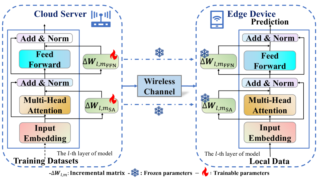
Rysunek 1: An illustrative example of remote fine-tuning of LLM over the air.

This limitation is further exacerbated in edge-cloud collaborative learning settings, where edge devices generally lack sufficient computational resources to support local fine-tuning. Consequently, model adaptation is predominantly carried out on cloud servers [7]. The updated parameters must then be transmitted to the edge over wireless channels as illustrated in Fig. 1, which are subject to limited bandwidth and fluctuating Signal-to-Noise Ratios (SNR). Meanwhile, training data collected from different sources often exhibits diverse characteristics and complexities, such as high Out-Of-Vocabulary (OOV) rates or varying lexical entropy [8], indicating the vocabulary mismatch and linguistic variability. These factors directly affect the relative importance of different layers during adaptation. More critically, most existing transmission and compression techniques are designed independently from tuning strategies [9], leading to suboptimal trade-offs between communication cost and adaptation quality.

Therefore, to overcome these limitations, efficient remote fine-tuning of Pre-trained LLMs (PLMs) [10] on the cloud and the transmission of partial, essential parameters to the edge emerge as a promising solution [11]. In other words, only a subset of layers meaningfully contribute to downstream task performance, the allocated ranks are carefully calibrated for particular PLM projection, Feed-Forward Network (FFN) [12], and output layers. Traditional heuristics, such as greedy selection or fixed allocation [6], are not equipped to handle such a dynamic, high-dimensional multi-objective problem, especially when adaptation must respond to real-time channel variations [13]. To address these challenges, we formulate communication-efficient adaptation as a sequential decision-making problem and introduce a Reinforcement Learning (RL) [14] framework to learn adaptive rank allocation policies. The proposed RL agent observes both data and channel state information [15] and dynamically adjusts rank budgets to balance model accuracy and transmission cost. However, standard RL algorithms still struggle with the underlying high-dimensional action spaces. Therefore, due to high-dimensional modeling capability, we resort to the classifier-free denoising diffusion [16, 17]. Featuring the integration of semantic-channel aware state design, diffusion-based policy generation, and a multi-objective reward formulation, our proposed framework, AirLLM, achieves balanced fine-tuning performance under bandwidth constraints. Key contributions are as follows:

• Formulating Remote Fine-Tuning as a Markov Decision Process Problem: We propose a novel formulation of remote LLM fine-tuning as a Markov Decision Process (MDP), where each decision corresponds to a layer-wise low-rank configuration under resource constraints. To support effective policy learning, we design a comprehensive RL state space incorporating wireless channel statistics (e.g., SNR), data complexity metrics (e.g., lexical entropy, OOV rate) [8], and current rank assignments. Additionally, a multi-objective reward function is constructed to balance downstream task performance with communication efficiency, enabling the RL agent to adaptively optimize fine-tuning strategies in dynamic environments.

• Hierarchical Diffusion Policy for Scalable Structured Action Generation: To address the challenge of high-dimensional decision-making in layer-wise rank allocation, we propose a hierarchical policy framework that combines a lightweight PPO-based coarse policy with a conditional DDIM [18]-based refinement module. Instead of directly predicting discrete rank configurations, the PPO [19] agent outputs a continuous latent vector representing coarse layer-wise rank guidance, which is then used to condition a DDIM sampler that progressively refines the final structured rank vector across layers. Particularly, DDIM adopts the CFG strategy to better align the denoising process with task rewards. Through training PPO and DDIM modules alternately, our approach significantly improves training stability and enables scalable action generation in large configuration spaces.

• Extensive Experimental Validation and Efficiency Gains: We conduct comprehensive experiments across multiple wireless communication scenarios and natural language understanding tasks to evaluate the effectiveness of our framework. Results demonstrate that compared to existing PEFT baselines [6], our method reduces parameter transmission costs by up to $12.5\%$ while improving task accuracy by $0.69\%$. Moreover, the proposed Diffusion-RL hybrid framework achieves over $30\%$ training efficiency gains compared to vanilla PPO [19], validating its practical applicability in real-world cloud-edge deployment settings.

This paper is organized as follows. Section II reviews related literature. Section III presents the system model and formulates the problem. Section IV details the proposed hierarchical model for fine-tuning. Section V evaluates performance via simulations. Finally, the main conclusion is drawn in Section VI.

II Related Work

II-A Parameter-Efficient Fine-Tuning for Large Language Models

The rapid advancement of LLMs has prompted an extensive investigation into PEFT methods, primarily motivated by the prohibitive cost of full-model updates in large-scale architectures. LoRA [5] pioneers this topic by replacing full fine-tuning with low-rank adaptation modules. Specifically, it approximates the update $\Delta\mathbf{W}\in\mathbb{R}^{m\times n}$ using two low-rank matrices $\mathbf{A}\in\mathbb{R}^{m\times r}$ and $\mathbf{B}\in\mathbb{R}^{r\times n}$, with $r\ll m,n$, significantly reducing trainable parameters while preserving downstream performance. However, LoRA and its early variants typically assign a uniform rank $r$ across all layers and modules, neglecting the inherent heterogeneity in importance and complexity among different components [6, 20].

To address this limitation, AdaLoRA [6] dynamically adjusts rank allocation by estimating parameter importance during training. It employs heuristic criteria derived from the SVD of parameter matrices and gradient information to guide adaptive rank adjustment. Despite these improvements, its assumption of static data distributions and system environments implies a lack of explicit mechanisms to handle dynamic and noisy wireless channels that are typical in cloud-to-edge parameter transmission [21].

II-B Adaptive Rank Allocation in Edge-Cloud Settings

Despite the progress in PEFT methods for high-performance environments, little attention has been paid to communication constraints when deploying fine-tuned parameters on resource-constrained edge devices. In edge-cloud collaborative learning, fine-tuning is commonly offloaded to cloud servers, necessitating the transmission of updated low-rank parameters over wireless channels with varying bandwidth and SNR [22, 23].

Recent studies have explored heuristic rank adaptation strategies responsive to channel conditions, such as reducing rank under low-SNR scenarios [24]. However, they typically lack principled optimization and fail to account for the interplay between data complexity and channel dynamics. To address this gap, we formulate adaptive rank allocation as a sequential decision-making problem and leverage RL to jointly optimize rank assignments based on dataset characteristics (e.g., lexical entropy, OOV rates) and real-time channel states (e.g., SNR, bandwidth) [25].

II-C Reinforcement Learning for Rank Adaptation

The integration of RL into PEFT for dynamic rank adaptation remains relatively under-explored. While conventional RL algorithms such as PPO [19] are theoretically applicable, they encounter practical challenges in large-scale Transformer-based LLMs. Specifically, assigning ranks across multiple Transformer blocks induces a high-dimensional action space, often resulting in inefficient learning and suboptimal policy performance [26, 27].

To mitigate this, diffusion policy frameworks have emerged as promising solutions by formulating policy generation as a denoising process, enabling effective modeling of complex, structured action distributions in high-dimensional spaces [28, 29]. In our approach, we adopt the DDIM [18] for its accelerated inference compared to Denoising Diffusion Probabilistic Models (DDPM) [17], while preserving expressive power for exploration. This design enables efficient rank allocation policies that balance communication cost and model accuracy under realistic edge-cloud constraints.

Tablica I: Main notations used in this paper.

Symbol	Definition
$L$	Number of Transformer layers
$d_{h}$	Hidden dimension of the model
$d_{s}$	Dimension of state
$d_{\text{MLP}}$	Hidden size of PPO policy MLP
$\mathbf{s}_{t}$	State at step $t$
$\mathbf{a}_{t}$	Action vector at $t$
$\mathbf{a}_{t}^{\text{out}}$	Coarse-grained action output by PPO
$\tilde{\mathbf{a}}_{t}$	Refined action after DDIM optimization
$R_{t}$	Reward
$\mathcal{U}(\mathbf{r}_{t})$	Task loss under rank configuration
$\eta(\mathbf{r}_{t})$	Communication cost of rank configuration
$\lambda$	Weighting between loss and communication cost
$\pi_{\theta}(\mathbf{a}\mid\mathbf{s})$	PPO policy function
$\hat{A}_{t}$	Advantage estimate
$J_{\text{CLIP}}(\theta)$	PPO clipped objective
$\mathcal{L}_{\text{PPO}}$	Total PPO loss
$\mathbf{x}_{0}$	Clean rank vector (target configuration)
$\mathbf{x}_{\tau}$	Noisy data at diffusion step $\tau$
$\hat{\mathbf{x}}_{0}$	DDIM-predicted clean rank vector
$f_{\psi}$	Noise prediction network in DDIM
$\mathcal{L}_{\text{DDIM}}$	DDIM loss combining noise + reward terms
$\kappa$	Weighting for DDIM loss terms
$T_{\text{diff}}$	Number of DDIM denoising steps
$r_{\text{max}}$	Maximum rank constraint
$\mathbf{W}_{l,m}^{(0)}$	Pre-trained weights at layer $l$, module $m$
$\mathbf{W}_{l,m}^{(t)}$	Fine-tuned weights at step $t$
$r_{l,m}^{(t)}$	Rank of module $(l,m)$ at step $t$
$\mathscr{D}$	Fine-tuning dataset
$SNR_{t}$	Signal-to-Noise Ratio
$W_{t}$	Channel bandwidth
$h_{t}$	Channel gain
$\mathbf{n}_{t}$	AWGN noise
$C_{t}$	Channel capacity
$H_{t}$	Lexical entropy of dataset at step $t$
$\rho_{t}$	OOV rate of dataset at step $t$

III System Model and Problem Formulation

III-A System Model

For convenience, we also list the main notations used in this paper in Table I.

III-A1 LLM Parameter-Efficient Fine-tuning

We consider a pre-trained Transformer-based LLM $\mathscr{M}$ composed of $L$ layers, where each layer $l\in\{1,\ldots,L\}$ contains a self-attention (SA) block and an FFN block. Without loss of generality, we exemplify the PEFT of LLM by AdaLoRA [6]. In the SA block, AdaLoRA modules (i.e., projection matrices) are inserted into the frozen projection matrices: query ($\mathbf{W}^{Q}$), key ($\mathbf{W}^{K}$), value ($\mathbf{W}^{V}$), and output ($\mathbf{W}^{O}$). In the FFN block, AdaLoRA is similarly applied to the two linear transformations $\mathbf{W}^{\text{fc1}}$ and $\mathbf{W}^{\text{fc2}}$. During fine-tuning, the original weight matrices remain frozen, while the low-rank update matrices introduced by LoRA are optimized. Mathematically, the set of LoRA-inserted modules for the $l$-th layer can be written as:

$$\mathcal{M}_{l}=\{\mathbf{W}_{l}^{Q},\mathbf{W}_{l}^{K},\mathbf{W}_{l}^{V},\mathbf{W}_{l}^{O},\mathbf{W}_{l}^{\text{fc1}},\mathbf{W}_{l}^{\text{fc2}}\}.$$ (1)

Building upon AdaLoRA, we parameterize the weight update matrix using SVD to support dynamic and fine-grained rank allocation. For each module $m$ in layer $l$ given in Eq. (1), the fine-tuned weight matrix at the $t$-th training step is expressed as:

$$\mathbf{W}^{(t)}_{l,m}=\mathbf{W}_{l,m}^{(0)}+\mathbf{P}^{(t)}_{l,m}\mathbf{\Lambda}^{(t)}_{l,m}\mathbf{Q}^{(t)}_{l,m},$$ (2)

where $\mathbf{P}^{(t)}_{l,m}\in\mathbb{R}^{d_{h}\times r^{(t)}_{l,m}}$ and $\mathbf{Q}^{(t)}_{l,m}\in\mathbb{R}^{r^{(t)}_{l,m}\times d_{h}}$ are orthogonal matrices with the hidden dimension $d_{h}$, and the rank of the diagonal singular value matrix $\mathbf{\Lambda}_{l,m}\in\mathbb{R}^{r^{(t)}_{l,m}\times r^{(t)}_{l,m}}$ with the dimension $r^{(t)}_{l,m}$. In this way, the total number of trainable parameters introduced by AdaLoRA is given by $\sum_{l=1}^{L}\sum_{m\in\mathcal{M}_{l}}r^{(t)}_{l,m}\left(2d_{h}+1\right)$.

To encourage the orthogonality of $\mathbf{P}_{l,m}$ and $\mathbf{Q}_{l,m}$, a regularization term is commonly imposed in practice, namely,

$$\mathcal{R}_{(t)}=\|{\mathbf{P}^{(t)}_{l,m}}^{\top}\mathbf{P}^{(t)}_{l,m}-\mathbf{I}\|_{F}^{2}+\|\mathbf{Q}^{(t)}_{l,m}{\mathbf{Q}^{(t)}_{l,m}}^{\top}-\mathbf{I}\|_{F}^{2},$$ (3)

where the Frobenius norm $\|\mathbf{A}\|_{F}=\sqrt{\sum_{i=1}^{m}\sum_{j=1}^{n}|a_{ij}|^{2}},$ of a matrix $\mathbf{A}\in\mathbb{R}^{m\times n}$ quantifies the element-wise distance between matrices. This regularization ensures that $\mathbf{P}_{l,m}$ and $\mathbf{Q}_{l,m}$ approach orthogonal matrices.

On the other hand, the involved fine-tuning dataset $\mathcal{D}=\{D_{1},D_{2},\dots,D_{N}\}$ can be characterized by lexical entropy and OOV rate. Specifically, for each sample $D_{n}\in\mathcal{D}$, the lexical entropy is defined as $H(D_{n})=-\sum_{w\in\mathcal{V}}\hat{p}(w)\log\hat{p}(w)$, where $\hat{p}(w)$ is the empirical probability of word $w\in D_{n}$, and $\mathcal{V}$ is the vocabulary. Meanwhile, the OOV rate is calculated by $\rho(D_{n})=\frac{|\{w\in D_{n}:w\notin\mathcal{V}\}|}{|D_{n}|}$, which measures the proportion of words in $D$ that are not in the pre-defined vocabulary $\mathcal{V}$.

III-A2 Wireless Communication Channel Model

For the remote fine-tuning of LLMs, we assume a typical cloud-edge deployment setting where the fine-tuning process is conducted on the cloud server, and the resulting low-rank parameters are transmitted to resource-constrained local edge devices. We model the wireless transmission of fine-tuned parameters from the cloud service (transmitter) to the edge device (receiver) by a slow fading Additive White Gaussian Noise (AWGN) channel. Suppose each fine-tuned parameter of a module corresponding to $\mathbf{P}^{(t)}_{l,m}$, $\mathbf{\Lambda}^{(t)}_{l,m}$ and $\mathbf{Q}^{(t)}_{l,m}$ is first compressed and then packed into a codeword $\mathbf{c}_{t}\in\mathbb{C}^{b_{t}}$ of length $b_{t}$ for transmission. The received signal at the edge is given by:

$$\mathbf{y}_{t}=h_{t}\mathbf{c}_{t}+\mathbf{n}_{t},$$ (4)

where $\mathbf{y}_{t}$ is the received signal at the local device, $h_{t}$ is the complex, slow-fading channel gain that remains constant over each block. $\mathbf{n}_{t}\sim\mathcal{CN}(0,\sigma_{t}^{2}\mathbf{I}_{b_{t}})$ represents AWGN, with $\mathbf{I}_{b_{t}}$ being the $b_{t}$-dimensional identity matrix ensuring independence of noise elements. The notation $\mathcal{CN}$ denotes the complex normal distribution, where the mean is zero and the variance is $\sigma_{t}^{2}$. The average transmit power is constrained by $\frac{1}{b_{t}}\sum_{i=1}^{b_{t}}\|\mathbf{c}_{t}(i)\|^{2}\leq P$.

Assuming perfect Channel State Information (CSI) is available at the receiver, the average achievable data rate over such a fading channel at the $t$-th step is:

$$C_{t}=\mathbb{E}_{h_{t}}\left[W_{t}\log_{2}\left(1+\text{SNR}_{t}\right)\right],$$ (5)

where $W_{t}$ is the channel bandwidth while the value of SNR is calculated with $\text{SNR}_{t}=\frac{|h_{t}|^{2}P}{\tilde{\sigma}_{t}^{2}}$.

III-B Problem Formulation

Recalling the task of transmitting fine-tuned parameters from the cloud to the edge, the number of parameters to be transmitted for each module $m$ in layer $l$, as derived from Eq. (2), is $r^{(t)}_{l,m}(2d_{h}+1)$. Accordingly, the transmission time can be calculated as

$$T^{(t)}_{l,m}=\frac{r^{(t)}_{l,m}(2d_{h}+1)\cdot b_{t}}{C_{t}},$$ (6)

where $b_{t}\equiv 32$ for FP32. In particular, the total transmission time is usually constrained by a maximum allowable latency $T_{\text{max}}$, i.e.,

$$\sum\nolimits_{l=1}^{L}\sum\nolimits_{m\in\mathcal{M}_{l}}T^{(t)}_{l,m}\leq T_{\text{max}}.$$ (7)

The constraint implicitly restricts the rank allocation across layers. Moreover, due to the limited communication capacity, there also exists a bound for the total amount of transmitted parameters, i.e., $1\leq r^{(t)}_{l,m}\leq r_{\text{max}}$, where $r_{\text{max}}$ denotes the maximum allowable rank that satisfies the communication constraint.

Given these constraints on latency and rank capacity, the pivotal challenge of our scenario lies in effectively allocating ranks across modules and layers to maximize fine-tuning performance while adhering to communication budgets. Notably, since computing task-specific metrics such as accuracy at every training step is computationally expensive, the loss value $\mathcal{U}(\mathbf{r}_{t})$ on the fine-tuning dataset $\mathcal{D}$ is adopted as a surrogate measure to monitor intermediate performance, thereby indirectly reflecting the model’s fitness under a given rank configuration $\mathbf{r}_{t}=\{r^{(t)}_{l,m}\}_{l=1,m\in\mathcal{M}_{l}}^{L}$. Meanwhile, the associated communication cost $\eta(\mathbf{r}_{t})$ is determined by the quantity of parameters transmitted from the cloud to the edge, which can be computed as:

$$\eta(\mathbf{r}_{t})=\frac{\sum_{l=1}^{L}\sum_{m\in\mathcal{M}_{l}}r_{l,m}^{(t)}(2d_{h}+1)\cdot b_{t}}{C_{t}\cdot T_{\max}}.$$ (8)

Mathematically, the optimization objective can be encapsulated as

$$\min_{\mathbf{r}} \quad\mathcal{U}(\mathbf{r}_{t})+\lambda\ \eta(\mathbf{r}_{t})$$

s.t. $$\quad\sum\limits_{l=1}^{L}\sum\limits_{m\in\mathcal{M}_{l}}\frac{r^{(t)}_{l,m}(2d_{h}+1)\cdot b_{t}}{C_{t}}\leq T_{\text{max}},$$ (9)

$$\quad 1\leq r^{(t)}_{l,m}\leq r_{\text{max}},\quad\forall l\in\{1,\dots,L\},\forall m\in\mathcal{M}_{l},$$

where $\lambda$ is a positive weighting factor that balances the significance of model performance and communication cost. In this optimization problem, reducing the communication cost $\eta(\mathbf{r}_{t})$ may lead to an increase in the loss function $\mathcal{U}(\mathbf{r}_{t})$, and vice versa [21].

Conventionally, existing PEFT methods, such as AdaLoRA, adaptively allocate rank budgets $\mathbf{r}_{t}$ across layers based on sensitivity scores or training dynamics. Nevertheless, they neglect the impact of online factors such as data-sensitive performance $\mathcal{U}(\mathbf{r}_{t})$ or wireless communication capability $C_{t}$ [6, 24]. Moreover, its local layer-wise decisions may overlook global interactions among layers and fail to satisfy strict end-to-end constraints on parameter transmission or inference latency. Hence, identifying a meticulous design of the rank parameters for each layer that satisfies all constraints while minimizing the objective function is of utmost importance.

IV Methodology

IV-A RL for Dynamic Rank Allocation

To enable dynamic rank allocation in real-world deployment scenarios, RL, particularly the PPO [19], offers a promising solution for learning adaptive policies through continuous interaction with the environment. By adopting PPO, we seek to derive a preliminary policy that effectively balances fine-tuning accuracy and communication cost under varying system conditions.

IV-A1 MDP Formulation for Rank Allocation

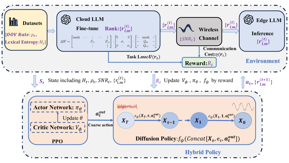
Rysunek 2: Diffusion policy framework for dynamic rank allocation in remote fine-tuning.

RL provides a dynamically adaptive decision-making paradigm for remote fine-tuning of large models, with its core advantage lying in real-time strategy optimization through environmental feedback. To enable adaptive rank configuration under real-world constraints such as wireless bandwidth and task complexity, we formulate the rank allocation as an MDP $(\mathcal{S},\mathcal{A},R)$. Such assumption allows the agent to learn context-aware policies that dynamically balance compression and performance, where the action directly corresponds to the rank configuration $\mathbf{r}_{t}$.

• State Representation: The state $\mathbf{s}_{t}=\{\mathrm{SNR}_{t},W_{t},H_{t},\rho_{t},\mathbf{r}_{t}\}\in\mathcal{S}$ is designed to comprehensively capture both the system-level constraints and task-specific complexity. Correspondingly, wireless transmission capability is implicitly acquired via $\mathrm{SNR}_{t}$ and $W_{t}$ through Eq. (5). Lexical entropy $H_{t}$ and OOV rate $\rho_{t}$ characterize the complexity of the fine-tuning dataset at time step $t$, reflecting how much expressive capacity (i.e., rank) the model may require and how many tokens that do not appear in the pretraining vocabulary. The current rank configuration $\mathbf{r}_{t}$, which represents the rank parameters for all modules in all layers, serves as the foundation upon which the next action (rank configuration) will be applied.

• Action Space: In our formulation, each Transformer layer contains $6$ LoRA-inserted projection matrices. Thus, the action vector $\mathbf{a}_{t}$ at time step $t$ (which directly defines the rank configuration) is given by $\mathbf{a}_{t}\in\{0,1,\cdots,r_{\text{max}}\}^{6L}.$ And the new rank distribution $\mathbf{r}_{t+1}=\mathbf{a}_{t}$.

• Reward Function: Consistent with the objective function in Eq. (9), the reward function can be written as

  $$R_{t}=-\mathcal{U}(\mathbf{r}_{t})-\lambda\cdot\eta(\mathbf{r}_{t}).$$ (10)

RL aims to maximize cumulative rewards through interaction with the environment. Specifically, an agent tries to learn a policy $\pi(\mathbf{a}|\mathbf{s})$, a probability distribution over actions $\mathbf{a}$ given state $\mathbf{s}$, which guides the agent’s future behaviors.

IV-A2 PPO for Coarse-Grained Policy Optimization

As noted above, we adopt PPO to train a feasible policy for dynamic rank allocation. Beforehand, we briefly present the key ingredients related to PPO. In particular, the return at time $t$ is defined as $\tilde{R}_{t}=\sum_{k=0}^{\infty}\gamma^{k}R_{t+k}$, where $\gamma\in(0,1)$ discounts future rewards. The state-value function $V_{\phi}(\mathbf{s}_{t})=\mathbb{E}_{\pi}[\tilde{R}_{t}|\mathbf{s}_{t}]$ estimates the expected return from $\mathbf{s}_{t}\in\mathbb{R}^{d_{s}}$, parameterized by a neural network with weights $\phi$. The action-value function $Q_{\pi}(\mathbf{s}_{t},\mathbf{a}_{t})=\mathbb{E}_{\pi}[\tilde{R}_{t}|\mathbf{s}_{t},\mathbf{a}_{t}]$ quantifies the return for action $\mathbf{a}_{t}$ in $\mathbf{s}_{t}$. The advantage function $\hat{A}_{t}=Q_{\pi}(\mathbf{s}_{t},\mathbf{a}_{t})-V_{\phi}(\mathbf{s}_{t})$ measures how much better or worse $\mathbf{a}_{t}$ is compared to the average action at $\mathbf{s}_{t}$, thus guiding policy improvement. Since $Q_{\pi}$ is typically unavailable, PPO estimates $\hat{A}_{t}$ via Generalized Advantage Estimation (GAE) [19], using Temporal-Difference (TD) errors:

$$\hat{A}_{t}=\sum\nolimits_{k=0}^{\infty}(\gamma\zeta)^{k}\delta_{t+k},$$ (11)

where $\delta_{t}=R_{t}+\gamma V_{\phi_{\text{old}}}(\mathbf{s}_{t+1})-V_{\phi_{\text{old}}}(\mathbf{s}_{t})$ and $V_{\phi_{\text{old}}}(\cdot)$ denotes the value function under previous parameters for stable bootstrapping. $\zeta\in[0,1]$ is the decay factor of GAE, which controls the bias-variance trade-off in advantage estimation. Eq. (11) enables efficient estimation from sampled trajectories without computing full returns.

To stabilize policy updates of the $\theta$-parametrized actor, PPO further introduces a clipped objective on top of the value function loss, which can be formulated as

$${J}_{\text{CLIP}}(\theta)=\min\left(r_{t}(\theta)\hat{A}_{t},\operatorname{clip}\big{(}r_{t}(\theta),1-\varrho,1+\varrho\big{)}\hat{A}_{t}\right),$$

$$J_{V}(\phi)=\left(V_{\phi}(\mathbf{s}_{t})-\big{(}\hat{A}_{t}+V_{\phi_{\text{old}}}(\mathbf{s}_{t})\big{)}\right)^{2},$$ (12)

$$\mathcal{L}_{\text{PPO}}=\mathbb{E}\left[{J}_{\text{CLIP}}(\theta)+J_{V}(\phi)\right],$$

where $r_{t}(\theta)=\pi_{\theta}(\mathbf{a}_{t}|\mathbf{s}_{t})/\pi_{\theta_{\text{old}}}(\mathbf{a}_{t}|\mathbf{s}_{t})$ is the probability ratio, measuring the likelihood of taking certain actions under the policy $\pi_{\theta}(\mathbf{a}_{t}|\mathbf{s}_{t})$ versus the old one $\pi_{\theta_{\text{old}}}(\mathbf{a}_{t}|\mathbf{s}_{t})$. $\operatorname{clip}(r_{t}(\theta),1-\varrho,1+\varrho)$ denotes a clipping function that limits the deviation $r_{t}(\theta)$ between successive policy updates within the range $(1-\varrho,1+\varrho)$. By minimizing the loss in Eq. (12) via gradient descent, we optimize both the policy $\pi_{\theta}$ and value function $V_{\pi}$ in PPO to achieve improved decision performance.

At each decision step, the PPO agent, implemented as a two-layer MLP, maps the current state $\mathbf{s}_{t}\in\mathbb{R}^{d_{s}}$ to a latent action prior $\mathbf{a}_{t}\in\{0,1,\ldots,r_{\max}\}^{6L}$. Given a hidden width of $d_{\text{MLP}}$, the computational complexity of single forward or backward pass is $\mathcal{O}\left(d_{\text{MLP}}\cdot\big{(}6L\cdot(r_{\max}+1)+d_{s}\big{)}+6L\cdot(r_{\max}+1)\right)$, where the first term accounts for the two-layer MLP inference that generates logits, and the second term corresponds to the element-wise softmax computation across the discrete action heads. The complexity scales linearly with the input and output dimensions.

However, PPO’s performance tends to degrade in high-dimensional discrete action spaces [30, 19]. Moreover, the gradient signal becomes increasingly sparse while the reward variations across consecutive actions remain negligible, making the estimated advantage $\hat{A}_{t}$ highly sensitive to noise and thereby resulting in unstable policy updates [31].

IV-B Diffusion Policy for High-Dimensional Actions

To mitigate the challenges of PPO in high-dimensional action space, we propose to restrict PPO to generating coarse priors $\mathbf{a}_{t}^{\text{out}}$ only, while delegating fine-grained decision-making $\mathbf{\tilde{a}}_{t}$ to a conditional diffusion model. The hierarchical coarse-to-fine strategy leverages the probabilistic noising–denoising process of diffusion models to provide a principled alternative for high-dimensional action modeling by decomposing the decision-making problem into a series of tractable local conditional distributions [16, 17]. Through the progressive denoising procedure, the hierarchical model is able to capture structural patterns across noise scales, thereby enhancing exploration capabilities and improving robustness when combined with PPO [16]. The detailed procedure is illustrated in Fig. 2.

IV-B1 Conditional Diffusion Refinement Guided by PPO Priors

Algorithm 1 The Training of Hierarchical PPO-DDIM Adaptive Rank Allocation Policy.

Input: Initialized model and hyper-parameters.
Output: Trained hierarchical policy $(\pi_{\theta},f_{\psi})$ for adaptive rank allocation.

1: for episode = $1,2,\dots$, do

2:  Observe initial state $\mathbf{s}_{0}$;

3:  for step $t=\{1,\dots,T_{\text{env}}\}$ do

4:   Generate coarse action $\mathbf{a}_{t}^{out}\sim\pi_{\theta_{\text{old}}}(\cdot|\mathbf{s}_{t})$;

5:   Initialize noise latent $\mathbf{x}_{T_{\text{diff}}}\sim\mathcal{N}(\mathbf{0},\mathbf{I})$;

6:   for $\tau=\{T_{\text{diff}}-1,\dots,0\}$ do

7:    Obtain the conditional noise prediction $\tilde{\mathbf{\bm{\epsilon}}}_{\tau,\psi}$ with Eq. (15)

8:    Predict the clean sample $\hat{\mathbf{x}}_{0}$ with Eq. (16);

9:    Refine action using DDIM procedure with Eq. (17);

10:   end for

11:   Decode refined action through Eq. (18);

12:   Deploy the rank configuration to obtain the next state $\mathbf{s}_{t+1}$;

13:   Compute reward using Eq. (10) and collect transition $\{\mathbf{s}_{t},\tilde{\mathbf{a}}_{t},R_{t},\mathbf{s}_{t+1}\}$ into batch $\mathcal{B}$;

14:  end for

15:  Compute PPO loss using samples from $\mathcal{B}$ with Eq. (12);

16:  Update PPO policy $\pi_{\theta}$ and value function $V_{\pi}$;

17:  for $\tau=\{0,\dots,T\}$ do

18:   Generate noisy sample $\mathbf{x}_{\tau}$ from clean input $\mathbf{x}_{0}$ using Eq. (13);

19:   Compute the hybrid loss according to Eq. (19);

20:   Update the parameters in noise network $f_{\psi}$ via the gradient descent.

21:  end for

22: end for

We begin by briefly introducing the forward and reverse processes of the DDPM and its deterministic variant DDIM, which achieves faster inference with similar generative quality [18]. Notably, DDIM shares the same training objective and noise schedule as DDPM, with the main distinction residing in the sampling procedure used during inference.

Forward Diffusion Process.

To enable diffusion-based training, it is essential to apply a forward noise injection process to the training data. Specifically, each clean rank configuration vector $\mathbf{x}_{0}$ is progressively corrupted by injecting Gaussian noise over $T$ discrete steps. Formally, at each timestep $\tau\in\{1,\dots,T\}$, the conditional distribution of the noisy latent variable $\mathbf{x}_{\tau}$ given the previous state $\mathbf{x}_{\tau-1}$ is defined as

$$q(\mathbf{x}_{\tau}|\mathbf{x}_{\tau-1})=\mathcal{N}\left(\mathbf{x}_{\tau};\sqrt{\alpha_{\tau}}\mathbf{x}_{\tau-1},(1-\alpha_{\tau})\mathbf{I}\right),$$ (13)

where the noise schedule parameters $\alpha_{\tau}\in(0,1)$ control the amount of noise injected, and $\mathcal{N}(\cdot;\bm{\mu},\bm{\Sigma})$ denotes a Gaussian distribution with mean $\bm{\mu}$ and covariance $\bm{\Sigma}$. By marginalizing over intermediate variables, the closed-form distribution of $\mathbf{x}_{\tau}$ conditioned on the clean sample $\mathbf{x}_{0}$ is given by

$$q(\mathbf{x}_{\tau}|\mathbf{x}_{0})=\mathcal{N}\left(\mathbf{x}_{\tau};\sqrt{\bar{\alpha}_{\tau}}\mathbf{x}_{0},(1-\bar{\alpha}_{\tau})\mathbf{I}\right).$$ (14)

Here, $\bar{\alpha}_{\tau}=\prod_{s=1}^{\tau}\alpha_{s}=\prod_{s=1}^{t}(1-\beta_{s})$ represents the cumulative product of the noise schedule up to timestep $\tau$.

Conditional Reverse Denoising Process.

The reverse diffusion process aims to iteratively denoise $\mathbf{x}_{\tau}$ back to the clean signal estimate $\mathbf{x}_{0}$. Serving as a critical component of the inference procedure, the denoising step is parameterized by a neural network $f_{\psi}(\cdot)$ that predicts the injected noise at each step. To incorporate guidance from the PPO output $\mathbf{a}_{t}^{\text{out}}$, the noise estimator is conditioned on both the noisy latent and the PPO output $\mathbf{a}_{t}^{\text{out}}$, together with the timestep embedding $\mathbf{e}_{\tau}$ that encodes the current diffusion step. Mathematically, the obtained conditional noise prediction, denoting as $\tilde{\bm{\epsilon}}_{\tau,\psi}$, can be encapsulated as

$$\tilde{\bm{\epsilon}}_{\tau,\psi}=f_{\psi}\left(\text{Concat}[\mathbf{x}_{\tau},\mathbf{e}_{\tau},\mathbf{a}_{t}^{\text{out}}]\right),$$ (15)

where $\mathbf{e}_{\tau}$ is typically implemented as a sinusoidal positional encoding to provide temporal context, and $f_{\psi}(\cdot)$ denotes the denoising network, which can be realized as a U-Net architecture [32] or a residual MLP depending on model scale and complexity.

Using the predicted noise, the posterior mean estimator of the clean signal at timestep $\tau$ is computed as

$$\mu_{\psi}(\mathbf{x}_{\tau},\tau,\mathbf{a}_{t}^{\text{out}})=\frac{1}{\sqrt{\alpha_{\tau}}}\left(\mathbf{x}_{\tau}-\frac{1-\alpha_{\tau}}{\sqrt{1-\bar{\alpha}_{\tau}}}\tilde{\bm{\epsilon}}_{\tau,\psi}\right).$$ (16)

Following the standard DDPM posterior mean, the expression can incorporate the PPO prior as a conditioning signal and generate a fine-tuned $\tilde{\mathbf{a}}_{t}$ for the rank allocation task.

Deterministic Sampling via DDIM.

For inference, we employ the DDIM sampler, which enables deterministic and efficient reconstruction of the clean action vector. Starting from an initial latent $\mathbf{x}_{T}\sim\mathcal{N}(0,\mathbf{I})$, the reverse trajectory is computed recursively, where at each step $\tau-1$, the latent vector $\mathbf{x}_{\tau-1}$ is estimated from the current value $\mathbf{x}_{\tau}$ as

$$\mathbf{x}_{\tau-1}=\sqrt{\bar{\alpha}_{\tau-1}}\hat{\mathbf{x}}_{0}+\sqrt{1-\bar{\alpha}_{\tau-1}-\sigma_{\tau}^{2}}\tilde{\bm{\epsilon}}_{\tau,\psi}+\sigma_{\tau}\bm{\epsilon},$$ (17)

where $\hat{\mathbf{x}}_{0}:=\mu_{\psi}(\mathbf{x}_{\tau},\tau,\mathbf{a}_{t}^{\text{out}})$ is the predicted clean sample, $\bm{\epsilon}\sim\mathcal{N}(0,\mathbf{I})$ is an additional noise term, and $\sigma_{\tau}\geq 0$ controls the stochasticity of the sampler with $\sigma_{\tau}=0$ yielding fully deterministic DDIM sampling.

After completing $T_{\text{diff}}\leq T$ reverse steps, the final latent $\mathbf{x}_{0}$ is transformed into the actionable discrete vector by rounding and clipping, which is formulated by

$$\tilde{\mathbf{a}}_{t}=\mathrm{clip}\left(\lfloor\mathbf{x}_{0}\rfloor,\,0,\,r_{\max}\right),$$ (18)

where $r_{\max}$ denotes the maximum allowed rank value per dimension, ensuring validity and executability of the generated action. $\lfloor\cdot\rfloor$ represents element-wise flooring to the nearest lower integer.

IV-B2 Hybrid Training Objective and Optimization.

To enhance controllability without relying on external classifiers, the training adopts the CFG strategy [33]. Specifically, the conditional diffusion model is trained to minimize a hybrid loss that combines reconstruction fidelity in noise prediction and policy effectiveness measured via task reward,

$$\mathcal{L}_{\text{DDIM}}=\mathbb{E}_{\mathbf{x}_{0},\tau,\bm{\epsilon},\mathbf{a}_{t}^{\text{out}}}\left[\left\|\tilde{\bm{\epsilon}}_{\tau,\psi}-\bm{\epsilon}\right\|_{2}^{2}\right]-\kappa\cdot\mathbb{E}_{\mathbf{s}_{t},\tilde{\mathbf{a}}_{t}}[R_{t}],$$ (19)

where the noise $\bm{\epsilon}\sim\mathcal{N}(0,\mathbf{I})$ is the ground-truth noise added at timestep $\tau$, $R_{t}$ is the reward obtained from executing the refined action $\tilde{\mathbf{a}}_{t}$ in state $\mathbf{s}_{t}$ as defined in Eq. (10), and $\kappa>0$ is a hyperparameter balancing denoising accuracy and policy reward maximization.

To maintain stability and promote complementary learning between the coarse and fine policies, we adopt an alternating training strategy that iteratively updates PPO and DDIM with shared trajectory data. Algorithm 1 summarizes the entire training and inference process for reference.

• PPO Stage: The PPO policy $\pi_{\theta}$ is trained using environment trajectories $\{(\mathbf{s}_{t},\mathbf{a}_{t},R_{t},\mathbf{s}_{t+1})\}$ to optimize the clipped surrogate loss in Eq. (12). The immediate reward $R_{t}$ is used to estimate returns $\tilde{R}_{t}$ and advantage signals $\hat{A}_{t}$, which guide updates to both the actor $\pi_{\theta}$ and critic $V_{\phi}$. The resulting output $\mathbf{a}_{t}^{\text{out}}\sim\pi_{\theta}(\cdot|\mathbf{s}_{t})$ serves as a coarse action prior.

• DDIM Stage: Holding $\pi_{\theta}$ fixed, we train the DDIM-based fine policy $f_{\psi}$ to refine $\mathbf{a}_{t}^{\text{out}}$ into fine-grained executable actions $\tilde{\mathbf{a}}_{t}$. Specifically, we sample clean actions $\mathbf{x}_{0}=\tilde{\mathbf{a}}_{t}$, perturb them to obtain noisy latents $\mathbf{x}_{\tau}$, and optimize the hybrid denoising loss , as defined in Eq. (19).

Both stages share the same replay buffer containing tuples of the form $\{\mathbf{s}_{t},\mathbf{a}_{t}^{\text{out}},\tilde{\mathbf{a}}_{t},R_{t},\mathbf{s}_{t+1}\}$. PPO explores the environment to collect trajectories and provides structural priors $\mathbf{a}_{t}^{\text{out}}$. DDIM then leverages these priors to improve action precision via denoising refinement. This closed-loop framework enables PPO and DDIM to be trained alternately but cooperatively. Based on the stability and exploration efficiency of PPO and the expressive granularity of DDIM in high-dimensional control, the entire training process ensures both robust policy optimization and fine-grained action synthesis.

IV-B3 Computational Complexity Analyses

To circumvent the inefficiency of directly generating high-dimensional discrete actions via PPO, we formulate the policy as a continuous vector generator and discard the softmax operation of PPO, resulting an $\mathcal{O}(6L\cdot(r_{\max}+1))$ saving for the computational complexity. On the other hand, the fine-grained decision-making is delegated to a conditional DDIM, which consumes the coarse latent $\mathbf{a}_{t}^{\text{out}}$ as a conditioning signal and refines a randomly initialized Gaussian latent $\mathbf{x}_{T}\sim\mathcal{N}(0,\mathbf{I})$ into a structured rank vector $\tilde{\mathbf{a}}_{t}\in\mathbb{Z}^{6L}$. The reverse denoising process unfolds over $T_{\text{diff}}$ steps, each involving a neural denoising network $f_{\psi}$ that predicts the noise residual or clean sample. Assuming $f_{\psi}$ is a two residual MLP with hidden width $d_{\text{latent}}$ and input and output dimensions of $6L$, the complexity of a single inference step is $O(L\cdot d_{\text{latent}})$. The diffusion process consists of $T_{\text{diff}}$ steps, leading to an overall inference complexity of $O(T_{\text{diff}}\cdot L\cdot d_{\text{latent}})$. When $f_{\psi}$ is a U-Net instead of MLP, it’s per-step cost scales with sequence length $L_{s}=6L$, input channel dimension $C_{\text{in}}$, and depth $L_{\text{depth}}$. For layer $i$ with $L_{i}=L_{s}/2^{i-1}$ and $C_{i}=C_{\text{in}}\cdot 2^{i-1}$, the inference complexity is: $\mathcal{O}\left(\sum_{i=1}^{L_{\text{depth}}}C_{i}^{2}\cdot L_{i}\right)=\mathcal{O}\left(C_{\text{in}}^{2}\cdot L_{s}\cdot 2^{L_{\text{depth}}}\right)$. With $T_{\text{diff}}$ steps, the total inference cost becomes $\mathcal{O}\left(T_{\text{diff}}\cdot C_{\text{in}}^{2}\cdot L_{s}\cdot 2^{L_{\text{depth}}}\right)$, highlighting its sensitivity to sequence length and depth. As $T_{\text{diff}}$ is typically small (e.g., $30-50$ steps), the overall cost remains tractable.

V Experimental Results

V-A Experimental Settings

This section presents comprehensive experimental results designed to validate the effectiveness of AirLLM for remote fine-tuning of LLM. All experiments use the SST-$2$ dataset [34] (i.e., a binary classification dataset) with the OPT-$1.3$B model [35] (a $24$-layer Transformer decoder) equipped with LoRA adapters for all linear projection layers. Wireless communication is modeled as an AWGN channel with $100$ MHz bandwidth, $1$s latency, and SNR levels ranging from $-5$ dB to $15$ dB. The total number of training steps is set to $15,000$ and we evaluate accuracy every $100$ step during the training process. If the reward value exceeds $\min[-\lambda,\,-0.5]$ and the accuracy does not improve for $5$ consecutive evaluations, we terminate training, and such an early stopping strategy applies for all models to ensure consistency [36]. Notably, this choice of reward convergence threshold is motivated by the following observation: when $\lambda$ is very small (e.g., $\lambda=0.1$ or $0.01$), the second term in Eq. (10) has a slight influence on the overall reward, and a reward value of $-0.5$ is considered sufficient to indicate convergence. In contrast, when $\lambda$ is larger (e.g., $\lambda=1$), the second term becomes more dominant, and the overall reward is lower. In this case, we consider $-\lambda$ as a sufficiently high reward value. We compare AirLLM against AdaLoRA [6] and random rank allocation baselines, and evaluate the performance in terms of binary classification accuracy. Finally, we summarize the default parameter settings in Table II.

V-B Simulation Results

V-B1 Performance Comparison

Tablica II: Default parameter settings in simulations.

Parameter	Value
MLP hidden size ($d_{\text{MLP}}$)	$256$
Discount factor ($\gamma$)	$0.95$
Decay factor of GAE ($\zeta$)	$0.95$
U-Net depth ($D$)	$6$
Kernel size ($k$)	$3$
Batch size	$32$
Learning rate of PPO	$1\times 10^{-4}$
Learning rate of DDIM	$5\times 10^{-5}$
Random seeds	$42$
Hybrid loss weight ($\kappa$)	$0.1$
Reward balance factor ($\lambda$)	$0.01$, $0.1$, $1$
Total training steps	$15,000$
DDIM inference steps ($T_{\text{diff}}$)	$30$, $50$, $100$
DDPM Training steps	$600$, $800$, $1,000$
PPO clipping factor ($\varrho$)	$0.2$
Evaluating steps	$100$
Maximum rank constraint $(r_{\text{max}})$	$8$, $16$, $32$, $64$, $128$
SNR (db)	$-5$, $0$, $5$, $10$, $15$
DDIM prediction strategy	$\bm{v}$-, $\bm{\epsilon}$-, $\bm{x_{0}}$-prediction
Noise schedule ($\beta$)	linear, cosine, scaled-linear

Tablica III: Performance comparison in terms of prediction accuracy.

Metric	AirLLM					AdaLoRA
	PPO	DDIM	PPO+DDPM	PPO+DDIM/MLP	PPO+DDIM/U-Net
Accuracy	$94.50\%$	$94.72\%$	$95.41\%$	$95.53\%$	$95.30\%$	$95.18\%$

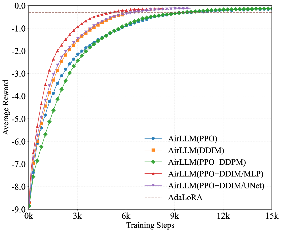
Rysunek 3: Comparison of average reward for different training methods.

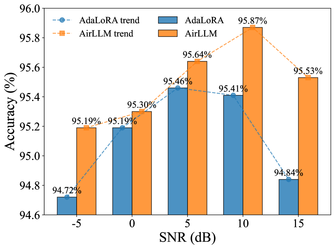
Rysunek 4: Accuracy performance evaluated under diverse SNRs.

Table III first compares the proposed AirLLM with AdaLoRA, while several variants of AirLLM with different RL algorithms are also leveraged. Notably, we also study the performance differences when using MLP and U-Net as backbones of DDIM. On the other hand, Fig. 3 gives the corresponding convergence curves. It can be observed from Table III and Fig. 3 that standalone PPO or DDIM yield the lowest accuracy. Instead, regardless of the backbone of either MLP or U-Net, the hierarchical integration achieves superior performance. Meanwhile, the integration of PPO with DDIM accelerates the convergence than that with DDPM. Finally, alongside its computational efficiency, the use of MLP also leads to better results.

In addition to efficiency and convergence speed, as shown in Fig. 4, AirLLM demonstrates superior robustness under varying channel conditions. Specifically, AirLLM achieves $0.36$%–$0.46$% higher accuracy compared to AdaLoRA, consistently adapting its rank configurations to dynamic bandwidth availability. Furthermore, benchmarking experiments in Table IV comprehensively evaluate AirLLM against AdaLoRA under varying rank budgets (i.e., $r_{\text{max}}$). The results demonstrate that AirLLM consistently outperforms the baseline across all settings. Particularly, it achieves a notable higher accuracy at $r_{\text{max}}=64$ while simultaneously reducing transmitted parameters by $12.5\%$. These results collectively validate the effectiveness of AirLLM: by unifying PPO’s stability and DDIM’s high-dimensional modeling, the framework meets the dual objectives of high accuracy and communication efficiency in remote fine-tuning scenarios, confirming the theoretical motivation proposed in Section IV.

Tablica IV: Comparison in terms of accuracy and transmitted parameters.

Rank ($r_{\text{max}}$)	Accuracy (%)		Transmitted Parameters
	AdaLoRA	AirLLM	AdaLoRA	AirLLM
$8$	$95.18$	$\mathbf{95.64}\uparrow$	$4,718,592$	$4,235,648\downarrow$
$16$	$94.72$	$\mathbf{95.30}\uparrow$	$9,437,184$	$8,471,296\downarrow$
$32$	$95.41$	$\mathbf{95.87}\uparrow$	$18,874,368$	$16,942,592\downarrow$
$64$	$94.84$	$\mathbf{95.53}\uparrow$	$32,399,048$	$28,234,160\downarrow$
$128$	$94.72$	$\mathbf{95.19}\uparrow$	$63,870,464$	$56,664,832\downarrow$

V-B2 Performance Sensitivity Studies

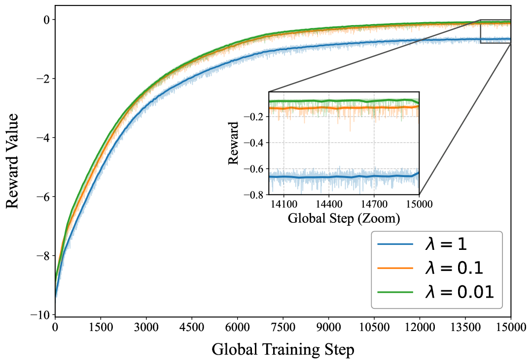
Rysunek 5: Impact of reward coefficient $\lambda$.

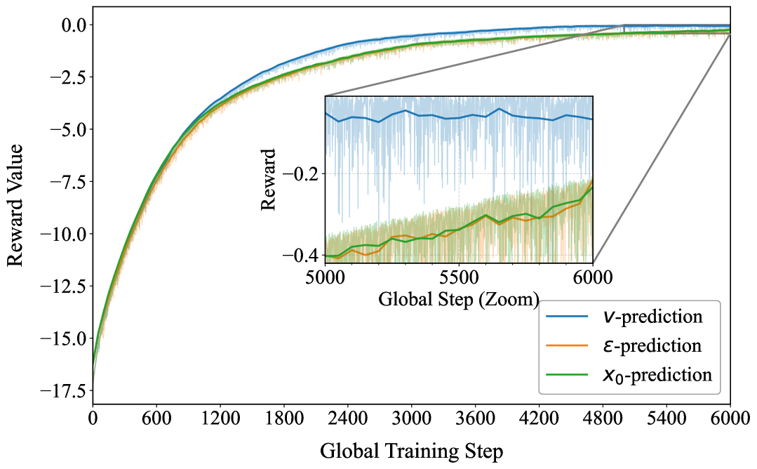
Rysunek 6: The training reward of policy with different DDIM prediction strategies.

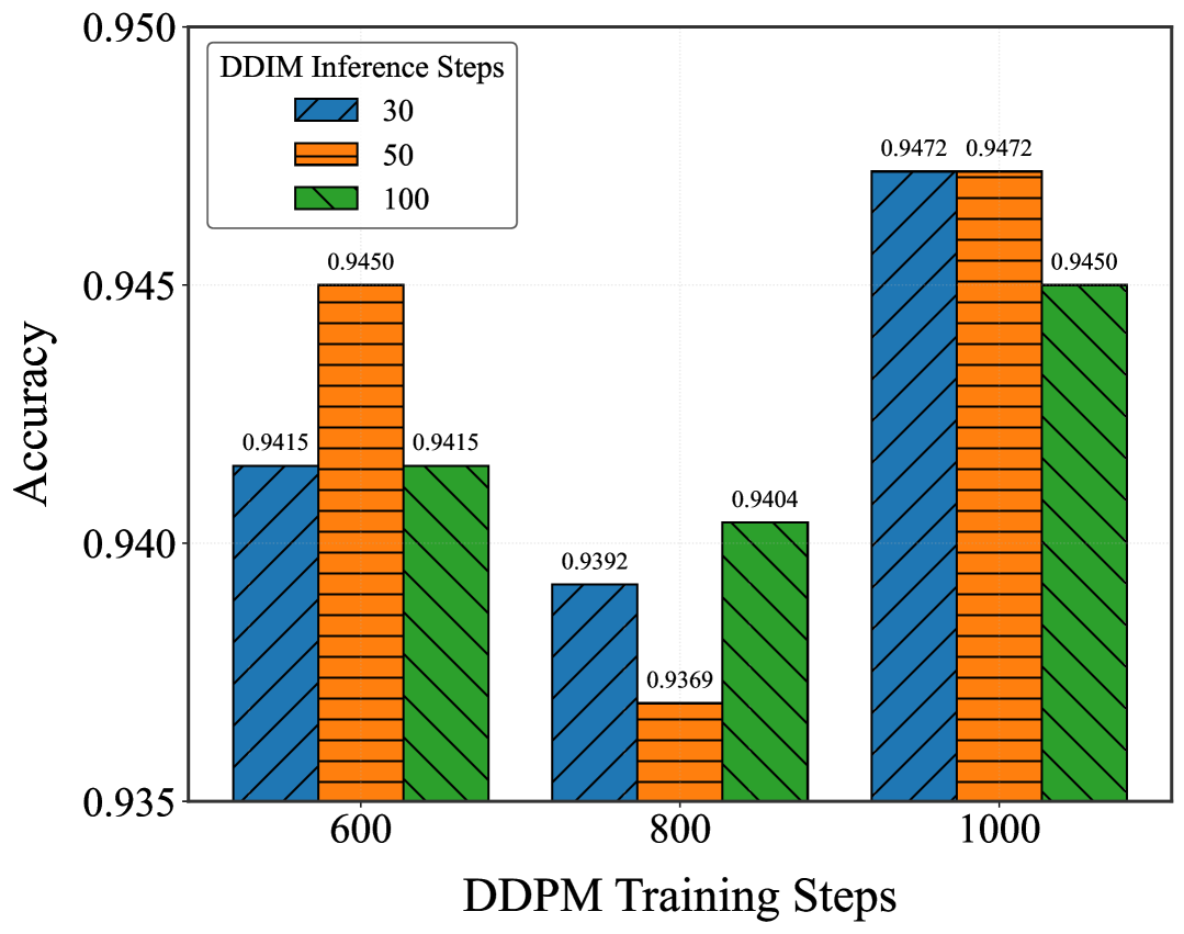
Rysunek 7: Accuracy performance evaluated under varying DDPM training steps and DDIM Inference steps.

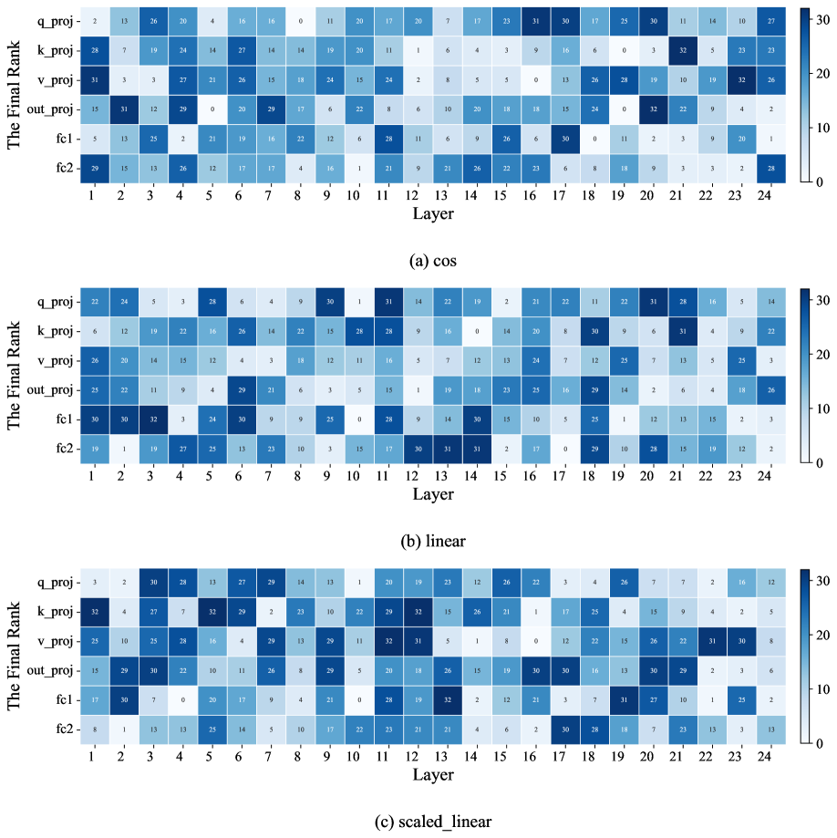
Rysunek 8: Rank distribution under different $\beta$ schedules.

Tablica V: Classification accuracy under different settings.

(a) Accuracy for Different $\lambda$ Values
	$\lambda=1$	$\lambda=0.1$	$\lambda=0.01$
Accuracy	95.07%	95.41%	94.95%
(b) Accuracy for Different Prediction Types
	$\bm{v}$-prediction	$\bm{\epsilon}$-prediction	$\bm{x_{0}}$-prediction
Accuracy	95.30%	95.30%	95.07%

Next, we examine the impact of the reward balancing coefficient $\lambda$, which as defined in Eq. (10), regulates the trade-off between task accuracy and communication cost. Fig. 5 shows $\lambda=0.1$ or $\lambda=0.01$ achieves superior, competitive balance, namely higher reward values with faster convergence. Table V(a) further confirms the superiority of $\lambda=0.1$ in classification accuracy. On the contrary, a smaller $\lambda$ compromises the balance.

We further consider different DDIM prediction strategies [37], each representing a distinct modeling choice. The $\bm{\epsilon}$-prediction estimates residual noise, directly aligning with the probabilistic structure of the diffusion process for stable and accurate reconstruction. The $\bm{v}$-prediction models a velocity-like intermediate variable defined as $\bm{v}=\sqrt{\bar{\alpha}_{t}}\,\bm{\epsilon}-\sqrt{1-\bar{\alpha}_{t}}\,\bm{x}_{0},$ which combines both noise and clean signal components, offering a balanced view of the denoising dynamics. The $\bm{x_{0}}$-prediction directly targets the clean data, but this approach is more sensitive to boundary effects in high-dimensional spaces, leading to larger convergence fluctuations. Table V(b) shows that both $\bm{\epsilon}$-prediction and $\bm{v}$-prediction achieve high accuracy, outperforming $\bm{x_{0}}$-prediction at a lower value. Similarly, Fig 6 shows $\bm{v}$-prediction obtain higher reward, however, the other two prediction methods also gain a high reward. These results further confirm the advantage of residual noise or intermediate variable modeling over direct data recovery for dynamic rank allocation in diffusion-based policies.

Tablica VI: Total inference time (s) for different inference steps.

DDPM Training Steps	DDIM Inference Steps	Total Time (s)
$600$	$30$	$907$
$600$	$50$	$1,037$
$600$	$100$	$1,101$

Fig. 7 presents the impact of different training and inference steps. It can be observed that the configuration with $1,000$ steps for training and $50$ steps for inference achieves $95.30\%$ accuracy. As shown in Table VI, under the same number of DDPM training steps, we set different DDIM inference steps to complete the full training of $1,000$ episodes. The comparison indicates that the training time increases significantly as the number of inference steps grows, demonstrating a direct impact of inference steps on the overall training duration. Sufficient training enables the diffusion model to learn noise patterns, while excessive inference steps ($T_{\text{diff}}\geq 50$) increase latency by $40\%$ with negligible gains.

The $\beta$ schedule in Eq. (16) shapes the rank distribution by controlling noise degradation. Fig. 8 shows that the scaled-linear schedule outperforms alternatives by assigning higher average ranks to lower layers, which is consistent with the characteristics of our decoder-only model that relies on strong local representations in early layers [38]. In addition, the schedule allocates larger ranks to critical modules such as $\mathbf{W}^{O}$ and $\mathbf{W}^{\text{fc1}}$, aligning with the findings of AdaLoRA [6] on the importance of these components for preserving task performance. This matches the cumulative SNR expression $\bar{\alpha}_{t}=\prod(1-\beta_{s})$, where slower noise degradation in lower layers preserves essential rank information, while faster degradation in higher layers effectively prunes redundant parameters—meeting OPT-1.3B’s architectural demands for communication-efficient adaptation.

VI Conclusion

This paper has presented AirLLM, a novel framework for communication-efficient remote fine-tuning of LLMs. Compared to the static rank allocation in AdaLoRA, AirLLM has integrated PPO with DDIM to dynamically optimize allocated ranks, further affecting the fine-tuned SVD matrices for over-the-air transmission. The PPO and DDIM components are alternately trained in a decoupled manner, where DDIM adopts the CFG strategy to improve controllability and reward alignment. By embedding channel conditions (SNR, bandwidth) and dataset characteristics (lexical entropy, out-of-vocabulary rate) into an RL state space, AirLLM has adaptively balanced model performance and parameter transmission efficiency. Particularly, AirLLM has achieved up to a $0.69$% accuracy improvement over AdaLoRA while reducing transmitted parameters by $12.5$% at $r_{\text{max}}=64$. The convergence speed has been accelerated by $20\textendash 30$% via DDIM sampling, showcasing the framework’s effectiveness in high-dimensional action spaces. These findings have validated AirLLM’s superior efficiency in remote fine-tuning of LLMs. Future work may explore multi-agent collaboration and adaptive noise scheduling to enhance scalability and robustness in extreme channel conditions.

- [1] OpenAI, “GPT-4 technical report,” OpenAI, Tech. Rep. arXiv:2303.08774, 2023, arXiv preprint arXiv:2303.08774. [Online]. Available: https://arxiv.org/abs/2303.08774
- [2] DeepSeek-AI, “Deepseek-v2 technical report,” DeepSeek-AI, Tech. Rep. arXiv:2405.04434, 2024, arXiv preprint arXiv:2405.04434. [Online]. Available: https://arxiv.org/abs/2405.04434
- [3] W. X. Zhao, K. Zhou, J. Li, T. Tang, X. Wang, Y. Hou, Y. Min, B. Zhang, J. Zhang, Z. Dong, Y. Du, C. Yang, Y. Chen, Z. Chen, J. Jiang, R. Ren, Y. Li, X. Tang, Z. Liu, P. Liu, J.-Y. Nie, and J.-R. Wen, “A survey of large language models,” arXiv preprint arXiv:2303.18223, 2023. [Online]. Available: https://arxiv.org/abs/2303.18223
- [4] V. Lialin, V. Deshpande, and A. Rumshisky, “Scaling down to scale up: A guide to parameter-efficient fine-tuning,” arXiv preprint arXiv:2303.15647, 2023.
- [5] E. J. Hu, Y. Shen, P. Wallis, Z. Allen-Zhu, Y. Li, S. Wang, L. Wang, and W. Chen, “LoRA: Low-Rank adaptation of large language models,” in Proc. ICLR, Virtual Edition, Apr. 2022.
- [6] Q. Zhang, Z. Liu, J. Fu, H. Dong, X. Han, P. Zhang, Y. Sun, H. Tian, H. Wu, and H. Wang, “AdaLoRA: Adaptive budget allocation for parameter-efficient fine-tuning,” in Proc. ICLR, Kigali, Rwanda, May 2023.
- [7] A. R. Hummaida, N. W. Paton, and R. Sakellariou, “Adaptation in cloud resource configuration: a survey,” J. Cloud Comput., vol. 5, no. 1, p. 7, 2016.
- [8] B. Xu, L. Zhang, Z. Mao, Q. Wang, H. Xie, and Y. Zhang, “Curriculum learning for natural language understanding,” in Proc. ACL, Virtual Edition, Jul. 2020.
- [9] S. Han, H. Mao, and W. J. Dally, “Deep compression: Compressing deep neural networks with pruning, trained quantization and huffman coding,” in Proc. ICLR, San Juan, Puerto Rico, May 2016.
- [10] X. Qiu, T. Sun, Y. Xu, Y. Shao, N. Dai, and X. Huang, “Pre-trained models for natural language processing: A survey,” Sci. China Technol. Sci., vol. 63, no. 10, pp. 1872–1897, 2020.
- [11] H. Yang, P. F. Smulders, and M. H. Herben, “Channel characteristics and transmission performance for various channel configurations at 60 GHz,” Eurasip J. Wirel. Commun. Netw., vol. 2007, no. 1, p. 019613, 2007.
- [12] G. Bebis and M. Georgiopoulos, “Feed-forward neural networks,” IEEE Potentials, vol. 13, no. 4, pp. 27–31, 1994.
- [13] C. U. Bas, R. Wang, S. Sangodoyin, D. Psychoudakis, T. Henige, R. Monroe, J. Park, C. J. Zhang, and A. F. Molisch, “Real-time millimeter-wave MIMO channel sounder for dynamic directional measurements,” IEEE Trans. Veh. Technol., vol. 68, no. 9, pp. 8775–8789, 2019.
- [14] C. Szepesvári, Algorithms for reinforcement learning. Springer nature, 2022.
- [15] Z. Qi, Y. Feng, and Z. Qin, “Adaptive sampling and joint semantic-channel coding under dynamic channel environment,” arXiv preprint arXiv:2502.07236, 2025.
- [16] A. Z. Ren, T. Yu, C. Finn, and S. Levine, “Diffusion policy policy optimization,” in Proc. ICLR, Singapore, Apr 2025.
- [17] J. Ho, A. Jain, and P. Abbeel, “Denoising diffusion probabilistic models,” in Proc. NeurIPS, Virtual Edition, Dec. 2020.
- [18] J. Song, C. Meng, and S. Ermon, “Denoising diffusion implicit models,” in Proc. ICLR, Vienna, Austria, May 2021.
- [19] J. Schulman, F. Wolski, P. Dhariwal, A. Radford, and O. Klimov, “Proximal policy optimization algorithms,” arXiv preprint arXiv:1707.06347, 2017.
- [20] C. Clarke, Y. Heng, L. Tang, and J. Mars, “PEFT-U: Parameter-efficient fine-tuning for user personalization,” arXiv preprint arXiv:2407.18078, 2024.
- [21] L. Zhang, J. Peng, J. Zheng, and M. Xiao, “Intelligent cloud-edge collaborations assisted energy-efficient power control in heterogeneous networks,” IEEE Trans. Wirel. Commun., vol. 22, no. 11, pp. 7743–7755, 2023.
- [22] T. S. Rappaport, Wireless Communications: Principles and Practice. Pearson Education India, 2020.
- [23] A. Goldsmith, Wireless Communications. Cambridge University Press, 2005.
- [24] B. Wu, R. Zhu, Z. Zhang, P. Sun, X. Liu, and X. Jin, “dLoRA: Dynamically orchestrating requests and adapters for LoRA/LLM serving,” in Proc. OSDI, Santa Clara, CA, USA, Jul. 2024.
- [25] R. S. Sutton and A. G. Barto, Reinforcement Learning: An Introduction. MIT Press, 2018.
- [26] Y. Peng, J. Zeng, Y. Hu, Q. Fang, and Q. Yin, “Reinforcement learning from suboptimal demonstrations based on reward relabeling,” Expert Syst. Appl., vol. 255, p. 124580, 2024.
- [27] N. Heess, H. Soyer, A. Saxena, T. Joachims, T. Degris, P. M. Pilarski, A. J. Ballard, D. Wierstra, and J. Peters, “Learning continuous control policies by stochastic value gradients,” in Proc. NeurIPS, Montreal, Quebec, Canada, Dec. 2015.
- [28] T. Haarnoja, K. Hartikainen, P. Abbeel, and S. Levine, “Latent space policies for hierarchical reinforcement learning,” in Proc. ICML. PMLR, 2018, pp. 1851–1860.
- [29] D. N. Lee and M. R. Kosorok, “Off-policy reinforcement learning with high dimensional reward,” arXiv preprint arXiv:2408.07660, 2024.
- [30] P. Henderson, R. Islam, P. Bachman, J. Pineau, D. Precup, and D. Meger, “Deep reinforcement learning that matters,” in Proc. AAAI, New Orleans, LA, USA, Feb. 2018.
- [31] M. Andrychowicz, A. Raichuk, P. Stańczyk, M. Orlowski, L. Espeholt, R. Marinier, M. Zięba, J. Kay, Y. Tassa, N. Heess et al., “What matters in on-policy reinforcement learning? A large-scale empirical study,” in Proc. ICLR, Vienna, Austria, May 2021.
- [32] R. Rombach, A. Blattmann, D. Lorenz, P. Esser, and B. Ommer, “High-resolution image synthesis with latent diffusion models,” in Proc. CVPR, New Orleans, LA, USA, Jun. 2022.
- [33] J. Ho and T. Salimans, “Classifier-free diffusion guidance,” in Proc. NeurIPS, Virtual Edition, Dec. 2021.
- [34] R. Socher, A. Perelygin, J. Wu, J. Chuang, C. D. Manning, A. Y. Ng, and C. Potts, “Recursive deep models for semantic compositionality over a sentiment treebank,” in Proc. EMNLP, Seattle, WA, USA, Oct. 2013.
- [35] S. Zhang, S. Roller, N. Goyal, M. Artetxe, M. Chen, S. Chen, G. Dewan, M. Diab, J. Dodge, X. L. Maestre, X. V. Lin, T. Mihaylov, M. Ott, S. Shleifer, K. Shuster, D. Simig, P. S. Koura, A. Singh, H. Schwenk, and L. Zettlemoyer, “OPT: Open pre-trained transformer language models,” arXiv preprint arXiv:2205.01068, 2022.
- [36] G. Raskutti, M. J. Wainwright, and B. Yu, “Early stopping and non-parametric regression: an optimal data-dependent stopping rule,” J. Mach. Learn. Res., vol. 15, no. 1, p. 335–366, Jan. 2014.
- [37] C. Chi, S. Feng, Y. Du, Z. Xu, E. Cousineau, B. Burchfiel, and S. Song, “Diffusion Policy: Visuomotor policy learning via action diffusion,” in Proc. RSS, Daegu, Republic of Korea, Jul. 2023.
- [38] X. Zhang, B. Yu, H. Yu, Y. Lv, T. Liu, F. Huang, H. Xu, and Y. Li, “Wider and deeper LLM networks are fairer LLM evaluators,” arXiv preprint arXiv:2308.01862, 2023.