Recursive Bound-Constrained AdaGrad with Applications
to Multilevel and Domain Decomposition Minimization

Abstract

Two OFFO (Objective-Function Free Optimization) noise tolerant algorithms are presented that handle bound constraints, inexact gradients and use second-order information when available. The first is a multi-level method exploiting a hierarchical description of the problem and the second is a domain-decomposition method covering the standard addditive Schwarz decompositions. Both are generalizations of the first-order AdaGrad algorithm for unconstrained optimization. Because these algorithms share a common theoretical framework, a single convergence/complexity theory is provided which covers them both. Its main result is that, with high probability, both methods need at most ${\pazocal{O}}(\epsilon^{-2})$ iterations and noisy gradient evaluations to compute an $\epsilon$-approximate first-order critical point of the bound-constrained problem. Extensive numerical experiments are discussed on applications ranging from PDE-based problems to deep neural network training, illustrating their remarkable computational efficiency.

Keywords: nonlinear optimization, multilevel methods, domain decomposition, noisy gradients, objective-function-free optimization (OFFO), AdaGrad, machine learning, complexity, bound constraints.

1 Introduction

Consider the problem

$$\min_{x\in{\pazocal{F}}}f_{r}(x),\;\;\mbox{ where }\;\;{\pazocal{F}}=\big{\{}x\in\hbox{I\thinspace R}^{n_{r}}\mid l_{r,i}\leq x_{i}\leq u_{r,i}\;\;\mbox{for}\;\;i\in\{1,\ldots,n_{r}\}\big{\}}$$ (1)

and where $f_{r}$ is a smooth possibly nonconvex and noisy function from $\hbox{I\thinspace R}^{n}$ into IR. Problems of this type frequently arise in diverse scientific applications, e.g., contact or fracture mechanics [53, 60]. Another prominent application area involves inverse problems and PDE-constrained optimization (under uncertainty) [22], where the reduced functional is often subject to bounds ensuring the physical feasibility. Moreover, in recent years, bound-constrained minimization problems have also emerged in machine learning due to the incorporation of prior knowledge into the design of machine learning models. For instance, features or weights [62] are often restricted to specific ranges to prevent overfitting. Moreover, in scientific machine learning, bounds are frequently applied to reflect real-world limits and maintain physical interpretability [64]. Although these application areas are fairly diverse, the arising minimization problems face a common challenge: solving the underlying minimization problems is computationally demanding due to the typically large dimensionality $n\in\mathbb{N}$, severe ill-conditioning and the presence of both noise and bounds.

Noise in the objective function may be caused by a number of factors (such as data sampling or variable precision computations, for instance), but we subsume all these cases here by considering that noise affects the objective function randomly. Various strategies have been proposed to handle this situation in the standard linesearch, trust-region or adaptive regularization settings (see [18, 19, 9, 11, 39, 8, 10, 7], to cite only a few), but one of the most successful is the Objective-Function-Free-Optimization (OFFO) technique. Taking into account that optimization of noisy functions require more accuracy on the objective function value than on its derivatives, OFFO algorithms bypass this difficulty by never computing such values, yielding substantially improved reliability in noisy situations. Popularized in (unconstrained) machine learning, where noise is typically caused by sampling, OFFO algorithms such as stochastic gradient descent (SGD) [73], AdaGrad [26] or Adam [50] (among many others) have had a significant impact on numerical optimization.

In this paper, we propose ML-ADAGB2 and DD-ADAGB2, two new OFFO variants of ADAGB2  in order to alleviate the computational challenge mentioned above. Both variants allow the use of second-order information, should it be available, bounds on the variables and stochastic noise on the gradients, while exploiting structure frequently present in problems of the form (1).

A first example of such structure occurs when (1) arises from the discretization of an infinite-dimensional problem, in which case cheap surrogates of the objective function can be constructed by exploiting discretizations with lower resolutions. Multilevel methods are well known to take advantage of such structure. They have been originally proposed to solve discretized elliptic partial differential equations (PDEs) [14], for which they have been show to exhibit optimal complexity and convergence rate independent of the problem size. Since then, the multilevel approaches have been successfully extended to solve non-convex minimization problems, using multilevel line-search (MG-OPT) [67], multilevel trust-region (RMTR) [38] or multilevel higher- order regularization strategies (M-ARC) [17].

Extending multilevel methods to handle bound-constraints is challenging, as the lower levels are often unable to resolve fine-level constraints sufficiently well, especially when the constraints are oscillatory [58]. Initial attempts to incorporate constraints into the multilevel framework involved solving linear complementarity problems; see, for instance, [65, 13, 45, 30]. These methods employed various constraint projection rules to construct lower-level bounds so that prolongated lower-level corrections would not violate the finest level bounds. However, these projection rules tend to be overly restrictive, resulting in multilevel methods that converge significantly slower than standard linear multigrid. To improve convergence speed, Kornhuber proposed a truncated monotone multigrid method [57] which employs a truncated basis approach and recovers the convergence rate of the unconstrained multigrid once the exact active-set is detected [47, 57].

In the context of nonlinear optimization, only a few multilevel algorithms for bound constrained problems exist. For instance, Vallejos proposed a gradient projection-based multilevel method [76] for solving bilinear elliptic optimal control problems. In [51], two multilevel linesearch methods were introduced for convex optimization problems, incorporating the constraint projection rules from [45] and an active-set approach from [57]. For non-convex optimization problems, Youett et al. proposed a filter trust-region algorithm [77] that employs an active-set multigrid method [57] to solve the resulting linearized problems. Additionally, Gratton et al. introduced a variant of the RMTR method [37], utilizing constraint projection rules from [30]. This approach was later enhances in [54] by employing the Kornhuber’s truncated basis approach. Our new ML-ADAGB2 algorithm follows similar ideas, but in the noise tolerant OFFO context.

A second important example of problem structure, again typically arising in problems associated with PDEs, involves cases where the problem’s variables pertain to subdomains on which the underlying problem can be solved at a reasonable cost. This naturally leads to a class of methods known as domain-decomposition methods. As with multilevel methods, domain-decomposition methods were originally developed for solving elliptic PDEs, giving rise to techniques such as the (restricted) additive Schwarz methods [24, 16]. In the context of nonlinear problems, much of the focus has been on improving the convergence of Newton’s method. In particular, Cai et al. proposed an additively preconditioned inexact Newton method, known as ASPIN [15]. The core idea behind this approach is to rebalance the nonlinearities by solving restricted nonlinear systems on subdomains. Since then, numerous variants of additive preconditioners for Newton’s method have appeared in the literature, e.g., RASPEN [23] and SRASPEN [21].

Within the framework of nonlinear optimization, the literature is comparatively sparse, but several inherently parallel globalization strategies have been developed. These include parallel variable and gradient distribution techniques [27, 66], additively preconditioned line search methods [70], and domain-decomposition-based trust-region approaches [41, 42, 40]. More recently, several efforts have explored the use of nonlinear domain decomposition methods for machine learning applications, such as additively preconditioned L-BFGS [52] or trust-region method [75]. While these approaches show promise for improving training efficiency and increasing model accuracy, to the best of our knowledge, none of the existing domain decomposition algorithms have yet been designed to be tolerant to (subsampling) noise, as required in practical applications.

Extending domain-decomposition methods to handle bound constraints is generally simpler than in the case of multilevel methods, since constraints may often be easily restricted to each subdomain. To this aim, Badia et al. developed the variants of additive Schwarz for linear variational inequality [4, 3, 2]. In [59], a nonlinear restricted additive Schwarz preconditioner was introduced to precondition a Newton-SQP algorithm. More recently, Park proposed the additive Schwarz framework for solving the convex optimization problems based on the (accelerated) gradient methods [68, 69]. In the context of non-convex optimization, trust-region-based domain decomposition algorithms that enforce the trust-region constraint in the infinity norm naturally facilitate the incorporation of bound constraints; see, for example, [42].

As noted in [40, 36], domain decomposition methods share strong conceptual similarities with multilevel approaches. Indeed, combining multilevel and domain decomposition methods is often essential in order to design highly parallel and algorithmically scalable algorithms. One of the key objectives of this work is to leverage this connection to develop a new domain decomposition method, DD-ADAGB2, which—like ML-ADAGB2—operates without requiring function values, supports bound constraints, and remains robust under stochastic gradient approximations.

We summarize our contributions as follows.

1. We propose the OFFO multilevel ML-ADAGB2 algorithm for problem exhibiting a hierarchical description, whose distinguishing features are its capacity to handle bound constraints and its good reliability in the face of noise (due to its OFFO nature and its tolerance to random noise in the gradients). It is also capable of exploiting second-order information, should it be accessible at reasonable cost.

2. We then apply the concepts developed for the multilevel case to the context of domain-decomposition and propose the more specialized DD-ADAGB2 algorithm with the same features.

These contributions build upon the analysis of [6] for the single level stochastic OFFO case, the techniques presented in [38, 37] for multilevel deterministic non-OFFO and in [35] for unconstrained multilevel OFFO, and on the discussion of the domain-decomposition framework in [40, Section 5].

After this introduction, Section 2 describes hierarchical problems in more detail and proposes the ML-ADAGB2 OFFO algorithm. Its convergence and computational complexity is then analyzed in Section 3, while Section 4 describes its extension to the domain-decomposition context. Numerical experiments presented in Section 5 illustrate the efficiency, scope and versatility of the proposed methods. Some conclusions are finally discussed in Section 6.

2 An OFFO multilevel algorithm for hierarchical problems

Given problem (1), we assume that there exists a hierarchy of spaces $\{\hbox{I\thinspace R}^{n_{\ell}}\}_{\ell=0}^{r}$ where (possibly local or simplified) version of the problem can be described. We refer to these spaces as levels, from the top one (indexed by $\ell=r)$ to the bottom one (indexed by $\ell=0$). Our algorithm is iterative and generates iterates $x_{\ell,k}\in\hbox{I\thinspace R}^{n_{\ell}}$, where the first subscripts denotes the level and the second the iteration within that level. At the top level, the task consists in minimizing $f_{r}$, the problem’s objective function. For each feasible iterate $x_{r,k}$ it is possible to construct, at level $r-1$, a model $f_{r-1}$ of $f_{r}$, using local information such has $g_{r,k}$ (an approximation of $\nabla_{x}f_{r}(x_{r,k})$) and the restriction operator $R_{r}$. The bounds on the variables, if present, can also be transferred to level $r-1$ using the $R_{r}$, yielding a feasible set at level $r-1$, denoted ${\pazocal{F}}_{r-1}$. The minimization may then be pursued at level $r-1$, descending on $f_{r-1}$ and generating iterates ${x_{r-1,0},x_{r-1,1},\ldots\ \text{in}\ {\pazocal{F}}_{r-1}}$. Again, at each of these iterates, it is possible to construct, at level $r-2$, a model $f_{r-2}$ of $f_{r-1}$ and a feasible set ${\pazocal{F}}_{r-2}$, and so on until level $l=0$ is reached, where the construction of a lower level approximation of $f_{0}$ is either impossible or too coarse. Once an iteration at level $\ell$ is concluded (either because an approximate critical point is reached or because the maximum number of iterations is exceeded), the final iterate $x_{\ell,*}$ is prolongated to level $\ell+1$ using the operator $P_{\ell+1}$.

As we have already mentioned, the iterates at level $\ell$ are denoted by $x_{\ell,k}$ for values of $k$ increasing from 0. Note that this is slightly ambiguous since iterates generated at level $\ell-1$ from different iterates at level $\ell$ share the same indices, but a fully explicit notation is too cumbersome, and no confusion arises in our development. The components of $x_{\ell,k}$ are denoted $x_{\ell,k,i}$, for ${i\in\{1,\ldots,n_{\ell}\}}$. We also denote

$$G_{\ell,k}=\nabla_{x}^{1}f_{\ell}(x_{\ell,k}),\;\;\;\;g_{\ell,k}\approx\nabla_{x}^{1}f_{\ell}(x_{\ell,k}),\;\;\mbox{ and }\;\;H_{\ell,k}\approx\nabla_{x}^{2}f_{\ell}(x_{\ell,k}).$$

If the bounds on the variables at level $\ell$ are $l_{\ell}$ and $u_{\ell}$, we have that ${\pazocal{F}}_{\ell}=\prod_{i=1}^{n_{\ell}}[l_{\ell,i},u_{\ell,i}]$. In what follows, we assume that, for each $\ell$, $P_{\ell}$ and $R_{\ell}$ have non-negative entries. We define the vector of row-sums. $\sigma_{\ell}$, as given component-wise by

$$\sigma_{\ell,i}=\sum_{j\in\{1,\ldots,n_{\ell-1}\}|P_{\ell,i,j}>0}P_{\ell,i,j}=\sum_{j=1}^{n_{\ell-1}}P_{\ell,i,j}\;\;\;\;(i\in\{1,\ldots,n_{\ell}\}).$$ (2)

When the $j$-th column is zero, we may choose $\sigma_{\ell,j}\geq 0$ arbitrarily and we also define the maximum and minimum on the empty set $\{i\in\{1,\ldots,n_{\ell}\}|\mid P_{\ell,i,j}>0\}$ to be are arbitrary with the latter not exceeding the former. Using these conventions, we may now describe the ML-ADAGB2 algorithm.

Algorithm 2.1: ML-ADAGB2
Initialization: The bounds $l$ and $u$, the starting point $x_{r,0}$, the hierarchy $\{f_{\ell},\sigma_{\ell},m_{\ell}\}_{\ell=0}^{r}$, $\{P_{\ell},R_{\ell}\}_{\ell=0}^{r-1}$, and the constants $\kappa_{s},\kappa_{\mbox{\tiny 2nd}}\geq 1$ and $\kappa_{\mbox{\tiny 1st}},\kappa_{\mbox{\tiny gs}},\varsigma\in(0,1]$ are given. Top level optimization: return ML-ADAGB2-r$(r,P_{\pazocal{F}}(x_{r,0}),l,u,\varsigma^{2},0,\infty,m_{r})$

Algorithm 2.2: $x_{\ell,*}=$ ML-ADAGB2-r ($\ell,x_{\ell,0},l_{\ell},u_{\ell},w_{\ell,-1},\theta_{1,\ell},\theta_{2,\ell},m_{\ell}$)
Step 0: Initialization: Set $k=0$. Step 1: Start iteration: Compute $g_{\ell,k}$ as an approximation of $G_{\ell,k}$, $$d_{\ell,k}\stackrel{{\scriptstyle\rm def}}{{=}}P_{{\pazocal{F}}_{\ell}}(x_{\ell,k}-g_{\ell,k})-x_{\ell,k},$$ (3) $$w_{\ell,k,i}=\sqrt{w_{\ell,k-1,i}^{2}+d_{\ell,k,i}^{2}}\;\;\mbox{and}\;\;\Delta_{\ell,k,i}=\frac{|d_{\ell,k,i}|}{w_{\ell,k,i}},\;\;\mbox{ for }\;\;i\in\{1,\ldots,n_{\ell}\}.$$ (4) If $\ell<r$ and $k=0$, readjust $$w_{\ell,0}\leftarrow\max\left[1,\frac{\|\Delta_{\ell,0}\|}{\theta_{2,\ell}}\right]\,w_{\ell,0}\;\;\mbox{ and }\;\;\Delta_{\ell,0}\leftarrow\min\left[1,\frac{\theta_{2,\ell}}{\|\Delta_{\ell,0}\|}\right]\,\Delta_{\ell,0}$$ (5) and return $x_{\ell,*}=x_{\ell,0}$ if $$|d_{\ell,0}^{T}\Delta_{\ell,0}|<\theta_{1,\ell}.$$ (6) Otherwise, set $${\pazocal{B}}_{\ell,k}=\left\{x\in\hbox{I\thinspace R}^{n_{\ell}}\mid|x_{i}-x_{\ell,k,i}|\leq\Delta_{\ell,k,i},\;\;\mbox{for}\;\;i\in\{1,\ldots,n_{\ell}\}\right\}$$ (7) $$s_{\ell,k}^{L}=P_{{\pazocal{F}}_{\ell}\cap{\pazocal{B}}_{\ell,k}}(x_{\ell,k}-g_{\ell,k})-x_{\ell,k}$$ (8) and select the type of iteration $k$ to be either ‘Taylor’ or, if $\ell>0$, ‘recursive’. Step 2: Taylor iteration: Choose $B_{\ell,k}$ a symmetric approximation of $H_{\ell,k}$ and compute $$s_{\ell,k}^{Q}=\gamma_{\ell,k}s_{\ell,k}^{L},\;\;\mbox{where}\;\;\gamma_{\ell,k}=\left\{\begin{array}[]{ll}\min\left[1,\frac{\displaystyle-g_{\ell,k}^{T}s_{\ell,k}^{L}}{\displaystyle(s_{\ell,k}^{L})^{T}B_{\ell,k}s_{\ell,k}^{L}}\right],&\;\;\mbox{if }\;\;(s_{\ell,k}^{L})^{T}B_{\ell,k}s_{\ell,k}^{T}>0,\\ 1,&\;\;\mbox{otherwise,}\end{array}\right.$$ (9) select $s_{\ell,k}$ such that, for all $i\in\{1,\ldots,n\}$, $$x_{\ell,k}+s_{\ell,k}\in{\pazocal{F}},\;\;\;\;|s_{\ell,k,i}|\leq\kappa_{s}\Delta_{\ell,k,i}\;\;\mbox{ and }\;\;g_{\ell,k}^{T}s_{\ell,k}+{\scriptstyle\frac{1}{2}}s_{\ell,k}^{T}Bs_{\ell,k}\leq\tau\left(g_{\ell,k}^{T}s_{\ell,k}^{Q}+{\scriptstyle\frac{1}{2}}(s_{\ell,k}^{Q})^{T}Bs_{\ell,k}^{Q}\right),$$ (10) and go to Step 4. Step 3: Recursive iteration: Compute $$[x_{\ell-1,0},w_{\ell-1}]=R_{\ell}[x_{\ell,k},w_{\ell,k}],$$ (11) $$\!\!\!\!l_{\ell-1,i}=x_{\ell-1,0,i}+\max_{q\mid P_{\ell,q,i}>0}\left[\frac{l_{\ell,q}-x_{\ell,k,q}}{\sigma_{\ell,q}}\right],\;\;\;\;u_{\ell-1,i}=x_{\ell-1,0,i}+\min_{q\mid P_{\ell,q,i}>0}\left[\frac{u_{\ell,q}-x_{\ell,k,q}}{\sigma_{\ell,q}}\right],$$ (12) $$\theta_{1,\ell-1}=\kappa_{\mbox{\tiny 1st}}\,|d_{\ell,k}^{T}\Delta_{\ell,k}|,\;\;\;\;\;\;\;\;\theta_{2,\ell-1}=\kappa_{\mbox{\tiny 2nd}}\,\|s_{\ell,k}^{L}\|,$$ (13) and set $$\hskip-28.45274pts_{\ell,k}=P_{\ell}\Big{[}\mbox{\sf{\footnotesize{\sf ML-ADAGB2}}-r}(\ell-1,x_{\ell-1,0},l_{\ell-1},u_{\ell-1},w_{\ell-1},\theta_{1,\ell-1},\theta_{2,\ell-1},m_{\ell-1})-x_{\ell-1,0}\Big{]}.$$ Step 4: Loop: If $\ell<r$ and $$g_{\ell,0}^{T}(x_{\ell,k+1}-x_{\ell,0})>\kappa_{gs}g_{\ell,0}^{T}s_{\ell,0},$$ (14) return $x_{\ell,*}=x_{\ell,k}$. Else set $x_{\ell,k+1}=x_{\ell,k}+s_{\ell,k}.$ If $k=m_{\ell}$ return $x_{\ell,*}=x_{\ell,k+1}$. Otherwise, increment $k$ by one and go to Step 1.

1. The choice $P_{\ell}=R_{\ell}^{T}$ corresponds to a Galerkin approach, commonly used in linear and nonlinear multilevel methods due to its symmetry and variational properties [74]. A more general choice leads to a Petrov-Galerkin formulation, which is particularly useful for problems that lack a variational structure, such as certain non-symmetric or indefinite problems, or problems arising in neural network training.

2. Observe that (6) is checked before any (gradient) evaluation at level $\ell$. Should (6) hold, $x_{\ell,*}=x_{\ell,0}$ is returned, which corresponds to a “void” iteration (without any evaluation) at levels $\ell$ and $\ell+1$. In order to simplify notations, we ignore such iterations below and assume that (6) fails whenever ML-ADAGB2-r is called at level $\ell<r$. Observe also that

   $$|d_{\ell,k}^{T}\Delta_{\ell,k}|=|d_{\ell,k}|^{T}\Delta_{\ell,k}=\sum_{i=1}^{n_{\ell}}\frac{d_{\ell,k,i}^{2}}{w_{\ell,k,i}}$$ (15)

   and hence (6) compares two non-negative numbers.

3. The choice of $B_{k}$ in (9) is only restricted by the request that it should be bounded in norm (see AS.3 below). This allows for a wide range of approximations, such as Barzilai-Borwein or safeguarded (limited-memory) quasi-Newton. However, using the true Hessian $H_{\ell,k}$, that is computing $(s_{\ell,k}^{L})^{T}H_{\ell,k}s_{\ell,k}^{L}$ instead of $(s_{\ell,k}^{L})^{T}B_{\ell,k}s_{\ell,k}^{L}$, is numerically realistic (and often practically beneficial) even for very large problems if one uses (complex) finite-differences, thereby avoiding the need to evaluate full Hessians.

4. As stated, the ML-ADAGB2 algorithm has no stopping criterion. In practice, termination of a particular realization may be decided if $\|d_{r,k}\|\leq\epsilon$ in order to ensure an approximate $\epsilon$-first-order critical point for problem (1).

5. The point $x_{\ell,k}+s_{\ell,k}^{Q}$ minimizes the quadratic model of the objective function’s decrease given by $g_{\ell,k}^{T}s_{\ell,k}+{\scriptstyle\frac{1}{2}}s_{\ell,k}^{T}Bs_{\ell,k}$ along $s_{\ell,k}$ and inside ${\pazocal{B}}_{\ell,k}$. In the terminology of trust-region methods, it can therefore be considered as the “Cauchy point” at iteration $(\ell,k)$.

6. If only one level is considered ($r=1$), the algorithm is close to the algorithm described in [33] but yet differs from it in a small but significant detail: the norm of the ”linear” step $\|s_{\ell,k}^{L}\|$ only results from (8) and is independent of the weights $w_{\ell,k}$. Thus, $|s_{\ell,k,i}|$ may be smaller than $\Delta_{\ell,k,i}$, when $w_{\ell,k,i}<1$ and $\|s_{\ell,k}^{L}\|$ can therefore be smaller than the distance from $x_{\ell,k}$ to the boundary of ${\pazocal{B}}_{\ell,k}$. This particular choice makes the restriction imposed by the second part of (10) necessary for our multilevel argument. This latter restriction is however only active when weights are smaller than one, which is typically only true for the first few iterations. Thus ML-ADAGB2  may be slighly more cautious than the algorithm of [33] close to the starting point, which can be an advantage when early gradients may cause dangerously large steps. However the inequality

   $$\|s_{\ell,k}^{L}\|\leq\|\Delta_{\ell,k}\|$$ (16)

   holds for all $\ell\in\{0,\ldots,r\}$ and $k\geq 0$ because ${\pazocal{F}}\cap{\pazocal{B}}_{\ell,k}\subseteq{\pazocal{B}}_{\ell,k}$.

7. The arguments $\theta_{1,\ell-1}$ and $\theta_{2,\ell-1}$ which are passed to level $\ell-1$ in a recursive iteration are meant to control, respectively, the minimal first-order achievement and the maximal second-order effect of the step resulting from the recursive call. This is obtained by imposing constraints on the zero-th iteration at level $\ell-1$, in the sense that the mechanism of the algorithm (see the second part of (4) and (13)) and our assumption that (6) fails) ensures the inequalities

   $$|d_{\ell,0}^{T}\Delta_{\ell,0}|\geq\theta_{1,\ell}=\kappa_{\mbox{\tiny 1st}}|d_{\ell+1,k}^{T}\Delta_{\ell+1,k}|\;\;\mbox{ and }\;\;\|s_{\ell,0}^{L}\|\leq\|\Delta_{\ell,0}\|\leq\theta_{2,\ell}=\kappa_{\mbox{\tiny 2nd}}\|s_{\ell+1,k}^{L}\|,$$ (17)

   where iteration $(\ell+1,k)$ is the upper-level “parent” iteration from which the call to ML-ADAGB2-r at level $\ell$ has been made. In addition, condition (14) is meant to guarantee that lower-level iterations $(\ell,k)$ for $k>0$ do not jeopardize the projected first-order progress achieved by iteration $(\ell,0)$. This condition is necessary because, again, nothing is known or assumed about the true or approximate gradients at lower-level iterations beyond the zero-th.

To ensure that the ML-ADAGB2 is well-defined, it remains to show that all iterates at each level remain feasible for the level-dependent bounds. This is ensured by the following lemma.

Lemma 2.1

For each $\ell\in\{0,\ldots,r\}$ and each $k\geq 0$, one has that $x_{\ell,k}\in{\pazocal{F}}_{\ell}$.

• Proof.    First note that $x_{r,0}\in{\pazocal{F}}_{r}={\pazocal{F}}$ because $x_{r,0}\in{\pazocal{F}}$ by construction in the top level recursive call in ML-ADAGB2. Suppose now that $x_{\ell,k}\in{\pazocal{F}}_{\ell}$ for some $\ell\in\{0,\ldots,r\}$ and some $k\geq 0$ and consider the next computed iterate. Three cases are possible.

  • The first is when iteration $(\ell,k)$ is a Taylor iteration. In this case, the first part of (10) ensures that $x_{\ell,k+1}=x_{\ell,k}+s_{\ell,k}\in{\pazocal{F}}_{\ell}$, as requested.

  • The second is when iteration $(\ell,k)$ is recursive and the next iterate is $x_{\ell-1,0}$. If this is the case, (12) ensures that $x_{\ell-1,0}\in{\pazocal{F}}_{\ell-1}$.

  • The third is when $x_{\ell,k}$ is the final iterate $x_{\ell,*}$ at level $\ell<r$ of a sequence of step initiated by a recursive iteration $(\ell+1,p)$, in which case the next iterate is

    $$x_{\ell+1,p+1}=x_{\ell+1,p}+s_{\ell+1,p}=x_{\ell+1,p}+P_{\ell+1}\widehat{s}_{\ell,k}.\;\;\mbox{ where }\;\;\widehat{s}_{\ell,k}=x_{\ell,k}-x_{\ell,0}.$$ (18)

    Because $x_{\ell,k}\in{\pazocal{F}}_{\ell}$, we have that, for all $j\in\{1,\ldots,n_{\ell}\}$,

    $$l_{\ell,j}\leq x_{\ell,0,j}+\widehat{s}_{\ell,k,j}\leq u_{\ell,j}.$$ (19)

    Now define, for each $i\in\{1,\ldots,n_{\ell+1}\}$ and $j\in\{1,\ldots,n_{\ell}\}$,

    $${\pazocal{R}}_{\ell+1,i}=\{j\in\{1,\ldots,n_{\ell}\}\mid P_{\ell+1,i,j}>0\}\;\;\mbox{ and }\;\;{\pazocal{C}}_{\ell+1,j}=\{i\in\{1,\ldots,n_{\ell}+1\}\mid P_{\ell+1,i,j}>0\},$$

    the supports of row $i$ and column $j$ of $P_{\ell+1}$, respectively. Thus

    $$[P_{\ell+1}\widehat{s}_{\ell,k}]_{i}=\displaystyle\sum_{j\in{\pazocal{R}}_{\ell+1,i}}P_{\ell+1,i,j}\,\widehat{s}_{\ell,k,j},$$ (20)

    for $i\in\{1,\ldots,n_{\ell+1}\}$ because we assumed that all entries of $P_{\ell+1}$ are non-negative. Observe also that, if $j\in{\pazocal{R}}_{\ell+1,i}$, then $P_{\ell+1,i,j}>0$, $i\in{\pazocal{C}}_{\ell+1,j}\neq\emptyset$ and $\sigma_{\ell+1,i}>0$. Thus, because of (12) and (19),

    $$\frac{l_{\ell+1,i}-x_{\ell+1,p,i}}{\sigma_{\ell+1,i}}\leq\max_{q\in{\pazocal{C}}_{\ell+1,j}}\left[\frac{l_{\ell+1,q}-x_{\ell+1,p,q}}{\sigma_{\ell+1,q}}\right]\leq\widehat{s}_{\ell,k,j},$$

    and therefore, remembering that $l_{\ell+1,i}-x_{\ell+1,p,i}\leq 0$ and using (2),

    $$\sum_{j\in{\pazocal{R}}_{\ell+1,i}}P_{\ell+1,i,j}\,\widehat{s}_{\ell,k,j}\geq\frac{l_{\ell+1,i}-x_{\ell+1,p,i}}{\sigma_{\ell+1,i}}\displaystyle\sum_{j\in{\pazocal{R}}_{\ell+1,i}}P_{\ell+1,i,j}=l_{\ell+1,i}-x_{\ell+1,p,i},$$ (21)

    for $i\in\{1,\ldots,n_{\ell+1}\}$. Similarly, for $j\in{\pazocal{R}}_{\ell+1,i}$,

    $$\widehat{s}_{\ell,k,j}\leq\min_{q\in{\pazocal{C}}_{\ell+1,j}}\left[\frac{u_{\ell+1,q}-x_{\ell+1,p,q}}{\sigma_{\ell+1,q}}\right]\leq\frac{u_{\ell+1,i}-x_{\ell+1,p,i}}{\sigma_{\ell+1,i}},$$

    and thus, for $i\in\{1,\ldots,n_{\ell+1}\}$,

    $$\sum_{j\in{\pazocal{R}}_{\ell+1,i}}P_{\ell+1,i,j}\,\widehat{s}_{\ell,k,j}\leq\frac{\displaystyle u_{\ell+1,i}-x_{\ell+1,p,i}}{\displaystyle\sigma_{\ell+1,i}}\displaystyle\sum_{j\in{\pazocal{R}}_{\ell+1,i}}P_{\ell+1,i,j}=u_{\ell+1,i}-x_{\ell+1,p,i}.$$ (22)

    Combining (20), (22) and (21) gives that

    $$l_{\ell+1,i}-x_{\ell+1,p,i}\leq[P_{\ell+1}\widehat{s}_{\ell,k}]_{i}\leq u_{\ell+1,i}-x_{\ell+1,p,i},$$

    for each $i\in\{1,\ldots,n_{\ell+1}\}$ and therefore, using (18), that $x_{\ell+1,p+1}\in{\pazocal{F}}_{\ell+1}$.

  As a consequence, we see that feasibility with respect to the relevant level-dependent feasible set is maintained at all steps of the computation, yielding the desired result. $\Box$

3 Convergence analysis

The convergence analysis of the ML-ADAGB2 algorithm can be viewed as an extension of that proposed, in the single-level case, for the ADAGB2 algorithm in [6]. We restate here the results of this reference that are necessary for our new argument, but the reader is referred to [6] for their proofs, which are based on a subset of the following assumptions.

AS.1: Each $f_{\ell}$ for $\ell\in\{0,\ldots,r\}$ is twice continuously differentiable.

AS.2: For each $\ell\in\{0,\ldots,r\}$ there exists a constant $L_{\ell}\geq 0$ such that for all $x,y\in\hbox{I\thinspace R}^{n_{\ell}}$

$$\|\nabla_{x}^{1}f_{\ell}(x)-\nabla_{x}^{1}f_{\ell}(y)\|\leq L_{\ell}\|x-y\|.$$

AS.3: There exists a constant $\kappa_{B}\geq 1$ such that, for each $\ell\in\{0,\ldots,r\}$ and all $k\geq 0$, $\|B_{\ell,k}\|\leq\kappa_{B}$.

AS.4: The objective function is bounded below on the feasible domain, that is there exists a constant $f_{\rm low}<f_{r}(x_{r,0})$, such that $f_{r}(x)\geq f_{\rm low}$ for every $x\in{\pazocal{F}}$.

In order to state our remaining assumptions, we define the event

$${\pazocal{E}}=\Big{\{}\|d_{r,0}\|^{2}\geq\varsigma\Big{\}}.$$ (23)

This event occurs or does not occur at iteration $(r,0)$, i.e. at the very beginning of a realization of the ML-ADAGB2 algorithm. The convergence theory which follows is dependent on the (in practice extremely likely) occurrence of ${\pazocal{E}}$ and our subsequent stochastic assumptions are therefore conditioned by this event. They will be formally specified by considering, at iteration $(\ell,j)$, expectations conditioned by the past iterations and by ${\pazocal{E}}$, which will be denoted by the symbol $\mathbb{E}_{\ell,j}^{\pazocal{E}}\!\left[\cdot\right]$. Note that, because ${\pazocal{E}}$ is measurable for all iterations after $(r,0)$, $\mathbb{E}_{\ell,j}^{\pazocal{E}}\!\left[\cdot\right]=\mathbb{E}_{\ell,j}\![\cdot]$, whenever $\ell<r$ or $k>0$.

AS.5: There exists a constant $\kappa_{Gg}\geq 0$, such that

$$\mathbb{E}_{\ell,k}^{\pazocal{E}}\!\left[\|g_{\ell,k}-G_{\ell,k}\|^{2}\right]\leq\kappa_{Gg}^{2}\,\mathbb{E}_{\ell,k}^{\pazocal{E}}\!\left[\min[\|s_{\ell,k}\|^{2},\theta_{2,\ell}^{2}]\right],$$ (24)

for all iterations $(\ell,k)$.

AS.6: There exists a constant $\kappa_{\tau}>0$, such that

$$\mathbb{E}_{\ell,0}^{\pazocal{E}}\!\left[\|P_{\ell+1}^{T}G_{\ell+1,k}-g_{\ell,0}\|^{2}\right]\leq\kappa_{\tau}^{2}\mathbb{E}_{\ell,0}^{\pazocal{E}}\!\left[\theta_{2,\ell}^{2}\right],$$ (25)

for all recursive iterations $(\ell+1,k)$.

Note that, since $\mathbb{E}_{\ell,k}^{\pazocal{E}}\!\left[\min[\|s_{\ell,k}\|^{2},\theta_{2,\ell}^{2}]\right]\leq\min\left[\mathbb{E}_{\ell,k}^{\pazocal{E}}\!\left[\|s_{\ell,k}\|^{2}\right],\mathbb{E}_{\ell,k}^{\pazocal{E}}\!\left[\theta_{2,\ell}^{2}\right]\right],$ AS.5 implies that

$$\mathbb{E}_{\ell,k}^{\pazocal{E}}\!\left[\|g_{\ell,k}-G_{\ell,k}\|^{2}\right]\leq\kappa_{Gg}^{2}\min\left[\mathbb{E}_{\ell,k}^{\pazocal{E}}\!\left[\|s_{\ell,k}\|^{2}\right],\mathbb{E}_{\ell,k}^{\pazocal{E}}\!\left[\theta_{2,\ell}^{2}\right]\right],$$ (26)

for all $(\ell,k)$. Note that AS.5 implies the directional error condition of [6, AS.5], while AS.6 is specific to the multi-level context. It is the only assumption relating $f_{\ell}(\cdot)$ and its model $f_{\ell-1}(\cdot)$, and is limited to requiring a weak probabilistic coherence between gradients of these two functions at $x_{\ell+1,k}$ and its restriction $x_{\ell,0}=R_{\ell}x_{\ell+1,k}$. Nothing is assumed for the approximate gradients at iterates $x_{\ell,k}$ for $k>0$. This makes the choice of lower-level models very open.

The following “linear descent” lemma is a stochastic and bound-constrained generalization of [33, Lemma 2.1] (which, in the unconstrained and deterministic context, uses a different optimality measure and a different definition of $s_{\ell,k}^{L}$).

Lemma 3.1

Suppose that AS.3 and AS.5 hold and that iteration $(\ell,k)$ is a Taylor iteration. Then $$\mathbb{E}_{\ell,k}^{\pazocal{E}}\!\left[G_{\ell,k}^{T}s_{\ell,k}\right]\leq-\frac{\tau\varsigma^{2}}{2\kappa_{B}}\mathbb{E}_{\ell,k}^{\pazocal{E}}\!\left[\,|d_{\ell,k}^{T}\Delta_{\ell,k}|\,\right]+\kappa_{s}^{2}({\scriptstyle\frac{1}{2}}\kappa_{B}+\kappa_{Gg})\mathbb{E}_{\ell,k}^{\pazocal{E}}\!\left[\|\Delta_{\ell,k}\|^{2}\right].$$ (27)

• Proof.   See [6, Lemma 2.1]. $\Box$

If there is only one level and given (27), the argument for proving convergence (albeit not complexity) is now relatively intuitive. One clearly sees in this relation that the first-order Taylor approximation decreases because of the first term on the right-hand but possibly increases because of the second-order effects of the second term. When the weights $w_{\ell,j,i}$ become large, which, because of the first part of (4), must happen if convergence stalls, then the first-order terms eventually dominate, causing a decrease in the objective function, in turn leading to convergence. Because we have used the boundedness of $B_{k}$ only in the direction $s_{\ell,k}^{L}$, we note that AS.3 could be weakened to merely require that ${(s_{\ell,k}^{L})^{T}B_{\ell,k}s_{\ell,k}^{L}}\leq\kappa_{B}\|s_{\ell,k}^{L}\|^{2}$ for all $s_{\ell,k}^{L}$ generated by the algorithm.

The challenge for proving convergence in the multilevel context, which is the focus of this paper, is to handle, at level $\ell+1$, the effect of iterations at lower levels. While AS.6 suggests that the first iteration at level $\ell$ is somehow linked to the information available at iteration $k$ of level $\ell+1$, further iterations at level $\ell$ are only constrained by the condition (14). This condition enforces a minimum descent up to first order, but does not limit $\|x_{\ell,*}-x_{\ell,0}\|$, the length of the lower level step obtained at a recursive iteration (not imposing such a limitations appeared to be computationally advantageous). However, the convergence argument using (27) we have just outlined indicates that second-order effects (depending on this length) must be controlled compared to first- order ones. Thus it is not surprising that our first technical lemma considers the length of recursive steps. It is proved using the useful inequality

$$\|\sum_{i=1}^{q}a_{i}\|^{2}\leq q\sum_{i=1}^{q}\|a_{i}\|^{2},$$ (28)

which is valid for any collection $\{a_{i}\}_{i=1}^{q}$ of vectors.

Lemma 3.2

Suppose that AS.1, AS.2, AS.5 and AS.6 hold. Suppose also that iteration $(\ell+1,k)$ is a recursive iteration whose lower-level iterate is $x_{\ell,*}=x_{\ell,p}$ for some $p\in\{0,\ldots,m_{\ell}+1\}$. Then, for all $j\in\{1,\ldots,p\}$, $$\mathbb{E}_{\ell+1,k}^{\pazocal{E}}\!\left[\|x_{\ell,j}-x_{\ell,0}\|^{2}\right]\leq\alpha_{\ell}\,\mathbb{E}_{\ell+1,k}^{\pazocal{E}}\!\left[\theta_{2,\ell}^{2}\right]$$ (29) where $$\alpha_{\ell}\stackrel{{\scriptstyle\rm def}}{{=}}\left(\frac{\displaystyle 96}{\displaystyle\varsigma}\kappa_{Gg}^{2}+4\right)\sum_{t=0}^{m_{\ell}}\left[\frac{\displaystyle 4\kappa_{s}^{2}}{\displaystyle\varsigma}(12L_{\ell}^{2}+6)+2\right]^{t}.$$ (30) Moreover, for all $j\in\{0,\ldots,p-1\}$ $$\mathbb{E}_{\ell+1,k}^{\pazocal{E}}\!\left[\|s_{\ell,j}\|^{2}\right]\leq 4\alpha_{\ell}\,\mathbb{E}_{\ell+1,k}^{\pazocal{E}}\!\left[\theta_{2,\ell}^{2}\right].$$ (31)

• Proof.    Consider $j\in\{1,\ldots,p\}$. We start by observing that, using (28), AS.2 and (26),

  $$\begin{array}[]{lcl}\mathbb{E}_{\ell,j}^{\pazocal{E}}\!\left[\|g_{\ell,j}-g_{\ell,0}\|^{2}\right]&\leq&3\Big{(}\mathbb{E}_{\ell,j}^{\pazocal{E}}\!\left[\|g_{\ell,j}-G_{\ell,j}\|^{2}\right]+\mathbb{E}_{\ell,j}^{\pazocal{E}}\!\left[\|G_{\ell,j}-G_{\ell,0}\|^{2}\right]\\ &&~~+\mathbb{E}_{\ell,0}^{\pazocal{E}}\!\left[\|g_{\ell,0}-G_{\ell,0}\|^{2}\right]\Big{)}\\ &\leq&3\left(L_{\ell}^{2}\mathbb{E}_{\ell,j}^{\pazocal{E}}\!\left[\|x_{\ell,j}-x_{\ell,0}\|^{2}\right]+2\kappa_{Gg}^{2}\mathbb{E}_{\ell,0}^{\pazocal{E}}\!\left[\theta_{2,\ell}^{2}\right]\right).\end{array}$$ (32)

  Using (28), (8) and the contractivity of the projection $P_{\pazocal{F}}$, we also obtain that

  $$\begin{array}[]{lcl}\mathbb{E}_{\ell,j}^{\pazocal{E}}\!\left[\|d_{\ell,j}-d_{\ell,0}\|^{2}\right]&=&\mathbb{E}_{\ell,j}^{\pazocal{E}}\!\left[\|P_{\pazocal{F}}(x_{\ell,j}-g_{\ell,j})-x_{\ell,j}-P_{\pazocal{F}}(x_{\ell,0}-g_{\ell,0})+x_{\ell,0}\|^{2}\right]\\[4.30554pt] &\leq&2\,\mathbb{E}_{\ell,j}^{\pazocal{E}}\!\left[\|P_{\pazocal{F}}(x_{\ell,j}-g_{\ell,j})-P_{\pazocal{F}}(x_{\ell,0}-g_{\ell,0})\|^{2}\right]+2\,\mathbb{E}_{\ell,j}^{\pazocal{E}}\!\left[\|x_{\ell,j}-x_{\ell,0}\|^{2}\right]\\[4.30554pt] &\leq&2\,\mathbb{E}_{\ell,j}^{\pazocal{E}}\!\left[\|(x_{\ell,j}-g_{\ell,j})-(x_{\ell,0}-g_{\ell,0})\|^{2}\right]+2\,\mathbb{E}_{\ell,j}^{\pazocal{E}}\!\left[\|x_{\ell,j}-x_{\ell,0}\|^{2}\right]\\[4.30554pt] &\leq&4\,\mathbb{E}_{\ell,j}^{\pazocal{E}}\!\left[\|g_{\ell,j}-g_{\ell,0}\|^{2}\right]+6\,\mathbb{E}_{\ell,j}^{\pazocal{E}}\!\left[\|x_{\ell,j}-x_{\ell,0}\|^{2}\right].\\[4.30554pt] \end{array}$$ (33)

  Substituting (32) into (33) gives that

  $$\mathbb{E}_{\ell,j}^{\pazocal{E}}\!\left[\|d_{\ell,j}-d_{\ell,0}\|^{2}\right]\leq(12L_{\ell}^{2}+6)\mathbb{E}_{\ell,j}^{\pazocal{E}}\!\left[\|x_{\ell,j}-x_{\ell,0}\|^{2}\right]+24\kappa_{Gg}^{2}\mathbb{E}_{\ell,0}^{\pazocal{E}}\!\left[\theta_{2,\ell}^{2}\right].$$ (34)

  But, for each $i\in\{1,\ldots,n_{\ell}\}$, the nondecreasing nature of $w_{\ell,j-1,i}$ as a function of $j$ and the triangle inequality give that

  $$s_{\ell,j-1,i}^{L}\leq\frac{|d_{\ell,j-1,i}|}{w_{\ell,j-1,i}}\leq\left|\frac{d_{\ell,j-1,i}}{w_{\ell,0,i}}\right|\leq\left|\frac{d_{\ell,j-1,i}-d_{\ell,0,i}}{w_{\ell,0,i}}+\frac{d_{\ell,0,i}}{w_{\ell,0,i}}\right|.$$

  Using (28) once more with (4), we obtain that

  $$(s_{\ell,j-1,i}^{L})^{2}\leq 2\left|\frac{d_{\ell,j-1,i}-d_{\ell,0,i}}{w_{\ell,0,i}}\right|^{2}+2\left|\frac{d_{\ell,0,i}}{w_{\ell,0,i}}\right|^{2}\leq\frac{2}{\varsigma}|d_{\ell,j-1,i}-d_{\ell,0,i}|^{2}+2\,\Delta_{\ell,0,i}^{2}$$

  and thus

  $$\begin{array}[]{lcl}\mathbb{E}_{\ell,j-1}^{\pazocal{E}}\!\left[\|s_{\ell,j-1,i}^{L}\|^{2}\right]&\leq&\frac{\displaystyle 2}{\displaystyle\varsigma}\,\mathbb{E}_{\ell,j-1}^{\pazocal{E}}\!\left[\|d_{\ell,j-1,i}-d_{\ell,0,i}\|^{2}\right]+2\,\mathbb{E}_{\ell,j-1}^{\pazocal{E}}\!\left[\|\Delta_{\ell,0}\|^{2}\right].\end{array}$$

  Substituting now (34) for $j-1$ in this inequality, using the second part of (17) and the tower property, we deduce that, for $j\in\{2,\ldots,p\}$,

  $$\mathbb{E}_{\ell+1,k}^{\pazocal{E}}\!\left[\|s_{\ell,j-1,i}^{L}\|^{2}\right]\leq\frac{\displaystyle 2}{\displaystyle\varsigma}(12L_{\ell}^{2}+6)\,\mathbb{E}_{\ell+1,k}^{\pazocal{E}}\!\left[\|x_{\ell,j-1}-x_{\ell,0}\|^{2}\right]+\left(\frac{\displaystyle 48}{\displaystyle\varsigma}\kappa_{Gg}^{2}+2\right)\,\mathbb{E}_{\ell+1,k}^{\pazocal{E}}\!\left[\theta_{2,\ell}^{2}\right].$$ (35)

  Hence, using (28), this last inequality and the second part of (17), we obtain that, for ${j\in\{2,\ldots,p\}}$,

  $$\begin{array}[]{lcl}\mathbb{E}_{\ell+1,k}^{\pazocal{E}}\!\left[\|x_{\ell,j}-x_{\ell,0}\|^{2}\right]&\leq&2\,\mathbb{E}_{\ell+1,k}^{\pazocal{E}}\!\left[\|s_{\ell,j-1}\|^{2}\right]+2\,\mathbb{E}_{\ell+1,k}^{\pazocal{E}}\!\left[\|x_{\ell,j-1}-x_{\ell,0}\|^{2}\right],\\[8.61108pt] &\leq&\left[\frac{\displaystyle 4\kappa_{s}^{2}}{\displaystyle\varsigma}(12L_{\ell}^{2}+6)+2\right]\,\mathbb{E}_{\ell+1,k}^{\pazocal{E}}\!\left[\|x_{\ell,j-1}-x_{\ell,0}\|^{2}\right],\\[8.61108pt] &&~~+\left(\frac{\displaystyle 96}{\displaystyle\varsigma}\kappa_{Gg}^{2}+4\right)\,\mathbb{E}_{\ell+1,k}^{\pazocal{E}}\!\left[\theta_{2,\ell}^{2}\right].\end{array}$$ (36)

  Applying this inequality recursively down to $j=0$ then gives that

  $$\mathbb{E}_{\ell+1,k}^{\pazocal{E}}\!\left[\|x_{\ell,j}-x_{\ell,0}\|^{2}\right]\leq\left[\left(\frac{\displaystyle 96}{\displaystyle\varsigma}\kappa_{Gg}^{2}+4\right)\sum_{t=0}^{j-1}\left[\frac{\displaystyle 4\kappa_{s}^{2}}{\displaystyle\varsigma}(12L_{\ell}^{2}+6)+2\right]^{t}\right]\,\mathbb{E}_{\ell+1,k}^{\pazocal{E}}\!\left[\theta_{2,\ell}^{2}\right],$$

  which, with the bound $j\leq p\leq m_{\ell}+1$, gives (29) and (30). Moreover (29) and

  $$\mathbb{E}_{\ell,j}^{\pazocal{E}}\!\left[\|s_{\ell,j}\|^{2}\right]\leq 2\left(\mathbb{E}_{\ell,j}^{\pazocal{E}}\!\left[\|x_{\ell,j+1}-x_{\ell,0}\|^{2}\right]+\mathbb{E}_{\ell,j}^{\pazocal{E}}\!\left[\|x_{\ell,j}-x_{\ell,0}\|^{2}\right]\right)$$

  imply (31) for $j\leq p-1$. $\Box$

Once an upper bound on the length of the total lower-level step (given by (29)) is known, we may use it to consider the relation between the expected linear decrease at level $\ell+1$ given knowledge of its value at level $\ell$.

Lemma 3.3

Suppose that AS.1, AS.2, AS.5 and AS.6 hold. Suppose also that iteration $(\ell+1,k)$ is a recursive iteration whose final low-level iterate is $x_{\ell,*}=x_{\ell,p}$ for some $p\in\{0,\ldots,m_{\ell}+1\}$. Suppose furthermore that, for some constants $\beta_{1,\ell},\beta_{2,\ell}>0$, the first iteration $(\ell,0)$ at level $\ell$ is such that $$\mathbb{E}_{\ell+1,k}^{\pazocal{E}}\!\left[G_{\ell,0}^{T}s_{\ell,0}\right]\leq-\beta_{1,\ell}\mathbb{E}_{\ell+1,k}^{\pazocal{E}}\!\left[\,|d_{\ell,0}^{T}\Delta_{\ell,0}|\,\right]+\beta_{2,\ell}\mathbb{E}_{\ell+1,k}^{\pazocal{E}}\!\left[\|s_{\ell,0}^{L}\|^{2}\right].$$ (37) Then $$\mathbb{E}_{\ell+1,k}^{\pazocal{E}}\!\left[G_{\ell+1,k}^{T}s_{\ell+1,k}\right]\leq-\beta_{1,\ell+1}\mathbb{E}_{\ell+1,k}^{\pazocal{E}}\!\left[\,|d_{\ell+1,k+1}^{T}\Delta_{\ell+1,k+1}|\,\right]+\beta_{2,\ell+1}\mathbb{E}_{\ell+1,k}^{\pazocal{E}}\!\left[\|s_{\ell+1,k}^{L}\|^{2}\right],$$ (38) where $$\beta_{1,\ell+1}=\kappa_{\mbox{\tiny 1st}}\beta_{1,\ell},\;\;\;\;\beta_{2,\ell+1}=\kappa_{\mbox{\tiny 2nd}}^{2}(\kappa_{gs}\beta_{2,\ell}+\kappa_{\tau}\displaystyle\sqrt{\alpha_{\ell}}+\kappa_{s}\kappa_{Gg})$$ (39) with $\alpha_{\ell}$ defined by (30).

• Proof.    We first observe that (14) in Step 4 of the algorithm ensures that

  $$\mathbb{E}_{\ell+1,k}^{\pazocal{E}}\!\left[g_{\ell,0}^{T}(x_{\ell,p}-x_{\ell,0})\right]\leq\kappa_{gs}\,\mathbb{E}_{\ell+1,k}^{\pazocal{E}}\!\left[g_{\ell,0}^{T}s_{\ell,0}\right].$$

  Thus, we have that

  $$\begin{array}[]{lcl}\mathbb{E}_{\ell+1,k}^{\pazocal{E}}\!\left[G_{\ell+1,k}^{T}s_{\ell+1,k}\right]&=&\mathbb{E}_{\ell+1,k}^{\pazocal{E}}\!\left[G_{\ell+1,k}^{T}P_{\ell+1}(x_{\ell,p}-x_{\ell,0})\right]\\ &=&\mathbb{E}_{\ell+1,k}^{\pazocal{E}}\!\left[\Big{(}P_{\ell+1}^{T}G_{\ell+1,k}\Big{)}^{T}(x_{\ell,p}-x_{\ell,0})\right]\\[4.30554pt] &\leq&\mathbb{E}_{\ell+1,k}^{\pazocal{E}}\!\left[g_{\ell,0}^{T}(x_{\ell,p}-x_{\ell,0})\right]+|\mathbb{E}_{\ell+1,k}^{\pazocal{E}}\!\left[(P_{\ell+1}^{T}G_{\ell+1,k}-g_{\ell,0})^{T}(x_{\ell,p}-x_{\ell,0})\right]|\\[8.61108pt] &\leq&\kappa_{gs}\,\mathbb{E}_{\ell+1,k}^{\pazocal{E}}\!\left[g_{\ell,0}^{T}s_{\ell,0}\right]\\[8.61108pt] &&~~+\displaystyle\sqrt{\mathbb{E}_{\ell+1,k}^{\pazocal{E}}\!\left[\|P_{\ell+1}^{T}G_{\ell+1,k}-g_{\ell,0}\|^{2}\right]\,\mathbb{E}_{\ell+1,k}^{\pazocal{E}}\!\left[\|x_{\ell,p}-x_{\ell,0}\|^{2}\right]}.\\[8.61108pt] \end{array}$$ (40)

  In order to bound the term $\mathbb{E}_{\ell+1,k}^{\pazocal{E}}\!\left[\|x_{\ell,p}-x_{\ell,0}\|^{2}\right]$ in the right-hand side of this inequality, we may now apply Lemma 3.2 to iteration $(\ell,j)$. Using the tower property, AS.6 and (29), we thus obtain that

  $$\begin{array}[]{l}\displaystyle\sqrt{\mathbb{E}_{\ell+1,k}^{\pazocal{E}}\!\left[\|P_{\ell+1}^{T}G_{\ell+1,k}-g_{\ell,0}\|^{2}\right]\,\mathbb{E}_{\ell+1,k}^{\pazocal{E}}\!\left[\|x_{\ell,p}-x_{\ell,0}\|^{2}\right]}\\[8.61108pt] \hskip 56.9055pt=\displaystyle\sqrt{\mathbb{E}_{\ell+1,k}^{\pazocal{E}}\!\left[\mathbb{E}_{\ell,0}^{\pazocal{E}}\!\left[\|P_{\ell+1}^{T}G_{\ell+1,k}-g_{\ell,0}\|^{2}\right]\right]\,\mathbb{E}_{\ell+1,k}^{\pazocal{E}}\!\left[\|x_{\ell,p}-x_{\ell,0}\|^{2}\right]},\\[8.61108pt] \hskip 56.9055pt=\kappa_{\tau}\displaystyle\sqrt{\mathbb{E}_{\ell+1,k}^{\pazocal{E}}\!\left[\mathbb{E}_{\ell,0}^{\pazocal{E}}\!\left[\theta_{2,\ell}^{2}\right]\right]\,\alpha_{\ell}\,\mathbb{E}_{\ell+1,k}^{\pazocal{E}}\!\left[\theta_{2,\ell}^{2}\right]},\\[8.61108pt] \hskip 56.9055pt=\kappa_{\tau}\displaystyle\sqrt{\alpha_{\ell}}\,\mathbb{E}_{\ell+1,k}^{\pazocal{E}}\!\left[\theta_{2,\ell}^{2}\right].\end{array}$$ (41)

  Substituting (41) in (40) and using (26) and the tower property then gives that

  $$\begin{array}[]{lcl}\mathbb{E}_{\ell+1,k}^{\pazocal{E}}\!\left[G_{\ell+1,k}^{T}s_{\ell+1,k}\right]&\leq&\kappa_{gs}\,\mathbb{E}_{\ell+1,k}^{\pazocal{E}}\!\left[g_{\ell,0}^{T}s_{\ell,0}\right]+\kappa_{\tau}\displaystyle\sqrt{\alpha_{\ell}}\,\mathbb{E}_{\ell+1,k}^{\pazocal{E}}\!\left[\theta_{2,\ell}^{2}\right]\\[8.61108pt] &=&\kappa_{gs}\,\mathbb{E}_{\ell+1,k}^{\pazocal{E}}\!\left[\mathbb{E}_{\ell,0}^{\pazocal{E}}\!\left[G_{\ell,0}^{T}s_{\ell,0}\right]\right]+\mathbb{E}_{\ell+1,k}^{\pazocal{E}}\!\left[\mathbb{E}_{\ell,0}^{\pazocal{E}}\!\left[(g_{\ell,0}-G_{\ell,0})^{T}s_{\ell,0}\right]\right]\\[8.61108pt] &&~~+\kappa_{\tau}\displaystyle\sqrt{\alpha_{\ell}}\,\mathbb{E}_{\ell+1,k}^{\pazocal{E}}\!\left[\theta_{2,\ell}^{2}\right]\\[8.61108pt] &=&\kappa_{gs}\,\mathbb{E}_{\ell+1,k}^{\pazocal{E}}\!\left[\mathbb{E}_{\ell,0}^{\pazocal{E}}\!\left[G_{\ell,0}^{T}s_{\ell,0}\right]\right]+\mathbb{E}_{\ell+1,k}^{\pazocal{E}}\!\left[\sqrt{\mathbb{E}_{\ell,0}^{\pazocal{E}}\!\left[\|g_{\ell,0}-G_{\ell,0}\|^{2}\right]\mathbb{E}_{\ell,0}^{\pazocal{E}}\!\left[\|s_{\ell,0}\|^{2}\right]}\right]\\[8.61108pt] &&~~+\kappa_{\tau}\displaystyle\sqrt{\alpha_{\ell}}\,\mathbb{E}_{\ell+1,k}^{\pazocal{E}}\!\left[\theta_{2,\ell}^{2}\right]\\[8.61108pt] &=&\kappa_{gs}\,\mathbb{E}_{\ell+1,k}^{\pazocal{E}}\!\left[\mathbb{E}_{\ell,0}^{\pazocal{E}}\!\left[G_{\ell,0}^{T}s_{\ell,0}\right]\right]+\kappa_{s}\kappa_{Gg}\mathbb{E}_{\ell+1,k}^{\pazocal{E}}\!\left[\mathbb{E}_{\ell,0}^{\pazocal{E}}\!\left[\theta_{2,\ell}^{2}\right]\right]\\[8.61108pt] &&~~+\kappa_{\tau}\displaystyle\sqrt{\alpha_{\ell}}\,\mathbb{E}_{\ell+1,k}^{\pazocal{E}}\!\left[\theta_{2,\ell}^{2}\right]\\[8.61108pt] &=&\kappa_{gs}\,\mathbb{E}_{\ell+1,k}^{\pazocal{E}}\!\left[G_{\ell,0}^{T}s_{\ell,0}\right]+(\kappa_{\tau}\displaystyle\sqrt{\alpha_{\ell}}^{2}+\kappa_{s}\kappa_{Gg})\,\mathbb{E}_{\ell+1,k}^{\pazocal{E}}\!\left[\theta_{2,\ell}^{2}\right].\\[8.61108pt] \end{array}$$

  We may now recall our recurrence assumption on the zero-th iteration at level $\ell$ by applying (37) and derive, using (17), that

  $$\begin{array}[]{lcl}\mathbb{E}_{\ell+1,k}^{\pazocal{E}}\!\left[G_{\ell+1,k}^{T}s_{\ell+1,k}\right]&\leq&-\kappa_{gs}\,\beta_{1,\ell}\mathbb{E}_{\ell+1,k}^{\pazocal{E}}\!\left[\,|d_{\ell,0}^{T}\Delta_{\ell,0}|\,\right]+\kappa_{gs}\beta_{2,\ell}\mathbb{E}_{\ell+1,k}^{\pazocal{E}}\!\left[\|s_{\ell,0}^{L}\|^{2}\right]\\[4.30554pt] &&~~+(\kappa_{\tau}\displaystyle\sqrt{\alpha_{\ell}}+\kappa_{Gg}^{2})\,\mathbb{E}_{\ell+1,k}^{\pazocal{E}}\!\left[\theta_{2,\ell}^{2}\right]\\[4.30554pt] &\leq&-\kappa_{gs}\beta_{1,\ell}\kappa_{\mbox{\tiny 1st}}\mathbb{E}_{\ell+1,k}^{\pazocal{E}}\!\left[\,|d_{\ell+1,k}^{T}\Delta_{\ell+1,k}|\,\right]\\[4.30554pt] &&~~+\kappa_{\mbox{\tiny 2nd}}^{2}(\kappa_{gs}\beta_{2,\ell}+\kappa_{\tau}\displaystyle\sqrt{\alpha_{\ell}}+\kappa_{s}\kappa_{Gg})\,\mathbb{E}_{\ell+1,k}^{\pazocal{E}}\!\left[\|s_{\ell+1,k}^{L}\|^{2}\right].\end{array}$$

  This proves (38) with (39). $\Box$

This lemma tells up how first- and second-order quantities behave when one moves one level up. We now use these bounds to analyze the complete hierarchy for $\ell=0$ up to $\ell=r$ and derive a bound on the expectation of the linear decrease in the multi-level case.

Lemma 3.4

Suppose that AS.1, AS.2, AS.5 and AS.6 hold and consider an iteration $(r,k)$ at the top level. Then $$\mathbb{E}_{r,k}^{\pazocal{E}}\!\left[G_{r,k}^{T}s_{r,k}\right]\leq-\beta_{r,1}\mathbb{E}_{r,k}^{\pazocal{E}}\!\left[\,|d_{r,k}^{T}\Delta_{r,k}|\,\right]+\beta_{2,r}\mathbb{E}_{r,k}^{\pazocal{E}}\!\left[\|\Delta_{r,k}\|^{2}\right],$$ (42) for some constants $\beta_{r,1}$ and $\beta_{2,r}$ only dependent on the problem and algorithmic constants.

• Proof.    First note that, for any Taylor iteration $(\ell,k)$, the second part of (10) and (27) ensures that (37) holds with

  $$\beta_{1,\ell}=\frac{\tau\varsigma^{2}}{2\kappa_{B}}\;\;\mbox{ and }\;\;\beta_{2,\ell}=\kappa_{s}^{2}({\scriptstyle\frac{1}{2}}\kappa_{B}+\kappa_{Gg}).$$ (43)

  Suppose now that level $\ell$ is the deepest level reached during the computation of the step $s_{r,k}$ at the top level. By construction, all iterations at level $\ell$ are Taylor iterations and thus satisfy the condition (37). As a consequence, we may apply Lemma 3.3 and deduce that (38) holds for the “parent” iteration $(\ell+1,k)$ from which the recursion to level $\ell$ occurred. Thus all iterations (Taylor or recursion) at level $\ell+1$ in turn satisfy condition (37) (with $\ell$ replaced by $\ell+1$) and updated coefficients given by (39). Now the inequality $\kappa_{\mbox{\tiny 1st}}\leq 1$ and the relations (39) ensure that, for all $t\in\{\ell,\ldots,r-1\}$,

  $$\beta_{1,t+1}\leq\beta_{1,t},\;\;\;\;\beta_{2,t+1}\geq\beta_{2,t}.$$ (44)

  As a consequence, we may pursue the recurrence (39) until $\ell+1=r$, absorbing, if any, Taylor iterations and less deep recursive ones, to finally define $\beta_{1,r}$ and $\beta_{2,r}$. The desired conclusion then follows from (38) and the second part of (17). $\Box$

Comparing (27) and (42), we observe that the first-order behaviour of the multilevel algorithm is identical to that of the single-level version of the algorithm described in [6], except that the single level constants (43) are now replaced by $\beta_{1,r}$ and $\beta_{2,r}$ as resulting from Lemma 3.4. It is therefore not surprising that the line of argument used in [34, Theorem 3.2] for the deterministic unconstrained case and extended to the stochastic bound-constrained case in [6] can be invoked to cover the more general stochastic bound-constrained multi-level context.

Theorem 3.5

Suppose that AS.1–AS.6 hold and that the ML-ADAGB2 algorithm is applied to problem (1). Then $$\mathbb{E}^{\pazocal{E}}\!\left[\operatorname*{average}_{j\in\{0,\ldots,k\}}\|d_{r,j}\|^{2}\right]\leq\frac{\kappa_{\mbox{\tiny conv}}}{k+1},$$ (45) with $$\kappa_{\mbox{\tiny conv}}=\frac{\displaystyle\varsigma\,\kappa_{W}^{2}}{\displaystyle 2}\,\left|W_{-1}\left(-\frac{1}{\kappa_{W}}\right)\right|^{2}\leq\frac{\displaystyle\varsigma\,\kappa_{W}^{2}}{\displaystyle 2}\left|\log(\kappa_{W})+\sqrt{2(\log(\kappa_{w})-1)}\right|^{2},$$ (46) where $W_{-1}$ is the second branch of the Lambert function, $\Gamma_{0}\stackrel{{\scriptstyle\rm def}}{{=}}f_{r}(x_{0})-f_{\rm low}$ and $$\kappa_{W}=\frac{4}{\beta_{1,r}\sqrt{\varsigma}}\max[1,\Gamma_{0}]\max\left[2,\frac{\displaystyle n_{r}}{\displaystyle\Gamma_{0}}\max[1,\beta_{2,r}+{\scriptstyle\frac{1}{2}}\kappa_{s}^{2}L_{r}]\right]$$ (47) with $\beta_{r,1}$ and $\beta_{2,r}$ constructed using the recurrence (39).

We may now return to the comment made after Lemma 3.1 on the balance of first-order and second-order terms. In the recurrence (39), from which the constants in Theorem 3.5 are deduced, the first -order terms (enforcing descent for large weights) are multiplied by $\beta_{1,r}$ which, for reasonable values of $\kappa_{\delta}$, does not decrease too quickly. By contrast, the second-order terms involve the potentially large $\beta_{2,r}$. From the theoretical point of view, it would therefore be advantageous to limit the size of recursive steps to a multiple of $|d_{r,k,i}|/w_{r,k,i}$, as was done in [35]. However, this restriction turned out to be counter-productive in practice, which prompted the considerably more permissive approach developed here. Unsurprisingly, letting lower-level iterations move far from $x_{\ell,0}$ comes at the cost of repeatedly using the Lipschitz assumption to estimate the distance of the lower-level iterates to $x_{\ell,0}$, (see (29)) which causes the potentially large value of $\beta_{2,r}$ and, consequently, of $\kappa_{W}$.

There are however ways to improve the constants of Theorem 3.5. As we suggested above, the most obvious way to improve on second-order terms and to control the growth of $\beta_{2,r}$ is to enforce, for $\ell<r$, some moderate uniform upper bound on $\|x_{\ell,j}-x_{\ell,0}\|$ only depending on $\|s_{r,k}^{L}\|$, where iteration $(r,k)$ is the ”ancestor” at level $r$ of iterations producing $x_{\ell,j}$ from $x_{\ell,0}$. If this is acceptable (which, as we have mentioned, is not always beneficial in practice), the value of $\alpha_{\ell}$ in (30) can be replaced by a smaller constant and the value of the second term in the definition of $\beta_{2,\ell+1}$ in (39) then only grows moderately with $m_{\ell}$. If this option is too restrictive, one may assume, or impose by a suitable termination criterion for lower-level iterations, that, for $\ell<r$, the gradients $g_{\ell,j}$ remain, on average, small enough in norm compared to $\|g_{\ell,0}\|$ to ensure that

$$\mathbb{E}_{\ell+1,k}^{\pazocal{E}}\!\left[\|s_{\ell,j}^{L}\|^{2}\right]\leq\kappa_{g}^{2}\mathbb{E}_{\ell+1,k}^{\pazocal{E}}\!\left[\|s_{\ell,0}^{L}\|^{2}\right].$$

Then this bound can be used in (36), avoiding the invocation of (35). As a consequence, $\alpha_{\ell}$ remains moderate and the growth of $\beta_{2,\ell}$ in (39) is also moderate.

In the deterministic case, Theorem 3.5 provides a bound on the complexity of solving the bound-constrained problem (1) for which we consider the standard optimality measure

$$\|\Xi_{r,k}\|\stackrel{{\scriptstyle\rm def}}{{=}}\|P_{\pazocal{F}}(x_{r,k}-G_{r,k})-x_{r,k}\|$$

(in the unconstrained case, $\|\Xi_{r,k}\|=\|G_{r,k}\|$). Assumption AS.5 and AS.6 significantly simplify in this context (that is when $g_{\ell,k}=G_{\ell,k}$ for all $(\ell,k)$ and conditional expectations disappear. Indeed, AS.5 obviously always holds and, unless the starting point is already first-order critical, ${\pazocal{E}}$ may always be made to happen in this context by suitably choosing $\varsigma$. It is also easy to enforce AS.6 at any given recursive iteration $(\ell+1,k)$ by replacing $f_{\ell}(x)$ by

$$h_{\ell,k}(x)=(P_{\ell}^{T}G_{\ell+1,k}-g_{\ell,0})^{T}(x-x_{\ell,0})+f_{\ell}(x),$$ (48)

in which case the left-hand side of (25) is identically zero. This technique is the standard “tau correction” used in deterministic multigrid methods to ensure coherence of first-order information between levels $\ell$ and $\ell-1$ (see [14, 55], for instance).

Corollary 3.6

Suppose that AS.1–AS.4 hold, that the ML-ADAGB2 algorithm is applied to problem (1) starting from a non-critical $x_{r,0}$ with $\varsigma<\|d_{r,0}\|^{2}$, that $g_{\ell,j}=G_{\ell,j}$ for all $(\ell,j)$ and that the tau-correction is applied at each recursive iteration (i.e. (48) is always used). Then $$\operatorname*{average}_{j\in\{0,\ldots,k\}}\|\Xi_{r,j}\|^{2}\leq\frac{\kappa_{\mbox{\tiny conv}}}{k+1},$$ (49) where the constant $\kappa_{\mbox{\tiny conv}}$ is computed as in Theorem 3.5 using the values $$\kappa_{\tau}=\kappa_{Gg}=0.$$

• Proof.    The choice $\varsigma<\|d_{r,0}\|^{2}$ (which is always possible) ensures that ${\pazocal{E}}$ occurs, the use of (48) implies that (25) holds with $\kappa_{\tau}=0$, and AS.5 always holds with $\kappa_{Gg}=0$ since $g_{\ell,j}=G_{\ell,j}$. The result then follows from Theorem 3.5. $\Box$

The more general stochastic case is more complicated because Theorem 3.5 only covers the convergence of $\mathbb{E}^{\pazocal{E}}\!\left[\|d_{r,k}\|^{2}\right]$, which a first-order criticality measure of an approximation (using $g_{r,k}$ instead of $G_{r,k}$) of problem (1). However, as explained in [6, Section 4], the underlying stochastic distribution of the approximate gradient may not ensure that the rate of convergence of $\mathbb{E}^{\pazocal{E}}\!\left[\|d_{r,k}\|\right]$ given by (45) automatically enforces a similar rate of convergence of $\mathbb{E}^{\pazocal{E}}\!\left[\|\Xi_{r,k}\|\right]$, the relevant measure for problem (1) itself. Fortunately, this can be alleviated if one is ready to make an assumption on the error of the gradient oracle. A suitable assumption is obvioulsy to require that

$$\mathbb{E}^{\pazocal{E}}\!\left[\|\Xi_{r,k}\|\right]\leq\kappa_{\mbox{\tiny opt}}\mathbb{E}^{\pazocal{E}}\!\left[\|d_{r,k}\|\right],$$ (50)

for all $k\geq 0$ and some constant $\kappa_{\mbox{\tiny opt}}\in(0,1]$ (we then say that the gradient is ”coherently distributed”). This condition is satisfied if the problem is unconstrained and the gradient oracle unbiased, because then, using Jensen’s inequality and the convexity of the norm,

$$\|\Xi_{r,k}\|=\|G_{r,k}\|=\|\mathbb{E}^{\pazocal{E}}\!\left[g_{r,k}\right]\|\leq\mathbb{E}^{\pazocal{E}}\!\left[\|g_{r,k}\|\right]=\mathbb{E}^{\pazocal{E}}\!\left[\|d_{r,k}\|\right].$$

When bounds are present, another suitable assumption is given by the next lemma.

Lemma 3.7

For each $\ell\in\{0,\ldots,r\}$ and each $k\geq 0$, we have that $$\mathbb{E}^{\pazocal{E}}\!\left[\|\Xi_{\ell,k}\|\right]\leq\mathbb{E}^{\pazocal{E}}\!\left[\|d_{\ell,k}\|\right]+\mathbb{E}^{\pazocal{E}}\!\left[\|g_{\ell,k}-G_{\ell,k}\|\right].$$ (51) Moreover, if $\mathbb{E}_{\ell,k}^{\pazocal{E}}\!\left[\|g_{\ell,k}-G_{\ell,k}\|\right]\leq\kappa_{\mbox{\tiny bias}}\,\mathbb{E}_{\ell,k}^{\pazocal{E}}\!\left[\|d_{\ell,k}\|\right]$ for some $\kappa_{\mbox{\tiny err}}\geq 0$, then $$\mathbb{E}^{\pazocal{E}}\!\left[\|\Xi_{\ell,k}\|\right]\leq(1+\kappa_{\mbox{\tiny err}})\mathbb{E}^{\pazocal{E}}\!\left[\|d_{\ell,k}\|\right].$$ (52)

• Proof.   See [6, Lemma 3.6]. $\Box$

We may now apply this result to derive a complexity bound for the solution of problem (1) from Theorem 3.5.

Theorem 3.8

Suppose that AS.1–AS.6 hold and that the ML-ADAGB2 algorithm is applied to problem (1). Suppose also that, for all $k\geq 0$, either (50) holds or $$\mathbb{E}_{r,k}^{\pazocal{E}}\!\left[\|g_{r,k}-G_{r,k}\|\right]\leq\kappa_{\mbox{\tiny err}}\,\mathbb{E}_{r,k}^{\pazocal{E}}\!\left[\|d_{r,k}\|^{2}\right].$$ (53) for some $\kappa_{\mbox{\tiny err}}\geq 0$. Then $$\operatorname*{average}_{j\in\{0,\ldots,k\}}\mathbb{E}^{\pazocal{E}}\!\left[\|\Xi_{r,j}\|^{2}\right]\leq\frac{\kappa_{\mbox{\tiny conv}}}{k+1},$$ (54) with $$\kappa_{\mbox{\tiny conv}}=\frac{\displaystyle 1}{\displaystyle 2}\varsigma\,\kappa_{W}^{2}(1+\kappa_{\mbox{\tiny err}})\,\left|W_{-1}\left(-\frac{1}{\kappa_{W}}\right)\right|^{2}\leq\frac{\displaystyle 1}{\displaystyle 2}\varsigma\,\kappa_{W}^{2}(1+\kappa_{\mbox{\tiny err}})\left|\log(\kappa_{W})+\sqrt{2(\log(\kappa_{w})-1)}\right|^{2},$$ (55) where $W_{-1}$ is the second branch of the Lambert function, $\Gamma_{0}\stackrel{{\scriptstyle\rm def}}{{=}}f_{r}(x_{0})-f_{\rm low}$ and $\kappa_{W}$ is defined in (47) with $\beta_{r,1}$ and $\beta_{2,r}$ constructed using the recurrence (39).

Note that the inequality (51) in Lemma 3.7 also indicates what happens if condition (53) fails for large $k$. In that case, the right-hand side of the inequality is no longer dominated by its first term, which then only converges to the level of the gradient oracle’s error.

We finally state a complexity result in probability simply derived from Theorem 3.8 by using Markov’s inequality.

Corollary 3.9

Under the conditions of Theorem 3.8 and given $\delta\in(1-p_{\pazocal{E}},1)$ where $p_{\pazocal{E}}$ is the probability of occurence of the event ${\pazocal{E}}$, one has that $$\mathbb{P}\!\left[\min_{j\in\{0,\ldots,k\}}\|\Xi_{r,j}\|\leq\epsilon\right]\geq 1-\delta\;\;\mbox{ for }\;\;k\geq\frac{p_{\pazocal{E}}\kappa_{\mbox{\tiny conv}}}{(p_{\pazocal{E}}-(1-\delta))\epsilon^{2}}.$$

• Proof.   See [6, Corollary 2.6]. $\Box$

Thus the ML-ADAGB2 algorithm needs at most ${\pazocal{O}}(\epsilon^{-2})$ iterations to ensure an $\epsilon$-approximate first-order critical point of the bound-constrained problem (1) with probability at least $1-\delta$, the constant being inversely proportional to $\delta$.

4 Using additive Schwarz domain decompositions

As we have pointed out in the introduction, the conditions we have imposed on $R_{\ell}$ and $P_{\ell}$ are extremely general. This section considers how this freedom can be exploited to handle domain- decomposition algorithms. That this is possible has already been noted, in the the more restrictive standard framework of deterministic methods using function values by [41, 43] and [40]. Following Section 5 of this last reference, we consider, instead of a purely hierarchical organization of the optimization problem (1), a description where subsets of variables describe the problem in some (possibly overlapping) ”subdomains”. Our objective is then to separate the optimization between these subdomains as much as possible.

More precisely, let $\{{\pazocal{D}}_{{p}}\}_{p=1}^{M}$ be a (possibly overlapping) covering of $\{1,\ldots,n\}$, that is a collection of sets of indices such that

$$\emptyset\not={\pazocal{D}}_{p}\subseteq\{1,\ldots,n\}\;\;\mbox{and}\;\;\bigcup_{p=1}^{M}{\pazocal{D}}_{p}=\{1,\ldots,n\}.$$

When the problem is related to the discretization of a physical domain, it is often useful to assign to each ${\pazocal{D}}_{p}$ the indices of the variables corresponding to discretization points in the physical subdomains, but we prefer a more general, purely algebraic definition. We say that a partition $\{\widehat{{\pazocal{D}}}_{p}\}_{p=1}^{M}$ of $\{1,\ldots,n\}$ is a restriction of the covering $\{{\pazocal{D}}_{p}\}_{p=1}^{M}$, if $\widehat{{\pazocal{D}}}_{p}\subseteq{\pazocal{D}}_{p}$ for all $p\in\{1,\ldots,M\}$. We also assume the knowledge of linear mappings $\{R^{(p)}\}_{p=1}^{M}$ between $\hbox{I\thinspace R}^{n_{r}}=\hbox{I\thinspace R}^{n}$ and $\hbox{I\thinspace R}^{n_{p}}$ (where $n_{p}=|{\pazocal{D}}_{p}|)$ and $\{P^{(p)}\}_{p=1}^{M}$ between $\hbox{I\thinspace R}^{n_{p}}$ and $\hbox{I\thinspace R}^{n}$. Given the covering $\{{\pazocal{D}}_{p}\}_{p=1}^{M}$ and one of its restrictions $\{\widehat{{\pazocal{D}}}_{p}\}_{p=1}^{M}$, these operators may be defined in various ways. If $\{e_{j}\}_{j=1}^{n}$ are the columns of the identity matrix on $\hbox{I\thinspace R}^{n}$, let the matrices $U_{p}$ and $\widehat{U}_{p}$ be given column-wise by

$$U_{p}=\Big{(}\{e_{j}\}_{j\in{\pazocal{D}}_{p}}\Big{)}\;\;\mbox{ and }\;\;\widehat{U}_{p}=\left(\{e_{j}\}_{j\in\widehat{{\pazocal{D}}}_{p}}\right),$$ (56)

(ordered by increasing value of $j$), and also define

$$W_{p}=\left[\sum_{q=0}^{M}U_{q}U_{q}^{T}\right]^{-1}U_{p}\;=\,{\rm diag}(\theta_{p})^{-1}U_{p}.$$ (57)

Here, $\theta_{p}\in\hbox{I\thinspace R}^{n}$ is defined such that its $i$-th component equals to the number of subdomains involving variable $i$ (see [40, Lemma E.1]). Then the well-known additive Schwarz decompositions (see [16, 28, 46], for instance) can be defined by setting $P_{p}$, $R_{p}$ and $W_{p}$ as specified in Table 1. As can be seen in this table, and in contrast with the hierarchical case where the (Galerkin) choice $R_{\ell}=P_{\ell}^{T}$ is often made, this relation does not hold for the considered decomposition methods, except for AS and RASH. We also note that the entries of $R_{p}$ and $P_{p}$ are non-negative.

Decomposition technique	Abbrev.	$P^{(p)}$	$R^{(p)}$
Additive Schwarz	AS	$U_{p}$	$U_{p}^{T}$
Restricted Additive Schwarz	RAS	$\widehat{U}_{p}$	$U_{p}^{T}$
Weighted Restricted Additive Schwarz	WRAS	$W_{p}$	$U_{p}^{T}$
Additive Schwarz (Harmonic)	ASH	$U_{p}$	$\widehat{U}_{p}^{T}$
Restricted Additive Schwarz (Harmonic)	RASH	$\widehat{U}_{p}$	$\widehat{U}_{p}^{T}$
Weighted Additive Schwarz (Harmonic)	WASH	$U_{p}$	$W_{p}^{T}$

Table 1: The prolongations and restrictions for the standard additive Schwarz domain decomposition techniques [40, Section 5.5.2].

Much as we did above for hierarchical models, we also associate a local model of the objective function $f^{(p)}:\hbox{I\thinspace R}^{n_{p}}\rightarrow\hbox{I\thinspace R}$ to each subdomain ${\pazocal{D}}_{p}$. We then consider the extended space $\hbox{I\thinspace R}^{N}$ where $N=\sum_{p=1}^{M}n_{p}$ and define the operators

$$R_{1}=\left(\begin{array}[]{c}R^{(1)}\\ \vdots\\ R^{(M)}\end{array}\right)\;\;\mbox{ and }\;\;P_{1}=\left(P^{(1)},\ldots,P^{(M)}\right)$$ (58)

from $\hbox{I\thinspace R}^{n}$ to $\hbox{I\thinspace R}^{N}$ and from $\hbox{I\thinspace R}^{N}$ to $\hbox{I\thinspace R}^{n}$, respectively. We also define the extended model by

$$f_{0}(x^{(1)},\ldots,x^{(M)})=\sum_{p=1}^{M}f^{(p)}(x^{(p)}).$$ (59)

This extended model is conceptually useful because our next step is to consider a two-levels hierarchical model of the type analyzed in the previous sections, where the ”top” level ($\ell=1=r$) objective function is the original objective function $f_{1}=f$, while its lower level model $(\ell=0$) is the extended model $f_{0}$, the associated prolongation and restriction operators between $\hbox{I\thinspace R}^{n}$ and $\hbox{I\thinspace R}^{N}$ being given by $R_{1}$ and $P_{1}$ in (58). Note that all entries of $P_{1}$ are non-negative and $\|P_{1}\|_{\infty}=1$.

We now investigate two interesting properties of this setting. The first (and most important) is that the minimization of $f_{0}$ is totally separable in the variables $x^{(p)}$ and amounts to minimizing each $f_{p}(x^{(p)})$ independently. In particular, these minimizations may be conducted in parallel.

The second is expressed in the following lemma.

Lemma 4.1

In all cases mentioned in Table 1, the lower-level bounds given by $$\hat{l}_{0}^{(p)}\stackrel{{\scriptstyle\rm def}}{{=}}R^{(p)}l\;\;\mbox{and}\;\;\hat{u}_{0}^{(p)}\stackrel{{\scriptstyle\rm def}}{{=}}R^{(p)}u$$ (60) coincide with those resulting from (12). Moreover, $$\hat{l}_{0}^{(p)}=l_{{\pazocal{D}}_{p}}\;\;\mbox{ and }\;\;\hat{u}_{0}^{(p)}=u_{{\pazocal{D}}_{p}},$$ (61) for AS, RAS and WRAS, and $$\hat{l}_{0}^{(p)}=l_{\widehat{{\pazocal{D}}}_{p}}\;\;\mbox{ and }\;\;\hat{u}_{0}^{(p)}=u_{\widehat{{\pazocal{D}}}_{p}},$$ (62) for ASH and RASH.

• Proof.    Let $p\in\{1,\ldots,m\}$ be fixed and observe first that, because $R^{(p)}$ is non-negative, $\hat{l}_{0}^{(p)}$ and $\hat{u}_{0}^{(p)}$ as defined by (60) are such that $\hat{l}_{0}^{(p)}\leq\hat{u}_{0}^{(p)}$. Observe also that $R_{j,i}^{(p)}>0$, if and only if $P_{i,j}^{(p)}>0$.

  If the $j$-th column of $P^{(p)}$ is zero, then the corresponding domain-dependent variable does not contribute to the prolongated step, i.e., $(P^{(p)}(x_{0,*}^{(p)}-x_{0,0}^{(p)}))_{j}=0$ and $s_{1,k,j}=0$. In particular, its bounds can be chosen as in (60), (61) or (62). Suppose now that column $j$ of $P^{(p)}$ is nonzero. Table 1 with (56) and (57) implies that it has only one nonzero entry, say in row $i$, so that (12) gives that

  $$l_{0,j}=x_{0,0,j}+\frac{l_{1,i}-x_{1,k,i}}{\sigma_{1,i}}.$$ (63)

  The relation between $R^{(p)}$ and $P^{(p)}$ and the inequality $P^{(p)}_{i,j}>0$ also give that

  $$[R^{(p)}l]_{j}=R^{(p)}_{j,i}l_{1,i}\;\;\mbox{ and }\;\;x_{0,0,j}=[R^{(p)}x_{1,k}]_{j}=R^{(p)}_{j,i}x_{1,k,i}.$$ (64)

  Suppose now that one of AS, RAS, WRAS, ASH or RASH is used. Then $R^{(p)}_{j,i}=1$ and (64) ensures that

  $$[R^{(p)}l]_{j}=l_{1,i}\;\;\mbox{ and }\;\;x_{0,0,j}=x_{1,k,i}.$$

  Substituting these equalities in (63) and observing that $\sigma_{1,i}=1$ for all these variants then yields that

  $$l_{0,j}=R^{(p)}_{j,i}x_{1,k,i}+R^{(p)}_{j,i}l_{1,i}-R^{(p)}_{j,i}x_{1,k,i}=R^{(p)}_{j,i}l_{1,i},$$ (65)

  which proves the first part of (60) given that $l_{1}=l$. Moreover, (65) and the fact that $R^{(p)}_{j,i}=1$ when $j\in{\pazocal{D}}_{p}$ for AS, RAS and WRAS imply that the first part of (61) holds. Similarly, (65) and the fact that $R^{(p)}_{j,i}=1$ when $j\in\widehat{{\pazocal{D}}}_{p}$ for ASH and RASH ensure the first part of (62).

  If we now turn to WASH, we have from (57) that

  $$R^{(p)}_{j,i}=\frac{1}{\theta_{i}}=\frac{1}{\sigma_{1,i}},$$

  where $\theta_{i}$ may now be larger than one, if variable $i$ occurs in more than one subdomain. Hence, using (64),

  $$x_{0,0,j}=\frac{x_{1,k,i}}{{\sigma_{i,1}}}\;\;\mbox{ and }\;\;\frac{l_{1,i}}{\sigma_{1,i}}=[R^{(p)}l]_{j},$$ (66)

  and (63) ensures that the first part of (60) also holds for WASH.

  Proving the result for the upper bounds uses the same argument. $\Box$

Capitalizing on these observations, we may now reformulate the ML-ADAGB2 algorithm for our decomposition setting, as stated in Algorithm 4 where “recursion iterations” now become “decomposition iterations”.

Algorithm 4.1: DD-ADAGB2
Initialization: The function $f_{r}=f_{1}=f$, bounds $l$ and $u$, $x_{1,0}$, such that $l_{i}<x_{1,0,i}<u_{i}$ for $i\in\{1,\ldots,n\}$, the decomposition and models $\{f^{(p)},P^{(p)},R^{(p)},m^{(p)}\}_{p=1}^{m}$, and the constants $m_{1}\geq 0$, $\kappa_{s},\kappa_{\mbox{\tiny 2nd}}\geq 1$ and $\kappa_{\mbox{\tiny 1st}},\kappa_{\mbox{\tiny gs}},\varsigma\in(0,1]$ are given. Top level optimization: Return DD-ADAGB2-r$(1,x_{1,0},l,u,\varsigma^{2},0,\infty,m_{1})$.

Algorithm 4.2: $x_{\ell,*}=$ DD-ADAGB2-r ($\ell,x_{\ell,0},l_{\ell},u_{\ell},w_{\ell,-1},\theta_{1,\ell},\theta_{2,\ell},m_{\ell}$)
Step 0: Initialization: Set $k=0$. Step 1: Start iteration: Identical to Step 1 of the ML-ADAGB2-r algorithm, where iterations at level $\ell=1$ are either ”Taylor” or ”decomposition”. Step 2: Taylor iteration: Identical to Step 2 of the ML-ADAGB2-r algorithm. Step 3: Decomposition iteration: Set $$\theta_{1,1}=\kappa_{\mbox{\tiny 1st}}\,|d_{1,k}^{T}\Delta_{1,k}|,\;\;\;\;\;\;\;\;\theta_{2,1}=\kappa_{\mbox{\tiny 2nd}}\|s_{1,k}^{L}\|.$$ (67) Then, for each $p\in\{1,\ldots,m\}$, compute $$[x_{0,0}^{(p)},w_{0}^{(p)},l_{0}^{(p)},u_{0}^{(p)}]=R^{(p)}[x_{1,k},w_{1,k},l,u],$$ (68) and set $$\hskip-14.22636pts_{0,k}^{(p)}=P^{(p)}\Big{[}\mbox{\sf{\footnotesize{\sf DD-ADAGB2}}-r}(0,x_{0,0}^{(p)},l_{0}^{(p)},u_{0}^{(p)},w_{0}^{(p)},\theta_{1,1},\theta_{2,1},m^{(p)})-x_{0,0}^{(p)}\Big{]}.$$ (69) Then set $$s_{1,k}=\sum_{p=1}^{m}s_{0,k}^{(p)}.$$ (70) Step 4: Loop: Identical to Step 4 of the ML-ADAGB2-r algorithm.

A mentioned above, the most attractive feature of the DD-ADAGB2 algorithm is the possibility to compute the recursive domain-dependent $m$ minimizations of Step 3 (i.e. (68) and (69)) in parallel, the synchronization step (70) being particularly simple. But, as for ML-ADAGB2, the choice between a Taylor and a decomposition iteration remains open at top level iterations, making it possible to alternate iterations of both types. Note also that, because of the second part of Lemma 4.1, (68) is equivalent to (and thus may be replaced by)

$$[x_{0,0}^{(p)},w_{0}^{(p)}]=R^{(p)}[x_{1,k},w_{1,k}],\;\;\;\;l_{0}^{(p)}=l_{{\pazocal{D}}_{p}}\;\;\mbox{ and }\;\;u_{0}^{(p)}=u_{{\pazocal{D}}_{p}}$$

when one of AS, RAS or WRAS is used, or to

$$[x_{0,0}^{(p)},w_{0}^{(p)}]=R^{(p)}[x_{1,k},w_{1,k}],\;\;\;\;l_{0}^{(p)}=l_{\widehat{{\pazocal{D}}}_{p}}\;\;\mbox{ and }\;\;u_{0}^{(p)}=u_{\widehat{{\pazocal{D}}}p}$$

for ASH or RASH, vindicating our comment in the introduction on the ease of implementing the constraint restriction rules for the domain-decomposition methods.

Observe now that, if (6) holds in Step 1 of the minimization in the $p$-th subdomain (in Step 3 of DD-ADAGB2), then $s_{0,k}^{(p)}=0$. Thus the loop on $p\in\{1,\ldots,m\}$ is Step 3 and the sum in (70) are in effect restricted to the indices belonging to

$${\pazocal{I}}_{k}=\left\{p\in\{1,\ldots,m\}\mid\left|\left(d_{0,0}^{(p)}\right)^{T}\Delta_{0,0}^{p}\right|\geq\theta_{1,0}=\frac{\kappa_{\mbox{\tiny 1st}}}{m}\left|d_{1,k}^{T}\Delta_{1,k}\right|\right\},$$ (71)

which corresponds to choosing $f_{0}$ as

$$f_{0}(x^{(1)},\ldots,x^{(m)})=\sum_{p\in{\pazocal{I}}_{k}}f^{(p)}(x^{(p)})$$

instead of (59) (using the freedom to make the lower-level model depend on the upper level iteration). Then, if $q=|{\pazocal{I}}_{k}|$, ${\pazocal{I}}_{k}=\{p_{1},\ldots,p_{q}\}$,

$$d_{0,0}^{T}=\left(\left(d_{0,0}^{(p_{1})}\right)^{T},\ldots,\left(d_{0,0}^{(p_{q})}\right)^{T}\right)\;\;\mbox{ and }\;\;\Delta_{0,0}^{T}=\left(\left(\Delta_{0,0}^{(p_{1})}\right)^{T},\ldots,\left(\Delta_{0,0}^{(p_{q})}\right)^{T}\right),$$

we have from (67) that

$$|d_{0,0}^{T}\Delta_{0,0}|=\sum_{p\in{\pazocal{I}}_{k}}|\left(d_{0,0}^{(p)}\right)^{T}\Delta_{0,0}^{p}|\geq\kappa_{\mbox{\tiny 1st}}\,|d_{1,k}^{T}\Delta_{1,k}|,$$

and thus the linear decrease for the model $f_{0}$ is at least a fraction of $|d_{1,k}^{T}\Delta_{1,k}|$, as requested by (6). We also have that

$$\theta_{2,0}=\sum_{p\in{\pazocal{I}}_{k}}\theta_{2,0}^{(p)}\leq m\,\kappa_{\mbox{\tiny 2nd}}\|s_{1,k}^{L}\|,$$

and (13) therefore holds with $\kappa_{\mbox{\tiny 2nd}}$ replaced by $m\,\kappa_{\mbox{\tiny 2nd}}$ We conclude from this discussion that we may apply Theorems 3.8 and Corollaries 3.6 and 3.9 to the DD-ADAGB2 algorithm, provided we review our assumptions in the domain decomposition context. Fortunately, this is very easy, as it is enough to assume that AS.2 to AS.6 now hold for $\ell=1$ and each $p\in\{1,\ldots,m\}$ instead of for each $\ell\in\{0,\ldots,r\}$. Thus these assumptions hold for level $1$ and for the extended problems of level $0$. As a consequence, we also obtain that the DD-ADAGB2 algorithm converges to a first-order critical point with a rate prescribed by these results. In particular, Corollary 3.9 ensures that, with high probability, the DD-ADAGB2 decomposition algorithm has an ${\pazocal{O}}(\epsilon^{-2})$ evaluation complexity to achieve an $\epsilon$-approximate critical point.

5 Numerical results

In this section, we numerically study the convergence behavior of the proposed ML-ADAGB2 and DD-ADAGB2 algorithms.

5.1 Benchmark problems

We utilize the following five benchmark problems, encompassing both PDEs and deep neural network (DNNs) applications.

Figure 1: Simulation results (solution $z$) for Minsurf and NeoHook examples.

1. Membrane: Following [25], let ${\Omega:=(0,1)^{2}}$ be a computational domain with boundary ${\Gamma=\partial\Omega}$, decomposed into three parts: ${\Gamma_{l}=\{0\}\times(0,1)}$, ${\Gamma_{r}=\{1\}\times(0,1)}$, and ${\Gamma_{f}=(0,1)\times\{0,1\}}$. The minimization problem is given as

$$\underset{z\in\pazocal{Z}}{\text{min}}\ \ f(z)=\frac{1}{2}\int_{\Omega}\|\nabla z(x)\|^{2}\ dz+\int_{\Omega}z(x)\ dz,$$ (72)

$$\text{subject to}\ \ l(x)\leq z,\quad\text{on~$\Gamma_{r}$},$$

where $\pazocal{Z}:=\{z\in H^{1}(\Omega)\ |\ z=0\ \text{on}\ \Gamma_{l}\}$. The lower bound $l$ is defined on $\Gamma_{r}$, by the upper part of the circle with the radius, $R=1$, and the center, $C=(1,-0.5,-1.3)$, i.e.,

$$l(x)=\begin{cases}(-2.6+\sqrt{2.6^{2}-4((x_{2}-0.5)^{2}-1.0+1.3^{2})})/2,&\quad\text{if}\ x_{1}=1,\\ -\infty,&\quad\text{otherwise},\end{cases}$$

where the symbols $x_{1},x_{2}$ denote spatial coordinates. The problem is discretized using a uniform mesh with 120 x 120 Lagrange finite elements ($\mathbb{Q}_{1}$).

2. MinSurf: Let us consider the minimal surface problem [51], given as

$$\underset{z\in\pazocal{Z}}{\text{min}}\ \ f(z)=\int_{\Omega}1+\|\nabla z(x)\|^{2}\ dz,$$ (73)

$$\text{subject to}\ \ l(x)\leq z\leq u(x),\quad\text{a.e. in~$\Omega$},$$

where ${\Omega:=(0,1)^{2}}$ and the variable bounds are defined as

$$l(x) =25-8(x_{1}-70)^{2}-8(x_{2}-70)^{2},$$

$$u(x) =-(4-8(x_{1}-3)^{2}-8(x_{2}-3)^{2}).$$

The boundary conditions are prescribed such that $\pazocal{Z}:=\{z\in H^{1}(\Omega)\ |\ z=g\ \text{on}\ \partial\Omega\}$, where $g$ is specified as

$$g(x)=\begin{cases}-0.3\sin(2\pi x_{2}),&x_{1}=0,\ 0\leq x_{2}\leq 1,\\ +0.3\sin(2\pi x_{2}),&x_{1}=1,\ 0\leq x_{2}\leq 1,\\ -0.3\sin(2\pi x_{1}),&x_{2}=0,\ 0\leq x_{1}\leq 1,\\ +0.3\sin(2\pi x_{1}),&x_{2}=1,\ 0\leq x_{1}\leq 1.\end{cases}$$ (74)

The problem is discretized using a uniform mesh with $120\times 120$ Lagrange finite elements ($\mathbb{P}_{1}$).

3. NeoHook: Next, we consider a finite strain deformation of a wrench made of rubbery material. Let $\Omega$ be a computational domain, which represents a wrench of length $80$ mm, width of $24$ mm and thickness of $2$ mm, see also Figure 1 on the right. We employ the Neo-Hookean material model, and seek the displacement ${z}$ by solving the following non-convex minimization problem:

$$\underset{{z}\in\pazocal{Z}}{\text{min}}\ \ f(z)=\frac{1}{2}\int_{\Omega}\frac{\mu}{2}(I_{C}-3)-\mu(\ln(J))+\frac{\lambda}{2}(\ln(J))^{2}\ dz-\int_{\Gamma_{top}}q_{2}z_{2}\ ds,$$ (75)

$$\text{subject to}\ \ {g(x)}\geq{0},\quad\text{a.e. in~$\Omega$},$$

where $\pazocal{Z}:=\{{z}\in[H^{1}(\Omega)]^{3}\ |\ z=0\ \text{on}\ \Gamma_{in}\}$. The symbol $\Gamma_{in}$ describes the part of the boundary corresponding to the inner part of the jaw, placed on the right side. Moreover, $J=\text{det}({F})$ denotes the determinant of the deformation gradient ${F}={I}+\nabla{z}$. The first invariant of the right Cauchy-Green tensor is computed as $I_{C}:=\text{trace}({C})$, where ${C}={F}^{T}{F}$. For our experiment, the Lamé parameters $\mu=\frac{E}{2(1+\nu)}$ and $\lambda=\frac{E\nu}{(1+\nu)(1-2\nu)}$ are obtained by setting the value of Young’s modulus $E=10$ and Poisson’s ratio $\nu=0.3$. The last term in (75) corresponds to Neumann boundary conditions applied on ${\Gamma_{top}}$, which corresponds to the top of the left wrench’s jaw. The traction ${q_{2}:=-2.5}$ is prescribed in $x_{2}$-direction and $z_{2}$ is the second component of the displacement vector $z$.

The constraint is setup such that the body $\Omega$ does not penetrate the surface of the obstacle $\Gamma_{obs}:=\{{x}\in\hbox{I\thinspace R}^{3}\ |\ x_{2}=-9.0\}$. Thus, the gap function is defined as ${g(x)}:=\langle\psi(x)-x_{obs},{n}\rangle$, where $\psi(x)={x}+{z}(x)$ specifies the deformed configuration. Here, the unit outward normal vector is defined as ${n}=(0,-1,0)^{T}$, and $x_{obs}=(x_{1},-9.0,x_{3})^{T}$. The problem is descritized using an unstructured mesh with Lagrange finite elements ($\mathbb{P}_{1}$), giving rise to a problem with $45,016$ dofs.

4. IndPines: This example focuses on the soil segmentation using hyperspectral images provided by the Indian Pines dataset [5]. Let ${\pazocal{D}=\{(y_{s},c_{s})\}_{s=1}^{n_{s}}}$ be a dataset of labeled data, where ${y_{s}\in\hbox{I\thinspace R}^{n_{in}}}$ represents input features and ${c_{s}\in\hbox{I\thinspace R}^{n_{out}}}$ denotes a desirable target. Following [71, 20], we formulate the supervised learning problem as the following continuous optimal control problem [44]:

$$\underset{Q,q,\theta,W_{T},b_{T}}{\text{min}}\ \ f(Q,q,\theta,W_{T},b_{T}):=\frac{1}{n_{s}}\sum_{s=1}^{n_{s}}g(\pazocal{P}(W_{T}{q}_{s}(T)+b_{T}),c_{s})+\int\limits_{0}^{T}\pazocal{R}({\theta}(t))\ dt+\pazocal{S}({W}_{T},b_{T}),$$

$$\text{subject to}\quad\partial_{t}{q}_{s}(t)=\pazocal{F}({q}_{s}(t),{\theta}(t)),\qquad\forall t\in(0,T],$$ (76)

$$\quad\quad\quad\quad\quad\quad{q}_{s}(0)=Qy_{s},$$

where $q$ denotes time-dependent states from IR into $\hbox{I\thinspace R}^{n_{fp}}$ and ${\theta}$ denotes the time-dependent control parameters from IR into $\hbox{I\thinspace R}^{n_{c}}$. The constraint in (76) continuously transforms an input feature ${y_{s}}$ into final state ${q}_{s}(T)$, defined at the time $T$. This is achieved by firstly mapping the input $y_{s}$ into the dimension of the dynamical system as ${q}_{s}(0)=Qy_{s}$, where ${{Q}\in\hbox{I\thinspace R}^{{n_{fp}}\times n_{in}}}$. Secondly, the nonlinear transformation of the features is performed using a residual block $\pazocal{F}({q}_{s}(t),{\theta}(t)):=\sigma(W(t)q_{s}(t)+b(t))$, where ${\theta(t)=(\text{flat}(W(t)),\text{flat}(b(t)))}$, $\sigma$ is an ReLu activation function from $\hbox{I\thinspace R}^{{n_{fp}}}$ into $\hbox{I\thinspace R}^{{n_{fp}}}$, ${b(t)\in\hbox{I\thinspace R}^{n_{fp}}}$ is the bias and ${W(t)\in\hbox{I\thinspace R}^{n_{fp}\times n_{fp}}}$ is a dense matrix of weights. We set the layer width $n_{fp}$ to be $50$.

We employ the softmax hypothesis function ($\pazocal{P}$ from $\hbox{I\thinspace R}^{n_{out}}$ into $\hbox{I\thinspace R}^{n_{out}}$) together with the cross-entropy loss function, defined as ${{g}(\hat{c}_{s},c_{s}):=c_{s}^{T}\log(\hat{c}_{s})}$, where $\hat{c}_{s}:=\pazocal{P}(W_{T}{q}_{s}(T)+b_{T})\in\hbox{I\thinspace R}^{n_{out}}$. The linear operators $W_{T}\in\hbox{I\thinspace R}^{n_{out}\times n_{fp}}$, and $b_{T}\in\hbox{I\thinspace R}^{n_{fp}}$ are used to perform an affine transformation of the extracted features ${q}_{s}(T)$. Furthermore, we utilize a Tikhonov regularization, i.e., $\pazocal{S}(W_{T},b_{T}):=\frac{\beta_{1}}{2}\|W_{T}\|^{2}_{F}+\frac{\beta_{1}}{2}\|b_{T}\|^{2}$, where $\|\cdot\|_{F}$ denotes the Frobenius norm. For the time-dependent controls, we use $\pazocal{R}(\theta(t)):=\frac{\beta_{1}}{2}\|\theta(t)\|^{2}+\frac{\beta_{2}}{2}\|\partial_{t}\theta(t)\|^{2}$, where the second term ensures that the parameters vary smoothly in time, see [44] for details.

To solve the problem (76) numerically, we use the forward Euler discretization with equidistant grid ${0=\tau_{0}<\cdots<\tau_{K}=T}$, consisting of $K+1$ points. The states and controls are then approximated at a given time $\tau_{k}$ as ${{q}_{k}\approx{q}(\tau_{k})}$, and ${{\theta}_{k}\approx{\theta}(\tau_{k})}$, respectively. Note, each $\theta_{k}$ and ${q}_{k}$ now corresponds to parameters and states associated with the $k$-th layer of the ResNet DNN. The numerical stability is ensured by employing a sufficiently small time-step $\Delta_{t}=T/(K)$. In particular, we set $K,T,\beta_{1},\beta_{2}$ to $K=17$, $T=3$ and $\beta_{1}=\beta_{2}=10^{-3}$.

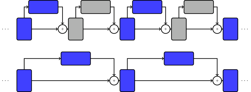
Figure 2: Left: An example of a multilevel hierarchy of ResNets, with the upper level depicted on the top of the figure. Right: An example of decomposing the parameters of DeepONet with branch (brown) and trunk (blue) sub-networks into five subdomains. Each subdomain is depicted in a different color.

5. Aniso: This example considers operator learning using DeepONet [63] in order to approximate a solution of the following parametric anisotropic Poisson’s equation:

$$-\nabla\cdot(K({\eta})\ \nabla z(x)) =f(x),\quad\quad \forall\ x\in\Omega,$$ (77)

$$z =0,\ \forall\ x\in\partial\Omega,$$

where $\Omega:=(-1,1)^{2}$ is the computational domain, with boundary $\partial\Omega$. The symbol $z$ denotes the solution and $f(x):=1$. The diffusion coefficient $K(\eta)$ is the following anisotropic tensor:

$$K(\eta)=\begin{pmatrix}\cos(\alpha)&-\sin(\alpha)\\ \sin(\alpha)&\ \ \ \cos(\alpha)\end{pmatrix}\begin{pmatrix}1&0\\ 0&\beta\end{pmatrix}\begin{pmatrix}\ \ \ \cos(\alpha)&\sin(\alpha)\\ -\sin(\alpha)&\cos(\alpha)\end{pmatrix},$$

parametrized using ${\eta}:=[\alpha,\beta]$. We sample the anisotropic strength ${\beta\in[10^{-6},1]}$ according to ${\log_{10}({\scriptstyle\frac{1}{\beta}})\sim\pazocal{U}[0,6]}$. The angle of the anisotropic direction, denoted by the parameter ${\alpha\in(0,\pi)}$, is sampled as $\alpha\sim\pazocal{U}[0,\pi]$. To construct the dataset, for each value of ${\eta}$, we discretize (77) using a uniform mesh with $34\times 34$ finite elements. The dataset $\pazocal{D}=\{(\eta_{s},\xi_{s},y_{s})\}_{s=1}^{n_{s}}$ is composed of $4{,}250$ training samples and $750$ testing samples. Here, $\xi_{s}\in\mathbb{R}^{n_{c}\times 2}$ denotes the set of coordinates at which the high-fidelity finite element solution $y_{s}\in\mathbb{R}^{n_{c}}$ is evaluated.

The training process is defined as the minimization between the DeepONet output and the target solution, i.e.,

$$\min_{z\in\mathbb{R}^{n}}f(z):=\frac{1}{n_{s}n_{c}}\sum_{s=1}^{n_{s}}\sum_{c=1}^{n_{c}}\big{(}\langle B(\eta_{s};z),T(\xi_{s,c};z)\rangle-y_{s,c}\big{)}^{2},$$ (78)

where $z$ denotes collectively parameters of the DeepONet, consisting of branch (B) and trunk (T) sub-networks. Their outputs $B(\eta_{s};z)\in\mathbb{R}^{Q}$ and $T(\xi_{s,c};z)\in\mathbb{R}^{Q}$ are linearly combined by means of the inner product to approximate the solution of (77) at the location $\xi_{s,c}$ for a given set of parameters $\eta_{s}$. Both sub-networks have dense feedforward architecture with a width of 128, ReLu activation functions, and an output dimension of $Q=126$. The branch consists of 6 layers, while trunk network has 4 layers.

5.2 Implementation and algorithmic setup

For the FEM examples, the benchmark problems and ML-ADAGB2  are implemented using Firedrake [72], while DD-ADAGB2 is implemented using MATLAB. For the DNNs and their training procedures using ML-ADAGB2 and DD-ADAGB2 algorithms, we utilize PyTorch [48].

Our ML-ADAGB2 is implemented in the form of a V-cycle. For ML-ADAGB2, we employ three Taylor iterations on all levels for both pre-and post-smoothing. On the lowest level, i.e., $\ell=0$, we perform five Taylor steps. For DD-ADAGB2, we perform ten decomposition iterations before each Taylor iteration, for all examples except Aniso, where we employ three Taylor iterations and 25 decomposition iterations. For FEM examples, we computed the product $(s_{\ell,k}^{L})^{T}B_{\ell,k}s_{\ell,k}^{L}$ appearing in (9) using gradient finite-differences in complex arithmetic [1], a technique which produces cheap machine-precision-accurate approximations of $(s_{\ell,k}^{L})^{T}H_{\ell,k}s_{\ell,k}^{L}$ without any evaluation of the Hessian $H_{\ell,k}$. For DNNs examples, we consider purely first-order variants of ML-ADAGB2 and DD-ADAGB2, i.e., $B_{\ell,k}=0$ for all $(\ell,k)$. Unless specified otherwise, all evaluations of gradients are exact, i.e., without noise. Parameters $\varsigma$, $\kappa_{\text{1st}}$ and $\kappa_{\text{2nd}}$ are set to $\varsigma=0.01$, $\kappa_{\text{1st}}=0.95$, $\kappa_{\text{2nd}}=10$ for all numerical examples. The learning rate is set to $10^{-2}$ for IndPines (on all levels) and $5\times 10^{-2}$ for Aniso (on all subdomains), as suggested by both single-level and multilevel/domain-decomposition hyperparameters tuning.

The hierarchy of objective functions $\{f_{\ell}\}_{\ell=0}^{r}$ required by the ML-ADAGB2 is constructed for FEM examples by discretizing the original problem using meshes coarsened by a factor of two. Similarly, for the IndPines example, we obtain a multilevel hierarchy by coarsening in time by a factor of two, i.e., each $f_{\ell}$ is then associated with a network of different depths. For all examples, the transfer operators $\{P_{\ell}\}_{\ell=0}^{r-1}$ are constructed using piecewise linear interpolation in space or time; see [29, 56] for details regarding the assembly of transfer operators for ResNets. The restriction operators $\{R_{\ell}\}_{\ell=0}^{r-1}$ are obtained as $R_{\ell}=2^{-d}P_{\ell}^{T}$, where $d$ denotes the dimension of the problem at hand. Moreover, for FEM examples, we enforce the first-order consistency relation (48) on all levels, while no modification to $\{f_{\ell}\}_{\ell=0}^{r}$ is applied for the DNNs examples.

In the case of DD-ADAGB2 algorithm, the function $f_{0}$ is as specified in (59). For FEM examples, each $f^{(p)}$ is created by restricting $f_{r}$ to a subdomain determined by the METIS partitioner [49]. Transfer operators are assembled using the WRAS technique (see Table 1) for the different overlap sizes in our tests. For the Aniso example, the decomposition is obtained by first decomposing the parameters of branch and trunk networks into separate subdomains. The parameters of both sub-networks are further decomposed in a layer-wise manner; see [52, 61] for details regarding the construction of the transfer operators. Figure 2 illustrates multilevel and domain-decomposition hierarchies for our DNNs examples.

For all FEM examples, the initial guess is prescribed as a vector of zeros, which satisfies the boundary conditions and does not violate the bound constraints. For the DNNs examples, the network parameters are initialized randomly using Xavier initialization [31]. Therefore, all reported results for these set of examples are averaged over ten independent runs.

The optimization process for all FEM examples is terminated as soon as $\|\Xi_{r,k}\|<10^{-7}$ or $\|\Xi_{r,k}\|/\|\Xi_{r,0}\|<10^{-9}$. For the IndPines example, the algorithms terminate as soon as $\text{acc}_{\text{train}}>0.98$ or $\text{acc}_{\text{val}}>0.98$. Termination also occurs as soon as $\sum_{i=1}^{15}(\text{acc}_{\text{train}})_{e}-(\text{acc}_{\text{train}})_{e-i}<0.001$ or $\sum_{i=1}^{15}(\text{acc}_{\text{val}})_{e}-(\text{acc}_{\text{val}})_{e-i}<0.001$, where $(\text{acc}_{\text{train/val}})_{e}$ is defined as the ratio between the number of correctly classified samples from the train/validation dataset and the total number of samples in the train/validation dataset for a given epoch $e$. For the Aniso example, the algorithms terminate if the number of epoch exceeds $1,000,000$ or as soon as $\sum_{i=1}^{100}(f_{\text{train}})_{e}-(f_{\text{train}})_{e-i}<0.0001$ or $\sum_{i=1}^{100}(f_{\text{val}})_{e}-(f_{\text{val}})_{e-i}<0.0001$, where $f$ denotes the loss function, as defined in (78).

5.3 Numerical performance of ML-ADAGB2 

We first investigate the numerical performance of multilevel ML-ADAGB2 compared with its single level variant ADAGB2. To assess the performance of the proposed methods fairly, we report not only the number of V-cycles, but also the dominant computational cost associated with gradient evaluations. Let $\pazocal{C}_{r}$ be a computational cost associated with an evaluation of the gradient on the uppermost level, the total computational cost $\pazocal{C}_{\text{ML}}$ for ML-ADAGB2  is evaluated as follows:

$$\pazocal{C}_{\text{ML}}=\sum_{\ell=0}^{r}\frac{n_{\ell}}{n_{r}}\sharp_{\ell}\,\pazocal{C}_{r},$$ (79)

where $\sharp_{\ell}$ describes a number of evaluations performed on a level $\ell$, while the scaling factor $\frac{n_{\ell}}{n_{r}}$ accounts for the difference between the cost associated with level $\ell$ and the uppermost level $r$. Note that for the FEM examples, this estimate accounts for the cost associated with the gradient evaluation required by the finite-difference method used to compute the product $(s_{\ell,k}^{L})^{T}B_{\ell,k}s_{\ell,k}^{L}$. Moreover, we point out that in the case of DNN applications, additional scaling must be applied to account for the proportion of dataset samples used during evaluation.

We begin our numerical investigation by comparing the cost $\pazocal{C}_{\text{ML}}$ of ML-ADAGB2 with ADAGB2. Table 2 presents the numerical results obtained for four benchmark problems, where increasing the number of refinement levels also corresponds to use more levels by ML-ADAGB2. As our results indicate, the cost of ML-ADAGB2 is significantly lower than that of ADAGB2 for all benchmark problems. Notably, the observed speedup achieved by ML-ADAGB2 increases with the number of levels, highlighting the practical benefits of the proposed algorithm for large-scale problems. Moreover, for the IndPines examples, ML-ADAGB2 produces DNN models with accuracy that is comparable to, or even exceeds, that of ADAGB2. Based on our experience, this improved accuracy can be attributed to the fact that the use of hierarchical problem decompositions tends to have a regularization effect [35].

Example	Method		Refinement/ML-ADAGB2  levels
			2	3	4	5
Membrane	ADAGB2		2,704	9,968	36,054	58,880
	ML-ADAGB2		560	588	944	2,102
MinSurf	ADAGB2		2,564	10,400	41,136	103,458
	ML-ADAGB2		684	1,142	2,448	5,224
NeoHook	ADAGB2		67,704	229,512	632,718	$>750,000$
	ML-ADAGB2		3,272	4,272	6,748	14,270
IndPines	ADAGB2	$\text{acc}_{\text{val}}$	90.2%	90.6%	91.2%	91.4%
		$\pazocal{C}_{\text{ML}}$	2,559	2,892	3,718	3,967
	ML-ADAGB2	$\text{acc}_{\text{val}}$	90.1%	91.7%	91.8%	91.9%
		$\pazocal{C}_{\text{ML}}$	1,662	1,220	984	863

Table 2: The total computational cost $\pazocal{C}_{\text{ML}}$ of ML-ADAGB2  and ADAGB2 with respect to increasing number of levels. For IndPines, we also report the highest achieved $\text{acc}_{\text{val}}$.

5.3.1 ML-ADAGB2 with and without active-set approach

As mentioned earlier, the conditions imposed on $R_{\ell}$ and $P_{\ell}$ are extremely general. This flexibility allows us to propose yet another variant of the ML-ADAGB2 algorithm. Motivated by the results reported in [57] and [54] for linear multigrid and multilevel trust-region methods, respectively, we now consider a variant of ML-ADAGB2 that incorporates an active set strategy.

In particular, before ML-ADAGB2 descends to a lower level and performs a recursive iteration (Step 3), we identify the active set using the current iterate $x_{\ell,k}$, i.e.,

$$\pazocal{A}_{\ell,k}(x_{\ell,k}):=\{j\in\{1,\ldots,n_{\ell}\}\ |\ l_{\ell,k,j}=x_{\ell,k,j}\ \ \text{or}\ \ u_{\ell,k,j}=x_{\ell,k,j}\}.$$ (80)

The components of the active set $\pazocal{A}_{\ell,k}$ are then held fixed and cannot be altered by the lower levels. To this end, we define the truncated prolongation operator $\widetilde{P}_{\ell-1}$ as

$$(\widetilde{P}_{\ell-1})_{pt}=\begin{cases}0,\quad&\text{if }\,p\in\pazocal{A}_{\ell,k}(x_{\ell,k}),\\ ({P}_{\ell-1})_{pt},\quad&\text{otherwise}.\end{cases}$$ (81)

Thus, the operator $\widetilde{P}_{\ell-1}$ is obtained from the prolongation operator ${P}_{\ell-1}$ by simply setting the $p$-th row of ${P}_{\ell-1}$ to zero for all $p\in\pazocal{A}_{\ell,k}$. As before, we set $\widetilde{R}_{\ell-1}=2^{-d}\widetilde{P}^{T}_{\ell-1}$. Note that $(\widetilde{P}_{\ell-1}s_{\ell-1})_{p}=0$ for all $p\in\pazocal{A}_{\ell,k}$ and some coarse-level correction $s_{\ell-1,k}=x_{\ell-1,k}-x_{\ell,0}$.

These iteration-dependent truncated transfer operators $\widetilde{P}_{\ell-1}$ and $\widetilde{R}_{\ell-1}$ are then used in place of $P_{\ell-1}$ and $R_{\ell-1}$ during the execution of the recursive iteration (Step 3) of the ML-ADAGB2 algorithm. In addition, we use them to define the coarse-level model $h_{\ell-1}$, by simply restricting the quadratic model from level $\ell$ to level $\ell-1$, as follows:

$$h_{\ell-1}(x_{\ell-1})=(\widetilde{R}_{\ell-1}g_{\ell,k})^{T}s_{\ell-1}+\frac{1}{2}s_{\ell-1}^{T}(\widetilde{R}_{\ell-1}B_{\ell,k}\widetilde{P}_{\ell-1})s_{\ell-1}.$$ (82)

The model $h_{\ell-1}$ is used in place of $f_{\ell-1}$ on the coarse level. This construction ensures that the components of $g_{\ell,k}$ and $B_{\ell,k}$ associated with the active set $\pazocal{A}_{\ell,k}$ are excluded from the definition $h_{\ell-1}$.

Finally, we also point out that, since $\widetilde{P}_{\ell-1}$ has fewer nonzero columns than $P_{\ell-1}$, the resulting lower-level bounds obtained via (12) are less restrictive than those derived using $P_{\ell-1}$. This, in turn, allows for larger steps on the coarse level and leads to improved convergence. To demonstrate this phenomenon, we depict the convergence of the ML-ADAGB2 algorithm with and without the active set strategy for the MinSurf and Membrane examples. Figure 3 illustrates the obtained results. As we can see, the variant with the active set strategy converges significantly faster - approximately by a factor of two. We also observe that convergence is particularly accelerated once the active set on the finest level $\pazocal{A}_{r}$ is correctly identified by the ML-ADAGB2 algorithm.

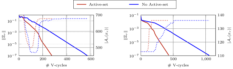
Figure 3: The comparison of the convergence of the ML-ADAGB2 with and without the active-set strategy. Both variants use the Galerkin-based coarse-level models (82). Left: MinSurf (three levels). Right: Membrane (five levels).

5.3.2 Sensitivity of ML-ADAGB2 to the choice of the step-size

This subsection aims to highlight the importance of carefully selecting the step size $\gamma_{\ell,k}$ across all levels and iterations. To this end, we consider the Membrane and MinSurf problems and evaluate the performance of the three-level ML-ADAGB2 algorithm using either an iteration-dependent $\gamma_{\ell,k}$, computed as in (9), or constant $\gamma_{\ell,k}$, choosen from the set $\{0.2,0.5,1.0\}$. As shown in Figure 4 (left), using the iteration-dependent $\gamma_{\ell,k}$ leads to the fastest convergence in terms of the number of required V-cycles. Notably, if fixed $\gamma_{\ell,k}$ is chosen too large, the algorithm may fail to converge due to violation of the sufficient decrease condition, specified in (10).

Figure 4 (right) shows the values of $\gamma_{\ell,k}$ on different levels, as determined by (9). As we can see, the values of $\gamma_{\ell,k}$ vary significantly throughout the iteration process and, typically, larger $\gamma_{\ell,k}$ are determined on lower levels. We also note that when accounting for the cost of gradient evaluation, it is possible to identify a constant $\gamma_{\ell,k}$ for which the overall computational cost $\pazocal{C}_{\text{ML}}$ is comparable to that achieved using iteration-dependent step sizes. This is due to the fact that evaluating $(s_{\ell,k}^{L})^{T}B_{\ell,k}s_{\ell,k}^{L}$ via complex-step finite differences requires an additional gradient evaluation on each iteration. We emphasize, however, that this comparable $\pazocal{C}_{\text{ML}}$ comes at the expense of costly hyper-parameter tuning required to determine an effective $\gamma_{\ell,k}$. Therefore, we restrict the use of fixed step sizes only to the DDN examples, as is common practice in machine learning.

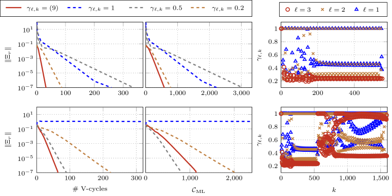
Figure 4: Convergence behavior of ML-ADAGB2 for Membrane (Top) and MinSurf (Bottom) examples with three levels. Left and Middle: Convergence as a function of V-cycles and computational cost for different choices of $\gamma_{\ell,k}$. The values of $\gamma_{\ell,k}$, which remain constant across all levels and iterations, are represented by dashed lines. Right: The values of $\gamma_{\ell,k}$ obtained by means of (9) on different levels during the iteration process. Here, the symbol $k$ denotes the global iteration counter, incremented across all levels and iteration steps.

5.3.3 Sensitivity of ML-ADAGB2  to noise

The main motivation for developing and using OFFO algorithm lies in their performance in the presence of noise. To illustrate the impact of noise on the convergence behaviour of ML-ADAGB2, we first consider the MinSurf problem. Figure 5 (top left) displays the convergence of the algorithm in the absence of noise (red line) and under constant additive noise (blue line). Thus, $g_{\ell,k}=\nabla f(x_{\ell,k})+\epsilon_{\ell,k}$, where each component of random noise vector $\epsilon_{\ell,k}$ is obtained from $\pazocal{N}(0,\sigma_{\ell,k}^{2})$, with $\sigma_{\ell,k}^{2}$ denoting the noise variance. Here, we set  $\sigma_{\ell,k}^{2}=10^{-7}$, for all $(\ell,k)$. As observed, the presence of noise does not significantly affect the convergence until $\|\Xi_{r}\|$ becomes comparable to the noise level. This is particularly beneficial for applications that do not require highly accurate solutions, such as the training of DNNs. However, if a high-accuracy solution is required, it can be obtained by progressively reducing the noise in the gradient evaluations. Following standard practice, one may employ a noise reduction scheduler. For example, we can employ exponential decay scheme [12], with $\sigma_{\ell,k}^{2}=\sigma_{\ell,0}^{2}e^{-\lambda k}$, where we set $\sigma_{\ell,0}^{2}=10^{-7}$ and $\lambda=5\cdot 10^{-2}$. As illustrated by the brown line in Figure 5 (top left), incrementally reducing the noise enables ML-ADAGB2  to converge to a critical point with user prescribed tolerance. Note that the choice of noise reduction scheduler can have a significant impact on the convergence speed.

Understanding ML-ADAGB2’s sensitivity to noise is particularly relevant in the case of DNNs, where inexact gradients, obtained by subsampling, are often used to reduce the iteration cost. Figure 5 (middle and right) demonstrates the convergence of ML-ADAGB2 for the IndPines example, when different numbers of samples are used to evaluate the gradient. In particular, we set the batch size (bs) to 8,100, 1,024, and 128, where 8,100 corresponds to the full dataset. As we can see from the obtained results, ML-ADAGB2 with the full dataset converges the fastest in terms of V-cycles. However, since the cost of evaluating the gradient scales linearly with the number of samples in the batch, ML-ADAGB2  with bs $=128$ is the most cost-efficient. Looking at $\text{acc}_{\text{val}}$ and $\|\Xi_{r}\|$, we observe that ML-ADAGB2 with bs=$8,100$ produces the most accurate DNN. As before, the noise introduced by subsampling can be mitigated during the training process. To this end, we use a learning-rate step decay scheduler [32], in which the learning rate is reduced by a factor of ten at $\pazocal{C}_{\text{ML}}$ equal to $35$ and $55$. As shown in Figure 5 (bottom left), this strategy enhances the quality of the resulting model while maintaining the low computational cost per iteration associated with small-batch gradient evaluations. Moreover, in the long run, the final model accuracy surpasses that achieved by using the whole dataset, highlighting the role of noisy gradients in the early stages of training for improved generalization.

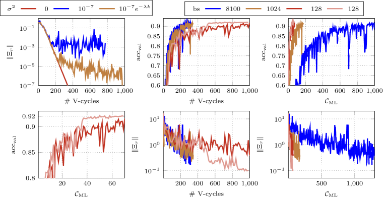
Figure 5: Top Left: Convergence of the ML-ADAGB2 without noise (red), with constant noise (blue, $\sigma^{2}=10^{-7}$) and the noise reduced using the exponential scheduler (brown) for MinSurf (two levels). Bottom Left: Convergence of the ML-ADAGB2 with noise due to gradients subsampled with batch size (bs) of $128$ for IndPines example (three levels). The red color represents results with constant noise, while pink color denotes results with learning rate (lr) scheduler, where lr is dropped by factor of $10$ at $\pazocal{C}_{\text{ML}}$ equal to $35$ and $55$. Middle/Right: Convergence of the ML-ADAGB2 with noise due to gradients subsampled for IndPines example. The blue color stands for exact gradient evaluations, i.e., with the whole dataset (bs=8,100), while brown (bs=1,024) and red/pink (bs=128) consider inexact gradient evaluations.

5.4 Numerical performance of DD-ADAGB2 

In this section, we evaluate the numerical performance of DD-ADAGB2. To this aim, we estimate its total parallel computational cost as

$$\pazocal{C}_{\text{DD}}=\bigg{(}\sharp_{r}\pazocal{C}_{r}\bigg{)}+\bigg{(}\frac{n^{(p)}}{n_{r}}\sharp^{(p)}\pazocal{C}_{0}\bigg{)},$$ (83)

where $n^{(p)}$ denotes the number of degrees of freedom in the largest subdomain, and $\sharp^{(p)}$ represents the number of steps performed on all subdomains. Thus, the first term in (83) accounts for the cost of the Taylor iteration, while the second term corresponds to the cost of subdomain iterations, which can be carried out in parallel.

Table 3 reports the results obtained for the Membrane and MinSurf examples with respect to increasing number of subdomains and overlap. As we can observe, the parallel computational cost $\pazocal{C}_{\text{DD}}$ decreases with increased number of subdomains, reflecting the benefits of possible parallelization. Furthermore, increasing the overlap size contributes to an additional reduction in the computational cost. It is worth noting that the observed parallel speedup of DD-ADAGB2 compared to ADAGB2  is below the ideal. For example, for eight subdomains and an overlap size of two, the speedup is approximately of a factor of four. We attribute this suboptimal theoretical scaling primarily to the cost associated with serial Taylor iterations. As we will discuss in Section 5.5, this limitation can be addressed by developing hybrid multilevel-domain-decomposition algorithms, which effectively combine ML-ADAGB2 and DD-ADAGB2.

Next, we assess the performance of DD-ADAGB2 for training DeepONet. Figure 6 illustrates the results obtained for the Aniso example. Consistent with the previous observations, DD-ADAGB2 achieves a significant speedup compared to standard ADAGB2. Moreover, as for FEM examples, increasing the number of subdomains enables greater parallelism, thereby reducing the parallel computational cost $\pazocal{C}_{\text{DD}}$. Notably, the use of DD-ADAGB2 also yields more accurate DNNs, as evidenced by lower relative errors in the resulting DeepONet predictions. This improvement in accuracy is particularly important, as the reliability of the DeepONet plays a crucial role in a wide range of practical applications.

$\#$ Subdomains/Overlap	Membrane			MinSurf
	0	2	4	0	2	4
1 (ADAGB2)	36,054	–	–	41,136	–	–
2	21,104	20,340	20,230	22,958	21,906	21,868
4	12,864	12,198	12,204	14,162	13,538	12,952
8	9,286	8,574	8,490	9,424	9,132	9,030

Table 3: The parallel computational cost $\pazocal{C}_{\text{DD}}$ of DD-ADAGB2 and ADAGB2  for Membrane (four refinement levels) and MinSurf (four refinement levels) examples.

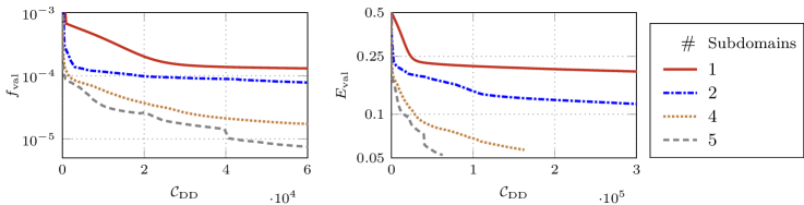
Figure 6: The parallel computational cost $\pazocal{C}_{\text{DD}}$ of ADAGB2($\#$ subdomains=1) and DD-ADAGB2 for Aniso with varying number of subdomains (no overlap). Left: The validation loss $f_{\text{val}}$. Right: The relative validation error ${E_{\text{val}}=1/n_{s}\sum_{s=1}^{n_{s}}(y_{s}^{D}-y_{s})/\|y_{s}\|}$, where $y_{s}^{D}$ is the DeepONet-inferred solution and $y_{s}$ is the target solution. The gradient evaluations are performed using batch-size $bs=1,062$.

5.5 Numerical performance of ML-DD-ADAGB2 

As discussed in Section 5.4, the main benefit of the DD-ADAGB2 algorithm is that it enables the parallelization. However, the cost associated with the sequential Taylor step prohibits the ideal speedup in practice. To improve parallelization capabilities, we draw inspiration from established practices in the domain-decomposition literature [24], where coarse spaces are known to enhance the scalability and robustness of the algorithms at low computational cost. To this end, we now numerically evaluate the effectiveness of a hybrid algorithm, named ML-DD-ADAGB2, which effectively combines the ML-ADAGB2 and DD-ADAGB2 methods. In particular, we replace the Taylor iteration (Step 2) in Algorithm 4 with a call to the ML-ADAGB2 method, i.e., Algorithm 2. Here, ML-ADAGB2 is configured with two levels, where the coarse level is constructed by discretizing the original problem on a mesh coarsened by a factor of eight. This coarse-level approximation is then adjusted using the tau-correction approach, as defined in (48). Our implementation then alternates between performing ten coarse-level iterations and ten decomposition steps. Note, if (6) is satisfied, the recursive steps are replaced with a Taylor iteration on $f_{r}$.

The parallel computational cost of our hybrid ML-DD-ADAGB2 method is given as

$$\pazocal{C}_{\text{ML-DD}}=\sum_{\ell=1}^{r}\frac{n_{\ell}}{n_{r}}\sharp_{\ell}\,\pazocal{C}_{r}+\bigg{(}\frac{n^{(p)}}{n_{r}}\sharp^{(p)}\pazocal{C}_{0}\bigg{)}.$$ (84)

Here, we set $r=2$, i.e., $f_{r}=f_{2}=f$, $f_{1}$ is associated with the coarse-level discretization, and $f_{0}$ is the extended model associated with the subdomains computations, given by (59).

Table 4 reports the results obtained for the Membrane and MinSurf examples. Firstly, we observe that even DD-ADAGB2 algorithm exhibits algorithmic scalability, i.e., the number of V-cycles remains constant with an increasing number of subdomains. This behavior can be observed due to our specific implementation, which alternates ten subdomain steps with one global Taylor iteration. However, as we can see, replacing a Taylor iteration with ten coarse-level iterations leads to a significant improvement in terms of convergence, as indicated by the reduced number of V-cycles. Moreover, the parallel computational cost of ML-DD-ADAGB2 is substantially lower than that of DD-ADAGB2, demonstrating strong potential for our envisioned future work, focusing on integrating ML-DD-ADAGB2 into parallel finite-element and/or deep-learning frameworks.

$\#$ Subd.	Membrane				MinSurf
	DD-ADAGB2		ML-DD-ADAGB2		DD-ADAGB2		ML-DD-ADAGB2
	$\pazocal{C}_{\text{DD}}$	V-cycles	$\pazocal{C}_{\text{ML-DD}}$	V-cycles	$\pazocal{C}_{\text{DD}}$	V-cycles	$\pazocal{C}_{\text{ML-DD}}$	V-cycles
1 (ADAGB2)	36,054	36,054	36,054	36,054	41,136	41,136	41,136	41,136
2	20,340	1,784	586	57	21,906	1,826	3,864	370
4	12,198	1,900	312	58	13,538	1,934	2,024	385
8	8,574	2,158	168	60	9,132	2,032	1,142	406
16	6,318	1,952	92	60	7,806	2,403	612	405

Table 4: The parallel computational cost and the number of V-cycles of DD-ADAGB2, and ML-DD-ADAGB2  with overlap equal to two for Membrane (four refinement levels) and MinSurf (four refinement levels).

6 Conclusions and perspectives

We have proposed an OFFO algorithmic framework inspired by AdaGrad which, unlike the original formulation, can handle bound constraints on the problem variables and incorporate curvature information when available. Furthermore, the framework is designed to efficiently exploit the structural properties of the problem, including hierarchical multilevel decompositions and standard additive Schwarz domain decomposition strategies. The convergence of this algorithm has then been studied in the stochastic setting allowing for noisy and possibly biased gradients, and its evaluation complexity for computing an $\epsilon$-approximate first-order critical point was proved to be ${\pazocal{O}}(\epsilon^{-2})$ (without any logarithmic term) with high probability.

Extensive numerical experiments have been discussed, showing the significant computational gains obtainable when problem structure is used, both in the hierarchical and domain decomposition cases, but also by combining the two approaches. These gains are demonstrated on problems arising from discretized PDEs and machine learning applications such as the training of ResNets and DeepONets. The use of cheap but accurate gradient-based finite-difference approximations for curvature information was also shown to be crucial for numerical efficiency on the PDE-based problems.

While already of intrinsic interest, these results are also viewed by the authors as a step towards efficient, structure exploiting methods for problems involving more general constraints. Other theoretical and practical research perspectives include, for instance, the use of momentum, active constraints’ identification, adaptive noise reduction scheduling and the streamlining of strategies mixing domain decomposition and hierarchical approaches, in particular in the domain of deep neural networks.

References

- [1] R. Abreu, Z. Su, J. Kamm, and J. Gao. On the accuracy of the complex-step-finite-difference method. Journal of Computational and Applied Mathematics, 340:390–403, 2018.
- [2] L. Badea and R. Krause. One-and two-level Schwarz methods for variational inequalities of the second kind and their application to frictional contact. Numerische Mathematik, 120:573–599, 2012.
- [3] L. Badea, X.-C. Tai, and J. Wang. Convergence rate analysis of a multiplicative Schwarz method for variational inequalities. SIAM Journal on Numerical Analysis, pages 1052–1073, 2004.
- [4] L. Badea and J. Wang. An additive Schwarz method for variational inequalities. Mathematics of Computation, 69(232):1341–1354, 2000.
- [5] M. F. Baumgardner, L. L. Biehl, and D. A. Landgrebe. 220 Band AVIRIS Hyperspectral Image Data Set: June 12, 1992 Indian Pine Test Site 3. Purdue University Research Repository, 10(7):991, 2015.
- [6] S. Bellavia, G. Gratton, B. Morini, and Ph. L. Toint. Fast stochastic Adagrad for nonconvex bound-constrained optimization. arXiv:2405.06374, 2025.
- [7] S. Bellavia, G. Gurioli, B. Morini, and Ph. L. Toint. Trust-region algorithms: probabilistic complexity and intrinsic noise with applications to subsampling techniques. EURO Journal on Computational Optimization, 20(100043), 2022.
- [8] S. Bellavia, G. Gurioli, B. Morini, and Ph. L. Toint. The impact of noise on evaluation complexity: The deterministic trust-region case. Journal of Optimization Theory and Applications, 196(2):700–729, 2023.
- [9] S. Bellavia, N. Krejić, and N. Krklec Jerinkić. Subsampled inexact Newton methods for minimizing large sums of convex functions. arXiv:1811.05730, 2018.
- [10] A. Berahas, L. Cao, and K. Scheinberg. Global convergence rate analysis of a generic line search algorithm with noise. SIAM Journal on Optimization, 31:1489–1518, 2021.
- [11] J. Blanchet, C. Cartis, M. Menickelly, and K. Scheinberg. Convergence rate analysis of a stochastic trust region method via supermartingales. INFORMS Journal on Optimization, 1(2):92–119, 2019.
- [12] G. Bottou, F. Curtis, and J. Nocedal. Optimization methods for large-scale machine learning. SIAM Review, 60(2):223–311, 2018.
- [13] A. Brandt and C. W. Cryer. Multigrid algorithms for the solution of linear complementarity problems arising from free boundary problems. SIAM Journal on Scientific and Statistical Computing, 4(4):655–684, 1983.
- [14] W. L. Briggs, V. E. Henson, and S. F. McCormick. A Multigrid Tutorial. SIAM, Philadelphia, USA, 2nd edition, 2000.
- [15] X. C. Cai and D. E. Keyes. Nonlinearly preconditioned inexact Newton algorithms. SIAM Journal on Scientific Computing, 24(1):183–200, 2002.
- [16] X.-C. Cai and M. Sarkis. A restricted additive Schwarz preconditioner for general sparse linear systems. SIAM Journal on Scientific Computing, 21(2):792–797, 1999.
- [17] H. Calandra, S. Gratton, E. Riccietti, and X. Vasseur. On high-order multilevel optimization strategies. SIAM Journal on Optimization, 31(1):307–330, 2021.
- [18] R. G. Carter. On the global convergence of trust region methods using inexact gradient information. SIAM Jounal on Numerical Analysis, 28(1):251–265, 1991.
- [19] C. Cartis and K. Scheinberg. Global convergence rate analysis of unconstrained optimization methods based on probabilistic models. Mathematical Programming A, 159(2):337–375, 2018.
- [20] B. Chang, L. Meng, E. Haber, F. Tung, and D. Begert. Multi-level residual networks from dynamical systems view. arXiv:1710.10348, 2017.
- [21] F. Chaouqui, M. J. Gander, P. M. Kumbhar, and T. Vanzan. Linear and nonlinear substructured restricted additive Schwarz iterations and preconditioning. Numerical Algorithms, 91(1):81–107, 2022.
- [22] G. Ciaramella, F. Nobile, and T. Vanzan. A multigrid solver for PDE-constrained optimization with uncertain inputs. Journal of Scientific Computing, 101(1):13, 2024.
- [23] V. Dolean, M. J. Gander, W. Kheriji, F. Kwok, and R. Masson. Nonlinear preconditioning: How to use a nonlinear Schwarz method to precondition Newton’s method. SIAM Journal on Scientific Computing, 38(6):A3357–A3380, 2016.
- [24] V. Dolean, P. Jolivet, and F. Nataf. An introduction to domain decomposition methods: algorithms, theory, and parallel implementation. SIAM, 2015.
- [25] M. Domorádová and Z. Dostál. Projector preconditioning for partially bound-constrained quadratic optimization. Numerical Linear Algebra with Applications, 14(10):791–806, 2007.
- [26] J. Duchi, E. Hazan, and Y. Singer. Adaptive subgradient methods for online learning and stochastic optimization. Journal of Machine Learning Research, 12, July 2011.
- [27] M. C. Ferris and O. L. Mangasarian. Parallel variable distribution. SIAM Journal on Optimization, 4(4):815–832, 1994.
- [28] A. Frommer and D. B. Szyld. An algebraic convergence theory for restricted additive Schwarz methods using weighted max norms. SIAM Journal on Numerical Analysis, 39:463–479, 2002.
- [29] L. Gaedke-Merzhäuser, A. Kopaničáková, and R. Krause. Multilevel minimization for deep residual networks. In Proceedings of French-German-Swiss Optimization Conference (FGS’2019), 2021.
- [30] E. Gelman and J. Mandel. On multilevel iterative methods for optimization problems. Mathematical Programming, 48(1-3):1–17, 1990.
- [31] X. Glorot and Y. Bengio. Understanding the difficulty of training deep feedforward neural networks. Journal of Machine Learning Research, 9:249–256, 2010.
- [32] I. Goodfellow, Y. Bengio, and A. Courville. Deep Learning. MIT Press, 2016.
- [33] S. Gratton, S. Jerad, and Ph. L. Toint. Complexity of Adagrad and other first-order methods for nonconvex optimization problems with bounds constraints. arXiv:2406.15793, 2024.
- [34] S. Gratton, S. Jerad, and Ph. L. Toint. Parametric complexity analysis for a class of first-order Adagrad-like algorithms. Optimization Methods and Software, (to appear), 2025.
- [35] S. Gratton, A. Kopaničáková, and Ph. L. Toint. Multilevel objective-function-free optimization with an application to neural networks training. SIAM Journal on Optimization, 33(4):2772–2800, 2023.
- [36] S. Gratton, V. Mercier, E. Riccietti, and Ph. L. Toint. A block-coordinate approach of multi-level optimization with an application to physics-informed neural networks. Computational Optimization and Applications, (to appear), 2025.
- [37] S. Gratton, M. Mouffe, Ph. L. Toint, and M. Weber-Mendonça. A recursive trust-region method in infinity norm for bound-constrained nonlinear optimization. IMA Jounal of Numerical Analysis, 28(4):827–861, 2008.
- [38] S. Gratton, A. Sartenaer, and Ph. L. Toint. Recursive trust-region methods for multiscale nonlinear optimization. SIAM Journal on Optimization, 19(1):414–444, 2008.
- [39] S. Gratton and Ph. L. Toint. A note on solving nonlinear optimization problems in variable precision. Computational Optimization and Applications, 76(3):917–933, 2020.
- [40] S. Gratton, L.N. Vicente, and Z. Zhang. Optimization by space transformation and decomposition. Technical report, Polytechnic University of Hong Kong, Hong Kong, 2019.
- [41] Ch. Groß. A unifying theory for nonlinear additively and multiplicatively preconditioned globalization strategies: convergence results and examples from the field of nonlinear elastostatics and elastodynamics. PhD thesis, Bonn University, Bonn, Germany, 2009.
- [42] Ch. Groß and R. Krause. A new class of non-linear additively preconditioned trust-region strategies: Convergence results and applications to non-linear mechanics. Technical Report 904, Institute for Numerical Simulation, University of Bonn, INS preprint, 2009.
- [43] Ch. Groß and R. Krause. On the globalization of ASPIN employing trust-region control strategies - convergence analysis and numerical examples. Technical Report 2011-03, Universita della Svizzera Italiana, Lugano, CH, 2011. Also available as arXiv:2104.05672v1.
- [44] E. Haber and L. Ruthotto. Stable architectures for deep neural networks. Inverse Problems, 34(1):014004, 2017.
- [45] W. Hackbusch and H. D. Mittelmann. On multi-grid methods for variational inequalities. Numerische Mathematik, 42(1):65–76, 1983.
- [46] M. Holst. Algebraic Schwarz theory. Technical report, Department of Applied Mathematics and CRPC, California Institute of Technology, California, USA, 1994.
- [47] R. H. W. Hoppe and R. Kornhuber. Adaptive multilevel methods for obstacle problems. SIAM journal on numerical analysis, 31(2):301–323, 1994.
- [48] S. Imambi, K. B. Prakash, and G. R. Kanagachidambaresan. Pytorch. Programming with TensorFlow: solution for edge computing applications, pages 87–104, 2021.
- [49] G. Karypis and V. Kumar. Metis: A software package for partitioning unstructured graphs, partitioning meshes, and computing fill-reducing orderings of sparse matrices. Retrieved from the University Digital Conservancy, https://hdl.handle.net/11299/215346, 1997.
- [50] D. Kingma and J. Ba. Adam: A method for stochastic optimization. In Proceedings in the International Conference on Learning Representations (ICLR), 2015.
- [51] M. Kočvara and S. Mohammed. A first-order multigrid method for bound-constrained convex optimization. Optimization Methods and Software, 31(3):622–644, 2016.
- [52] A. Kopaničáková, H. Kothari, G. E. Karniadakis, and R. Krause. Enhancing training of physics-informed neural networks using domain decomposition–based preconditioning strategies. SIAM Journal on Scientific Computing, 46(5):S46–S67, 2024.
- [53] A. Kopaničáková and R. Krause. A recursive multilevel trust region method with application to fully monolithic phase-field models of brittle fracture. Computer Methods in Applied Mechanics and Engineering, 360:112720, 2020.
- [54] A. Kopaničáková and R. Krause. A Multilevel Active-Set Trust-Region (MASTR) Method for Bound Constrained Minimization. In Domain Decomposition Methods in Science and Engineering XXVI, pages 355–363. Springer, 2023.
- [55] A. Kopaničáková. On the use of hybrid coarse-level models in multilevel minimization methods. In International Conference on Domain Decomposition Methods, pages 303–310. Springer, 2022.
- [56] A. Kopaničáková and R. Krause. Globally convergent multilevel training of deep residual networks. SIAM Journal on Scientific Computing, 45(0):S254–S280, 2022.
- [57] R. Kornhuber. Monotone multigrid methods for elliptic variational inequalities I. Numerische Mathematik, 69(2):167–184, 1994.
- [58] R. Kornhuber and R. Krause. Adaptive multigrid methods for Signorini’s problem in linear elasticity. Computing and Visualization in Science, 4(1):9–20, 2001.
- [59] H. Kothari, A. Kopaničáková, and R. Krause. Nonlinear Schwarz preconditioning for nonlinear optimization problems with bound constraints. In International Conference on Domain Decomposition Methods, pages 319–326. Springer, 2022.
- [60] R. Krause. A nonsmooth multiscale method for solving frictional two-body contact problems in 2D and 3D with multigrid efficiency. SIAM Journal on Scientific Computing, 31(2):1399–1423, 2009.
- [61] Y. Lee, A. Kopaničáková, and G. E. Karniadakis. Two-level overlapping additive schwarz preconditioner for training scientific machine learning applications. arXiv:2406.10997, 2024.
- [62] B. Leimkuhler, T. Vlaar, T. Pouchon, and A. Storkey. Better training using weight-constrained stochastic dynamics. arXiv:2106.10704, 2021.
- [63] L. Lu, P. Jin, G. Pang, Z. Zhang, and G. Karniadakis. Learning nonlinear operators via deeponet based on the universal approximation theorem of operators. Nature machine intelligence, 3(3):218–229, 2021.
- [64] L. Lu, R. Pestourie, W. Yao, Z. Wang, F. Verdugo, and S. G. Johnson. Physics-informed neural networks with hard constraints for inverse design. SIAM Journal on Scientific Computing, 43(6):B1105–B1132, 2021.
- [65] J. Mandel. A multilevel iterative method for symmetric, positive definite linear complementarity problems. Applied Mathematics and Optimization, 11(1):77–95, 1984.
- [66] O. L. Mangasarian. Parallel gradient distribution in unconstrained optimization. SIAM Journal on Control and Optimization, 33(6):1916–1925, 1995.
- [67] S. G. Nash. A multigrid approach to discretized optimization problems. Optimization Methods and Software, 14:99–116, 2000.
- [68] J. Park. Additive Schwarz methods for convex optimization as gradient methods. SIAM Journal on Numerical Analysis, 58(3):1495–1530, 2020.
- [69] J. Park. Accelerated additive Schwarz methods for convex optimization with adaptive restart. Journal of Scientific Computing, 89(3):58, 2021.
- [70] J. Park. Additive Schwarz methods for convex optimization with backtracking. Computers & Mathematics with Applications, 113:332–344, 2022.
- [71] A. F. Queiruga, N. B. Erichson, D. Taylor, and M. W. Mahoney. Continuous-in-depth neural networks. arXiv:2008.02389, 2020.
- [72] F. Rathgeber, D. A. Ham, L. Mitchell, M. Lange, F. Luporiniand A. T. T. McRae, G.-T. Bercea, G. R. Markall, and P. H. J. Kelly. Firedrake: automating the finite element method by composing abstractions. ACM Transactions on Mathematical Software (TOMS), 43(3):1–27, 2016.
- [73] H. Robbins and S. Monro. A stochastic approximation method. The Annals of Mathematical Statistics, 22(3):400––407, 1951.
- [74] U. Trottenberg, C. W. Oosterlee, and A. Schuller. Multigrid methods. Academic press, 2001.
- [75] K. Trotti, S. A. Cruz, A. Kopaničáková, and R. Krause. Parallel trust-region approaches in neural network training. Mathematical Optimization for Machine Learning: Proceedings of the MATH+ Thematic Einstein Semester 2023, page 107, 2025.
- [76] M. Vallejos. MGOPT with gradient projection method for solving bilinear elliptic optimal control problems. Computing, 87(1-2):21–33, 2010.
- [77] J. Youett, O. Sander, and R. Kornhuber. A globally convergent filter-trust-region method for large deformation contact problems. SIAM Journal on Scientific Computing, 41(1):B114–B138, 2019.