Plane-layer Rayleigh-Bénard convection up to $Ra=10^{11}$: Near-wall fluctuations and role of initial conditions

Abstract

We study temperature and velocity fluctuations in turbulent Rayleigh-Bénard convection through direct numerical simulations in a three-dimensional plane layer of height $H$ with horizontal periodic boundary conditions and aspect ratio $4H\times 4H\times H$. The analysis is performed for Rayleigh numbers $10^{5}\leq Ra\leq 10^{11}$ and Prandtl number $Pr=0.7$. First, the study systematically summarizes the height-dependent statistics of velocity and temperature fluctuations and reports corresponding scalings with the Rayleigh number. Secondly, we include an analysis on the role of coherent and incoherent flow regions near the wall for the global heat transfer. Thirdly, we investigate the dependence of turbulent heat and momentum transfer on additional finite-amplitude shear flow modes in the initial condition at time $t=0$, which either decay unforced with respect to time in a long transient or remain existent when a steady volume forcing in the momentum balance of the Boussinesq model is added. In the latter case, logarithmic near-wall layers for mean velocity and temperature are formed. In all cases, no impact on the global turbulent heat and momentum transfer within the error bars is detected, even though the shear mode amplitude is of the order of the characteristic free-fall velocity.

Keywords: Turbulent convection, Direct Numerical Simulation

1 Introduction

Rayleigh-Bénard convection (RBC) is a benchmark problem of fluid turbulence, that has withstood the test of time to remain a fruitful field of research. Spurred by its relevance to atmospheric flows, industrial cooling and heat exchange systems, planetary boundary layers and a host of other applications, RBC continues to be a subject of both experimental and numerical studies [1, 2, 3, 4]. The canonical form of RBC invokes a plane layer of fluid confined between two parallel, infinitely extended horizontal plates. Unstable stratification requires a colder top and hotter bottom plate [5]. Under the influence of gravity which acts along the vertical direction, a buoyancy-driven convective flow arises, transferring the heat between the plates, on average from the bottom to the top. The driving coherent flow structures for this heat transfer are the thermal plumes, whose structure and impact on flow properties has been a subject of considerable scrutiny [6, 7, 8]. It is understood that these plumes originate from thermal instabilities in the boundary regions near the walls [9, 10] for sufficiently high temperature gradients. Understanding their role for turbulent heat and momentum transfer requires a height-dependent investigation of the fluctuation statistics of both temperature and velocity, which is one focus of the present work. A similar study for confined convection in a closed cylinder was also performed by [11].

Although thermal plumes drive the convective turbulence, the dynamics is not purely plume-dominated. In [12], it was shown that the viscous near-wall region is a patchwork of local shear-dominated coherent and plume-detaching incoherent regions in a practically constant percentage area ratio of 40:60, which is in line with the absence of a global unidirectional mean flow in this plane-layer RBC configuration. The near-wall layers of temperature and, in particular, of velocity are dominated by fluctuations for the whole range of Rayleigh numbers. In [13], it was then shown that thermal plumes are organized in a hierarchical and self-similar network that gets coarser with increasing wall distance. The network dynamics can be described as a continued coagulation and reformation process. A basic building block of the dynamics are local marginally unstable segments of the thermal boundary layer, which has been studied in several models [10, 14, 15]. This self-organization of the near-wall flow in extended plane layers seems to be imperative for the efficient transport of heat that follows closely a classical 1/3 scaling with respect to Rayleigh number; it leads to near-wall layers that are different from standard boundary layers in wall-bounded shear flows.

The dichotomy of coherent (shear dominance or plume impact) and incoherent (plume detachment) regions, particularly their role for the heat transfer, was also investigated for two-dimensional RBC in [16, 17]. Furthermore, confined convection in closed cells at an aspect ratio close of 1 or smaller is dominated by a large-scale circulation (LSC) [2]. A dynamically analogous description of the boundary region flow into plume-detachment and post-plume phases also shows there significant differences between both regimes [18]. In the present work, we will explore the strategy of isolating these two sides of the boundary layer flow by thresholding the wall-shear stress field in order to compare the findings with those of [12]. One of our goals in disentangling the coherent and incoherent regions of the boundary layer is to quantify differences in heat transfer between these two regions. This is a second motivation point for the present study.

It has been hypothesized that the turbulent flow passes through a transition at very high Rayleigh number $Ra$ (which quantifies the thermal driving in RBC), which leads to a heat transfer scaling law $Nu\sim Ra^{\gamma}$ with an exponent larger than the classical one, $\gamma>1/3$. The Nusselt number $Nu$ is a dimensionless measure of turbulent heat transfer. This regime of RBC is termed the “ultimate regime” [19, 20]. Significant efforts have been expended towards attaining very high Rayleigh numbers in turbulent convection in laboratory experiments [1, 21, 22, 23, 24] and three-dimensional numerical simulations [25, 26, 12, 27] to detect this regime. See also [28, 29, 30, 31, 32, 4] for different conclusions on its existence. In [31] and later in [33, 4], it was proposed that such a regime change, if existing, is connected to a transition of the near-wall layers — analogous to a subcritical transition to turbulence in wall-bounded shear flows [34]. This would imply the hysteresis-type coexistence of two global flow regimes in turbulent RBC [33], as the laminar and turbulent state in wall-bounded shear flows with the latter state trapped in a chaotic repeller that is formed by a skeleton of linearly unstable exact coherent states [35, 36]. To carry such a loose analogy even further: a coexistence would be in line with a sensitive dependence on the specific form of finite-amplitude perturbations that trigger transitions between both macrostates; see for example [37, 38] for wall-bounded flows.

A resulting further motivation for the present work is thus to investigate the dependence of the statistically stationary turbulent RBC state on the initial condition. Do different conditions kick the RBC system into different turbulent states with different near-wall dynamics? If yes, how do they affect the global transport? DNS of RBC typically start with a linear temperature profile across the layer, the diffusive equilibrium state. This state is infinitesimally perturbed. Here, we add a shear mode $u_{x}(y,t=0)=\tilde{A}_{i}\sin(\pi y)$ in agreement with incompressibility and boundary conditions at finite amplitude $\tilde{A}_{i}$ to compare the long-term evolution of initially different RBC runs. This idea is then further extended by adding a steady volume forcing $f_{x}$ to the momentum balance that maintains this shear mode $u_{x}(y)$, see e.g. [39]. In all cases, the Nusselt and Reynolds number, the global measures of heat and momentum transfer, remains unchanged within the error bars compared to the standard case with $u_{x}(y,t=0)=0$ and $f_{x}=0$. Interestingly, for the run with $f_{x}\neq 0$, we detect a logarithmic region of the mean temperature and velocity profiles, similar to previous mixed convection studies in pressure-driven plane Poiseuille [40, 41] or plane Couette geometries [42, 43], both with heated and smooth walls. We will show that the logarithmic near-wall layer, which is formed for the case of additional steady volume forcing, does not practically affect the global transport properties within the error bar.

In section 2, we present the numerical model. In section 3, we summarize the height-dependent statistics of temperature and velocity, which complements our earlier study in [12]. Section 4 summarizes the refined analysis with respect to coherent and incoherent regions. Section 5 discusses the impact of different initial conditions and the additional volume forcing. We finally summarize and conclude our findings in section 6.

2 Governing equations and numerical method

We solve the incompressible Navier-Stokes equations with the Boussinesq approximation coupling the velocity and temperature fields, ${\bm{u}}({\bm{x}},t)$ and $T({\bm{x}},t)$ respectively. These partial differential equations are solved in the non-dimensional form,

$$\frac{\partial{\bm{u}}}{\partial t}+({\bm{u}}\cdot{\bm{\nabla}}){\bm{u}}=-{\bm{\nabla}}p+T\hat{{\bm{z}}}+\sqrt{\frac{Pr}{Ra}}\,\nabla^{2}{\bm{u}},$$ (1)

$$\frac{\partial T}{\partial t}+({\bm{u}}\cdot{\bm{\nabla}})T=\frac{1}{\sqrt{PrRa}}\,\nabla^{2}T,$$ (2)

$${\bm{\nabla}}\cdot{\bm{u}}=0.$$ (3)

The two dimensionless parameters are Rayleigh number $Ra$ and Prandtl number $Pr$, which are defined as

$$Ra=\frac{g\alpha\Delta TH^{3}}{\nu\kappa}\quad\mathrm{and}\quad Pr=\frac{\nu}{\kappa}.$$ (4)

Here, $g$ denotes the acceleration due to gravity, $\alpha$ is the thermal expansion coefficient, $\Delta T$ is the temperature difference between the hot and cold plates,$H$ is the vertical separation between the plates, $\nu$ is the kinematic viscosity, and $\kappa$ is the thermal diffusivity. These dimensional quantities are also used to define the free-fall velocity, $U_{f}=\sqrt{\alpha g\Delta TH}$, as the characteristic unit of the velocity field. Correspondingly, characteristic length, time and temperature scales are $H$, $H/U_{f}$, and $\Delta T$ respectively.

The RBC flow reacts with a turbulent heat and momentum transfer to the set of input parameters, $\{Ra,Pr\}$. The corresponding dimensionless numbers are the Nusselt number $Nu$ for the turbulent heat and the Reynolds number $Re$ for the turbulent momentum transfer. They are given by (all quantities are dimensionless)

$$Nu=-\frac{\partial\langle T\rangle_{A,t}}{\partial z}\Bigg{|}_{z=0}\quad\mbox{and}\quad Re=\sqrt{\frac{Ra}{Pr}}U^{v}_{\rm rms}\,,$$ (5)

where $\langle\cdot\rangle_{A,t}$ is a combined average over cross section $A$ and simulation time $t$ in statistically steady state. The root mean square velocity $U^{v}_{\rm rms}=\langle{\bm{u}}^{2}\rangle^{1/2}_{V,t}$ with a combined volume-time average $\langle\cdot\rangle_{V,t}$. The Boussinesq equations are solved in a Cartesian box of size $L\times L\times H$, where $L$ denotes both the length and width of the box. We choose a domain of aspect ratio $\Gamma=L/H=4$ for our simulations, so that the cross-sectional area $A=16$ in dimensionless units. Together with the periodic boundary conditions on the sides, this setup aims to approximate an infinitely extended plane layer of fluid confined between the top and bottom no-slip walls, which are isothermally maintained at $T$ and $T+\Delta T$ respectively. Further details on this choice of parameters are presented in  [12].

The governing equations are solved using spectral element method (SEM), where the computational domain is discretized into finite elements, on each of which the fields are approximated by Lagrangian interpolation basis functions in all three space dimensions, offering an accuracy comparable to spectral methods [44]. We use the GPU-accelerated SEM solver NekRS [45], which is a descendant of the Nek5000 code. Our simulations span a range of $Ra$ from $10^{5}$ to $10^{11}$ at a fixed Prandtl number of $Pr=0.7$. Of particular focus is the case at $Ra=10^{9}$, with which we present additional studies on the effect of initial condition and forced shear flow in section 5 and section 5.2 respectively. The simulations are performed with sufficient spectral resolution, and the planar averaged profiles are also well converged. This is described and discussed in detail in  [12]. There, we also showed that the thermal boundary layers are well-resolved, with at least 16 spectral collocation points within them for all the cases.

3 Height-dependent statistics of velocity and temperature

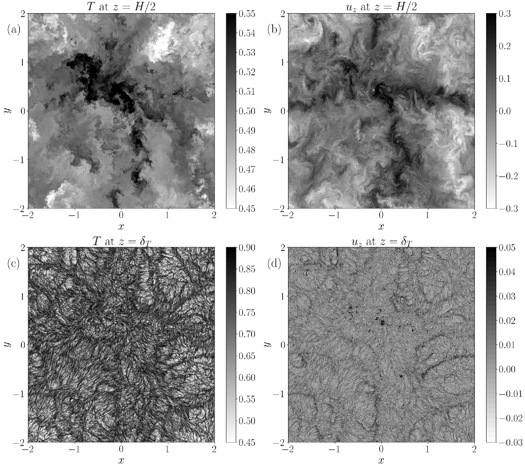
Figure 1: Contours of temperature (a, c) and vertical component of velocity (b, d) on a horizontal cross-section ($xy$-plane) from a snapshot at $Ra=10^{11}$. The upper and lower rows shows the fields at $z=H/2$ and $\delta_{T}$ respectively. The structure of the flow is more sharply delineated at the thermal boundary layer where plumes dominate the flow. Whereas at the midplane in the bulk, the fields are thoroughly turbulent and well-mixed. Appropriate colorbar cut-offs have been chosen for increased contrast and clear visibility of structures.

The structure of convective flow is markedly different in the bulk and the boundary layer, especially at higher Rayleigh numbers where the boundary layers become significantly thinner. As a result, a systematic study of thermal convection requires one to disentangle the two regions and their contributions to the overall heat and momentum transfer [2, 11]. We define the thermal boundary layer thickness $\delta_{T}$ at both walls as the distances of the local maxima of temperature fluctuations from their respective walls, and this value is practically same as $1/(2Nu)$ which we detailed in [12].

Figure 1 demonstrates the distinction between bulk and BL flow using the temperature $T$ and vertical velocity component $u_{z}$ for a snapshot at $Ra=10^{11}$. A well-defined and fine-grained plume structure is visible in the thermal boundary layer at $z=\delta_{T}$ in the lower row, whereas in the bulk at $z=H/2$ (upper row), the temperature field is well-mixed and the velocity field is turbulent. Nevertheless, we also note that there is no sharp transition from bulk to boundary layer. Rather, there is a self-similar hierarchy of plumes which successively aggregate as we transition from boundary layer to bulk, see [13] for this analysis. As a result, it is important to investigate the fluctuation intensities and statistics of velocity and temperature fields at different heights. In the next subsections, we choose heights of the analysis planes that are multiples of the boundary layer thickness, $\delta$, to obtain the scaling of fluctuation intensities with $Ra$ and probability distribution functions. This thickness $\delta$ of the near-wall layer can be determined even in absence of a global mean flow. We will thus use two thickness scales, one based on the temperature, $\delta_{T,{\rm rms}}$, and one based velocity fluctuation profiles, $\delta_{U,{\rm rms}}$.

3.1 Vertical profiles of velocity and temperature fluctuations

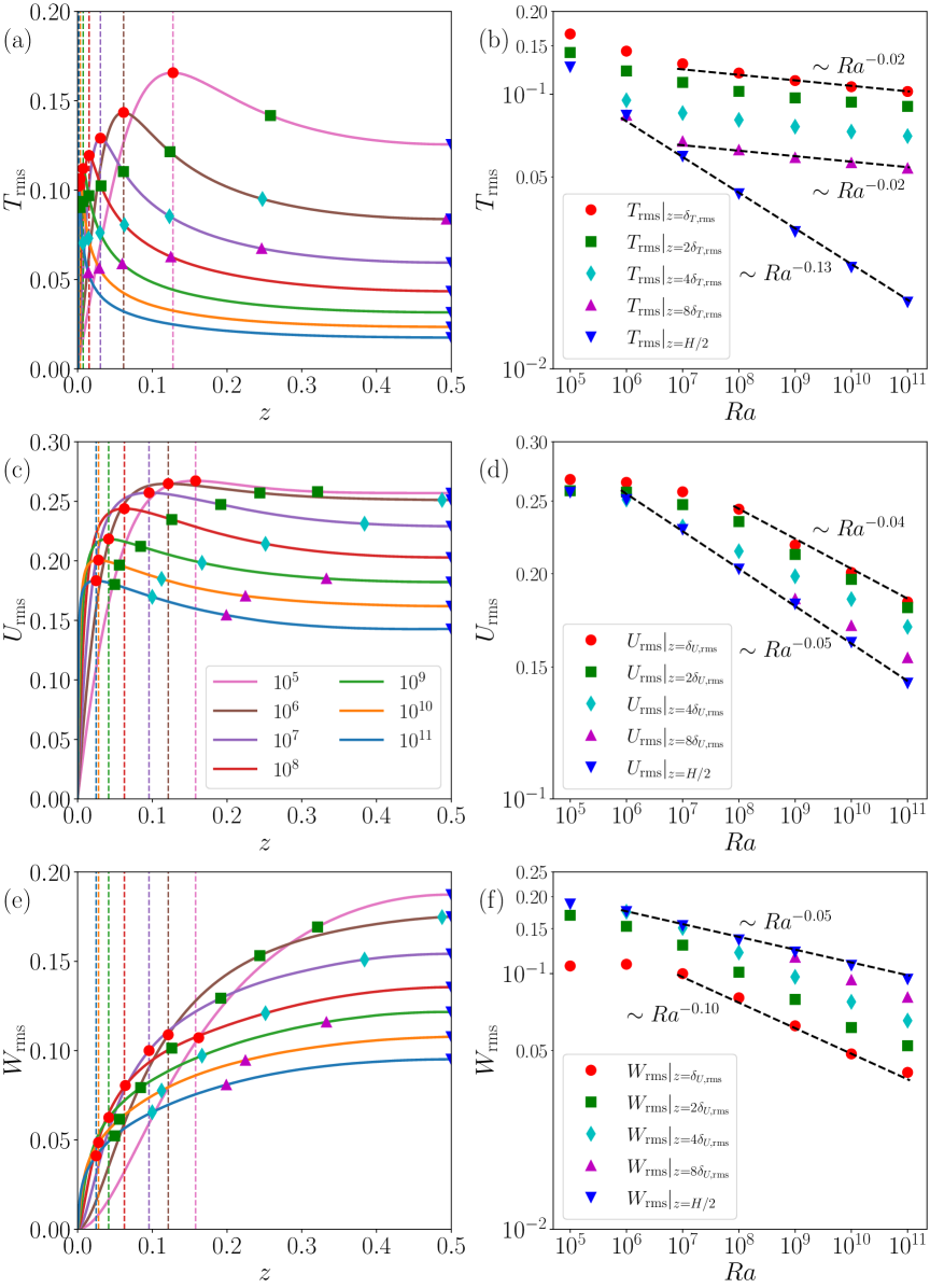
Figure 2: (a) Profiles of temperature fluctuations, $T_{\mathrm{rms}}$, averaged across area $A$ and runtime $t$, for all Rayleigh numbers. The symbols indicate the values of these profiles at $z=\delta_{T,\mathrm{rms}}$ (red circles), $z=2\delta_{T,\mathrm{rms}}$ (green squares), $z=4\delta_{T,\mathrm{rms}}$ (cyan diamonds), $z=8\delta_{T,\mathrm{rms}}$ (purple triangles), and $z=H/2$ (blue inverted triangles).(b) Scaling of the indicated values of $T_{\mathrm{rms}}$ in (a) versus $Ra$. (c) Corresponding profiles of velocity fluctuations, $U_{\mathrm{rms}}$ with symbols marked in the same manner as in (a). The heights are now multiples of the momentum boundary region thickness, $\delta_{U,\mathrm{rms}}$. (d) Scaling of the indicated values of $U_{\mathrm{rms}}$ in (c) versus $Ra$. Similarly, the fluctuation profiles and scaling of the vertical velocity component, $u_{z}$, are shown in panels (e) and (f) respectively.

$Ra$	$\delta_{T,\mathrm{rms}}$	$\delta_{U,\mathrm{rms}}$	$T_{\mathrm{rms}}$, $\delta=\delta_{T,\mathrm{rms}}$
			$\delta$	$2\delta$	$4\delta$	$8\delta$	$H/2$
$10^{5}$	$1.28\times 10^{-1}$	$1.58\times 10^{-1}$	$0.166$	$0.142$	-	-	$0.126$
$10^{6}$	$6.16\times 10^{-2}$	$1.21\times 10^{-1}$	$0.143$	$0.121$	$0.095$	$0.084$	$0.084$
$10^{7}$	$3.06\times 10^{-2}$	$9.57\times 10^{-2}$	$0.129$	$0.110$	$0.085$	$0.067$	$0.059$
$10^{8}$	$1.55\times 10^{-2}$	$6.26\times 10^{-2}$	$0.119$	$0.102$	$0.081$	$0.063$	$0.043$
$10^{9}$	$7.47\times 10^{-3}$	$4.16\times 10^{-2}$	$0.112$	$0.097$	$0.076$	$0.059$	$0.032$
$10^{10}$	$3.62\times 10^{-3}$	$2.80\times 10^{-2}$	$0.106$	$0.094$	$0.073$	$0.056$	$0.023$
$10^{11}$	$1.80\times 10^{-3}$	$2.48\times 10^{-2}$	$0.102$	$0.090$	$0.070$	$0.054$	$0.017$

Table 1: The boundary region heights $\delta_{T,\mathrm{rms}}$ and $\delta_{U,\mathrm{rms}}$ used to plot the scalings of figure 2, along with the values of $T_{\mathrm{rms}}$ at different heights. For the lowest $Ra$, the heights are sufficiently large such that $4\delta_{T,\mathrm{rms}}$ and above lie beyond $z=H/2$.

$Ra$	$U_{\mathrm{rms}}$, $\delta=\delta_{U,\mathrm{rms}}$					$W_{\mathrm{rms}}$, $\delta=\delta_{U,\mathrm{rms}}$
	$\delta$	$2\delta$	$4\delta$	$8\delta$	$H/2$	$\delta$	$2\delta$	$4\delta$	$8\delta$	$H/2$
$10^{5}$	$0.267$	$0.258$	-	-	$0.257$	$0.107$	$0.169$	-	-	$0.187$
$10^{6}$	$0.265$	$0.257$	$0.251$	-	$0.251$	$0.109$	$0.153$	$0.175$	-	$0.175$
$10^{7}$	$0.257$	$0.247$	$0.231$	-	$0.229$	$0.100$	$0.129$	$0.151$	-	$0.154$
$10^{8}$	$0.244$	$0.235$	$0.214$	-	$0.203$	$0.080$	$0.101$	$0.121$	-	$0.136$
$10^{9}$	$0.218$	$0.212$	$0.198$	$0.185$	$0.182$	$0.063$	$0.079$	$0.097$	$0.116$	$0.122$
$10^{10}$	$0.201$	$0.196$	$0.185$	$0.170$	$0.162$	$0.049$	$0.062$	$0.078$	$0.095$	$0.108$
$10^{11}$	$0.183$	$0.180$	$0.170$	$0.154$	$0.143$	$0.041$	$0.052$	$0.066$	$0.081$	$0.095$

Table 2: The values of $U_{\mathrm{rms}}$ and $W_{\mathrm{rms}}$ at different heights for all $Ra$, plotted in figure 2. The heights are multiples of $\delta_{U,\mathrm{rms}}$, which is listed in table 1. Since $\delta_{U,\mathrm{rms}}$ tends to be much larger than $\delta_{T,\mathrm{rms}}$, we see that $8\delta_{U,\mathrm{rms}}>H/2$ even for $Ra$ as high as $10^{8}$.

The planar-averaged profiles of the root mean square (rms) temperature and velocity fluctuations are shown in figure 2. The rms temperature fluctuations are calculated as $T_{\mathrm{rms}}(z)=\sqrt{\langle\theta^{2}({\bm{x}},t)\rangle_{A,t}}$, where $\theta({\bm{x}},t)=T({\bm{x}},t)-\langle T(z)\rangle_{A,t}$. The maxima of the $T_{\mathrm{rms}}$ profiles are located close to the top and bottom plates, and the average distance between the maxima and their respective walls is a measure of the thermal boundary layer thickness, $\delta_{T,\mathrm{rms}}$. These heights are indicated with dashed lines along with the $T_{\mathrm{rms}}$ profiles in figure 2 (a), colored according to their respective $Ra$ values. Similarly, the rms velocity fluctuations are calculated as $U_{\mathrm{rms}}(z)=\sqrt{\langle{\bm{u}}^{2}({\bm{x}},t)\rangle_{A,t}}$, and the $U_{\mathrm{rms}}$ profiles also have their maxima close to the two plates, yielding a corresponding momentum (or viscous) boundary thickness of $\delta_{U,\mathrm{rms}}$, see figure 2 (c). Additionally, fluctuations in the vertical component of velocity are calculated as $W_{\mathrm{rms}}(z)=\sqrt{\langle u_{z}^{2}({\bm{x}},t)\rangle_{A,t}}$, for which the maxima are always at the midplane of the convection cell at $z=H/2$. The $W_{\mathrm{rms}}$ profiles are plotted in figure 2 (e) along with $\delta_{U,\mathrm{rms}}$ lines, similar to panel (c) of the same figure.

For a height-dependent analysis of the fluctuation profiles, we track the rms values at 5 heights, $z=\delta_{F,\mathrm{rms}}$, $2\delta_{F,\mathrm{rms}}$, $4\delta_{F,\mathrm{rms}}$, $8\delta_{F,\mathrm{rms}}$, and $H/2$, where $F=\{T,U\}$ for the temperature and velocity profiles. These five locations are marked by filled symbols – red circles, green squares, cyan diamonds, purple triangles, and blue inverted triangles, respectively, in figure 2. The values of fluctuation profiles corresponding to these heights are tabulated in tables 1 and 2 for temperature and velocity, respectively. Table 1 also lists the values of $\delta_{T,\mathrm{rms}}$ and $\delta_{U,\mathrm{rms}}$. The blank values in these tables correspond to those heights, which exceed the half height of $H/2$.

The scaling of the rms values at the chosen heights for all $Ra$ are plotted in figure 2 in panels (b), (d) and (f) for temperature, total velocity and vertical velocity, respectively. At sufficiently high Rayleigh numbers of $Ra\geq 10^{8}$, all data follow a $Ra$-scaling law at all chosen heights and for all quantities. For the midplane, the scaling range is even extended to lower Rayleigh numbers. All near-wall data follow similar scalings for $T_{\rm rms}$ and $U_{\rm rms}$ with practically no $Ra$-dependence. In case of $W_{\rm rms}$, the small scaling exponent increases from -0.10 at the edge of the boundary layer to -0.05 at the midplane. This scaling, together with the decreased amplitude towards the bulk, seems to be connected with the ongoing detachment of the thermal plumes and their subsequent rise into the bulk. The total velocity fluctuations (which include the horizontal velocity components) at the midplane display practically the same scaling as those above the boundary layer, again with a systematically decreased magnitude towards the bulk. Only the temperature fluctuations at the midplane have a smaller scaling exponent with -0.13 and thus a stronger $Ra$-dependence. See also [12] for a comparison with other previous investigations.

Figure 3: Probability density functions (PDF) of the temperature fluctuations $\theta$ (top row), velocity magnitude $U=|{\bm{u}}|$ (middle row) and vertical velocity component $u_{z}$ (bottom row), sampled at horizontal cross-sectional $x$-$y$ planes at increasing heights of $z=\delta_{T},~2\delta_{T},~4\delta_{T},\mathrm{and}~8\delta_{T}$ (left to right) for all $Ra$ values. The $y$ axis is logarithmic in the upper row; it is linear in the middle and bottom rows.

3.2 Probability density function of velocity and temperature fluctuations

The probability density functions (PDFs) of velocity and temperature fluctuations show marked variations with Rayleigh number – the distributions tend to become narrower with increasing $Ra$, as seen in figure 3. In the figure, the PDFs of the temperature fluctuation $\theta$ are shown for cross-sectional planes taken at 4 different heights from the bottom plate, namely $z=\delta_{T,\mathrm{rms}}$, $2\delta_{T,\mathrm{rms}}$, $4\delta_{T,\mathrm{rms}}$, and $8\delta_{T,\mathrm{rms}}$, in the upper row. The corresponding PDF of the velocity magnitude $U=|{\bm{u}}|$ and vertical velocity component $u_{z}$ are presented in the middle and bottom rows respectively. Note that unlike in the previous section, where the velocity fluctuations were sampled at multiples of $\delta_{U,\mathrm{rms}}$, the PDFs are calculated at planes corresponding to $\delta_{T,\mathrm{rms}}$ here. The PDFs for temperature are distinctly different at the edge of the thermal boundary layer, as compared with the other heights. The range of bins of the distributions is kept constant for all the heights to clearly indicate their narrowing or widening, as we transition from the wall to the bulk.

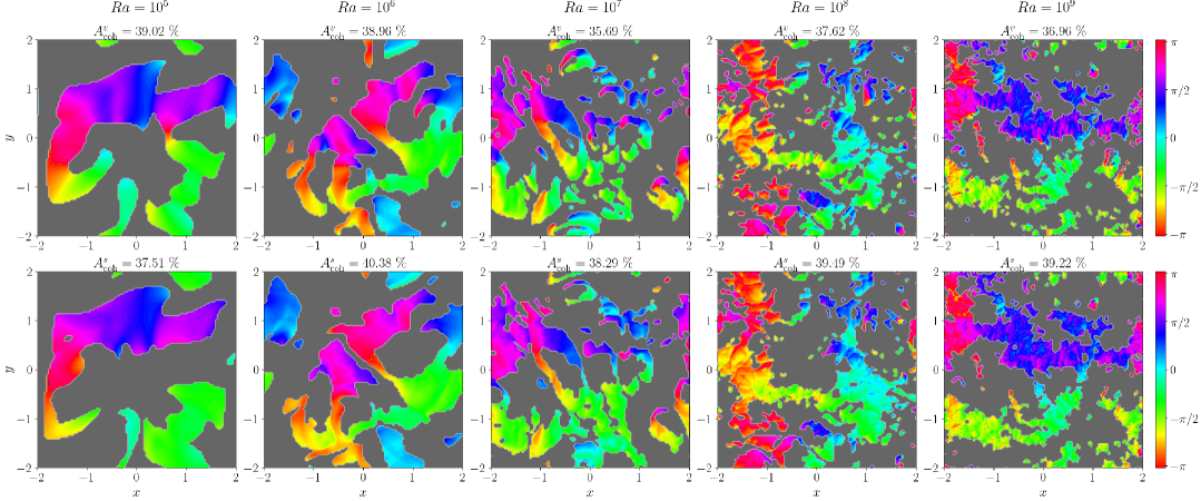
Figure 4: Decomposition of the boundary region flow field into shear-dominated coherent sections and plume-dominated incoherent sections at the thermal boundary layer height $z=\delta_{T}$. Two methods are compared for $Ra$ ranging from $10^{5}$ to $10^{9}$ - thresholding the rms horizontal velocity, $U_{h}$ (top row), and the horizontal shear-stress, $S_{h}$ (bottom row). The corresponding area fractions of the coherent regions are also indicated as $A^{v}_{\mathrm{coh}}$ and $A^{s}_{\mathrm{coh}}$ respectively.

4 Nusselt number in coherent and incoherent boundary layer regions

The flow in the boundary region of a plane-layer unconfined RBC is understood to be a patchwork of shear-dominated (coherent) and plume-dominated (incoherent) regions. The in-plane horizontal velocity, $\mathbf{u_{h}}=(u_{x},u_{y})$, was shown to be a reliable measure for identifying such coherent and incoherent areas in [12]. This is done by breaking up the 2D flow-field in the $x$-$y$ plane at the edge of the thermal boundary layer, $z=\delta_{T}$, into $100\times 100$ disjoint tiles of area $A_{i}=A/10^{4}$. The area-averaged planar rms velocities are computed for individual tiles, as well as across the whole plane, by

$$U^{i}_{h}=\sqrt{\langle u_{x}^{2}+u_{y}^{2}\rangle_{A_{i}}}\quad\mathrm{and}\quad U_{h}=\sqrt{\langle u_{x}^{2}+u_{y}^{2}\rangle_{A}}.$$ (6)

The tiles with $U^{i}_{h}\geq U_{h}$ indicate shear-dominated regions, whereas the tiles with $U^{i}_{h}<U_{h}$ are labeled as plume-dominated. Alternatively, one can also take the shear stress field at the no-slip plates to isolate shear dominated sections from the rest. We investigate this alternative criterion by focusing on the horizontal shear-stress field, $\mathbf{s_{h}}=(s_{x},s_{y})$, where

$$s_{x}=\left|\frac{\partial u_{x}}{\partial z}\right|\quad\mathrm{and}\quad s_{y}=\left|\frac{\partial u_{y}}{\partial z}\right|.$$ (7)

Similar to the velocity-based criterion, the local and global area-averaged rms shear stress, namely $S^{i}_{h}$ and $S_{h}$ respectively, are calculated over disjoint tiles.

Figure 4 compares these two methods of decomposing the horizontal velocity field at the edge of the thermal boundary layer, $z=\delta_{T}$, for four Rayleigh numbers ranging from $10^{5}\leq Ra\leq 10^{9}$. Both methods give a consistent and similar distribution of coherent and incoherent regions. The area fraction of the region with coherent flow is the ratio between the summed area of shear-dominated tiles and the total cross-sectional area, $A$. The area fractions calculated from $\mathbf{u_{h}}$ and $\mathbf{s_{h}}$ are denoted $A^{v}_{\mathrm{coh}}$ and $A^{s}_{\mathrm{coh}}$ respectively. The instantaneous values of the area fractions are indicated for the snapshots in figure 4, and these are consistent with the average coherent area fraction of 40 % observed earlier in [12]. This underlines the robustness of this decomposition approach.

We also investigate the effect of shear flow on local heat transfer by computing the corresponding temperature gradients at the wall. Consequently, we define the two locally area-averaged Nusselt numbers for these two regions as

$$Nu_{\mathrm{coh}}=-\left\langle\frac{\partial T}{\partial z}\bigg{|}_{z=0}\right\rangle_{A\in A^{v}_{\mathrm{coh}},t}\qquad Nu_{\mathrm{incoh}}=-\left\langle\frac{\partial T}{\partial z}\bigg{|}_{z=0}\right\rangle_{A\in A^{v}_{\mathrm{incoh}},t}.$$ (8)

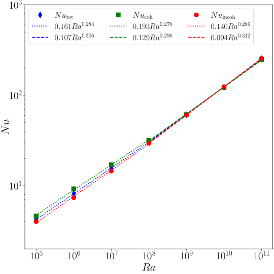
Figure 5: Scaling of $Nu$ in the coherent and incoherent regions of the boundary region for $10^{5}\leq Ra\leq 10^{11}$. The contribution to global heat transport from the shear-dominated regions decreases with increasing $Ra$. In the high-Rayleigh-number regime for $Ra>10^{8}$, scaling of $Nu(Ra)$ is closest to $1/3$ in the plume dominated regions, whereas the shear-dominated regions display a smaller scaling exponent.

$Ra$	$Nu_{\mathrm{tot}}$	$Nu_{\mathrm{coh}}$	$Nu_{\mathrm{incoh}}$
$10^{5}$	$4.26\pm 0.18$	$4.63\pm 0.24$	$4.02\pm 0.21$
$10^{6}$	$8.14\pm 0.18$	$9.25\pm 0.32$	$7.38\pm 0.21$
$10^{7}$	$15.58\pm 0.26$	$17.07\pm 0.48$	$14.56\pm 0.22$
$10^{8}$	$30.47\pm 0.44$	$31.83\pm 0.82$	$29.54\pm 0.38$
$10^{9}$	$60.73\pm 0.65$	$61.04\pm 0.97$	$60.54\pm 0.80$
$10^{10}$	$122.96\pm 1.24$	$121.60\pm 1.55$	$123.92\pm 1.41$
$10^{11}$	$253.04\pm 1.52$	$249.50\pm 2.29$	$255.53\pm 2.16$

Table 3: The values of Nusselt number $Nu$ in the plume-dominated ($Nu_{\mathrm{incoh}}$) and shear-dominated regions ($Nu_{\mathrm{coh}}$) compared with the one taken over the whole horizontal cross section area ($Nu_{\mathrm{tot}}$). The data are plotted in figure 5.

The scaling of $Nu_{\mathrm{coh}}$ and $Nu_{\mathrm{incoh}}$ are shown in figure 5 along with their corresponding fits, both for the moderate ($Ra\leq 10^{8}$) and higher ($Ra\geq 10^{8}$) Rayleigh numbers. These values are also summarized in table 3. Interestingly, the shear-dominated sections have a higher heat-transfer at low to moderate $Ra$ values up to $Ra=10^{9}$. This trend reverses at $Ra\geq 10^{10}$, where the plume-dominated regions contribute to a greater share of the overall heat transport. We note that similar decompositions were performed in the case of two-dimensional RBC by Zhu et al. [16] and He et al. [17] for periodic side boundaries and solid side walls, respectively. Plume-dominated regions were further broken down into plume ejection and plume impact regions and differences in the local turbulent heat transfer and the mean profiles of velocity and temperature were identified.

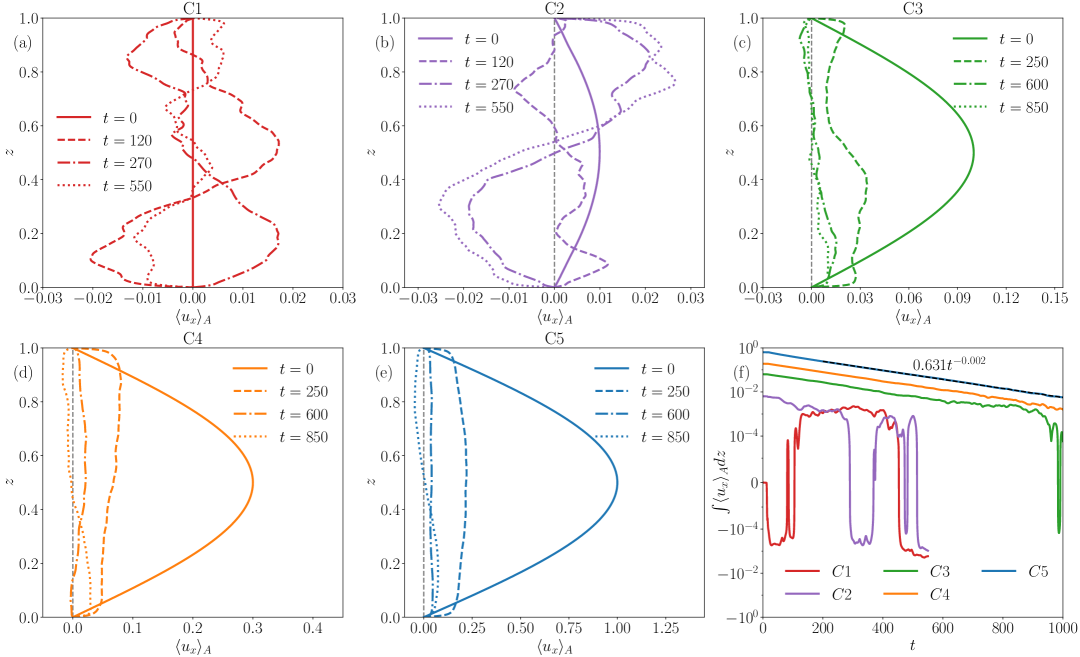
Figure 6: Snapshots of the planar-averaged mean vertical profiles of the $x$-component of velocity at 4 instances of non-dimensional time, and the rates of their decay. Cases C1 through C5 are shown in panels (a) to (e) respectively. The last panel shows the temporal variation of the area under the velocity profile integrated along the vertical $z$-direction. The area is positive when there is a net mean flow in $x$-direction and vice-versa. See also table 4 for the parameters of the runs.

5 Long-term evolution for different initial conditions

5.1 Initial condition with global sinusoidal shear flow mode

We now delve deeper into the effect of plume- and shear-dominated regions on the overall turbulent heat transfer in RBC by considering the case, where a finite-amplitude unidirectional shear flow is initially imposed along an arbitrarily chosen direction, which is w.l.o.g. the $x$ direction in the following. Over a sufficiently long duration, this initial flow will decay and the buoyancy-driven convective flow will dominate. We retain the $\Gamma=4$ domain with periodic horizontal extents, and impose a sinusoidal flow along the positive $x$-axis with a profile of $u_{x}(z)=\tilde{A}_{i}\sin(\pi z)$. This flow is added to the standard initial condition, the infinitesimally perturbed linear temperature profile. The chosen Rayleigh number for this study is $Ra=10^{9}$; the Prandtl number is unchanged at $Pr=0.7$.

To clearly quantify the effect of the additional initial flow mode, we consider 5 cases with different values of initial flow amplitude $\tilde{A}_{i}$, named C1, C2, C3, C4 and C5, with $\tilde{A}_{i}=0$, 0.01, 0.1, 0.3 and 1.0 respectively. Of these, C1 represents the standard RBC case. All 5 cases have a linear temperature profile $T(z)=1-z$ as the initial condition for the temperature. The initial velocity profiles of the cases listed above can be observed by the solid lines in panels (a) to (e), respectively, of figure 6.

Figure 6 (f) traces the temporal variation of the mean flow along $x$-direction, which is calculated as $\int_{0}^{1}\langle u_{x}\rangle_{A}dz$. This is a flow rate. For the cases with weak or no initial shear flow, C1 and C2, we observe a randomly fluctuating mean flow indicating that the convective current dominates across the domain. Nevertheless, in case C2 it takes a short duration for the initial shear flow mode to decay. The buoyancy-driven flow takes over only after approximately 200 free-fall time units. The cases C3, C4 and C5 have a sufficiently stronger initial flow amplitude, such that it requires more than 550 free-fall time units for a full decay. Consequently, these cases were run for longer total integration times to quantify the time it takes for the signature of initial shear flow to disappear completely. The temporal decay of the shear flow mode follows a consistent power law of $t^{-0.002}$, with prefactors that increase with the amplitude $\tilde{A}_{i}$ of the initial sinusoidal profile. We observe that C3 begins to deviate from this power law after approximately 650 free-fall times. After nearly 950 units, the mean flow begins to fluctuate around zero mean, like in cases C1 and C2. Furthermore, cases C4 and C5 require far longer times than 1000 units for the flow to recover a completely buoyancy-dominated dynamics. In all cases, the shear mode, which was initially exited, is not sustained by the nonlinear couplings of the degrees of freedom of the turbulent flow.

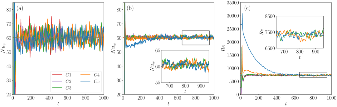
Figure 7: Time-series of the (a) volume-averaged Nusselt number, $Nu_{v}$, (b) area-averaged wall Nusselt number, $Nu_{w}$, and (c) Reynolds number, $Re$, for the 5 cases with varying amplitudes of initial sinusoidal forcing at $Ra=10^{9}$. The large fluctuations in $Nu_{v}$ mask the lower heat transfer in the strongly shear-dominated case, which is made visible by the $Nu_{w}$ plot. As the effect of the strong shear flow subsides, the Nusselt number increases to the expected value of 60.5 for $Ra=10^{9}$ [12].

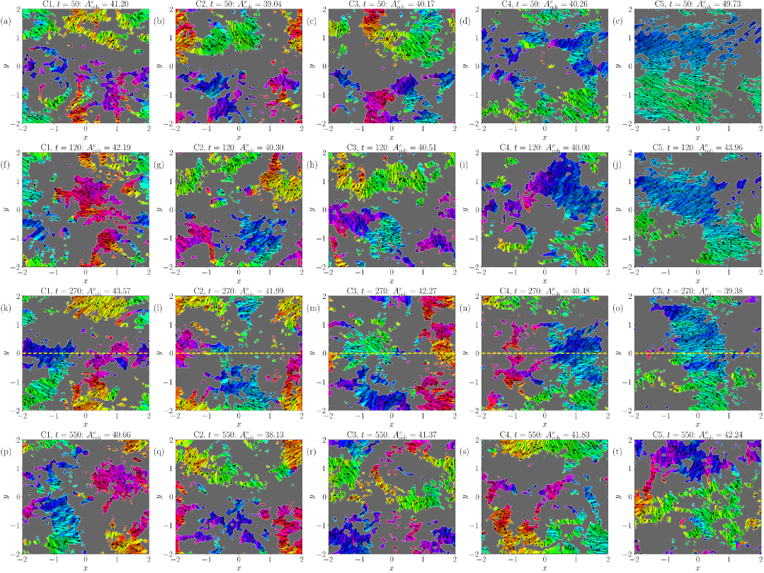
Figure 8: Decomposition of flow field at the thermal boundary layer, $z=\delta_{T}$, into shear and plume-dominated sections with the same color mapping as in figure 4. The five columns from left to right show cases C1, C2, C3, C4 and C5 respectively. The four rows from top to bottom are snapshots of each case at $t=50$, 120, 270 and 550 respectively. Interestingly, there are significant plume dominated sections even in the cases with strong shear flow. This is explained by the overall $U_{\mathrm{rms}}$ threshold for splitting the flow being elevated when there is a background flow. The dashed yellow line in the third row indicates the vertical planes shown in figure 9.

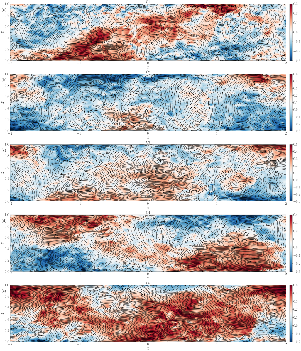
Figure 9: Structure of flow field on the vertical $xz$-plane at $y=0$ for cases C1 through C5 at $t=270$. Although there is a strong initial shear flow in C5, the mean flow adopts a wavy-structure, alternatively grazing the top and bottom plates, allowing for pockets of reverse flow, driven by the thermal plumes. This explains the patches of reverse flow observed on the plate in figure 8 and the relatively low area fraction of shear-dominated patches.

The globally averaged dimensionless quantities Reynolds number, $Re$, and Nusselt number, $Nu$, represent the total momentum and heat flux, respectively. They were defined in (5). The intensity of turbulence increases with $Ra$ and consequently so does the $Re$. We now consider two approaches for calculating the Nusselt number – from the wall temperature gradient and from the convective transport of temperature – which are represented as $Nu_{w}$ and $Nu_{v}$ respectively,

$$Nu_{w}=-\frac{\partial\langle T\rangle_{A,t}}{\partial z}\bigg{|}_{z=0}\quad\mbox{and}\quad Nu_{v}=1+\sqrt{RaPr}\langle u_{z}T\rangle_{V,t}.$$ (9)

Nusselt number $Nu_{w}$ corresponds to $Nu$ in (5). The notation has been changed to distinguish this number from $Nu_{v}$. The temporal variation of these dimensionless quantities is plotted in figure 7. The volume-averaged heat flux typically tends to fluctuate greatly as observed in figure 7 (a). This masks the differences in heat transfer across the five cases. Nevertheless, $Nu_{w}$ in (b), which varies to lesser degree, highlights the differences between the shear-dominated and plume-dominated states of the flow. In the case of case C5, for the first 200 free-fall times when the system has a significant mean flow, the Nusselt number is noticeably lower. The Reynolds number $Re$ in panel (c) indicates higher values for stronger mean flows as expected, and all cases converge to the common value of approximately 7350 within the error bars.

Now, we apply again the decomposition of the flow in the near-wall region into coherent and incoherent regions, as already presented in section 4, to the shear-flow cases at times $t=$ 50, 120, 270 and 550, all of which lie within the range of durations common to all five cases. Figure 8 shows this decomposition for cases C1 to C5 arranged column-wise from left to right, and at increasing units of time from top to bottom. The underlying contours show the flow angle, similar to figure 4, and the streamlines illustrate the velocity field. For C5 at $t=50$, the area fraction of the coherent flow region is 50% and not 40% as in all other cases. One would nominally expect a higher area fraction for such a strong initial mean flow at such an early stage of the evolution of flow. All cases still seem to have a significant plume-dominated region despite the imposed shear flow. One reason for this is the elevated threshold value of $U_{\mathrm{rms}}$ due to background flow.

Figure 9 provides a more compelling explanation for the smaller area fraction even with applied shear. The figure shows the vertical cross-section ($x$-$y$ plane) of the flow at half of the spanwise extension, $y=0$, for cases C1 through C5 arranged from top to bottom. All snapshots are taken at time $t=270$. We see that the flow gets organized in a wavy structure that grazes the top and bottom plates in an alternating way as it moves from left to right. This reorganization of RBC flow under imposed shear has also been observed in the case with Couette-flow shearing [42, 43]. As a result, the flow near the walls has alternating regions of shear flow with pockets of buoyancy-driven recirculating flow in between, bringing down the area fraction of coherent flow.

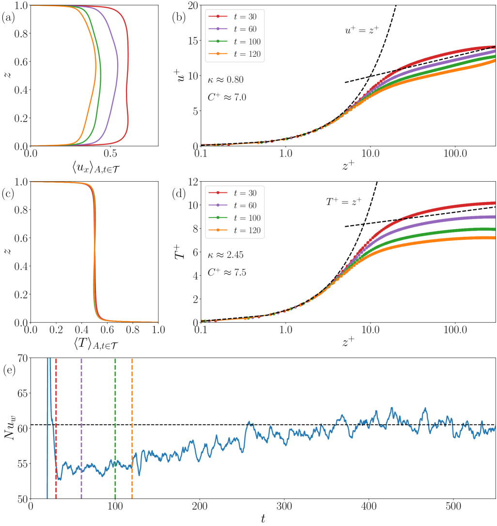
Figure 10: (a) Planar-averaged profiles of $x$-component of velocity, $\langle u_{x}\rangle_{A,t\in\mathcal{T}}$, for case C5, at four time instants, $t=$ 30, 60, 100 and 120. Here, $\mathcal{T}$ is a short time-averaging window of 10 free-fall times centered around the respective $t$ values. (b) The corresponding rescaled velocity profiles in wall units along with the viscous-sublayer and log-law regimes indicated with dashed black lines. (c) Planar-averaged profiles of temperature, $\langle T\rangle_{A,t\in\mathcal{T}}$, again for case C5, at the same instants as in panels (a) and (b). (d) The corresponding rescaled temperature profiles in wall units. (e) The four instants highlighted in the previous panels are indicated with dashed vertical lines in the time-series of $Nu_{w}$ to demonstrate the impact on the global heat transport.

From the planar-averaged profiles of the streamwise velocity component in figure 6 we observe that as the high-amplitude initial flow decays for case C5 in panel (e), the profile at $t=250$ appears to have a thin near-wall mean profile similar to that observed in wall-bounded shear flows. We therefore focus on the initial decay of C5 in figure 10, where we investigate potential signatures of logarithmic mean velocity profile. Four snapshots are chosen at $t=$ 30, 60, 100 and 120; the data for which are plotted in red, purple, green and orange respectively. To smooth out rapid fluctuations in the profiles, a short averaging window of 10 free-fall times, $\mathcal{T}$, is used to compute time averages. From the velocity profiles $\langle u_{x}\rangle_{A,t\in\mathcal{T}}$ shown in (a), we observe the D-shaped profile at $t=30$.

Similar to the analysis of free-stream boundary layers [46], we compute the friction velocity, $u_{\tau}$, and the inner length scale, $l^{+}$, as

$$u_{\tau}=\sqrt{\frac{\tau_{w}}{\rho}},\quad\quad l^{+}=\frac{\nu}{u_{\tau}},\quad\quad\mbox{where}\quad\quad\tau_{w}=\mu\frac{d\langle u_{x}\rangle_{A,t\in\mathcal{T}}}{dz}.$$ (10)

Here $\mu$ and $\rho$ are the dynamic viscosity and mass density, respectively, so that $\nu=\mu/\rho$. Using $u_{\tau}$ and $l^{+}$, the velocity and length scales are rescaled to obtain the profiles in terms of wall units, $u^{+}=\langle u_{x}\rangle_{A,t\in\mathcal{T}}/u_{\tau}$, and $z^{+}=z/l^{+}$. The resulting profiles are plotted in figure 10 (b) along with the viscous sub-layer curve, which is given by $u^{+}=z^{+}$. The logarithmic law of the wall follows to

$$u^{+}(z^{*})=\frac{1}{\kappa_{w}}\log{z^{+}}+C\,.$$ (11)

The von Kármán constant $\kappa_{w}$ and the offset $C$ are expected to be approximately 0.4 and 5.5, respectively, for standard wall-bounded turbulent shear flows, such as pipe flow, plane Poiseuille flow, or plane Couette flow [46]. Although the viscous-sublayer is well-resolved — each dot on the curves represents a collocation point — and since the flow is steadily decaying, a logarithmic profile is detected for a very time interval and a very small range only. Afterwards, the profiles deviate. As a result, we obtain $\kappa_{w}$ and $C$ as 0.75 and 6.5 respectively, as annotated in the figure.

Furthermore, we rescale the temperature profiles shown in panel (c) using $u_{\tau}$ given in (10) along with the wall temperature unit, $T_{\tau}$, defined in terms of the wall heat flux as

$$T_{\tau}=\frac{Q}{u_{\tau}},\quad\quad\mbox{where}\quad\quad Q=\frac{Nu_{w}\kappa\Delta}{H},\quad\quad\mbox{and}\quad\quad l^{+}=\frac{\kappa}{u_{\tau}}.$$ (12)

The resulting rescaled profiles are also plotted in figure 10 (d), with the diffusive sublayer and the logarithmic region marked by dashed black lines as in panel (b). A well-developed logarithmic scaling is not observable. The situation is thus similar to the velocity case.

Finally, the time series of the wall-based Nusselt number, $Nu_{w}$, is reproduced in the last panel (e) with dashed vertical lines colored in correspondence with the four time instants, at which the profiles have been obtained. We observe that the heat flux is reduced when the velocity profiles indicate a turbulent shear-driven boundary layer. Since the heat flux is driven mainly by plumes, the strong shear disrupts this vertical transport of heat, resulting in a lower Nusselt number value. To further investigate the effect of shear flow on heat transport, we consider the case of steady horizontal velocity forcing in the next subsection, which is applied to maintain the shear flow mode.

5.2 Evolution with steadily forced sinusoidal shear flow mode

Figure 11: Comparison of the decay of mean flow for the sinusoidally forced case along with cases C4 and C5 shown previously in figure 6 (f). The forced case attains steady mean flow at $t\approx 750$, and the mean shear flow rate at steady state is approximately 0.037 (marked with dashed black line). The decay of the flow is also shown in linear scale (b) to highlight the difference in mean flow rate between the forced and decaying cases.

We now impose a continuous shear force along the positive $x$-direction, ${\bm{f}}=f(z){\bm{e}}_{x}$, to maintain a shear flow across the hot and cold plates. This additional term is introduced in the dimensional form of the momentum conservation equation, (1), presented earlier in section 2,

$$\frac{\partial{\bm{u}}}{\partial t}+({\bm{u}}\cdot{\bm{\nabla}}){\bm{u}}=-\frac{{\bm{\nabla}}p}{\rho}+\alpha g(T-T_{\rm ref})\hat{{\bm{z}}}+\nu\nabla^{2}{\bm{u}}+{\bm{f}}.$$ (13)

The imposed body force is conservative, so that ${\bm{f}}=-\nu\nabla^{2}{\bm{U}}_{0}$ [47, 39]. The total velocity field can therefore be decomposed into a mean flow with fluctuations, ${\bm{u}}={\bm{U}}_{0}+{\bm{u}}^{\prime}$, where

$${\bm{U}}_{0}(z)=A_{f}\sin{\left(\frac{\pi z}{H}\right)}\hat{{\bm{x}}},\qquad\qquad{\bm{f}}=-\nu\nabla^{2}{\bm{U}}_{0}=\frac{\nu\pi^{2}}{H^{2}}{\bm{U}}_{0}.$$ (14)

We note that this steady shear has exactly the same form as the mode, which was added to the initial condition in cases C2 to C5 in the last subsection. In dimensionless form, we obtain the following form of the momentum equation,

$$\frac{\partial{\bm{u}}}{\partial t}+({\bm{u}}\cdot{\bm{\nabla}}){\bm{u}}=-{\bm{\nabla}}p+T\hat{{\bm{z}}}+\sqrt{\frac{Pr}{Ra}}\,\nabla^{2}{\bm{u}}+A_{f}\pi^{2}\sqrt{\frac{Pr}{Ra}}\sin{(\pi z)}\hat{{\bm{x}}}.$$ (15)

We use the same flow setup as in the previous sections, with a Cartesian box of $\Gamma=4$, at $Ra=10^{9}$ and $Pr=0.7$. The amplitude $A_{f}=1.0$ used in the forcing term is chosen such that it corresponds to the initial flow amplitude of C5. To accelerate the relaxation to the statistically stationary mixed convection state, the initial amplitude in C6 is actually chosen to $\tilde{A}_{6}=0.3$ corresponding to C4.

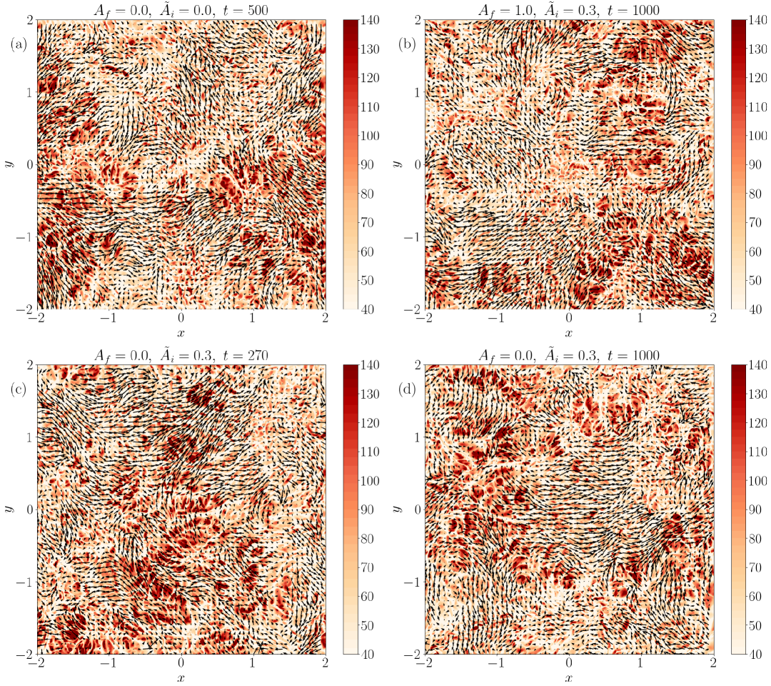
Figure 12: Instantaneous velocity fields of cases C1, C4 and C6 at $z=2\delta_{T}$ at selected times. The vector arrows project ${\bm{u}}$ into the horizontal $x$-$y$ plane. The background contours stand for $\partial T/\partial z$ at $z=0$. (a) The basic RBC case, C1. (b) The mixed convection case, C6 at the statistically steady state. (c,d) The decaying shear mode case, C4, with an early stage of the flow at $t=270$ in panel (c), and towards the end of the simulation run at $t=1000$ in panel (d).

Note that even with the applied steady volume forcing, the initial sine flow decays for several hundreds of free-fall units before attaining a statistically steady state. The turbulent flow extracts kinetic energy out of the sustained shear mode thus reducing its amplitude. This is further detailed in figure 11. As observed earlier, the time taken for attaining the statistically steady state increases with the size of the initial amplitude $\tilde{A}_{i}$. Furthermore, when $\tilde{A}_{i}$ is not sufficiently large, the steady-state mean flow rate is significantly smaller, which again leads to a long transient to reach the statistically steady state of mixed convection. Therefore, we choose a moderate $\tilde{A}_{6}=0.3$, similar to case C4, but a larger $A_{f}=1.0$ to set up the mixed convection run, C6. See again table 4.

In figure 11, we compare the decay of the flow rate $\int_{0}^{1}\langle u_{x}\rangle_{A}dz$ of C6 with that of runs C4 and C5, plotted earlier in figure 6 (f). The forced convection case attains a steady mean flow at $t\approx 750$, and the time-averaged flow rate $\dot{V}=1/(t_{1}-t_{0})\int_{t_{0}}^{t_{1}}\int_{0}^{1}\langle u_{x}\rangle_{A}dzdt\approx 0.037$, which is marked with a dashed black line. This is compared to $\int_{0}^{1}U_{0,x}(z)dz\approx 0.19$. When viewed with linear scale in figure 11 (b), the difference in mean flow between the forced and unforced cases is clear. However, despite this difference, $Re=7440\pm 120$, which differs in mean value by only 90 units from that of the base RBC case, C1, for which $Re=7350\pm 170$. The average values of $Nu$ and $Re$ for all the cases are listed in table 4 along with the averaging intervals used for each case. Note that the averaging intervals are shorter for the decaying cases with high initial amplitude (cases C4 and C5), because the flow passes through a long transient to the statistically steady state. To conclude, the table shows that the Nusselt numbers are almost identical for all cases, the Reynolds numbers overlap within the error bar.

From the measured values of $Re$ in table 4, one can also compute the Richardson number of the flow as

$$Ri=\frac{Ra}{PrRe^{2}}\,.$$ (16)

We obtain $Ri\approx 25$ for the present parameters, indicating that the convective flow is not dominated by the shear effects. The choice of a weak, but finite-amplitude shear flow is deliberate, since our focus is on thermal convection and the possibility of obtaining an enhanced heat transport through the formation of a turbulent boundary layer. In the cases where the mixed convection flow is dominated by a strong shear flow component, which would correspond to $Ri\ll 1$, it is possible to trigger an enhanced transport of heat from the walls as reported in [40, 41, 48]. However in natural convection, which is dominated by thermal plume formation and detachment from the walls, such an intense transverse flow perpendicular to the growth direction of plumes is unlikely to form.

Case	$\tilde{A}_{i}$	$A_{f}$	$t_{0}$	$t_{1}$	$\Delta t$	$Nu$	$Re$
C1	0.00	0.0	150	550	400	$60.19\pm 0.74$	$7350\pm 170$
C2	0.01	0.0	250	550	300	$60.42\pm 0.83$	$7360\pm 130$
C3	0.10	0.0	800	1000	200	$60.66\pm 0.77$	$7350\pm 180$
C4	0.30	0.0	900	1000	100	$60.14\pm 0.75$	$7420\pm 160$
C5	1.00	0.0	900	1000	100	$60.42\pm 0.73$	$7340\pm 120$
C6	0.30	1.0	750	1000	250	$60.29\pm 0.67$	$7440\pm 120$

Table 4: Details of the decaying and forced convection cases discussed in section 5. $\tilde{A}_{i}$ and $A_{f}$ are the amplitudes of the initial sinusoidal flow and corresponding volume forcing respectively. $t_{0}$ and $t_{1}$ indicate the start and end of the averaging intervals in free-fall times, yielding an averaging interval of $\Delta t=t_{1}-t_{0}$. Finally $Nu$ and $Re$ are the mean Nusselt and Reynolds numbers computed over $\Delta t$, along with their standard deviations.

The fact that convection is not dominated by the shear mode is further corroborated by the horizontal velocity fields plotted in figure 12, which shows the contours of the temperature gradient $\partial T/\partial z$ at the bottom wall (corresponding to the local $Nu$), along with the velocity field at $z=2\delta_{T}$ marked by arrows. Panels (a) and (b) show the steady-state flows of cases C1 and C6, respectively. Similarly to what we observed in figure 8, the flow patterns are not very dissimilar between the two cases, indicating that convection still dominates the dynamics in the boundary regions, especially with the modestly high $Ra$ and volume forcing, which just maintains the mean-flow without completely negating the effects of buoyancy. Near the top and bottom walls, this weak shear flow approximates the effect of the ‘mean wind’, which is observed in confined convection with large-scale circulation. Panels (c) and (d) show the decaying case C5 at an early stage when there exists a strong mean flow (c), and at the end of the simulation (d), when the mean flow has significantly diminished. We surmise that even with a strong large-scale circulation that can be expected at high $Ra$, the boundary layers continue to retain characteristics of plane-layer RBC. Consequently, despite the high $Ra$ and the augmented mean flow, the heat transfer is not markedly affected. See again table 4.

Figure 13: Velocity and temperature profiles of C6. (a,c) Mean profiles across whole layer. (b,f) Mean profiles replotted in wall units. The mean velocity profile shows a larger magnitude at the centerline since the sinusoidal forcing is strongest at this point. Despite this, a log-profile is visible close to the walls, albeit with $C^{+}\approx 2$ and $\kappa\approx 2$ for the velocity profile. The viscous and diffusion sub-ranges are clearly captured by the velocity and temperature profiles respectively. Each circular marker on the curves in (b) and (f) represent collocation points of the grid along the vertical axis. (c,g) The near wall profiles of $\langle u_{x}^{\prime\,2}\rangle_{A,t}$ and $\langle\theta^{2}\rangle_{A,t}$ are shown respectively for both C1 and C6. The resulting fluctuation thickness values are indicated as dashed lines.

Finally, we also investigate the existence of logarithmic near-wall layers for velocity and temperature in the steady-state regime of C6. Figure 13 shows the mean profiles averaged for times $t>750$ (see also figure 11). The mean velocity is maximum at $z=H/2$, since the flow is driven by a sinusoidally varying body force, unlike the flat profile of turbulent Poiseuille flow, which is typically driven by a uniform pressure gradient [49]. Furthermore, the constants of the logarithmic layer fit, $C^{+}=2$ and $\kappa=2$, which are shown in figure 13 (b), are markedly different from the standard values of $C^{+}=5$ and $\kappa=0.4$, respectively [40]. We attribute this to the still dominant convective flow as observed from the high value of $Ri$.

This is further corroborated by figures 13 (c) and (g), which compare the velocity and temperature fluctuation profiles of cases C1 and C6. The temperature profiles and the resulting fluctuation thickness collapse. The velocity profiles deviate slightly only in amplitude, but still result in the same fluctuation thickness. The velocity fluctuations are slightly enhanced (not shown). This is, however, not the source of the slightly enhanced Reynolds number, which might be caused by the additionally sustained sinusoidal flow. When the convective flow is completely overtaken by a very strongly forced transverse shear flow, the logarithmic law with constants corresponding to turbulent flow over smooth walls will be established, as shown by Pirozzoli et al. [40].

6 Conclusions and outlook

We presented results on the turbulent near-wall fluctuations and the sensitivity to initial conditions based on three-dimensional direct numerical simulations of RBC for a range of Rayleigh numbers that span 6 orders of magnitude. We quantified the effect of an additional streamwise forcing on the heat transfer and flow profiles. By focusing on the temperature and velocity fluctuation profiles and their scaling with $Ra$, we observe a transition in the scaling laws at around $Ra=10^{7}$ to $10^{8}$, which seems to coincide with the transition to the so-called hard turbulence regime of RBC [50, 11]. Interestingly, the scaling of fluctuations does not differ as drastically in the bulk as it does in the near-wall layer. This indicates once more that the dynamics is primarily driven by the differences in fluid flow and organization in the near-wall regions and complements our previous studies in [12, 13]. Expanding on the work done in [12], we also explore the scaling of $Nu$ in the coherent (shear-dominated) and incoherent (plume-dominated) regions of the BL flow. A significant observation to be made here is that the contribution of the plume-dominated regions to overall heat transfer increases with an increase in $Ra$. The present results confirm our previous findings of fluctuation-dominated near-wall layers in the present RBC configuration.

We also present results on the effect of decaying shear flow mode on the distribution of plumes in the boundary region by tracking the area fractions of coherent and incoherent regions. We see that due to the wave-like organization of the turbulent flow, the area fraction is not significantly altered by the additional shear mode. Consequently, the heat and momentum transfer rates remain unaffected by this additional initial flow mode of finite amplitude. We also notice that the decaying flow mode induces short-term signatures of a logarithmic profile in the early stages of the dynamical evolution. All the different finite-amplitude shear mode-type perturbations of the initial equilibrium decayed with time. The turbulent RBC state ends up in the same turbulent attractor, which we could probe by the global heat and momentum transfer, both of which remain the same within the error bars. We did not find footprints of different coexisting macrostates of RBC.

To continue along these lines, we maintained the initial shear mode with sinusoidal volume forcing that is added to the momentum balance. A unidirectional mean flow is then generated with a clear logarithmic profile for mean velocity and temperature. Interestingly, the existence of these mean flow profiles do not affect the global heat transfer which is measured by $Nu$. The momentum transfer is slightly enhanced, but the Reynolds numbers still overlap within the error bars. We thus have two logarithmic near-wall layers without and with marginal impact on the global transport of heat and momentum, respectively. Indications of a bistable behaviour, as discussed recently (see Introduction), were not found in our analysis. It might be that a stronger shear forcing causes detectable differences (see our estimate for the Richardson number), but this would in turn take the system far from the realm of a natural convection flow. One could furthermore criticize that the Rayleigh number of $Ra=10^{9}$ is still too small. By coming back to the mentioned analogy to transitions in wall-bounded flows, we wish to state however that precursors of the bistable nature (which we did not find for the RBC flow) are detectable there long before the actual critical Reynolds number (which is determined in a statistical way) is reached [34].

References

References

- [1] J. J. Niemela, L. Skrbek, K. R. Sreenivasan, and R. J. Donnelly. Turbulent convection at very high Rayleigh numbers. Nature, 404:837–840, 2000.
- [2] G. Ahlers, S. Grossmann, and D. Lohse. Heat transfer and large scale dynamics in turbulent Rayleigh-Bénard convection. Rev. Mod. Phys., 81:503–537, 2009.
- [3] F. Chillà and J. Schumacher. New perspectives in turbulent Rayleigh-Bénard convection. Eur. Phys. J. E, 35:58, 2012.
- [4] D. Lohse and O. Shishkina. Ultimate Rayleigh-Bénard turbulence. Rev. Mod. Phys., 96:035001, 2024.
- [5] M. K. Verma. Physics of Buoyant Flows: From Instabilities to Turbulence. World Scientific, Singapore, 2018.
- [6] Baburaj A Puthenveettil and Jaywant H. Arakeri. Plume structure in high-Rayleigh-number convection. J. Fluid Mech., 542(0):217–249, 2005.
- [7] Q. Zhou, C. Sun, and K.-Q. Xia. Morphological evolution of thermal plumes in turbulent rayleigh-bénard convection. Phys. Rev. Lett., 98:074501, Feb 2007.
- [8] J. Schumacher and J. D. Scheel. Extreme dissipation event due to plume collision in a turbulent convection cell. Phys. Rev. E, 94:043104, 2016.
- [9] W. V. R. Malkus. The heat transport and spectrum of thermal turbulence. Proc. R. Soc. London Ser. A, 225:196–212, 1954.
- [10] L. N. Howard. Convection at high Rayleigh number. Applied Mechanics, 11th Congress of Applied Mechanics, Munich, pages 1109–1115, 1966.
- [11] M. S. Emran and J. Schumacher. Fine-scale statistics of temperature and its derivatives in convective turbulence. J. Fluid Mech., 611:13–34, 2008.
- [12] R. J. Samuel, M. Bode, J. D. Scheel, K. R. Sreenivasan, and J. Schumacher. No sustained mean velocity in the boundary region of plane thermal convection. J. Fluid Mech., 996:A49, 2024.
- [13] P. P. Shevkar, R. J. Samuel, G. Zinchenko, M. Bode, J. Schumacher, and K. R. Sreenivasan. Hierarchical network of thermal plumes and their dynamics in turbulent Rayleigh-Bénard convection. Proc. Natl. Acad. Sci. USA, 12X:in press, 2025.
- [14] S. A. Theerthan and J. Arakeri. A model for near-wall dynamics in turbulent Rayleigh-Bénard convection. J. Fluid Mech., 373:221–254, 1998.
- [15] F. Waleffe, A. Boonkasame, and L. M. Smith. Heat transport by coherent Rayleigh-Bénard convection. Phys. Fluids, 27:051702, 2015.
- [16] X. Zhu, V. Mathai, R. J. A. M. Stevens, R. Verzicco, and D. Lohse. Transition to the ultimate regime in two-dimensional Rayleigh-Bénard Convection. Phys. Rev. Lett., 120(14):144502, 2018.
- [17] J.-C. He, Y. Bao, and X. Chen. Turbulent boundary layers in thermal convection at moderately high Rayleigh numbers. Phys. Fluids, 36:025140, 2024.
- [18] N. Shi, M. S. Emran, and J. Schumacher. Boundary layer structure in turbulent Rayleigh–Bénard convection. J. Fluid Mech., 706:5–33, 2012.
- [19] R. H. Kraichnan. Turbulent thermal convection at arbitrary prandtl number. Phys. Fluids, 5(11):1374–1389, 1962.
- [20] E. A. Spiegel. A Generalization of the Mixing-Length Theory of Turbulent Convection. Astrophys. J., 138:216, 1963.
- [21] X. Chavanne, F. Chillà, B. Castaing, B. Hebral, B. Chabaud, and J. Chaussy. Observation of the ultimate regime in Rayleigh-Bénard convection. Phys. Rev. Lett., 79(19):3648–3651, 1997.
- [22] G. Ahlers, D. Funfschilling, and E. Bodenschatz. Transitions in heat transport by turbulent convection at rayleigh numbers up to . New J. Phys., 11(13):049401, 2011.
- [23] P. Urban, V. Musilová, and Ladislav Skrbek. Efficiency of heat transfer in turbulent Rayleigh-Bénard convection. Phys. Rev. Lett., 107(1):014302, July 2011.
- [24] X. He, Funfschilling, D., Nobach, H., E. Bodenschatz, and G. Ahlers. Transition to the Ultimate State of Turbulent Rayleigh-Bénard Convection. Phys. Rev. Lett., 108(2):024502, January 2012.
- [25] R. J. A. M. Stevens, D. Lohse, and R. Verzicco. Prandtl and Rayleigh number dependence of heat transport in high Rayleigh number thermal convection. J. Fluid Mech., 688:31–43, 2011.
- [26] K. Iyer, J. D. Scheel, J. Schumacher, and K. R. Sreenivasan. Classical 1/3 scaling of convection holds up to . Proc. Natl. Acad. Sci. USA, 117:7594–7598, 2020.
- [27] H. Tiwari, L. Sharma, and M. K. Verma. Compressible turbulent convection at very high Rayleigh numbers. Int. J. Heat Mass Transf., 242:126821, 2025.
- [28] J. J. Niemela and K. R. Sreenivasan. Confined turbulent convection. J. Fluid Mech., 481:355–384, 2003.
- [29] L. Skrbek and P. Urban. Has the ultimate state of turbulent thermal convection been observed? J. Fluid Mech., 785:270–282, 2015.
- [30] C. R. Doering. Turning up the heat in turbulent thermal convection. Proc. Nat. Acad. Sci. USA, 117(18):9671–9673, 2020.
- [31] P. E. Roche. The ultimate state of convection: a unifying picture of very high Rayleigh numbers experiments. New J. Phys., 22:073056, 2020.
- [32] E. Lindborg. Scaling in Rayleigh-Bénard convection. J. Fluid Mech., 956:A34, 2023.
- [33] O. Shishkina and D. Lohse. Ultimate turbulent thermal convection. Phys. Today, 76:26–32, 2023.
- [34] M. Avila, D. Barkley, and B. Hof. Transition to turbulence in pipe flow. Annu. Rev. Fluid Mech., 55:575–602, 2023.
- [35] B. Hof, C. W. H. van Doorne, J. Westerweel, F. T. M. Nieuwstadt, H. Faisst, B. Eckhardt, H. Wedin, R. R. Kerswell, and F. Waleffe. Experimental observation of nonlinear traveling waves in turbulent pipe flow. Science, 305:1594–1598, 2004.
- [36] B. Eckhardt, T. M. Schneider, B. Hof, and J. Westerweel. Turbulence transition in pipe flow. Annu. Rev. Fluid Mech., 39:447–468, 2007.
- [37] J. Moehlis, H. Faisst, and B. Eckhardt. A low-dimensional model for turbulent shear flows. New J. Phys., 6:56, 2004.
- [38] B. Hof, J. Westerweel, T. M. Schneider, and B. Eckhardt. Finite lifetime of turbulence in shear flows. Nature, 443:59–62, 2006.
- [39] J. Schumacher and B. Eckhardt. Evolution of turbulent spots in a parallel shear flow. Phys. Rev. E, 63:046307, 2001.
- [40] S. Pirozzoli, M. Bernardini, R. Verzicco, and P. Orlandi. Mixed convection in turbulent channels with unstable stratification. J. Fluid Mech., 821:482–516, 2017.
- [41] C. W. Hamman and P. Moin. Numerical experiments in thermal convection with and without mean shear. Report No. TF-170, Department of Mechanical Engineering, Stanford University, pages 1–139, 2018.
- [42] A. Blass, X. Zhu, R. Verzicco, D. Lohse, and R. J. A. M. Stevens. Flow organization and heat transfer in turbulent wall sheared thermal convection. J. Fluid Mech., 897:A22, 2020.
- [43] A. Blass, P. Tabak, R. Verzicco, R. J. A. M. Stevens, and D. Lohse. The effect of prandtl number on turbulent sheared thermal convection. J. Fluid Mech., 910:A37, 2021.
- [44] P. F. Fischer. An overlapping Schwarz method for spectral element solution of the incompressible Navier-Stokes equations. J. Comp. Phys., 133:84–101, 1997.
- [45] P. F. Fischer, S. Kerkemeier, M. Min, Y.-H. Lan, M. Phillips, T. Rathnayake, E. Merzari, A. Tomboulides, A. Karakus, N. Chalmers, and T. Warburton. NekRS, a GPU-accelerated spectral element Navier–Stokes solver. Parallel Comput., 114:102982, 2022.
- [46] S. B. Pope. Turbulent Flows. Cambridge University Press, Cambridge, UK, 2000.
- [47] F. Waleffe. On a self-sustaining process in shear flows. Phys. Fluids, 9:883–900, 1997.
- [48] K. Schäfer, B. Frohnapfel, and J. P. Mellado. The effect of spanwise heterogeneous surfaces on mixed convection in turbulent channels. J. Fluid Mech., 950:A22, 2022.
- [49] R. D. Moser, J. Kim, and N. N. Mansour. Direct numerical simulation of turbulent channel flow up to . Phys. Fluids, 11(4):943–945, 04 1999.
- [50] B. Castaing, G. Gunaratne, F. Heslot, L. P. Kadanoff, A. Libchaber, S. Thomae, X.-Z. Wu, S. Zaleski, and G. Zanetti. Scaling of hard thermal turbulence in Rayleigh-Bénard convection. J. Fluid Mech., 204:1–30, 1989.