Classifying locally distinguishable sets: No activation across bipartitions

Abstract

A set of orthogonal quantum states is said to be locally indistinguishable if they cannot be perfectly distinguished by local operations and classical communication (LOCC). Otherwise, the states are locally distinguishable. However, locally indistinguishable states may find applications in information processing protocols. In this sense, locally indistinguishable states are useful. On the other hand, it is usual to consider that locally distinguishable states are useless. Nevertheless, recent works suggest that locally distinguishable states should be given due consideration as in certain situations these states can be converted to locally indistinguishable states under orthogonality-preserving LOCC (OP-LOCC). Such a counterintuitive phenomenon motivates us to ask when the aforesaid conversion is possible and when it is not. In this work, we provide different structures of locally distinguishable product and entangled states which do not allow the aforesaid conversion. We also provide certain structures of locally distinguishable states which allow the aforesaid conversion. In this way, we classify the locally distinguishable sets by introducing hierarchies among them. In a multipartite system, this study becomes more involved as there exist multipartite locally distinguishable sets which cannot be converted to locally indistinguishable sets by OP-LOCC across any bipartition. We say this as “no activation across bi-partitions".

I Introduction

Non-local properties of quantum systems have a class exclusive from Bell nonlocality Bell nonlocality . Specifically, when a set of orthogonal quantum states cannot be perfectly distinguished by local operations and classical communication (LOCC), it reflects a fundamental nonlocal feature of quantum physics BennettPB1999 . Local distinguishability of quantum states refers to the task of identifying a state from a set of prespecified orthogonal states shared among parties separated by arbitrary distances and LOCC being the only legit class of operation BennettUPB1999 ; Walgate2000 ; Virmani ; Ghosh2001 ; Groisman ; Walgate2002 ; Divincinzo ; Horodecki2003 ; Fan2004 ; Ghosh2004 ; Nathanson2005 ; Watrous2005 ; Niset2006 ; Ye2007 ; Fan2007 ; Runyo2007 ; somsubhro2009 ; Feng2009 ; Runyo2010 ; Yu2012 ; Yang2013 ; Zhang2014 ; somsubhro2010 ; yu2014 ; somsubhro2014 ; somsubhro2016 ; bennett1996 ; popescu2001 ; xin2008 ; somsubhro2009(1) . The non-locality of orthogonal quantum states can be used for various practical purposes such as data hiding terhal58 ; divincenzo580 ; lamidatahiding ; terhaldatahiding ; chaves2020 ; wehner2020 ; winterdatahiding ; haydendatahiding , quantum secret sharing rahaman330 ; markham309 ; wang320 , and similar applications. Consequently, in the past two decades, considerable attention has been paid to the study of local distinguishability of orthogonal quantum states and the exploration of the relationship between quantum non-locality and entanglement Zhang2015 ; Wang2015 ; Chen2015 ; Yang2015 ; Zhang2016 ; Xu2016(2) ; Zhang2016(1) ; Xu2016(1) ; Halder2019strong nonlocality ; Halder2019peres set ; Xzhang2017 ; Xu2017 ; Wang2017 ; Cohen2008 ; somsubhro2018 ; zhang2018 ; Halder2018 ; Yuan2020 ; Rout2019 ; bhunia2020 ; bhunia2023 ; biswas2023 ; Zhang2019 ; bhunia2022 .

In quantum information processing, one of the most important physical scenario occurs when a multipartite system is distributed to different parties separated by arbitrary distances. The parties perform multiple rounds of local measurements on their respective subsystems, each time globally broadcasting their measurement outcomes. Other parties then choose their measurement setups depending on the outcomes and continue till required. This class of operations is known as LOCC. From an experimental perspective, LOCC operations have a natural attraction since local quantum measurements are much easier to perform on a composite system than their nonlocal counterparts. In fact, on a more fundamental level, LOCC is linked to the very notion of entanglement since entanglement is precisely the multipartite correlations that cannot be generated by LOCC quantum entanglement . However, despite this general importance, the class of LOCC is still not satisfactorily understood.

Local distinguishability of quantum states plays an important role in studying the restrictions of LOCC. In 2000 Walgate et al. Walgate2000 have evinced that any two orthogonal multipartite pure states can be perfectly distinguished by allowing LOCC. Nevertheless, if there are more than two orthogonal pure states, then there can be local indistinguishability. The local indistinguishability of a set of pairwise orthogonal multipartite states is a signature of non-locality shown by those states. Since entanglement is intrinsically connected to non-locality, one can assume that mutually orthogonal product states can be perfectly distinguished by LOCC. However, entanglement is not necessary for local indistinguishability of quantum states BennettPB1999 ; BennettUPB1999 ; Zhang2015 ; Wang2015 ; Chen2015 ; Yang2015 ; Zhang2016 ; Xu2016(2) ; Zhang2016(1) ; Xu2016(1) ; bhunia2023 ; biswas2023 ; Halder2019strong nonlocality ; Halder2019peres set ; Xzhang2017 ; Xu2017 ; Wang2017 ; Cohen2008 ; Zhang2019 ; somsubhro2018 ; zhang2018 ; Halder2018 ; Yuan2020 ; Rout2019 ; bhunia2020 ; bhunia2022 ; bhuniaubb2024 ; indra2025 ; subrata2024 ; bhunia2025 . In 1999 Bennett et al. BennettPB1999 first exhibited a set of nine pure product states in a two-qutrit system, which cannot be perfectly distinguished by LOCC and presented the phenomenon of “non-locality without entanglement”. The result indicates that entanglement is not a requisite factor of local indistinguishability of quantum states. This manifests that the absence of entanglement is not sufficient to ensure the local accessibility of information. Furthermore, there is an incomplete basis for demonstrating the phenomenon of non-locality without entanglement, commonly known as the unextendible product basis (UPB). It is defined by a set of mutually orthogonal product states satisfying the condition that the orthogonal complement of the subspace, spanned by all these product states, contains no product states, i.e., this set of states cannot be extended to a complete basis by adding product states to it while preserving the orthogonality of the set Divincinzo . UPB cannot be accurately distinguished by LOCC LOCC , and the normalised projector onto the orthogonal complement of it is a mixed state which uncovers a captivating phenomenon known as bound entanglement BennettUPB1999 ; Divincinzo . Thus, these states are of considerable interest in quantum information theory.

Due to practical applications, local indistinguishability of quantum states can be considered as a resource in quantum information processing. If there are only locally distinguishable sets at hands, how can we transfer them into resources that have applications in data hiding? This is what the authors of the paper bandhyopadhyay201 recently studied. In fact, they studied the following problem: is there any set of orthogonal states which can be locally distinguishable, but under an orthogonality-preserving local measurement, each outcome will lead to a locally indistinguishable set. As there are some trivial sets with this property, they introduced the concept of local irredundancy. An orthogonal set is said to be locally redundant if it remains orthogonal after discarding one or more subsystems. Otherwise, it is said to be locally irredundant. If a locally irredundant set satisfies the aforementioned property, then we say that its nonlocality can be activated genuinely, i.e., hidden nonlocality can be revealed. In Ref. bandhyopadhyay201 , the authors provided several examples of such sets with entanglement. However, deeper research on this property remains to be explored. For example, the following questions are required to be studied. Is there any multipartite locally distinguishable sets (with or without entanglement) whose nonlocality cannot be activated even if (specific) joint operations are allowed? In which multipartite state spaces can locally distinguishable sets be constructed? Answering such questions are particularly important to understand when one can have activation of nonlocality. See also subrata2024 in this regard.

In the process of studying the aforesaid questions, here we manage to construct sets of multipartite states which is not activable in any bipartition. In other words, such locally distinguishable sets cannot be transformed to a locally indistinguishable set in any bipartition under orthogonality-preserving LOCC.

This is, in fact, the worst-case scenario in view of nonlocality activation. Because if we consider all subsystems together in a single location, then, anyway, there will be no local indistinguishability as we are dealing with orthogonal states here. The discovery of this class of sets also leads to a hierarchy among the multipartite locally distinguishable sets. The structures that we provide here can be easily generalised. In particular, for bipartite systems, we consider higher-dimensional Hilbert spaces compared to some known results of two-qubit or qubit-qudit cases bandhyopadhyay201 . Then, we compare between locally distinguishable product states and entangled states. The paper is organised as follows: in Sec . II, necessary definitions and other preliminary concepts are presented. In Sec. III, we provide activable and non-activable sets of product states in bipartite as well as in multipartite scenarios. In Sec . IV, we consider entangled states and present comparisons between product states and entangled states. Finally, the conclusion is drawn in Sec . V.

II Preliminaries

A measurement on a $d$-dimensional quantum system can be expressed as a set of positive operator-valued measure (POVM) elements $\left\{M_{k}\right\}_{k}$. These elements are the positive semidefinite Hermitian matrices that satisfy the completeness relation $\sum_{k}M_{k}=\mathrm{I}_{d}$, where $\mathrm{I}_{d}$ is the identity matrix of order $d$. In this section, we will first review some of the definitions which are used throughout the following sections.

Definition 1.

Walgate2002 ; Halder2018 If all the POVM elements of a measurement structure, corresponding to a discrimination task of a given set of states, are proportional to the identity matrix, then such a measurement is not useful to extract information for this task and is called a trivial measurement. Conversely, should at least one POVM element not be proportional to the identity matrix, the measurement is then classified as non-trivial.

Definition 2.

Walgate2002 ; Halder2018 Consider a local measurement to distinguish a fixed set of pairwise orthogonal quantum states. Should the post-measurement states likewise exhibit the property of pairwise orthogonality, then such a measurement shall be termed an orthogonality-preserving local measurement (OPLM).

In this work, we always stick to OPLM.

Definition 3.

Halder2019strong nonlocality A set of orthogonal quantum states is locally irreducible if it is not possible to eliminate one or more quantum states from the set by nontrivial orthogonality-preserving local measurements.

Definition 4.

A set of orthogonal quantum states is said to be locally indistinguishable if, whilst it may be possible to eliminate one or more states from the set via an OPLM, it proves impossible to completely distinguish the entire set using a non-trivial OPLM.

Therefore, it is by definition implied that all locally irreducible states are locally indistinguishable but the converse is not true.

Definition 5.

A locally distinguishable set $\mathcal{S}$ of multipartite orthogonal states is said to be locally activable if it can be transformed to a set of locally indistinguishable orthogonal states via local orthogonality-preserving measurements.

Let us assume that the total number of parties is $N$.

Definition 6.

A locally distinguishable set of multipartite orthogonal states, S, is deemed to possess hidden nonlocality of type-1 if, upon spatial separation of all constituent parties, the set may be activated by means of LOCC. We denote this by $\mathcal{H}^{\text{LOCC}}_{1}(\mathcal{S})\neq 0$. Also, if a locally distinguishable set of multipartite orthogonal states $\mathcal{S}$ is said to have hidden nonlocality of type-$k$, if to activate the set by LOCC, at least $k$ parties are needed to come together, whereas all other parties are spatially separated. We denote this by $\mathcal{H}^{\text{LOCC}}_{k}(\mathcal{S})\neq 0$.

The maximum value of $k$ in $\mathcal{H}^{\text{LOCC}}_{k}(\mathcal{S})$ can be equal to $(N-1)$, because, if $k=N$, then, all parties are coming together and there is no local indistinguishability. This happens as we are dealing with orthogonal states. Naturally, in a bipartite scenario, the only case that appears is $k=1$.

III Non-activable and activable product states

In this section, we first construct a class of orthogonal product states which cannot be activable by LOCC. For better understanding, we first give an example in $\mathbf{{\mathbf{C}}^{4}}\otimes\mathbf{{\mathbf{C}}^{4}}$ and then, we generalise the result.

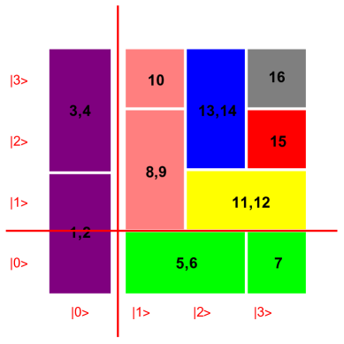
Figure 1: Representation of product states in ${\mathbf{C}}^{4}\otimes{\mathbf{C}}^{4}$. The bottom side represents Alice’s side and top left side represents Bob’s side (this is also maintained in other figures unless explicitly stated). We represent quantum states $\ket{i\pm\overline{i+1}}\ket{j}$ or, $\ket{j}\ket{i\pm\overline{i+1}}$ by rectangular tiles where $\ket{i\pm\overline{i+1}}=\frac{1}{\sqrt{2}}(\ket{i}\pm\ket{i+1}),$ for integer ‘$i$’. Each of the square tiles represent a state of the form $\ket{j}\ket{k}$. Tile indices correspond to consecutively ordered basis states of set $\mathcal{S}_{1}$, while tile colors indicate compatible measurement setups for both parties.

Consider the set $\mathcal{S}_{1}=\left\{\left|\phi_{i}\right\rangle_{AB}\right\}\in\mathbf{\mathbf{C}^{4}\otimes\mathbf{C}^{4}}$, by,

$$\mathcal{S}_{1}=\begin{Bmatrix}\mathbf{|0\rangle_{A}|{\mathcal{X}}_{01}^{\pm}\rangle_{B},}\;\mathbf{|0\rangle_{A}|{\mathcal{X}}_{23}^{\pm}\rangle_{B},}\;\mathbf{|{\mathcal{\xi}}_{12}^{\pm}\rangle_{A}|0\rangle_{B},}\;\\ \mathbf{|{\mathcal{\xi}}_{3}\rangle_{A}|0\rangle_{A},}\;\mathbf{|1\rangle_{A}|{\mathcal{X}}_{12}^{\pm}\rangle_{B},}\;\mathbf{|1\rangle_{A}|{\mathcal{X}}_{3}\rangle_{B},}\;\\ \mathbf{|{\mathcal{\xi}}_{23}^{\pm}\rangle_{A}|1\rangle_{A},}\;\mathbf{|2\rangle_{A}|{\mathcal{X}}_{23}^{\pm}\rangle_{B},}\;\\ \mathbf{|{\mathcal{\xi}}_{3}\rangle_{A}|2\rangle_{B},}\;\mathbf{|{\mathcal{\xi}}_{3}\rangle_{A}|{\mathcal{X}}_{3}\rangle_{B}}\\ \end{Bmatrix}$$ (1)

where, $|{\mathcal{\xi}}_{ij}^{\pm}\rangle_{A}=\left(\frac{|i\rangle\pm|j\rangle}{\sqrt{2}}\right)_{A},\;|{\mathcal{X}}_{ij}^{\pm}\rangle_{B}=\left(\frac{|i\rangle\pm|j\rangle}{\sqrt{2}}\right)_{B},$ and $|{\mathcal{\xi}}_{k}\rangle_{A}=|k\rangle_{A},\;|{\mathcal{X}}_{k}\rangle_{B}=|k\rangle_{B}$, see Fig. 1.

Proposition 1.

The set $\mathcal{S}_{1}$ does not possess any activable nonlocality under orthogonality-preserving LOCC, i.e., $\mathcal{H}^{\text{LOCC}}_{1}(\mathcal{S}_{1})=0.$

Proof.

Suppose Alice goes first, and let ${\mathcal{M}_{A}^{m}}^{\dagger}\mathcal{M}_{A}^{m}=[m^{a}_{ij}]_{4\times 4}$ denote any arbitrary POVM operator of Alice with outcome $m$ such that the post-measurement   states $\quad\left\{\mathcal{M}_{A}^{m}\otimes I_{B}\left|\psi_{i}\right\rangle,\right.$ $|\psi_{i}\rangle\in\mathcal{S}_{1}\}$ should be mutually orthogonal. Because $m^{a}_{ij}=0$ is necessary and sufficient for $m^{a}_{ji}=0,i<j$, we will only show $m^{a}_{ij}=0,i<j$, in the following. Then, considering the states $|0\rangle_{A}|{\mathcal{X}}_{01}^{+}\rangle_{B}$ and $|1\rangle_{A}|{\mathcal{X}}_{12}^{+}\rangle_{B},$ we know $\left\langle 0\left|{\mathcal{M}_{A}^{m}}^{\dagger}\mathcal{M}_{A}^{m}\right|1\right\rangle_{A}\left\langle 0+1|1+2\right\rangle_{B}=0.$ Thus, $m^{a}_{01}=m^{a}_{10}=0.$ In the same way, for the states $\{|0\rangle_{A}|{\mathcal{X}}_{23}^{+}\rangle_{B},|2\rangle_{A}|{\mathcal{X}}_{23}^{+}\rangle_{B}\},$ and $\{|0\rangle_{A}|{\mathcal{X}}_{23}^{+}\rangle_{B},|{\mathcal{\xi}}_{3}\rangle_{A}|2\rangle_{B}\}$, we can compute $m^{a}_{02}=m^{a}_{20}=0,m^{a}_{03}=m^{a}_{30}=0$, respectively. Similarly if we choose the states $\{|1\rangle_{A}|{\mathcal{X}}_{12}^{+}\rangle_{B},|2\rangle_{A}|{\mathcal{X}}_{23}^{+}\rangle_{B}\},$ and $\{|1\rangle_{A}|{\mathcal{X}}_{12}^{+}\rangle_{B},|{\mathcal{\xi}}_{3}\rangle_{A}|2\rangle_{B}\}$, we can see $m^{a}_{12}=m^{a}_{21}=0,m^{a}_{13}=m^{a}_{31}=0$, respectively. Now considering the states $\{|{\mathcal{\xi}}_{3}\rangle_{A}|2\rangle_{B},|2\rangle_{A}|{\mathcal{X}}_{23}^{+}\rangle_{B}\}$, we have $\left\langle 2\left|{\mathcal{M}_{A}^{m}}^{\dagger}\mathcal{M}_{A}^{m}\right|3\right\rangle_{A}\left\langle 2|2+3\right\rangle_{B}=0.$ Which imply $m^{a}_{23}=m^{a}_{32}=0.$ Therefore, ${\mathcal{M}_{A}^{m}}^{\dagger}\mathcal{M}_{A}^{m}$ is diagonal and ${\mathcal{M}_{A}^{m}}^{\dagger}\mathcal{M}_{A}^{m}=\operatorname{diag}\left(\delta_{0},\delta_{1},\delta_{2},\delta_{3}\right)$.

Now considering $|{\mathcal{\xi}}_{12}^{\pm}\rangle_{A}|0\rangle_{A},$ we get $\quad\left\langle 1+2\left|{\mathcal{M}_{A}^{m}}^{\dagger}\mathcal{M}_{A}^{m}\right|1-2\right\rangle_{A}\langle 0|0\rangle_{B}=0,\quad$ i.e., $\left\langle 1\left|{\mathcal{M}_{A}^{m}}^{\dagger}\mathcal{M}_{A}^{m}\right|1\right\rangle-\left\langle 2\left|{\mathcal{M}_{A}^{m}}^{\dagger}\mathcal{M}_{A}^{m}\right|2\right\rangle=0$. Thus, $m^{a}_{11}=m^{a}_{22}$. For the states $|{\mathcal{\xi}}_{23}^{\pm}\rangle_{A}|1\rangle_{A}$ we finally get $m^{a}_{11}=m^{a}_{22}=m^{a}_{33}.$ Therefore, ${\mathcal{M}_{A}^{m}}^{\dagger}{\mathcal{M}_{A}^{m}}$ $=\operatorname{diag}\left(\delta_{0},\gamma,\gamma,\gamma\right).$ If possible let us assume that $\delta_{0}\neq 0$ and $\gamma\neq 0$. Then after Alice’s measurement, Bob should do a nontrivial operation on his own system according to Alice’s result. We denote $\mathcal{M}_{B}^{m}$ as Bob’s operator. As we discussed above, by choosing suitable pair of states we can conclude that all the off-diagonal element of ${\mathcal{M}_{B}^{m}}^{\dagger}\mathcal{M}_{B}^{m}$ is equal to 0. Similarly for the diagonal element as we have discussed above, if we take $|0\rangle_{A}|{\mathcal{X}}_{01}^{\pm}\rangle_{B},\;|0\rangle_{A}|{\mathcal{X}}_{23}^{\pm}\rangle_{B},\;|1\rangle_{A}|{\mathcal{X}}_{12}^{\pm}\rangle_{B}$ we finally get $m^{b}_{00}=m^{b}_{11}=m^{b}_{22}=m^{b}_{33}.$ Therefore ${\mathcal{M}_{B}^{m}}^{\dagger}\mathcal{M}_{B}^{m}$ is propotional to the identity operator, i.e., ${\mathcal{M}_{B}^{m}}^{\dagger}\mathcal{M}_{B}^{m}=\lambda_{0}I$, which is trivial operator and this contradicts our assumption. So, either $\delta_{0}=0$ or $\gamma=0.$ Notice that this result also suggests that these states cannot be distinguished if Bob goes first. Now it is clear that if Alice goes first with a diagonal operator i.e., $\delta_{0}=\gamma=1$, then the above set of states cannot be distinguished. So, Alice has to do non-trivial measurement first and this only happens when any one of $\delta_{0}$, $\gamma$ not equal to zero. For that Alice only has two outcome measurement operators: $\quad{\mathcal{M}_{A}^{1}}^{\dagger}\mathcal{M}_{A}^{1}=\operatorname{diag}(1,0,0,0)$ and ${\mathcal{M}_{A}^{2}}^{\dagger}\mathcal{M}_{A}^{2}$ = $I-{\mathcal{M}_{A}^{1}}^{\dagger}\mathcal{M}_{A}^{1}$ $=\operatorname{diag}(0,1,1,1)$, see Fig. 2. If ‘$1$’ clicks, Bob is able to distinguish the left states by projecting onto $\left|0\pm 1\right\rangle$ and $\left|2\pm 3\right\rangle$. If ‘$2$’ clicks, it isolates the remaining states. It is then Bob’s turn to do measurement. Following the method we used above, we can similarly prove that Bob’s measurement must be ${\mathcal{M}_{B}^{1}}^{\dagger}\mathcal{M}_{B}^{1}=\operatorname{diag}(1,0,0,0)$ and ${\mathcal{M}_{B}^{2}}^{\dagger}\mathcal{M}_{B}^{2}$ $=\operatorname{diag}(0,1,1,1)$. The process will repeat a finite number of times and for each measurement outcomes for both parties the set $\mathcal{S}_{1}$ transforms only to a distinguishable set. This implies the fact that if the set is distinguishable (local) then for all possible nontrivial measurements, it is impossible to transform the set into an indistinguishable one. In other words, the set $\mathcal{S}_{1}$ is not activable through orthogonality-preserving LOCC. Hence we complete the proof. ∎

From the above a key point appears. The structure of the product states suggests, for local discrimination of these states local operations and two-way classical communication is necessary. Also notice that it is straightforward to generalize the structure given in Fig. 1. We just have to keep adding additional layer of titles following the pattern. Furthermore, in qubit-qudit case such a class is quite obvious bandhyopadhyay201 . Clearly, the two-qudit construction given in this paper is nontrivial.

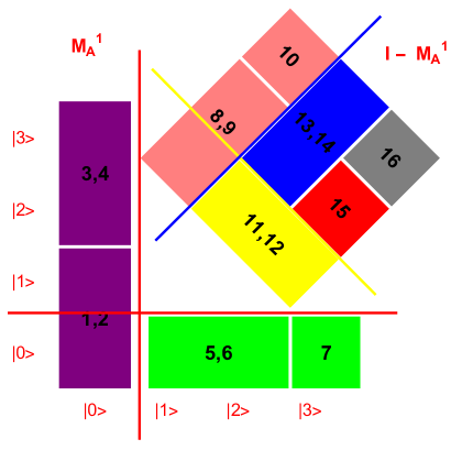
Figure 2: Representation of product states in ${\mathbb{C}}^{4}\otimes{\mathbb{C}}^{4}$. Tile indices correspond to consecutively ordered basis states of set $\mathcal{S}_{1}$, while tile colors indicate compatible measurement setups for both parties. $\mbox{M}_{i}^{j}={\mathcal{M}_{i}^{j}}^{\dagger}\mathcal{M}_{i}^{j}$; $i=\mbox{A, B}$, $j=1,2$ (this is also maintained in other figures unless explicitly stated).

For bipartite systems the variation with respect to hidden kind of nonlocality is very limited as $k$ can have only one value ($k=1$). So, there are only two types of structures, one is activable and the other is non-activable. Both classes are weaker in the sense of nonlocality because they are not locally indistinguishable class after all.

However, multipartite Hilbert spaces provide some interesting results which cannot be seen for bipartite Hilbert spaces. More generally, for the task of activation of nonlocality the multipartite Hilbert space provides some broader view than bipartite cases. For example, in the tripartite scenario there exists a set of states, $\mathcal{S}$ which is not activable when all three parties are spatially separated, i.e., $\mathcal{H}^{\text{LOCC}}_{1}(\mathcal{S})=0.$, but the same set of states might be activable when two parties perform some joint operation(s), i.e., $\mathcal{H}^{\text{LOCC}}_{2}(\mathcal{S})$ may not be zero subrata2024 . Consequently, a question arises: Is it feasible to construct a tripartite set for which the activation of nonlocality by LOCC is precluded across every bipartition? Such a class would, in essence, constitute the ‘worst case’ from the perspective of non-locality activation. The subsequent findings furnish appropriate support for this aforementioned concept. Consider the set $\mathcal{S}_{2}=\left\{\left|\phi_{i}\right\rangle_{AB}\right\}\in\mathbf{\mathbf{C}^{4}\otimes\mathbf{C}^{2}\otimes\mathbf{C}^{2}}$, given by,

$$\mathcal{S}_{2}=\begin{Bmatrix}\mathbf{|\xi_{0}\rangle_{A}|{\mathcal{X}_{0}}\rangle_{B}|{\mathcal{Y}}_{01}^{\pm}\rangle_{C},}\;\mathbf{|\xi_{0}\rangle_{A}|{\mathcal{X}_{1}}\rangle_{B}|{\mathcal{Y}}_{01}^{\pm}\rangle_{C},}\;\\ \mathbf{|{\mathcal{\xi}}_{12}^{\pm}\rangle_{A}|\mathcal{X}_{0}\rangle_{B}|\mathcal{Y}_{0}\rangle_{C},}\;\mathbf{|{\mathcal{\xi}}_{3}\rangle_{A}|\mathcal{X}_{0}\rangle_{B}|\mathcal{Y}_{0}\rangle_{C},}\;\\ \mathbf{|\xi_{1}\rangle_{A}|{\mathcal{X}}_{1}\rangle_{B}|{\mathcal{Y}}_{0}\rangle_{C},}\;\mathbf{|{\mathcal{\xi}}_{3}\rangle_{A}|\mathcal{X}_{1}\rangle_{B}|\mathcal{Y}_{0}\rangle_{C}}\\ \mathbf{|\xi_{1}\rangle_{A}|{\mathcal{X}}_{01}^{\pm}\rangle_{B}|\mathcal{Y}_{1}\rangle_{C},}\;\mathbf{|{\mathcal{\xi}}_{23}^{\pm}\rangle_{A}|\mathcal{X}_{0}\rangle_{B}|\mathcal{Y}_{1}\rangle_{C},}\;\\ \mathbf{|{\mathcal{\xi}}_{3}\rangle_{A}|\mathcal{X}_{1}\rangle_{B}|\mathcal{Y}_{1}\rangle_{C},}\;\end{Bmatrix}$$ (2)

where, $|{\mathcal{\xi}}_{ij}^{\pm}\rangle_{A}=\left(\frac{|i\rangle\pm|j\rangle}{\sqrt{2}}\right)_{A},\;|{\mathcal{X}}_{ij}^{\pm}\rangle_{B}=\left(\frac{|i\rangle\pm|j\rangle}{\sqrt{2}}\right)_{B},\;$
$|{\mathcal{Y}}_{ij}^{\pm}\rangle_{C}=\left(\frac{|i\rangle\pm|j\rangle}{\sqrt{2}}\right)_{C}$ and $|{\mathcal{\xi}}_{k}\rangle_{A}=|k\rangle_{A},\;|{\mathcal{X}}_{k}\rangle_{B}=|k\rangle_{B}$
$|{\mathcal{Y}}_{k}\rangle_{C}=|k\rangle_{C}$.

Proposition 2.

The set $\mathcal{S}_{2}$ does not possess any activable nonlocality in tripartition $A|B|C$ as well as in all bipartition under orthogonality-preserving LOCC. i.e., $(i)\;\mathcal{H}^{\text{LOCC}}_{1}(\mathcal{S}_{2})=0$ and $(ii)\;\mathcal{H}^{\text{LOCC}}_{2}(\mathcal{S}_{2})=0.$

Proof.

(i) We begin by noting that given any multipartite set, if it does not contain any activable nonlocality across all bipartitions then it becomes obvious that the set also does not contain any activable nonlocality in multi-partitions. This is because in bipartitions the operations are stronger than that of the multi-partitions. For example, in our context if we consider a bipartition then, two parties can perform joint measurements but in a tripartition such a possibility is absent. Clearly, the operations in bipartitions can be much stronger than that of a tripartition. Thus, we concentrate only on proving the second part of the proposition.

(ii) We need to prove that $\mathcal{S}_{2}$ is not activable in all bipartitions. First, we consider the case A|BC. In A|BC, the states belong to a $\mathbf{\mathbf{C}^{4}\otimes\mathbf{C}^{4}}$ Hilbert space and they have the same forms as the states of the set $\mathcal{S}_{1}$. So, by Proposition 1, the set of states $\mathcal{S}_{2}$ is non-activable in A|BC bipartition.

For the bipartitions B|AC and C|AB, the states of the set $\mathcal{S}_{2}$ belong to $\mathbf{\mathbf{C}^{2}\otimes\mathbf{C}^{8}}$. Now, it is known that a set of product states in $\mathbf{\mathbf{C}^{2}\otimes\mathbf{C}^{n}}$ is always locally distinguishable BennettUPB1999 . Moreover, LOCC is not sufficient to create entanglement from product states. So, it is impossible to activate nonlocality from the states of the set $\mathcal{S}_{2}$ in B|AC and C|AB bipartitions. Hence $\mathcal{H}^{\text{LOCC}}_{2}(\mathcal{S}_{2})=0.$ ∎

Remark 3.

Let us not concentrate on the particular structure of tripartite product states, given in (2). Instead, we consider any tripartite orthogonal product states in $\mathbf{\mathbf{C}^{4}\otimes\mathbf{C}^{2}\otimes\mathbf{C}^{2}}$ such that these states mimic the similar forms like the states of (1) in $\mathbf{\mathbf{C}^{4}\otimes\mathbf{C}^{4}}$ bipartition. Then, from the aforesaid proof technique it depicts that for such a set the activable nonlocality is 0 across all bipartitions.

In a three-qubit system, it is observed that all sets of orthogonal product states are non-activable across every bipartition. This deduction stems directly from the established fact that, in qubit-qudit scenarios, orthogonal product states consistently exhibit local distinguishability BennettUPB1999 . Consequently, from this standpoint, our proposed higher-dimensional construction presents a point of particular interest.

Next, we want to discuss about a hierarchy among the multipartite locally distinguishable sets. For this purpose, we first consider the bipartite set $\mathcal{S}_{3}=\left\{\left|\phi_{i}\right\rangle_{AB}\right\}_{i=1}^{10}\in\mathbf{\mathbf{C}^{6}\otimes\mathbf{C}^{6}}$, where

$$\begin{aligned} &\left|\phi_{1}\right\rangle_{AB}=|\mathbf{0}\rangle_{A}|\mathbf{0}-\mathbf{1}+\mathbf{4}-\mathbf{5}\rangle_{B}\\ &\left|\phi_{2}\right\rangle_{AB}=|\mathbf{2}\rangle_{A}|\mathbf{1}-\mathbf{2}+\mathbf{5}-\mathbf{3}\rangle_{B}\\ &\left|\phi_{3}\right\rangle_{AB}=|\mathbf{1-2}\rangle_{A}|\mathbf{0}-\mathbf{4}\rangle_{B}\\ &\left|\phi_{4}\right\rangle_{AB}=|\mathbf{0-1}\rangle_{A}|\mathbf{2}-\mathbf{3}\rangle_{B}\\ &\left|\phi_{5}\right\rangle_{AB}=|\mathbf{0+1+2}\rangle_{A}|\mathbf{0}+\mathbf{1}+\mathbf{2}+\mathbf{3}+\mathbf{4}+\mathbf{5}\rangle_{B}\\ &\left|\phi_{6}\right\rangle_{AB}=|\mathbf{3}\rangle_{A}|\mathbf{0}-\mathbf{1}+\mathbf{4}-\mathbf{5}\rangle_{B}\\ &\left|\phi_{7}\right\rangle_{AB}=|\mathbf{5}\rangle_{A}|\mathbf{1}-\mathbf{2}+\mathbf{5}-\mathbf{3}\rangle_{B}\\ &\left|\phi_{8}\right\rangle_{AB}=|\mathbf{4-5}\rangle_{A}|\mathbf{0}-\mathbf{4}\rangle_{B}\\ &\left|\phi_{9}\right\rangle_{AB}=|\mathbf{3-4}\rangle_{A}|\mathbf{2}-\mathbf{3}\rangle_{B}\\ &\left|\phi_{10}\right\rangle_{AB}=|\mathbf{3+4+5}\rangle_{A}|\mathbf{0}+\mathbf{1}+\mathbf{2}+\mathbf{3}+\mathbf{4}+\mathbf{5}\rangle_{B}\end{aligned}$$ (3)

It is quite straightforward to show that the set $\mathcal{S}_{3}$ considered above is free from local redundancy bandhyopadhyay201 ; Li2022 ; subrata2024 . Here, Bob’s system can be considered to be the composition of qubit and qutrit subsystems,

$$|\mathbf{0}\rangle_{B} :=|00\rangle_{b_{1}b_{2}}, |\mathbf{1}\rangle_{B}:=|01\rangle_{b_{1}b_{2}},$$

$$|\mathbf{2}\rangle_{B} :=|02\rangle_{b_{1}b_{2}}, |\mathbf{3}\rangle_{B}:=|10\rangle_{b_{1}b_{2}},$$

$$\left|\mathbf{4}_{B}\right\rangle :=|11\rangle_{b_{1}b_{2}}, |\mathbf{5}\rangle_{B}:=|12\rangle_{b_{1}b_{2}}.$$

Take two states, $\left|\phi_{3}\right\rangle_{AB}$ and $\left|\phi_{4}\right\rangle_{AB}$. When any of the subparts (qubit or qutrit) of Bob’s system for both states is discarded the reduced states will be nonorthogonal. Similar things happen for Alice also. This implies the set $\mathcal{S}_{3}$ is free from local redundancy.

Now we will show that the set $\mathcal{S}_{3}$ is locally distinguishable. The players can avail the following discrimination protocol. First Bob performs a measurement:

$$\mathcal{M}_{B}\equiv \{\mathcal{M}_{B}^{1}:=P\left[|\mathbf{0}-\mathbf{4}\rangle_{B}\right],\mathcal{M}_{B}^{2}:=P\left[|\mathbf{2}-\mathbf{3}\rangle_{B}\right],$$

$$\mathcal{M}_{B}^{3}:=P\left[\ket{\mathbf{0}+\mathbf{1}+\mathbf{2}+\mathbf{3}+\mathbf{4}+\mathbf{5}}_{B}\right],$$

$$\mathcal{M}_{B}^{4}:=\mathbb{I}-\left(\mathcal{M}_{B}^{1}+\mathcal{M}_{B}^{2}+\mathcal{M}_{B}^{3}\right)\}.$$

Here, $P\left[|\cdot\rangle\right]:=$ $|\cdot\rangle\langle\cdot|_{\mathcal{P}}$, and $\mathcal{P}$ denotes the party. When $\mathcal{M}_{B}^{1}$ clicks, the given state must be $\left|\phi_{3}\right\rangle$ and $\left|\phi_{8}\right\rangle$, which can be distinguished by Alice, projecting onto $|\mathbf{1-2}\rangle$ and $|\mathbf{4-5}\rangle$. Similarly, for the click $\mathcal{M}_{B}^{2}$, the states are $\left|\phi_{4}\right\rangle$ and $\left|\phi_{9}\right\rangle$, which can be distinguished by Alice, projecting onto $|\mathbf{0-1}\rangle$ and $|\mathbf{3-4}\rangle$. Also for the outcome $\mathcal{M}_{B}^{3}$ the isolated states are $\left|\phi_{5}\right\rangle$ and $\left|\phi_{10}\right\rangle$, which can be distinguished by Alice, projecting onto $|\mathbf{0+1+2}\rangle$ and $|\mathbf{3+4+5}\rangle$. Whenever $\mathcal{M}_{B}^{4}$ clicks the given state can be $\left|\phi_{1}\right\rangle$, $\left|\phi_{2}\right\rangle$, $\left|\phi_{6}\right\rangle$ and $\left|\phi_{7}\right\rangle$. However, in that case, Alice can perform a measurement

$$\mathcal{M}_{A} \equiv\left\{\mathcal{M}_{A}^{1}:=\right.P\left[|\mathbf{0}\rangle_{A}\right],\mathcal{M}_{A}^{2}:=P\left[|\mathbf{2}\rangle_{A}\right],$$

$$\mathcal{M}_{A}^{3}:=P[\ket{\mathbf{3}}_{A}],\mathcal{M}_{A}^{4}:=\mathbb{I}-\left(\mathcal{M}_{A}^{1}+\mathcal{M}_{A}^{2}+\mathcal{M}_{A}^{3}\right)\},$$

to distinguish between these four states. This concludes the local discrimination protocol for the set $\mathcal{S}_{3}$. In the following, we will demonstrate a protocol to activate nonlocality without entanglement from this set.

Proposition 4.

The set $\mathcal{S}_{3}$ is a locally distinguishable set and can be transformed deterministically to a locally irreducible set via orthogonality-preserving LOCC.

Proof.

Consider that Bob performs a local measurement

$$\mathcal{K}_{B} \equiv\left\{\mathcal{K}^{B}_{1}:=P\left[(|\mathbf{0}\rangle,|\mathbf{1}\rangle,|\mathbf{2}\rangle)_{B}\right],\mathcal{K}^{B}_{2}:=P\left[(|\mathbf{3}\rangle,|\mathbf{4}\rangle,|\mathbf{5}\rangle)_{B}\right]\right\},$$

$$P\left[(|i\rangle,|j\rangle,\dots)_{\mathcal{P}}\right]=\left[(|i\rangle\langle i|+|j\rangle\langle j|+\dots)_{\mathcal{P}}\right],$$

$\mathcal{P}$ stands for party. If $\mathcal{K}^{B}_{1}$ clicks, they end up with,

$$\left\{\begin{array}[]{c}|\mathbf{0}\rangle_{A}|\mathbf{0}-\mathbf{1}\rangle_{B},|\mathbf{2}\rangle_{A}|\mathbf{1}-\mathbf{2}\rangle_{B},\\ |\mathbf{1-2}\rangle_{A}|\mathbf{0}\rangle_{B},|\mathbf{0-1}\rangle_{A}|\mathbf{2}\rangle_{B},\\ |\mathbf{0+1+2}\rangle_{A}|\mathbf{0}+\mathbf{1}+\mathbf{2}\rangle_{B},\\ |\mathbf{3}\rangle_{A}|\mathbf{0}-\mathbf{1}\rangle_{B},|\mathbf{5}\rangle_{A}|\mathbf{1}-\mathbf{2}\rangle_{B},\\ |\mathbf{4-5}\rangle_{A}|\mathbf{0}\rangle_{B},|\mathbf{3-4}\rangle_{A}|\mathbf{2}\rangle_{B},\\ |\mathbf{3+4+5}\rangle_{A}|\mathbf{0}+\mathbf{1}+\mathbf{2}\rangle_{B}\end{array}\right\}$$

After that Alice makes measurement $\mathcal{K}_{A}\equiv\left\{\mathcal{K}^{A}_{1}:=P\left[(|\mathbf{0}\rangle,|\mathbf{1}\rangle,|\mathbf{2}\rangle)_{A}\right],\mathcal{K}^{A}_{2}:=\right.$ $\left.P\left[(|\mathbf{3}\rangle,|\mathbf{4}\rangle,|\mathbf{5}\rangle)_{A}\right]\right\}$. If $\mathcal{K}^{A}_{1}$ occurs, it gives,

$$\left\{\begin{array}[]{c}|\mathbf{0}\rangle_{A}|\mathbf{0}-\mathbf{1}\rangle_{B},|\mathbf{2}\rangle_{A}|\mathbf{1}-\mathbf{2}\rangle_{B},\\ |\mathbf{1-2}\rangle_{A}|\mathbf{0}\rangle_{B},|\mathbf{0-1}\rangle_{A}|\mathbf{2}\rangle_{B},\\ |\mathbf{0+1+2}\rangle_{A}|\mathbf{0}+\mathbf{1}+\mathbf{2}\rangle_{B}\end{array}\right\}$$

which is a locally irreducible set BennettUPB1999 . If $\mathcal{K}^{A}_{2}$ occurs, it also gives a locally irreducible set,

$$\left\{\begin{array}[]{c}|\mathbf{3}\rangle_{A}|\mathbf{0}-\mathbf{1}\rangle_{B},|\mathbf{5}\rangle_{A}|\mathbf{1}-\mathbf{2}\rangle_{B},\\ |\mathbf{4-5}\rangle_{A}|\mathbf{0}\rangle_{B},|\mathbf{3-4}\rangle_{A}|\mathbf{2}\rangle_{B},\\ |\mathbf{3+4+5}\rangle_{A}|\mathbf{0}+\mathbf{1}+\mathbf{2}\rangle_{B}\end{array}\right\}$$

On the other hand, if Bob gets $\mathcal{K}^{B}_{2}$, they are then left with the following states,

$$\left\{\begin{array}[]{c}|\mathbf{0}\rangle_{A}|\mathbf{4}-\mathbf{5}\rangle_{B},|\mathbf{2}\rangle_{A}|\mathbf{5}-\mathbf{3}\rangle_{B},\\ |\mathbf{1-2}\rangle_{A}|\mathbf{4}\rangle_{B},|\mathbf{0-1}\rangle_{A}|\mathbf{3}\rangle_{B},\\ |\mathbf{0+1+2}\rangle_{A}|\mathbf{3}+\mathbf{4}+\mathbf{5}\rangle_{B},\\ |\mathbf{3}\rangle_{A}|\mathbf{4}-\mathbf{5}\rangle_{B},|\mathbf{5}\rangle_{A}|\mathbf{5}-\mathbf{3}\rangle_{B},\\ |\mathbf{4-5}\rangle_{A}|\mathbf{4}\rangle_{B},|\mathbf{3-4}\rangle_{A}|\mathbf{3}\rangle_{B},\\ |\mathbf{3+4+5}\rangle_{A}|\mathbf{3}+\mathbf{4}+\mathbf{5}\rangle_{B}\end{array}\right\}$$

After that Alice makes a measurement

$$\mathcal{K}_{A} \equiv\left\{\mathcal{K}^{A}_{1}:=P\left[(|\mathbf{0}\rangle,|\mathbf{1}\rangle,|\mathbf{2}\rangle)_{A}\right]\right.,$$

$$\left.\mathcal{K}^{A}_{2}:=P\left[(|\mathbf{3}\rangle,|\mathbf{4}\rangle,|\mathbf{5}\rangle)_{A}\right]\right\}.$$

If $\mathcal{K}^{A}_{1}$ occurs, it gives,

$$\left\{\begin{array}[]{c}|\mathbf{0}\rangle_{A}|\mathbf{4}-\mathbf{5}\rangle_{B},|\mathbf{2}\rangle_{A}|\mathbf{5}-\mathbf{3}\rangle_{B},\\ |\mathbf{1-2}\rangle_{A}|\mathbf{4}\rangle_{B},|\mathbf{0-1}\rangle_{A}|\mathbf{3}\rangle_{B},\\ |\mathbf{0+1+2}\rangle_{A}|\mathbf{3}+\mathbf{4}+\mathbf{5}\rangle_{B}\end{array}\right\}$$

which is a locally irreducible set. If $\mathcal{K}^{A}_{2}$ occurs, it also gives a locally irreducible set,

$$\left\{\begin{array}[]{c}|\mathbf{3}\rangle_{A}|\mathbf{4}-\mathbf{5}\rangle_{B},|\mathbf{5}\rangle_{A}|\mathbf{5}-\mathbf{3}\rangle_{B},\\ |\mathbf{4-5}\rangle_{A}|\mathbf{4}\rangle_{B},|\mathbf{3-4}\rangle_{A}|\mathbf{3}\rangle_{B},\\ |\mathbf{3+4+5}\rangle_{A}|\mathbf{3}+\mathbf{4}+\mathbf{5}\rangle_{B}\end{array}\right\}$$

It is evident that, for each instance of Alice’s measurement, specified by the set $\{\mathcal{K}^{A}_{1},\;\mathcal{K}^{A}_{2}\}$; the five post-measurement states, contingent upon $\mathcal{K}^{B}_{1}$ clicking, yield the celebrated unextendable product basis (UPB) BennettPB1999 ; BennettUPB1999 in $\mathbf{C^{3}\otimes C^{3}}$. Also, the post-measurement states for each case of Alice’s measurement $\mathcal{K}^{A}_{1},\;\mathcal{K}^{A}_{2}$ when $\mathcal{K}^{B}_{2}$ clicks form the same UPB. See Fig. 3. It has been well established that UPB is locally indistinguishable Divincinzo ; BennettUPB1999 . So, the set $\mathcal{S}_{3}$ is activable by orthogonality-preserving LOCC. Hence, this completes the proof. ∎

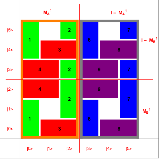
Figure 3: Tiling diagram for the states in $\mathbf{\mathcal{S}_{3}}$. The outlined region indicates the support of Alice’s and Bob’s measurement outcomes, resulting in post-measurement states, contained in a UPB subspace. $\mbox{M}_{i}^{j}={\mathcal{K}_{j}^{i}}$; $i=\mbox{A, B}$, $j=1,2$

Towards a hierarchy: We consider the set $\mathcal{S}_{4}=\left\{\left|\phi_{i}\right\rangle_{AB}\otimes\left|0\right\rangle_{C},\left|\phi_{i}\right\rangle_{AB}\otimes\left|1\right\rangle_{C}\right\}_{i=1}^{10}\in\mathbf{C}^{6}\otimes\mathbf{C}^{6}\otimes\mathbf{C}^{2}$, where $\left\{\left|\phi_{i}\right\rangle_{AB}\right\}_{i=1}^{10}=\mathcal{S}_{3}$. Now, consider all bipartitions of the tripartite system. For the bipartition $AB|C$, the total Hilbert space is $\mathbf{C}^{2}\otimes\mathbf{C}^{36}$, and due to the limited dimension of subsystem $C$, the set remains non-activable in this cut bandhyopadhyay201 . However, for the bipartitions $A|BC$ and $B|AC$, the set becomes activable. This follows directly from Proposition 3.

Remark 5.

Let us now highlight the contrasting structures of the sets $\mathcal{S}_{2}$ and $\mathcal{S}_{4}$. The set $\mathcal{S}_{2}$ is a tripartite ensemble of orthogonal quantum states that is initially locally distinguishable and remains non-activable in all bipartitions. In contrast, the set $\mathcal{S}_{4}$ is activable in certain bipartitions (but not in every bipartition). This structural difference reveals a clear separation in the degrees of hidden nonlocality for $\mathcal{S}_{2}$ and $\mathcal{S}_{4}$.

So far, we have discussed about the product states only. Nevertheless, in the following, we include entangled states into our discussions.

IV Non-activable entangled states

Here we consider several sets that are local and non-activable by LOCC, i.e., $\mathcal{H}^{\text{LOCC}}_{1}(\mathcal{S}_{j})=0$, for different sets $\mathcal{S}_{j}$. $|^{\theta}\mathcal{W}_{ij,kl}^{\pm}\rangle_{AB}=|\theta\rangle_{A}|{\mathcal{X}}_{ij}^{\pm}\rangle_{B}+|\bar{(\theta+2)}\rangle_{A}|{\mathcal{X}}_{kl}^{\pm}\rangle_{B},\;$ and $|^{\theta}\mathcal{W}_{ij,m}^{\pm}\rangle_{AB}=|\theta\rangle_{A}|{\mathcal{X}}_{ij}^{\pm}\rangle_{B}+|\bar{(\theta+2)}\rangle_{A}|{\mathcal{X}}_{m}\rangle_{B},\;$ also $|^{\theta}\mathcal{\bar{W}}_{ij,kl}^{\pm}\rangle_{AB}=|{\mathcal{\xi}}_{ij}^{\pm}\rangle_{A}|\theta\rangle_{B}+|{\mathcal{\xi}}_{kl}^{\pm}\rangle_{A}|\bar{(\theta+2)}\rangle_{B},\;$ and $|^{\theta}\mathcal{\bar{W}}_{ij,m}^{\pm}\rangle_{AB}=|{\mathcal{\xi}}_{ij}^{\pm}\rangle_{A}|\theta\rangle_{B}+|{\mathcal{\xi}}_{m}\rangle_{A}|\bar{(\theta+2)}\rangle_{B},\;$, for $\theta=0,1$ and $\bar{(\theta+2)}$ denotes $(\theta+2)$ modulo d. Here we consider the set $\mathcal{S}_{5}=\left\{\left|\phi_{i}\right\rangle_{AB}\right\}\in\mathbf{\mathbf{C}^{4}\otimes\mathbf{C}^{4}}$, which contains product states as well as entangled states. The set is given by-

$$\mathcal{S}_{5}=\begin{Bmatrix}\mathbf{|^{0}\mathcal{W}_{01,23}^{\pm}\rangle_{AB},}\;\mathbf{|0\rangle_{A}|{\mathcal{X}}_{23}^{\pm}\rangle_{B},}\;\mathbf{|^{0}\mathcal{\bar{W}}_{12,3}^{+}\rangle_{AB},}\;\\ \mathbf{|{\mathcal{\xi}}_{12}^{-}\rangle_{A}|0\rangle_{B},}\;\mathbf{|{\mathcal{\xi}}_{3}\rangle_{A}|0\rangle_{B},}\;\mathbf{|^{1}\mathcal{W}_{12,3}^{+}\rangle_{AB},}\;\\ \mathbf{|1\rangle_{A}|{\mathcal{X}}_{12}^{-}\rangle_{B},}\;\mathbf{|1\rangle_{A}|{\mathcal{X}}_{3}\rangle_{B},}\;\mathbf{|{\mathcal{\xi}}_{23}^{\pm}\rangle_{A}|1\rangle_{B}}\end{Bmatrix}$$ (4)

Proposition 6.

The set $\mathcal{S}_{5}$ does not possess any activable nonlocality under orthogonality-preserving LOCC. That is, its hidden nonlocality $\mathcal{H}^{\text{LOCC}}_{1}(\mathcal{S}_{5})=0.$

Proof.

Here the states of (4) are nothing but the superposition of states of (1). The only difference between them is that one contains entangled states and the other contains only product states. So, the outline of the proof is similar to that of the Proposition 1. Without loss of generality, let us assume that Alice goes first. Considering the states $|0\rangle_{A}|{\mathcal{X}}_{23}^{+}\rangle_{B},\;|1\rangle_{A}|{\mathcal{X}}_{3}\rangle_{B},$ we have $\left\langle 0\left|{\mathcal{M}_{A}^{m}}^{\dagger}\mathcal{M}_{A}^{m}\right|1\right\rangle_{A}\left\langle 2+3|3\right\rangle_{B}=0,$ which implies that , $m^{a}_{01}=m^{a}_{10}=0.$

In the same way, for the states $|^{0}\mathcal{W}_{01,23}^{+}\rangle_{AB},\;|0\rangle_{A}|{\mathcal{X}}_{23}^{\pm}\rangle_{B}$ and $|^{1}\mathcal{W}_{12,3}^{+}\rangle_{AB}$, we have $m^{a}_{02}=m^{a}_{20}=0,m^{a}_{03}=m^{a}_{30}=0$, respectively. Similarly, by choosing appropriate pair of states we get $m^{a}_{ij}=m^{a}_{ji}=0,\forall i\neq j$. Therefore, ${\mathcal{M}_{A}^{m}}^{\dagger}\mathcal{M}_{A}^{m}$ is diagonal and ${\mathcal{M}_{A}^{m}}^{\dagger}\mathcal{M}_{A}^{m}$ $=\operatorname{diag}\left(\delta_{0},\delta_{1},\delta_{2},\delta_{3}\right).$

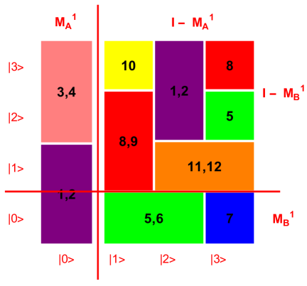
Figure 4: Tile structure of the states in ${\mathbf{C}}^{4}\otimes{\mathbf{C}}^{4}$, given in (4). The indices of the tiles comes from the order the states of $\mathcal{S}_{5}$ consecutively. The color of the tiles represents the possibility of measurement setup for both the parties.

Next considering $|^{0}\mathcal{\bar{W}}_{12,3}^{+}\rangle_{AB}$ and $|{\mathcal{\xi}}_{12}^{-}\rangle_{A}|0\rangle_{B},$ we get $\left\langle 1+2\left|{\mathcal{M}_{A}^{m}}^{\dagger}\mathcal{M}_{A}^{m}\right|1-2\right\rangle_{A}\langle 0|0\rangle_{B}=0,$ i.e., $\left\langle 1\left|{\mathcal{M}_{A}^{m}}^{\dagger}\mathcal{M}_{A}^{m}\right|1\right\rangle-\left\langle 2\left|{\mathcal{M}_{A}^{m}}^{\dagger}\mathcal{M}_{A}^{m}\right|2\right\rangle=0$. Thus, $m^{a}_{11}=m^{a}_{22}$. By using the states $|{\mathcal{\xi}}_{23}^{\pm}\rangle_{A}|1\rangle_{B},$ we finally get $m^{a}_{11}=m^{a}_{22}=m^{a}_{33}.$ Therefore, ${\mathcal{M}_{A}^{m}}^{\dagger}\mathcal{M}_{A}^{m}$ $=\operatorname{diag}\left(\delta_{0},\gamma,\gamma,\gamma\right).$ If possible, let us assume that $\delta_{0}\neq 0$ and $\gamma\neq 0$. Then after Alice’s measurement, Bob should do a nontrivial operation on his own subsystem according to Alice’s result. We denote $\mathcal{M}_{B}^{m}\;(where,\;{\mathcal{M}_{B}^{m}}^{\dagger}\mathcal{M}_{B}^{m}=(m^{b}_{ij})_{4\times 4})$ as Bob’s operator. As we have discussed above, by choosing suitable pair of states we can conclude that all the off-diagonal elements of ${\mathcal{M}_{B}^{m}}^{\dagger}\mathcal{M}_{B}^{m}$ are equal to $0$. Similarly, for the diagonal elements as we have discussed above, if we consider the states $|^{0}\mathcal{W}_{01,23}^{\pm}\rangle_{AB},\;|0\rangle_{A}|{\mathcal{X}}_{23}^{\pm}\rangle_{B},\;|{\mathcal{\xi}}_{3}\rangle_{A}|0\rangle_{A}$ and $|1\rangle_{A}|{\mathcal{X}}_{12}^{-}\rangle_{B}$, we finally get, $m^{b}_{00}=m^{b}_{11}=m^{b}_{22}=m^{b}_{33}.$ Therefore, ${\mathcal{M}_{B}^{m}}^{\dagger}\mathcal{M}_{B}^{m}$ is proportional to the identity operator, i.e., ${\mathcal{M}_{B}^{m}}^{\dagger}\mathcal{M}_{B}^{m}=\lambda_{0}I$, which is the trivial operator and this contradicts our assumption that $\mathcal{S}_{5}$ is initially local. So, either $\delta_{0}=0$ or $\gamma=0.$ Notice that this result also suggests us that these states cannot be distinguished locally if Bob goes first. Now it is clear that if Alice goes first with a diagonal operator, i.e., $\delta_{0}=\gamma=1$, then the above set of states cannot be distinguished. So, Alice has to do non-trivial measurement first and this only happens when any one of $\delta_{0}$, $\gamma$ is not equal to zero. For that Alice only has two outcome measurement operators: $\quad{\mathcal{M}_{A}^{1}}^{\dagger}\mathcal{M}_{A}^{1}=\operatorname{diag}(1,0,\ldots,0)$ and ${\mathcal{M}_{A}^{2}}^{\dagger}\mathcal{M}_{A}^{2}$ $=\operatorname{diag}(0,1,1\ldots,1)$, see Fig. 4. If the outcome ‘$1$’ click, Bob is able to distinguish the remaining states by projecting onto $\left|0\pm 1\right\rangle$ and $\left|2\pm 3\right\rangle$. If the measurement outcome is ‘$2$’, it will isolate the remaining states. It is then Bob’s turn to do measurement. Following the method we used above, we can similarly prove that Bob’s measurement must be ${\mathcal{M}_{B}^{1}}^{\dagger}\mathcal{M}_{B}^{1}=\operatorname{diag}(1,0,0,0)$ and ${\mathcal{M}_{B}^{2}}^{\dagger}\mathcal{M}_{B}^{2}$ $=\operatorname{diag}(0,1,1,1)$. The process will repeat a finite number of times, and for each measurement outcome for both parties, the set $\mathcal{S}_{3}$ transforms only to a distinguishable set. This implies the fact that, if the set is distinguishable (local), then for all possible nontrivial measurements, it is impossible to transform the set into an indistinguishable one. That is in other words, the set $\mathcal{S}_{5}$ is not activable through orthogonality-preserving LOCC. This completes the proof. ∎

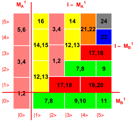
Figure 5: Tiles representation of states in $\mathbf{\mathbf{C}^{6}\otimes\mathbf{C}^{6}}$, indexed by states of $\mathcal{S}_{6}$ in order and colored according to the possibility of simultaneous local measurements by both parties.

It is not very difficult to construct the set $\mathcal{S}_{5}$ in arbitrary higher dimensions from its hereditary symmetry. For the case of higher dimensions, the only change will be the number of classical rounds required for discrimination task. Eventually for higher dimensions, the LOCC round numbers drastically increase for the corresponding tasks, but for each round the post-measurement states becomes distinguishable (local). Also, one can find the trade off between the dimensions of the systems and the corresponding required LOCC round number for the discrimination tasks. Now, consider the set $\mathcal{S}_{6}=\left\{\left|\phi_{i}\right\rangle_{AB}\right\}\in\mathbf{\mathbf{C}^{6}\otimes\mathbf{C}^{6}}$, by

$$\mathcal{S}_{6}=\begin{Bmatrix}\mathbf{|^{0}\mathcal{W}_{01,23}^{\pm}\rangle_{AB},}\;\mathbf{|^{0}\mathcal{W}_{23,45}^{\pm}\rangle_{AB},}\;\mathbf{|0\rangle_{A}|{\mathcal{X}}_{45}^{\pm}\rangle_{B},}\;\\ \mathbf{|^{0}\mathcal{\bar{W}}_{12,34}^{\pm}\rangle_{AB},}\;\mathbf{|^{0}\mathcal{\bar{W}}_{34,5}^{+}\rangle_{AB},}\;\mathbf{|{\mathcal{\xi}}_{34}^{-}\rangle_{A}|0\rangle_{B},}\;\\ \mathbf{|{\mathcal{\xi}}_{5}\rangle_{A}|0\rangle_{A},}\;\mathbf{|^{1}\mathcal{W}_{12,34}^{\pm}\rangle_{AB},}\;\mathbf{|^{1}\mathcal{W}_{34,5}^{+}\rangle_{AB},}\;\\ \mathbf{|1\rangle_{A}|{\mathcal{X}}_{34}^{-}\rangle_{B},}\;\mathbf{|1\rangle_{A}|{\mathcal{X}}_{5}\rangle_{B},}\;\mathbf{|^{1}\mathcal{\bar{W}}_{23,45}^{\pm}\rangle_{AB},}\;\\ \mathbf{|{\mathcal{\xi}}_{45}^{\pm}\rangle_{A}|0\rangle_{B},}\mathbf{|4\rangle_{A}|{\mathcal{X}}_{45}^{\pm}\rangle_{B},\;}\mathbf{|{\mathcal{\xi}}_{5}\rangle_{A}|4\rangle_{A},}\;\\ \mathbf{|\xi_{5}\rangle_{A}|{\mathcal{X}}_{5}\rangle_{B}}\end{Bmatrix}$$ (5)

By the similar technique as given for (4), it is possible to show that the set $\mathcal{S}_{6}$ does not possess any activable nonlocality under orthogonality-preserving LOCC, i.e., $\mathcal{H}^{\text{LOCC}}_{1}(\mathcal{S}_{6})=0$. See Fig. 5. Here we now discuss the following hierarchy. The sets of states considered in (5) and (3) are equally local when considered with respect to perfect discrimination by LOCC, as in both cases, the sets are perfectly distinguishable by LOCC. But the consideration of hidden nonlocality provides us the privilege to put a hierarchy among the sets. Precisely, we can claim that the sets of (5) are more local compared to those of (3), because the latter class contains hidden nonlocality while for the former case there is no hidden nonlocality though the set of (5) contains entangled states but the set of (3) does not.

V Conclusion

In this manuscript, we have presented structures for locally distinguishable product states and entangled states such that they cannot be transformed to a locally indistinguishable set under orthogonality-preserving LOCC. Furthermore, we have constructed sets of multipartite states which is not activable in any bipartition. In other words, such locally distinguishable sets cannot be transformed to a locally indistinguishable set in any bipartition under orthogonality-preserving LOCC. This is, in fact, the worst case scenario in view of nonlocality activation. We also have constructed locally distinguishable sets which can be transformed to locally indistinguishable sets under orthogonality-preserving LOCC. Then, we have classified the locally distinguishable states by introducing hierarchies. The structures that we have provided here can be easily generalized for high-dimensional Hilbert spaces. Finally, we have compared between locally distinguishable product states and entangled states.

References

- (1) N. Brunner, D. Cavalcanti, S. Pironio, V. Scarani and S. Wehner, “Bell nonlocality," Rev. Mod. Phys. 86, 419 (2014).
- (2) C. H. Bennett, D. P. DiVincenzo, C. A. Fuchs, T. Mor, E. Rains, P. W. Shor, J. A. Smolin and W. K. Wootters, “Quantum nonlocality without entanglement,” Phys. Rev. A 59, 1070 (1999).
- (3) C. H. Bennett, D. P. DiVincenzo, T. Mor, P. W. Shor, J. A. Smolin and B. M. Terhal, “Unextendible Product Bases and Bound Entanglement,” Phys. Rev. Lett. 82, 5385 (1999).
- (4) C. H. Bennett, D. P. DiVincenzo, J. A. Smolin and W. K. Wootters, “Mixed-state entanglement and quantum error correction,” Phys. Rev. A 54, 3824 (1996).
- (5) H.-K. Lo and S. Popescu, “Concentrating entanglement by local actions: Beyond mean values,” Phys. Rev. A 63, 022301 (2001).
- (6) Y. Xin and R. Duan, “Local distinguishability of orthogonal pure states,” Phys. Rev. A 77, 012315 (2008).
- (7) J. Walgate, A. J. Short, L. Hardy and V. Vedral, “Local Distinguishability of Multipartite Orthogonal Quantum States,” Phys. Rev. Lett. 85, 4972 (2000).
- (8) S. Virmani, M. F. Sacchi, M. B. Plenio and D. Markham, “Optimal local discrimination of two multipartite pure states,” Phys. Lett. A 288, 62 (2001).
- (9) S. Ghosh, G. Kar, A. Roy, A. Sen(De) and U. Sen, “Distinguishability of Bell States,” Phys. Rev. Lett. 87, 277902 (2001).
- (10) B. Groisman and L. Vaidman, “Nonlocal variables with product state eigenstates,” J. Phys. A: Math. Gen. 34, 6881 (2001).
- (11) J. Walgate and L. Hardy, “Nonlocality, Asymmetry, and Distinguishing Bipartite States,” Phys. Rev. Lett. 89, 147901 (2002).
- (12) D. P. DiVincenzo, T. Mor, P. W. Shor, J. A. Smolin and B. M. Terhal, “Unextendible product bases, uncompletable product bases and bound entanglement,” Commun. Math. Phys. 238, 379 (2003).
- (13) M. Horodecki, A. Sen(De), U. Sen and K. Horodecki, “Local Indistinguishability: More Nonlocality with Less Entanglement,” Phys. Rev. Lett. 90, 047902 (2003).
- (14) H. Fan, “Distinguishability and Indistinguishability by Local Operations and Classical Communication,” Phys. Rev. Lett. 92, 177905 (2004).
- (15) S. Ghosh, G. Kar, A. Roy and D. Sarkar, “Distinguishability of maximally entangled states,” Phys. Rev. A 70, 022304 (2004).
- (16) M. Nathanson, “Distinguishing bipartite orthogonal states by LOCC: Best and worst cases,” J. Math. Phys. 46, 062103 (2005).
- (17) J. Watrous, “Bipartite Subspaces Having No Bases Distinguishable by Local Operations and Classical Communication,” Phys. Rev. Lett. 95, 080505 (2005).
- (18) J. Niset and N. J. Cerf, “Multipartite nonlocality without entanglement in many dimensions,” Phys. Rev. A 74, 052103 (2006).
- (19) M.-Y. Ye, W. Jiang, P.-X. Chen, Y.-S. Zhang, Z.-W. Zhou and G.-C. Guo, “Local distinguishability of orthogonal quantum states and generators of SU(N),” Phys. Rev. A 76, 032329 (2007).
- (20) H. Fan, “Distinguishing bipartite states by local operations and classical communication,” Phys. Rev. A 75, 014305 (2007).
- (21) R. Duan, Y. Feng, Z. Ji and M. Ying, “Distinguishing Arbitrary Multipartite Basis Unambiguously Using Local Operations and Classical Communication,” Phys. Rev. Lett. 98, 230502 (2007).
- (22) S. Bandyopadhyay and J. Walgate, “Local distinguishability of any three quantum states,” J. Phys. A: Math. Theor. 42, 072002 (2009).
- (23) Y. Feng and Y.-Y. Shi, “Characterizing locally indistinguishable orthogonal product states,” IEEE Trans. Inf. Theory 55, 2799 (2009).
- (24) R. Duan, Y. Xin and M. Ying, “Locally indistinguishable subspaces spanned by three-qubit unextendible product bases,” Phys. Rev. A 81, 032329 (2010).
- (25) N. Yu, R. Duan and M. Ying, “Four Locally Indistinguishable Ququad-Ququad Orthogonal Maximally Entangled States,” Phys. Rev. Lett. 109, 020506 (2012).
- (26) Y.-H. Yang, F. Gao, G.-J. Tian, T.-Q. Cao, and Q.-Y. Wen, “Local distinguishability of orthogonal quantum states in a system,” Phys. Rev. A 88, 024301 (2013).
- (27) Z.-C. Zhang, F. Gao, G.-J. Tian, T.-Q. Cao and Q.-Y. Wen, “Nonlocality of orthogonal product basis quantum states,” Phys. Rev. A 90, 022313 (2014).
- (28) S. Bandyopadhyay, G. Brassard, S. Kimmel and W. K. Wootters, “Entanglement cost of nonlocal measurements,” Phys. Rev. A 80, 012313 (2009).
- (29) S. Bandyopadhyay, R. Rahaman and W. K. Wootters, “Entanglement cost of two-qubit orthogonal measurements,” J. Phys. A: Math. Theor. 43, 455303 (2010).
- (30) N. Yu, R. Duan, and M. Ying, “Distinguishability of quantum states by positive operator-valued measures with positive partial transpose,” IEEE Trans. Inf. Theory 60, 2069 (2014).
- (31) S. Bandyopadhyay, A. Cosentino, N. Johnston, V. Russo, J. Watrous and N. Yu, “Limitations on separable measurements by convex optimization,” IEEE Trans. Inf. Theory 61, 3593 (2015).
- (32) S. Bandyopadhyay, S. Halder, and M. Nathanson, “Entanglement as a resource for local state discrimination in multipartite systems,” Phys. Rev. A 94, 022311 (2016).
- (33) B. M. Terhal, D. P. DiVincenzo, and D. W. Leung, “Hiding bits in Bell states,” Phys. Rev. Lett. 86, 5807 (2001).
- (34) D. P. DiVincenzo, D. W. Leung and B. M. Terhal, “Quantum data hiding,” IEEE Trans. Inf. Theory 48, 580 (2002).
- (35) D. P. DiVincenzo, P. Hayden, and B. M. Terhal, “Hiding quantum data,” Found. Phys. 33, 1629–1647 (2003).
- (36) P. Hayden, D. Leung, and G. Smith, “Multiparty data hiding of quantum information,” Phys. Rev. A 71, 062339 (2005).
- (37) L. Lami, C. Palazuelos, and A. Winter, “Ultimate data hiding in quantum mechanics and beyond,” Commun. Math. Phys. 361, 661–708 (2018).
- (38) V. Lipinska, G. Murta, J. Ribeiro, and S. Wehner, “Verifiable hybrid secret sharing with few qubits,” Phys. Rev. A 101, 032332 (2020).
- (39) M. G. M. Moreno, S. Brito, R. V. Nery, and R. Chaves, “Device-independent secret sharing and a stronger form of Bell nonlocality,” Phys. Rev. A 101, 052339 (2020).
- (40) L. Lami, “Quantum data hiding with continuous-variable systems,” Phys. Rev. A 104, 052428 (2021).
- (41) D. Markham and B. C. Sanders, “Graph states for quantum secret sharing,” Phys. Rev. A 78, 042309 (2008).
- (42) R. Rahaman and M. G. Parker, “Quantum scheme for secret sharing based on local distinguishability,” Phys. Rev. A 91, 022330 (2015).
- (43) J. Wang, L. Li, H. Peng and Y. Yang, “Quantum-secret-sharing scheme based on local distinguishability of orthogonal multiqudit entangled states,” Phys. Rev. A 95, 022320 (2017).
- (44) Z.-C. Zhang, F. Gao, S.-J. Qin, Y.-H. Yang, and Q.-Y. Wen, “Nonlocality of orthogonal product states,” Phys. Rev. A 92, 012332 (2015).
- (45) Y.-L. Wang, M.-S. Li, Z.-J. Zheng, and S.-M. Fei, “Nonlocality of orthogonal product-basis quantum states,” Phys. Rev. A 92, 032313 (2015).
- (46) J. Chen and N. Johnston, “The minimum size of unextendible product bases in the bipartite case (and some multipartite cases),” Commun. Math. Phys. 333, 351 (2015).
- (47) Y.-H. Yang, F. Gao, G.-B. Xu, H.-J. Zuo, Z.-C. Zhang, and Q.-Y. Wen, “Characterizing unextendible product bases in qutrit-ququad system,” Sci. Rep. 5, 11963 (2015).
- (48) Z.-C. Zhang, F. Gao, Y. Cao, S.-J. Qin, and Q.-Y. Wen, “Local indistinguishability of orthogonal product states,” Phys. Rev. A 93, 012314 (2016).
- (49) G.-B. Xu, Q.-Y. Wen, S.-J. Qin, Y.-H. Yang, and F. Gao, “Quantum nonlocality of multipartite orthogonal product states,” Phys. Rev. A 93, 032341 (2016).
- (50) X. Zhang, X. Tan, J. Weng, and Y. Li, “LOCC indistinguishable orthogonal product quantum states,” Sci. Rep. 6, 28864 (2016).
- (51) G.-B. Xu, Y.-H. Yang, Q.-Y. Wen, S.-J. Qin, and F. Gao, “Locally indistinguishable orthogonal product bases in arbitrary bipartite quantum system,” Sci. Rep. 6, 31048 (2016).
- (52) A. Bhunia, I. Biswas, I. Chattopadhyay, and D. Sarkar, “More assistance of entanglement, less rounds of classical communication,” J. Phys. A: Math. Theor. 56, 365303 (2023).
- (53) I. Biswas, A. Bhunia, I. Chattopadhyay, and D. Sarkar, “Entangled state distillation from single copy mixed states beyond LOCC,” Phys. Lett. A 459, 128610 (2023).
- (54) S. Halder, M. Banik, S. Agrawal, and S. Bandyopadhyay, “Strong quantum nonlocality without entanglement,” Phys. Rev. Lett. 122, 040403 (2019).
- (55) S. Halder, M. Banik, and S. Ghosh, “Family of bound entangled states on the boundary of the Peres set,” Phys. Rev. A 99, 062329 (2019).
- (56) X. Zhang, J. Weng, X. Tan, and W. Luo, “Indistinguishability of pure orthogonal product states by LOCC,” Quantum Inf. Process. 16, 168 (2017).
- (57) G.-B. Xu, Q.-Y. Wen, F. Gao, S.-J. Qin, and H.-J. Zuo, “Local indistinguishability of multipartite orthogonal product bases,” Quantum Inf. Process. 16, 276 (2017).
- (58) Y.-L. Wang, M.-S. Li, Z.-J. Zheng, and S.-M. Fei, “The local indistinguishability of multipartite product states,” Quantum Inf. Process. 16, 5 (2017).
- (59) S. M. Cohen, “Understanding entanglement as resource: Locally distinguishing unextendible product bases,” Phys. Rev. A 77, 012304 (2008).
- (60) Z.-C. Zhang and X. Zhang, “Strong quantum nonlocality in multipartite quantum systems,” Phys. Rev. A 99, 062108 (2019).
- (61) S. Bandyopadhyay, S. Halder, and M. Nathanson, “Optimal resource states for local state discrimination,” Phys. Rev. A 97, 022314 (2018).
- (62) Z.-C. Zhang, Y.-Q. Song, T.-T. Song, F. Gao, S.-J. Qin, and Q.-Y. Wen, “Local distinguishability of orthogonal quantum states with multiple copies of maximally entangled states,” Phys. Rev. A 97, 022334 (2018).
- (63) S. Halder, “Several nonlocal sets of multipartite pure orthogonal product states,” Phys. Rev. A 98, 022303 (2018).
- (64) P. Yuan, G. Tian, and X. Sun, “Strong quantum nonlocality without entanglement in multipartite quantum systems,” Phys. Rev. A 102, 042228 (2020).
- (65) S. Rout, A. G. Maity, A. Mukherjee, S. Halder, and M. Banik, “Genuinely nonlocal product bases: Classification and entanglement-assisted discrimination,” Phys. Rev. A 100, 032321 (2019).
- (66) A. Bhunia, I. Chattopadhyay, and D. Sarkar, “Nonlocality without entanglement: An acyclic configuration,” Quantum Inf. Process. 21, 169 (2022).
- (67) A. Bhunia, I. Chattopadhyay, and D. Sarkar, “Nonlocality of tripartite orthogonal product states,” Quantum Inf. Process. 20, 45 (2021).
- (68) R. Horodecki, P. Horodecki, M. Horodecki and K. Horodecki, “Quantum Entanglement," Rev. Mod. Phys. 81, 865 (2009).
- (69) A. Bhunia, S. Bera, I. Biswas, I. Chattopadhyay and D. Sarkar, “Strong quantum nonlocality: Unextendible biseparability beyond unextendible product basis," Phys. Rev. A 109, 052211 (2024).
- (70) S. Bera, A. Bhunia, I.Biswas, I. Chattopadhyay and D. Sarkar, “Exploring strong locality: Quantum state discrimination regime and beyond," Phys. Rev. A 110, 042424 (2024).
- (71) I. Biswas, A. Bhunia, S. Bera, I. Chattopadhyay and D. Sarkar, “Entanglement of Assistance as a measure of multiparty entanglement," Phys. Rev. A 111, 032424 (2025).
- (72) A. Bhunia, P. Char, Subrata Bera, Indranil Biswas, I. Chattopadhyay and D. Sarkar, “Dilution of Entanglement: Unveiling Quantum State Discrimination Advantages," arXiv:2506.18128.
- (73) E. Chitambar, D. Leung, L. Mancinska, et al., “Everything You Always Wanted to Know About LOCC (But Were Afraid to Ask)," Commun. Math. Phys. 328, 303 (2014).
- (74) S. Bandyopadhyay and S. Halder, “Genuine activation of nonlocality: From locally available to locally hidden information,” Phys. Rev. A 104, L050201 (2021).
- (75) M.-S. Li and Z.-J. Zheng, “Genuine hidden nonlocality without entanglement: from the perspective of local discrimination,” New J. Phys. 24, 043036 (2022).
- (76) S. B. Ghosh, T. Gupta, A. A. V., A. D. Bhowmik, S. Saha, T. Guha and A. Mukherjee, “Activating strong nonlocality from local sets: An elimination paradigm,” Phys. Rev. A 106, L010202 (2022).