FARS: Factor Augmented Regression Scenarios in R

Gian Pietro Bellocca, Ignacio Garrón, Vladimir Rodríguez-Caballero, Esther Ruiz fars: Factor Augmented Regression Scenarios in R Factor Augmented Regression Scenarios in R Obtaining realistic scenarios for the distribution of key economic variables is crucial for econometricians, policy-makers, and financial analysts. The FARS package provides a comprehensive framework in R for modeling and designing economic scenarios based on distributions derived from multi-level dynamic factor models (ML-DFMs) and factor-augmented quantile regressions (FA-QRs). The package enables users to: (i) extract global and block-specific factors using a flexible multi-level factor structure; (ii) compute asymptotically valid confidence regions for the estimated factors, accounting for uncertainty in the factor loadings; (iii) estimate FA-QRs; (iv) recover full predictive conditional densities from quantile forecasts; and (v) estimate the conditional density when the factors are stressed. Multi-level dynamic factor model, Quantile regression, Scenario analysis, R multilevel factor model, stressed factors, scenario analysis, R Gian Pietro Bellocca, Ignacio Garrón, Esther Ruiz
Department of Statistics
Universidad Carlos III de Madrid
E-mail:

C. Vladimir Rodríguez-Caballero
Department of Statistics
Instituto Tecnológico Autónomo de México
E-mail:

1 Introduction

There is a growing interest in developing new econometric tools to create extreme scenarios for the distribution of economic and financial variables. Constructing such scenarios can help understand the resilience of economic systems by providing early warning signals of what to expect should such conditions materialize in adverse outlooks. In pursuit of this goal, Gonzlez-Rivera2024 propose a methodology to obtain stressed densities of target variables by combining three procedures: i) fitting dynamic factor models, ii) applying subsampling methods, and iii) estimating factor-augmented quantile regressions.

The methodology assumes that underlying economic and/or financial latent factors drive the density of the target variable. A dynamic factor model (DFM) extracts such unobservable components from a large set of potential predictors. The preferred estimation method is Principal Components (PC); see, for example, Bai2003InferentialDimensions and Bai2013 for technical details. Over the last few decades, the DFM has been generalized in several directions to accommodate economic and financial applications more effectively. In particular, multi-level DFMs (ML-DFMs) have been used to extract latent factors from predictors grouped into blocks.

The factor structure of the ML-DFM allows for pervasive (or global) factors that are common across all variables in the system, as well as block-specific (or regional) factors associated with one or more blocks. The model can incorporate either non-overlapping blocks of variables, as in Breitung2016, or overlapping blocks, as proposed by Rodrguez-Caballero2019. Given its flexible structure, factor extraction in ML-DFMs is often based on the sequential least squares (LS) method, initially proposed by Breitung2016.

Once the latent factors have been extracted, the next step involves generating stressed scenarios (or stressed factors) for the conditional densities. To this end, the methodology proposed by Gonzlez-Rivera2019 is employed. Under unexpected and rare circumstances, the factors driving the distribution of the variable of interest are under stress and, thus, deviate substantially from their averages. Stressed factors are probabilistically derived based on their multidimensional distribution, focusing on the observations located in the extreme autocontours of this distribution.

Finally, similarly to Adrian2019, the quantiles of the distribution of the target variable can be estimated by fitting factor-augmented quantile regressions (FA-QRs) with the estimated (stressed or unstressed) factors as regressors. Then, following Azzalini2003, the corresponding $h$-step-ahead conditional density is obtained using the estimated quantiles together with a skew-t distribution. This density delivers any quantile of interest in the absence of stress conditions; that is, when the underlying factors are around their averages.

This paper presents the FARS package, which provides a comprehensive framework in R for modeling and forecasting conditional densities based on ML-DFM and FA-QRs. The package enables users to: i) extract pervasive, semipervasive, and block-specific factors using a flexible multi-level factor structure; ii) compute asymptotically valid confidence regions for the estimated factors, accounting for uncertainty in the factor loadings; iii) estimate FA-QRs; iv) recover full predictive conditional densities from these quantile forecasts; and v) estimate the density when the factors are stressed. The functionalities of the package are illustrated by building scenarios for the density of U.S. growth, as in Gonzlez-Rivera2024.

Some alternative implementations of DFMs are available in the R programming language. The sparseDFM package implements popular estimation methods for DFMs, including the recent Sparse DFM approach by Mosley2024; see sparseDFM. The MARSS, KFAS packages provide a flexible framework for modeling DFMs within state-space structures (MARSS and helske2017kfas). Furthermore, the dfms package offers a broad suite of DFM estimation techniques under the assumption of independent and identically distributed (i.i.d.) idiosyncratic components (dfms). In contrast, implementations of ML-DFM remain scarce. To the best of our knowledge, the only available package in R is GCCfactor, which supports model selection, estimation, bootstrap inference, and simulation for the model (see GCCfactor). Nevertheless, the case of overlapping-block ML-DFMs based on PC and generalized canonical correlation (CC) estimation techniques is not supported by any existing package to date.

The rest of this paper is organized as follows. The methodology is briefly described in Section 2. Section 3 describes the code. Section 4 is devoted to illustrating the capabilities of the FARS package in the context of estimating the conditional density of economic growth in the US as a function of underlying domestic and international factors. Finally, Section LABEL:sec:summary concludes with a summary.

2 Methodology

In this section, we provide a brief description of the methodology for obtaining conditional density forecasts of the target variable under standard economic dynamics and stressed scenarios of the underlying factors. The section is structured in three parts. First, we discuss the factor structures involved in our specifications: DFM and ML-DFM with and without overlapping blocks. Second, we explain two methods for estimating the asymptotic multidimensional distribution of the estimated factors, assuming that idiosyncratic components are either cross-sectionally uncorrelated or weakly correlated. Third, we describe the procedure for obtaining full-density forecasts for the target variable under both stressed and non-stressed scenarios using FA-QRs.

2.1 Dynamic Factor Model (DFM)

The DFM has been extensively studied in the literature to reduce the dimensionality of large sets of variables by assuming that they can be represented by a relatively small number of common underlying factors; see, for example, Stock2002b; Stock2002a, Bai2003InferentialDimensions, and Bai2013. Consider $X_{t}=(x_{1t},...,x_{Nt})^{\prime}$, the $N\times 1$ vector of weakly stationary variables at time $t=1,...,T$. The DFM is given by

$$X_{t}=PF_{t}+\epsilon_{t},$$ (1)

where $P=(p_{1}^{\prime},...,p_{N}^{\prime})^{\prime}$ is the $N\times r$ matrix of factor loadings, $F_{t}=(F_{1t},\dots,F_{rt})^{\prime}$ is an $r\times 1$ vector of latent factors, and $\epsilon_{t}=(\epsilon_{1t},...,\epsilon_{Nt})^{\prime}$ is the $N\times 1$ vector of idiosyncratic components, which are assumed to be cross-sectionally weakly correlated, and uncorrelated with the common factors $F_{t}$. $F_{t}$ and $\epsilon_{t}$ are weakly stationary processes. Finally, the number of factors, $r$, is known.

The identification condition in (1) is standard in the literature. It assumes that $\frac{1}{T}F^{\prime}F=I_{r}$, and that $\frac{1}{N}P^{\prime}P$ is a diagonal matrix with distinct elements on the main diagonal, ordered from largest to smallest. Under these restrictions, the estimated factors are identified up to a sign transformation; see Bai2013 for further details in the context of PC estimation.

In practice, the factors are often estimated using PC. Let $X=(X_{1},\dots,X_{T})^{\prime}$ denote the $T\times N$ matrix of observed data. The PC-estimated factors, $\hat{F}_{t}$, are obtained as $\sqrt{T}$ times the eigenvectors associated with the $r$ largest eigenvalues of the matrix $XX^{\prime}$, ordered in decreasing magnitude. The corresponding loading matrix is then estimated by $P^{\prime}=\frac{1}{T}F^{\prime}X.$

2.2 Multi-level Dynamic Factor Model (ML-DFM)

In many economic or financial applications, the variables in $X_{t}$ are naturally grouped into blocks, such as countries, geographical regions, or economic sectors. In some cases, not all variables in $X_{t}$ load onto all factors in the DFM, which implies the presence of zeros in $P$. The standard PC approach is suboptimal in this context, as it neglects the block structure. Consequently, when the block structure is known, a more appropriate approach is to extract the factors from a ML-DFM, where the relevant zero restrictions are imposed directly on $P$. In what follows, we present two alternative specifications of the ML-DFM, depending on whether the blocks of variables overlap.

2.2.1 ML-DFM without overlapping blocks

Breitung2016 propose the following ML-DFM with non-overlapping blocks. Denote by $X_{k,t}$ the $N\times 1$ vector of variables within block $k=1,...,K$ such that $X_{t}=\left(X_{1,t},...,X_{K,t}\right)^{\prime}$ with a total cross-sectional dimension of $N\times K$. The specification is as follows.

$$\begin{bmatrix}X_{1,\cdot t}\\ \vdots\\ X_{K,\cdot t}\end{bmatrix}=\begin{bmatrix}\boldsymbol{\mu}_{1}&\boldsymbol{\lambda}_{1}&0&\dots&0\\ \boldsymbol{\mu}_{2}&0&\boldsymbol{\lambda}_{2}&\dots&0\\ \vdots&&0&\ddots&0\\ \boldsymbol{\mu}_{K}&0&0&\dots&\boldsymbol{\lambda}_{K}\\ \end{bmatrix}\begin{bmatrix}G_{t}\\ F_{1,t}\\ F_{2,t}\\ \vdots\\ F_{K,t}\\ \end{bmatrix}+\begin{bmatrix}\epsilon_{1,\cdot t}\\ \vdots\\ \epsilon_{K,\cdot t}\\ \end{bmatrix},\\$$ (2)

$$X_{t}=P^{*}F_{t}^{*}+\epsilon_{t},$$

where $F_{t}^{*}=\left(G_{t}^{\prime},F_{1,t}^{\prime},\ldots,F_{K,t}^{\prime}\right)^{\prime}$ and $P^{*}=\left[M_{k},\Lambda_{k}\right]$. $G_{t}=(G_{1,t},\dots,G_{r_{G},t})^{\prime}$ is the $r_{G}\times 1$ vector of pervasive factors, which load on all variables in the system while $F_{k,t}=(F_{1,t},\dots,F_{r_{k},t})^{\prime}$ is the $r_{k}\times 1$ vector of block-specific factors, which load only within the block $X_{k,t}$. The loading matrix and the idiosyncratic noise are defined conformably; see Breitung2016 and Choi2018 for further technical details and identification conditions.

2.2.2 ML-DFM with overlapping blocks

For clarity of exposition of the ML-DFM with overlapping blocks, consider the case with $K=3$; see Rodrguez-Caballero2019 for a detailed description. Assume the presence of pervasive factors, $G_{t}$, and block-specific factors, $F_{k,t}=\left(F^{{}^{\prime}}_{1,t},F^{{}^{\prime}}_{2,t},F^{{}^{\prime}}_{3,t}\right)^{{}^{\prime}}$, as described earlier. In addition to these, a general factor structure may also include pairwise (or semipervasive) factors, $F_{kj,t}=\left(F^{{}^{\prime}}_{12,t},F^{{}^{\prime}}_{13,t},F^{{}^{\prime}}_{23,t}\right)^{{}^{\prime}}$. For instance, the factor $F_{12,t}$ loads only on the variables in blocks $X_{1,t}$ and $X_{2,t}$; that is, the semipervasive factor captures the commonality only between blocks $1$ and $2$ without any dependence on block $3$. This type of factor structure is illustrated in Figure 1, which visually represents the relationships between pervasive, semipervasive, and block-specific factors.

The model is written as

$$x_{k,it}=\mu^{\prime}_{k,i}G_{t}+\kappa_{kj_{i}}^{\prime}F_{kj,t}+\lambda_{k,i}^{\prime}F_{k,t}+\epsilon_{k,it},$$

where $k=1,2,3$ indicates the block, index $i=1,\ldots,N$ denotes the $i^{\prime}th$ cross-section unit of block $k$, $t=1,\ldots,T$ is the time dimension, and $kj$ means interaction between blocks $k$ and $j$ $\in 1,2,\ldots,k$ with $k\neq j$. $\mu_{k,i},\kappa_{kj_{i}},$ and $\lambda_{k,i}$ are the $\textbf{r}_{G},\textbf{r}_{F_{kj}},$ and $\textbf{r}_{F_{k}}$- dimensional factor loadings. The number of pervasive, pairwise, and block-specific factors can naturally vary in each block $k$. The idiosyncratic term denoted by $\epsilon_{k,it}$ satisfies the standard assumptions of the DFM previously introduced.

The three-block ML-DFM with overlapping blocks can be rewritten as

$$\begin{aligned} \begin{bmatrix}X_{1,\cdot t}\\ X_{2,\cdot t}\\ X_{3,\cdot t}\end{bmatrix}&=\begin{bmatrix}\boldsymbol{\mu}_{1}&\boldsymbol{\kappa}_{12_{1}}&\boldsymbol{\kappa}_{13_{1}}&0&\boldsymbol{\lambda}_{1}&0&0\\ \boldsymbol{\mu}_{2}&\boldsymbol{\kappa}_{12_{2}}&0&\boldsymbol{\kappa}_{23_{2}}&0&\boldsymbol{\lambda}_{2}&0\\ \boldsymbol{\mu}_{3}&0&\boldsymbol{\kappa}_{13_{3}}&\boldsymbol{\kappa}_{23_{3}}&0&0&\boldsymbol{\lambda}_{3}\end{bmatrix}\begin{bmatrix}G_{t}\\ F_{12,t}\\ F_{13,t}\\ F_{23,t}\\ F_{1,t}\\ F_{2,t}\\ F_{3,t}\end{bmatrix}+\begin{bmatrix}\epsilon_{1,\cdot t}\\ \epsilon_{2,\cdot t}\\ \epsilon_{3,\cdot t}\end{bmatrix}\end{aligned},$$ (3)

$$X_{t}=P^{*}F_{t}^{*}+\epsilon_{t},$$

where $F_{t}^{*}=\left(G_{t}^{\prime},F_{12,t}^{\prime},F_{13,t}^{\prime},F_{23,t}^{\prime},F_{1,t}^{\prime},F_{2,t}^{\prime},F_{3,t}^{\prime}\right)^{\prime}$ and $\Lambda^{*}=\left[M_{k},K_{k},\Lambda_{k}\right]$. Note that the total number of unobservable common factors involved in (3) is $\textbf{r}_{G}+\textbf{r}_{F_{12}}+\textbf{r}_{F_{13}}+\textbf{r}_{F_{23}}+\textbf{r}_{F_{1}}+\textbf{r}_{F_{2}}+\textbf{r}_{F_{3}}$. hallin2011dynamic and ergemen2023estimation propose a simple methodology based on the inclusion-exclusion principle from set theory to determine the number of pervasive, semipervasive and block-specific factors.

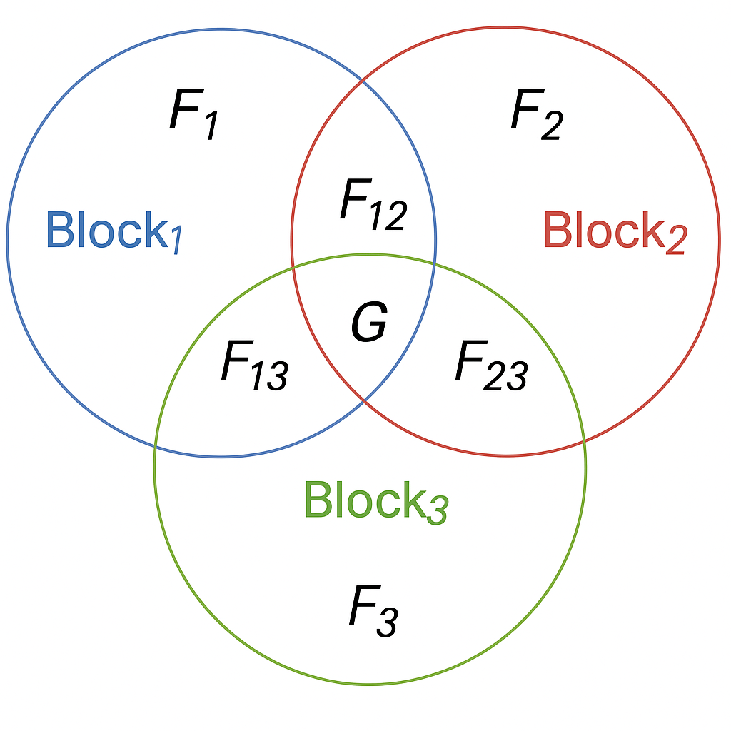
Figure 1: Factor structure formed by three different overlapping blocks of data.

2.2.3 Sequential least squares estimation

Estimation of the ML-DFM is based on the sequential approach proposed by Breitung2016 in which the main goal is to minimize the following residual sums of squares (RSS) function:

$$S(\hat{F_{t}},\hat{P})=\sum_{t=1}^{T}\left(X_{t}-\hat{P}\hat{F_{t}}\right)^{\prime}\left(X_{t}-\hat{P}\hat{F_{t}}\right),$$ (4)

by a sequence of LS regressions. The algorithm can be executed for the general case of $K$ blocks with overlapping factors as follows:

1. Obtain the initial values of the factors as follows:

   1. Employ canonical correlation analysis (CCA) on $X_{k,t}$ to obtain initial estimates of the global factor, $\hat{G}^{(0)}=\left(\hat{G}^{(0)}_{1},\hat{G}^{(0)}_{2},\dots,\hat{G}^{(0)}_{T}\right)^{\prime}$.

   2. Filter out the global component by regressing $X_{k,t}$ on $\hat{G}^{(0)}$, and get the corresponding residuals, $X^{*(0)}_{k,t}$, from each of the $K$ separate regressions.

   3. Employ CCA on $X^{*(0)}_{k,t}$ to obtain the following lower-level factors, selecting the corresponding blocks.

   4. Regress $X^{*(0)}_{k,t}$ on the respective lower-level factors involved and get the residuals.

   5. Steps c) and d) are executed sequentially until the initial estimates of the pairwise block factors are obtained. Denote by $X^{**(0)}_{k,it}$ the residuals after filtering the pairwise factors of each block $k$.

   6. Run PC on $X^{**(0)}_{k,t}$ to get the specific-block factors $\hat{F}^{(0)}=\left(\hat{F}^{(0)}_{1,t},\hat{F}^{(0)}_{2,t},\dots,\hat{F}^{(0)}_{k,t}\right)^{\prime}$.

   7. The initial matrix of loadings, $\hat{P}^{(0)}$, is estimated through time-series regressions of $X_{k,t}$ on the global factors, $X^{*}_{k,t}$ on the semi-pervasive factors, and $X^{**}_{k,t}$ on the non-pervasive factors.

2. Updated estimates for the unobservable factors $\hat{F}^{(1)}$ are obtained by LS regression of $X_{k,t}$ on $\hat{P}^{(0)}$ as follows $\hat{F}^{(1)}=\left(\hat{P}^{(0)^{\prime}}\hat{P}^{(0)}\right)^{-1}\hat{P}^{(0)^{\prime}}X_{k,t}$.

3. The updated factors $\hat{F}^{(1)}$ are used to obtain the associated loadings matrix, $\hat{P}^{(1)}$, as in Step 1.

4. Steps 2 and 3 are repeated until the RSS converges to a minimum, from which $\hat{F}^{*}$ and $\hat{P}^{*}$ are obtained.

As can be seen, the algorithm does not impose any normalization step. Henceforth, even though the vector of common components $P^{*}F_{t}^{*}$ is consistently estimated and just-identified, the factor and loading matrices themselves are not separately identified; they can only be estimated consistently up to a rotation of the factor space.

Breitung2016 adapt the standard normalization step in PC analysis to separately identify $P^{*}$ and $F_{t}^{*}$. The first step requires orthogonalizing the different levels of estimated factors (pervasive, pairwise, and block-specific) with respect to one another. A practical implementation consists of recursively regressing each factor on the previously ordered ones and using the residuals as updated, orthogonalized estimates. For instance, block-specific factors can be regressed on pairwise factors, and the resulting residuals can then be regressed on pervasive factors. Since each regression corresponds to a projection operation, this sequential procedure is equivalent to applying the Gram-Schmidt orthogonalization process to the vector of estimated factors $F_{t}^{*}$, following a predetermined ordering. Finally, the normalized pervasive factors are obtained as the top $\textbf{r}_{G}$ principal components of the estimated common components. These are derived from the nonzero eigenvalues and the corresponding eigenvectors of the matrix

$$\widehat{M}\left(\frac{1}{T}\sum_{t=1}^{T}\widehat{G}_{t}\widehat{G}_{t}^{\prime}\right)\widehat{M}^{\prime}.$$

The same normalization procedure can be applied to the semipervasive and block-specific factors, using the sample covariance matrices of their respective common components.

As explained earlier, the algorithm requires a suitable initialization of $P^{*}$ and $F_{t}^{*}$. The FARS package provides two initialization options: CCA and, alternatively, PC. While both approaches yield approximately the same estimated common components $P^{*}F_{t}^{*}$, CCA typically leads to faster convergence, requiring fewer iterations to minimize the RSS. However, when the factor structure is highly complex, initializing with PC tends to be computationally more efficient. See also Breitung2016 for the small sample properties of the sequential LS estimator with CCA and PC for the two-level DFM.

2.3 Probability distribution of factors

Constructing probabilistic scenarios requires knowledge of the joint distribution of the unobservable factors. The asymptotic distribution of such factors obtained from the DFM by PCA in (1) is derived by Bai2003InferentialDimensions. He shows that if $\frac{F^{\prime}F}{T}=I_{r}$ and $\frac{\sqrt{N}}{T}\rightarrow 0$ when $N,T\rightarrow\infty$, the asymptotic distribution of $\widehat{F}_{t}$, at each moment, $t$, is given by

$$\sqrt{N}\left(\widehat{F}_{t}-F_{t}\right)\overset{d}{\rightarrow}N\left(0,\Sigma_{P}^{-1}\Gamma_{t}\Sigma_{P}^{-1}\right),$$ (5)

where $\Sigma_{P}=\lim_{N\rightarrow\infty}\frac{P^{\prime}P}{N}$ and $\Gamma_{t}=\lim_{N\rightarrow\infty}\sum_{i=1}^{N}\sum_{j=1}^{N}p_{i}p_{j}^{\prime}E(\varepsilon_{it}\varepsilon_{jt})$ with $p_{i}$ and $\varepsilon_{it}$ being defined as in the DFM in (1). The finite sample approximation of the asymptotic covariance matrix of $\widehat{F}_{t}$ can be estimated as follows:

$$MSE_{t}=\left(\frac{\hat{P}^{\prime}\hat{P}}{N}\right)^{-1}\frac{\hat{\Gamma}_{t}}{N}\left(\frac{\hat{P}^{\prime}\hat{P}}{N}\right)^{-1},$$ (6)

where $\hat{\Gamma}_{t}$ is a consistent estimator for $\Gamma_{t}$. Under the assumption of cross-sectionally uncorrelated idiosyncratic components, BaiNg2006 propose the following estimator:

$$\widehat{\Gamma}^{BN}_{t}=\frac{1}{N}\sum_{i=1}^{N}\hat{p}_{i}\hat{p}_{i}^{{}^{\prime}}\hat{\varepsilon}_{it}^{2},$$ (7)

where $\hat{\varepsilon}_{it}=x_{it}-\hat{p}_{i}^{{}^{\prime}}\hat{F_{t}}$ are the residuals from the DFM model.

In many empirical settings, assuming that the idiosyncratic covariance matrix $\Sigma_{\epsilon}$ is diagonal imposes a stringent restriction that may not hold in practice. Therefore, alternatively, we can relax this assumption and allow the idiosyncratic components to be weakly cross-sectionally correlated. Under those circumstances, $\Gamma_{t}$ can be consistently estimated as proposed by Fresoli2024 by using adaptive thresholding of the sample covariances of the idiosyncratic residuals, $\hat{\sigma}_{ij}$, as follows:

$$\widetilde{\Gamma}^{FPR}=\frac{1}{N}\sum_{i=1}^{N}\sum_{j=1}^{N}\hat{p}_{i}\hat{p}^{\prime}_{j}\frac{1}{T}\sum_{t=1}^{T}\hat{\varepsilon}_{it}\hat{\varepsilon}_{jt}I\left(\mid\hat{\sigma}_{ij}\mid\geq c_{ij}\right),$$ (8)

where $I(\dot{)}$ is the indicator function that takes value one when the argument is true and zero otherwise, and $c_{ij}=\delta\omega_{NT}\left[\widehat{Var}\left[\hat{\varepsilon}_{it}\hat{\varepsilon}_{jt}\right]\right]^{1/2}$, with $\widehat{Var}\left[\hat{\varepsilon}_{it}\hat{\varepsilon}_{jt}\right]=\frac{1}{T}\sum_{t=1}^{T}\left[\hat{\varepsilon}_{it}\hat{\varepsilon}_{jt}-\hat{\sigma}_{ij}\right]^{2}$, $\omega_{NT}=\frac{1}{\sqrt{N}}+\sqrt{\frac{\text{log}(N)}{T}}$, and $\delta$ chosen as proposed by qiu2019.

It is important to note that the estimator of $\Gamma_{t}$ in (8) requires stationarity and, consequently, is constant over time. However, the estimator in (7), which does not require stationarity, may not be adequate for moderate levels of cross-sectional idiosyncratic correlation.

The asymptotic covariance matrix estimated as in (6) does not account for the uncertainty arising from the estimation of the loading matrix, regardless of whether $\Gamma_{t}$ is obtained from (7) or (8). In this light, Maldonado2021 propose a correction of the asymptotic MSE based on subsampling in the cross-sectional space subsets of series of size $N^{*}<N$, with each series in the subsample containing all temporal observations. For each subsample, the loadings and factors are estimated by PC, obtaining $\hat{F}_{t}^{*(s)}$ and $\hat{P}^{*(s)}$, for $s=1,...,S$. The corrected finite sample approximation of the asymptotic MSE of $\hat{F}_{t}$ can be estimated as follows:

$$MSE^{\ast}_{t}=\frac{1}{N}\left(\frac{\hat{P}^{\prime}\hat{P}}{N}\right)^{-1}\hat{\Gamma}_{t}\left(\frac{\hat{P}^{\prime}\hat{P}}{N}\right)^{-1}+\frac{N^{*}}{NS}\sum_{s=1}^{S}\left(\left(\hat{F}_{t}^{\ast(s)}-\hat{F}_{t}\right)\left(\hat{F}_{t}^{\ast(s)}-\hat{F}_{t}\right)^{\prime}\right),$$ (9)

where $\hat{\Gamma}_{t}$ can be estimated as in (7) or in (8).

Based on the asymptotic normality result in (5), Maldonado2021 construct confidence ellipsoids for the estimated factors with coverage probability $100\times\alpha\%$ as follows:

$$g(F_{t},\alpha)=\{F_{t}\in{\rm I\!R}^{r}|(F_{t}-\hat{F_{t}})MSE_{t}^{*-1}(F_{t}-\hat{F_{t}})\leq\chi^{2}_{r(\alpha)}\},$$ (10)

where $\chi^{2}_{r(\alpha)}$ is the $\alpha$-quantile of the $\chi^{2}$ distribution with $r$ degrees of freedom, with $r$ being the number of factors. Each point on the surface of the ellipsoid represents a possible joint realization of all factors in the DFM. These boundary points correspond to extreme, yet plausible, stress conditions.

2.4 Density Forecasts Under Stressed and Non-Stressed Conditions

Estimated factors can be used to summarize the information contained in a large set of predictors $X_{t}$, which are used to estimate the temporal evolution of the conditional density of a target variable. In this subsection, we describe how these densities can be obtained under both stressed and non-stressed conditions for the underlying factors.

Let $y_{t}$ be the observation at time $t$ of the target variable. We start by obtaining $h$-step-ahead forecasts of the $\tau^{*}$-quantile of the conditional distribution of $y_{t}$ by estimating the following FA-QR:

$$q_{\tau^{*}}(y_{t+h}\mid y_{t},F_{t})=\mu(\tau^{*},h)+\phi(\tau^{*},h)y_{t}+\sum_{k=1}^{r}\beta_{k}(\tau^{*},h)F_{kt},$$ (11)

where $\mu(\tau^{*},h)$, $\phi(\tau^{*},h)$, and $\beta_{k}(\tau^{*},h)$ for $k=1,\ldots,r$, are parameters, and ${F}_{t}$ is the $r\times 1$ vector of the underlying unobserved factors at time $t$. In practice, the underlying factors in (11) are replaced by their estimations, $\hat{F}_{t}$, obtained as described above.

The parameters of the FA-QR model in (11) are estimated using the algorithm by KoenkerOrey1987, which implements the quantile regression method originally developed by Koenker1978. When the error terms are assumed to be independently distributed according to a Laplace distribution, the estimator coincides with the Maximum Likelihood (ML) estimator; see Ando2011QuantileCriterion. BaiandNg2008 establishes its asymptotic normality.

The FA-QR provides estimates of the quantile function of the target variable, $\widehat{q}_{\tau^{*}}(y_{t+h}|y_{t},F_{t})$, for several values of $\tau^{*}$. In practice, however, it is challenging to map these estimates into a probability distribution function due to approximation errors and estimation noise. Consequently, as in Adrian2019, we use the skew-t distribution proposed by Azzalini2003 to smooth the quantile function and estimate the conditional density of $y_{t}$. The skew-t density depends on four parameters as follows:

$$f(y;\mu,\sigma,\alpha,v)=\frac{2}{\sigma}st\left(\frac{y-\mu}{\sigma};v\right)sT\left(\alpha\frac{y-\mu}{\sigma}\sqrt{\frac{v+1}{v+\left(\frac{y-\mu}{\sigma}\right)^{2}}};v+1\right),$$ (12)

where $st(\cdot)$ and $sT(\cdot)$ denote the probability density function and the cumulative distribution function of the Student’s t distribution, respectively. The skew-t distribution is specified by its location $\mu$, scale $\sigma$, shape $\alpha$, and fatness $v$. At each time $t$, a skew-t distribution is fitted by choosing the parameters that minimize the squared differences between the quantile estimates and the skew-t implied quantiles, $q_{\tau^{*}}(y;\mu,\sigma,\alpha,v)$, as follows:

$$(\hat{\mu}_{t+h},\hat{\sigma}_{t+h},\hat{\alpha}_{t+h},\hat{v}_{t+h})=\underset{\mu,\sigma,\alpha,v}{\operatorname{argmin}}\sum_{t=1}^{T-h}(\widehat{q}_{\tau^{*}}(y_{t+h}\mid y_{t},F_{t})-q_{\tau^{*}}(y_{t};\mu,\sigma,\alpha,v))^{2}.$$ (13)

The methodology described above estimates the conditional density of $y_{t}$ under non-stressed conditions. To construct conditional densities based on stressed scenarios, Gonzlez-Rivera2019 and Gonzlez-Rivera2024 use the confidence ellipsoids defined in (10), and determine the value of the factors on the $\alpha\%$-contour (stress level of the underlying factors) that minimize (or maximize) a given quantile ($\tau$) of the conditional distribution of the target variable. For instance, consider that we are interested in deriving a stress scenario for $\tau=0.05$, with the factors stressed at their $\alpha\%$ level, FARS solves the following optimization problem at each moment:

$${\min_{F_{t}^{(S)}}}\;\hat{q}_{0.05}(y_{t+h}|y_{t},F_{t}^{(S)})$$ (14)

$$s.t.\quad g(F_{t}^{(S)},\alpha)=0,$$

where $g(F_{t}^{(S)},\alpha)=0$ is a predetermined $\alpha$-contour of the factors, that is, an ellipsoid that contains $F_{t}$ with probability $\alpha$.

The values of $F_{t}^{(S)}$ on the boundary of the ellipsoid $g(F_{t}^{(S)},\alpha)=0$ represent extreme events of the factors. After solving the optimization problem in (14), these optimized values are plugged into the estimated FA-QRs. The conditional density of $y_{t}$ under stress is then obtained by smoothing the corresponding quantiles as described in (13).

3 The FARS package

In this section, we provide a detailed overview of the FARS package functionalities and explain how users can implement the methodology described in Section 2 using the available functions.

3.1 ML-DFM in FARS

We begin by introducing the mldfm() function, which provides users with a flexible tool for extracting factors using either DFM or ML-DFM, with either non-overlapping or overlapping blocks. In the case of a simple DFM, the function requires two input arguments. The first is data, which contains the N variables from which the factors are extracted, structured as a $T\times N$ matrix. The second argument is global, which specifies the number of factors $r$ to be extracted from the data.

In the case of the ML-DFM without overlapping blocks, additional arguments must be provided to the mldfm function: i) the argument blocks defines the number of blocks $K$ that make up the data sample (the default is 1, corresponding to the DFM case); ii) block_ind requires a vector that indicates the indices of the end column for each block $k$. For example, if $K=3$ and $N=N_{1}+N_{2}+N_{3}$, the argument block_ind should contain $[N_{1},N_{1}+N_{2},N_{1}+N_{2}+N_{3}]$; iii) the argument local is a vector of integers, indicating the number of block-specific factors $r_{F_{k}}$ to be extracted from each block $k$; iv) global specifies the number of pervasive factors $r_{G}$; v) method defines the factor initialization strategy for the sequential LS estimation: 0 for the CCA (default) and 1 for PCA; vi) the arguments tol and max_iter define the tolerance level and the maximum number of iterations allowed for the RSS minimization process, with default values set to $10^{-6}$ and $1000$, respectively.

In the case of the ML-DFM with overlapping blocks, an additional middle_layer argument must be provided. middle_layer is a named list, where each name is a string specifying a group of overlapping blocks (e.g. $kj$ in the case of pairwise groups), and each value is the number of factors $r_{{kj}}$ to extract from that group. For example, if we want to extract one pairwise factor from blocks 1 and 3 ($r_{{13}}=1$), the list should be defined as list("1-3" = 1).

Regardless of the particular specification of the model, the mldfm() function returns an S3 object of class mldfm as output. The object is a list containing several attributes described in Table 1.

Attribute	Description
Factors	$T\times r$ matrix containing all the extracted factors.
Lambda	$N\times r$ matrix of factor loadings with necessary zero restrictions.
Residuals	$T\times N$ residual matrix from the model fit.
Method	The initialization strategy used (CCA or PCA).
Iterations	Number of iterations performed until convergence (0 in DFM).
Factors_list	A summary list indicating the number of factors extracted at each level.

Table 1: Attributes of the mldfm object. The $r$ factors in the Factors and Lambda matrices follow the hierarchical order (from global to local) described in Factors_list.

The mldfm object has typical S3 methods: print(), summary() and plot(). The first two functions offer a brief overview of the model estimation outcome, while plot() offers pre-configured visualization tools. The call of the plot function on a mldfm object generates distinct line charts for all estimated factors, each enriched with confidence interval bands that assume cross-sectionally independent and homoskedastic idiosyncratic components. Furthermore, an optional input argument dates can be provided. dates is a vector of dates to be displayed on the x-axis, replacing the default integer time index ranging from 1 to $T$. Moreover, using the plot() function, it is possible to visualize estimated loadings or residuals, specifying a which argument with values "loadings" or "residuals". With "loadings", a singular figure is generated, which contains a set of bar charts displaying the estimated loadings along with their corresponding pairwise confidence intervals. Differently, with "residuals", a figure depicting the correlation heatmap of the residuals is produced. In both cases, the user can provide a list of variable names using the optional var_names argument. This enables the replacement of the default indexes from VAR 1 to VAR N with the appropriate variable names.

3.2 Probability distribution of factors in FARS

A two-step procedure is implemented in FARS to obtain the asymptotic joint probability density of the factors with the subsampling correction.

The first step involves running a subsampling method to extract factors from subsets of $N^{*}$ variables, selected from the entire data sample. This is implemented using the mldfm_subsampling() function. The function iteratively generates n_samples subsamples of size sample_size and estimates factors using the ML-DFM approach through the mldfm() function. This approach offers two main advantages. First, the arguments of mldfm_subsampling() are the same as those of mldfm(), with the addition of two additional arguments to define the number and size of the subsamples. Second, the function returns a list of mldfm objects, enabling the user to apply standard methods such as summary(), print(), and plot() to each of the subsample results. In addition, an optional seed argument can be provided to ensure the reproducibility of the results.

The second step involves constructing confidence regions for the factors, as outlined in equation (10). This operation is performed by the create_scenario() function, which requires three main arguments. The first is model, which contains the result of the mldfm() function applied to the full dataset and serves as the center of the ellipsoid. The second is subsample, which takes the output of mldfm_subsampling(), a list of mldfm objects obtained from each subsample, and uses it to compute the MSE correction as defined in Equation (9). The third is alpha, which defines the coverage probability (i.e., the level of stress) for the ellipsoids. An optional argument, atcsr, can be set to TRUE to estimate the asymptotic MSE of the factors using $\widetilde{\Gamma}^{\text{FPR}}$ as defined in equation (8). Differently, the default setup (FALSE) uses $\hat{\Gamma}_{t}^{\text{BN}}$ as described in Equation (7). The output of create_scenario() is a list of $T$ matrices of size $z\times r$ representing the ellipsoid points in $r$ dimensions for each time observation $t$. The number of points $z$ depends on the number of dimensions $r$. In the case of only one factor ($r=1$), only a confidence interval is built based on the specified alpha level; for this reason, $z=2$ (i.e., the upper and the lower bounds). In the case of two dimensions ($r=2$), the 2-D ellipsoid is composed of $z=300$ points and is built using the ellipse package; see ellipse. Lastly, in the case of more than two dimensions ($r>2$), the $r$-D ellipsoid is generated through the hyperellipsoid() and hypercube_mesh() functions from the SyScSelection package (SyScSelection). In this case, the number of points composing the ellipsoid depends on the phi parameter of the hypercube_mesh() function, which defines the scalar fineness of the mesh. In FARS, phi is set to 8.

3.3 Conditional Density Under Stressed and Non-Stressed Conditions in FARS

In this section, we present the tools provided by FARS for obtaining conditional density forecasts in both the non-stressed and stressed scenarios.

The first step is to estimate the FA-QRs. This operation is performed through the compute_fars() function, which estimates the parameter of the FA-QR in Equation (11). In the non-stressed setup, the function requires only three arguments to work. First, dep_variable, which contains the dependent variable $y$. Second, factors, which includes the factors the user wants to add to the quantile regression model. Third, h, which defines the forecast horizon (the default is $h=1$). The function estimates the FA-QRs for a fixed set of quantiles: 0.05, 0.25, 0.50, 0.75, and 0.95, as these are later used for the skew-t density fit. Alternatively, the user can modify the extreme quantiles by setting an optional edge argument. For example, setting edge = 0.01 forces the edge quantiles to 0.01 and 0.99. The default value is 0.05. In the stressed scenario setup, additional arguments are required. The scenario argument takes the list of ellipsoids produced by the create_scenario() function. Moreover, the user must define QTAU and min, which correspond to the quantile that will be minimized or maximized, and the optimization strategy used to compute stressed factors over the ellipsoid points. The default value for min is TRUE, which means that the objective is to minimize a given quantile of the target variable $y$. Differently, if min value is FALSE, the objective is to maximize the quantile of $y$. The output of compute_fars() is an S3 object of type fars, which contains a set of attributes listed in Table 2.

Attribute	Description
Quantiles	$T\times 5$ matrix containing the estimated quantiles.
Coeff	$(r+2)\times 5$ matrix containing the estimated coeffcients.
StdError	$(r+2)\times 5$ matrix containing the estimated standard errors.
Pvalue	$(r+2)\times 5$ matrix containing the estimated standard P-values.
Levels	The list of estimated quantiles.
QTAU*	The quantile selected for the min/max procedure.
Stressed_Factors*	$T\times r$ matrix containing the stressed factors.
Stressed_Quantiles*	$T\times 5$ matrix containing the estimated stressed quantiles.

Table 2: Attributes of the fars object. Attributes marked with * are included only if the user provides the necessary argument for the stressed scenario case.

Like the mldfm object, the fars object has standard S3 methods. The print() function provides a brief overview of the FA-QRs. The summary() function returns a detailed summary of quantile regression, including estimated coefficients, standard errors, and p-values for each quantile. Lastly, the plot() function generates two line charts: one composed of non-stressed quantiles and the second of stressed scenario quantiles. The function can display customized dates on the x-axis by setting the corresponding optional argument dates.

The second step to obtaining a density forecast is to estimate the conditional density of the target variable $y$ by fitting a skewed-t distribution. This operation is performed via the compute_density() function, which requires a quantiles argument, containing the quantiles estimated by the compute_fars() function. Depending on the quantiles provided, Quantiles or Stressed_Quantiles, the density function returns the non-stressed or the stressed conditional density, respectively. Additional arguments can be provided to compute_density(), including est_points, which set the number of estimation points (default is 512), random_samples, which define the number of random samples to be drawn from the estimated distribution (default is 5000) and support, which select the lower and upper bounds of the random variable support (default is c(-10,10)). For each period $t$, compute_density() initializes the skewed-t distribution by setting three parameters (location, scale, and shape) using the quantile values provided as input. The function implements two optimization procedures to fit the skew-t distribution. The default is a linear optimization using optim() from stats, which implements the L-BFGS-B method. The second is a non-linear optimization method that can be selected by setting the argument nl = TRUE. The non-linear method is from the nloptr package and is based on NLOPT_LN_SBPLX (NLopt). In both cases, the theoretical quantiles and the probability distribution function (pdf) of the fitted skewed-t distribution are computed using qst() and dst() from sn (snpkg), respectively. Finally, a seed argument can be provided to ensure the reproducibility of the results. The compute_density() function returns a fars_density object which provides the attributes listed in Table 3.

Attribute	Description
density	The estimated densities at time $t$.
distribution	The random draws from the fitted skew-t distribution at each $t$.
optimization	The optimization method implemented: linear or non-linear.
x_vals	The sequence of evaluation points used to compute the density.

Table 3: Attributes of the fars_density object. Both density and distribution are provided in matrix form with one row for each time $t$.

The fars_density object is equipped with standard S3 methods. The print() function provides a brief overview of the estimated density. The summary() function returns the mean, median, and standard deviation of the distribution at time $t$. Finally, the plot() function generates a 3D plot of the density, with evaluation points (x_vals) on the x-axis, time indices on the y-axis, and density values on the z-axis. The function can also display custom dates on the y-axis by setting the optional argument time_index.

The final step in obtaining a conditional density forecast is to extract the conditional quantile from the estimated skew-t distribution. This can be performed using the function quantile_risk(). This function requires two parameters: an object of class fars_density and the quantile that must be extracted QTAU. The quantile extraction is implemented via quantile() from stats. Depending on the fars_density object provided, either a non-stressed or a stressed density, the quantile_risk() extracts a non-stressed quantile or a stressed quantile of the target variable (e.g., in the case of GDP growth with QTAU = 0.05 ($T=59$), it extracts Growth-at-Risk or Growth-in-Stress).

Figure 2 shows a recap of the FARS package workflow for both the non-stressed and the stressed scenarios.

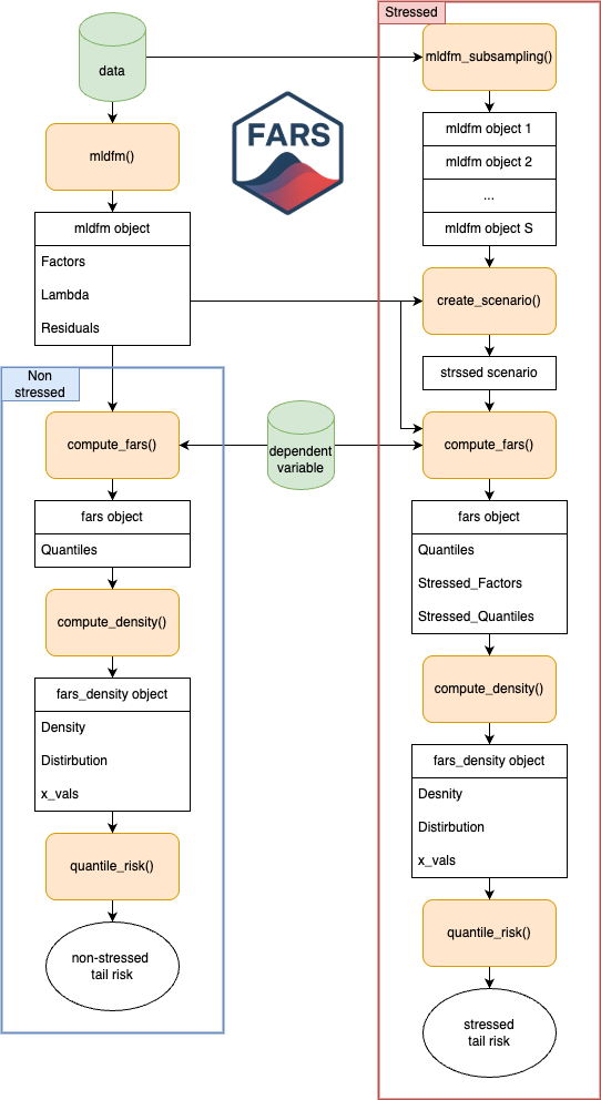
Figure 2: FARS package workflow for both non-stressed and stressed scenarios.

4 An application to conditional density of growth in the US economy

In this section, we illustrate the functionalities of the FARS package by building scenarios for US growth as in Gonzlez-Rivera2024. In this exercise, we implement an ML-DFM using a data sample composed of three blocks. The first block contains $N_{1}=63$ global macroeconomic variables (GDP growth for 63 countries), the second block contains $N_{2}=248$ domestic macroeconomic variables, and the third block contains $N_{3}=208$ global financial variables, observed quarterly from 2005Q3 to 2020Q1. The dependent variable is the annualized quarterly GDP growth for the US. Data are retrieved from the replication files of Gonzlez-Rivera2024.

The first step is to install and load the package. FARS is available to the public on CRAN under the GPL-3 license and can be downloaded as follows:

R> install.packages("FARS")

The development version is available on GitHub at https://github.com/GPEBellocca/FARS. This can be downloaded using the devtools package with the following command:

R> devtools::install_github("GPEBellocca/FARS")

After installing the package from CRAN or GitHub, the package should be loaded as follows:

R> library(FARS)

The dataset, composed of $N=N_{1}+N_{2}+N_{3}=519$ variables, is stored in the data matrix, while the US GDP growth is stored in dep_variable. To estimate an ML-DFM through mldfm(), we first need to decide how many factors to extract from each block. Following Gonzlez-Rivera2024, we extract a global factor from the three blocks, a pairwise factor from the global macroeconomic and global financial blocks (1 and 3), and one local factor from each of the three blocks. This operation is performed as follows:

R> mldfm_result <- mldfm(data, + blocks = 3, + block_ind = c(63,311,519), + global = 1, + local = c(1,1,1), + middle_layer = list("1-3" = 1))

Since we are not providing any method, tol, and max_iter, the default values are enforced. The mldfm object returned is stored in the mldfm_result variable. After completion, the function summary() can be used to display an overview of the estimated ML-DFM, including the number of factors extracted at each level of the hierarchical structure used in the Sequential LS estimation.

R> summary(mldfm_result) Summary of Multilevel Dynamic Factor Model (MLDFM) =================================================== Number of periods: 59 Number of factors: 5 Number of nodes: 5 Initialization method: CCA Number of iterations to converge: 47

Number of factors per node: - 1-2-3 : 1 factor(s) - 1-3 : 1 factor(s) - 1 : 1 factor(s) - 2 : 1 factor(s) - 3 : 1 factor(s)

Residual sum of squares (RSS): 15215.6724 Average RSS per period: 257.8928

Additionally, using plot(), it is possible to obtain a graphical representation of the estimated factors, loadings, and residuals. For illustration, we extract two factors from the global macroeconomic block of variables as follows:

R> mldfm_result_gm <- mldfm(data = data[, 1:63], blocks = 1, global = 2)

Then, we call the plot function three times to plot the estimated factors, loadings, and residuals, in sequence. For a more precise result, we provide the plot function with appropriate arrays composed of dates and variable names using the optional arguments.

R> plot(mldfm_result_gm, dates = dates) R> plot(mldfm_result_gm, which = "loadings", var_names = var_names) R> plot(mldfm_result_gm, which = "residuals", var_names = var_names)

The results are plotted in Figures 3, 4 and 5, respectively. After estimating the ML-DFM we can now build the non-stressed and stressed scenarios following the steps depicted in Figure 2.

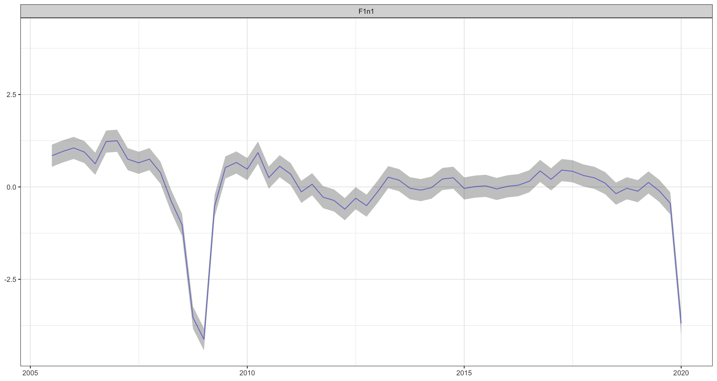
(a) Factor 1

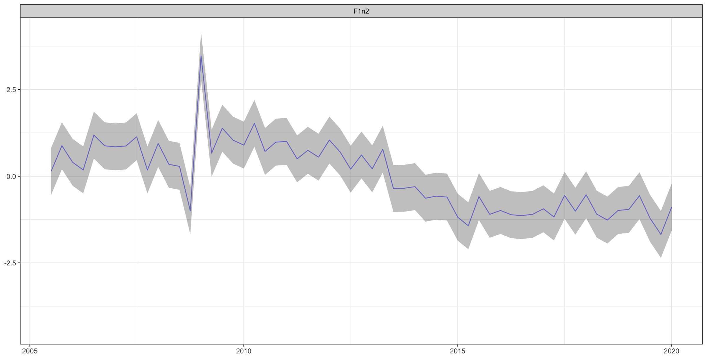
(b) Factor 2

Figure 3: Line chart of extracted factors.

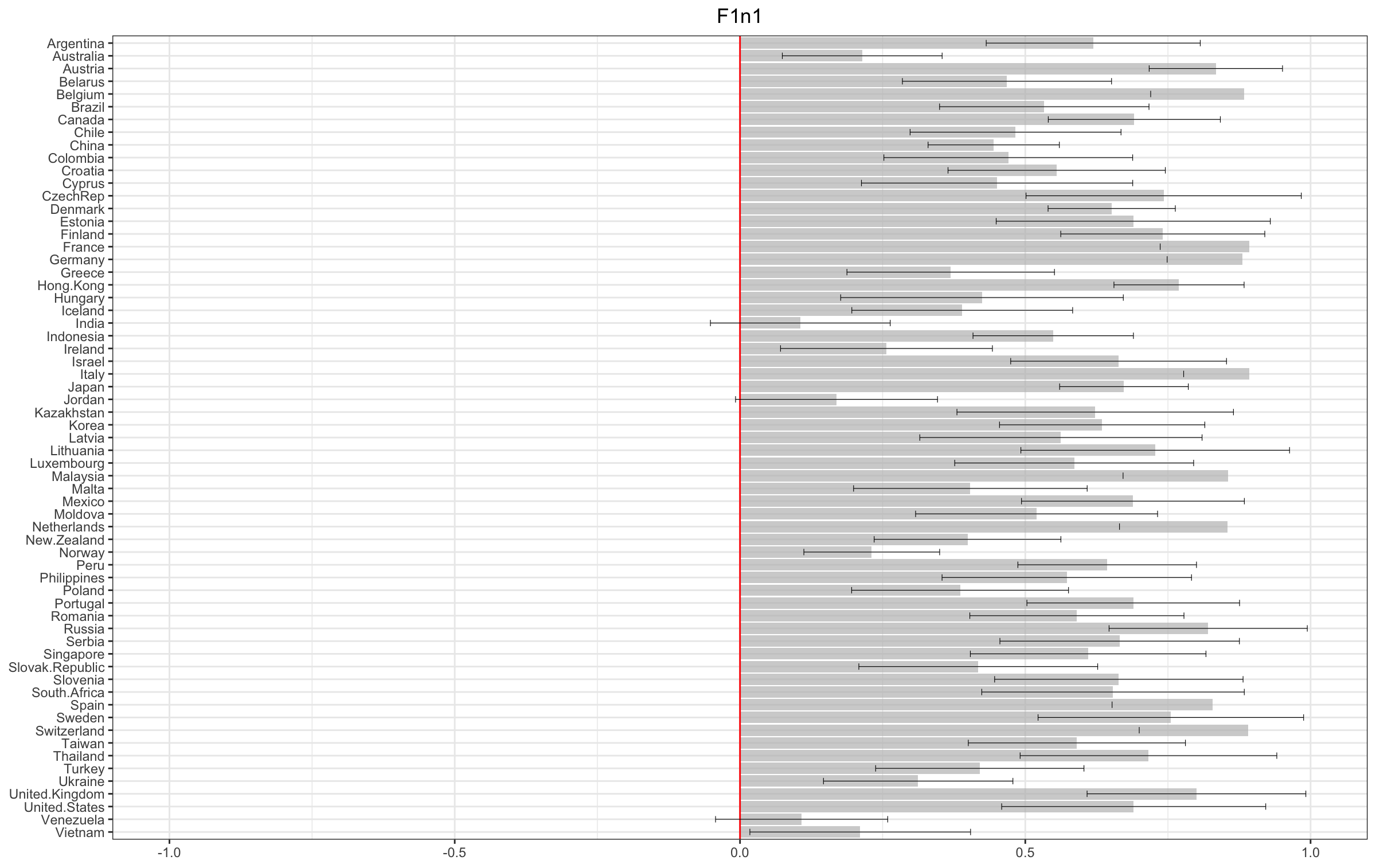
(a) Loadings for factor 1

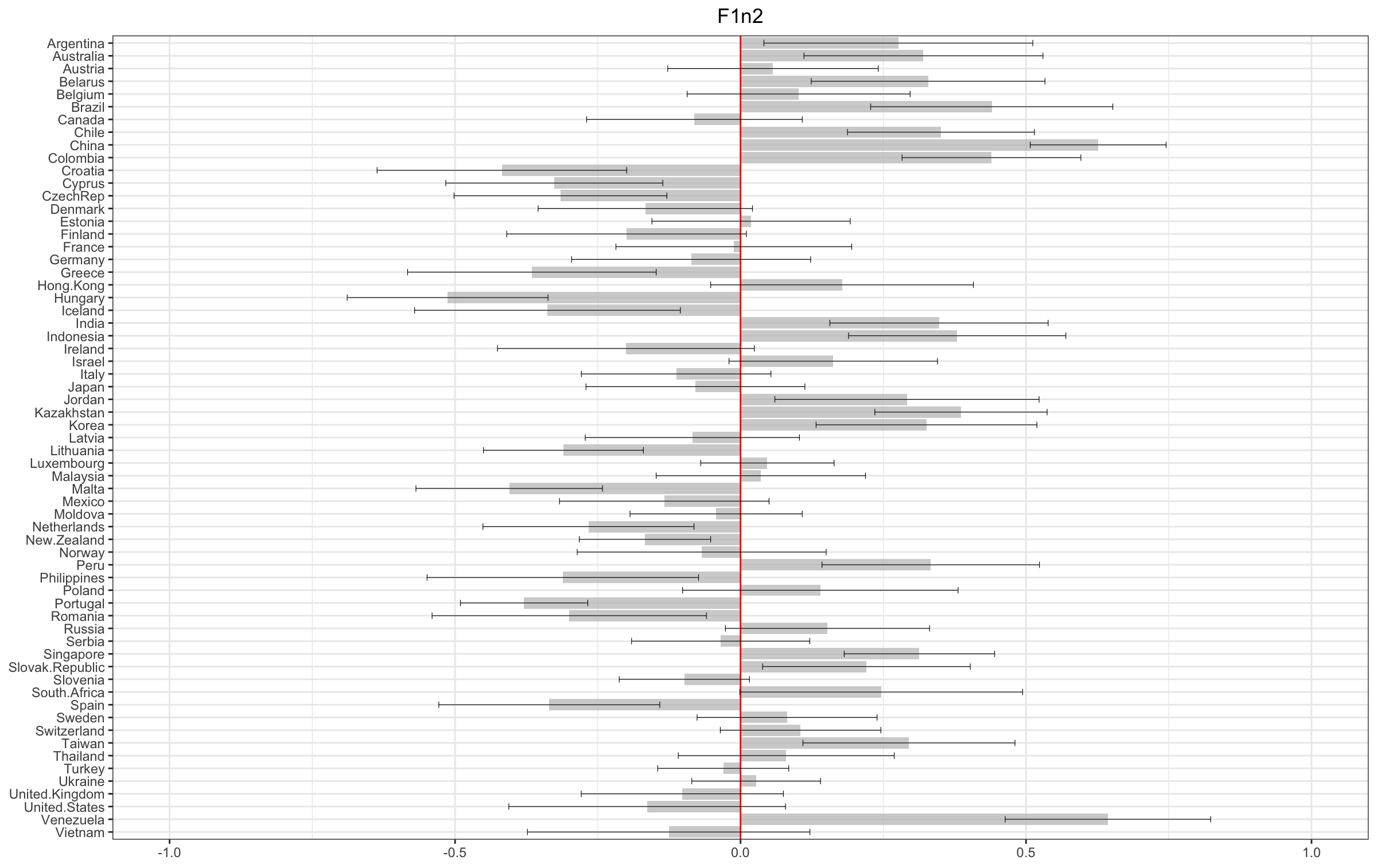
(b) Loadings for factor 2

Figure 4: Bar chart of factor loadings.

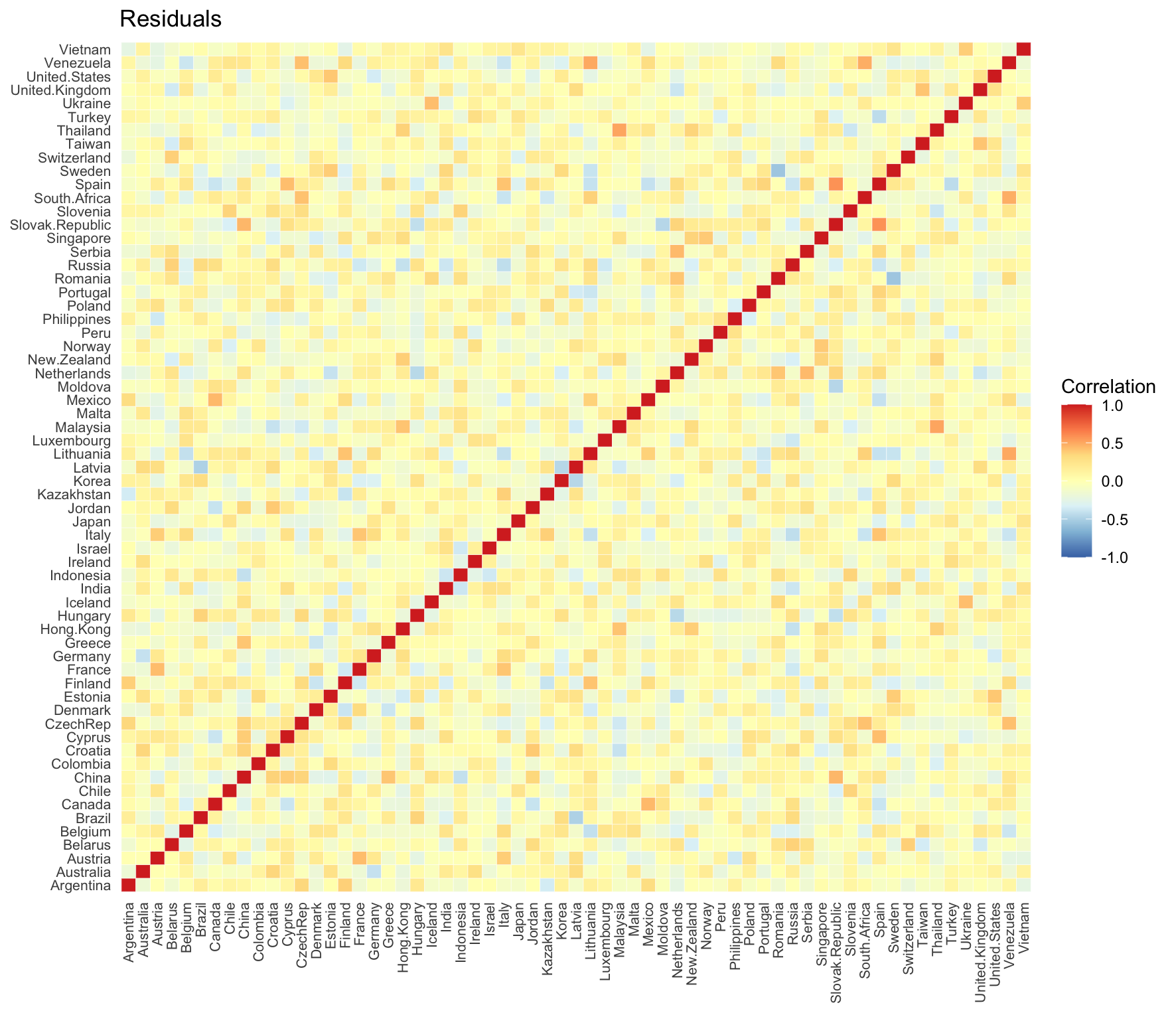
Figure 5: Residual correlation heatmap.

4.1 Non-stressed scenario

The first step to build the unstressed scenario is to estimate the FA-QRs as follow:

R> fars_result <- compute_fars(dep_variable, mldfm_result$Factors,h=1)\CodeOutput RunningFactor-AugmentedQuantileRegressions(FA-QRs)...Completed\par Afterthis,wecanplotthequantilesforthenon-stressedscenario(seeFigure\ref{fig:quantiles},panela)andprintarecapoftheFA-QRs.\par\CodeChunk\CodeInput R>plot(fars_{r}esult,dates=dates)R>print(fars_{r}esult)\CodeOutput Factor-AugmentedQuantileRegressions(FARS)===========================================Forecastedquantiles:-Numberofperiods:59-Quantilelevels:0.050.250.500.750.95\par Stressedquantiles:NO\par\begin{figure}[h]\centering\begin{subfigure}{433.62pt}\centering\includegraphics[width=433.62pt]{Figures/quantiles.png}\@@toccaption{{\lx@tag[ ]{{(a)}}{Non-stressedscenario}}}\@@caption{{\lx@tag[ ]{{\small(a)}}{\small Non-stressedscenario}}}\@add@centering\end{subfigure}\vskip 12.0pt\begin{subfigure}{433.62pt}\centering\includegraphics[width=433.62pt]{Figures/strssed_quantiles.png}\@@toccaption{{\lx@tag[ ]{{(b)}}{Stressedscenario}}}\@@caption{{\lx@tag[ ]{{\small(b)}}{\small Stressedscenario}}}\@add@centering\end{subfigure}\@@toccaption{{\lx@tag[ ]{{6}}{Non-stressedandstressedscenarioquantiles.}}}\@@caption{{\lx@tag[: ]{{\small Figure 6}}{\small Non-stressedandstressedscenarioquantiles.}}}\@add@centering\end{figure}\par\par Theresultsstoredin\code{fars_{r}esult}arethenusedtofitaskew-tdistribution,generatingthedensityforthenon-stressedscenariobasedon\code{fars_{r}esult\$Quantiles}.ThisisdonebyapplyingthedefaultlinearoptimizationmethodandprovidinganappropriatesupportforourGDPgrowthcase.\par\CodeChunk\CodeInput R>ns_{d}ensity<-compute_{d}ensity(fars_{r}esult$Quantiles,support=c(-30,10),seed=42)\CodeOutput Estimatingskew-tdensitiesfromforecastedquantiles...Completed\par Thegenerated\code{fars_{d}ensity}objectcanbeusedtoplotthenon-stresseddensity(seeFigure\ref{fig:densities},panela)andvisualizeanoverviewofthedensityestimation.\par\CodeChunk\CodeInput R>plot(ns_{d}ensity,time_{i}ndex=dates)R>print(ns_{d}ensity)\CodeOutput FARSDensity====================Timeobservations:59Estimationpoints:512Randomsamples:5000Supportrange:[-30,10]Optimization:Linear\par\begin{figure}[h]\centering\begin{subfigure}{433.62pt}\centering\includegraphics[width=433.62pt]{Figures/normal_density.png}\@@toccaption{{\lx@tag[ ]{{(a)}}{Non-stresseddensity}}}\@@caption{{\lx@tag[ ]{{\small(a)}}{\small Non-stresseddensity}}}\@add@centering\end{subfigure}\vskip 12.0pt\begin{subfigure}{433.62pt}\centering\includegraphics[width=433.62pt]{Figures/stressed_density.png}\@@toccaption{{\lx@tag[ ]{{(b)}}{Stresseddensity}}}\@@caption{{\lx@tag[ ]{{\small(b)}}{\small Stresseddensity}}}\@add@centering\end{subfigure}\@@toccaption{{\lx@tag[ ]{{7}}{Non-stressedandstresseddensities.}}}\@@caption{{\lx@tag[: ]{{\small Figure 7}}{\small Non-stressedandstresseddensities.}}}\@add@centering\end{figure}\par Finally,weestimatetheGaRatQTAU=0.01applyingthe\code{quantile_{r}isk()}functiontothenon-stresseddensity.\par\CodeChunk\CodeInput R>GaR<-quantile_{r}isk(ns_{d}ensity,QTAU=0.01)\par$

4.2 Stressed scenario

As explained in Section 3, the computation of the stressed scenario can be performed in two steps. First, we need to obtain the asymptotic distribution of the factors. For this goal, we implement the subsampling procedure using the appropriate function. In our case, we generate 100 samples by extracting $94\%$ of the variables from each block.

R> mldfm_ss_result <- mldfm_subsampling(data, + blocks = 3, + block_ind = c(63,311,519), + global = 1, + local = c(1,1,1), + middle_layer = list("1-3" = 1), + n_samples = 100, + sample_size = 0.94, + seed = 42) Generating 100 subsamples…

Subsampling completed. Number of subsamples generated: 100

Each of the 100 elements stored in mldfm_ss_result list can be manipulated as a distinct mldfm object. For example, we can visualize the summary of the ML-DFM estimated for sample number 10.

R> summary(mldfm_ss_result[[10]]) Summary of Multilevel Dynamic Factor Model (MLDFM) =================================================== Number of periods: 59 Number of factors: 5 Number of nodes: 5 Initialization method: CCA Number of iterations to converge: 53

Number of factors per node: - 1-2-3 : 1 factor(s) - 1-3 : 1 factor(s) - 1 : 1 factor(s) - 2 : 1 factor(s) - 3 : 1 factor(s)

Residual sum of squares (RSS): 14212.7382 Average RSS per period: 240.8939

The second step to generate the stressed scenario is calling the create_scenario() function. For this exercise, we consider the highest stress level of alpha = 0.99 and default $\hat{\Gamma}_{t}^{\text{BN}}$.

R> scenario <- create_scenario(model = mldfm