Optimal Calibration of Qubit Detuning and Crosstalk

Abstract

Characterizing and calibrating physical qubits is essential for maintaining the performance of quantum processors. A key challenge in this process is the presence of crosstalk that complicates the estimation of individual qubit detunings. In this work, we derive optimal strategies for estimating detuning and crosstalk parameters by optimizing Ramsey interference experiments using Fisher information and the Cramér–Rao bound. We compare several calibration protocols, including measurements of a single quadrature at multiple times and of two quadratures at a single time, for a fixed number of total measurements. Our results predict that the latter approach yields the highest precision and robustness in both cases of isolated and coupled qubits. We validate experimentally our approach using a single NV center as well as superconducting transmons. Our approach enables accurate parameter extraction with significantly fewer measurements, resulting in up to a 50% reduction in calibration time while maintaining estimation accuracy.

The biggest challenge for a quantum bit is standing still. Unlike classical bits, where friction can be used to maintain the same state over time, quantum bits (qubits) are always on the move. The most common motion of an idle qubit is a random rotation around the $Z$ axis, corresponding to a progressive randomization of the phase difference between the $|0\rangle$ and $|1\rangle$ states. To avoid this uncontrolled jitteriness, quantum computing providers need to frequently perform time-consuming calibrations on an hourly basis IBM_calibration ; private . This process delivers up-to-date values of the qubits’ rotation frequencies, or detunings, that are then used to tune the control fields used to generate quantum gates, see Refs. siddiqi2021engineering ; chatterjee2021semiconductor ; kjaergaard2020superconducting for an introduction.

The presence of unavoidable couplings between the qubits complicates the process of calibrating a quantum computer. In particular, superconducting quantum computers are characterized by a static “crosstalk” between neighboring qubits, which changes the detuning of one qubit depending on the state of the other qubits mundada2019suppression ; ni2022scalable ; xie2022suppressing ; heng2024estimatingeffectcrosstalkerror ; fors2024comprehensiveexplanationzzcoupling ; sarovar2020detecting . Due to these terms, the calibration process cannot be performed simultaneously on all the qubits. The goal of this work is to determine the optimal strategy for calibrating single-qubit and multi-qubit systems. We will demonstrate that by carefully selecting measurement times and quadratures, it is possible to save up to 50% of the time while maintaining fixed calibration precision.

To introduce our optimal strategy, we first consider the case of a single qubit, whose detuning $\omega$ is unknown. To mimic realistic conditions, we assume that the qubit undergoes a dephasing process. The dynamics of the qubit are then described by

$$H=\frac{\omega}{2}(1-Z)+h(t)(1-Z).$$ (1)

Here, $Z$ is a Pauli matrix with eigenvalues $+1$ and $-1$, respectively for the $|0\rangle$ and $|1\rangle$ states, and $h(t)$ is a Gaussian random process with $\langle h(t)\rangle=0$ and two-point correlation function $\langle h(t)h(t^{\prime})\rangle=F(t-t^{\prime})$ breuer2002theory ; benedetti2014effective ; Shirizly_2024 .

The common procedure to calibrate the qubit consists of a series of Ramsey interference experiment, where (i) an initial $\pi/2$ pulse prepares the qubit in the superposition state, $|+\rangle=(|0\rangle+|1\rangle)/\sqrt{2}$; (ii) the qubit is let evolve freely for time $t$; and (iii) the Pauli operator $X$ is measured by applying a second $\pi/2$ pulse and measuring the qubit in the computational basis. The experiment is repeated for varying $t$ and the average result is stored as $\langle X(t)\rangle_{\rm exp}$. This quantity is then compared to the theoretical result obtained by evolving the initial state with Eq. (1), $|\psi\rangle=\left[|0\rangle+\exp(-i\omega t-i\int_{0}^{t}dt^{\prime}~h(t^{\prime}))|1\rangle\right]/\sqrt{2}$ and averaging over $h(t)$, leading to $\langle X(t)\rangle_{\rm theory}=\cos(\omega t)\exp\left(-\tfrac{1}{2}\int_{0}^{t}dt^{\prime}\int_{0}^{t}dt^{\prime\prime}F(t^{\prime}-t^{\prime\prime})\right)$. If the noise correlations have short memory, one can approximate $F(t-t^{\prime})=\gamma\delta(t-t^{\prime})$, where $\gamma$ is the dephasing rate and $\delta(t-t^{\prime})$ is the Kronecker delta. In this case, often referred to as the Markovian limit, one obtains a closed expression that depends on $\omega$ and $\gamma$ only

$$\langle X(t)\rangle_{\rm theory}=\cos(\omega t)e^{-\gamma t}$$ (2)

These two parameters are then estimated by minimizing the difference between $\langle X(t)\rangle_{\rm exp}$ and $\langle X(t)\rangle_{\rm theory}$ qiskit_calibration . In the case of a noise bath with a correlation time $\tau_{\rm bath}$ comparable to $1/\gamma$, it is possible to derive an analytic expression that depends on both $\tau_{\rm bath}$ and $\gamma$ curtis2025non and can be easily incorporated in the present approach.

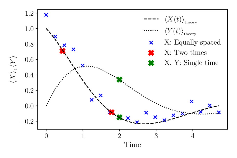
Figure 1: Three strategies to calibrate the frequency $\omega$ and dephasing rate $\gamma$ of a single qubit, respectively denoted by blue, red, and green crosses, see text for details. The blue strategy is noisier because it uses more measurement times with fewer shots in each of them.

In a real experiment, the precision of the above-mentioned procedure is limited by different sources of noise, such as state preparation and measurement (SPAM) errors, imperfections in the $\pi/2$ pulses, and shot noise. The former two types of noise do not depend on the number of measurement times, $N_{\rm times}$, and, for state-of-the-art quantum computers with single-qubit gate fidelity of $99.9\%$, limit the calibration precision to about $10^{-3}$ or less. The latter source of noise refers to the fact that each individual measurement (or, shot) of $X(t)$ returns $+1$ and $-1$ and leads to a standard deviation that scales with $1/\sqrt{N_{\rm shots}}$. For a given total number of shots $N_{\rm tot}=N_{\rm times}N_{\rm shots}$, one should allocate this resource wisely among the different measurement times. A fundamental question that we address is whether one obtains a better precision by performing many measurements at fewer times (see red crosses in Fig. 1 for $N_{\rm times}=2$ and $N_{\rm shots}=1000$), or on the contrary, by spreading the measurements over a larger number of times (see blue crosses in Fig. 1 for $N_{\rm times}=20$ and $N_{\rm shots}=100$).

Here, we address this question using the Cramér-Rao bound, which sets the theoretical lower limit on the variance of any unbiased estimator. The Cramér-Rao bound is the inverse of the Fisher information ly2017tutorialfisherinformation , $\mathcal{I}$, which quantifies how much information a set of measurements provides about an unknown parameter of interest. For a set of variables $\bm{X}$ whose probability distribution $f(\bm{X}|\bm{\theta})$ depends on a set of parameters $\bm{\theta}$, $\mathcal{I}$ is defined as

$$\mathcal{I}_{jk}({\mathbf{\theta}})=\mathbb{E}_{\bm{X}}\left[\frac{\partial}{\partial\theta_{j}}\ln L(\bm{\theta}|\bm{X})\frac{\partial}{\partial\theta_{k}}\ln L(\bm{\theta}|\bm{X})\right],$$ (3)

where $L(\bm{\theta}|\bm{X})=f(\bm{X}|\bm{\theta})$ is the likelihood function and $\mathbb{E}_{\bm{X}}$ is the weighted average over $\bm{X}$. The Cramér-Rao bound states that the covariance of an unbiased estimator $\hat{\bm{\theta}}$ is bounded from below by the inverse of the Fisher information matrix and can be formally expressed as

$${\rm cov}(\hat{\bm{\theta}})\geq\mathcal{I}^{-1}.$$ (4)

In the problem at hand, $\bm{\theta}=(\omega,\gamma,t_{1},t_{2},...,t_{\rm N_{\rm times}})$, $\mathbf{X}=(X_{1},X_{2},...,X_{N_{\rm times}})$, and $X_{i}$ is the average of $N_{\rm shots}$ binary, independent measurement outcomes with mean value $\langle X(t)\rangle$, given in Eq. (2). Here, for simplicity, we assume that each measurement time is probed with the same number of shots $N_{\rm shots}$. See SM1 for the generic case of $N_{\rm shots,i}\neq N_{\rm shots}$. In the limit of a large number of measurements $N_{\rm shots}\gg 1$, the Fisher information can be further simplified by applying the central limit theorem and assuming that $X_{i}$ is sampled from a normal distribution. In this limit (see SM2 for a derivation), the Fisher information matrix simplifies to

$$\mathcal{I}_{jk}(\mathbb{\theta})=N_{\rm shots}\sum_{n=1}^{N_{\rm times}}\frac{\partial\langle X(t_{n})\rangle}{\partial\theta_{j}}\frac{\partial\langle X(t_{n})\rangle}{\partial\theta_{k}}$$ (5)

According to Eq. 5, the Fisher information matrix corresponds to the products of the sensitivity of the observables to changes in two parameters.

In this work, we aim to optimize the calibration strategy by minimizing the sum of the Cramér-Rao bound for each parameter, i.e. by minimizing ${\rm Tr}[\mathcal{I}^{-1}(\bm{\theta})]$. A similar approach was introduced in the context of NMR experiments JONES199625 to find the optimal times used to probe the function $Ae^{-\gamma t}$, where $A$ and $\gamma$ are fitting parameters. It was numerically found that the optimal strategy involves probing the function at times $t=0$ and $t\approx 1.1/\gamma$. By applying this approach to the guess function Eq. (2), we recover a similar result: the optimal strategy involves measuring only two times. The optimal times depend on $\omega$ and $\gamma$ and can be found numerically (see SM1 for details about the optimization procedure). In what follows, we focus on the case of $\omega=\gamma$, where the optimal times are $t_{1}\approx 0.4439/\gamma$ and $t_{2}\approx 1.7846/\gamma$.

Unlike NMR experiments, qubit calibration involves a finite-frequency rotation around the $z$ axis, $\omega$. This observation suggests that qubit calibration may be improved by measuring two quadratures of the qubit: by adding a $\pi/2$ phase to the second pulse one can effectively measure $Y(t)$, whose theoretical expectation value is $\langle Y(t)\rangle=\sin(\omega t)e^{-\gamma t}$. Importantly, such a modification comes “for free” as it simply corresponds to a constant shift in the carrier signal of the second pulse and is not expected to add additional noise. By optimizing the Fisher information, we find that the optimal strategy consists of measuring $X(t)$ and $Y(t)$ at a single time $t=1/\gamma$, which is remarkably independent of $\omega$, see SM4 for a derivation and Ref. zohar2023real for a similar approach applied to the measurement of a single optimally-chosen quadrature. With respect to the common approach, our strategy of measuring both quadratures results in a reduction of the Cramér-Rao bound of approximately $0.7$, corresponding to a $0.7^{2}\approx 50\%$ reduction in the number of shots for a given precision. In addition, because $\langle Y(t)\rangle$ is anti-symmetric with respect to $\omega$, one can determine both the amplitude and the sign of $\omega$, while the latter is inaccessible by $X$ measurements only.

\begin{overpic}[width=433.62pt,trim=0.0pt 5.69046pt 0.0pt 0.0pt]{Results/Noise_Scailing/shots_errors_optimal_w.pdf} \put(5.0,60.0){(a)} \end{overpic}

\begin{overpic}[width=433.62pt,trim=0.0pt 14.22636pt 0.0pt 14.22636pt]{Results/Stability_regions/decay_errors_optimal_w.pdf} \put(0.0,60.0){(b)} \end{overpic}

Figure 2: Numerical simulation of three strategies for estimating the qubit detuning and dephasing rate as a function of (a) the total number of shots, $N_{\rm tot}=N_{\rm times}N_{\rm shots}$, (b) actual dephasing rate (see text for details). The circles are numerical results, and the dotted lines are the Cramér-Rao bound. The optimal strategy (green) involves measuring both $X$ and $Y$ at $t=1/\gamma$.

To validate our optimization procedure, we now compare the theoretical bound with numerical simulations of the model: We compute the time-dependent density matrix describing the noise-averaged evolution under the Hamiltonian (1) by solving the corresponding Lindblad master equations using the QuTiP Python library johansson2012qutip . The effect of shot noise is introduced by drawing samples from the resulting density matrix grynberg2010introduction . We use the noisy numerical result to compute $\langle X(t)\rangle_{\rm noisy}$ and fit it to Eq. (2) by minimizing the mean-square error (MSE) between the two curves. The extracted $\gamma_{\rm noisy}$ and $\omega_{\rm noisy}$ are then compared to the theoretical value.

\begin{overpic}[width=411.93767pt]{Results/experiment/asaflab_shots_w.pdf} \put(0.0,60.0){(a)} \end{overpic}

\begin{overpic}[width=411.93767pt,trim=0.0pt 5.69046pt 0.0pt 0.0pt]{Results/IQCC_crosstalk_error.pdf} \put(0.0,60.0){(b)} \end{overpic}

Figure 3: Experimental comparison of three different strategies to calibrate (a) the detuning a single NV center qubit; (b) the crosstalk between two superconducting qubits. In both cases, measuring two quadratures at the same time converges fastest as a function of number of shots, reducing the error significantly and systematically.

Typical results from this approach are shown in Fig. 2 (a), where we chose $\omega=\gamma=1$. This figure shows the relative root mean-square errors (RMSE) of the the detuning frequency, $[\mathbb{E}(\omega_{\rm noisy}-\omega)^{2}]^{1/2}/\omega$, as a function of $N_{\rm tot}$, for three different approaches: the measurement of $X(t)$ for $N_{\rm times}=20$ equally spaced times; the measurement of $X(t)$ the two optimal times computed using the Fisher information; the measurement of $X(t)$ and $Y(t)$ at a single time. All the plots follow the expected $1/\sqrt{N_{\rm tot}}$ shot-noise dependence. The circles are the result of numerical simulations, and the dashed lines are the analytical results for the Cramér-Rao bound obtained by solving Eq. (5). The two approaches are in perfect agreement, demonstrating that the third method is superior to the other two.

The approach described so far has a “catch-22” problem: the optimal times that we computed require knowledge of $\omega$ and $\gamma$, which are the parameters that we are trying to optimize. To address this problem, we assume that the detuning and decay rates change slowly over time, such that one can use their earlier values to obtain an estimate, albeit not exact, of their current values. In this scenario, we need to check the resilience of the different methods to variation in the actual value of $\omega$ and $\gamma$. This analysis is performed in Fig. 2(b), where we vary $\gamma$, while keeping the measurement times fixed. We, again, find that the third method (measuring X and Y at the same time) is the least sensitive to variations of $\gamma$. A similar conclusion can be drawn for the stability to variations of $\omega$.

(a)

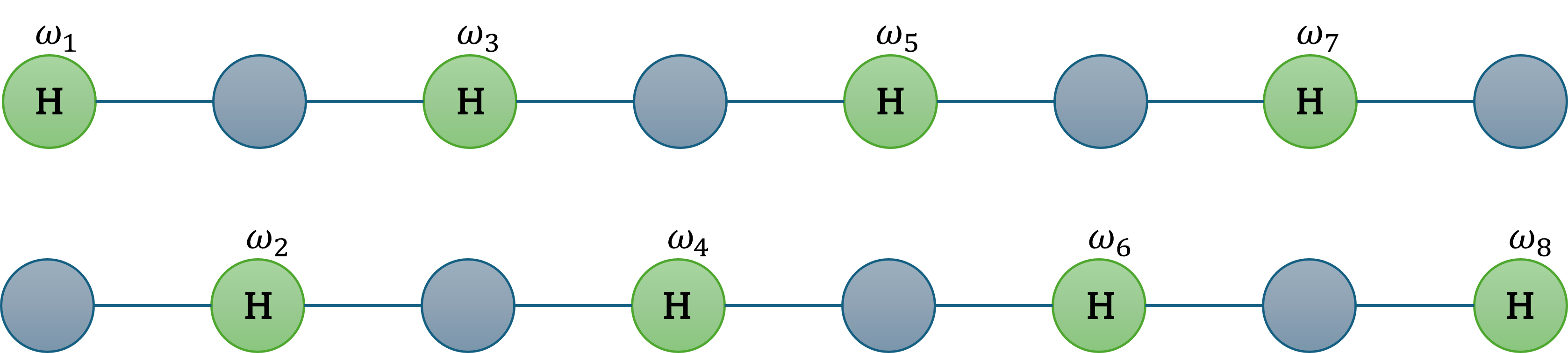
(b)

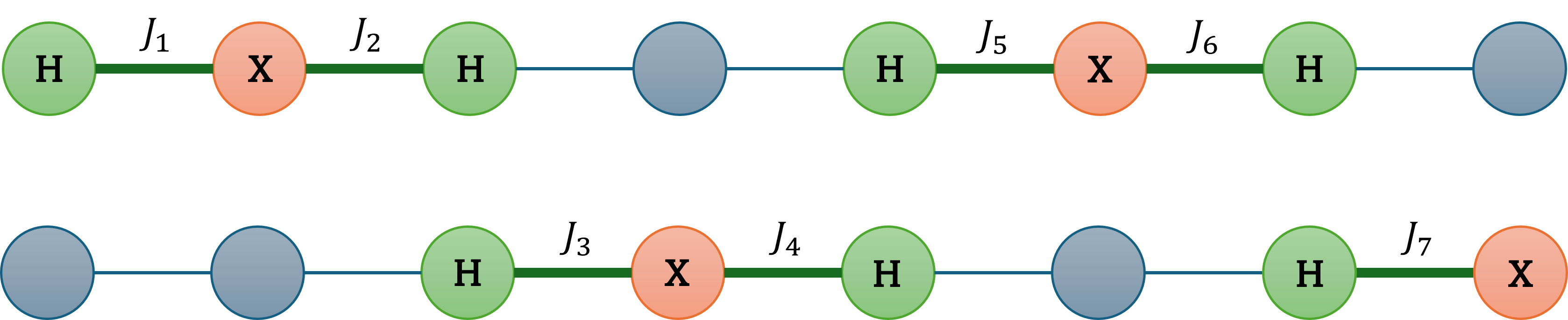
Figure 4: Schematic representation of the four experiments used to calibrate the multi-qubit system defined in Eq. (6): (a) two experiments are used to measure $\omega_{j}$: the green nodes represent qubits in the $|+\rangle$ state, and the blue nodes represent qubits in the $|0\rangle$ state; (b) two experiments are used to measure $J_{j}$: the red nodes represent qubits in the $\ket{1}$, the green nodes represent qubits in the $\ket{+}$ state, and the blue nodes represent qubits in the $\ket{0}$ state. The green edges are the measured crosstalk.

We conclude the analysis of the single-qubit case by presenting the results of an experiment using a single NV center (see SM3 for raw data). The experimental results of a Ramsey interference experiment were fit using the curves $X(t)=A\cos(\omega t+\phi)e^{-\gamma t}+B$. We first determined the “ground truth” values of all parameters using a long measurement with $N_{\rm shots}=10^{5}$ and $N_{\rm times}=100$. Next, to allow a direct comparison between the three strategies reported here, we fixed $A$, $B$ and $\phi$ to their “true” values and determined $\omega$ and $\gamma$ from a random downsampling of the experimental measurements, with up to $N_{\rm tot}=5\times 10^{5}$. Alternatively, one could extend our approach by using the Fisher Information to find the optimal strategy to probe all five fitting parameters. The experimental results, shown in Fig. 3 confirm our theoretical predictions for the comparison between the three strategies .

We now move to the systems of coupled qubits relevant to quantum computers. We consider a canonical model describing the interactions between qubits as a static crosstalk $ZZ$ term mundada2019suppression ; ni2022scalable ; xie2022suppressing ; heng2024estimatingeffectcrosstalkerror ; fors2024comprehensiveexplanationzzcoupling . For simplicity, we consider a one-dimensional chain described by

$$H=\sum_{i=1}^{N_{\rm qubits}}\left[\frac{\omega_{i}}{2}+h_{i}(t)\right](1-Z_{i})+\frac{J_{i}}{4}(1-Z_{i})(1-Z_{i+1})$$ (6)

The crosstalk couplings $J_{i}$ effectively shift the frequency of the $i$th qubit if the $i+1$th qubit is in the $|1\rangle$ ($Z_{i+1}=-1$) state, and vice versa. Importantly, Eq. (6) is diagonal in the Z basis and can be solved analytically for any initial state.

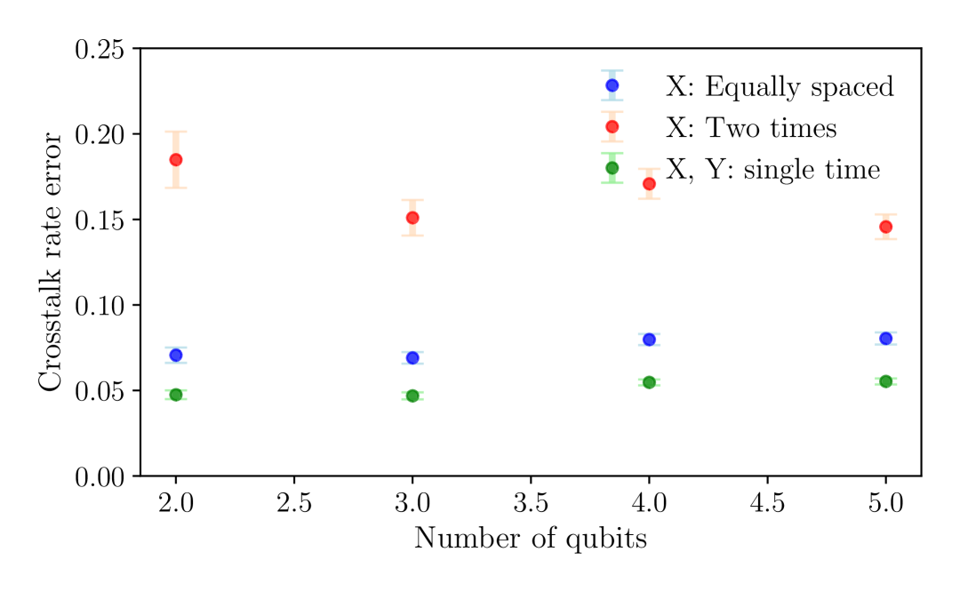
Figure 5: Numerical simulation of crosstalk-rate error as a function of the number of qubits. The parameters were sampled from a normal distribution $\omega,\gamma\in N(1,0.2),J\in N(0.5,1)$. The simulation used the protocols described in fig. 4.

A naive approach to the problem of calibrating the system described by Eq. (6) consists of preparing all qubits in the $|+\rangle$ state and performing simultaneous Ramsey interference experiments. By fitting the resulting $X_{i}(t)$ and $Y_{i}(t)$ to the theoretical curves, one can estimate all the parameters. While this approach is formally correct, we found that it is not optimal, due to the complex shape of the resulting analytical functions, and generically leads to errors that are one order of magnitude larger than the optimal ones, see SM5.

Our proposed strategy for computing the values of $\omega_{i}$ and $J_{i}$ involves reducing the many-body problem to that of isolated single qubits. Specifically, we propose to perform two pairs of experiments, respectively, to probe the detunings and the crosstalk couplings, see Fig. 4 for details. Each experiment involves a Ramsey interference experiment on half of the qubits (denoted by “H”), for different initial states of the other qubits. In the former two experiments, the qubits rotate at frequency $\omega_{i}$, while in the latter two, they rotate at frequency $\omega_{i}+J_{i\pm 1}$. The numerical results of this approach are presented in Fig. 5 and demonstrate the scalability of our protocol, as the error is essentially independent of the system size. Measuring both X and Y is optimal in this problem as well.

This approach can be straightforwardly extended to quantum computers with a more complex connectivity between the qubits. In general, the number of experiments needed to calibrate the system depends on the amount of non-negligible crosstalk couplings per qubit. For bipartite lattices with nearest-neighbor couplings, it is easy to see that one can determine all the systems’ parameters using the same four experiments as in the one-dimensional case. Interestingly, for IBM’s heavy-hex topology, it can be shown that four experiments are also sufficient, as seen in SM6. For more complex topologies, the problem at hand can be formulated as a tiling optimization problem, which can be solved heuristically and warrants further investigation.

We demonstrated the feasibility of this approach by calibrating the crosstalk coupling between two transmon qubits in the Gilboa superconducting quantum computer iqcc , with up to $N_{\rm times}=30$ and $N_{\rm shots}=20000$ (see SM3 for raw data). The experimental results are shown in shown Fig. 3(b) and demonstrate two separate regimes: for $N_{\rm tot}<10^{3}$, the curves follow our theoretical modelling, while for larger $N_{\rm tot}$ measurements based on one or two times saturate to a value that is different than the one obtained by using all measurement times. This discrepancy indicates that the experiment deviates from our simple-minded theoretical model and can be fixed by considering more realistic theoretical models, for example, affected by quasiparticle fluctuations serniak2018hot ; landa2023nonlocal , which go beyond the scope of the present analysis.

In summary, this article proposes and validates optimal strategies for characterizing qubit detuning and crosstalk in superconducting quantum computers. While traditional methods spread measurements across multiple times to average out noise, our work demonstrates that concentrated, optimally-timed measurements can achieve better results with fewer resources. By analyzing different measurement protocols using the Fisher information framework and the Cramér–Rao bound, we demonstrated that measurements of both X and Y quadratures at a single optimal time yields the best precision and resilience to parameter variation. We then extended our analysis to multi-qubit systems, where we described a method that effectively reduces the estimation of crosstalk terms to decoupled single-qubit problems, drastically simplifying calibration. Our framework scales well to larger systems and complex architectures, making it highly relevant for current and future quantum processors. Experimental validation and simulations confirm that the proposed strategies can cut calibration time by up to 50% without compromising accuracy. Looking forward, integrating these optimized calibration strategies into real-time control systems could significantly enhance the stability and scalability of quantum computing platforms.

Supplemental Materials

I Number of shots per measurement time

In this work, we utilize the Fisher information to determine the optimal strategy for performing a Ramsey interference experiment. To find this strategy, we assume that the measurement scheme includes $N_{\rm times}$ measurements at times $T=(t_{1},...,t_{N_{\rm times}})$, each with a different number of shots $S=(s_{1},...,s_{N_{\rm times}})$. We then optimize the Cramér-Rao bound (CRB) with respect to both $T$ and $S$, while keeping a total number of shots $\sum_{i}s_{i}=N_{\rm tot}$. Finally, we inspect the final result and, whenever two times are closer than an arbitrarily small margin, we merge them into a single time.

Algorithm 1 Optimal Allocation of Measurement Times and Shots

0: Maximal number of measurement times $N_{\rm times}$ (default $N_{T}=10$)

0: Total shots $N_{\rm tot}$ (default $1000$)

0: Merge tolerance $\delta$ (default $0.01$)

0: Optimised times and shots $(\widehat{T},\widehat{S})$

1: Optimise:  $\displaystyle(\widehat{T},\widehat{S})=\arg\min_{\{t_{i},s_{i}\}}\bigl{[}\,\mathrm{CRB}_{\omega}(T,S)+\,\mathrm{CRB}_{\gamma}(T,S)\bigr{]}$   s.t. $\sum_{i}s_{i}=N_{\rm tot},\;s_{i}\in\mathbb{N}_{\geq 0},\;t_{i}>0$

2: Group: merge any two times with $|t_{i}-t_{j}|<\delta$   by $\;(t_{i},t_{j})\!\longrightarrow\!\bigl{(}(t_{i}+t_{j})/2\bigr{)}$ and $(s_{i},s_{j})\!\longrightarrow\!s_{i}+s_{j}$.

3: return  $(\widehat{T},\widehat{S})$

In all cases we considered, the algorithm converged to two measurement times only, consistently with the number of free parameters in the theoretical result (see Fig. 6 for an example). In contrast, the number of shots in each measurement depended on $\omega$ and $\gamma$. Figure 7 shows the ratio of the number of measurements between the first and second time as a function of $\gamma/\omega$. The ratio changes from approximately one for $\gamma<\omega$ to 0.6 for $\gamma=3\omega$. Intuitively, for large values of $\gamma$, later times provide less information about the system, and are probed with a smaller number of shots. To simplify our presentation, in the main text, we fixed this ratio to 1, such that both times are measured with the same number of shots.

(a)

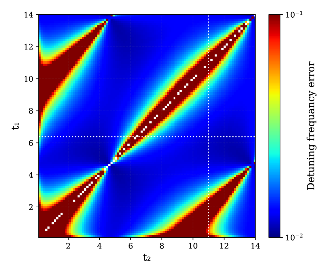
(b)

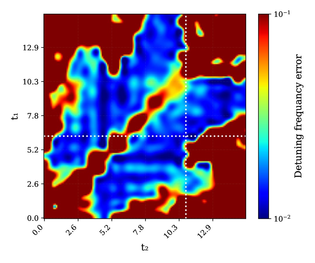
Figure 6: Cramér-Rao bound as a function of the measurement times in (a) the theoretical calculation and (b) IQCC experiment (IQCC), for $\omega=0.34$ and $\gamma=0.135$. The dashed lines denote the optimal times.

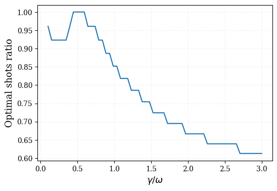
Figure 7: Ratio of the number of shots between the first and second measurements, as a function of $\gamma/\omega$. The discrete steps are related to the total number of measurements used in the optimization algorithm: the curve becomes continuous for $N_{\rm shots}\to\infty$.

II Derivation of Eq. (5) for the Cramér-Rao bound in the Gaussian approximation.

Under the Gaussian approximation, the result of each measurement is given by the normal distribution

$$x_{n}\;\sim\;\mathcal{N}\!\bigl{(}\expectationvalue{X(t_{n})},\,\sigma^{2}\bigr{)}.$$ (7)

In this case, the likelihood and log-likelihood functions are respectively defined by

$$L(\bm{\theta}) =\prod_{n=1}^{N}\frac{1}{\sqrt{2\pi\sigma^{2}}}\,\exp\!\Bigl{[}-\tfrac{\bigl{(}x_{n}-\expectationvalue{X(t_{n})}\bigr{)}^{2}}{2\sigma^{2}}\Bigr{]}$$ (8)

$$=(2\pi\sigma^{2})^{-N/2}\,\exp\!\Bigl{[}-\frac{1}{2\sigma^{2}}\sum_{n=1}^{N}\bigl{(}x_{n}-\expectationvalue{X(t_{n})}\bigr{)}^{2}\Bigr{]}$$ (9)

and

$$\ell(\bm{\theta})=\ln L(\bm{\theta})=-\frac{N}{2}\ln\!\bigl{(}2\pi\sigma^{2}\bigr{)}-\frac{1}{2\sigma^{2}}\sum_{n=1}^{N}\bigl{(}x_{n}-\expectationvalue{X(t_{n})}\bigr{)}^{2}.$$ (10)

By differentiating $l$ with respect to the fit parameters $\theta_{i}$, we obtain

$$\partialderivative{\ell}{\theta_{j}}=\frac{1}{\sigma^{2}}\sum_{n=1}^{N}\bigl{(}x_{n}-\expectationvalue{X(t_{n})}\bigr{)}\,\partialderivative{\expectationvalue{X(t_{n})}}{\theta_{j}}.$$ (11)

By definition, the Fisher information is given by

$$\mathcal{I}_{jk}(\bm{\theta})=\mathbb{E}\!\quantity[\partialderivative{\ell}{\theta_{j}}\,\partialderivative{\ell}{\theta_{k}}]$$ (12)

and equals

$$\mathcal{I}_{jk}(\bm{\theta}) =\frac{1}{\sigma^{4}}\sum_{n=1}^{N}\sum_{m=1}^{N}\underbrace{\mathbb{E}\!\quantity[\bigl{(}x_{n}-\expectationvalue{X(t_{n})}\bigr{)}\bigl{(}x_{m}-\expectationvalue{X(t_{m})}\bigr{)}]}_{\displaystyle\sigma^{2}\,\delta_{nm}}\partialderivative{\expectationvalue{X(t_{n})}}{\theta_{j}}\,\partialderivative{\expectationvalue{X(t_{m})}}{\theta_{k}}$$ (13)

$$=\frac{1}{\sigma^{4}}\sum_{n=1}^{N}\sigma^{2}\,\partialderivative{\expectationvalue{X(t_{n})}}{\theta_{j}}\,\partialderivative{\expectationvalue{X(t_{n})}}{\theta_{k}}$$ (14)

$$=\frac{1}{\sigma^{2}}\sum_{n=1}^{N}\partialderivative{\expectationvalue{X(t_{n})}}{\theta_{j}}\,\partialderivative{\expectationvalue{X(t_{n})}}{\theta_{k}}.$$ (15)

III Raw data from experimental systems

To benchmark our optimization strategies, we performed Ramsey-interference measurements on a superconducting transmon and an NV centre. Fig. 8 shows representative raw traces together with damped‑cosine fits, from which we extract the “true” parameters used to compare estimation errors.

(a)

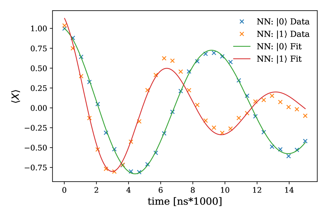
(b)

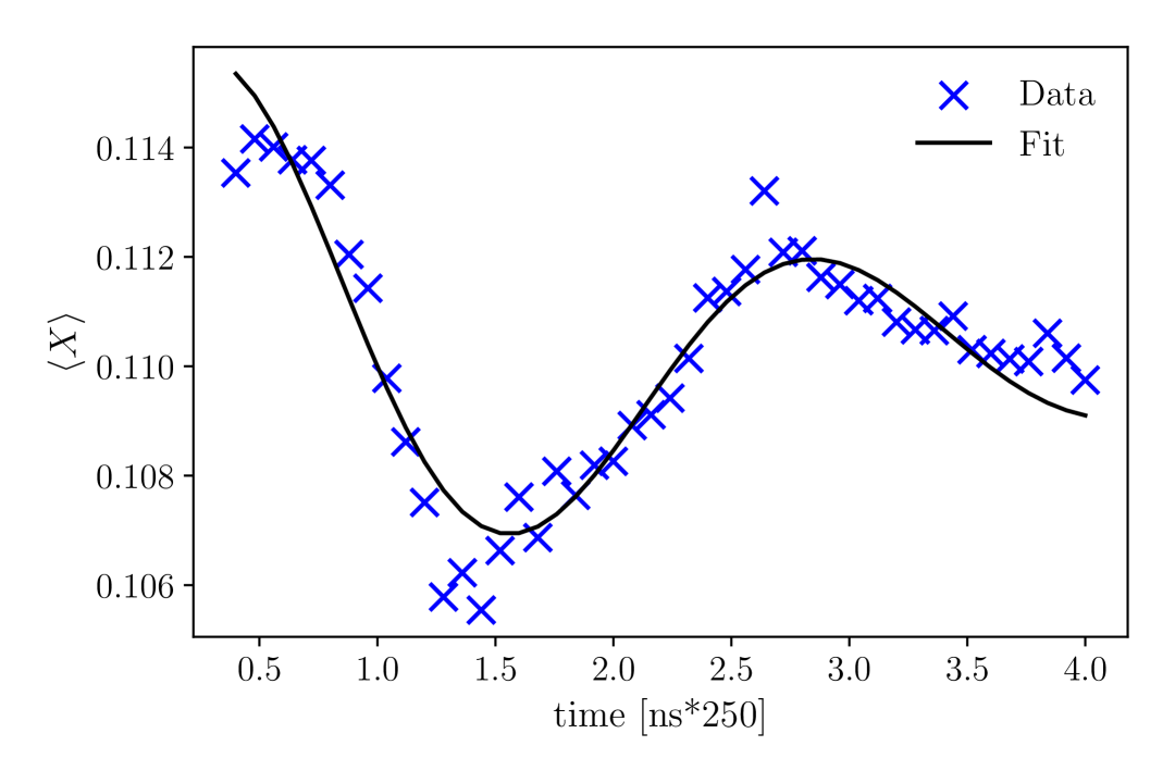
Figure 8: Raw Ramsey‑interference data (crosses) and least‑squares fits to $A\cos(\omega t+\phi)\,e^{-\gamma t}+c$ (solid lines). (a) Superconducting circuit: $\langle X\rangle$ vs. time$[\mathrm{ns}\!\times\!1000]$ for a target qubit whose nearest neighbour (NN) is prepared in $\ket{0}$ (blue/green) or $\ket{1}$ (orange/red), revealing a state‑dependent frequency shift (crosstalk). (b) NV centre: $\langle X\rangle$ vs. time$[\mathrm{ns}\!\times\!250]$. The extracted fit parameters serve as ground truth for error estimation.

IV Optimal measurement time for the X, Y strategy

In the case of measuring X and Y at a single time, one can find the optimal time analytically:

$$\mathcal{I}_{\omega\omega} =\frac{1}{\sigma^{2}}\Bigl{[}\bigl{(}-t\,e^{-\gamma t}\sin(\omega t)\bigr{)}^{2}+\bigl{(}-t\,e^{-\gamma t}\cos(\omega t)\bigr{)}^{2}\Bigr{]}=\frac{t^{2}e^{-2\gamma t}}{\sigma^{2}}\bigl{[}\sin^{2}(\omega t)+\cos^{2}(\omega t)\bigr{]}=\frac{t^{2}e^{-2\gamma t}}{\sigma^{2}},$$ (16)

$$\mathcal{I}_{\gamma\gamma} =\frac{1}{\sigma^{2}}\Bigl{[}\bigl{(}-t\,e^{-\gamma t}\cos(\omega t)\bigr{)}^{2}+\bigl{(}t\,e^{-\gamma t}\sin(\omega t)\bigr{)}^{2}\Bigr{]}=\frac{t^{2}e^{-2\gamma t}}{\sigma^{2}}\bigl{[}\cos^{2}(\omega t)+\sin^{2}(\omega t)\bigr{]}=\frac{t^{2}e^{-2\gamma t}}{\sigma^{2}},$$ (17)

$$\mathcal{I}_{\omega\gamma} =\frac{1}{\sigma^{2}}\Bigl{[}\bigl{(}-t\,e^{-\gamma t}\sin(\omega t)\bigr{)}\bigl{(}-t\,e^{-\gamma t}\cos(\omega t)\bigr{)}+\bigl{(}-t\,e^{-\gamma t}\cos(\omega t)\bigr{)}\bigl{(}t\,e^{-\gamma t}\sin(\omega t)\bigr{)}\Bigr{]}=0$$ (18)

We find that the Fisher Information matrix is

$$\mathcal{I}(t) =\frac{t^{2}e^{-2\gamma t}}{\sigma^{2}}\begin{pmatrix}1&0\\ 0&1\end{pmatrix},$$ (19)

leading to the Cramér-Rao Bound (CRB)

$$CRB_{\theta} =\bigl{[}\mathcal{I}^{-1}(t)\bigr{]}_{jj}=\frac{\sigma^{2}e^{2\gamma t}}{t^{2}}\qquad(\theta=\omega,\gamma),\qquad(j=1,2).$$ (20)

To optimize the CRB we take a derivative with respect to $t$ of the function $f(t):={e^{2\gamma t}}/{t^{2}}$ and demand it to be equal to zero: $f^{\prime}(t)={e^{2\gamma t}}\bigl{(}2\gamma t-2\bigr{)}/t^{3}=0$, leading to

$${t_{\text{opt}}=\frac{1}{\gamma}},$$ (21)

One can check that this is indeed a maximum by taking the second derivative: $f^{\prime\prime}(t_{\text{opt}})={2e^{2}}/{t_{\text{opt}}^{4}}>0$.

V Simultaneous Ramsey interference experiment on all qubits

Theoretically, to estimate all parameters, one could initialize the entire system into a global superposition state $\ket{+}^{\bigotimes n}$, allow it to evolve over time, and subsequently measure all qubits simultaneously. The resulting data would then be fitted to the analytical model to deduce the system’s parameters, including both individual qubit detunings and crosstalk effects. In practice, this is not so simple. To get a sense of the complexity of the problem, let us find the $\langle X\rangle$ value of the middle qubit in a simple one-dimensional 3-qubit model that is initiated in a global superposition:

$$\psi(t) = e^{-iHt}|+++\rangle,$$ (22)

$$\langle\psi(t)|IXI|\psi(t)\rangle = \frac{1}{4}\Big{(}\cos(t\omega_{i+1})+\cos(t(j_{i}+\omega_{i+1}))$$

$$\quad+\cos(t(j_{i+1}+\omega_{i+1})) + \cos(t(j_{i}+j_{i+1}+\omega_{i+1}))\Big{)}e^{-t\gamma_{i}}$$

After the fitting process, we are left with a set of parameters that are vastly different than the correct ones. Moreover, the loss function value is lower for the wrong parameters than for the true ones.

$$\sum{(y_{i}-f(x_{i},\theta_{wrong}))^{2}}\leq\sum{(y_{i}-f(x_{i},\theta_{correct}))^{2}}$$ (23)

where $y_{i}$ is the measured value and $f(x_{i},\theta)$ is the value of the expectation value function given a set of parameters $\theta$. Since we have a finite amount of shots, we have an inevitable uncertainty in our data that is governed by $\frac{1}{\sqrt{N}}$. This creates the problem of overfitting the noisy data to a completely different set of parameters.

This results in estimation errors approximately an order of magnitude higher than those obtained from the single-qubit methods.

VI Tiling of IBM quantum computers

In the main text, we demonstrated how to calculate the crosstalk of a one-dimensional system using two experiments. Here, we extend the same approach to the two-dimensional topology of IBM quantum computers.

(a)

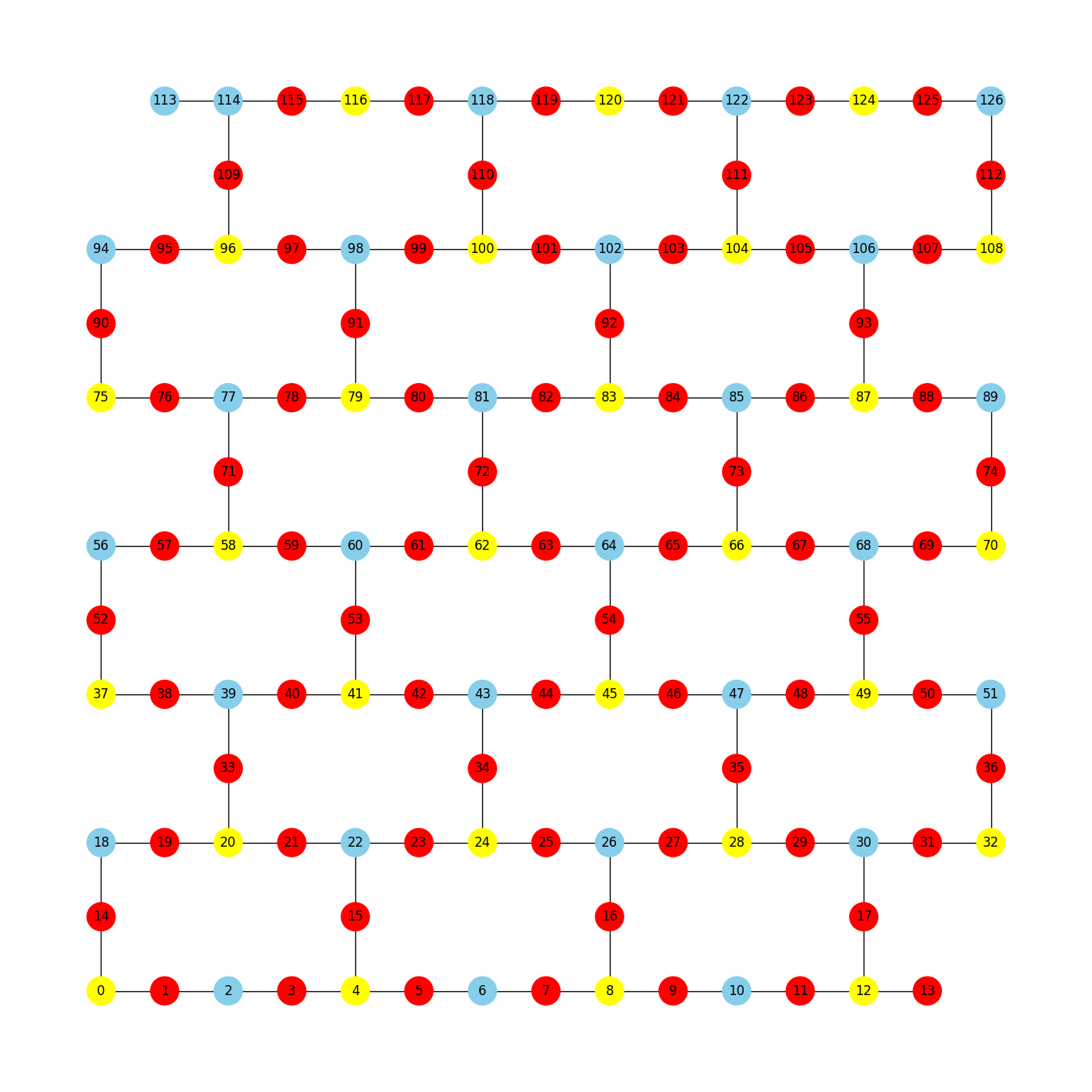
(b)

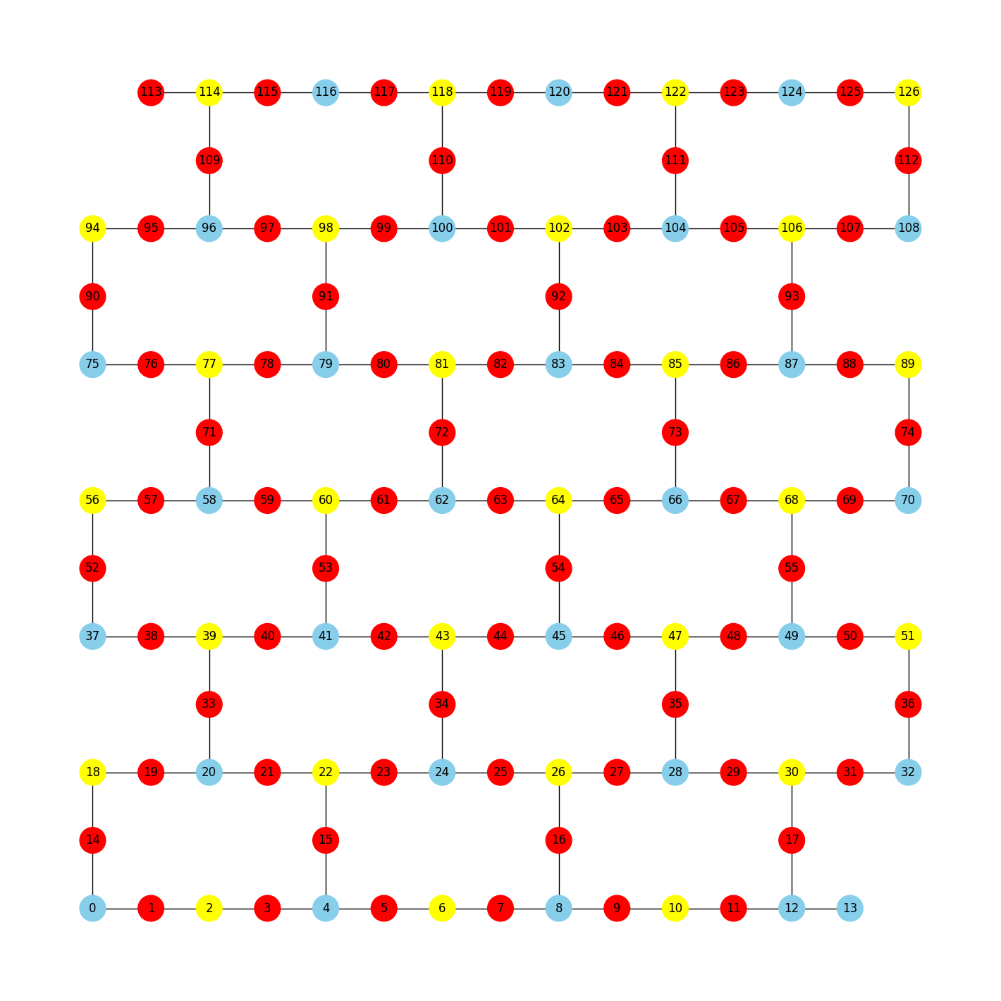
Figure 9: IBM tiling for probing crosstalk effects. The red nodes represent qubits in the $\ket{+}$ state where the Ramsey interference is performed, and blue (yellow) nodes represent qubits in the $\ket{0}$ ($\ket{1}$) state.