An Exact Gradient Framework for Training Spiking Neural Networks

Abstract

Spiking neural networks inherently rely on the precise timing of discrete spike events for information processing. Incorporating additional bio-inspired degrees of freedom, such as trainable synaptic transmission delays and adaptive firing thresholds, is essential for fully leveraging the temporal dynamics of SNNs. Although recent methods have demonstrated the benefits of training synaptic weights and delays, both in terms of accuracy and temporal representation, these techniques typically rely on discrete-time simulations, surrogate gradient approximations, or full access to internal state variables such as membrane potentials. Such requirements limit training precision and efficiency and pose challenges for neuromorphic hardware implementation due to increased memory and I/O bandwidth demands. To overcome these challenges, we propose an analytical event-driven learning framework that computes exact loss gradients not only with respect to synaptic weights and transmission delays but also to adaptive neuronal firing thresholds. Experiments on multiple benchmarks demonstrate significant gains in accuracy (up to $7\%$), timing precision, and robustness compared to existing methods.

I Introduction

Spiking neural networks (SNNs), often described as the third generation of neural network models [1], encode and transmit information through asynchronous spike events rather than continuous-valued activations; see Fig. 1. This event-based paradigm holds great promise for energy-efficient computing, as evidenced by emerging neuromorphic hardware platforms such as SENeCa [2], Intel Loihi2 [3], and IBM TrueNorth [4], which leverage sparse spike-based communication to reduce power consumption. The inherent sparsity and binary nature of spikes significantly reduce the number of expensive arithmetic operations, and recent estimates suggest that deep SNNs could potentially achieve orders-of-magnitude energy savings over analog-valued networks under the right conditions [5].

This directly appeals to the broader design automation community, which is increasingly shifting toward bio-inspired and neuromorphic architectures that promise ultra-low-power, high-throughput computation for Artificial Intelligence (AI) workloads. By leveraging the massive parallelism and event-driven nature of SNNs, design flows can be tailored for embedded systems and IoT devices where efficiency is paramount. This effort aligns with emerging needs in autonomous robotics, real-time analytics, and next-generation cyber-physical systems.

These advances have spurred growing interest in deploying SNNs for complex tasks, and SNN models have indeed begun scaling to deeper architectures with modern features like attention mechanisms and transformer-like designs [6, 7]. Nevertheless, a persistent challenge remains: SNNs trained with current methods often underperform standard ANN counterparts on many benchmarks, particularly when constrained to similar network sizes or latencies [8]. This performance gap is primarily attributed to the difficulty of training SNNs, which stems from the non-differentiable spike generation mechanism and the resulting credit assignment problem in time.

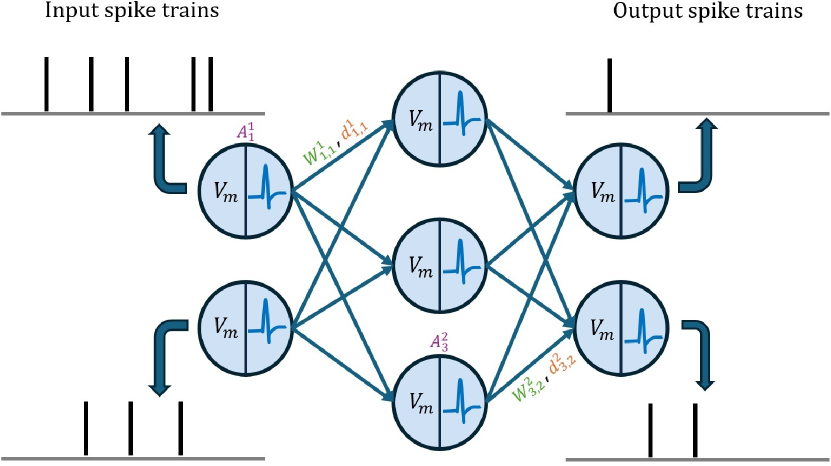
Figure 1: A schematic of a spiking neural network. $A^{l}_{i}$, $W^{l}_{ij}$, and $d^{l}_{ij}$ are trainable adaptive threshold, weight, and delay parameters.

In this paper, we advance the state of the art SNN training by introducing a comprehensive learning approach for deep spiking networks. We propose an event-driven gradient-based framework that jointly optimizes synaptic weights, heterogeneous transmission delays, and adaptive neuron thresholds in continuous time. To our knowledge, this work is the first to derive exact analytic gradients for both synaptic and intrinsic neuronal parameters in SNNs without resorting to approximation, enabling the co-learning of delays and threshold adaptation with the same level of precision as weight updates. The result is a set of update rules triggered only at event times (spikes), making the algorithm temporally and spatially sparse by design. By operating directly on spike times and inter-spike intervals, the learning rule naturally grants the network fine-grained control over spike timing relationships: adjusting a delay influences when a postsynaptic neuron receives a given presynaptic spike, while adjusting a neuron’s threshold influences whether and when it fires in response. Our experiments show that co-optimizing these parameters significantly improves performance on tasks requiring precise temporal pattern recognition and long-range temporal credit assignment, compared with SNNs that have fixed delays or non-adaptive thresholds. Furthermore, our approach retains the practical advantages of event-driven computation. Moreover, combining trainable delays with adaptive thresholds produces networks that are more robust to timing noise and parameter fluctuations, since both mechanisms can compensate by dynamically adjusting spike alignments and excitability.

Collectively, these innovations address key algorithmic and theoretical challenges in SNN training and also pave the way for highly efficient, event-driven hardware designs that fully exploit the energy benefits of spike-based computation. We envision that this framework will spur new research directions in the design automation community, bridging the gap between algorithmic innovation and large-scale, low-power neuromorphic deployment. In summary, the main contributions of this work are as follows:

1. We derive a novel event-driven learning rule that provides exact gradients for both synaptic weights and transmission delays in SNNs, extending prior continuous-time approaches and eliminating the need for surrogate gradients or dense time sampling for delay training.

2. We introduce a co-learning mechanism for adaptive neuron thresholds within the same analytical framework, allowing each neuron to learn its own excitability profile in concert with synaptic plasticity. This biologically inspired addition expands the temporal memory capacity of the network by leveraging the neuron’s internal dynamics.

3. We empirically demonstrate the benefits of jointly optimizing delays, weights, and thresholds on three sequential processing benchmarks. Our experiments show that the proposed approach achieves higher accuracy and more precise spike timing control than both weight-only and weight+delay-only training, often with fewer trainable parameters, and that it improves learning stability in the face of noise and hardware variability.

We organize the paper as follows. Section II briefly surveys some related work. In Section III, we introduce our theoretical framework and derive the exact gradient method. Next, building on this theoretical foundation, we formulate our event-driven training algorithm. In Section IV, we elaborate on the experiments and report the results. Section V finally summarizes our contribution and highlights some potential future work directions.

II Related work

Over the past few years, significant progress has been made in SNN training algorithms to surmount challenges raised due to the non-differentiable spike generation mechanism and the resulting credit assignment problem in time. A dominant approach for deep SNNs is backpropagation-through-time using surrogate gradients that smooth or approximate the discontinuous spiking function [9]. This strategy enables gradient-based optimization of SNN parameters by effectively “tricking” the optimizer into ignoring the threshold discontinuity. The surrogate gradient approach has allowed SNNs to achieve competitive accuracy in image classification and even tackle complex sequence tasks, paving the way for training SNNs with many layers [10]. Techniques such as spike-element-wise ResNets have been proposed to alleviate issues like vanishing gradients in deep SNNs [10], and researchers have successfully trained SNNs with attention layers or transformer-like architectures by carefully managing temporal credit assignment [6, 7]. Despite these advances, certain training-related compromises, such as relying on rate-based abstractions or coarse time-step approximations, often prevent SNNs from realizing the full potential of precise spike timing. In particular, most conventional SNN models still rely on a simplified abstraction of neural processing, such as static per-synapse weights and fixed neuron thresholds, with information largely encoded in spike rates or coarse spike counts. Such simplifications can limit the temporal expressiveness of SNNs, motivating research into additional trainable mechanisms that can harness fine-grained spike timing information.

One powerful yet underexplored mechanism for temporal processing in SNNs is the incorporation of synaptic transmission delays. In biological neural systems, axonal conduction delays play a critical role in coordinating spike arrival times; the myelination and length of axons cause each spike to arrive after a neuron-specific delay, affecting how downstream neurons integrate inputs [11]. These delays are known to be crucial for functions such as sound localization and sensory processing [12], and there is evidence that synaptic delays themselves can undergo activity-dependent plasticity during learning [13]. Theoretical studies have shown that even a single layer of spiking neurons with programmable input delays can handle a richer class of temporal functions than standard perceptron-like models without delays [14]. By adjusting when a spike is delivered, an SNN can align or offset spikes in time, enabling it to detect temporal coincidences and sequence patterns that would be impossible to capture with only instantaneous synaptic interactions. From another perspective, one can note that SNN links may emerge as a compelling application for asynchronous logic, as a key challenge lies in conveying analog values digitally through simple interfaces. While rate encoding is common, delay encoding offers a more energy-efficient alternative by representing values via inter-pulse delays, making delay training even more attractive [15, 16].

Despite numerous advantages, synaptic delays remain relatively underutilized in mainstream SNN training frameworks, which often assume zero or fixed transmission delays for simplicity. Some studies have explored training delays using local rules inspired by spike-timing dependent plasticity [17] or supervised schemes like ReSuMe that target desired spike times [18]. More recently, surrogate gradient methods have been extended to handle trainable delay parameters: for example, SLAYER, a spike-based backprop framework, was adapted to learn per-neuron axonal delays [19], later augmented with learnable delay caps to bound the range of delays.

Notably, recent results even suggest that in certain setups, training only the synaptic delays (while keeping weights fixed) can achieve accuracy on par with training only the weights [20], underscoring the potent computational role of timing. Still, most existing delay-learning methods rely on approximate gradients or dense time-step simulations, which can introduce precision errors and large memory overhead. There is a clear need for more exact and efficient training approaches to fully exploit synaptic delays for precision spike timing control in deep SNNs.

On the other hand, another key avenue for enhancing the temporal computing capacity of SNNs lies in adaptive neuronal thresholds and other intrinsic plasticity mechanisms. Biological neurons exhibit a variety of adaptation phenomena: after spiking, a neuron may become less excitable for a period due to ion channel dynamics, effectively raising its firing threshold or inducing an after-current. Such spike-frequency adaptation mechanisms allow neurons to adjust their responsiveness based on recent activity, introducing a longer-term state that extends beyond instantaneous membrane potential integration [21]. In practice, adaptation endows spiking neurons with an inherent memory of their past spiking, often constraining excessive firing and enabling sensitivity to input patterns over extended timescales [22].

Inspired by biology, several SNN models have incorporated adaptive thresholds or currents to improve performance on tasks requiring temporal credit assignment. For instance, an adaptive leaky integrate-and-fire neuron can be implemented by increasing its threshold each time it emits a spike and letting it decay slowly thereafter [23]. Networks of such neurons, sometimes called long short-term memory SNNs (LSNNs), have been shown to solve temporal tasks that are challenging for standard LIF networks, by retaining information over hundreds of milliseconds in the adapting threshold variable [23]. Recent studies have explored learning the parameters of these adaptation mechanisms directly: e.g., optimizing a distribution of neuron time constants or threshold reset values to balance network dynamics [10]. Other works have proposed gating or modulation of membrane parameters (such as the Gated LIF neuron) to adaptively control neuron dynamics [24]. In addition to threshold modulation, complementary adaptation models use activity-dependent hyperpolarizing currents: for example, the Adaptive LIF (AdLIF) model includes a secondary internal variable to accumulate an adaptation current triggered by spikes [25]. This approach was recently shown to outperform simple threshold adaptation on certain benchmarks.

Despite these promising findings, most previous studies address neuronal adaptation and synaptic plasticity separately. The joint optimization of synaptic delays and neuron-specific adaptation parameters in a unified learning algorithm remains largely unexplored, especially using exact gradient-based methods.

Both synaptic delays and adaptive thresholds complement each other in enriching SNN dynamics, significantly increasing temporal computing power. Delays explicitly align distant spikes in time, while adaptation implicitly adjusts a neuron’s sensitivity based on its firing history. Combined, they offer fine-grained spike timing control and distributed memory, potentially enabling SNNs to tackle previously unattainable temporal tasks. However, realizing these benefits requires handling the event-driven discontinuities of spiking across all parameters. Though surrogate gradient methods can be extended to delays and thresholds, surrogate choices and time discretization risk approximation errors and hamper precise timing. Ideally, one desires a method treating spike times as continuous variables, propagating errors precisely at spike events to directly relate delay or threshold changes to spike timing.

Recent developments in differentiable spiking neuron theory enable such exact training. Notably, [26] introduced event-based backpropagation (EventProp) for continuous-time SNNs, computing exact gradients by backpropagating errors through spike events. By accounting for discontinuities at these events, EventProp yields exact timing gradients without surrogate smoothing. Building on this, [27] proposed DelGrad, which analytically computes exact loss gradients for both weights and synaptic delays in an event-driven manner, eliminating the need to store full membrane traces and showing that trainable delays can improve accuracy and robustness in neuromorphic implementations [27]. Yet such exact gradient techniques remain unexplored for adaptive thresholds, which add further discontinuities. Merging exact event-driven gradient methods with neuron-specific adaptation offers a promising path toward jointly fine-tuning spike timing (via delays) and neuronal excitability (via thresholds/adaptation) in a single optimization framework.

Notably, researchers have already demonstrated the feasibility of training a multi-layer SNN with delays and adaptive neurons on the analog BrainScaleS-2 neuromorphic processor in a chip-in-the-loop setup, which led to a reduction in memory and communication overhead for on-chip learning. Moreover, from a system-level perspective, the chip-in-the-loop demonstration underscores the compatibility of this approach with real hardware architectures and on-chip learning engines that strictly manage memory and communication overhead. Such synergy is pivotal to cutting-edge research in bio-inspired computation, as well as in hardware systems for AI, where tightly constrained resources must be balanced against the demand for rapid, adaptive on-device inference. This opens the door to integrating event-based training algorithms into broader CAD flows, facilitating the co-design of spiking neural hardware and software for embedded, IoT, and large-scale neuromorphic applications.

III Theoretical framework

SNNs are known to be non-differentiable at moments when a neuron’s spike count changes (e.g., from $0$ to $1$ spike or from $1$ to $2$ spikes) [28]. More specifically, the spiking function is a Heaviside step (denoted by $\Theta(x)$), meaning a neuron does not fire at the subthreshold but suddenly fires a spike upon crossing a threshold value $V_{thr}$. If one treats that function as a direct $\Theta$-function, the derivative is $0$ almost everywhere and undefined at the threshold crossing.

However, the spike time $t_{j}$ can, per se, be taken into account as a continuous variable implicitly defined by $V_{j}(t_{j})=V_{thr}$. That equation is locally differentiable with respect to parameters, like weights and delays, as long as the system adheres to some mild condition (see Section III-B). In that case, we can regard $t_{j}$ as a continuously varying variable with respect to parameters. In essence, SNNs can be considered piecewise differentiable: within a regime in which each neuron emits a fixed number of spikes, those spike times can be treated as continuous, implicit variables. Crucially, within a stable spiking regime, where the count and ordering of spikes are not changing under small parameter perturbations, the function is indeed differentiable. This is precisely the domain in which we aim to propose our implicit differentiation.

III-A Spiking neuron model with delays

We focus on a Leaky Integrate-and-Fire (LIF) neuron, closely aligned with Loihi’s default on-chip neuron model. For a post-synaptic neuron $j$, its subthreshold membrane potential $V_{j}(t)$ evolves according to

$$\tau_{m}\frac{dV_{j}(t)}{dt}=-\bigl{(}V_{j}(t)-V_{\text{rest}}\bigr{)}+\sum_{i}w_{ij}\,S_{i}\bigl{(}t-d_{ij}\bigr{)},$$ (1)

where $\tau_{m}$ is the membrane time constant, $V_{\text{rest}}$ is the resting potential (often taken as $0$ for simplicity), $w_{ij}$ is the synaptic weight from pre-synaptic neuron $i$ to $j$, and $S_{i}(t)$ is the spike train of neuron $i$, typically represented as $S_{i}(t)=\sum_{f}\delta\bigl{(}t-t_{i}^{(f)}\bigr{)}$ where $t_{i}^{(f)}$ is the $f$-th spike time of neuron $i$ and Dirac delta $\delta(\cdot)$ is used to represent an instantaneous spike at exactly $t_{i}^{(f)}$. The term $d_{ij}$ represents the integer (or real) delay between neuron $i$ firing and neuron $j$ receiving that spike. This means that if $i$ fires at $t_{i}^{(f)}$, then $j$ sees that spike at $t_{i}^{(f)}+d_{ij}$. Having this considered, Eq. 1 turns into

$$\tau_{m}\frac{dV_{j}(t)}{dt}=-\bigl{(}V_{j}(t)-V_{\text{rest}}\bigr{)}+\sum_{i}\sum_{f}w_{ij}\,\delta\bigl{(}t-[t_{i}^{(f)}+d_{ij}])\bigr{)}.$$ (2)

Neuron $j$ emits a spike whenever $V_{j}(t)$ crosses the threshold $V_{\text{thr}}$. After firing, $V_{j}$ is reset to (or clamped at) $V_{\text{rest}}$ for a refractory period. Here, for the sake of theoretical clarity, we focus on the timing of the first spike event in a given time window and ignore subsequent spikes. Extensions to multiple spikes are straightforward but require summation across spikes. If neuron $j$ fires once at time $t_{j}$, the condition is:

$$V_{j}(t_{j})=V_{\text{thr}}\quad\text{and}\quad\frac{dV_{j}}{dt}\Bigl{|}_{t=t_{j}}>0,$$ (3)

which implies that the membrane potential just reaches threshold from below. This equation implicitly defines $t_{j}$ as a function of the synaptic parameters $\{(w_{ij},d_{ij})\}_{i}$ and the pre-synaptic spike times $\{t_{i}^{(f)}\}_{i}$.

In fact, at the spike time $t_{j}$, the voltage is equal to $V_{thr}$, meaning the neuron firing time can be explicitly described by this crossing time $t_{j}$. Interestingly, Eq. 3 allows us to treat $t_{j}$ as an implicit function of any parameters that affect $V_{j}$, such as synaptic weights or delays. Informally speaking, delay $d_{ij}$ can dramatically alter when $j$ crosses the threshold. Small changes in $d_{ij}$ may shift the arrival of a crucial spike, strengthening or weakening its temporal overlap with other concurrent inputs. If two key inputs arrive more coincidentally, $j$ may reach threshold earlier or with fewer total spikes required. Conversely, large mismatches in arrival times can prevent $j$ from firing altogether. Thus, precisely tuning delays can endow an SNN with a refined handle on temporal pattern processing. Fig. 2 illustrates this effect.

Having this said, note that Eq. 2 is a first-order ODE in $V_{j}$ and is a compact form of expressing that the net input current is a sum of impulses from each spike since, in standard LIF, an impulse is $\delta(t-[t_{i}^{(f)}+d_{ij}])$. A well-known technique for linear ODEs with impulse (Dirac $\delta$) inputs is to use the Green’s function. Having considered that the subthreshold voltage response is often modeled by an exponential decay [29], one can solve the ODE piecewise to get a closed-form expression for $V_{j}(t)$ as the sum of exponentials $\omega(\cdot)$ with ignoring the threshold resets. That is to say, by integrating both sides of the ODE from some initial time $0$ to $t$, each delta $\delta(t-[t_{i}^{(f)}+d_{ij}])$ contributes a kick at $t=t_{i}^{(f)}+d_{ij}$. That kick in a linear first-order system produces a piecewise exponential shape $\omega(t-[t_{i}^{(f)}+d_{ij}])$. Formally speaking,

$$V_{j}\bigl{(}t,\texttt{ParamSet}=\{w_{ij},d_{ij}\}\bigr{)}=V_{\text{rest}}+\sum_{i,f}w_{ij}\cdot\omega\bigl{(}(t-[t_{i}^{(f)}+d_{ij}]\bigr{)}\text{}.$$ (4)

More specifically, considering a single delta input at time $t_{0}$ acts like an impulse driving the LIF. The subthreshold solution for an impulse at time $0$, with some membrane time constant $\tau_{m}$, typically yields a post-synaptic potential (PSP) kernel $\epsilon(\tau)$. In particular, whereas in $\delta$ input viewpoint, the forcing term in the ODE is a sum of $\delta$-functions, in the PSP kernel view, we store the result of each $\delta$-function input in memory as an $\epsilon$-shaped PSP. Mathematically, the $\delta$-function and the $\epsilon$ kernel are tied by convolution (i.e., $\epsilon(t)=\int_{0}{t}e^{-(t-\tau)/\tau_{m}}\delta(\tau)d\tau$). For a simple LIF with instantaneous synapses, one often obtains:

$$\epsilon(\tau)=\begin{cases}e^{-\tau/\tau_{m}}&\ \ \tau\geq 0\\ 0&\ \ \tau<0\end{cases}$$

plus possibly a multiplicative factor to account for the exact scaling. This kernel $\epsilon$ is the “shape” of the voltage deflection after a single instantaneous spike at time $0$, ignoring threshold and reset.

Expressing $V_{j}$ as Eq. 4 indeed facilitates the required differentiation we delve into in Section III-B, as we can start from the explicit sum of kernels form and do a straightforward partial derivative of each $\epsilon(\cdot)$ term.

III-B Exact gradient of the Loss w.r.t. delays

III-B1 Implicit differentiation of spike times

When training an SNN, one typically defines a global loss function $L$ reflecting how well the network performs on some task. For instance, if the network must classify inputs, $L$ might measure cross-entropy between the desired label and the output derived from spike timing in the output layer. Or if the network must match a desired spike train, $L$ might be the sum of squared differences between actual spike times and target spike times. Regardless, in a feedforward SNN, the only “outputs” are spike times (and possibly firing rates, but firing rates, in turn, can be functions of spike times). Consequently, one can view the entire network’s behavior as determined by the set of spike times $\{t_{k}\}$. Formally, we can write:

$$L=L\bigl{(}\{t_{k}\}\bigr{)}\quad\text{with}\quad t_{k}=f(\text{parameters}),$$

where $\{t_{k}\}$ are spike times throughout the network, including $t_{j}$. Now, from the threshold condition Eq. 3, we have

$$V_{j}\bigl{(}t_{j}(\theta),\theta\bigr{)}-V_{\text{thr}}=0.$$ (5)

Note that since each $t_{j}(\theta)$, where $\theta$ is a placeholder for parameters (weights, delays, etc.), is an implicit function, the Implicit Function Theorem [30] states $t_{j}(\theta)$ is differentiable w.r.t. $\theta$ provided that: $i)$ $V_{j}$ is continuous and differentiable w.r.t. $\theta$ and $t$ in the region, where the spiking pattern (the number/order of spikes) does not change abruptly, and $ii)$ $\frac{\partial}{\partial t}V_{j}(t_{j}(\theta))\not=0$ at the crossing time (meaning the membrane potential is strictly increasing or decreasing through threshold).

Given this, and particularly taking the delay into account, the chain rule implies the following:

$$\frac{\partial L}{\partial d_{ij}}=\frac{\partial L}{\partial t_{j}}\,\frac{\partial t_{j}}{\partial d_{ij}}+\sum_{m\neq j}\frac{\partial L}{\partial t_{m}}\,\frac{\partial t_{m}}{\partial d_{ij}}.$$

Here, $\partial t_{m}/\partial d_{ij}$ can be nonzero if neuron $m$ is downstream from $j$, meaning that $m$’s spike time depends on $j$’s spike time, which in turn depends on $d_{ij}$. This leads to a backpropagation of timing errors through the network (see Section III-B2). Here, we first focus on $\partial t_{j}/\partial d_{ij}$, the direct sensitivity of neuron $j$’s own spike time to the delay $d_{ij}$: differentiating both sides of Eq. 5 w.r.t. $d_{ij}$ and applying the chain rule gives:

Figure 2: The neuron fires at time $t_{j}$ when $V_{j}(t_{j})$ reaches the dashed threshold line. A change in delays shifts the postsynaptic crossing time, which in turn informs the gradient for backpropagation in an event-driven SNN. Decreasing the delay $d_{ij}$ raises $V_{j}$, so the threshold is reached slightly earlier ($t_{j}-\Delta t_{j}$), leading to a shift in spike time. A similar effect occurs if you increases the weight.

$$\frac{\partial}{\partial d_{ij}}\Bigl{[}V_{j}\bigl{(}t_{j}(d_{ij}),d_{ij}\bigr{)}-V_{\text{thr}}\Bigr{]}=$$

$$\quad\frac{\partial V_{j}\bigl{(}t_{j}(d_{ij}),d_{ij}\bigr{)}}{\partial d_{ij}}+\frac{\partial V_{j}\bigl{(}t_{j}(d_{ij}),d_{ij}\bigr{)}}{\partial t_{j}}\,\frac{\partial t_{j}}{\partial d_{ij}}=0.$$

This immediately results in

$$\frac{\partial t_{j}}{\partial d_{ij}}=-\displaystyle\frac{\partial V_{j}\bigl{(}t_{j}(d_{ij}),d_{ij}\bigr{)}}{\partial d_{ij}}/\displaystyle\frac{\partial V_{j}\bigl{(}t_{j}(d_{ij}),d_{ij}\bigr{)}}{\partial t_{j}}.$$ (6)

The two partial derivatives in the numerator and denominator encapsulate how $V_{j}$ depends on delay $d_{ij}$ and on time $t_{j}$ (see Fig. 2). The following lemmas will determine these terms.

Lemma 1.

$\frac{\partial V_{j}\bigl{(}t_{j}(d_{ij}),d_{ij}\bigr{)}}{\partial d_{ij}}=-w_{ij}\sum_{f}\epsilon^{\prime}\bigl{(}t-[t_{i}^{(f)}+d_{ij}]\bigr{)}.$

Proof.

In Eq. 4, in the sum for $V_{j}(t)$, only the terms involving synapse $(i,j)$ will depend on $d_{ij}$. For the other ($k\not=i$) synapses, $d_{kj}$ is unaffected. Hence:

$$\frac{\partial V_{j}\bigl{(}t_{j}(d_{ij}),d_{ij}\bigr{)}}{\partial d_{ij}}= \sum_{f}\frac{\partial}{\partial d_{ij}}\Bigl{[}w_{ij}\cdot\omega\bigl{(}t-[t_{i}^{(f)}+d_{ij}]\bigr{)}$$

$$+\underbrace{(\text{no contribution from}\ k\not=i)}_{=0}.$$

By factoring out the constant weight $w_{ij}$, we get

$$\frac{\partial V_{j}\bigl{(}t_{j}(d_{ij}),d_{ij}\bigr{)}}{\partial d_{ij}}=w_{ij}\sum_{f}\frac{\partial}{\partial d_{ij}}\Bigl{[}\omega\bigl{(}t-[t_{i}^{(f)}+d_{ij}]\bigr{)}\bigr{]}.$$ (7)

Now denote $g(d_{ij})$ by $\omega\bigl{(}t-[t_{i}^{(f)}+d_{ij}]\bigr{)}$. Letting $u=t-[t_{i}^{(f)}+d_{ij}]$ leads to $g(d_{ij})=\epsilon(u)$, which by applying the chain rule gives us

$$\frac{\partial g}{\partial d_{ij}}=\epsilon^{\prime}(u)\frac{\partial u}{\partial d_{ij}}=\epsilon^{\prime}(t-[t_{i}^{(f)}+d_{ij}])\times\frac{\partial}{\partial d_{ij}}\bigl{(}t-[t_{i}^{(f)}+d_{ij}]\bigr{)},$$

where $\epsilon^{\prime}$ is the time derivative of the PSP kernel. But

$$\frac{\partial}{\partial d_{ij}}\bigl{(}t-[t_{i}^{(f)}+d_{ij}]\bigr{)}=-1,$$

because $t$ and $t_{i}^{(f)}$ are constant w.r.t. $d_{ij}$. Hence:

$$\frac{\partial}{\partial d_{ij}}\epsilon\bigl{(}t-[t_{i}^{(f)}+d_{ij}]\bigr{)}=-\epsilon^{\prime}(t-[t_{i}^{(f)}+d_{ij}]).$$ (8)

By combining Eq. 8 into Eq. 7, we get

$$\frac{\partial V_{j}\bigl{(}t_{j}(d_{ij}),d_{ij}\bigr{)}}{\partial d_{ij}}=-w_{ij}\sum_{f}\epsilon^{\prime}\bigl{(}t-[t_{i}^{(f)}+d_{ij}]\bigr{)}.$$

Finally, to derive $\frac{\partial V_{j}\bigl{(}t_{j}(d_{ij}),d_{ij}\bigr{)}}{\partial d_{ij}}$ at the firing time $t=t_{j}$, we can jsut plug in $t_{j}$:

$$\frac{\partial V_{j}\bigl{(}t_{j}(d_{ij}),d_{ij}\bigr{)}}{\partial d_{ij}}=-w_{ij}\sum_{f}\epsilon^{\prime}\bigl{(}t_{j}-[t_{i}^{(f)}+d_{ij}]\bigr{)}.$$

∎

Lemma 2.

$\frac{\partial V_{j}\bigl{(}t_{j}(d_{ij}),d_{ij}\bigr{)}}{\partial t_{j}}=\sum_{i,f}w_{ij}\,\epsilon^{\prime}\!\bigl{(}t_{j}-[t_{i}^{(f)}+d_{ij}]\bigr{)}.$

Proof.

Similarly, increasing $t_{j}$ by a small amount $\Delta t_{j}$ means we are evaluating $V_{j}$ at a slightly later time. Intuitively, if $t_{j}$ is later, more of the preceding PSP contributions may have decayed, so $\partial V_{j}\bigl{(}t_{j}(d_{ij}),d_{ij}\bigr{)}/\partial t_{j}$ usually involves $\epsilon^{\prime}(t_{j}-[t_{i}^{(f)}+d_{ij}])$ with a positive sign. In fact, for a standard LIF or current-based model:

$$\frac{\partial V_{j}\bigl{(}t_{j}(d_{ij}),d_{ij}\bigr{)}}{\partial t}=\sum_{i,\,f}w_{ij}\,\epsilon^{\prime}\bigl{(}t-[t_{i}^{(f)}+d_{ij}]\bigr{)}.$$

Evaluated at $t=t_{j}$, this becomes

$$\frac{\partial V_{j}\bigl{(}t_{j}(d_{ij}),d_{ij}\bigr{)}}{\partial t_{j}}=\sum_{i,f}w_{ij}\,\epsilon^{\prime}\!\bigl{(}t_{j}-[t_{i}^{(f)}+d_{ij}]\bigr{)}.$$ (9)

∎

Conclusion III.1.

$\frac{\partial t_{j}}{\partial d_{ij}}=\frac{w_{ij}\,\sum_{f}\epsilon^{\prime}\bigl{(}t_{j}-[t_{i}^{(f)}+d_{ij}]\bigr{)}}{\sum_{k,f^{\prime}}w_{kj}\,\epsilon^{\prime}\bigl{(}t_{j}-[t_{k}^{(f^{\prime})}+d_{kj}]\bigr{)}}.$

Proof.

Plugging in $\frac{\partial V_{j}\bigl{(}t_{j}(d_{ij}),d_{ij}\bigr{)}}{\partial d_{ij}}$ and $\frac{\partial V_{j}\bigl{(}t_{j}(d_{ij}),d_{ij}\bigr{)}}{\partial t_{j}}$ determined in Lemmas 1 and 2 into Eq. 6, we get:

$$\frac{\partial t_{j}}{\partial d_{ij}}=\frac{w_{ij}\,\sum_{f}\epsilon^{\prime}\bigl{(}t_{j}-[t_{i}^{(f)}+d_{ij}]\bigr{)}}{\sum_{k,f^{\prime}}w_{kj}\,\epsilon^{\prime}\bigl{(}t_{j}-[t_{k}^{(f^{\prime})}+d_{kj}]\bigr{)}}.$$ (10)

∎

This formula indicates how shifting $d_{ij}$ changes $j$’s firing time: if $w_{ij}$ is excitatory and $\epsilon^{\prime}(x)>0$ for $x$ near zero, then increasing $d_{ij}$ typically increases $t_{j}$ (making the spike from $i$ arrive later). The ratio normalizes by the aggregate slope from all contributing inputs that push $j$ to threshold.

Furthermore, since we are at threshold crossing, we typically expect $\frac{\partial V_{j}}{\partial t}\bigl{|}_{t_{j}}>0$ in order to produce a valid spike. Hence, Eq. 9 and so the denominator of Eq. 6 is nonzero.

III-B2 Backpropagation through spike times

While Eq. 10 gives the local derivative of $t_{j}$ w.r.t. $d_{ij}$, we also need to account for downstream effects. For a deep SNN, $t_{j}$ itself influences $t_{\ell}$ in subsequent layers, so a small change in $d_{ij}$ might alter $t_{\ell}$, which in turn affects the loss. Formally:

$$\frac{\partial L}{\partial d_{ij}}=\sum_{k}\frac{\partial L}{\partial t_{k}}\,\frac{\partial t_{k}}{\partial d_{ij}}.$$ (11)

If $k=j$, the term is local. If $k\neq j$, we expand $\partial t_{k}/\partial d_{ij}$ via

$$\frac{\partial t_{k}}{\partial d_{ij}}=\frac{\partial t_{k}}{\partial t_{j}}\,\frac{\partial t_{j}}{\partial d_{ij}}.$$

The factor $\partial t_{k}/\partial t_{j}$ is computed by the same principle: $t_{k}$ is defined by $V_{k}\bigl{(}t_{k}(d_{\alpha k}),d_{\alpha k}\bigr{)}=V_{\text{thr}}$, where $\alpha$ is some neuron in the presynaptic set. So

$$\frac{\partial t_{k}}{\partial t_{j}}=-\frac{\partial V_{k}\bigl{(}t_{k}(d_{\alpha k}),d_{\alpha k}\bigr{)}/\partial t_{j}}{\partial V_{k}\bigl{(}t_{k}(d_{\alpha k}),d_{\alpha k}\bigr{)}/\partial t_{k}}.$$

$t_{j}$ might shift the arrival of the spike to $k$ (via $d_{\alpha k}$) if $\alpha$ is presynaptic to $k$. That is to say, $V_{k}\bigl{(}t_{k}(d_{\alpha k}),d_{\alpha k}\bigr{)}$ also depends on $t_{j}$. This chain can continue through multiple layers, culminating in an exact, event-driven backward pass reminiscent of the standard backpropagation but specialized in spiking timing.

Finally, having Eq. 11 at our disposal and computed, the update rule for $d_{ij}$ then follows the standard gradient descent:

$$d_{ij}^{\text{new}}\;=\;d_{ij}^{\text{old}}-\eta\,\frac{\partial L}{\partial d_{ij}},$$

where $\eta$ is the learning rate.

To conclude this part, it is noteworthy that applying similar reasoning results in analogous outcomes for weight updates.

III-C Incorporating adaptive spike threshold dynamics

In this section, we enrich the exact gradient framework for synaptic delay learning by co-learning a simple yet powerful form of adaptive threshold in each spiking neuron.

Biologically, many neurons exhibit adaptation: after firing, the neuron becomes less excitable for a period of time. More specifically, neurons often exhibit temporary increases in threshold or hyperpolarizing currents after firing, which can significantly affect their temporal firing patterns. By extending our implicit differentiation approach to these adaptive processes, we enable the network to optimize simultaneously both $(i)$ the timing of incoming spikes and $(ii)$ the excitability or refractory properties of the neurons themselves. This can enhance temporal processing capabilities in tasks requiring multiple spikes or precisely spaced spikes within a time window.

III-C1 Adaptive threshold model

We assume that each neuron $j$ has a dynamic firing threshold $\theta_{j}(t)$ that rises after each spike and then decays back to a baseline $\theta_{0}$. Concretely, let neuron $j$ emit a spike at time $t_{j}^{(f)}$ (the $f$-th spike within the simulation window). Immediately after firing, we increase an adaptation variable $a_{j}(t)$ by an amount $A_{j}$, which is a trainable parameter controlling how strongly the neuron’s threshold is raised. Over time, $a_{j}(t)$ decays exponentially with a decay constant $\tau_{a}$ until a new spike occurs. Upon the neuron $j$ firing a spike at time $t_{j}^{(f)}$,

$$a_{j}\bigl{(}t_{j}^{(f)+}\bigr{)}\;=\;a_{j}\bigl{(}t_{j}^{(f)-}\bigr{)}\;+\;A_{j},$$

where $t_{j}^{(f)\pm}$ indicates the moment just before or after the spike. If $a_{j}(t_{j}^{(f)-})=0$ before the first spike in a trial, then just after the first spike we have $a_{j}(t_{j}^{(f)+})=A_{j}$. Between spikes, $a_{j}(t)$ follows the first-order ODE

$$\tau_{a}\,\frac{d}{dt}\,a_{j}(t)\;=\;-\,a_{j}(t).$$

So,

$$a_{j}(t)\;=\;a_{j}(t_{s})\,\exp\Bigl{(}-\frac{t-t_{s}}{\tau_{a}}\Bigr{)},$$

for $t\in(t_{s},t_{\text{next}})$, where $t_{s}$ is the last spike time of neuron $j$. Thus, if a spike occurs at time $t_{j}^{(f)}$, then at any subsequent time $t>t_{j}^{(f)}$ we have

$$a_{j}(t)\;=\;A_{j}\,\exp\Bigl{(}-\frac{t-t_{j}^{(f)}}{\tau_{a}}\Bigr{)},$$

assuming $a_{j}(t_{j}^{(f)-})=0$ right before the spike or that $t_{j}^{(f)}$ is the first spike in the window. We then define the instantaneous firing threshold to be:

$$\theta_{j}(t)\;=\;\theta_{0}+a_{j}(t).$$

Hence, if the neuron has fired recently, $a_{j}(t)$ remains large for some time, causing a higher threshold and reducing the neuron’s propensity to fire additional spikes in rapid succession. The parameter $A_{j}$ determines how large of a jump occurs after a spike, and $\tau_{a}$ controls how rapidly the threshold decays back to the baseline $\theta_{0}$.

III-C2 Spike condition with adaptation

With the adaptive threshold, neuron $j$’s $f$-th spike time $t_{j}^{(f)}$ is determined implicitly by:

$$V_{j}\!\bigl{(}t_{j}^{(f)}\bigr{)}\;=\;\theta_{j}\!\bigl{(}t_{j}^{(f)}\bigr{)}\;=\;\theta_{0}+a_{j}\!\bigl{(}t_{j}^{(f)}\bigr{)}.$$ (12)

If $f>1$, the threshold $a_{j}(t)$ at that moment has partially decayed from the previous spike’s jump. For example, if the $(f-1)$-th spike occurred at $t_{j}^{(f-1)}$, then

$$a_{j}\!\bigl{(}t_{j}^{(f)}\bigr{)}\;=\;A_{j}\,\exp\Bigl{(}-\tfrac{t_{j}^{(f)}-t_{j}^{(f-1)}}{\tau_{a}}\Bigr{)},$$

assuming no further spikes occurred between $t_{j}^{(f-1)}$ and $t_{j}^{(f)}$. Plugging that into Eq. 12 yields:

$$F\bigl{(}t_{j}^{(f)},A_{j}\bigr{)}\;=\;V_{j}\!\bigl{(}t_{j}^{(f)}\bigr{)}-\theta_{0}-A_{j}\,\exp\Bigl{(}-\tfrac{t_{j}^{(f)}-t_{j}^{(f-1)}}{\tau_{a}}\Bigr{)}\;=\;0.$$ (13)

This equation implicitly defines $t_{j}^{(f)}$ in terms of $A_{j}$ (and also $t_{j}^{(f-1)}$ and any weights/delays from presynaptic neurons). Recall that in the standard LIF model, we would have $V_{j}(t_{j}^{(f)})=V_{\text{thr}}$. Here, the threshold is time-dependent and specifically increases after each spike.

III-C3 Exact gradient of the spike time w.r.t. the adaptation parameter

To derive the gradient of a spike time $t_{j}^{(f)}$ with respect to $A_{j}$, we again use implicit differentiation. From Eq. 13, let

$$F\bigl{(}t_{j}^{(f)},A_{j}\bigr{)}\;=\;0.$$

Differentiating w.r.t. $A_{j}$ ($t_{j}^{(f)}$ is an implicit function of $A_{j}$), we get:

$$\frac{\partial F}{\partial t_{j}^{(f)}}\,\frac{\partial t_{j}^{(f)}}{\partial A_{j}}\;+\;\frac{\partial F}{\partial A_{j}}\;=\;0.$$ (14)

We now compute each internal partial derivative term.

Lemma 3.

$\frac{\partial F}{\partial A_{j}}=-\,\exp\Bigl{(}-\tfrac{t_{j}^{(f)}-t_{j}^{(f-1)}}{\tau_{a}}\Bigr{)}$.

Proof.

From Eq. 13, the only explicit dependence on $A_{j}$ is in the exponential term:

$$\frac{\partial}{\partial A_{j}}\Bigl{[}A_{j}\,\exp\Bigl{(}-\tfrac{t_{j}^{(f)}-t_{j}^{(f-1)}}{\tau_{a}}\Bigr{)}\Bigr{]}\;=\;\exp\Bigl{(}-\tfrac{t_{j}^{(f)}-t_{j}^{(f-1)}}{\tau_{a}}\Bigr{)}.$$

Hence

$$\frac{\partial F}{\partial A_{j}}\;=\;-\,\exp\Bigl{(}-\tfrac{t_{j}^{(f)}-t_{j}^{(f-1)}}{\tau_{a}}\Bigr{)}.$$

∎

Lemma 4.

$\frac{\partial F}{\partial t_{j}^{(f)}}=V^{\prime}_{j}\bigl{(}t_{j}^{(f)}\bigr{)}+\frac{A_{j}}{\tau_{a}}\exp\Bigl{(}-\tfrac{t_{j}^{(f)}-t_{j}^{(f-1)}}{\tau_{a}}\Bigr{)}$, where $V^{\prime}_{j}(t)$ is $\tfrac{d}{dt}\,V_{j}(t)$.

Proof.

Differentiating $V_{j}(t_{j}^{(f)})$ and the exponential in Eq. 13 in terms of $t_{j}$ leads to

$$\frac{\partial F}{\partial t_{j}^{(f)}}\;=\;\frac{\partial V_{j}(t_{j}^{(f)})}{\partial t_{j}^{(f)}}\;-\;A_{j}\,\frac{\partial}{\partial t_{j}^{(f)}}\exp\Bigl{(}-\tfrac{t_{j}^{(f)}-t_{j}^{(f-1)}}{\tau_{a}}\Bigr{)}.$$

Since

$$\frac{d}{dt_{j}^{(f)}}\exp\Bigl{(}-\tfrac{t_{j}^{(f)}-t_{j}^{(f-1)}}{\tau_{a}}\Bigr{)}\;=\;-\frac{1}{\tau_{a}}\,\exp\Bigl{(}-\tfrac{t_{j}^{(f)}-t_{j}^{(f-1)}}{\tau_{a}}\Bigr{)},$$

we get:

$$\frac{\partial F}{\partial t_{j}^{(f)}}\;=\;V^{\prime}_{j}\bigl{(}t_{j}^{(f)}\bigr{)}\;+\;\frac{A_{j}}{\tau_{a}}\,\exp\Bigl{(}-\tfrac{t_{j}^{(f)}-t_{j}^{(f-1)}}{\tau_{a}}\Bigr{)},$$

where $V^{\prime}_{j}(t)$ is the time-derivative of the membrane potential. ∎

Conclusion III.2.

$\frac{\partial t_{j}^{(f)}}{\partial A_{j}}\;=\;\frac{\exp\Bigl{(}-\tfrac{t_{j}^{(f)}-t_{j}^{(f-1)}}{\tau_{a}}\Bigr{)}}{\,V^{\prime}_{j}\bigl{(}t_{j}^{(f)}\bigr{)}\;+\;\tfrac{A_{j}}{\tau_{a}}\,\exp\Bigl{(}-\tfrac{t_{j}^{(f)}-t_{j}^{(f-1)}}{\tau_{a}}\Bigr{)}\,}$

Proof.

According to Lemmas 3 and 4, and Eq. 14:

$$\Bigl{[}V^{\prime}_{j}\bigl{(}t_{j}^{(f)}\bigr{)}+\tfrac{A_{j}}{\tau_{a}}\,\exp\Bigl{(}-\tfrac{t_{j}^{(f)}-t_{j}^{(f-1)}}{\tau_{a}}\Bigr{)}\Bigr{]}\,\frac{\partial t_{j}^{(f)}}{\partial A_{j}}\;-\;\exp\Bigl{(}-\tfrac{t_{j}^{(f)}-t_{j}^{(f-1)}}{\tau_{a}}\Bigr{)}\;=\;0.$$

Thus

$$\frac{\partial t_{j}^{(f)}}{\partial A_{j}}\;=\;\frac{\exp\Bigl{(}-\tfrac{t_{j}^{(f)}-t_{j}^{(f-1)}}{\tau_{a}}\Bigr{)}}{\,V^{\prime}_{j}\bigl{(}t_{j}^{(f)}\bigr{)}\;+\;\tfrac{A_{j}}{\tau_{a}}\,\exp\Bigl{(}-\tfrac{t_{j}^{(f)}-t_{j}^{(f-1)}}{\tau_{a}}\Bigr{)}\,}.$$ (15)

∎

This expression states precisely how the $f$-th spike time changes if we make a small adjustment $\Delta A_{j}$ in the adaptation jump parameter. If $A_{j}=0$, the denominator simplifies to $V^{\prime}_{j}(t_{j}^{(f)})$, and the derivative is positive but larger in magnitude. When $A_{j}$ is already large, the term $\tfrac{A_{j}}{\tau_{a}}\exp(\cdot)$ further increases the denominator, so $\tfrac{\partial t_{j}^{(f)}}{\partial A_{j}}$ becomes smaller (diminishing returns for large adaptation).

As some sort of interpretation, if the network’s loss function $L$ depends on $t_{j}^{(f)}$ (for instance, to encourage or discourage a second spike from neuron $j$), we can apply the chain rule:

$$\frac{\partial L}{\partial A_{j}}\;=\;\sum_{f}\frac{\partial L}{\partial t_{j}^{(f)}}\;\frac{\partial t_{j}^{(f)}}{\partial A_{j}}.$$

Hence, an event-driven gradient approach can accumulate partial derivatives from each spike time in the forward pass. In the backward pass, we update $A_{j}$ by, e.g., gradient descent:

$$A_{j}\;\leftarrow\;A_{j}\;-\;\eta\,\frac{\partial L}{\partial A_{j}},$$

where $\eta$ is the learning rate. By combining this with the exact gradients for delays $d_{ij}$ and weights $w_{ij}$, we obtain a co-learning approach that not only aligns spike arrivals in time (via $d_{ij}$) but also modifies each neuron’s excitability across successive spikes (via $A_{j}$).

Recall that based on the standard LIF scenario, each spike $t_{j}^{(f)}$ is well-defined if $i)$ the subthreshold dynamics $V_{j}(t)$ are continuous in $t$ and cross the threshold from below with a positive slope, and $ii)$ the network remains in a parameter regime where the spike count per neuron does not jump discontinuously for an infinitesimal change in the parameters.

Contributing $A_{j}$ does not alter these existing conditions. Under some mild assumptions, like bounded synaptic inputs and stable time constants, each neuron’s number of spikes in $[0,T]$ remains finite and stable for small parameter changes. Actually, because $\theta_{j}(t)$ is continuous in $t$, by solely relying on the assumption that the spike count per neuron remains unchanged for small parameter updates, the implicit function theorem guarantees that each $t_{j}^{(f)}$ is piecewise differentiable w.r.t. $A_{j}$. Hence, no surrogate approximation is required at all for training the adaptive threshold.

On the other hand, from Eq. 15, we see $V^{\prime}_{j}\bigl{(}t_{j}^{(f)}\bigr{)}$ and a positive exponential factor in the denominator. Provided $V^{\prime}_{j}\bigl{(}t_{j}^{(f)}\bigr{)}\neq 0$, the denominator is strictly positive, implying a finite partial derivative. As $A_{j}$ grows, the term $\tfrac{A_{j}}{\tau_{a}}\,\exp(\cdot)$ further increases the denominator, so $\tfrac{\partial t_{j}^{(f)}}{\partial A_{j}}$ decreases. This prevents unbounded or unstable sensitivity. Moreover, in a multi-layer SNN, $t_{j}^{(f)}$ also influences all downstream neurons $k$ that receive spikes from $j$. By the chain rule:

$$\frac{\partial t_{k}^{(\alpha)}}{\partial A_{j}}\;=\;\frac{\partial t_{k}^{(\alpha)}}{\partial t_{j}^{(f)}}\;\cdot\;\frac{\partial t_{j}^{(f)}}{\partial A_{j}}.$$

Thus changes in $A_{j}$ can shift $t_{j}^{(f)}$, which in turn shifts $t_{k}^{(\alpha)}$ for downstream neurons. The event-driven backprop procedure naturally accumulates these indirect effects as part of $\tfrac{\partial L}{\partial t_{k}^{(\alpha)}}$.

III-D Algorithm

Here, we present a concise algorithmic summary of how to perform exact event-driven gradient descent on weight $w_{ij}$, delay $d_{ij}$, and adaptive threshold $A_{j}$ in a multi-layer feedforward spiking neural network. Algorithm 1 summarizes the major steps: a forward pass to record spike times, a backward pass to compute partial derivatives of those spike times (and hence the loss) with respect to weights, delays, and adaptive threshold values and a parameter update stage. In practice, this approach is memory-efficient (requiring only storage of spike times) and accommodates integer or continuous-valued delays with minor modifications. Regarding the time complexity, in a feedforward SNN with $P$ parameters and a total of $M$ spike events per training sample, the worst‐case time complexity per training iteration is $O(M^{2}+M\cdot P)$ since each spike’s gradient depends on upstream spikes (leading to pairwise spike interactions) and each event must also update every parameter.

Input: Training data $\{(\mathcal{X},\mathcal{Y})\}$, spiking network (weights $\{w\}$, delays $\{d\}$, thresholds $\{A\}$), number of epochs $N_{\mathrm{ep}}$, learning rates $\eta_{w},\eta_{d},\eta_{A}$.

Output: Updated parameters $w,d,A$.

1 for epoch $=1$ to $N_{\mathrm{ep}}$ do

2    foreach sample $(\mathcal{X},\mathcal{Y})$ in training set do

3       Forward pass:

4       1) Encode $\mathcal{X}$ into spike trains for input layer;

5       2) Simulate network event-by-event to record all spike times $\{t_{j}^{(f)}\}$;

6       3) Compute loss $L(\{t_{\mathrm{out}}\},\mathcal{Y})$;

7      [6pt]

8      Backward pass (event-driven):

9       4) For each output spike time $t_{o}^{(f)}$, compute $\displaystyle\frac{\partial L}{\partial t_{o}^{(f)}}$ from the loss;

10       5) Backpropagate through hidden layers, and for each neuron $t_{j}^{(f)}$, using implicit differentiation to find $\displaystyle\frac{\partial L}{\partial t_{j}^{(f)}}$, $\displaystyle\frac{\partial t_{j}^{(f)}}{\partial d_{ij}}$ (Eq. 10), $\displaystyle\frac{\partial t_{j}^{(f)}}{\partial w_{ij}}$ (similar to Eq. 10), $\displaystyle\frac{\partial t_{j}^{(f)}}{\partial A_{ij}}$ (Eq. 15);

11        Then, compute

12       $\quad\displaystyle\frac{\partial L}{\partial d_{ij}}\;\leftarrow\;\frac{\partial L}{\partial d_{ij}}\;+\;\Bigl{(}\frac{\partial L}{\partial t_{j}^{(f)}}\Bigr{)}\,\Bigl{(}\frac{\partial t_{j}^{(f)}}{\partial d_{ij}}\Bigr{)};$

13      $\quad\displaystyle\frac{\partial L}{\partial w_{ij}}\;\leftarrow\;\frac{\partial L}{\partial w_{ij}}\;+\;\Bigl{(}\frac{\partial L}{\partial t_{j}^{(f)}}\Bigr{)}\,\Bigl{(}\frac{\partial t_{j}^{(f)}}{\partial w_{ij}}\Bigr{)};$

14      $\quad\displaystyle\frac{\partial L}{\partial A_{j}}\;\leftarrow\;\frac{\partial L}{\partial A_{j}}\;+\;\Bigl{(}\frac{\partial L}{\partial t_{j}^{(f)}}\Bigr{)}\,\Bigl{(}\frac{\partial t_{j}^{(f)}}{\partial A_{j}}\Bigr{)};$

15      Parameter update:

16        6) $\displaystyle w_{ij}\leftarrow w_{ij}-\eta_{w}\,\frac{\partial L}{\partial w_{ij}};$ $d_{ij}\leftarrow d_{ij}-\eta_{d}\,\frac{\partial L}{\partial d_{ij}};$ $A_{j}\leftarrow A_{j}-\eta_{A}\,\frac{\partial L}{\partial A_{j}};$

17    end foreach

18   

19 end for

Algorithm 1 Summary of the event-driven co-learning process for weights, delays, and neuron thresholds.

IV Experiments

In this section, we provide a detailed account of a series of experiments conducted using a spiking neural network framework. In alignment with design automation workflows for neuromorphic platforms, we validated our approach through detailed software-based event-driven simulations that mirror hardware conditions. This methodology ensures our solution is readily transferable to systems such as Intel Loihi or BrainScaleS-2, paving the way for efficient on-device learning and large-scale deployment.

Our experiments are divided into three categories: $i)$ Synthetic data: a controlled scenario with artificially generated spike inputs and known targets. $ii$) Neuromorphic-MNIST (N-MNIST) subset: a more realistic dataset, where images are Poisson-encoded into spike trains and fed into the spiking network [31]. $iii)$ Yin-Yang dataset [27]: a benchmark used for direct comparison with a previous event-based gradient approach that only trains weights and delays.

It is worth noting that in all experiments, we first performed a concise hyperparameter sweep over learning rates, time constants, neuron thresholds, and delay ranges to ensure stable convergence and robust performance across tasks. We then selected the final parameter values that consistently minimized validation loss while avoiding overfitting and maintained them uniformly in all subsequent experiments for fair comparison. In terms of time complexity, our event-driven approach primarily scales with the number of spike events rather than dense time steps, which potentially makes it more efficient in practice, especially for networks with sparse firing, than methods that require recording or backpropagating through full temporal traces.

IV-A Synthetic data experiments

The synthetic dataset is designed to test how our system responds to a known spatiotemporal input pattern. We generate a small training and testing set to measure how well the model can learn to classify spiking patterns. We use a network with a single hidden layer of $20$ LIF neurons and one output neuron per class. Each neuron has a membrane time constant $\tau_{m}=20$ms, and an initial firing threshold of $0.5$. Synaptic weights and delays are initialized randomly from uniform distributions in $[0,1]$ and $[0,5]$ms, respectively. We train for $20$ epochs using a learning rate of $0.001$ for all parameters, and we simulate each input pattern for $100$ms. This relatively small architecture and parameter set are sufficient for validating our methodology on a controlled spatiotemporal classification task. We examine three different training modes:

• weights: only synaptic weights are updated,

• delays: only synaptic delays (and weights) are updated,

• full: jointly optimizing weights, delays, and neuron threshold.

Fig. 3a shows how the classification accuracy evolves over multiple epochs. All three modes start at relatively low accuracy, but eventually the full mode typically achieves the highest accuracy. Fig. 3b illustrates the corresponding loss across the same training epochs, demonstrating a gradual improvement over time.

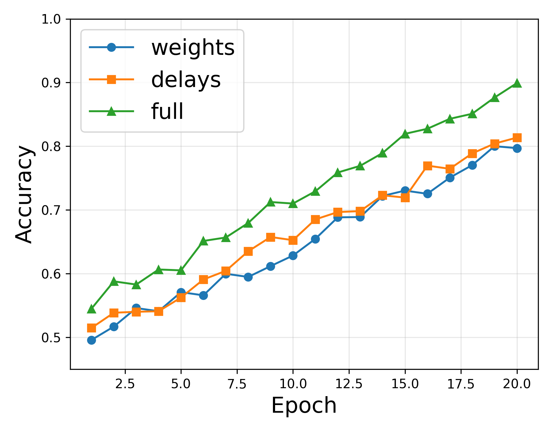
(a) Accuracy

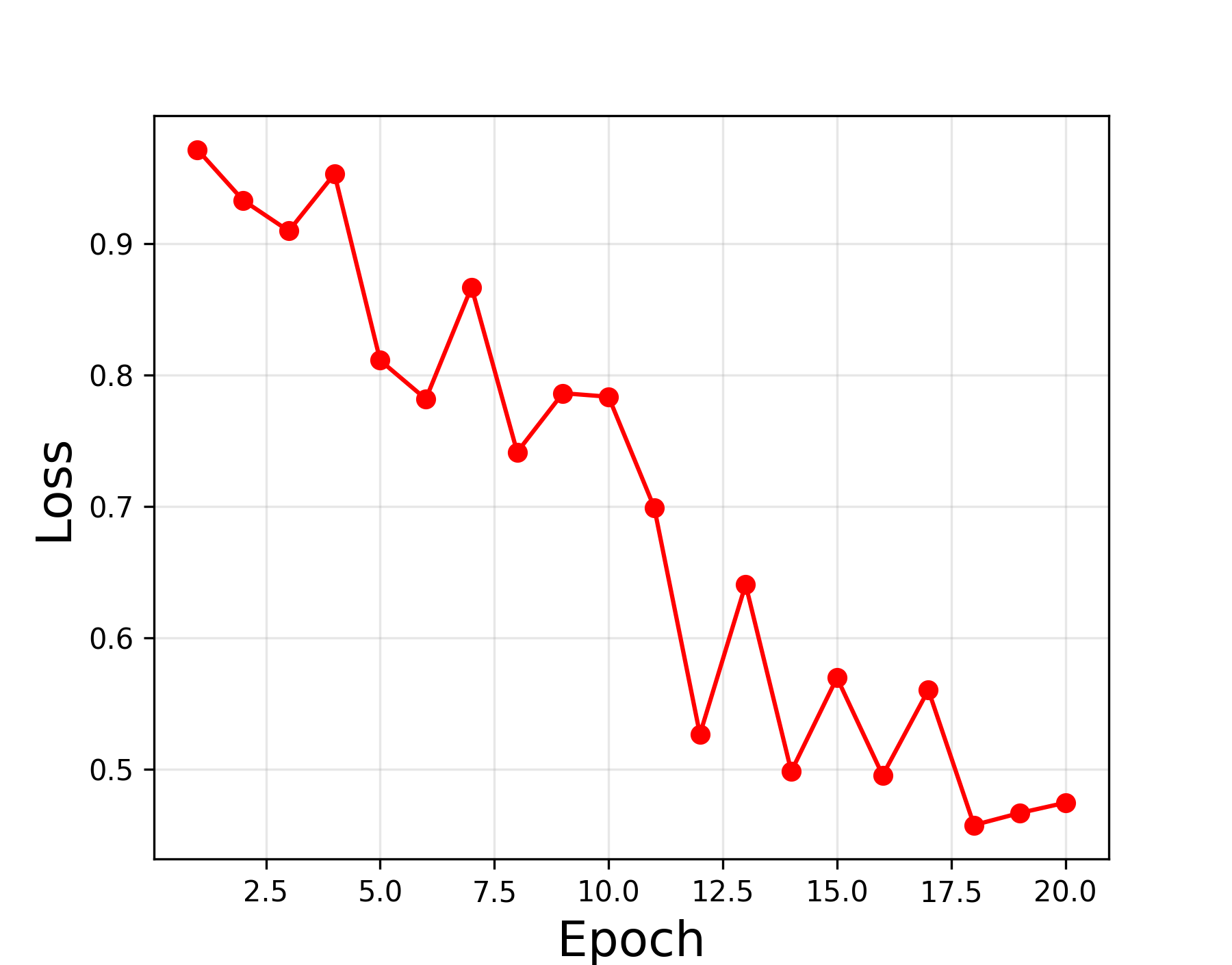
(b) Loss curve

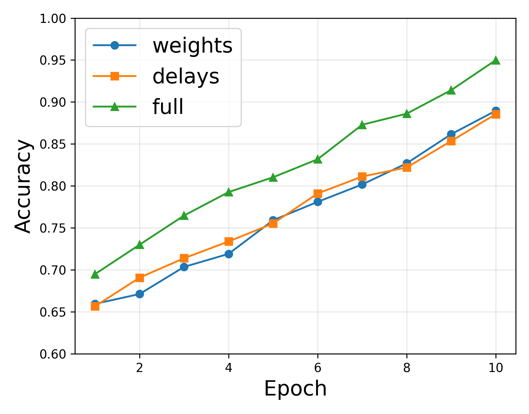
(c) Accuracy

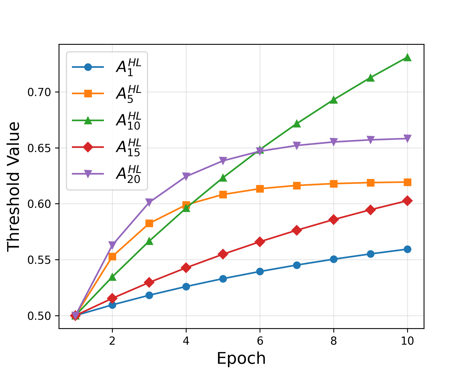
(d) Learned threshold

Figure 3: $(a)$ resp. $(c)$: Accuracy over epochs for the synthetic dataset resp. N-MNIST dataset. $(b)$: Loss curve for the synthetic dataset, revealing that the network learns effectively over multiple epochs. $(d)$: Evolution of the adaptive threshold parameter $A_{j}$ for $5$ out of $20$ hidden layer neurons in the N-MNIST network.

IV-B N-MNIST dataset experiments

To gauge performance on real-world data, we apply the same spiking neural network to a subset of the N-MNIST dataset for the digit classification problem [12, 31]. We select a few classes (e.g., digits 0, 1, and 2) to keep the input dimension manageable for simulation on standard hardware. Each pixel of the image is translated into a spike train using a Poisson process, resulting in a temporal representation of the original static image. We again compare three training modes: weight-only, weight+delay, and full (weights+delays+thresholds).

Fig. 3c displays the evolution of accuracy for these modes across several training epochs. The final accuracy can exceed 90% in some runs, highlighting that the approach remains viable for realistic classification tasks, even though the data is encoded as spikes rather than standard floating-point inputs. In Fig. 3d, we observe a steady decrease in the training loss values. This confirms that the spiking neural network converges to parameters capable of recognizing patterns within the spiking representation of N-MNIST digits.

Fig. 3d, on the other hand, illustrates the evolution of the adaptive threshold parameter $A_{j}$ for five individual neurons in the hidden layer over $10$ training epochs. As shown, all thresholds begin at the initial value of $0.5$ and gradually increase, eventually converging to different values. This behavior indicates that the network selectively reduces neuronal excitability to mitigate extraneous spiking. By adjusting thresholds upward, the model refines its control over firing times, thereby improving classification performance, consistent with the established benefits of moderate spike-frequency adaptation in spatiotemporal pattern recognition.

IV-C Yin-Yang dataset experiments

We conducted a direct comparison using the Yin-Yang dataset as in [27]. Specifically, we trained four variants of our spiking network: $i)$ weights only, $ii)$ weights + delays (results in [27]), $iii)$ weights + thresholds, and $iv)$ full: weights + adaptive thresholds. In this experiment, we used a single hidden layer of $64$ spiking LIF neurons and a $3$-neuron output layer to handle the three-class Yin-Yang problem. We set a learning rate of $0.001$ for all parameters.

Fig. 4 plots the test accuracy across epochs for each variant. Notably, incorporating adaptive thresholds along with training the synaptic delays and weights consistently improved performance, confirming the effectiveness of the proposed approach.

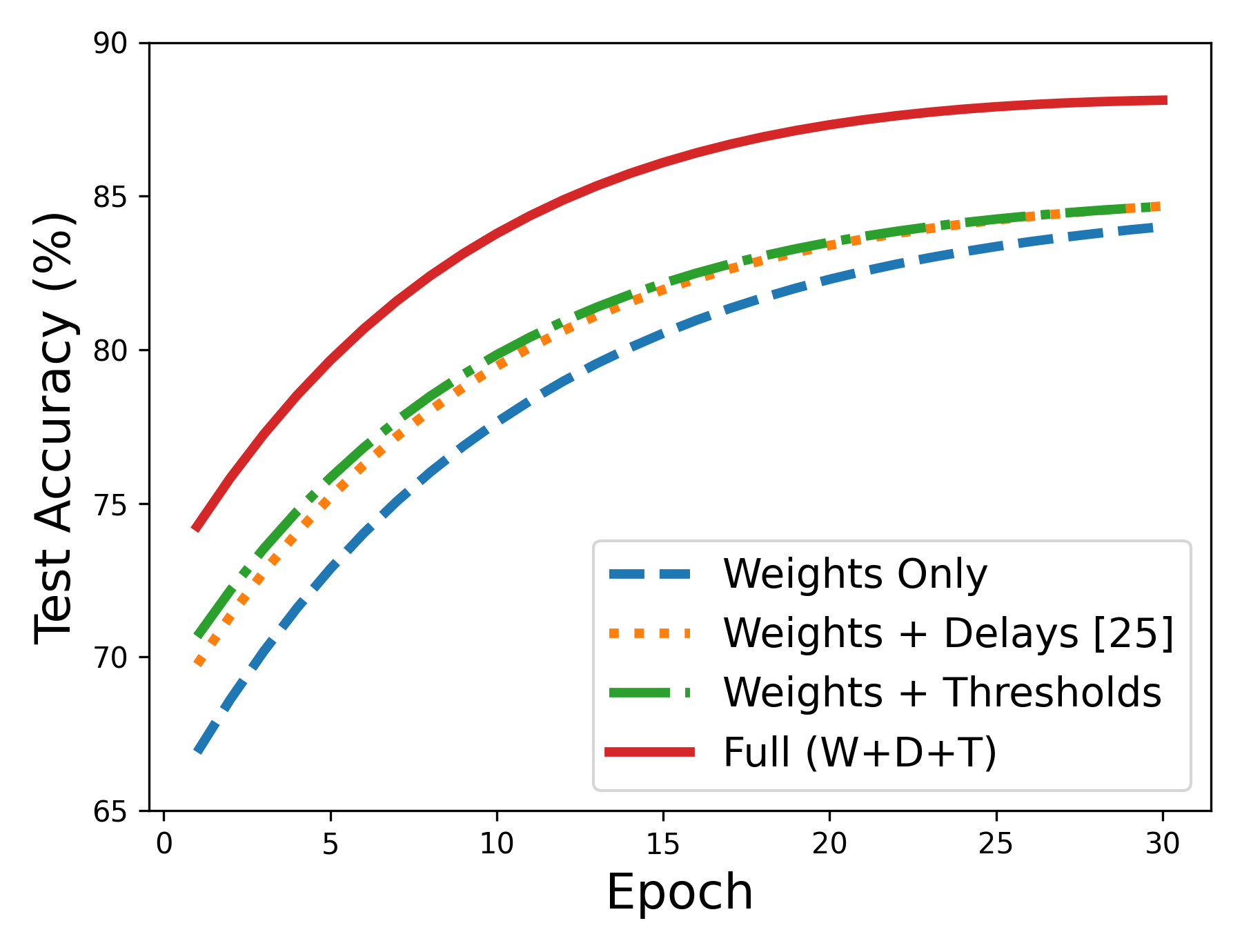
Figure 4: Test accuracy on the Yin-Yang dataset. Our method (weights + delays + adaptive thresholds) achieves the highest final accuracy.

To conclude this section, it is worth noting that whereas our experiments are conducted in software, the proposed framework is inherently aligned with neuromorphic hardware principles. By relying exclusively on spike events and their timing rather than dense membrane traces, the method avoids excessive memory access and continuous updates, thereby paving the way for efficient implementation on event-based platforms like Intel Loihi or BrainScaleS-2. This makes the approach theoretically sound and practically viable for low-power, on-device learning in neuromorphic systems.

V Conclusion

In this work, we have introduced a novel event-driven gradient learning framework for deep spiking neural networks, which co-optimizes synaptic weights, transmission delays, and adaptive neuron thresholds in continuous time. By forgoing discrete-time approximations and surrogate gradients, this approach directly exploited the precise spike timing and naturally incorporated biologically inspired mechanisms such as delayed synaptic transmission and dynamic firing thresholds. Through analytical derivations based on implicit differentiation of spike event timings, we were able to compute exact gradient signals with respect to each of these parameters, thereby expanding the temporal expressiveness and computational power of SNNs. Our experiments confirmed that the co-learning weights, delays, and thresholds significantly enhance accuracy, robustness, and parameter efficiency across multiple benchmarks. By unifying event-driven computation, harnessing spike timing as a valuable resource, biologically inspired threshold adaptation, and exact gradient-based optimization, this work marked an important step toward practical, large-scale neuromorphic systems capable of complex sequence processing and real-time inference.

V-A Future work: Implementation perspective for Loihi

The proposed event-driven learning framework is particularly well-suited for Intel’s Loihi neuromorphic platforms, which support asynchronous spiking and provide ring-buffered synaptic delays and per-synapse weight/delay storage, features that align directly with our algorithm. Building on our software simulations, our ongoing efforts focuses on integrating the framework into the Loihi processor, which can open up a practical and direct pathway for the successful deployment of our approach in hardware implementation.

Beyond this, we believe that this model offers a foundation for precise, event-driven learning in broader neuromorphic hardware applications: it processes only discrete spike events rather than continuous membrane traces, significantly reducing on-chip memory usage and aligning well with hardware constraints such as sparse memory access, temporal locality, and low-power operation.

We, nevertheless, acknowledge that our current assumption, maintaining each neuron’s spike count under small parameter perturbations, may not hold in highly dynamic spiking regimes. In addition, the reliance on exact spike timing presupposes high temporal precision, which may be undermined by hardware noise or quantization effects. A promising path to address the former limitation is to allow controlled transitions in spike counts by applying mild regularity conditions or carefully managing parameter updates when crossing a threshold event. We anticipate that refining these conditions will relax this constraint, an effort we are currently undertaking to make the framework more robust to a wider range of network dynamics.

References

- [1] W. Maass, “Networks of spiking neurons: The third generation of neural network models,” Neural Networks, vol. 10, no. 9, pp. 1659–1671, 1997.
- [2] A. Yousefzadeh, G.-J. Van Schaik, M. Tahghighi, P. Detterer, S. Traferro, M. Hijdra, J. Stuijt, F. Corradi, M. Sifalakis, and M. Konijnenburg, “Seneca: Scalable energy-efficient neuromorphic computer architecture,” in 2022 IEEE 4th International Conference on Artificial Intelligence Circuits and Systems (AICAS). IEEE, 2022, pp. 371–374.
- [3] G. Orchard et al., “Efficient neuromorphic signal processing with loihi 2,” Frontiers in Neuroscience, 2021.
- [4] M. V. Debole et al., “Truenorth: Accelerating from zero to 64 million neurons in 10 years,” Computer, vol. 52, no. 5, pp. 20–29, 2019.
- [5] I. Hammouamri, I. Khalfaoui-Hassani, and T. Masquelier, “Learning delays in spiking neural networks using dilated convolutions with learnable spacings,” arXiv preprint arXiv:2306.17670, 2023.
- [6] M. Yao, G. Zhao, H. Zhang, Y. Hu, L. Deng, Y. Tian, B. Xu, and G. Li, “Attention spiking neural networks,” IEEE transactions on pattern analysis and machine intelligence, vol. 45, no. 8, pp. 9393–9410, 2023.
- [7] Z. Zhou, Y. Zhu, C. He, Y. Wang, S. Yan, Y. Tian, and L. Yuan, “Spikformer: When spiking neural network meets transformer,” arXiv preprint arXiv:2209.15425, 2022.
- [8] S. Deng and S. Gu, “Optimal conversion of conventional artificial neural networks to spiking neural networks,” arXiv preprint arXiv:2103.00476, 2021.
- [9] E. O. Neftci, H. Mostafa, and F. Zenke, “Surrogate gradient learning in spiking neural networks: Bringing the power of gradient-based optimization to spiking neural networks,” IEEE Signal Processing Magazine, vol. 36, no. 6, pp. 51–63, 2019.
- [10] W. Fang, Z. Yu, Y. Chen, T. Huang, T. Masquelier, and Y. Tian, “Deep residual learning in spiking neural networks,” Advances in Neural Information Processing Systems, vol. 34, pp. 21 056–21 069, 2021.
- [11] D. Purves, G. J. Augustine, D. Fitzpatrick, W. Hall, A.-S. LaMantia, and L. White, Neurosciences. De Boeck Supérieur, 2019.
- [12] G. Orchard, A. Jayawant, G. K. Cohen, and N. Thakor, “Converting static image datasets to spiking neuromorphic datasets using saccades,” Frontiers in neuroscience, vol. 9, p. 437, 2015.
- [13] Y. Dan and M.-m. Poo, “Spike timing-dependent plasticity of neural circuits,” Neuron, vol. 44, no. 1, pp. 23–30, 2004.
- [14] W. Maass, “Computing with spiking neurons,” Pulsed neural networks, vol. 2, pp. 55–85, 1999.
- [15] M. Bouvier, A. Valentian, T. Mesquida, F. Rummens, M. Reyboz, E. Vianello, and E. Beigne, “Spiking neural networks hardware implementations and challenges: A survey,” ACM Journal on Emerging Technologies in Computing Systems (JETC), vol. 15, no. 2, pp. 1–35, 2019.
- [16] S. Furber, “Large-scale neuromorphic computing systems,” Journal of neural engineering, vol. 13, no. 5, p. 051001, 2016.
- [17] W. Senn and J.-P. Pfister, “Spike-timing dependent plasticity, learning rules,” in Encyclopedia of Computational Neuroscience. Springer, 2022, pp. 3262–3270.
- [18] A. Taherkhani, A. Belatreche, Y. Li, and L. P. Maguire, “Dl-resume: A delay learning-based remote supervised method for spiking neurons,” IEEE transactions on neural networks and learning systems, vol. 26, no. 12, pp. 3137–3149, 2015.
- [19] S. B. Shrestha and G. Orchard, “Slayer: Spike layer error reassignment in time,” Advances in neural information processing systems, vol. 31, 2018.
- [20] E. Grappolini and A. Subramoney, “Beyond weights: deep learning in spiking neural networks with pure synaptic-delay training,” in Proceedings of the 2023 International Conference on Neuromorphic Systems, 2023, pp. 1–4.
- [21] S. Marom and E. Marder, “A biophysical perspective on the resilience of neuronal excitability across timescales,” Nature Reviews Neuroscience, vol. 24, no. 10, pp. 640–652, 2023.
- [22] J. Benda and R. M. Hennig, “Spike-frequency adaptation generates intensity invariance in a primary auditory interneuron,” Journal of computational neuroscience, vol. 24, pp. 113–136, 2008.
- [23] G. Bellec, D. Salaj, A. Subramoney, R. Legenstein, and W. Maass, “Long short-term memory and learning-to-learn in networks of spiking neurons,” Advances in neural information processing systems, vol. 31, 2018.
- [24] X. Yao, F. Li, Z. Mo, and J. Cheng, “Glif: A unified gated leaky integrate-and-fire neuron for spiking neural networks,” Advances in Neural Information Processing Systems, vol. 35, pp. 32 160–32 171, 2022.
- [25] A. Bittar and P. N. Garner, “Exploring neural oscillations during speech perception via surrogate gradient spiking neural networks,” Frontiers in Neuroscience, vol. 18, p. 1449181, 2024.
- [26] T. C. Wunderlich and C. Pehle, “Event-based backpropagation can compute exact gradients for spiking neural networks,” Scientific Reports, vol. 11, no. 1, p. 12829, 2021.
- [27] J. Göltz, J. Weber, L. Kriener, S. Billaudelle, P. U. Diehl, M. Payvand, and M. A. Petrovici, “Delgrad: Exact event-based gradients in spiking networks for training delays and weights,” arXiv preprint arXiv:2404.19165, 2023.
- [28] D. Auge, J. Hille, E. Mueller, and A. Knoll, “A survey of encoding techniques for signal processing in spiking neural networks,” Neural Processing Letters, vol. 53, no. 6, pp. 4693–4710, 2021.
- [29] W. Gerstner and W. M. Kistler, Spiking neuron models: Single neurons, populations, plasticity. Cambridge university press, 2002.
- [30] S. G. Krantz and H. R. Parks, The implicit function theorem: history, theory, and applications. Springer Science & Business Media, 2002.
- [31] G. Orchard, “N-MNIST: Neuromorphic-MNIST dataset,” https://www.garrickorchard.com/datasets/n-mnist, accessed: 2025-04-09.