The Reconfigurable Earth Observation Satellite Scheduling Problem

Abstract

Earth observation satellites (EOS) play a pivotal role in capturing and analyzing planetary phenomena, ranging from natural disasters to societal development. The EOS scheduling problem (EOSSP), which optimizes the schedule of EOS, is often solved with respect to nadir-directional EOS systems, thus restricting the observation time of targets and, consequently, the effectiveness of each EOS. This paper leverages state-of-the-art constellation reconfigurability to develop the reconfigurable EOS scheduling problem (REOSSP), wherein EOS are assumed to be maneuverable, forming a more optimal constellation configuration at multiple opportunities during a schedule. This paper develops a novel mixed-integer linear programming formulation for the REOSSP to optimally solve the scheduling problem for given parameters. Additionally, since the REOSSP can be computationally expensive for large-scale problems, a rolling horizon procedure (RHP) solution method is developed. The performance of the REOSSP is benchmarked against the EOSSP, which serves as a baseline, through a set of random instances where problem characteristics are varied and a case study in which Hurricane Sandy is used to demonstrate realistic performance. These experiments demonstrate the value of constellation reconfigurability in its application to the EOSSP, yielding solutions that improve performance, while the RHP enhances computational runtime for large-scale REOSSP instances.

Nomenclature

Parameters
$B_{\text{charge}}$  =	Battery gained in one time step of charging
$B_{\text{comm}}$  =	Battery required for one time step of ground station communication
$B_{\text{obs}}$  =	Battery required for one time step of target observation
$B_{\text{time}}$  =	Battery required for one time step of operations
$B_{\text{recon}}$  =	Battery required for one orbital maneuver
$B_{\min}$  =	Minimum battery capacity
$B_{\max}$  =	Maximum battery capacity
$c$  =	Cost of orbital maneuver
$C$  =	Arbitrary weight of data downlink in objective functions
$c_{\max}$  =	Budget for total orbital maneuver costs
$D_{\text{comm}}$  =	Amount of data downlinked per time step
$D_{\text{obs}}$  =	Amount of data from a single observation
$D_{\min}$  =	Minimum data storage capacity
$D_{\max}$  =	Maximum data storage capacity
$G$  =	Number of ground stations
$H$  =	Binary visibility condition of the Sun
$J$  =	Number of orbital slot options
$K$  =	Number of satellites
$L$  =	Number of lookahead stages
$P$  =	Number of targets for observation
$S$  =	Number of reconfiguration stages
$T$  =	Number of time steps
$T_{\text{r}}$  =	Finite schedule duration
$T^{s}$  =	Number of time steps within reconfiguration stages
$V$  =	Binary visibility condition of targets
$W$  =	Binary visibility condition of ground stations
$z_{\text{E}}$  =	EOSSP objective function value
$z_{\text{R}}$  =	REOSSP objective function value
$z^{s}_{\text{RHP}}$  =	RHP objective function value
$Z_{\text{E}}$  =	EOSSP figure of merit
$Z_{\text{R}}$  =	REOSSP figure of merit
$Z_{\text{RHP}}$  =	RHP figure of merit
$\Delta t$  =	Time step size between discrete time steps
Sets
$\mathcal{G}$  =	Set of ground stations
$\mathcal{J}$  =	Set of orbital slot options
$\mathcal{K}$  =	Set of satellites
$\mathcal{P}$  =	Set of targets
$\mathcal{S}$  =	Set of reconfiguration stages
$\mathcal{T}$  =	Set of time steps
$\mathcal{T}^{\ell}$  =	Set of time steps within lookahead stages
$\mathcal{T}^{s}$  =	Set of time steps within reconfiguration stages
Subscripts and indexing
$g$  =	Ground station index
$i,j$  =	Orbital slot option indices
$k$  =	Satellite index
$\ell$  =	Lookahead stage index
$p$  =	Target index
$s$  =	Reconfiguration stage index
$t$  =	Time step index
Decision and indicator variables
$b$  =	Indicator variable of the current battery storage level
$d$  =	Indicator variable of the current data storage level
$h$  =	Decision variable to control solar charging
$q$  =	Decision variable to control data downlink to ground stations
$x$  =	Decision variable to control constellation reconfiguration
$y$  =	Decision variable to control target observation

1 Introduction

Satellite systems are crucial for gathering information on various planetary phenomena on Earth through a practice known as Earth observation (EO), leveraging remote sensing to provide observations in the form of radio frequencies, radar, lidar, and optical imaging, among other measurements. EO data may be used to benefit studies of direct societal activity, such as in use observing agricultural drought progression [1], providing additional security and situational awareness through maritime surveillance [2], and providing insight into current and potential civil infrastructure development [3]. Additionally, EO data may be used to provide necessary information regarding natural processes, such as when utilized to monitor and report on natural disasters [4] and in use modeling the potential spread of diseases [5].

Optimally collecting and providing EO data requires considering the Earth observation satellite scheduling problem (EOSSP), an optimization problem through which each satellite task is treated as a decision variable to maximize observation rewards. Typically, formulations of the EOSSP include the scheduling of observation tasks to gather data, data downlink tasks to transmit data to ground stations, and physical or operational constraints [6, 7, 8]. An important constraint of many EOSSP formulations is the restriction of observation tasks only to times when targets are visible to satellites [9], defined as the visible time window (VTW) [10]. As a result, the amount of data collected through observation is directly influenced by the VTW, further underlining the VTW as one of the most impactful aspects of any EOSSP.

The VTW and the overall amount of data collected are maintained as constant due to underlying assumptions present in many EOSSP formulations. Two such underlying assumptions are the restriction of the pointing direction of satellites, employing only nadir-directional observations which present a fixed VTW, and the restriction to a given orbit that is incapable of being manipulated [11]. Such limitations imply that the VTW is a constant parameter of the EOSSP, thus reducing the potential target observations or data downlink through the restricted VTW access to targets and ground stations (when considered), respectively. The limitations can be alleviated through the use of current state-of-the-art satellite concepts of operations (CONOPS), allowing the VTW to be manipulated as an intermediate decision variable [12].

One such state-of-the-art satellite CONOPS is satellite agility, a key aspect of the agile Earth observation satellite scheduling problem (AEOSSP). Satellite agility refers to the ability of satellites to perform attitude control (slewing) in roll, pitch, and/or yaw [12]. The AEOSSP leverages slewing as an additional task, allowing the satellites to change their pointing angle beyond the nadir direction, thus extending existing VTWs or creating new VTWs that were previously beyond the nadir directional swath width [9]. Prominent formulations of the AEOSSP include the use of slewing to maximize the number or profit of observations under various operational conditions [8, 9, 13, 14] and the use of slewing to prioritize the amount of data returned to a ground station or operator [15, 7, 11]. However, satellite agility suffers from a degradation in observation quality due to the optical tilt and resolution change that results from angled observations, as a large slewing angle causes a difference in the look angle compared to nadir-directional observations [16].

An additional state-of-the-art satellite CONOPS that has not yet been implemented as an extension to the EOSSP is constellation reconfigurability. Constellation reconfigurability is defined as the capability of satellites within a constellation to perform orbital maneuvers to reform the constellation into a more optimal state [17, 18]. Such a capability provides flexibility and responsiveness to satellite systems [19, 20], potentially providing new opportunities for tasks to be performed that were previously unavailable. General uses of constellation reconfigurability external to EO include telecommunications systems with staged satellite deployment for the minimization of overall cost or transfer costs [17, 21], as well as response to incapacitated assets to compensate for performance losses [22]. Investigations of constellation reconfigurability within EO include single-stage reconfiguration for natural disaster impact monitoring [18, 23, 24] and multi-stage reconfiguration for the same purpose [25, 26, 27], reconfiguration between selected operation modes (one selected for regional observation and one for global observation) [19, 28], and altitude changes both for observations of earthquake impacts [29] and tracking mobile targets [30]. Furthermore, previous research in Refs. [31, 32] provides a comparative analysis between nadir-directional, agile, and maneuverable satellites within respective constellations relative to the obtained VTWs by each constellation of 100 historical tropical cyclones. Within the comparative analysis put forth by Ref. [32], the best case of constellation reconfigurability outperforms the nadir-directional and agile satellite constellations by $450.92\text{\,}\%$ and $48.52\text{\,}\%$ on average, respectively, thus depicting promising results regarding the performance of constellation reconfigurability. Each application of constellation reconfigurability has demonstrated beneficial results through performance levels significantly greater than those obtained by fixed constellation configurations. Such research highlights the value that constellation reconfigurability provides to constellation systems, however, each implementation focuses on either maximum observations (maximum VTW), minimum revisit times, or a combination of both, hence neglecting data capacity, battery usage, and data downlink, all of which are key components of the EOSSP.

This paper implements constellation reconfigurability to the EOSSP to develop the Reconfigurable Earth Observation Satellite Scheduling Problem (REOSSP). Constellation reconfigurability is enabled through recent developments in the Multistage Constellation Reconfiguration Problem (MCRP) [25, 26, 27] and is motivated through results indicating the performance level of constellation reconfigurability [31, 32]. The novel REOSSP formulation is developed through the use of mixed-integer linear programming (MILP), enabling the acquisition of provably optimal solutions and the use of commercial optimization problem-solving software. Additionally, the presented formulation incorporates the consideration of onboard data storage, a feature neglected in Refs. [14, 33, 34], as well as onboard battery storage, a feature neglected in Ref. [15], wherein Refs. [8, 12, 10] neglect both features. Inspiration for the inclusion of such rigorous considerations originates from Refs. [6, 7, 35] that consider tasks of target observation, data downlink, and charging, as well as onboard data and battery capacity.

Furthermore, this paper seeks to improve the computation runtime of the REOSSP through the use of a rolling horizon procedure (RHP). RHP is a subset of Model Predictive Control used as an iterative approach to optimize decisions over a given time horizon [36], wherein RHP splits a large problem into multiple smaller subproblems containing a limited portion of the full problem. The use of multiple subproblems reduces the complexity by reducing the size of the solution space within each subproblem. This paper presents the effectiveness of the REOSSP and the computational efficiency enabled through the use of RHP.

In parallel, a novel EOSSP formulation similarly considering onboard data and battery storage over time is developed as a baseline non-reconfigurable equivalent to the REOSSP to benchmark the performance of the REOSSP through experimentation. Such experiments include a set of random instances with varied and randomized parameters, as well as a case study applied to Hurricane Sandy. Through these experiments and the results obtained, the conclusion of Ref. [37] that constellation reconfigurability greatly outperforms a standard nadir-directional constellation without reconfigurability is reinforced. Therefore, this paper additionally serves as further proof of concept for implementation constellation reconfigurability to the EOSSP at a higher level of fidelity and operational complexity than previous research.

An illustrative example of the capabilities of the REOSSP for a constellation of two satellites is shown in Fig. 1, including a representation of all tasks and operational constraints. Tasks, such as orbital maneuvering, target observation, data downlink to a ground station, and charging, are shown through arrows in the direction of the task, while the state of variables relating to operational constraints, such as the battery, data, and fuel capacities, are shown as a form of level that represents the current capacity. The initial state of the constellation is at $t_{0}$, where both satellites have no visibility of a given target. As a result of no present visibility, both satellites perform orbital maneuvers to form a more optimal configuration, a process that drains both the onboard battery and fuel. The reconfigured state of the constellation is at $t_{1}$, which has now gained visibility of the target, thus observing the target and contributing to the onboard data storage while further draining the onboard battery. At $t_{2}$, an observation of the target has been completed and may not be required to be performed again, leading both satellites to replenish the onboard battery storage through solar charging. Additionally, one satellite in this portion will not have visibility of the ground station, and as such this satellite performs an additional orbital maneuver to gain said visibility. Finally, $t_{3}$ shows the final state of the constellation with both satellites downlinking the observed data to the ground station, transmitting the data currently stored at the cost of more battery power. Furthermore, this portion shows the additional drain on the fuel of the satellite that performed an additional orbital maneuver.

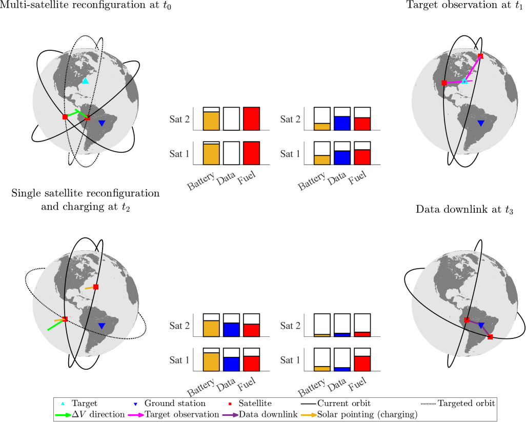
Figure 1: A demonstration of the capabilities enabled in the REOSSP.

The rest of this paper is organized as follows. Sections 2 and 3 introduce slightly modified versions of the MILP formulations of the EOSSP and REOSSP, respectively. Then, Sec. 4 introduces an algorithmic solution method to the REOSSP using RHP, a novel formulation referred to as the RHP. Next, Sec. 5 conducts a thorough comparative analysis between the EOSSP, REOSSP, and RHP, including instances with randomized parameters and a real-world case study using historical data from Hurricane Sandy. Finally, Sec. 6 provides a review of overall results and contributes several possible directions for future research.

2 Earth Observation Satellite Scheduling Problem - Baseline

To incorporate constellation reconfigurability into the EOSSP, a baseline formulation is developed in such a way as to be expanded for the reconfiguration process, which also proves useful as a comparison between a reconfigurable and a non-reconfigurable solution. This formulation is henceforth denoted as the EOSSP. The formulation of the EOSSP in this paper is an optimization problem making use of MILP to schedule tasks of target observation, data downlink to ground stations, and solar panel charging. Each task is constrained by physical capabilities, data storage availability, and/or battery power availability.

The overall finite schedule duration is designated as $T_{\text{r}}$, which is discretized by a time step size $\Delta t>0$ to result in the finite number of discrete time steps $T=T_{\text{r}}/\Delta t$. The set of time steps, defined as $\mathcal{T}=\{1,2,\ldots,T\}$, contains all time steps at which a task can be performed. There also exists a set of satellites $\mathcal{K}=\{1,2,\ldots,K\}$ containing $K$ total satellites and the associated classical orbital elements, a set of targets for observation and associated positions defined as $\mathcal{P}=\{1,2,\ldots,P\}$ where $P$ is the total number of targets, and a set of ground stations for the downlink of data and associated positions defined as $\mathcal{G}=\{1,2,\ldots,G\}$ where $G$ is the total number of ground stations.

The EOSSP also utilizes various parameters within the problem constraints. The visibility of target $p\in\mathcal{P}$ by satellite $k\in\mathcal{K}$ at time step $t\in\mathcal{T}$ is contained in $V^{k}_{tp}$ as a binary value dependent on if $p$ is visible (one) or not (zero). Similarly, the visibility of ground station $g\in\mathcal{G}$ by satellite $k$ at time step $t$ is contained in $W^{k}_{tg}$ also as a binary value dependent on if $g$ is visible (one) or not (zero). Lastly, the visibility of the Sun by satellite $k$ at time step $t$ is contained in $H^{k}_{t}$ as a binary value.

Finally, the data and battery storage levels are tracked for each satellite $k$ from each time step $t$ to the next $t+1$. The current data storage level is determined by tracking the data gained through target observations and the data transmitted through downlink to any ground station. Additionally, the data storage level of each satellite $k$ is restricted to not deplete below a minimum threshold $D^{k}_{\min}$ and not accumulate more than the data storage capacity of the satellite, defined as $D^{k}_{\max}$. Similarly, the current battery storage level is determined by tracking the energy drained by observation, data downlink, and standard operational tasks such as tracking telemetry and time, and the energy replenished by charging through sunlight exposure. The battery storage level of each satellite $k$ is also restricted to not deplete below a minimum threshold $B^{k}_{\min}$ and not accumulate more than the battery capacity, defined as $B^{k}_{\max}$.

2.1 Decision Variables and Indicator Variables

The decision variables of the EOSSP are the tasks being scheduled throughout the duration of a given schedule, with additional indicator variables that track the data storage and battery levels over time. Each decision variable task is defined as binary such that a value of one corresponds to the task being performed and a value of zero corresponds to the task not being performed, while the indicator variables are defined as real numbers with upper and lower bounds defined as the maximum and minimum storage capacities (zero), respectively. Each of these variables is applied to each satellite $k$ and time step $t$ in the overall schedule horizon, while the tasks additionally apply to their associated objective.

The first decision variable is the observation of target $p$ as performed by satellite $k$ at time $t$:

$$y^{k}_{tp}\in\{0,1\},\quad t\in\mathcal{T},p\in\mathcal{P},k\in\mathcal{K}$$ (1)

The second decision variable is the downlink of data to ground station $g$ as performed by satellite $k$ at time $t$:

$$q^{k}_{tg}\in\{0,1\},\quad t\in\mathcal{T},g\in\mathcal{G},k\in\mathcal{K}$$ (2)

The third decision variable is the solar charging of satellite $k$ at time $t$:

$$h^{k}_{t}\in\{0,1\},\quad t\in\mathcal{T},k\in\mathcal{K}$$ (3)

The first indicator variable tracks the current data storage level of satellite $k$ at time $t$ and is defined with a minimum of $D^{k}_{\min}$ and a maximum of $D^{k}_{\max}$:

$$d^{k}_{t}\in[D^{k}_{\min},D^{k}_{\max}],\quad t\in\mathcal{T},k\in\mathcal{K}$$ (4)

The second indicator variable similarly tracks the current battery storage level of satellite $k$ at time $t$ and is defined with a minimum of $B^{k}_{\min}$ and a maximum of $B^{k}_{\max}$:

$$b^{k}_{t}\in[B^{k}_{\min},B^{k}_{\max}],\quad t\in\mathcal{T},k\in\mathcal{K}$$ (5)

2.2 Objective Function

The objective of the EOSSP balances the observation and subsequent downlink of data to ground stations, more heavily prioritizing the downlink of data through an arbitrary weight, $C>1$. The objective function value of the EOSSP is denoted as $z_{\text{E}}$ obtained via:

$$z_{\text{E}}=\sum_{k\in\mathcal{K}}\sum_{t\in\mathcal{T}}\left(\sum_{g\in\mathcal{G}}Cq^{k}_{tg}+\sum_{p\in\mathcal{P}}y^{k}_{tp}\right)$$ (6)

where $z_{\text{E}}$ is determined through the weighted number of downlink tasks performed by the decision variable $q^{k}_{tg}$ and the unweighted number of observation tasks performed by the decision variable $y^{k}_{tp}$ with respect to all $K$ satellites, all $T$ time steps, and all $G$ ground stations or all $P$ targets for decision variables $q^{k}_{tg}$ and $y^{k}_{tp}$, respectively. Alternatively, the figure of merit for the EOSSP corresponds to the amount of data downlinked to ground stations, obtained via:

$$Z_{\text{E}}=\sum_{k\in\mathcal{K}}\sum_{t\in\mathcal{T}}\sum_{g\in\mathcal{G}}D_{\text{comm}}q^{k}_{tg}$$ (7)

where $D_{\text{comm}}$ is the amount of transmitted during a single time step. The objective function value, $z_{\text{E}}$, and the figure of merit, $Z_{\text{E}}$, are both used to compare the performance of the EOSSP to the REOSSP and RHP.

2.3 Constraints

The EOSSP contains constraints, including the application of target visibility, ground station visibility, Sun visibility, maximum (and minimum) data storage capacity, and maximum (and minimum) battery storage capacity.

2.3.1 Time Window Constraints

Each task is restricted to only be performed when visibility of the associated task is available to each satellite individually; these constraints define the VTW for each task utilizing the associated parameter for visibility such as $V^{k}_{tp}$ for targets observation, $W^{k}_{tg}$ for ground station downlink, and $H^{k}_{t}$ for solar panel charging, respectively. Additionally, power-related tasks such as target observation, data downlink, and solar charging are restricted to occurring exclusively from one another.

$$V^{k}_{tp}\geq y^{k}_{tp},\quad \forall t\in\mathcal{T},\forall p\in\mathcal{P},\forall k\in\mathcal{K}$$ (8a)

$$W^{k}_{tg}\geq q^{k}_{tg},\quad \forall t\in\mathcal{T},\forall g\in\mathcal{G},\forall k\in\mathcal{K}$$ (8b)

$$H^{k}_{t}\geq h^{k}_{t},\quad \forall t\in\mathcal{T},\forall k\in\mathcal{K}$$ (8c)

$$\sum_{p\in\mathcal{P}}y^{k}_{tp}+\sum_{g\in\mathcal{G}}q^{k}_{tg}+h^{k}_{t}\leq 1,\quad \forall t\in\mathcal{T},\forall k\in\mathcal{K}$$ (8d)

Constraints (8a), (8b), and (8c) restrict the observation of targets, downlink of data to ground stations, and solar charging to the associated VTW, respectively. These constraints operate under the assumption that only one satellite is required to perform each task such that each satellite operates independently. Additionally, constraints (8d) restrict observations, data downlink, and solar charging only to be performed in exclusion to one another, ensuring that each satellite must choose which task to perform if the VTW of each task overlaps. Such a consideration is in place for battery routing consideration to not overload the simultaneous power exchange within an onboard batter, similar to the task overlap exclusion employed in Ref. [38]. Additionally, these constraints ensure that only one target may be viewed at each time step or that only one ground station may be utilized for data downlink for the same reason.

A demonstration of the visibility conditions in constraints (8a), (8b), and (8c) as well as the overlap exclusion conditions in constraints (8d) is shown in Fig. 2. Within the figure, illustrative binary visibility parameters $V^{k}_{tp}$, $W^{k}_{tp}$, and $H^{k}_{t}$ are shown through blue, red, and orange boxes, respectively, indicating time along a horizon with visibility of the associated goal, and the binary decision variables $y^{k}_{tp}$, $q^{k}_{tg}$, and $h^{k}_{t}$ are shown similarly. The figure depicts some key occurrences resulting from the above constraints, labeled as time steps $t_{1}$ through $t_{5}$. First, time step $t_{1}$ depicts the visibility of a ground station with no downlink occurrence as a result of no prior observations contributing data to be downlinked. Next time step $t_{2}$ depicts the visibility of the Sun along with the subsequent solar charging. Then, time step $t_{3}$ shows the visibility and subsequent observation of a target, and time step $t_{4}$ illustrates the visibility of a ground station that allows the downlink of the previously observed data. Finally, time step $t_{5}$ depicts the enforcement of constraints (8d), restricting only one task to occur at each time step, despite all three tasks having visibility of the associated goal at various times. The enforcement of constraints (8d) additionally applies to the simultaneous visibility of different targets and ground stations, though this is not shown in the figure directly.

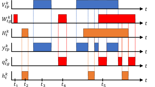
Figure 2: Feasible observation, downlink, and solar charging occurrence.

2.3.2 Data Tracking and Storage Constraints

The second set of constraints tracks the usage of each satellite’s onboard data storage, determining when data is gained or downlinked and restricting the data so that it does not overflow the onboard storage limit or deplete below zero data in storage.

$$d^{k}_{t+1}=d^{k}_{t}+\sum_{p\in\mathcal{P}}D_{\text{obs}}y^{k}_{tp}-\sum_{g\in\mathcal{G}}D_{\text{comm}}q^{k}_{tg},\quad \forall t\in\mathcal{T}\setminus\{T\},\forall k\in\mathcal{K}$$ (9a)

$$d^{k}_{t}+\sum_{p\in\mathcal{P}}D_{\text{obs}}y^{k}_{tp}\leq D^{k}_{\max},\quad \forall t\in\mathcal{T},\forall k\in\mathcal{K}$$ (9b)

$$d^{k}_{t}-\sum_{g\in\mathcal{G}}D_{\text{comm}}q^{k}_{tg}\geq D^{k}_{\min},\quad \forall t\in\mathcal{T},\forall k\in\mathcal{K}$$ (9c)

Constraints (9a) track the data storage of each satellite at each time step, ensuring that the tasks performed at time step $t$ contribute to the data storage level at time step $t+1$, where $D_{\text{obs}}\geq 0$ is the amount of data acquired through one observation and $D_{\text{comm}}\geq 0$ is the amount of data able to be downlinked to a ground station within one time step. Furthermore, $D_{\text{obs}}$ is a constant value of given units while $D_{\text{comm}}$ is obtained by multiplying a data transmission rate in units/time by $\Delta t$ (in the same units of time) to obtain a discrete constant value. It is also assumed that each satellite begins with the minimum data storage value such that $d^{k}_{1}=D^{k}_{\min},~\forall k\in\mathcal{K}$, allowing the first data observed to contribute at time $t=1$ for the data storage level of $d^{k}_{2}$. Constraints (9b) ensure that the data stored within each satellite through observation does not exceed the maximum capacity set by $D^{k}_{\max}$. Similarly, constraints (9c) ensure that the data transmitted to a ground station does not exceed the actual amount of data contained by the satellite.

A demonstration of the control and contribution of the data storage for each satellite is shown in Fig. 3, with similar key occurrences denoted by time steps $t_{1}$ through $t_{5}$. First, time steps $t_{1}$ and $t_{2}$ depict the contribution of observations and the drain of downlink to the onboard data storage, respectively, provided through constraints (9a). Then, time steps $t_{3}$ and $t_{4}$ depict the halt of observations such that the onboard data level does not exceed the maximum capacity set by $D^{k}_{\max}$, provided through constraints (9b). Finally, time step $t_{5}$ depicts the halt of downlink once the data level is fully drained, ensuring the current data level remains non-negative, provided through constraints (9c).

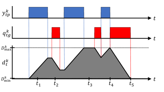
Figure 3: Visualization of the data storage level of satellite $k$.

2.3.3 Battery Tracking and Storage Constraints

The third and final set of constraints tracks the usage of the onboard battery power of each satellite, similarly to that of the data tracking constraints, determining when the battery is charged or depleted as well as restricting the power to not overflow onboard battery limits and not deplete below the minimum capacity.

$$b^{k}_{t+1}=b^{k}_{t}+B_{\text{charge}}h^{k}_{t}-\sum_{p\in\mathcal{P}}B_{\text{obs}}y^{k}_{tp}-\sum_{g\in\mathcal{G}}B_{\text{comm}}q^{k}_{tg}-B_{\text{time}},\quad \forall t\in\mathcal{T}\setminus\{T\},\forall k\in\mathcal{K}$$ (10a)

$$b^{k}_{t}+B_{\text{charge}}h^{k}_{t}\leq B^{k}_{\max},\quad \forall t\in\mathcal{T},\forall k\in\mathcal{K}$$ (10b)

$$b^{k}_{t}-\sum_{p\in\mathcal{P}}B_{\text{obs}}y^{k}_{tp}-\sum_{g\in\mathcal{G}}B_{\text{comm}}q^{k}_{tg}-B_{\text{time}}\geq B^{k}_{\min},\quad \forall t\in\mathcal{T},\forall k\in\mathcal{K}$$ (10c)

Constraints (10a) track the battery level of each satellite at each time step, where $B_{\text{charge}}\geq 0$ is the amount of power able to be charged, $B_{\text{obs}}\geq 0$ is the amount of power required for observation to occur, $B_{\text{comm}}\geq 0$ is the amount of power required for a data downlink transmission, and $B_{\text{time}}\geq 0$ is the power required for normal operational tasks such as telemetry and timekeeping. Each power value accounts for one time step and is found by multiplying a charge rate in units/time by $\Delta t$ to obtain a power value in the given units. It is similarly assumed that each satellite begins with a full battery charge such that $b^{k}_{1}=B^{k}_{\max},~\forall k\in\mathcal{K}$, allowing the first power draw occurring at $t=1$ to contribute to the battery storage level of $b^{k}_{2}$. Constraints (10b) ensure that the power contained within each satellite through charging does not exceed the maximum capacity of the battery set by $B^{k}_{\max}$. Similarly, constraints (10c) ensure that the power required by other task performance does not drain the battery below the minimum capacity set by $B^{k}_{\min}$.

Figure 4 visualizes the battery consumption similarly to Fig. 3, with key occurrences denoted by time steps $t_{1}$ through $t_{4}$. First, time step $t_{1}$ demonstrates the constant battery drain caused by normal operational tasks, $B_{\text{time}}$, and time step $t_{2}$ demonstrates the combined battery drain of the constant drain and observation. Then, time step $t_{3}$ demonstrates the battery charging as a result of charging operations while within Sun visibility. Finally, time step $t_{4}$ reiterates the task overlap exclusion from constraints (8d). Such consumption of battery power additionally applies to data downlink, though not shown directly in the figure.

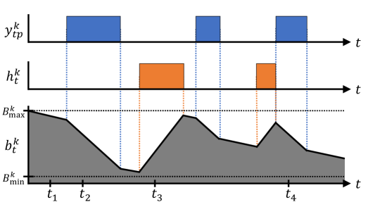
Figure 4: Visualization of the battery level of satellite $k$.

2.4 Full Formulation

Given the objective function, constraints, decision variables, and indicator variables, the full EOSSP is defined as follows:

$$\begin{split}\max&\quad z_{\text{E}}\\ \text{s.t.}&\quad\text{Constraints \eqref{EOSSP:y}-\eqref{EOSSP:obj}, \eqref{EOSSP:Visibility}-\eqref{EOSSP:Battery}}\end{split}$$ (EOSSP)

The objective function balances the number of occurrences of data downlink to any ground stations $g\in\mathcal{G}$ with the less heavily weighted number of occurrences of the observation of any targets $p\in\mathcal{P}$, while the constraints restrict the problem to the observation of data prior to data downlink, the assurance of available data storage, and the assurance of available power for task completion. Additionally, the EOSSP provides the schedule of charging, observation, and data downlink performed by a constellation of satellites over a given time horizon.

3 Reconfigurable Earth Observation Satellite Scheduling Problem

The REOSSP formulation, henceforth referred to as the REOSSP, is an extension of the EOSSP that incorporates satellite maneuvering tasks in addition to the tasks present in the EOSSP, thus allowing a new degree of freedom through orbital maneuvers. The constellation reconfiguration process is derived from the MCRP, obtained from Refs. [25, 26, 27].

The overall schedule duration and discrete time interval remain as $T_{\text{r}}$, $\Delta t>0$, and $T=T_{\text{r}}/\Delta t$ as well as $\mathcal{T}=\{1,2,\ldots,T\}$. Additionally, within $\mathcal{T}$ there exists a set of equally spaced stages at which each satellite in the constellation can perform orbital maneuvers, defined as $\mathcal{S}=\{0,1,2,\ldots,S\}$, where $S$ is the number of equally spaced stages and stage $s=0$ is the stage wherein the initial configuration of the constellation is present. As a result of each stage being equally spaced in $\mathcal{T}$, there exists a set of time steps within each stage defined as $\mathcal{T}^{s}=\{1,2,\ldots,T^{s}\}$ where $T^{s}=T/S$ is an integer defining the number of time steps per stage. Alongside the addition of stages, each satellite within the set of satellites $\mathcal{K}$ (consistent with the EOSSP) contains an associated set of orbital slots allotted for each stage as transfer (orbital maneuver) options. The orbital slots are defined as $\mathcal{J}^{sk}=\{1,2,\ldots,J^{sk}\}$ where $J^{sk}$ is the total number of available slots for satellite $k\in\mathcal{K}$ and stage $s\in\mathcal{S}$.

The REOSSP also expands upon the parameters given in the EOSSP. The most important extension is the addition of two dimensions to the visibility of targets, ground stations, and the Sun, allowing the current stage and the currently occupied orbital slot of each satellite to be accounted for. Through this extension, the visibility of each target $p\in\mathcal{P}$ is now defined relative to the satellite $k$, stage $s\in\mathcal{S}\setminus\{0\}$, orbital slot $j\in\mathcal{J}^{sk}$, and time $t\in\mathcal{T}^{s}$ in $V^{sk}_{tjp}$ as a binary value. The visibility of ground stations and the Sun follows in the same manner in $W^{sk}_{tjg}$ and $H^{sk}_{tj}$ as binary values, respectively. Additionally, the cost of transfer between two orbital slots of a given satellite and a given stage is $c^{sk}_{ij}$, defined as the transfer between slot $i\in\mathcal{J}^{s-1,k}$ in the previous stage configuration ($s-1$) to slot $j\in\mathcal{J}^{sk}$ in the current stage ($s$) relative to satellite $k$ and stage $s\in\mathcal{S}\setminus\{0\}$. Furthermore, the maximum transfer cost for the entire schedule is allotted to each satellite as $c^{k}_{\max},~\forall k\in\mathcal{K}$. Finally, battery power and data storage are tracked in a similar manner with the same upper bounds.

3.1 Decision Variables

The decision variables and indicator variables of the REOSSP are the same tasks and indicators included in the EOSSP, with additional dimensionality regarding reconfiguration stages and an additional task to control the maneuvers of each satellite.

The first decision variable is the path of orbital maneuvers, defined as the sequence of maneuvers of satellite $k$ from an orbital slot $i\in\mathcal{J}^{s-1,k}$ in the previous stage to an orbital slot $j\in\mathcal{J}^{sk}$ in the current stage for all stages $s\in\mathcal{S}\setminus\{0\}$ such that the initial condition, $\mathcal{J}^{0k}$ is transferred from at stage $s=1$:

$$x^{sk}_{ij}\in\{0,1\},\quad s\in\mathcal{S}\setminus\{0\},k\in\mathcal{K},i\in\mathcal{J}^{s-1,k},j\in\mathcal{J}^{sk}$$ (11)

It should be noted that $\mathcal{J}^{0k}$ is a singleton set representing the initial orbital slot in which satellite $k$ is located. The second decision variable is the observation of target $p$ as performed by satellite $k$ during stage $s\in\mathcal{S}\setminus\{0\}$ at time $t$:

$$y^{sk}_{tp}\in\{0,1\},\quad s\in\mathcal{S}\setminus\{0\},t\in\mathcal{T}^{s},p\in\mathcal{P},k\in\mathcal{K}$$ (12)

The third decision variable is the downlink of data to ground station $g$ as performed by satellite $k$ during stage $s\in\mathcal{S}\setminus\{0\}$ at time $t$:

$$q^{sk}_{tg}\in\{0,1\},\quad s\in\mathcal{S}\setminus\{0\},t\in\mathcal{T}^{s},g\in\mathcal{G},k\in\mathcal{K}$$ (13)

The final binary decision variable is the charging of satellite $k$ during stage $s\in\mathcal{S}\setminus\{0\}$ at time $t$:

$$h^{sk}_{t}\in\{0,1\},\quad s\in\mathcal{S}\setminus\{0\},t\in\mathcal{T}^{s},k\in\mathcal{K}$$ (14)

The first indicator variable is used to track the data storage capacity of each satellite over the entire discrete schedule horizon, concerning the discrete stages, represented as the data storage level of satellite $k$ during stage $s\in\mathcal{S}\setminus\{0\}$ at time $t$:

$$d^{sk}_{t}\in[D^{k}_{\min},D^{k}_{\max}],\quad s\in\mathcal{S}\setminus\{0\},t\in\mathcal{T}^{s},k\in\mathcal{K}$$ (15)

The second indicator variable is used to track the battery capacity of each satellite over the entire discrete schedule horizon, concerning the discrete stages, represented as the battery level of satellite $k$ during stage $s\in\mathcal{S}\setminus\{0\}$ at time $t$:

$$b^{sk}_{t}\in[B^{k}_{\min},B^{k}_{\max}],\quad s\in\mathcal{S}\setminus\{0\},t\in\mathcal{T}^{s},k\in\mathcal{K}$$ (16)

3.2 Objective Function

The objective function of the REOSSP mirrors the EOSSP, balancing the observation and subsequent downlink of data to ground stations with the same weighting $C$ to prioritize the downlink of data. The objective function value of the REOSSP is denoted as $z_{\text{R}}$ obtained via:

$$z_{\text{R}}=\sum_{k\in\mathcal{K}}\sum_{s\in\mathcal{S}\setminus\{0\}}\sum_{t\in\mathcal{T}^{s}}\left(\sum_{g\in\mathcal{G}}Cq^{sk}_{tg}+\sum_{p\in\mathcal{P}}y^{sk}_{tp}\right)$$ (17)

where $z_{\text{R}}$ is determined through the weighted number of downlink tasks performed by the decision variable $q^{sk}_{tg}$ and the unweighted number of observation tasks performed by the decision variable $y^{sk}_{tp}$ with respect to all $K$ satellites, all $S$ reconfiguration stages, all $T^{s}$ time steps per reconfiguration stage, and all $G$ ground stations or all $P$ targets for decision variables $q^{sk}_{tg}$ and $y^{sk}_{tp}$, respectively. Similarly to the EOSSP, the figure of merit for the REOSSP corresponds to the amount of data downlinked to ground stations, obtained via:

$$Z_{\text{R}}=\sum_{k\in\mathcal{K}}\sum_{s\in\mathcal{S}\setminus\{0\}}\sum_{t\in\mathcal{T}^{s}}\sum_{g\in\mathcal{G}}D_{\text{comm}}q^{sk}_{tg}$$ (18)

The objective function value, $z_{\text{R}}$, and the figure of merit, $Z_{\text{R}}$, are used to compare the performance of the REOSSP to the EOSSP and RHP. To distinguish the resultant objective function values and figure of merit values, the subscript R is used in place of the subscript E.

3.3 Constraints

The REOSSP contains similar constraints to the EOSSP, but with extended dimensionality to incorporate stages and reflect the effects of the reconfiguration process through new satellite positioning and resources required to perform such maneuvers.

3.3.1 Orbital Maneuver Path Continuity Constraints

The first set of constraints restricts the path of constellation reconfigurability to feasible maneuvering sequences concerning a given budget for propellant.

$$\sum_{j\in\mathcal{J}^{1k}}x^{1k}_{ij}=1,\quad \forall k\in\mathcal{K},\forall i\in\mathcal{J}^{0k}$$ (19a)

$$\sum_{j\in\mathcal{J}^{s+1,k}}x^{s+1,k}_{ij}-\sum_{j^{\prime}\in\mathcal{J}^{s-1,k}}x^{sk}_{j^{\prime}i}=0,\quad \forall s\in\mathcal{S}\setminus\{0,S\},\forall k\in\mathcal{K},\forall i\in\mathcal{J}^{sk}$$ (19b)

$$\sum_{s\in\mathcal{S}\setminus\{0\}}\sum_{i\in\mathcal{J}^{s-1,k}}\sum_{j\in\mathcal{J}^{sk}}c^{sk}_{ij}x^{sk}_{ij}\leq c^{k}_{\max},\quad \forall k\in\mathcal{K}$$ (19c)

Constraints (19a) ensure that only one orbital slot in the first stage ($\mathcal{J}^{1k}$) can be selected for transfer from the initial condition ($\mathcal{J}^{0k}$), ensuring that one satellite cannot occupy multiple positions at one time. Constraints (19b) similarly ensure that only one orbital slot in subsequent stages is selected for transfer, but also extends the condition to state that the satellite can only transfer from the current slot ($i\in\mathcal{J}^{sk}$) if it arrived there previously. Both constraints ensure that satellites do not conduct transfers from positions in which they may not be located. Finally, constraints (19c) restrict the allowable transfer between slots to within the maximum propellant budget of the satellite.

A demonstration of feasible path continuity and maneuvering is shown in Fig. 5, depicting the possible paths taken by any number of satellites for any number of orbital slots or stages where the highlighted paths represent $x^{sk}_{ij}=1$. The figure notes that the initial condition and first orbital maneuvers occur outside of the time horizon such that the constellation configuration at stage $s=1$ is formed at time $t=1$ and subsequent stages occur at the corresponding $t=1+(s-1)T^{s}$ time. Additionally, the figure demonstrates the option to remain within the current orbital slot, such as satellite $K$ in stage two, resulting in a cost $c^{sk}_{ij}$ of zero.

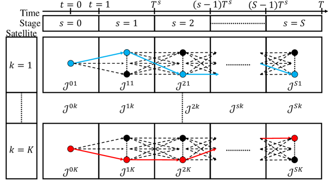
Figure 5: Feasible orbital maneuver progression for $K$ satellites.

3.3.2 Time Window Constraints

The second set of constraints restricts target observation, data downlink to ground stations, and solar charging to the available VTWs, as well as enforcing the task overlap exclusion of each task. These constraints account for the orbital maneuver path and subsequent satellite orbital slot positions within each reconfiguration stage.

$$\sum_{i\in\mathcal{J}^{s-1,k}}\sum_{j\in\mathcal{J}^{sk}}V^{sk}_{tjp}x^{sk}_{ij}\geq y^{sk}_{tp},\quad \forall s\in\mathcal{S}\setminus\{0\},\forall t\in\mathcal{T}^{s},\forall p\in\mathcal{P},\forall k\in\mathcal{K}$$ (20a)

$$\sum_{i\in\mathcal{J}^{s-1,k}}\sum_{j\in\mathcal{J}^{sk}}W^{sk}_{tjg}x^{sk}_{ij}\geq q^{sk}_{tg},\quad \forall s\in\mathcal{S}\setminus\{0\},\forall t\in\mathcal{T}^{s},\forall g\in\mathcal{G},\forall k\in\mathcal{K}$$ (20b)

$$\sum_{i\in\mathcal{J}^{s-1,k}}\sum_{j\in\mathcal{J}^{sk}}H^{sk}_{tj}x^{sk}_{ij}\geq h^{sk}_{t},\quad \forall s\in\mathcal{S}\setminus\{0\},\forall t\in\mathcal{T}^{s},\forall k\in\mathcal{K}$$ (20c)

$$\sum_{p\in\mathcal{P}}y^{sk}_{tp}+\sum_{g\in\mathcal{G}}q^{sk}_{tg}+h^{sk}_{t}\leq 1,\quad \forall s\in\mathcal{S}\setminus\{0\},\forall t\in\mathcal{T}^{s},\forall k\in\mathcal{K}$$ (20d)

Constraints (20a), (20b), and (20c) restrict target observation, data downlink, and solar charging to the associated VTW, respectively, dependent upon the current orbital slot occupied. The orbital maneuver flow allows the attainment of a new visibility profile in either $V^{sk}_{tjp},~W^{sk}_{tjg}$, or $H^{sk}_{tj}$, creating a new VTW of the target, ground station, or the Sun, which is then defined as the only time that the tasks are allowed to be performed. These constraints operate under the assumption that only one satellite is required for task performance, ensuring independent operation. Constraints (20d) restrict each task to only be performed exclusively of other tasks, additionally ensuring that only one target or ground station may be selected for observation or data downlink, respectively, at each time step.

3.3.3 Data Tracking and Storage Constraints

The third set of constraints tracks the usage of the onboard data storage level of each satellite, determining when data is gained or downlinked as well as restricting the data to not overflow the actual onboard storage limit and to not deplete below the minimum amount of data in storage.

$$d^{sk}_{t+1}=d^{sk}_{t}+\sum_{p\in\mathcal{P}}D_{\text{obs}}y^{sk}_{tp}-\sum_{g\in\mathcal{G}}D_{\text{comm}}q^{sk}_{tg},\quad \forall s\in\mathcal{S}\setminus\{0\},\forall t\in\mathcal{T}^{s}\setminus\{T^{s}\},\forall k\in\mathcal{K}$$ (21a)

$$d^{s+1,k}_{1}=d^{sk}_{T^{s}}+\sum_{p\in\mathcal{P}}D_{\text{obs}}y^{sk}_{T^{s}p}-\sum_{g\in\mathcal{G}}D_{\text{comm}}q^{sk}_{T^{s}g},\quad \forall s\in\mathcal{S}\setminus\{0,S\},\forall k\in\mathcal{K}$$ (21b)

$$d^{sk}_{t}+\sum_{p\in\mathcal{P}}D_{\text{obs}}y^{sk}_{tp}\leq D^{k}_{\max},\quad \forall s\in\mathcal{S}\setminus\{0\},\forall t\in\mathcal{T}^{s},\forall k\in\mathcal{K}$$ (21c)

$$d^{sk}_{t}-\sum_{g\in\mathcal{G}}D_{\text{comm}}q^{sk}_{tg}\geq D^{k}_{\min},\quad \forall s\in\mathcal{S}\setminus\{0\},\forall t\in\mathcal{T}^{s},\forall k\in\mathcal{K}$$ (21d)

Constraints (21a) track the data storage level of each satellite within the time horizon of each stage, where $D_{\text{obs}}$ and $D_{\text{comm}}$ are the same as in the EOSSP. Constraints (21b) track the data storage level at the stage gap, where the end of one stage meets the beginning of the next, providing the condition that $d^{sk}_{T^{s}+1}=d^{s+1,k}_{1}$. Similarly, constraints (21c) and constraints (21d) ensure that the data storage level does not accumulate more than the maximum storage capacity $D^{k}_{\max}$ and does not deplete less than $D^{k}_{\min}$ at each time step of each stage, respectively.

3.3.4 Battery Tracking Constraints

The fourth set of constraints strictly tracks the onboard battery capacity, while constraints (10) in the EOSSP both tracked and restricted the battery level. Due to the added consideration of battery tracking for the orbital maneuver process, the following constraints track the battery level in each stage and at the stage gaps.

$$b^{sk}_{t+1}=b^{sk}_{t}+B_{\text{charge}}h^{sk}_{t}-\sum_{p\in\mathcal{P}}B_{\text{obs}}y^{sk}_{tp}-\sum_{g\in\mathcal{G}}B_{\text{comm}}q^{sk}_{tg}-B_{\text{time}},\quad \forall s\in\mathcal{S}\setminus\{0\},\forall t\in\mathcal{T}^{s}\setminus\{T^{s}\},\forall k\in\mathcal{K}$$ (22a)

$$\begin{split}&b^{s+1,k}_{1}=b^{sk}_{T^{s}}+B_{\text{charge}}h^{sk}_{T^{s}}-\sum_{p\in\mathcal{P}}B_{\text{obs}}y^{sk}_{T^{s}p}-\sum_{g\in\mathcal{G}}B_{\text{comm}}q^{sk}_{T^{s}g}-\\ &\qquad\sum_{i\in\mathcal{J}^{sk}}\sum_{j\in\mathcal{J}^{s+1,k}}B_{\text{recon}}x^{s+1,k}_{ij}-B_{\text{time}},\end{split}\quad \forall s\in\mathcal{S}\setminus\{0,S\},\forall k\in\mathcal{K}$$ (22b)

$$b^{1k}_{1}=B^{k}_{\max}-\sum_{i\in\mathcal{J}^{0k}}\sum_{j\in\mathcal{J}^{1k}}B_{\text{recon}}x^{1k}_{ij},\quad \forall k\in\mathcal{K}$$ (22c)

Constraints (22a) track the battery level of each satellite within the stage time horizon but not at the stage gaps, and $B_{\text{charge}},~B_{\text{obs}},~B_{\text{comm}},$ and $B_{\text{time}}$ are the same as in the EOSSP. Constraints (22b) track the battery level at the stage gap with the incorporation of the power cost of orbital maneuvers, $B_{\text{recon}}\geq 0$. The value assigned to $B_{\text{Recon}}$ is a conservative estimate for the power required to perform thruster pointing and operation for a required maneuver. Constraints (22b) do not account for the first orbital maneuvers at stage one, as these maneuvers apply at the direct start of the schedule. Therefore, constraints (22c) account for the first orbital maneuvers, defined as a reduction from a full onboard battery of $B^{k}_{\max}$.

3.3.5 Battery Storage Constraints

The final set of constraints ensures the onboard battery level does not deplete less than the minimum battery capacity and does not accumulate more than the maximum capacity of the battery.

$$b^{sk}_{t}+B_{\text{charge}}h^{sk}_{t}\leq B^{k}_{\max},\quad \forall s\in\mathcal{S}\setminus\{0\},\forall t\in\mathcal{T}^{s},\forall k\in\mathcal{K}$$ (23a)

$$\begin{split}&b^{sk}_{t}-\sum_{p\in\mathcal{P}}B_{\text{obs}}\,y^{sk}_{tp}-\sum_{g\in\mathcal{G}}B_{\text{comm}}\,q^{sk}_{tg}-\\ &\qquad B_{\text{time}}\geq B^{k}_{\min},\end{split}\quad \forall s\in\mathcal{S}\setminus\{0\},\quad\forall t\in\begin{cases}\mathcal{T}^{s}\setminus\{T^{s}\}&\text{if }s\neq S,\\ \mathcal{T}^{S}&\text{if }s=S,\end{cases}\quad\forall k\in\mathcal{K}$$ (23b)

$$\begin{split}&b^{sk}_{T^{s}}-\sum_{p\in\mathcal{P}}B_{\text{obs}}y^{sk}_{T^{s}p}-\sum_{g\in\mathcal{G}}B_{\text{comm}}q^{sk}_{T^{s}g}-\\ &\qquad\sum_{i\in\mathcal{J}^{sk}}\sum_{j\in\mathcal{J}^{s+1,k}}B_{\text{recon}}x^{s+1,k}_{ij}-B_{\text{time}}\geq B^{k}_{\min},\end{split}\quad \forall s\in\mathcal{S}\setminus\{0,S\},\forall k\in\mathcal{K}$$ (23c)

$$B^{k}_{\max}-\sum_{i\in\mathcal{J}^{0k}}\sum_{j\in\mathcal{J}^{1k}}B_{\text{recon}}x^{1k}_{ij}\geq B^{k}_{\min},\quad \forall k\in\mathcal{K}$$ (23d)

Constraints (23a) and constraints (23b) ensure that the battery capacity level does not accumulate more than the maximum battery capacity $B^{k}_{\max}$ and does not deplete less than $B^{k}_{\min}$ at each time step of each stage, respectively, with the exception that constraints (23b) do not apply at the stage gaps for all but the final stage (hence the inclusion of time step $t=T^{S}$). To account for the stage gaps, constraints (23c) ensure the battery level does not deplete less than $B^{k}_{\min}$, accounting for each orbital maneuver and the other tasks at the stage gaps, apart from the first orbital maneuvers. Therefore, constraints (23d) consider the first orbital maneuver, with the condition that the initial battery level is $B^{k}_{\max},~\forall k\in\mathcal{K}$.

3.4 Full Formulation

Given the new objective function, constraints, and decision variables, with the addition of orbital maneuvering as a task and the reconfiguration stages, the full REOSSP is denoted as follows:

$$\begin{split}\max&\quad z_{\text{R}}\\ \text{s.t.}&\quad\text{Constraints \eqref{REOSSP:x}-\eqref{REOSSP:obj}, \eqref{REOSSP:flow_constraints}-\eqref{REOSSP:Battery_Constrain}}\end{split}$$ (REOSSP)

The objective function again balances the number of occurrences of data downlink to any ground stations $g\in\mathcal{G}$ with the less heavily weighted number of occurrences of the observation of any targets $p\in\mathcal{P}$. Simultaneously, the constraints restrict the problem to the observation of data prior to data downlink, the assurance of available data storage, the assurance of available battery power, and feasible constellation reconfigurability with consideration of a maximum fuel budget. Additionally, the REOSSP provides the schedule of charging, observation, data downlink, and orbital maneuvers, as well as the path of orbital maneuvers, of a constellation of satellites over a given time horizon. Appendix A contains a mathematical proof validating the identical nature of the EOSSP and REOSSP in the event that $c^{k}_{\max}=0,\forall k\in\mathcal{K}$, wherein no satellite may perform orbital maneuvers.

4 Rolling Horizon Procedure

The RHP solution method of the REOSSP is an algorithmic solution approach to the REOSSP that is iteratively solved through updating the state of the system at various reconfiguration stages with a set number of lookahead stages. This solution method is introduced so as to address the computational intractability that may occur in large instances of the REOSSP, it will be referred to as the RHP for brevity. The RHP analyzes the impact of decisions on future lookahead stages to make a more informed decision in the current stage among a much smaller problem scale.

Unless otherwise specified, all parameters in the RHP are the same as those in the REOSSP. The RHP expands on the time parameters given in the REOSSP by separating the problem into piecewise sections along the time horizon, each of which is a subproblem of the RHP. Each subproblem, denoted as RHP($s,L$), consists of a control stage $s\in\mathcal{S}\setminus\{0\}$ and $L$ lookahead stages. With respect to the control stage $s$, the $L$ total lookahead stages are included to aid in the decision-making process, while the control stage itself is the stage in which the solution is isolated. The final solution of the RHP is composed of the solutions to each subproblem. As such, the RHP reformats an $S$-stage REOSSP to be converted into $S-L$ total subproblems, each of which is smaller than the potentially large REOSSP.

The RHP uses the same parameters given in the REOSSP, with some highlighted differences. The variable $\ell$ is used to denote the stage within a subproblem as opposed to the $s$ used in the REOSSP, as $s$ is the control stage of each subproblem. As such, the visibility of targets, ground stations, and the Sun are defined for stages $\ell\in\{s,\ldots,s+L\}$ as a binary value in ${V}^{\ell k}_{tjp}$, ${W}^{\ell k}_{tjg}$, and ${H}^{\ell k}_{tj}$, respectively. Furthermore, the cost of transfer between two orbital slot options is given as ${c}^{\ell k}_{ij}$ from an orbital slot option $i\in\mathcal{J}^{\ell-1k}$ in the previous lookahead stage $\ell-1$ to an orbital slot option $j\in\mathcal{J}^{\ell k}$ in the current lookahead stage $\ell$.

Certain parameters that are relevant throughout the entire schedule duration must be updated within each subproblem of the RHP. Firstly, the maximum transfer cost budget of each subproblem depends on the orbital maneuvers performed within previous subproblems, therefore the maximum transfer cost budget of each subproblem is given as $c^{sk}_{\max}$ which is obtained via Eq. (24a) where $\tilde{x}^{nk}_{ij}$ is the optimal orbital maneuver decision variable from previous subproblems. Secondly, the initial satellite orbital slots of each control stage depend on the orbital maneuvers performed within previous subproblems, therefore the set $\tilde{\mathcal{J}}^{s-1,k}$ is defined according to Eq. (24b). Finally, the initial data storage and battery storage values depend upon the tasks performed within previous subproblems, wherein these values will be assigned as $d^{sk}_{1}$ and $b^{sk}_{1}$ obtained via Eqs. (24c) and (24d), respectively. In Eqs. (24c) and (24d), the decision variables $\tilde{y}^{nk}_{tp}$, $\tilde{q}^{nk}_{tg}$, and $\tilde{h}^{nk}_{t}$ correspond to the optimal decision variables of target observation, ground station downlink, and solar charging within previous subproblems, respectively. With respect to the first stage $s=1$, all values are assumed to be the same as in the REOSSP such that $c^{1k}_{\max}=c^{k}_{\max},\forall k\in\mathcal{K}$, $d^{1k}_{1}=D^{k}_{\min}$, and $b^{1k}_{1}=B^{k}_{\max},\forall k\in\mathcal{K}$.

$$c_{\max}^{sk}=c^{k}_{\max}-\sum^{s-1}_{n=1}\sum_{i\in\mathcal{J}^{n-1,k}}\sum_{j\in\mathcal{J}^{nk}}c^{nk}_{ij}\tilde{x}^{nk}_{ij}$$ (24a)

$$\tilde{\mathcal{J}}^{s-1,k}:=\{j:\tilde{x}^{s-1,k}_{ij}=1,i\in\mathcal{J}^{s-2,k},j\in\mathcal{J}^{s-1,k}\}$$ (24b)

$$d^{sk}_{1}=D^{k}_{\min}+\sum^{s-1}_{n=1}\sum_{t\in\mathcal{T}^{s}}\sum_{p\in\mathcal{P}}D_{\text{Obs}}\tilde{y}^{nk}_{tp}-\sum^{s-1}_{n=1}\sum_{t\in\mathcal{T}^{s}}\sum_{g\in\mathcal{G}}D_{\text{Comm}}\tilde{q}^{nk}_{tg}$$ (24c)

$$\begin{split}&b^{sk}_{1}=B^{k}_{\text{max}}+\sum^{s-1}_{n=1}\sum_{t\in\mathcal{T}^{s}}B_{\text{Charge}}\tilde{h}^{nk}_{t}-\sum^{s-1}_{n=1}\sum_{t\in\mathcal{T}^{s}}\sum_{p\in\mathcal{P}}B_{\text{Obs}}\tilde{y}^{nk}_{tp}\\ &\qquad-\sum^{s-1}_{n=1}\sum_{t\in\mathcal{T}^{s}}\sum_{g\in\mathcal{G}}B_{\text{Comm}}\tilde{q}^{nk}_{tg}-\sum^{s-1}_{n=1}\sum_{i\in\mathcal{J}^{n-1,k}}\sum_{j\in\mathcal{J}^{nk}}B_{\text{Recon}}\tilde{x}^{nk}_{ij}-(s-1)T^{s}B_{\text{Time}}\end{split}$$ (24d)

4.1 Decision Variables and Indicator Variables

Each subproblem RHP($s,L$) contains decision and indicator variables similar to the REOSSP, with respect to lookahead stage $\ell\in\{s,\ldots,s+L\}$.

The first decision variable of RHP($s,L$) is the orbital path of a satellite between stages. This is defined as the maneuver of satellite $k$ from one orbital slot $i\in\mathcal{J}^{\ell-1,k}$ in the previous lookahead stage $\ell-1$ to an orbital slot $j\in\mathcal{J}^{\ell k}$ in the current lookahead stage $\ell$:

$$x^{\ell k}_{ij}\in\{0,1\},\quad\forall\ell\in\{s,\ldots,s+L\},\forall k\in\mathcal{K},\forall i\in\mathcal{J}^{\ell-1,k},\forall j\in\mathcal{J}^{\ell k}$$ (25)

The second decision variable is the observation of target $p$ performed by satellite $k$ in lookahead stage $\ell$ at time $t$:

$$y^{\ell k}_{tp}\in\{0,1\},\quad\forall\ell\in\{s,\ldots,s+L\},\forall t\in\mathcal{T}^{\ell},\forall p\in\mathcal{P},\forall k\in\mathcal{K}$$ (26)

The third decision variable is the downlink of data to a ground station $g$ performed by satellite $k$ in lookahead stage $\ell$ at time $t$:

$$q^{\ell k}_{tg}\in\{0,1\},\quad\forall\ell\in\{s,\ldots,s+L\},\forall t\in\mathcal{T}^{\ell},\forall g\in\mathcal{G},\forall k\in\mathcal{K}$$ (27)

The last decision variable is the charging of satellite $k$ in lookahead stage $\ell$ at time $t$:

$$h^{\ell k}_{t}\in\{0,1\},\quad\forall\ell\in\{s,\ldots,s+L\},\forall t\in\mathcal{T}^{\ell},\forall k\in\mathcal{K}$$ (28)

The first indicator variable is the tracking of the data storage of satellite $k$ at time $t$ in lookahead stage $\ell$:

$$d^{\ell k}_{t}\in[D^{k}_{\min},D^{k}_{\max}],\quad\forall\ell\in\{s,\ldots,s+L\},\forall t\in\mathcal{T}^{\ell},\forall k\in\mathcal{K}$$ (29)

The second indicator variable is the tracking of the battery capacity of satellite $k$ at time $t$ in lookahead stage $\ell$:

$$b^{\ell k}_{t}\in[B^{k}_{\min},B^{k}_{\max}],\quad\forall\ell\in\{s,\ldots,s+L\},\forall t\in\mathcal{T}^{\ell},\forall k\in\mathcal{K}$$ (30)

4.2 Objective Function

As with the REOSSP, the objective function of each subproblem RHP($s,L$) is to balance the observation and subsequent downlink of data to ground stations with weighting $C$ to prioritize the downlink of data. The objective function value of each subproblem is denoted as $z^{s}_{\text{RHP}}$ obtained via:

$$z^{s}_{\text{RHP}}=\sum_{k\in\mathcal{K}}\sum_{\ell=s}^{s+L}\sum_{t\in\mathcal{T}^{\ell}}\left(\sum_{g\in\mathcal{G}}Cq^{\ell k}_{tg}+\sum_{p\in\mathcal{P}}y^{\ell k}_{tp}\right)$$ (31)

where $z^{s}_{\text{RHP}}$ is the objective function value of subproblem $s$. Additionally, a figure of merit, $Z_{\text{RHP}}$ is defined for the RHP at the end of this section relative to the optimal solution to each subproblem. The subscript RHP is used to distinguish between the objective function values and figures of merit for the EOSSP and REOSSP.

4.3 Constraints

Each subproblem RHP($s,L$) utilizes the same constraints as the REOSSP, with extended functionality dependent upon the updating equations Eq. (24) that are used to update key parameters such as $c^{sk}_{\max}$, $\tilde{\mathcal{J}}^{s-1,k}$, $d^{sk}_{1}$, and $b^{sk}_{1}$.

4.3.1 Orbital Maneuver Path Continuity Constraints

The first set of constraints for each subproblem RHP($s,L$) limits the orbital maneuvers a satellite is able to perform based on the budget for propellant and the feasibility of the maneuvers.

$$\sum_{j\in\mathcal{J}^{sk}}x^{sk}_{ij}=1,\quad \forall k\in\mathcal{K},\forall i\in\tilde{\mathcal{J}}^{s-1,k}$$ (32a)

$$\sum_{j\in\mathcal{J}^{\ell+1,k}}x^{\ell+1,k}_{ij}-\sum_{j^{\prime}\in\mathcal{J}^{\ell-1,k}}x^{\ell k}_{j^{\prime}i}=0,\quad \forall\ell\in\{s,\ldots,s+L-1\},\forall k\in\mathcal{K},\forall i\in\mathcal{J}^{\ell k}$$ (32b)

$$\sum_{\ell=s}^{s+L}\sum_{i\in\mathcal{J}^{\ell-1,k}}\sum_{j\in\mathcal{J}^{\ell k}}c^{\ell k}_{ij}x^{\ell k}_{ij}\leq c^{sk}_{\max},\quad \forall k\in\mathcal{K}$$ (32c)

Constraints (32a) ensure that satellites transfer from the orbital slot in which they were located in the previous subproblem through the use of $\tilde{\mathcal{J}}^{s-1,k}$. Constraints (32b) ensure that satellites may only transfer out of an orbital slot option if it was previously located in the same orbital slot option. As such, both constraints ensure that satellites may only exist in a single orbital slot at any given moment and that the transfer paths between stages are feasible. Finally, constraints (32c) ensure that the orbital maneuvers performed by satellites do not exceed the updated transfer cost budget $c^{sk}_{\max}$.

4.3.2 Time Window Constraints

The time windows in each subproblem RHP($s,L$) restrict the observations of targets, downlink of data, and charging to available VTWs and restrict the overlap of observations and downlink tasks. These constraints will account for the orbital maneuvers of satellites at each stage.

$$\sum_{i\in\mathcal{J}^{\ell-1,k}}\sum_{j\in\mathcal{J}^{\ell k}}V^{\ell k}_{tjp}x^{\ell k}_{ij}\geq y^{\ell k}_{tp},\quad \forall\ell\in\{s,\ldots,s+L\},\forall t\in\mathcal{T}^{\ell},\forall p\in\mathcal{P},\forall k\in\mathcal{K}$$ (33a)

$$\sum_{i\in\mathcal{J}^{\ell-1,k}}\sum_{j\in\mathcal{J}^{\ell k}}W^{\ell k}_{tjg}x^{\ell k}_{ij}\geq q^{\ell k}_{tg},\quad \forall\ell\in\{s,\ldots,s+L\},\forall t\in\mathcal{T}^{\ell},\forall g\in\mathcal{G},\forall k\in\mathcal{K}$$ (33b)

$$\sum_{i\in\mathcal{J}^{\ell-1,k}}\sum_{j\in\mathcal{J}^{\ell k}}H^{\ell k}_{tj}x^{\ell k}_{ij}\geq h^{\ell k}_{t},\quad \forall\ell\in\{s,\ldots,s+L\},\forall t\in\mathcal{T}^{\ell},\forall k\in\mathcal{K}$$ (33c)

$$\sum_{p\in\mathcal{P}}y^{\ell k}_{tp}+\sum_{g\in\mathcal{G}}q^{\ell k}_{tg}+h^{\ell k}_{t}\leq 1,\quad \forall\ell\in\{s,\ldots,s+L\},\forall t\in\mathcal{T}^{\ell},\forall k\in\mathcal{K}$$ (33d)

As in the REOSSP, constraints (33a), (33b), and (33c) restrict the observation, downlink, and solar charging tasks to the associated VTW that is dependent on the current orbit. The orbital maneuver flow will allow a new visibility profile of $V^{\ell k}_{tjp},~W^{\ell k}_{tjg}$, or $H^{\ell k}_{tj}$ to be used to create a new VTW of the target, ground station, or the Sun. As with the REOSSP, these constraints work with the assumption that each task only requires one satellite to be performed. Lastly, constraints (33d) limit target observation, downlink of data, and solar charging to only be performed exclusively, again ensuring that no more than a single task is performed at each time step.

4.3.3 Data Tracking and Storage Constraints

The data tracking and storage constraints in each subproblem RHP($s,L$) track the onboard data by accounting for the amount of data gained via observation or downlinked to ground stations, as well as restricting the data from going over the onboard data limit. Each subproblem includes additional constraints when compared to the REOSSP to account for updates to the initial conditions of the control stage.

$$d^{sk}_{2}=d^{sk}_{1}+\sum_{p\in\mathcal{P}}D_{\text{obs}}y^{sk}_{1p}-\sum_{g\in\mathcal{G}}D_{\text{comm}}q^{sk}_{1g},\quad \forall k\in\mathcal{K}$$ (34a)

$$d_{t+1}^{sk}=d^{sk}_{t}+\sum_{p\in\mathcal{P}}D_{\text{obs}}y^{sk}_{tp}-\sum_{g\in\mathcal{G}}D_{\text{comm}}q^{sk}_{\ell g},\quad \forall k\in\mathcal{K},\forall t\in\mathcal{T}^{\ell}\setminus\{1,T^{\ell}\}$$ (34b)

$$d^{\ell+1,k}_{1}=d^{\ell k}_{T^{\ell}}+\sum_{p\in\mathcal{P}}D_{\text{obs}}y^{\ell k}_{T^{\ell}p}-\sum_{g\in\mathcal{G}}D_{\text{comm}}q^{\ell k}_{T^{\ell}g},\quad \forall\ell\in\{s,\ldots,s+L-1\},\forall k\in\mathcal{K}$$ (34c)

$$d^{\ell k}_{t+1}=d^{\ell k}_{t}+\sum_{p\in\mathcal{P}}D_{\text{obs}}y^{\ell k}_{tp}-\sum_{g\in\mathcal{G}}D_{\text{comm}}q^{\ell k}_{tg},\quad \forall\ell\in\{s+1,\ldots,s+L\},\forall t\in\mathcal{T}^{\ell}\setminus\{T^{\ell}\},\forall k\in\mathcal{K}$$ (34d)

$$d^{\ell k}_{t}+\sum_{p\in\mathcal{P}}D_{\text{obs}}y^{\ell k}_{tp}\leq D^{k}_{\max},\quad \forall\ell\in\{s,\ldots,s+L\},\forall t\in\mathcal{T}^{\ell},\forall k\in\mathcal{K}$$ (34e)

$$d^{\ell k}_{t}-\sum_{g\in\mathcal{G}}D_{\text{comm}}q^{\ell k}_{tg}\geq D^{k}_{\min},\quad \forall\ell\in\{s,\ldots,s+L\},\forall t\in\mathcal{T}^{\ell},\forall k\in\mathcal{K}$$ (34f)

Constraints (34a) track the data at the first time step of the control stage within each subproblem, utilizing the updated parameter $d^{sk}_{1}$ from Eq. (24c). Constraints (34b) track the data for all time steps in the control stage apart from the first time step, which is accounted for via constraints (34a). Constraints (34c) track the data at the gaps between each stage. Constraints (34d) track the data for all time steps in all lookahead stages. Lastly, Constraints (34e) and (34f) keep the data from going below $D^{k}_{\min}$ and above $D^{k}_{\max}$, respectively, for each satellite.

4.3.4 Battery Tracking Constraints

The battery tracking constraints of each subproblem RHP($s,L$) ensure that the battery is updated as each task is performed, as well as a constant battery drain for each time step. Each subproblem includes additional constraints when compared to the REOSSP to account for updates to the initial conditions of the control stage.

$$\begin{split}&b^{sk}_{2}=b^{sk}_{1}+B_{\text{charge}}h^{sk}_{1}-\sum_{p\in\mathcal{P}}B_{\text{obs}}y^{sk}_{1p}-\\ &\qquad\sum_{g\in\mathcal{G}}B_{\text{comm}}q^{sk}_{1g}-B_{\text{time}},\end{split}\quad \forall k\in\mathcal{K}$$ (35a)

$$\begin{split}&b^{sk}_{t+1}=b^{sk}_{t}+B_{\text{charge}}h^{sk}_{t}-\sum_{p\in\mathcal{P}}B_{\text{obs}}y^{sk}_{tp}-\\ &\qquad\sum_{g\in\mathcal{G}}B_{\text{comm}}q^{sk}_{tg}-B_{\text{time}},\end{split}\quad \forall t\in\mathcal{T}^{\ell}\setminus\{1,T^{\ell}\},\forall k\in\mathcal{K}$$ (35b)

$$\begin{split}&b^{\ell+1,k}_{1}=b^{\ell k}_{T^{\ell}}+B_{\text{charge}}h^{\ell k}_{T^{\ell}}-\sum_{p\in\mathcal{P}}B_{\text{obs}}y^{\ell k}_{T^{\ell}p}-\\ &\qquad\sum_{g\in\mathcal{G}}B_{\text{comm}}q^{\ell k}_{T^{\ell}g}-\sum_{i\in\mathcal{J}^{\ell k}}\sum_{j\in\mathcal{J}^{\ell+1,k}}B_{\text{Recon}}x^{\ell+1,k}_{ij}-B_{\text{time}},\end{split}\quad \forall\ell\in\{s,\ldots,s+L-1\},\forall k\in\mathcal{K}$$ (35c)

$$\begin{split}&b^{\ell k}_{t+1}=b^{\ell k}_{t}+B_{\text{charge}}h^{\ell k}_{t}-\sum_{p\in\mathcal{P}}B_{\text{obs}}y^{\ell k}_{tp}-\\ &\qquad\sum_{g\in\mathcal{G}}B_{\text{comm}}q^{\ell k}_{tg}-B_{\text{time}},\end{split}\quad \forall\ell\in\{s+1,\ldots,s+L\},\forall t\in\mathcal{T}^{\ell}\setminus\{T^{\ell}\},\forall k\in\mathcal{K}$$ (35d)

Constraints (35a) track the battery at the first time step of the control stage within each subproblem, utilizing the updated parameter $b^{sk}_{q}$ from Eq. (24d). Constraints (35b) track the battery during the control stage for all time steps apart from the first time step, which is accounted for via constraints (35a). Constraints (35c) tack the battery at the gaps between each stage. Finally, constraints (35d) track the battery for all time steps in all lookahead stages.

4.3.5 Battery Storage Constraints

The battery storage constraints of each subproblem RHP($s,L$) work the same as in the REOSSP in that they will keep above the minimum battery capacity and below the maximum battery capacity for each satellite.

$$b^{\ell k}_{t}+B_{\text{charge}}h^{\ell k}_{t}\leq B^{k}_{\max},\quad \forall\ell\in\{s,\ldots,s+L\},\forall t\in\mathcal{T}^{\ell},\forall k\in\mathcal{K}$$ (36a)

$$b^{\ell k}_{t}-\sum_{p\in\mathcal{P}}B_{\text{obs}}y^{\ell k}_{tp}-\sum_{g\in\mathcal{G}}B_{\text{comm}}q^{\ell k}_{tg}-B_{\text{time}}\geq B^{k}_{\min},\quad \forall\ell\in\{s,\ldots,s+L\},\forall t\in\mathcal{T}^{\ell},\forall k\in\mathcal{K}$$ (36b)

$$\begin{split}&b^{\ell k}_{T^{\ell}}-\sum_{p\in\mathcal{P}}B_{\text{obs}}y^{\ell k}_{T^{\ell}p}-\sum_{g\in\mathcal{G}}B_{\text{comm}}q^{\ell k}_{T^{\ell}g}-\\ &\qquad\sum_{i\in\mathcal{J}^{\ell k}}\sum_{j\in\mathcal{J}^{\ell+1,k}}B_{\text{Recon}}x^{\ell+1,k}_{ij}-B_{\text{Time}}\geq B^{k}_{\min},\end{split}\quad \forall\ell\in\{s,\ldots,s+L-1\},\forall k\in\mathcal{K}$$ (36c)

$$b^{sk}_{1}-\sum_{i\in\mathcal{J}^{s-1,k}}\sum_{j\in\mathcal{J}^{sk}}B_{\text{recon}}x^{sk}_{ij}\geq B^{k}_{\min},\quad \forall k\in\mathcal{K}$$ (36d)

Constraints (36a) and constraints (36b) keep the battery above zero and below the maximum battery capacity for each satellite $k$ for each time step of each lookahead stage. Constraints (36c) keep the battery above $B^{k}_{\min}$ between each stage as reconfiguration takes place. Finally, constraints (36d) keep the battery from falling below $B^{k}_{\min}$ for the start of the subproblem RHP($s,L$).

4.4 Full Formulation

With the definition of the objective function, constraints, and decision variables, the full subproblem RHP($s,L$) is given as:

$$\begin{split}\max&\quad z^{s}_{\text{RHP}}\\ \text{s.t.}&\quad\text{Constraints \eqref{RHP:x}-\eqref{RHP:Battery_constraint}}\end{split} s,L$$ (RHP())

Within each subproblem, the initial conditions of the control stage $s$ are updated using Eqs. (24). The subproblem RHP($s,L$) is then solved iteratively for all control stages $s\in\{1,2,\ldots,S-L\}$ through the use of the full RHP algorithm, defined in Algorithm 1, where the objective of each subproblem RHP($s,L$) is to maximize the number of downlink occurrences to any ground station and the number of target observations, with a heavier weighting on the number of downlink occurrences. The constraints restrict the data and battery storage values of each satellite, as well as limit the propellant budget for orbital maneuvers. Upon obtainment of the solution of each subproblem, the optimal decision variables for the first stage of each subproblem are appended linearly within the time horizon to obtain the set of optimal decision variables throughout the entire time horizon, given as $(\tilde{x}^{sk}_{ij},\tilde{y}^{sk}_{tp},\tilde{q}^{sk}_{tg},\tilde{h}^{sk}_{t},\tilde{d}^{sk}_{t},\tilde{b}^{sk}_{t})$ in Algorithm 1. The RHP provides the schedule of each satellite including the charging, observing, downlinking, and orbital maneuvering sequence to provide a complete overview of the tasks performed by each satellite. The RHP includes a figure of merit found using the optimal solution, corresponding to the amount of data downlinked to ground stations by the optimal decision variable $q^{\ast sk}_{tg}$ and obtained via:

$$Z_{\text{RHP}}=\sum_{k\in\mathcal{K}}\sum_{s\in\mathcal{S}\setminus\{0\}}\sum_{t\in\mathcal{T}^{\ell}}\sum_{g\in\mathcal{G}}D_{\text{comm}}\tilde{q}^{sk}_{tg}$$ (37)

1 for $s=1,\ldots,S-L-1$ do

2    if $s\geq 2$ then

3       Update $c^{sk}_{\max},\tilde{\mathcal{J}}^{s-1,k},d^{sk}_{1},$ and $b^{sk}_{1}$ Using Eq. (24)

4      

5   Solve RHP($s,L$) and store: $z^{s}_{\text{RHP}}$ and $(\tilde{x}^{sk}_{ij},\tilde{y}^{sk}_{tp},\tilde{q}^{sk}_{tg},\tilde{h}^{sk}_{t},\tilde{d}^{sk}_{t},\tilde{b}^{sk}_{t})$

6   

7$s\leftarrow S-L$

8 Solve RHP($S-L,L$) and store: $\{z^{1}_{\text{RHP}},\ldots,z^{S}_{\text{RHP}}\}$ and $(\tilde{x}^{sk}_{ij},\tilde{y}^{sk}_{tp},\tilde{q}^{sk}_{tg},\tilde{h}^{sk}_{t},\tilde{d}^{sk}_{t},\tilde{b}^{sk}_{t}):=\{(\tilde{x}^{1k}_{ij},\tilde{y}^{1k}_{tp},\tilde{q}^{1k}_{tg},\tilde{h}^{1k}_{t},\tilde{d}^{1k}_{t},\tilde{b}^{1k}_{t}),\ldots,(\tilde{x}^{Sk}_{ij},\tilde{y}^{Sk}_{tp},\tilde{q}^{Sk}_{tg},\tilde{h}^{Sk}_{t},\tilde{d}^{Sk}_{t},\tilde{b}^{Sk}_{t})\}$

9 return $(\tilde{x}^{sk}_{ij},\tilde{y}^{sk}_{tp},\tilde{q}^{sk}_{tg},\tilde{h}^{sk}_{t},\tilde{d}^{sk}_{t},\tilde{b}^{sk}_{t})$

Algorithm 1 RHP

5 Computational Experiments

The REOSSP and RHP are benchmarked against the EOSSP and compared to one another through a wide variety of schedule characteristics to evaluate the performance of each formulation relative to a baseline non-reconfigurable scheduling solution. Benchmarking experiments are conducted in two ways, including random instances of randomly varied schedule characteristics and a case study involving Hurricane Sandy, a highly dynamic natural disaster. The objective function values, $z_{\text{E}}$, $z_{\text{R}}$, and $z_{\text{RHP}}$ for the EOSSP, REOSSP, and RHP, respectively, compare the performance of each scheduling problem. Additionally, the figures of merit, VTW of targets and ground stations, amount of data observed but not downlinked, amount of batter required to perform operations, and the orbital maneuver cost consumed by the satellites in the resulting schedules of the REOSSP and RHP are presented for analysis. Finally, the resultant schedule itself can prove useful in gaining insight into what task is performed at what times and how each task balances with the others, especially concerning the case study. All computational experiments assume deterministic problems, where characteristics of a schedule are known a priori.

All random instances and case studies are computed on a platform equipped with an Intel Core i9-12900 $2.4$ GHz (base frequency) CPU processor ($16$ cores and $24$ logical processors) and $64$ GB of RAM. Additionally, the EOSSP, REOSSP, and RHP are programmed in MATLAB [39] with the use of YALMIP [40] and are solved using the commercial software package Gurobi Optimizer (version 12.0.0) with default settings apart from an assigned runtime.

5.1 Random Instances

A set of $24$ random instances with random schedule characteristics demonstrate the capability of each scheduling problem in response to varied schedule characteristics. Each individual instance draws combinations of given parameters, creating variation in the number of stages, the number of satellites, and the number of orbital slot options available. The sets for such combinations are $S\in\{8,9,10\}$, $K\in\{4,6\}$, and $J^{sk}\in\{20,40,60,80\},\forall s\in\mathcal{S}\setminus\{0\},\forall k\in\mathcal{K}$, respectively. The Gurobi runtime limit for the EOSSP, REOSSP, and each subproblem of the RHP is set to 60 minutes ($3600\text{\,}\mathrm{s}\mathrm{e}\mathrm{c}\mathrm{o}\mathrm{n}\mathrm{d}\mathrm{s}$).

5.1.1 Design of Random Instances

Each of the $24$ random instances is unique to ensure that no instances have identical parameters, providing variation in ground station position, satellite orbits, and target position such that each scheduling problem is compared under a wide spectrum of conditions, thus not limiting the evaluation to a possibly biased set of conditions and providing a dynamic target through varied available rewards. All $K$ satellites are assigned inclined circular orbits with random orbital elements within specified ranges, such as an altitude between $600\text{\,}\mathrm{k}\mathrm{m}$ and $1200\text{\,}\mathrm{k}\mathrm{m}$, inclination between $40\text{\,}\mathrm{d}\mathrm{e}\mathrm{g}$ and $80\text{\,}\mathrm{d}\mathrm{e}\mathrm{g}$, right ascension of ascending node (RAAN) between $0\text{\,}\mathrm{d}\mathrm{e}\mathrm{g}$ and $360\text{\,}\mathrm{d}\mathrm{e}\mathrm{g}$, and argument of latitude between $0\text{\,}\mathrm{d}\mathrm{e}\mathrm{g}$ and $360\text{\,}\mathrm{d}\mathrm{e}\mathrm{g}$. Additionally, all $J^{sk}$ orbital slots vary only in the argument of latitude (herein referred to as phase) and are equally spaced between $0\text{\,}\mathrm{d}\mathrm{e}\mathrm{g}$ and $360\text{\,}\mathrm{d}\mathrm{e}\mathrm{g}$ with the inclusion of the initial phase. The number of ground stations is set as two distinct ground stations ($G=2$) and each is randomly assigned a latitude between $80\text{\,}\mathrm{d}\mathrm{e}\mathrm{g}$ South and $80\text{\,}\mathrm{d}\mathrm{e}\mathrm{g}$ North and a longitude between $180\text{\,}\mathrm{d}\mathrm{e}\mathrm{g}$ West and $180\text{\,}\mathrm{d}\mathrm{e}\mathrm{g}$ East, with an extra condition specifying that the ground station must be on land. The number of targets is set as 10 distinct targets ($P=10$) where each target position varies on the same latitude and longitude range as the ground stations with allowance of targets on water. Each target is assigned a binary masking within the visibility matrix $V^{k}_{tp}$ and $V^{sk}_{tjp}$ such that each target only has a visibility value of one on a time interval of $T/P$, thus allowing exactly one target to be considered as available at each time step.

Certain parameters are fixed in each of the $24$ random instances. Firstly, the schedule start time is set to January 1st, 2025 at midnight (00:00:00) in Coordinated Universal Time and the schedule duration, $T_{\text{r}}$, is set to $10\text{\,}\mathrm{d}\mathrm{a}\mathrm{y}\mathrm{s}$ ($864\,000\text{\,}\mathrm{s}\mathrm{e}\mathrm{c}\mathrm{o}\mathrm{n}\mathrm{d}\mathrm{s}$) with a discrete time step size of $\Delta t=$100\text{\,}\mathrm{s}\mathrm{e}\mathrm{c}\mathrm{o}\mathrm{n}\mathrm{d}\mathrm{s}$$, resulting in a finite discrete schedule horizon of $T=8640$. Secondly, minimum and maximum data storage values, data gained through observation, and data downlinked to a ground station are set to $D^{k}_{\min}=0,D^{k}_{\max}=$128\text{\,}\mathrm{G}\mathrm{B}$,\forall k\in\mathcal{K}$ [41], $D_{\text{obs}}=$102.5\text{\,}\mathrm{M}\mathrm{B}$$ [42], and $D_{\text{comm}}=$100\text{\,}\mathrm{M}\mathrm{B}$$ [41], respectively. Both $D_{\text{obs}}$ and $D_{\text{comm}}$ are initially listed in values of Megabits per second (Mbps) and are converted to discrete values in Megabytes through multiplication with $\Delta t$ and division by eight (the number of bits in a byte), corresponding to the amount of data for a single time step. Additionally, the specifications for the Moderate Resolution Imaging Spectroradiometer obtained from Ref. [42] contains two possible data rates for observation where the value selected is the average of the two available, and the specifications for radio frequency communications of the SSTL-300 S1 spacecraft obtained from Ref. [41] contains various data rates for downlink where the value selected is the X-band frequency capable of Binary Phase-shift keying modulation. As a result of the small difference between $D_{\text{obs}}$ and $D_{\text{comm}}$, not all data obtained by observation can be downlinked in a single downlink occurrence, thus leaving a small amount of data within the onboard satellite data storage at the end of the schedule horizon. Similarly, minimum and maximum battery storage values, power gained through charging, and power drained through various operations are set to $B^{k}_{\min}=0,B^{k}_{\max}=$1647\text{\,}\mathrm{k}\mathrm{J}$,\forall k\in\mathcal{K}$ [41], $B_{\text{obs}}=$16.26\text{\,}\mathrm{k}\mathrm{J}$$ [42], $B_{\text{comm}}=$1.2\text{\,}\mathrm{k}\mathrm{J}$$, $B_{\text{recon}}=$0.5\text{\,}\mathrm{k}\mathrm{J}$$, $B_{\text{charge}}=$41.48\text{\,}\mathrm{k}\mathrm{J}$$, and $B_{\text{time}}=$2\text{\,}\mathrm{k}\mathrm{J}$$, respectively [41]. All operations result from an initial value in Kilowatts multiplied by $\Delta t$ to achieve a value in kJ. Additionally, Ref. [41] specifies a $15$ Amp Hour battery between $28$ and $33$ Volts in which the average voltage is taken and the battery value is converted to kJ, and Ref. [41] specifies $2.44\text{\,}\mathrm{m}^{2}$ Gallium Arsenide solar cells for power generation at $160$ to $180$ Watt per $\text{\,}\mathrm{m}^{2}$ [43] in which the average of $170$ Watt is used. Finally, a maximum transfer budget is set as $c^{k}_{\max}=$750\text{\,}\mathrm{m}\mathrm{/}\mathrm{s}$,\forall k\in\mathcal{K}$, the weighting coefficient in all objective functions is set as $C=2$, and the number of lookahead stages utilized by the RHP is set as $L=1$.

In addition to the parameters listed, key parameter generation methods are utilized for the remaining parameters of $V$, $W$, $H$, and $c^{sk}_{ij}$. Visibility matrices such as target visibility $V$ and ground station visibility $W$ are generated through the use of the Aerospace Toolbox [39] by propagating satellite orbits and orbital slots, assigning each satellite a conical field of view (FOV) of $45\text{\,}\mathrm{d}\mathrm{e}\mathrm{g}$ for target observation, a conical communication range of $120\text{\,}\mathrm{d}\mathrm{e}\mathrm{g}$ for ground station communication, and evaluating the access function. This access function returns a binary value representing if a given target object (either a target or ground station) is within the satellite FOV at any time step over the schedule duration. Separately, the visibility matrix of the Sun $H$ is generated through the same propagation and the use of the eclipse function. This eclipse function returns a value between zero and one representing sunlight exposure via the dual cone method, with direct sunlight assigned one, penumbra assigned between zero and one, and umbra (no sunlight) assigned zero [44]. The propagator used is the SGP4 (Simplified General Perturbation 4) model. Finally, the transfer cost $c^{sk}_{ij}$ is computed through the use of the circular coplanar phasing problem found in Ref. [45], in which orbital slot $i\in\mathcal{J}^{s-1,k}$ and $j\in\mathcal{J}^{sk}$ are defined as the boundary conditions.

It should be noted that the chosen parameters for the random instances are specially selected to demonstrate the use and results of the formulated scheduling problems. Parameters such as constellation formation, satellite FOV and communication range, schedule duration, discrete intervals, maximum transfer budget, and others, can be chosen to model desired EO applications.

5.1.2 Random Instance Results

Table 2 contains the results of all $24$ random instances with associated specified varied parameters and ID numbers. The results include the optimal objective function values (or sum of all subproblem objective function values for the RHP), the figures of merit, and the computational runtime for the EOSSP, REOSSP, and RHP. The percent improvement of one schedule resultant objective function value over another is designated by $\gamma$. Additionally, the results include the total propellant used by the REOSSP and RHP in km/s as well as the percent of improvement over the EOSSP. The highest figure of merit for each instance is highlighted in bold. Finally, the results include the minimum, maximum, mean, and standard deviation values of the runtime, total propellant used, and percent improvement, where the reported values of the REOSSP omit the instances that did not result in a feasible solution.

Table 2: Random instance results.

Instance				EOSSP			REOSSP					RHP
ID	$S$	$K$	$J^{sk}$	$z_{\text{E}}$	$Z_{\text{E}}$, GB	Runtime, min	$z_{\text{R}}$	$Z_{\text{R}}$, GB	Runtime, min	$\sum c^{sk}_{ij}$, km/s	$\gamma$,%	$\sum_{s=1}^{S}z^{s}_{\text{RHP}}$	$Z_{\text{RHP}}$, GB	Runtime, min	$\sum c^{\ell k}_{ij}$, km/s	$\gamma$,%	$\gamma$,%
										Total used					Total used	Over	Over
										propellant					propellant	REOSSP	EOSSP
1	8	4	20	81	2.70	0.15	168	5.60	2.31	2.39	107.41	156	5.20	1.86	2.85	-7.14	92.59
2	8	4	40	72	2.40	0.77	183	6.10	5.71	2.37	154.17	154	5.10	3.78	2.91	-15.85	113.89
3	8	4	60	90	3.00	2.31	238	7.80	8.94	2.32	164.44	191	6.30	5.17	2.83	-19.75	112.22
4	8	4	80	162	5.40	1.10	281	9.40	53.88	2.33	73.46	269	9.00	13.77	2.98	-4.27	66.05
5	8	6	20	112	3.20	2.54	268	8.00	7.10	3.71	139.29	213	6.30	4.09	4.35	-20.52	90.18
6	8	6	40	135	4.50	3.25	319	10.60	60.11*	3.49	136.30	289	9.60	15.78	4.36	-9.40	114.07
7	8	6	60	156	5.20	4.14	-†	-	60.12	-	-	354	11.80	12.28	4.32	-	126.92
8	8	6	80	87	2.90	5.17	-	-	60.42	-	-	291	9.70	33.04	4.40	-	234.48
9	9	4	20	75	2.50	2.01	165	5.50	4.96	2.45	120.00	151	5.00	1.47	2.94	-8.48	101.33
10	9	4	40	87	2.90	1.47	240	8.00	5.97	2.80	175.86	207	6.90	3.50	2.92	-13.75	137.93
11	9	4	60	95	3.00	1.79	169	5.20	13.27	2.53	77.89	126	3.90	3.25	2.96	-25.44	32.63
12	9	4	80	124	4.10	1.57	231	7.70	60.28*	2.08	86.29	195	6.50	12.42	2.96	-15.58	57.26
13	9	6	20	159	5.30	2.71	360	12.00	7.01	4.04	126.42	307	10.20	6.74	4.28	-14.72	93.08
14	9	6	40	174	5.80	2.74	-	-	60.09	-	-	321	10.70	5.37	4.43	-	84.48
15	9	6	60	72	2.00	2.00	191	5.30	23.94	4.13	165.28	165	4.60	4.59	4.38	-13.61	129.17
16	9	6	80	131	4.30	1.76	286	9.40	47.23	3.36	118.32	242	8.00	10.25	4.47	-15.38	84.73
17	10	4	20	75	2.50	1.23	168	5.60	4.04	2.34	124.00	129	4.30	1.32	2.97	-23.21	72.00
18	10	4	40	113	3.70	1.47	257	8.50	40.49	2.51	127.43	221	7.30	2.98	2.93	-14.01	95.58
19	10	4	60	73	2.40	1.02	196	6.50	10.94	1.94	168.49	174	5.80	8.12	2.85	-11.22	138.36
20	10	4	80	144	4.80	2.80	-	-	60.28	-	-	243	8.10	12.24	2.99	-	68.75
21	10	6	20	117	3.90	2.15	224	7.40	2.80	3.78	91.45	187	6.20	3.91	4.42	-16.52	59.83
22	10	6	40	118	3.90	4.92	288	9.60	7.95	4.13	144.07	235	7.80	5.54	4.38	-18.40	99.15
23	10	6	60	148	4.90	4.34	376	12.50	35.86	3.77	154.05	329	10.90	11.21	4.43	-12.50	122.30
24	10	6	80	219	7.30	3.29	-	-	60.54	-	-	354	11.80	33.01	4.48	-	61.64
Minimum						0.15			2.31	1.94	73.46			1.32	2.83	-25.00	32.63
Maximum						5.17			60.28	4.13	175.86			33.04	4.48	-4.26	234.48
Mean						2.36			29.34	2.97	129.19			8.98	3.66	-14.74	99.53
Standard Deviation						1.30			24.72	0.77	31.27			8.52	0.75	5.34	39.92

• Although the runtime limit of $3600\text{\,}\mathrm{s}$ was reached, a feasible solution was obtained

• A hyphen (-) indicates the trigger of the runtime limit of $3600\text{\,}\mathrm{s}$ without an obtained feasible solution.

Both the REOSSP and RHP outperform the EOSSP in every instance, apart from IDs $7,8,14,20,24$ in which the REOSSP triggers the runtime limit of $3600\text{\,}\mathrm{s}$ without obtaining a feasible solution, while the RHP still outperforms the EOSSP in these instances. Additionally, there are no instances in which the RHP outperforms the REOSSP, apart from those in which the REOSSP does not obtain a feasible solution. This is expected since the REOSSP has access to the entire schedule horizon when optimizing while the RHP only has access to a significantly reduced portion of the schedule. However, the RHP performs computations significantly faster than the REOSSP as a result of the significantly reduced problem scale within each subproblem of the RHP, requiring less computation runtime in all instances apart from ID $21$. The percent improvement of the REOSSP and RHP over the EOSSP, as well as the runtime of the EOSSP, REOSSP, and RHP, in each instance, is shown as bar charts in Fig. 6(a) and Fig. 6(b), respectively.

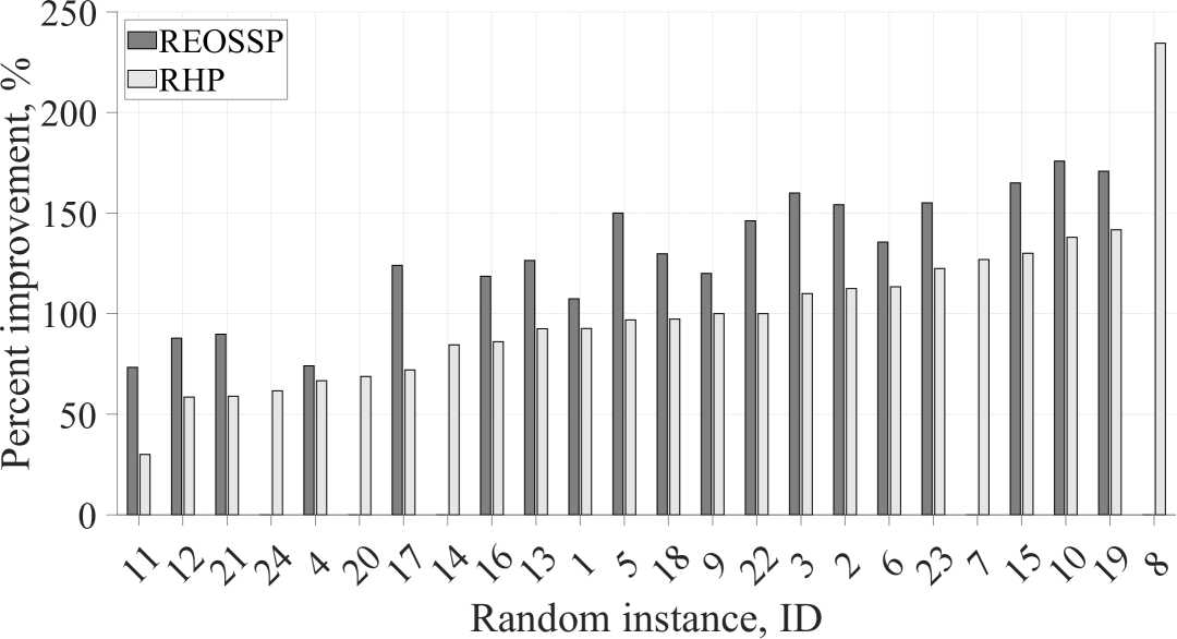
(a) Percent improvement of the REOSSP and RHP over the EOSSP.

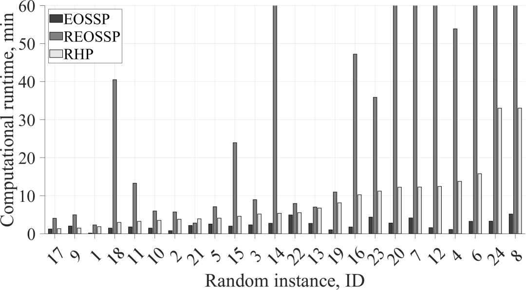
(b) Runtime of the EOSSP, REOSSP, and RHP.

Figure 6: Results of the random instances.

Statistically, the REOSSP outperforms the EOSSP with an average improvement of $129.19\text{\,}\%$ with a standard deviation of $31.27\text{\,}\%$, a minimum improvement of $0.00\text{\,}\%$ (IDs $7,8,14,20,24$), and a maximum improvement of $175.86\text{\,}\%$ (ID $10$). Similarly, the RHP outperforms the EOSSP with an average improvement of $99.53\text{\,}\%$ with a standard deviation of $39.92\text{\,}\%$, a minimum improvement of $32.63\text{\,}\%$ (ID $11$), and a maximum improvement of $234.48\text{\,}\%$ (ID $8$). Furthermore, while the RHP performs worse than the REOSSP by an average of $14.74\text{\,}\%$ with a standard deviation of $5.34\text{\,}\%$, the RHP attains significant improvement over the EOSSP in the event that the REOSSP does not obtain a feasible solution within the time limit, which occurs in IDs $7,8,14,20,24$ in which the RHP improves upon the EOSSP by an average of $115.25\text{\,}\%$.

Additionally, the runtime of the REOSSP is much greater than that of the EOSSP, while the cumulative runtime of the RHP is at maximum slightly more than half of the REOSSP runtime limit of $3600\text{\,}\mathrm{s}$, including ID $9$ where the cumulative runtime of the RHP is less than that of the EOSSP. Contrarily, the runtime of the RHP is greater than the runtime of the REOSSP in ID $21$. Statistically, the runtime of the REOSSP is $29.34\text{\,}\mathrm{m}\mathrm{i}\mathrm{n}$ on average with a standard deviation of $24.72\text{\,}\mathrm{m}\mathrm{i}\mathrm{n}$, a minimum of $2.31\text{\,}\mathrm{m}\mathrm{i}\mathrm{n}$ (ID $1$), and a maximum beyond the runtime limit (IDs $7,8,14,20,24$), while the runtime of the RHP is much lower with $8.98\text{\,}\mathrm{m}\mathrm{i}\mathrm{n}$ on average with a standard deviation of $8.52\text{\,}\mathrm{m}\mathrm{i}\mathrm{n}$, a minimum of $1.32\text{\,}\mathrm{m}\mathrm{i}\mathrm{n}$ (ID $17$), and a maximum of $33.04\text{\,}\mathrm{m}\mathrm{i}\mathrm{n}$ (ID $8$). Additionally, the minimum runtime instance of both the REOSSP and RHP results from the random parameters assigned as well as the lowest combination of $K$ and $J$, since $S$ overall only distributes the same number of time steps over a different number of stages.

Finally, the main limitation of constellation reconfigurability is the fuel cost required to perform orbital maneuvers throughout the schedule horizon, wherein the optimal schedule of the RHP uses more propellant than that of the REOSSP. The average propellant used by the REOSSP is $2.97\text{\,}\mathrm{k}\mathrm{m}\mathrm{/}\mathrm{s}$ with a standard deviation of $0.77\text{\,}\mathrm{k}\mathrm{m}\mathrm{/}\mathrm{s}$ (with the removal of IDs $7,8,14,20,24$ where no feasible solution was found). Meanwhile, the RHP is more expensive where the average propellant used is $3.66\text{\,}\mathrm{k}\mathrm{m}\mathrm{/}\mathrm{s}$ with a slightly lower standard deviation of $0.75\text{\,}\mathrm{k}\mathrm{m}\mathrm{/}\mathrm{s}$. The RHP is more expensive than the REOSSP on average as a result of the limited information presented to each subproblem, potentially leading to slightly less optimal orbital maneuvers taking place.

Overall, the average performance increase over the EOSSP by both the REOSSP and RHP shows that each solution method can greatly outperform the EOSSP despite the limited fuel budget for orbital maneuvers and additional complexity. Additionally, the value of the RHP is demonstrated through the attainment of a feasible solution well under the given time limit, especially in those cases where the REOSSP did not obtain a feasible solution. Furthermore, the RHP outperforms the REOSSP on average on account of the REOSSP instances that did not result in a feasible solution, as well as obtaining a higher maximum performance in one such instance with no REOSSP solution.

5.2 Case Study - Hurricane Sandy

In addition to the random instances, Hurricane Sandy is selected for an in-depth analysis to provide real-world data to the scheduling problems. Hurricane Sandy occurred in 2012 and struck many islands throughout the Caribbean Sea as well as the Northeastern coast of the United States, causing $233$ deaths [46] and $$65$ billion in damage [47]. Hurricane Sandy achieved Category Three status on October $25$ at 6:00 AM with $115$ mph winds at the peak [48]. Additionally, Hurricane Sandy has a since retired name, meaning that the storm’s impact was so severe that it is considered inappropriate to use the name again in the future [49].

5.2.1 Design of Case Study

For the case study, fixed schedule characteristics are selected rather than random characteristics to demonstrate realistic utilization of the scheduling problems further.

Firstly, Hurricane Sandy is depicted in Fig. 7(a) from the initial to the final occurrence of tropical storm status or higher (defined as containing winds between $39$ and $73$ mph [50]). The historical path data utilized is gathered from Ref. [48] and tracks the eye of the storm at an interval of six hours, and $T_{\text{r}}$ is set to $7.25\text{\,}\mathrm{d}\mathrm{a}\mathrm{y}\mathrm{s}$. Considering the tracking conditions, the number of targets (points along the storm path) for Hurricane Sandy is $P=29$. Additionally, binary masking is applied to $V^{k}_{tp}$ for each target in chronological order, such that target $p$ has a masking of one at time steps $t\in[1+(p-1)(T/P),p(T/P)]$ and a masking of zero otherwise. This masking condition similarly applies for $V^{sk}_{tjp}$ and $V^{\ell k}_{tjp}$ along each stage in the time horizon. The same time step size, $\Delta t=$100\text{\,}\mathrm{s}\mathrm{e}\mathrm{c}\mathrm{o}\mathrm{n}\mathrm{d}\mathrm{s}$$, is used in the case study, resulting in a total number of time steps of $T=6264$. Additionally, ground stations utilized by disaster monitoring satellites and satellite orbits suitable for EO are employed. The ground stations are assigned as two used by the Disaster Monitoring Constellation, the first being the Svalbard Satellite Station located in Sweden at $78.23\text{\,}\mathrm{d}\mathrm{e}\mathrm{g}$ North and $15.41\text{\,}\mathrm{d}\mathrm{e}\mathrm{g}$ East and the second being a satellite station located in Boecillo Spain at $41.54\text{\,}\mathrm{d}\mathrm{e}\mathrm{g}$ North and $4.70\text{\,}\mathrm{d}\mathrm{e}\mathrm{g}$ West [51]. Furthermore, a Walker-delta constellation is used as it has become a common choice in recent years for satellite configurations. The Walker-delta constellation for $K=4$ satellites is defined at an altitude of $709\text{\,}\mathrm{k}\mathrm{m}$ and takes the form $$98.18\text{\,}\mathrm{d}\mathrm{e}\mathrm{g}$:4/4/0$, where the inclination is $98.18\text{\,}\mathrm{d}\mathrm{e}\mathrm{g}$, and four satellites are located in four orbital planes with zero relative phasing between satellites. The constellation formation is selected to remain consistent with an identical FOV case in Ref. [52]. The three-dimensional locations of Hurricane Sandy over time, the two selected ground stations, and the initial satellite orbits are shown in Fig. 7(b).

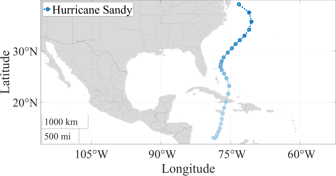
(a) Path of Hurricane Sandy.

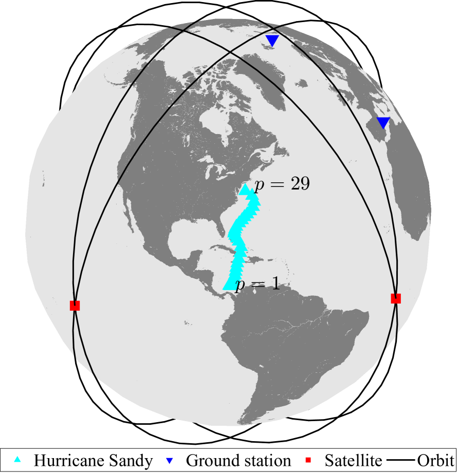
(b) Three-dimensional locations of Hurricane Sandy, ground stations, and satellites.

Figure 7: Locations of case study parameters.

Secondly, additional orbital slot options that extend to changes in the orbital plane and phase are provided. Such orbital slots allow equally spaced changes in inclination, RAAN, and phase, in which the plane-change slots extend in the positive and negative direction of the initial condition. The resultant number of orbital slot options is $J^{sk}=f(2m-1)$, where $f$ is the number of phasing options and $m$ is the number of plane-change options in each plane of either inclination or RAAN. The case studies make use of $f=15$ and $m=5$, resulting in $J^{sk}=135,\forall s\in\mathcal{S}\setminus\{0\},\forall k\in\mathcal{K}$. A demonstration of the orbital slot option space is shown in Fig. 8 of Ref. [37]. The maximum degree of separation between the initial condition and the furthest plane-change option is determined through the use of rearranged boundary value problems (assuming the entire budget, $c^{k}_{\max}$, is consumed) from Ref. [45] with an applied scaling factor of $75\text{\,}\%$ to ensure the feasibility of multiple maneuvers.

As a result of the increase in orbital slot options, additional cost computation algorithms are employed for all possible combinations of transfer types. This includes 1) phasing only, 2) inclination change only, 3) RAAN change only, 4) simultaneous inclination and RAAN change, 5) inclination change followed by phasing, 6) RAAN change followed by phasing, and 7) simultaneous inclination and RAAN change followed by phasing. As with phasing-only computations, analytical algorithms from Ref. [45] are used to compute maneuver costs. Finally, $S=8$ stages are used in the REOSSP and the RHP. All other parameters and parameter generation methods are kept identical to those in Sec. 5.1.

5.2.2 Case Study Results

The resultant schedules of the EOSSP, REOSSP, and RHP are shown in Table 3, Table 4, and Table 5, respectively. The tables depict the high-level schedule broken down by stage (in terms of the time in which a stage would occur for the EOSSP), including the number of observations, number of downlink occurrences, and number of charging occurrences, as well as the various orbital elements (inclination $i$, RAAN $\Omega$, and argument of latitude $u$, with changed elements highlighted in bold in the arrival stage) and the cost of orbital maneuvers for the REOSSP and RHP. It should be noted that Table 4 and Table 5 report the values of $i$, $\Omega$, and $u$ belonging to a specific orbital slot as defined at the start of the schedule, although propagation with SGP4 accounts for perturbations throughout the schedule duration, including in the generation of visibility and orbital maneuver cost parameters. Furthermore, the data and battery storage capacities over time are shown for the EOSSP, REOSSP, and RHP in Fig. 8, Fig. 9, and Fig. 10, respectively. The objective function values of the EOSSP, REOSSP, and RHP are $z_{\text{E}}=25$, $z_{\text{R}}=97$, and $\sum_{s=1}^{S}z_{\text{RHP}}=73$, respectively, while the figure of merit values for the EOSSP, REOSSP, and RHP are $0.80\text{\,}\mathrm{G}\mathrm{B}$, $3.20\text{\,}\mathrm{G}\mathrm{B}$, and $2.40\text{\,}\mathrm{G}\mathrm{B}$, respectively. It should be noted that despite the relatively low amount of data gathered by the constellation within the schedule horizon, the schedules only concern a single target (Hurricane Sandy) rather than any other passive monitoring occurring. Additionally, the runtime of the EOSSP, REOSSP, and RHP are $0.24\text{\,}\mathrm{m}\mathrm{i}\mathrm{n}$, $54.60\text{\,}\mathrm{m}\mathrm{i}\mathrm{n}$, and $6.65\text{\,}\mathrm{m}\mathrm{i}\mathrm{n}$, respectively. As such, the REOSSP and RHP improved upon the EOSSP in regards to the objective function value by $288.00\text{\,}\%$ and $192.00\text{\,}\%$ respectively, and in regards to the figure of merit by $300.00\text{\,}\%$ and $200.00\text{\,}\%$, respectively. Separately, the RHP performed $24.74\text{\,}\%$ and $25.00\text{\,}\%$ worse than the REOSSP regarding the objective function value and figure of merit, respectively. Meanwhile, the runtime of the RHP was only $12.18\text{\,}\%$ the runtime of the REOSSP, substantially improving computation time at a slight performance cost.

Table 3: EOSSP observation, downlink, and charge occurrence by stage.

Satellite	State	$S=1$	$S=2$	$S=3$	$S=4$	$S=5$	$S=6$	$S=7$	$S=8$
	Observations	0	0	1	0	0	0	0	0
1	Donwlinks	0	0	0	0	0	1	0	0
	Charging	0	36	40	38	38	38	37	37
	Observations	1	1	1	0	0	1	0	0
2	Donwlinks	0	0	0	0	1	0	2	1
	Charging	1	37	43	35	50	26	36	37
	Observations	0	0	0	0	0	0	1	0
3	Donwlinks	0	0	0	0	0	0	0	1
	Charging	0	37	37	39	37	37	39	38
	Observations	0	0	0	0	0	1	0	2
4	Donwlinks	0	0	0	0	0	0	1	1
	Charging	0	37	38	37	38	52	37	56

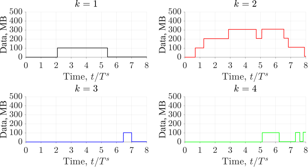
(a) EOSSP data tracking.

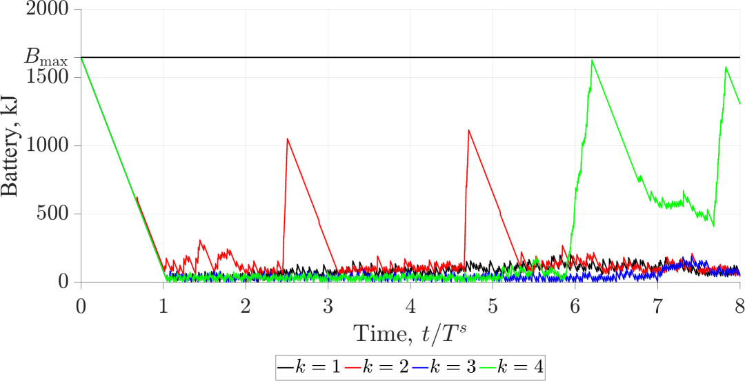
(b) EOSSP battery tracking.

Figure 8: EOSSP schedule.

The optimal schedule of the EOSSP contains only at most four observations per satellite, with two satellites only obtaining a single observation, which results in a low quantity of data and as such an objective function value of $z_{\text{E}}=25$ and a figure of merit value of $Z_{\text{E}}=$0.80\text{\,}\mathrm{G}\mathrm{B}$$. Furthermore, since the objective is to balance the observation and downlink of data, Satellite 4 achieves two observations in stage eight while only downlinking one of these observations, resulting in the satellites retaining some data that may be downlinked at a time later than the schedule horizon established. The extra data retained by Satellites 1 through 3 is a result of the previously mentioned discrepancy between the values $D_{\text{obs}}$ and $D_{\text{comm}}$, a difference of $2.50\text{\,}\mathrm{M}\mathrm{B}$ extra in $D_{\text{obs}}$. The extra data remaining onboard each satellite is reflected in Fig. 3 where Satellite 4 retains $107.50\text{\,}\mathrm{M}\mathrm{B}$, Satellite 2 retains $10.00\text{\,}\mathrm{M}\mathrm{B}$, and Satellites 1 and 3 retain $2.50\text{\,}\mathrm{M}\mathrm{B}$. In addition, the charging of each satellite is dominated by the battery constraints due to the small number of tasks performed in each stage and the large amount of power obtained via charging, as shown in Fig. 8(b). However, the large peaks shown are not determined by an eclipse of sunlight, as any eclipse only lasts at most $35\text{\,}\mathrm{m}\mathrm{i}\mathrm{n}\mathrm{u}\mathrm{t}\mathrm{e}\mathrm{s}$, slightly more than one-third of an orbital period. The reason for the large peaks shown is the large variety of feasible charging opportunities due to the low occurrence of an eclipse of sunlight, resulting in some charging schedules including the large peaks (such as Satellites 2 and 4) while others do not (such as Satellites 1 and 3).

Table 4: REOSSP observation, downlink, and charge occurrence by stage.

Satellite	State	$S=1$	$S=2$	$S=3$	$S=4$	$S=5$	$S=6$	$S=7$	$S=8$
	$i$, deg	98.18	98.18	98.18	98.18	98.18	100.33	100.33	100.33
	$\Omega$, deg	0.00	0.00	0.00	0.00	0.00	0.00	0.00	0.00
	$u$, deg	240	240	240	192	192	48	312	312
1	Observations	2	0	1	1	1	2	2	0
	Donwlinks	1	0	0	1	2	2	1	2
	Charging	3	41	33	45	40	32	37	36
	Cost, m/s	189.94	0.00	0.00	66.13	0.00	365.01	101.67	0.00
	$i$, deg	98.18	98.18	98.18	98.18	100.33	100.33	100.33	100.33
	$\Omega$, deg	90.00	90.00	90.00	90.00	90.00	90.00	90.00	90.00
	$u$, deg	336	336	336	336	72	336	240	168
2	Observations	1	1	1	1	1	1	1	1
	Donwlinks	0	1	0	2	2	1	1	1
	Charging	5	37	36	40	39	39	36	36
	Cost, m/s	145.96	0.00	0.00	0.00	347.48	101.67	101.67	16.37
	$i$, deg	98.18	98.18	98.18	98.18	98.18	98.18	98.18	98.18
	$\Omega$, deg	177.83	177.83	177.83	177.83	177.83	177.83	177.83	177.83
	$u$, deg	144	144	144	144	72	72	0	288
3	Observations	1	1	0	2	0	1	1	2
	Donwlinks	0	0	2	1	1	0	1	3
	Charging	18	48	34	33	31	31	43	40
	Cost, m/s	461.58	0.00	0.00	0.00	16.37	0.00	16.37	16.37
	$i$, deg	98.18	98.18	98.18	98.18	98.18	98.18	98.18	98.18
	$\Omega$, deg	267.83	267.83	267.83	267.83	267.83	267.83	267.83	267.83
	$u$, deg	96	96	96	96	96	24	24	24
4	Observations	2	0	2	0	1	1	0	2
	Donwlinks	1	0	1	0	0	0	3	2
	Charging	5	37	38	36	37	39	39	39
	Cost, m/s	301.57	0.00	0.00	0.00	0.00	16.37	0.00	0.00

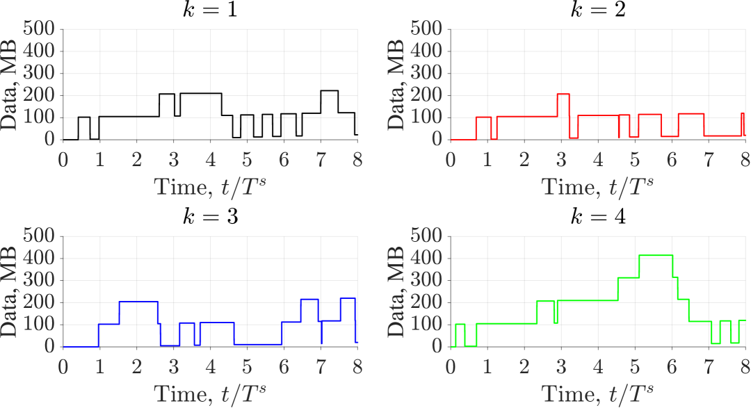
(a) REOSSP data tracking.

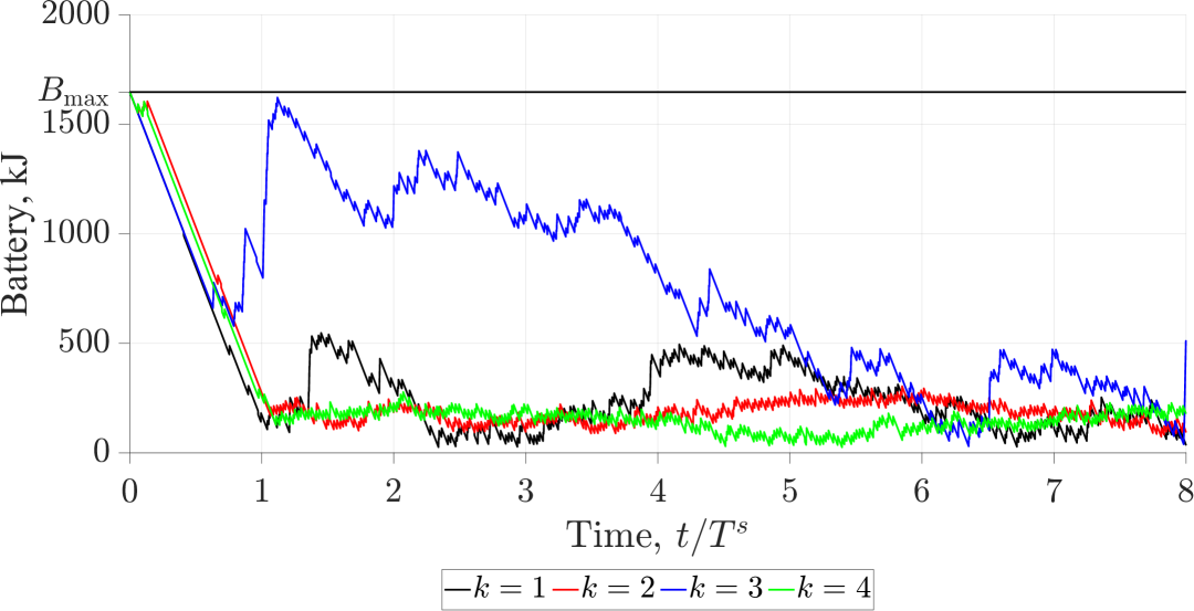
(b) REOSSP battery tracking.

Figure 9: REOSSP schedule.

The optimal schedule of the REOSSP performs significantly better than the EOSSP, by $288.00\text{\,}\%$ in terms of the objective function value and $300.00\text{\,}\%$ in terms of the figure of merit, including at least eight observations per satellite. The REOSSP also suffers from an observation with no subsequent downlink in stage eight by Satellite 4. As such, the extra data retained by each satellite is slightly higher than that retained by the satellites in the EOSSP as a result of the higher quantity of observations. Specifically reflected in Fig. 9(a), Satellite 4 retains $120.00\text{\,}\mathrm{M}\mathrm{B}$, Satellite 1 retains $22.50\text{\,}\mathrm{M}\mathrm{B}$, and Satellites 2 and 3 retain $20.00\text{\,}\mathrm{M}\mathrm{B}$. Additionally, Satellite 4 reaches the highest data storage value of $415.00\text{\,}\mathrm{M}\mathrm{B}$ within the fifth stage, wherein Satellite 4 downlinks all data before the final stage (stage eight) at which point two more observations are conducted with only a single downlink, which accounts for the extra data retained. The charging schedule, shown in Fig. 9(b), of the REOSSP may appear vastly different from the previous charging schedule; however, this variation is a result of the large variety of feasible charging solutions as the longest eclipse for this orbital maneuver pattern is similar to that of the EOSSP. Finally, the overall cost of the optimal REOSSP schedule consumes $2.26\text{\,}\mathrm{k}\mathrm{m}\mathrm{/}\mathrm{s}$, $75.48\text{\,}\%$ of the total budget provided, for a total of 15 transfers (of 32 possibilities for transfers), of which four are a plane change (two of which are inclination raising and two of which are RAAN lowering). Each Satellite, listed in order 1 through 4, consumed $722.75\text{\,}\mathrm{m}\mathrm{/}\mathrm{s}$, $713.15\text{\,}\mathrm{m}\mathrm{/}\mathrm{s}$, $510.69\text{\,}\mathrm{m}\mathrm{/}\mathrm{s}$, and $317.93\text{\,}\mathrm{m}\mathrm{/}\mathrm{s}$, which is $96.37\text{\,}\%$, $95.09\text{\,}\%$, $68.09\text{\,}\%$, and $42.39\text{\,}\%$ of each individual budget, respectively.

Table 5: RHP observation, downlink, and charge occurrence by stage.

Satellite	State	$S=1$	$S=2$	$S=3$	$S=4$	$S=5$	$S=6$	$S=7$	$S=8$
	$i$, deg	98.18	98.18	98.18	98.18	98.18	98.18	98.18	98.18
	$\Omega$, deg	0.00	357.83	357.83	357.83	357.83	357.83	357.83	357.83
	$u$, deg	240	96	24	312	312	312	312	312
1	Observations	2	1	1	0	0	0	0	0
	Donwlinks	0	0	2	2	0	0	0	0
	Charging	1	39	42	32	37	39	37	38
	Cost, m/s	189.94	523.08	16.37	16.37	0.00	0.00	0.00	0.00
	$i$, deg	93.88	93.88	93.88	93.88	93.88	93.88	93.88	93.88
	$\Omega$, deg	90.00	90.00	90.00	90.00	90.00	90.00	90.00	90.00
	$u$, deg	192	192	192	192	120	72	72	72
2	Observations	1	1	1	1	1	0	0	1
	Donwlinks	1	0	2	0	2	0	0	1
	Charging	2	54	26	33	39	36	42	34
	Cost, m/s	603.92	0.00	0.00	0.00	16.37	66.13	0.00	0.00
	$i$, deg	98.18	96.03	96.03	96.03	96.03	96.03	96.03	96.03
	$\Omega$, deg	180.00	180.00	180.00	180.00	180.00	180.00	180.00	180.00
	$u$, deg	336	168	120	120	120	120	48	336
3	Observations	1	1	0	2	0	2	0	1
	Donwlinks	0	1	0	3	0	2	0	1
	Charging	1	41	34	41	71	38	2	39
	Cost, m/s	145.96	466.27	66.13	0.00	0.00	0.00	16.37	16.37
	$i$, deg	98.18	98.18	98.18	98.18	98.18	98.18	98.18	98.18
	$\Omega$, deg	270.00	270.00	270.00	270.00	270.00	270.00	270.00	272.17
	$u$, deg	72	72	72	72	72	0	0	336
4	Observations	2	0	2	0	1	1	0	2
	Donwlinks	2	0	1	1	0	1	0	2
	Charging	1	37	39	38	72	24	22	34
	Cost, m/s	441.25	0.00	0.00	0.00	0.00	16.37	0.00	291.96

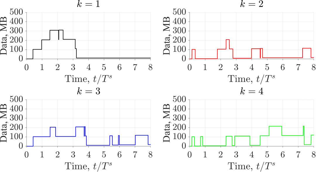
(a) REOSSP data tracking.

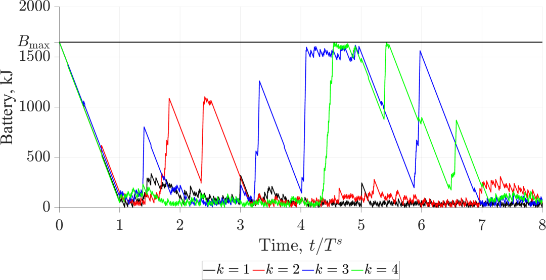
(b) REOSSP battery tracking.

Figure 10: RHP schedule.

The optimal schedule of the RHP also performs better than the EOSSP, by $192.00\text{\,}\%$ in terms of the objective function value and $200.00\text{\,}\%$ in terms of the figure of merit, but slightly worse than the REOSSP, with at least four observations per satellite. The RHP also suffers from an observation with no subsequent downlink in stage eight, indicating that this phenomenon is a result of the visibility profiles of the target and ground stations, wherein Satellite four has visibility of a target near the end of the time horizon with no visibility of ground stations afterward. Since the overall number of observations conducted by the RHP is less than that of the REOSSP, the extra data retained by each satellite is $120.00\text{\,}\mathrm{M}\mathrm{B}$, $17.50\text{\,}\mathrm{M}\mathrm{B}$, $15.00\text{\,}\mathrm{M}\mathrm{B}$, and $10.00\text{\,}\mathrm{M}\mathrm{B}$ for Satellites 4 through 1, respectively, as reflected in Fig. 10(a). An additional phenomenon occurs in Fig. 10(a), wherein data that is observed by each satellite is downlinked to a ground station much sooner than in the REOSSP and EOSSP, a result of the objective to downlink and observe being optimized for each group of two stages rather than over the accumulation of the entire time horizon. A similar phenomenon occurs in Fig. 10(b), wherein the charging of each satellite is maintained within each subproblem leading to a slightly more sporadic charging schedule when appended. Finally, the overall cost of the optimal RHP schedule is substantially more expensive than that of the REOSSP, a result of the rather small $L=1$ stage lookahead incentivizing effective yet expensive maneuvers to occur at the start of the schedule. This is displayed well in Table 5 where each satellite consumes on average $79.01\text{\,}\%$ of the maneuver budget within the first two maneuvers. Overall, the optimal RHP schedule consumes $2.89\text{\,}\mathrm{k}\mathrm{m}\mathrm{/}\mathrm{s}$, $96.43\text{\,}\%$ of the total budget provided, for a total of 15 transfers (of 32 possibilities for transfers), of which four are a plane change (two of which are inclination lowering, one of which is RAAN lowering, and one of which is RAAN raising). Each Satellite, listed in order 1 through 4, consumed $745.76\text{\,}\mathrm{m}\mathrm{/}\mathrm{s}$, $686.42\text{\,}\mathrm{m}\mathrm{/}\mathrm{s}$, $711.10\text{\,}\mathrm{m}\mathrm{/}\mathrm{s}$, and $749.58\text{\,}\mathrm{m}\mathrm{/}\mathrm{s}$, which is $99.43\text{\,}\%$, $91.52\text{\,}\%$, $94.81\text{\,}\%$, and $99.94\text{\,}\%$ of each individual budget, respectively.

Overall, the highly adaptable nature of the REOSSP and RHP enabled through reconfigurability, a diverse set of orbital slots including plane and phase changes, and the reduction in computation time via the RHP algorithm allows for performance much higher than that of the EOSSP. This effectiveness is shown through the performance of significantly more observations and downlink occurrences by each satellite relative to the EOSSP, while the RHP is much more expensive in the cost of orbital maneuvers performed while completing computation in nearly one-tenth the amount of time. Additionally, all three scheduling algorithms return a resultant schedule that obeys all constraints, including power consumption, charging, data management, and orbital maneuver budget limitations.

6 Conclusions

This paper developed a mathematical formulation to integrate constellation reconfigurability into the EOSSP through the use of MILP and previous research on the MCRP [31, 32, 25, 26, 27]. The REOSSP developed herein optimizes the schedule of a cooperative satellite constellation capable of orbital maneuvering such that the number of observations and subsequent data downlink occurrences is maximized, with a higher influence from the number of downlink occurrences. Additionally, the REOSSP considers available data storage, battery storage, and a propellant budget for orbital maneuvers, while scheduling the tasks to observe targets, downlink observed data, charge onboard batteries, and perform constellation reconfiguration at predetermined stages. Furthermore, the REOSSP is solved via the RHP, which significantly improves computational runtime compared to the REOSSP but at the cost of yielding suboptimal solutions. The novel MILP formulation of the REOSSP and the RHP allows flexible implementation, including the ability to include trajectory optimization for orbital maneuvers and optimal solutions through commercial solvers. In conjunction, a baseline EOSSP is developed and utilized for the comparison.

The computational experiments conducted in Sec. 5 demonstrate the capability of the REOSSP to outperform the EOSSP in a variety of scenarios, confirming the hypothesis set forth by previous comparative research [31, 32, 27]. Within the random instances, meant to demonstrate the flexibility of the framework under various parameters, the average percent improvement of the REOSSP and RHP over the EOSSP is $129.19\text{\,}\%$ and $99.53\text{\,}\%$ in terms of the objective function value, respectively. When applied to Hurricane Sandy the REOSSP and RHP exceed the performance of the EOSSP by $288.00\text{\,}\%$ and $192.00\text{\,}\%$ in terms of the objective function value, respectively, and $300.00\text{\,}\%$ and $200.00\text{\,}\%$ in terms of the figure of merit, respectively. While the RHP does not obtain as high of quality results as the REOSSP, in the event that the problem scale is sufficiently large so as to cause the REOSSP to be unable to converge to a feasible solution, the RHP can obtain an optimal solution to each subproblem while still significantly outperforming the EOSSP. Both the random instances and case study depict the performance increase provided by the REOSSP and RHP, while simultaneously obeying all operational and physical constraints. Overall, the implementation of constellation reconfigurability demonstrated by the REOSSP and RHP provides a greater throughput of observed data than the standard EOSSP.

Future research into the concept of constellation reconfigurability implemented in a scheduling format may take many forms. Firstly, the scope of this paper is restricted to high-thrust orbital maneuver trajectory optimization, whereas low-thrust maneuvers may allow for a lower operational cost of such a reconfigurable constellation. As such, the implementation of various low-thrust trajectory optimization theories such as those in Refs. [53, 54]. Secondly, all scheduling problems formulated in this paper assume deterministic characteristics, while many natural disasters or other observable planetary phenomena are often stochastic. Therefore, the implementation of stochastic programming similar to those in Ref. [55] to the scheduling problems developed in this paper may more accurately represent the stochastic nature of natural disaster targets. Finally, the work in this paper focuses heavily on the REOSSP and constellation reconfigurability as a whole, while previous work in Refs. [31, 32] additionally considers satellite agility, thus contributing to the potential of a similar AEOSSP formulation to be developed and used for further benchmarking of satellite agility against constellation reconfigurability.

Appendix A: Proof of Formulation Equivalence with No Orbital Maneuvers

The EOSSP and REOSSP are based on the same principles and constraints, as well as the flow of tasks and how they are linked. Furthermore, the only differences between the EOSSP and REOSSP lie within the reconfiguration of the constellation of satellites, wherein the REOSSP contributes visibility of the currently occupied orbital slot and tracks the battery required to perform orbital maneuvers. Additionally, the REOSSP assumes a battery consumption of $B_{\text{recon}}$ for each orbital maneuver performed by each satellite at the beginning of each reconfiguration stage.

Theorem 1

Let $c^{k}_{\max}=0,\forall k\in\mathcal{K}$ in the REOSSP, then $z_{\text{E}}=z_{\text{R}}$.

Proof. Suppose that for the EOSSP and REOSSP, all constant parameters such as $\Delta t$ or $K$, are identical between the scheduling problems. Note that each stage aligns in sequence along the time horizon, as reflected in Fig. 5, such that time step $t$ in stage $s$ of the REOSSP corresponds to time step $t+(s-1)T^{s}$ of the EOSSP. Furthermore, the visibility parameters $V^{sk}_{tjp}$, $G^{sk}_{tjg}$, and $H^{sk}_{tj}$ follow the same sequential alignment along the $s$ and $t$ indices, while the initial orbital element conditions of each satellite (those applied to the EOSSP for the entire time horizon) apply to the index $j=1$. Additionally, suppose that $c^{k}_{\max}=0,\forall k\in\mathcal{K}$. Finally, the number of stages $S$ and the number of orbital slots $J^{sk}$ of each stage $s$ for each satellite $k$ may remain generic.

Firstly, as reflected in Sec. 3, constraints (19c) restrict the orbital maneuvers of satellites only to those $c^{sk}_{ij}$ orbital maneuver costs that do not exceed $c^{k}_{\max}$. Since $c^{k}_{\max}=0,\forall k\in\mathcal{K}$, the only such $c^{sk}_{ij}$ that obey constraints (19c) are those where $c^{sk}_{ij}=0$, otherwise the constraints are violated. Additionally, since the orbital maneuver costs within $c^{sk}_{ij}$ are defined from orbital slot $i\in\mathcal{J}^{s-1,k}$ to orbital slot $j\in\mathcal{J}^{sk}$, a cost of zero is allotted only if $i=j,\forall k\in\mathcal{K},\forall s\in\mathcal{S}\setminus\{0\}$. Furthermore, at stage $s=1$, the orbital slot $i\in\mathcal{J}^{0k},\forall k\in\mathcal{K}$ belongs to a singleton set for each satellite, which are the initial orbital element conditions (those applied to the EOSSP for the entire time horizon). As such, the satellites within the EOSSP and REOSSP are located in the same orbital slot for the entire time horizon, wherein $i=j=1,\forall k\in\mathcal{K},\forall s\in\mathcal{S}\setminus\{0\}$. Finally, such an assignment of orbital slots within the REOSSP obeys constraints (19a), since only slot $j=1$ is occupied in stage $s=1$ such that $x^{1k}_{11}=1,\forall k\in\mathcal{K}$ and $x^{1k}_{1j}=0,\forall k\in\mathcal{K},j\neq 1$. The REOSSP additionally obeys constraints (19b) since $j^{\prime}\in\mathcal{J}^{s-1,k}=i\in\mathcal{J}^{sk}=j\in\mathcal{J}^{s+1,k}=1,\forall k\in\mathcal{K},\forall s\in\mathcal{S}\setminus\{0,S\}$ such that $x^{sk}_{11}=1,\forall k\in\mathcal{K},\forall s\in\mathcal{S}$ and $x^{sk}_{ij}=0,\forall k\in\mathcal{K},\forall s\in\mathcal{S},i\neq 1,j\neq 1$. Since each satellite never performs an orbital maneuver, it can be assumed that $B_{\text{recon}}=0$, thus eliminating the possible difference in battery power consumption between the EOSSP and REOSSP.

Secondly, as reflected in Sec. 3, constraints (20a), (20b), and (20c) assign the visibility of targets, ground stations, and the Sun, respectively, to the currently occupied orbital slot $j$ of stage $s$ for each satellite $k$. As established, the visibility parameters follow sequential alignment along the $s$ and $t$ indices, and each satellite occupies the same orbital slot $j=1$ within each stage, which is identical to that of the EOSSP. As such, the visibility of targets, ground stations, and the Sun are identically assigned to the EOSSP and REOSSP, further resulting in the identical assignment of VTWs for the tasks of target observation, data downlink to ground stations, and solar charging. Additionally, since the objective function (6) of the EOSSP and the objective function (17) of the REOSSP are functionally equivalent (again due to the sequential alignment along the $s$ and $t$ indices), and the VTWs of each task are identical, the assignment of tasks toward the same objective will also be identical. In a similar manner to the assignment of orbital slots, constraints (20d) in the REOSSP are obeyed inherently as they are in constraints (8d) in the EOSSP.

Thirdly, since it is established that the task occurrence in both the EOSSP and REOSSP are identical, and all orbital maneuver path continuity constraints of the REOSSP are obeyed, only the effect of each task on the onboard data and onboard battery storage remain to note. Firstly, since stages are sequentially aligned and the task occurrences are identical, constraints (9b) and (9c) are identical to constraints (21c) and (21d), respectively, since each set of constraints only depends on the tasks of target observation and data downlink, as well as constant values $D_{\text{comm}}$ and $D_{\text{obs}}$ that are the same between the EOSSP and REOSSP. Similarly, constraints (10b) are identical to constraints (23a) for the same reason, relating to the constant values $B_{\text{comm}}$, $B_{\text{charge}}$, $B_{\text{obs}}$, and $B_{\text{time}}$. More complex, constraints (10c) are identical to constraints (23b), (23c), and (23d). Firstly, constraints (23d) simplify through $B_{\text{recon}}=0$ to $B^{k}_{\max}\geq 0,\forall k\in\mathcal{K}$ which is implied and constraints (23c) simplify through $B_{\text{recon}}=0$ to $b^{sk}_{T^{s}}-\sum_{p\in\mathcal{P}}B_{\text{obs}}y^{sk}_{T^{s}p}-\sum_{g\in\mathcal{G}}B_{\text{comm}}q^{sk}_{T^{s}g}-B_{\text{time}}\geq 0,\forall s\in\mathcal{S}\setminus\{0,S\},\forall k\in\mathcal{K}$. Secondly, with these simplifications, constraints (23b) and constraints (23c) are the same, while constraints (23b) apply at all time steps except the final time step $T^{s}$ of each stage as well as the final time step $T^{S}$ of the final stage $S$ and constraints (23c) apply at the final time step $T^{s}$ of each stage except the final stage $S$, thus accounting for all time steps of all stages. As such, constraints (23b) and (23c) may combine to reflect $b^{sk}_{t}-\sum_{p\in\mathcal{P}}B_{\text{obs}}y^{sk}_{tp}-\sum_{g\in\mathcal{G}}B_{\text{comm}}q^{sk}_{tg}-B_{\text{time}}\geq 0,\forall s\in\mathcal{S}\setminus\{0\},\forall t\in\mathcal{T}^{s},\forall k\in\mathcal{K}$, which through the sequential alignment of stages within the time horizon accounts for all time steps, thus being identical to constraints (10c). Additionally, similar computation simplifications and compatibilities apply to the tracking constraints. Firstly, due to the sequential alignment of stages, constraints (21b) apply the same condition as constraints (21a) between each stage, while constraints (21a) apply at every time step within each stage apart from the final time step $T^{s}$, thus accounting for every time step apart from the final time step in the horizon, therefore operating identically to constraints (9a) in the EOSSP. Yet again more complex, constraints (22a), (22b), and (22c) are identical to constraints (10a). Firstly, constraints (22c) simplify through $B_{\text{recon}}=0$ to $b^{1k}_{1}=B^{k}_{\max},\forall k\in\mathcal{K}$ which is an assumption of the EOSSP and constraints (22b) simplify through $B_{\text{recon}}=0$ to $b^{s+1,k}_{1}=b^{sk}_{T^{s}}+B_{\text{charge}}h^{sk}_{T^{s}}-\sum_{p\in\mathcal{P}}B_{\text{obs}}y^{sk}_{T^{s}p}-\sum_{g\in\mathcal{G}}B_{\text{comm}}q^{sk}_{T^{s}g}-B_{\text{time}},\forall s\in\mathcal{S}\setminus\{0,S\},\forall k\in\mathcal{K}$. In this simplified form, constraints (22a) and (22b) operate in a similar manner to constraints (21b) and (21a) sequentially along each stage for all time steps apart from the final time step in the horizon, therefore operating identically to constraints (10a).

Finally, since it is established that task occurrence is identical and all constraints function identically and are obeyed, the objective functions (6) and (17) for the EOSSP and REOSSP, respectively, result in the same objective function value. Since the task occurrence is identical, the value of $q^{k}_{tg}$ and $y^{k}_{tp}$ will be the same as the value of $q^{sk}_{tg}$ and $y^{sk}_{tp}$ for similar time steps $t+(s-1)T^{s}\in\mathcal{T}$ and $t\in\mathcal{T}^{s}$, respectively. As such, the objective function values $z_{\text{E}}=z_{\text{R}}$ since each only depends on the associated number of data downlink occurrences, the number of target observations, and the constant $C$. Therefore, since all task occurrences and objective function values, are identical between the EOSSP and REOSSP under the conditions wherein $c^{k}_{\max}=0,\forall k\in\mathcal{K}$, the identicality of both formulations is maintained and proven mathematically. $\blacksquare$

In order to further validate the above proof numerically, the case study shown in Sec. 5.2 is conducted again with a change such that $c^{k}_{\max}=0,\forall k\in\mathcal{K}$ for the REOSSP. The results follow that $z_{\text{E}}=z_{\text{R}}=25$ since the satellites of the REOSSP were forced to remain in the initial condition orbital slots for the entire duration of the schedule horizon. As such, the above proof is validated using realistic target data and the same parameters and parameter generation methods as the case study in Sec. 5.2.

References

- Crocetti et al. [2020] Crocetti, L., Forkel, M., Fischer, M., Jurečka, F., Grlj, A., Salentinig, A., Trnka, M., Anderson, M., Ng, W.-T., Kokalj, Z., and et al., “Earth observation for agricultural drought monitoring in the Pannonian Basin (Southeastern Europe): Current State and future directions,” Regional Environmental Change, Vol. 20, No. 4, 2020, p. 123. 10.1007/s10113-020-01710-w.
- Soldi et al. [2021] Soldi, G., Gaglione, D., Forti, N., Simone, A. D., Daffinà, F. C., Bottini, G., Quattrociocchi, D., Millefiori, L. M., Braca, P., Carniel, S., Willett, P., Iodice, A., Riccio, D., and Farina, A., “Space-Based Global Maritime Surveillance. Part I: Satellite Technologies,” IEEE Aerospace and Electronic Systems Magazine, Vol. 36, No. 9, 2021, pp. 8–28. 10.1109/MAES.2021.3070862.
- Prakash et al. [2020] Prakash, M., Ramage, S., Kavvada, A., and Goodman, S., “Open Earth Observations for Sustainable Urban Development,” Remote Sensing, Vol. 12, No. 10, 2020. 10.3390/rs12101646.
- Chien et al. [2019] Chien, S., Mclaren, D., Doubleday, J., Tran, D., Tanpipat, V., and Chitradon, R., “Using Taskable Remote Sensing in a Sensor Web for Thailand Flood Monitoring,” Journal of Aerospace Information Systems, Vol. 16, No. 3, 2019, pp. 107–119. 10.2514/1.I010672.
- Parselia et al. [2019] Parselia, E., Kontoes, C., Tsouni, A., Hadjichristodoulou, C., Kioutsioukis, I., Magiorkinis, G., and Stilianakis, N. I., “Satellite Earth Observation Data in Epidemiological Modeling of Malaria, Dengue and West Nile Virus: A Scoping Review,” Remote Sensing, Vol. 11, No. 16, 2019. 10.3390/rs11161862.
- Cho et al. [2018] Cho, D.-H., Kim, J.-H., Choi, H.-L., and Ahn, J., “Optimization-Based Scheduling Method for Agile Earth-Observing Satellite Constellation,” Journal of Aerospace Information Systems, Vol. 15, No. 11, 2018, pp. 611–626. 10.2514/1.I010620.
- Herrmann and Schaub [2023] Herrmann, A., and Schaub, H., “Reinforcement learning for the agile earth-observing satellite scheduling problem,” IEEE Transactions on Aerospace and Electronic Systems, 2023. 10.1109/taes.2023.3251307.
- Eddy and Kochenderfer [2021] Eddy, D., and Kochenderfer, M. J., “A Maximum Independent Set Method for Scheduling Earth-Observing Satellite Constellations,” Journal of Spacecraft and Rockets, Vol. 58, No. 5, 2021, pp. 1416–1429. 10.2514/1.A34931.
- Chatterjee and Tharmarasa [2022] Chatterjee, A., and Tharmarasa, R., “Reward Factor-Based Multiple Agile Satellites Scheduling With Energy and Memory Constraints,” IEEE Transactions on Aerospace and Electronic Systems, Vol. 58, No. 4, 2022, pp. 3090–3103. 10.1109/TAES.2022.3146115.
- Chen et al. [2019] Chen, X., Reinelt, G., Dai, G., and Spitz, A., “A mixed integer linear programming model for multi-satellite scheduling,” European Journal of Operational Research, Vol. 275, No. 2, 2019, pp. 694–707. 10.1016/j.ejor.2018.11.058.
- Herrmann and Schaub [2022] Herrmann, A. P., and Schaub, H., “Monte Carlo tree search methods for the Earth-observing satellite scheduling problem,” Journal of Aerospace Information Systems, Vol. 19, No. 1, 2022, p. 70–82. 10.2514/1.i010992.
- Lemaitre et al. [2002] Lemaitre, M., Verfaillie, G., Jouhaud, F., Lachiver, J.-M., and Bataille, N., “Selecting and scheduling observations of agile satellites,” Aerospace Science and Technology, Vol. 6, No. 5, 2002, pp. 367–381. 10.1016/S1270-9638(02)01173-2.
- Lee et al. [2024a] Lee, K., Kim, D.-J., Chung, D.-W., and Lee, S., “Optimal Mission Planning for Multiple Agile Satellites Using Modified Dynamic Programming,” Journal of Aerospace Information Systems, Vol. 21, No. 3, 2024a, pp. 279–289. 10.2514/1.I011270.
- Wang et al. [2019] Wang, X., Han, C., Zhang, R., and Gu, Y., “Scheduling Multiple Agile Earth Observation Satellites for Oversubscribed Targets Using Complex Networks Theory,” IEEE Access, Vol. 7, 2019, pp. 110605–110615. 10.1109/ACCESS.2019.2925704.
- Kim et al. [2020] Kim, J., Ahn, J., Choi, H.-L., and Cho, D.-H., “Task Scheduling of Agile Satellites with Transition Time and Stereoscopic Imaging Constraints,” Journal of Aerospace Information Systems, Vol. 17, No. 6, 2020, pp. 285–293. 10.2514/1.I010775.
- Peng et al. [2020] Peng, G., Song, G., Xing, L., Gunawan, A., and Vansteenwegen, P., “An Exact Algorithm for Agile Earth Observation Satellite Scheduling with Time-Dependent Profits,” Computers & Operations Research, Vol. 120, 2020, p. 104946. 10.1016/j.cor.2020.104946.
- de Weck et al. [2008] de Weck, O. L., Scialom, U., and Siddiqi, A., “Optimal reconfiguration of satellite constellations with the auction algorithm,” Acta Astronautica, Vol. 62, No. 2, 2008, pp. 112–130. 10.1016/j.actaastro.2007.02.008.
- Lee and Ho [2023] Lee, H., and Ho, K., “Regional Constellation Reconfiguration Problem: Integer Linear Programming Formulation and Lagrangian Heuristic Method,” Journal of Spacecraft and Rockets, Vol. 60, No. 6, 2023, pp. 1828–1845. 10.2514/1.A35685.
- Paek et al. [2019] Paek, S. W., Kim, S., and de Weck, O., “Optimization of Reconfigurable Satellite Constellations Using Simulated Annealing and Genetic Algorithm,” Sensors, Vol. 19, No. 4, 2019. 10.3390/s19040765.
- Chen et al. [2015] Chen, Y., Mahalec, V., Chen, Y., Liu, X., He, R., and Sun, K., “Reconfiguration of satellite orbit for cooperative observation using variable-size multi-objective differential evolution,” European Journal of Operational Research, Vol. 242, No. 1, 2015, pp. 10–20. 10.1016/j.ejor.2014.09.025.
- Anderson et al. [2022] Anderson, J. F., Cardin, M.-A., and Grogan, P. T., “Design and analysis of flexible multi-layer staged deployment for satellite mega-constellations under demand uncertainty,” Acta Astronautica, Vol. 198, 2022, p. 179–193. 10.1016/j.actaastro.2022.05.022.
- Zuo et al. [2022] Zuo, X., Bai, X., Xu, M., Li, M., Zhou, J., Yu, L., and Zhang, J., “Satellite Constellation Reconfiguration Using Surrogate-Based Optimization,” Journal of Aerospace Engineering, Vol. 35, No. 4, 2022, p. 04022043. 10.1061/(ASCE)AS.1943-5525.0001438.
- Lee and Ho [2021] Lee, H., and Ho, K., “A Lagrangian Relaxation-Based Heuristic Approach to Regional Constellation Reconfiguration Problem,” AAS/AIAA Astrodynamics Specialist Conference, 2021.
- Lee and Ho [2020] Lee, H., and Ho, K., “Binary Integer Linear Programming Formulation for Optimal Satellite Constellation Reconfiguration,” AAS/AIAA Astrodynamics Specialist Conference, 2020.
- Lee et al. [2022] Lee, H., Chen, H., and Ho, K., “Maximizing Observation Throughput via Multi-Stage Satellite Constellation Reconfiguration,” AAS/AIAA Astrodynamics Specialist Conference, 2022.
- Lee and Liu [2023] Lee, H., and Liu, Z., “A Novel Formulation for the Multi-Stage Satellite Constellation Reconfiguration Problem: Initial Results,” 33rd AAS/AIAA Space Flight Mechanics Meeting, 2023.
- Lee et al. [2024b] Lee, H., Williams Rogers, D. O., Pearl, B. D., Chen, H., and Ho, K., “Deterministic Multistage Constellation Reconfiguration Using Integer Programming and Sequential Decision-Making Methods,” Journal of Spacecraft and Rockets, 2024b. 10.2514/1.A35990, (article in advance).
- He et al. [2020] He, X., Li, H., Yang, L., and Zhao, J., “Reconfigurable Satellite Constellation Design for Disaster Monitoring Using Physical Programming,” International Journal of Aerospace Engineering, Vol. 2020, 2020, p. 8813685. 10.1155/2020/8813685.
- McGrath and Macdonald [2019] McGrath, C. N., and Macdonald, M., “General Perturbation Method for Satellite Constellation Reconfiguration Using Low-Thrust Maneuvers,” Journal of Guidance, Control, and Dynamics, Vol. 42, No. 8, 2019, pp. 1676–1692. 10.2514/1.G003739.
- Morgan et al. [2023] Morgan, S. J., McGrath, C. N., and de Weck, O. L., “Optimization of multispacecraft maneuvers for mobile target tracking from low Earth orbit,” Journal of Spacecraft and Rockets, Vol. 60, No. 2, 2023, p. 581–590. 10.2514/1.a35457.
- Pearl et al. [2023] Pearl, B., Gold, L., and Lee, H., “Comparing the Effectiveness of Agility and Reconfigurability in Earth Observation Satellite Systems for Disaster Response,” AAS/AIAA Astrodynamics Specialist Conference, 2023.
- Pearl et al. [2025a] Pearl, B. D., Gold, L. P., and Lee, H., “Benchmarking Agility and Reconfigurability in Satellite Systems for Tropical Cyclone Monitoring,” Journal of Spacecraft and Rockets, 2025a. 10.2514/1.A36177, (article in advance).
- Candela et al. [2023] Candela, A., Swope, J., and Chien, S. A., “Dynamic Targeting to Improve Earth Science Missions,” Journal of Aerospace Information Systems, Vol. 20, No. 11, 2023, pp. 679–689. 10.2514/1.I011233.
- Swope et al. [2024] Swope, J., Chien, S., Bosch-Lluis, X., Dunkel, E., Yue, Q., Ogut, M., Ramos, I., Kangaslahti, P., Deal, W., and Cooke, C., “Storm Classification and Dynamic Targeting for a Smart Ice Cloud Sensing Satellite,” Journal of Aerospace Information Systems, Vol. 21, No. 12, 2024, pp. 958–971. 10.2514/1.I011318.
- Wang et al. [2023] Wang, X., Zhao, F., Shi, Z., and Jin, Z., “Deep Reinforcement Learning-Based Periodic Earth Observation Scheduling for Agile Satellite Constellation,” Journal of Aerospace Information Systems, Vol. 20, No. 8, 2023, pp. 508–519. 10.2514/1.I011209.
- Morgan et al. [2014] Morgan, D., Chung, S.-J., and Hadaegh, F. Y., “Model Predictive Control of Swarms of Spacecraft Using Sequential Convex Programming,” Journal of Guidance, Control, and Dynamics, Vol. 37, No. 6, 2014, pp. 1725–1740. 10.2514/1.G000218.
- Pearl et al. [2025b] Pearl, B. D., Miller, J. M., and Lee, H., “Developing the Reconfigurable Earth Observation Satellite Scheduling Problem,” AIAA SCITECH 2025 Forum, 2025b. 10.2514/6.2025-0589.
- Huang et al. [2021] Huang, Y., Mu, Z., Wu, S., Cui, B., and Duan, Y., “Revising the Observation Satellite Scheduling Problem Based on Deep Reinforcement Learning,” Remote Sensing, Vol. 13, No. 12, 2021. 10.3390/rs13122377.
- MATLAB [2024] MATLAB, 24.2.0.2806996 (R2024b) Update 3, The MathWorks Inc., Natick, Massachusetts, 2024.
- Löfberg [2004] Löfberg, J., “YALMIP : a toolbox for modeling and optimization in MATLAB,” 2004 IEEE International Conference on Robotics and Automation (IEEE Cat. No.04CH37508), Taipei, Taiwan, 2004, pp. 284–289. 10.1109/CACSD.2004.1393890.
- eoPortal [2012] eoPortal, “DMC-3 (disaster monitoring constellation-3),” https://www.eoportal.org/satellite-missions/dmc-3, 05 2012. Last accessed February 03, 2025.
- Maccherone and Frazier [2015] Maccherone, B., and Frazier, S., “Moderate Resolution Imaging Spectroradiometer,” https://modis.gsfc.nasa.gov/about/specifications.php, 2015. Last accessed February 03, 2025.
- Bradhorst [1985] Bradhorst, H. W., “Technologies,” https://nss.org/settlement/nasa/spaceresvol2/technologies.html, 1985. Last accessed February 03, 2025.
- Woodburn [2000] Woodburn, J., “Effects of eclipse boundary crossings on the numerical integration of orbit trajectories,” Astrodynamics Specialist Conference, 2000. 10.2514/6.2000-4027.
- Vallado [2022] Vallado, D., Fundamentals of Astrodynamics and Applications, Space technology library, Microcosm Press, 2022, Chap. 6, pp. 321–428.
- Diakakis et al. [2015] Diakakis, M., Deligiannakis, G., Katsetsiadou, K., and Lekkas, E., “Hurricane Sandy mortality in the Caribbean and Continental North America,” Disaster Prevention and Management, Vol. 24, No. 1, 2015, p. 132–148. 10.1108/dpm-05-2014-0082.
- National Hurricane Center [2018] National Hurricane Center, “Costliest U.S. tropical cyclones tables updated,” https://www.nhc.noaa.gov/news/UpdatedCostliest.pdf, 01 2018. Last accessed February 03, 2025.
- Weather Underground [2024] Weather Underground, “Hurricane Archive,” https://www.wunderground.com/hurricane/archive, 2024. Last accessed February 03, 2025.
- National Hurricane Center and Central Pacific Hurricane Center [2024] National Hurricane Center, and Central Pacific Hurricane Center, “Tropical Cyclone Naming History and Retired Names,” https://www.nhc.noaa.gov/aboutnames_history.shtml, 2024. Last accessed February 03, 2025.
- US Department of Commerce and NOAA [2022] US Department of Commerce, and NOAA, “Tropical definitions,” https://www.weather.gov/mob/tropical_definitions, 05 2022. Last accessed February 03, 2025.
- European Space Agency [2024] European Space Agency, “GEOSAT-1 Overview,” https://earth.esa.int/eogateway/missions/geosat-1/description, 2024. Last accessed February 03, 2025.
- Nag et al. [2015] Nag, S., LeMoigne, J., Miller, D. W., and de Weck, O., “A framework for orbital performance evaluation in Distributed Space Missions for Earth Observation,” 2015 IEEE Aerospace Conference, 2015. 10.1109/aero.2015.7119227.
- Sims and Flanagan [2000] Sims, J., and Flanagan, S., “Preliminary Design of Low-Thrust Interplanetary Missions,” Advances in the Astronautical Sciences, Vol. 103, 2000.
- Shannon et al. [2020] Shannon, J. L., Ozimek, M. T., Atchison, J. A., and Hartzell, C. M., “Q-Law Aided Direct Trajectory Optimization of Many-Revolution Low-Thrust Transfers,” Journal of Spacecraft and Rockets, Vol. 57, No. 4, 2020, pp. 672–682. 10.2514/1.A34586.
- Hoskins [2024] Hoskins, A. B., “Optimized Observation of an At Launch Unknown Ground Target Within Sensor Field of View,” 2024 IEEE Aerospace Conference, 2024, pp. 1–9. 10.1109/AERO58975.2024.10521384.