Instabilities of internal gravity waves
in the two-dimensional Boussinesq system

Abstract.

We consider a two-dimensional, incompressible, inviscid fluid with variable density, subject to the action of gravity. Assuming a stable equilibrium density profile, we adopt the so-called Boussinesq approximation, which neglects density variations in all terms except those involving gravity. This model is widely used in the physical literature to describe internal gravity waves.

In this work, we prove a modulational instability result for such a system: specifically, we show that the linearization around a small-amplitude travelling wave admits at least one eigenvalue with positive real part, bifurcating from double eigenvalues of the linear, unperturbed equations. This can be regarded as the first rigorous justification of the Parametric Subharmonic Instability (PSI) of inviscid internal waves, wherein energy is transferred from an initially excited primary wave to two secondary waves with different frequencies. Our approach uses Floquet–Bloch decomposition and Kato’s similarity transformations to compute rigorously the perturbed eigenvalues without requiring boundedness of the perturbed operator - differing fundamentally from prior analyses involving viscosity.

Notably, the inviscid setting is especially relevant in oceanographic applications, where viscous effects are often negligible.
Keywords: Boussinesq equations; internal gravity waves; spectral instability; modulational instability; parametric subharmonic instability.

1. Introduction

We consider two-dimensional, incompressible fluids stratified under the Boussinesq approximation, where density variation $\rho=\rho(t,x,y)$ is a small fluctuation of its (constant) average $\rho_{0}$, and does not affect inertial terms; see, for example, [23, Section 2] for an introduction and [36, 5] for a discussion on the Boussinesq approximation. In the simplest setting, density at the hydrostatic equilibrium is given by an affine, stable profile $\overline{\rho}(y)$ with $\overline{\rho}^{\prime}(y)=\beta<0$, and density variation takes the form $\rho=\overline{\rho}(y)+\frac{\rho_{0}}{\mathfrak{g}}b$, where $\mathfrak{g}$ is gravity acceleration constant. The two-dimensional inviscid Boussinesq equations for (stably) stratified fluids in ${\mathbb{R}}^{2}$ are given below (see (1.5) in [16]):

$$\partial_{t}u+\partial_{x}P+(\mathbf{u}\cdot\nabla)u =0,$$

$$\partial_{t}v+b+\partial_{y}P+(\mathbf{u}\cdot\nabla)v =0,$$

$$\partial_{t}b-N^{2}v+(\mathbf{u}\cdot\nabla)b =0,$$

(1.1) $$\partial_{x}u+\partial_{y}v =0,$$

where $\mathbf{u}=(u,v)=(u(t,\bm{x}),v(t,\bm{x})):{\mathbb{R}}^{+}\times{\mathbb{R}}^{2}\to{\mathbb{R}}^{2}$, $\bm{x}=(x,y)$, is the (divergence-free) velocity field, $P=P(t,\bm{x}):{\mathbb{R}}^{+}\times{\mathbb{R}}^{2}\to{\mathbb{R}}$ is the pressure,

(1.2) $$N^{2} :=-\frac{\mathfrak{g}\overline{\rho}^{\prime}(y)}{\rho_{0}}$$

is the so-called Brunt–Väisälä frequency, which represents the maximum frequency of oscillations of internal gravity waves supported by the above system. Introducing the vorticity

(1.3) $$\omega :=\partial_{x}v-\partial_{y}u\,=\,-\Delta\psi,$$

system (1) can be written in vorticity-stream formulation (see Sec. 2 of [1]; see also [7]):

(1.4) $$\begin{cases}\partial_{t}b=-\,N^{2}\,\partial_{x}\psi-\{b,\psi\},\\ \partial_{t}\omega=-\partial_{x}b-\{\omega,\psi\},\end{cases}\quad-\Delta\psi=\omega,$$

where for any couple of functions $f,g$ we define the Poisson brackets $\{f,g\}=\partial_{x}f\partial_{y}g-\partial_{y}f\partial_{x}g$.

State of the art on the Boussinesq equations

From a mathematical perspective, the analysis of the Boussinesq system (1) has recently attracted considerable attention. Among the outstanding open problems is the question of whether solutions originating from smooth, finite-energy initial data can develop finite-time singularities in the case $N=0$; see the recent blow-up result for $C^{1,\alpha}$ velocity fields in the unstable setting [27]. Even when the linearized system at the origin is spectrally stable — as is the case for $N^{2}\neq 0$ [26] — the issue of global regularity versus finite-time blow-up for smooth solutions remains unresolved; see [32] for recent progress in this direction.

Beyond the question of global existence versus blow-up, another important aspect of the Boussinesq system concerns the possible growth of Sobolev norms over time, which is closely connected to the formation of small scales and turbulent behaviors; see [34]. In the inviscid setting considered here, algebraic-in-time growth of the density gradient $\|\nabla b\|_{L^{2}}$ or the vorticity $\|\omega\|_{L^{2}}$, with $\omega=\nabla\cdot\mathbf{u}^{\perp}$, has been demonstrated under suitable symmetry assumptions on the initial data [34], and also in the presence of a background shear flow [3].

Internal waves and the scope of this work

The Boussinesq equations for stratified fluids describe the propagation of internal gravity waves, which play a crucial role in stratified fluids, contributing significantly to ocean mixing [23]. The propagation and reflection of internal waves are by now fairly well understood, with several mathematical results available; see, for instance, [25, 14, 26]. Nonlinear phenomena, such as energy transfers, dissipation mechanisms, and related turbulent behaviors remain active areas of investigation; see the recent review [40].

This paper provides the first rigorous mathematical study of instabilities in internal gravity waves in the inviscid setting, focusing on growth mechanisms generated by resonant interactions under small-amplitude perturbations. A preliminary mathematical study in the viscous case was provided in [15].

Here, we investigate the Parametric Subharmonic Instability (PSI) of inviscid internal waves - the inviscid counterpart of the Triadic Resonant Instability (TRI); see [23, Section 3.5]. Remarkably, the inviscid setting is particularly relevant for oceanographic applications, where viscosity is often negligible [23]. In the 1970s, internal gravity waves were discovered to be unstable to infinitesimal perturbations, which can grow to form temporal and spatial resonant triads [24]. The convection term in the Boussinesq system plays a crucial role by enabling energy transfer among waves of different frequencies. Specifically, under the effect of nonlinearities, a primary wave perturbed by small disturbances can transfer part of its energy to two secondary waves of lower frequency (subharmonics). Thus, TRI and PSI represent direct energy transfer mechanisms, without the need for turbulent cascade. TRI or PSI arises when three waves of wavevectors $\mathbf{k}_{j}$ and time frequency $\Omega(\mathbf{k}_{j})$, $j\in\{1,2,3\}$ interact resonantly, satisfying the relations $\sum_{j=1}^{3}\Omega(\mathbf{k}_{j})=0$ for the frequencies and $\sum_{j=1}^{3}\mathbf{k}_{j}=0$ for the wavevectors [23]. This instability has been observed in laboratory experiments [4, 31] and confirmed by oceanic field measurements [28, 37]. Interestingly, recent physics studies [2] have used Floquet methods to study PSI and to identify a novel “broadband” instability at large Floquet parameters.

Although TRI has previously been studied in the presence of viscosity, our focus here is its inviscid counterpart, PSI [23, Section 3.1]. The earlier work [15] used classical perturbation theory to construct approximate eigenvalues (quasi-modes) in the viscous case. However, that approach requires the perturbation to be relatively compact or bounded - a condition violated in the inviscid case, where the unperturbed operator is of zeroth order and the perturbation (convection term) is of first order. To overcome this, we develop a new framework for the inviscid setting, based on Floquet-Bloch decomposition and Kato’s similarity transformations, which allows to rigorously compute perturbed eigenvalues without assuming boundedness of the perturbation. This approach fundamentally differs from prior work involving viscosity [15], and provides the first rigorous justification of PSI for inviscid internal waves.

Our main result reads as follows.

Theorem 1.

There exists $\epsilon_{0}>0$ such that, for all $0<\epsilon\leq\epsilon_{0}$, linearizing equations (1.4) near a plane wave solution of wavevector ${\underline{\bm{k}}}=({\mathtt{m}},{\mathtt{n}})^{T}\in\mathbb{Z}^{2}$ with ${\mathtt{m}},{\mathtt{n}}>0$ and small amplitude of the form

$$\begin{pmatrix}b(t,\bm{x})\\ \omega(t,\bm{x})\end{pmatrix} =\epsilon\bm{U}({\underline{\bm{k}}})e^{\mathrm{i}\left({\underline{\bm{k}}}\cdot\bm{x}-\Omega({\underline{\bm{k}}})t\right)}+\text{c.c.},\quad\bm{U}({\underline{\bm{k}}})\in\mathbb{C}^{2},\qquad\Omega({\underline{\bm{k}}})=N\frac{{\mathtt{m}}}{|{\underline{\bm{k}}}|},$$

the corresponding linearized operator $\mathcal{L}_{\epsilon}$ has at least one unstable eigenvalue $\lambda$ with $\mathrm{Re}(\lambda)>0$.

Historically, wave–wave interactions have been studied via formal weakly nonlinear expansions, which allow for the formal computation of the real part of unstable eigenvalues [23].

Here, we perform a rigorous analysis of the spectrum of the inviscid Boussinesq equations linearized around a background (primary) wave, and we rigorously prove the existence of eigenvalues with strictly positive real part. This confirms the expressions previously obtained in the literature, as discussed in Section 6. Our approach is based on modulational instability, a ubiquitous phenomenon whereby traveling wave solutions of nonlinear dispersive equations become unstable under long-wave perturbations.

In fluid dynamics, modulational instability traces back to the pioneering works of Benjamin and Feir, Zakharov, Lighthill, and McLean [6, 8, 41, 35, 38] on the instability of Stokes waves in irrotational water waves.

This problem has recently attracted renewed interest due to the development of new analytical tools that allow for the rigorous computation of portions of the unstable spectrum of the linearized water wave operator. These advancements have been made both near the origin [19, 39, 10, 11, 12, 29], away from the origin [20, 13, 9, 29], and even in the context of 3D water waves [22, 21, 30].

In this paper, we adapt the ideas in [10, 9], with some important differences. First, the Boussinesq equations in vorticity form admit a non-canonical Hamiltonian structure [1]; as a result, the linearized Boussinesq operator around an internal wave (see (2.5)) does not appear to be linearly Hamiltonian. Therefore, we use only spectral projectors to compute the matrix representing the action of the linearized operator on a two-dimensional invariant subspace, rather than employing Kato’s transformation operator (see Lemma 3.2). However, the linearized operator turns out to be reversible, and we exploit this structure.

Another important difference with respect to [10, 9] concerns the spectral structure of the unperturbed linearized operator $\mathcal{L}_{\bm{\mu},0}$ defined in (2.14). Specifically, we take the Floquet parameter $\bm{\mu}\in\mathbb{R}^{2}\setminus\{\bm{0}\}$ to enforce the resonance condition

(1.5) $$\Omega({\underline{\bm{k}}})-\Omega({\underline{\bm{k}}}+\bm{\mu})=\Omega(\bm{\mu}),$$

which is inspired by the TRI and PSI phenomena, where energy is transferred from a primary wave to two secondary waves. In Lemma 2.5, we analytically characterize the set $\mathcal{R}_{{\underline{\bm{k}}}}$ of values of $\bm{\mu}$ that satisfy (1.5).

The key observation is that whenever $\bm{\mu}\in\mathcal{R}_{{\underline{\bm{k}}}}$, the operator ${\mathcal{L}}_{\bm{\mu},0}$ possesses, as an unbounded operator on $L^{2}({\mathbb{T}}^{2})$, a purely imaginary eigenvalue $\lambda^{+}$ with multiplicity at least $2$. However, due to the higher dimensionality of ${\mathbb{T}}^{2}$, this multiplicity may be much greater than two, complicating the bifurcation analysis.

To address this issue, we exploit the fact that the Boussinesq plane wave solutions only involve Fourier coefficients at $\pm{\underline{\bm{k}}}$. This implies that the operator $\mathcal{L}_{\bm{\mu},0}$ leaves invariant the subspace $H^{1}_{{\underline{\bm{k}}}}$, consisting of functions supported only on wavevectors proportional to ${\underline{\bm{k}}}$. We then prove that, when restricted to $H^{1}_{{\underline{\bm{k}}}}$, and for any $\bm{\mu}\in\mathcal{R}_{{\underline{\bm{k}}}}$ (up to a discrete set), the eigenvalue $\lambda^{+}$ is isolated and has algebraic multiplicity exactly $2$ (see Proposition 2.7). This reduction enables us to apply the perturbative theory of isolated eigenvalues (see Section 3), ultimately reducing the problem to the computation of the eigenvalues of a $2\times 2$ matrix $\mathtt{L}(\bm{\mu},\epsilon)$ (see (3.7)). In Theorem 2, we show that these eigenvalues are given by

$$\lambda^{\pm}(\bm{\mu},\epsilon)=\lambda^{+}+{\rm i}\,\mathcal{O}(\epsilon^{2})\pm\epsilon\sqrt{\mathtt{e}(\bm{\mu})+\mathcal{O}(\epsilon)},$$

and we provide an explicit expression for the real-valued function $\mathtt{e}(\bm{\mu})$, together with its asymptotics for both $|\bm{\mu}|\ll 1$ and $|\bm{\mu}|\gg 1$, showing that it is strictly positive in both regimes.

In Section 4, we compute the small-$\epsilon$ expansions of the entries of the matrix $\mathtt{L}(\bm{\mu},\epsilon)$ using so-called entanglement coefficients, based on the jets of the operator ${\mathscr{L}}_{\bm{\mu},\epsilon}:=\mathcal{L}_{\bm{\mu},\epsilon}|_{H^{1}_{{\underline{\bm{k}}}}}$. By generalizing the approach of [9], we define, for each $\bm{\kappa}\in{\underline{\bm{k}}}\mathbb{Z}$ and for any operator $A$ acting on $H^{1}_{{\underline{\bm{k}}}}$, the projected operators $A^{[\bm{\kappa}]}$ whose matrix coefficients are supported on the bands where $(j_{2}-j_{1}){\underline{\bm{k}}}=\bm{\kappa}$, for $j_{1},j_{2}\in\mathbb{Z}$ (see (4.10)). This framework allows us to exploit structural properties of the jets of ${\mathscr{L}}_{\bm{\mu},\epsilon}$ and leads to a more efficient computation of the entanglement coefficients.

Notation and conventions

We list the notation and conventions used throughout the paper: for a given vector $\bm{f}=(f_{1},f_{2})^{T}$, we use the notation $\bm{f}^{\perp}:=(f_{2},-f_{1})^{T}$; similarly, $\operatorname{\nabla^{\perp}}:=(\partial_{y},-\partial_{x})^{T}$; we denote by $\mathcal{O}({\epsilon}^{n})$ an analytic function that, for some $C>0$ and for any small ${\epsilon}$, satisfy $|\mathcal{O}({\epsilon}^{n})|\leq C|{\epsilon}|^{n}$; we denote by $r({\epsilon}^{n})$ a function $\mathcal{O}({\epsilon}^{n})$ which is real-valued; for any $k\in\mathbb{N}$, ${\mathcal{O}}_{k}$ is an operator from $H^{1}(\mathbb{T}^{2},\mathbb{C}^{2})$ to $L^{2}(\mathbb{T}^{2},\mathbb{C}^{2})$, of size ${\epsilon}^{k}$; for any couple of functions $f,g$, the Poisson brackets $\{f,g\}=\partial_{x}f\partial_{y}g-\partial_{y}f\partial_{x}g$.

2. Internal plane waves and the linearized system

System (1.4) supports the propagation of traveling wave solutions - called internal gravity waves - of the form

(2.1) $$b(t,\bm{x})=\check{b}(\bm{x}-\bm{c}t), \;\;\omega(t,\bm{x})=\check{\omega}(\bm{x}-\bm{c}t),\quad\bm{c}=(c_{1},c_{2})^{\top}\in{\mathbb{R}}^{2}\$$

where the profiles $\check{b}(\bm{x})$ and $\check{\omega}(\bm{x})$ are plane waves. The following result can be easily verified.

Proposition 2.1.

For any $\epsilon>0$ and $\underline{\bm{k}}=({\mathtt{m}},{\mathtt{n}})^{T}\in{\mathbb{Z}}^{2}\setminus\{\bm{0}\}$,

$$b_{\epsilon}(\bm{x}) :=\epsilon\,\sin(\underline{\bm{k}}\cdot\bm{x}),\qquad\omega_{\epsilon}(\bm{x}):=\epsilon\,\frac{|{\underline{\bm{k}}}|}{N}\,\sin(\underline{\bm{k}}\cdot\bm{x}),\;\;$$

(2.2) $$\underline{\bm{c}} :=\frac{N\,{\mathtt{m}}}{|\underline{\bm{k}}|^{3}}\,\underline{\bm{k}},\qquad\psi_{\epsilon}(\bm{x}):=\epsilon\,\frac{1}{N\,|{\underline{\bm{k}}}|}\,\sin(\underline{\bm{k}}\cdot\bm{x})\;\;$$

are solutions to the following system:

(2.3) $$\begin{cases}(\underline{\bm{c}}\cdot\nabla)b-N^{2}\,\partial_{x}\psi-\{b,\psi\}=0,\\ (\underline{\bm{c}}\cdot\nabla)\omega-\partial_{x}b-\{\omega,\psi\}=0.\end{cases}$$

Remark 2.2.

Notice that (2.1)-(2.2) are internal (plane) wave solutions to (1.4) of the form

(2.4) $$\begin{pmatrix}b\\ \bm{u}\end{pmatrix} =\frac{1}{2}\left[\bm{W}\,e^{\mathrm{i}\left({\underline{\bm{k}}}\cdot\bm{x}-\frac{N{\mathtt{m}}}{|{\underline{\bm{k}}}|}t\right)}+\overline{\bm{W}}\,e^{\mathrm{i}\left(\frac{N{\mathtt{m}}}{|{\underline{\bm{k}}}|}t-{\underline{\bm{k}}}\cdot\bm{x}\right)}\right],\;\;\bm{W}\coloneqq\begin{pmatrix}\mathrm{i}\frac{|{\underline{\bm{k}}}|N}{{\mathtt{n}}}u_{0}\\ u_{0}\\ -\frac{{\mathtt{n}}}{{\mathtt{m}}}u_{0}\end{pmatrix},\;\;u_{0}=\epsilon\,\frac{{\mathtt{n}}}{N\,|{\underline{\bm{k}}}|},$$

see also [15, (2.4)].

2.1. The linearized operator

We now linearize (1.4), in a moving frame, near the traveling wave $\left(b_{\epsilon},\omega_{\epsilon}\right)$ of wavevector ${\underline{\bm{k}}}$ in (2.2). The linearized system is

$$\partial_{t}\,\begin{pmatrix}\tilde{b}\\ \tilde{\omega}\end{pmatrix} =\mathcal{L}_{\epsilon}\begin{pmatrix}\tilde{b}\\ \tilde{\omega}\end{pmatrix},$$

where $\mathcal{L}_{\epsilon}$ is the real operator

(2.5) $$\mathcal{L}_{\epsilon}:=(\underline{\bm{c}}\cdot\nabla)\mathbb{I}_{2}+\begin{pmatrix}-\operatorname{\nabla^{\perp}}\psi_{\epsilon}\cdot\nabla&\left(-N^{2}\partial_{x}-\nabla b_{\epsilon}\cdot\operatorname{\nabla^{\perp}}\right)(-\Delta)^{-1}\\ -\partial_{x}&-\operatorname{\nabla^{\perp}}\psi_{\epsilon}\cdot\nabla-\nabla\omega_{\epsilon}\cdot\operatorname{\nabla^{\perp}}(-\Delta)^{-1}\end{pmatrix}.$$

Since $\mathcal{L}_{\epsilon}$ has space periodic coefficients, its spectrum $\sigma_{L^{2}(\mathbb{R}^{2})}(\mathcal{L}_{\epsilon})$ is more conveniently analyzed using Bloch-Floquet theory, according to which

(2.6) $$\sigma_{L^{2}(\mathbb{R}^{2})}(\mathcal{L}_{\epsilon}) =\bigcup_{\begin{subarray}{c}\bm{\mu}=(\mu_{1},\mu_{2})^{T}\in\mathbb{R}^{2}\end{subarray}}\sigma_{L^{2}(\mathbb{T}^{2})}(\mathcal{L}_{\bm{\mu},\epsilon}),\qquad\mathcal{L}_{\bm{\mu},\epsilon}\coloneqq e^{-\mathrm{i}\,\bm{\mu}\cdot\bm{x}}\mathcal{L}_{\epsilon}e^{\mathrm{i}\,\bm{\mu}\cdot\bm{x}}.$$

This reformulation reduces the problem to analyzing the spectrum of $\mathcal{L}_{\bm{\mu},\epsilon}$ on $L^{2}(\mathbb{T}^{2},\mathbb{C}^{2})$ for different values of $\bm{\mu}$. In particular, if $\lambda$ is an eigenvalue of $\mathcal{L}_{\bm{\mu},\epsilon}$ with eigenvector $v(\bm{x})$, then the function

(2.7) $$h(t,\bm{x})=e^{\lambda t}e^{\mathrm{i}\,\bm{\mu}\cdot\bm{x}}v(\bm{x})$$

is a solution of $h_{t}=\mathcal{L}_{\epsilon}h$. Our goal is therefore to establish the existence of eigenvalues of $\mathcal{L}_{\bm{\mu},\epsilon}$ with positive real part.

It is thus convenient to first establish some simple properties of the operator $\mathcal{L}_{\bm{\mu},\epsilon}:Y\to X$, where $Y\coloneqq H^{1}(\mathbb{T}^{2})\times H^{1}(\mathbb{T}^{2})$ and $X\coloneqq L^{2}(\mathbb{T}^{2})\times L^{2}(\mathbb{T}^{2})$. We endow the space $X$ with the complex scalar product

$$\langle f,g\rangle \coloneqq\frac{1}{(2\pi)^{2}}\int_{\mathbb{T}^{2}}(f_{1}\overline{g_{1}}+f_{2}\overline{g_{2}})\mathrm{d}\bm{x},\quad\forall f=(f_{1},f_{2})^{T},g=(g_{1},g_{2})^{T}\in X,$$

and we write $\|f\|\coloneqq\langle f,f\rangle^{1/2}$ for $f\in X$. Moreover, for $\ell\in\mathbb{Z}$, we denote by

(2.8) $$H^{\ell}_{{\underline{\bm{k}}}}:=\left\{\begin{pmatrix}f_{1}\\ f_{2}\end{pmatrix}\in H^{\ell}({\mathbb{T}}^{2},{\mathbb{C}}^{2})\colon f_{j}(x)=\sum_{n}f_{j,n}e^{{\rm i}n{\underline{\bm{k}}}\cdot x}\right\}$$

the subspace of $H^{\ell}({\mathbb{T}}^{2},{\mathbb{C}}^{2})$ consisting of functions whose Fourier coefficients are supported only on wavevectors proportional to the primary traveling wave wavevector ${\underline{\bm{k}}}$, i.e., the wavevectors ${\underline{\bm{k}}}{\mathbb{Z}}:=\{n{\underline{\bm{k}}}\colon n\in{\mathbb{Z}}\}$. The following (orthogonal) decomposition holds:

(2.9) $$H^{\ell}({\mathbb{T}}^{2},{\mathbb{C}}^{2})=H^{\ell}_{{\underline{\bm{k}}}}\oplus H^{{\ell},\perp}_{{\underline{\bm{k}}}}\ ,\quad H^{{\ell},\perp}_{{\underline{\bm{k}}}}:=\left(H^{{\ell}}_{{\underline{\bm{k}}}}\right)^{\perp}.$$

We also denote

(2.10) $$H^{\infty}_{{\underline{\bm{k}}}}:=\bigcap_{\ell\in{\mathbb{Z}}}H^{\ell}_{{\underline{\bm{k}}}}\ .$$

Lemma 2.3.

For any ${\epsilon}\geq 0$ and $\bm{\mu}=(\mu_{1},\mu_{2})^{T}\in{\mathbb{R}}^{2}$, the operator $\mathcal{L}_{\bm{\mu},\epsilon}$ in (2.6) is given by

(2.11) $$\mathcal{L}_{\bm{\mu},\epsilon}= \underline{\bm{c}}\cdot(\nabla+{\rm i}\bm{\mu})\mathbb{I}_{2}+\begin{pmatrix}-\operatorname{\nabla^{\perp}}\psi_{\epsilon}\cdot(\nabla+{\rm i}\bm{\mu})&\left(-N^{2}(\partial_{x}+{\rm i}\mu_{1})-\nabla b_{\epsilon}\cdot(\operatorname{\nabla^{\perp}}+{\rm i}\bm{\mu}^{\perp})\right)\,|{\bf D}+\bm{\mu}|^{-2}\\ -\partial_{x}-{\rm i}\mu_{1}&-\operatorname{\nabla^{\perp}}\psi_{\epsilon}\cdot(\nabla+{\rm i}\bm{\mu})-\nabla\omega_{\epsilon}\cdot(\operatorname{\nabla^{\perp}}+{\rm i}\bm{\mu}^{\perp})|{\bf D}+\bm{\mu}|^{-2}\end{pmatrix}.$$

In addition

• $\sigma_{L^{2}({\mathbb{T}}^{2})}(\mathcal{L}_{-\bm{\mu},\epsilon})=\overline{\sigma_{L^{2}({\mathbb{T}}^{2})}(\mathcal{L}_{\bm{\mu},\epsilon})}.$

• $\mathcal{L}_{\bm{\mu},\epsilon}$ is complex reversible, namely

  (2.12) $$\mathcal{L}_{\bm{\mu},\epsilon}\circ\overline{\varrho}=-\overline{\varrho}\circ\mathcal{L}_{\bm{\mu},\epsilon}$$

  where $\overline{\varrho}$ is the complex involution

  (2.13) $$\overline{\varrho}\begin{bmatrix}b(\bm{x})\\ \omega(\bm{x})\end{bmatrix}:=\begin{bmatrix}\overline{b}(-\bm{x})\\ \overline{\omega}(-\bm{x})\end{bmatrix}.$$

• The closed subspaces $H^{0}_{{\underline{\bm{k}}}}\subset Y$ and $H^{0,\perp}_{{\underline{\bm{k}}}}\subset Y$ are invariant and

  $$\sigma({\mathcal{L}}_{\bm{\mu},{\epsilon}})=\sigma({\mathcal{L}}_{\bm{\mu},{\epsilon}}|_{H^{1}_{{\underline{\bm{k}}}}})\cup\sigma({\mathcal{L}}_{\bm{\mu},{\epsilon}}|_{H^{1,\perp}_{{\underline{\bm{k}}}}})$$

  where ${\mathcal{L}}_{\bm{\mu},{\epsilon}}|_{H^{1}_{{\underline{\bm{k}}}}}\colon H^{1}_{{\underline{\bm{k}}}}\to H^{0}_{{\underline{\bm{k}}}}$ and similarly for ${\mathcal{L}}_{\bm{\mu},{\epsilon}}|_{H^{1,\perp}_{{\underline{\bm{k}}}}}$.

Proof.

The expression (2.11) follows since if $\mathcal{A}=\mathrm{Op}(a)$ is a pseudo-differential operator with symbol $a(\bm{x},\bm{\xi})$, $2\pi$-periodic in $x$ and $y$, then $\mathcal{A}_{\bm{\mu}}\coloneqq e^{-\mathrm{i}\,\bm{\mu}\cdot\bm{x}}\mathcal{A}e^{\mathrm{i}\,\bm{\mu}\cdot\bm{x}}$ is a pseudo-differential operator with symbol $a(\bm{x},\bm{\xi}+\bm{\mu})$ (this can be proved as in Lemma 3.5 of [39]).

(i) follows from the general property that, if $\mathcal{A}$ is a real operator, then $\overline{\mathcal{A}_{\bm{\mu}}}=\mathcal{A}_{-\bm{\mu}}$.

(ii) is a direct computation.

(iii) In view of the explicit form of the functions $\psi_{\epsilon},\omega_{\epsilon},b_{\epsilon}$ in Proposition 2.1, for any vector $\begin{pmatrix}f_{1}\\ f_{2}\end{pmatrix}\in H^{1}_{\underline{\bm{k}}}$, there exists a vector $\begin{pmatrix}g_{1}\\ g_{2}\end{pmatrix}\in H^{0}_{\underline{\bm{k}}}$ such that ${\mathcal{L}}_{\bm{\mu},{\epsilon}}\begin{pmatrix}f_{1}\\ f_{2}\end{pmatrix}=\begin{pmatrix}g_{1}\\ g_{2}\end{pmatrix},$ proving that $H^{0}_{\underline{\bm{k}}}$ is invariant. Similarly one proves that $H^{0,\perp}_{\underline{\bm{k}}}$ is invariant. The orthogonal projection on $H^{0}_{\underline{\bm{k}}}$, denoted by $P_{0}$, maps the domain $Y$ into itself. As a consequence ${\mathcal{L}}_{\bm{\mu},{\epsilon}}={\mathcal{L}}_{\bm{\mu},{\epsilon}}^{(0)}\oplus{\mathcal{L}}_{\bm{\mu},{\epsilon}}^{(1)}$ where ${\mathcal{L}}_{\bm{\mu},{\epsilon}}^{(0)}:={\mathcal{L}}_{\bm{\mu},{\epsilon}}|_{H^{1}_{{\underline{\bm{k}}}}}\colon H^{1}_{{\underline{\bm{k}}}}\to H^{0}_{{\underline{\bm{k}}}}$ and ${\mathcal{L}}_{\bm{\mu},{\epsilon}}^{(1)}:={\mathcal{L}}_{\bm{\mu},{\epsilon}}|_{H^{1,\perp}_{{\underline{\bm{k}}}}}\colon H^{1,\perp}_{{\underline{\bm{k}}}}\to H^{0,\perp}_{{\underline{\bm{k}}}}$, and therefore the thesis. ∎

We aim to describe a spectral branching of eigenvalues of $\mathcal{L}_{\bm{\mu},\epsilon}$ away from the imaginary axis. In particular, we shall prove that $\sigma({\mathcal{L}}_{\bm{\mu},{\epsilon}}|_{H^{1}_{{\underline{\bm{k}}}}})$ contains eigenvalues with strictly positive real part. Such eigenvalues bifurcate from double, purely imaginary eigenvalues of the operator ${\mathcal{L}}_{\bm{\mu},0}|_{H^{1}_{{\underline{\bm{k}}}}}$, whose spectrum we now study.
The spectrum of the linear operator $\mathcal{L}_{\bm{\mu},0}$. When ${\epsilon}=0$, the operator ${\mathcal{L}}_{\bm{\mu},0}$ in (2.11) reduces to the matrix of Fourier multipliers

(2.14) $${\mathcal{L}}_{\bm{\mu},0} \coloneqq\begin{pmatrix}\underline{\bm{c}}\cdot(\nabla+{\rm i}\bm{\mu})&-N^{2}\,(\partial_{x}+{\rm i}\mu_{1})\,\left|\nabla+{\rm i}\bm{\mu}\right|^{-2}\\ -(\partial_{x}+{\rm i}\mu_{1})&\underline{\bm{c}}\cdot(\nabla+{\rm i}\bm{\mu})\end{pmatrix}.$$

For $\bm{\mu}\in{\mathbb{R}}^{2}\setminus\{0\times{\mathbb{R}}\}$, the operator ${\mathcal{L}}_{\bm{\mu},0}$ is complex Hamiltonian, meaning

(2.15) $${\mathcal{L}}_{\bm{\mu},0}={\mathcal{J}}({\bm{\mu}})\,{\mathcal{B}}({\bm{\mu}})$$

where ${\mathcal{J}}({\bm{\mu}})$ is the skew-adjoint operator

(2.16) $${\mathcal{J}}({\bm{\mu}}):=\begin{pmatrix}0&\partial_{x}+{\rm i}\mu_{1}\\ \partial_{x}+{\rm i}\mu_{1}&0\end{pmatrix}\ ,\quad{\mathcal{J}}({\bm{\mu}})^{*}=-{\mathcal{J}}({\bm{\mu}})\ ,$$

and ${\mathcal{B}}({\bm{\mu}})$ is the selfadjoint operator

(2.17) $${\mathcal{B}}({\bm{\mu}}):=\begin{pmatrix}-1&(\partial_{x}+{\rm i}\mu_{1})^{-1}(\underline{\bm{c}}\cdot(\nabla+{\rm i}\bm{\mu}))\\ (\partial_{x}+{\rm i}\mu_{1})^{-1}(\underline{\bm{c}}\cdot(\nabla+{\rm i}\bm{\mu}))&-N^{2}|\nabla+{\rm i}\bm{\mu}|^{-2}\end{pmatrix}\ ,\quad{\mathcal{B}}({\bm{\mu}})^{*}={\mathcal{B}}({\bm{\mu}})\ .$$

Note that the operator ${\mathcal{J}}({\bm{\mu}})$ is reversible, namely

(2.18) $${\mathcal{J}}({\bm{\mu}})\circ\overline{\varrho}=-\overline{\varrho}\circ{\mathcal{J}}({\bm{\mu}}),$$

where $\overline{\varrho}$ is the complex involution defined in (2.13).

The spectrum of the operator $\mathcal{L}_{\bm{\mu},0}$ on $L^{2}({\mathbb{T}}^{2})$ is purely imaginary and given by

(2.19) $$\lambda^{\sigma}_{\bm{k}}(\bm{\mu}) \coloneqq\mathrm{i}\,w^{\sigma}_{\bm{k}}(\bm{\mu}),\quad w^{\sigma}_{\bm{k}}(\bm{\mu})\coloneqq\underline{\bm{c}}\cdot(\bm{k}+\bm{\mu})+\sigma\,\Omega(\bm{k}+\bm{\mu}),\quad\bm{k}\in{\mathbb{Z}}^{2},\quad\sigma=\pm,$$

where the dispersion relation

(2.20) $$\Omega(\bm{k})\,:=\,\,N\frac{k_{1}}{|\bm{k}|},\quad\bm{k}=(k_{1},k_{2})^{T}\in{\mathbb{Z}}^{2}\setminus\{\bm{0}\},\qquad\Omega(\bm{0}):=0.$$

The eigenvalues (2.19) satisfy the following relations:

(2.21) $$\lambda^{\sigma}_{\bm{k}}(\bm{0}) =-\lambda^{\sigma}_{-\bm{k}}(\bm{0}),\;\;\forall\sigma\in\{\pm\},\;\;\forall\bm{k}\in\mathbb{Z}^{2}\setminus\{\bm{0}\},$$

(2.22) $$\lambda^{-}_{{\underline{\bm{k}}}}(\bm{0}) =\lambda^{-}_{-{\underline{\bm{k}}}}(\bm{0})=0.$$

A basis of eigenvectors for the eigenvalues (2.19) is given by $\{f_{\bm{k}}^{\sigma}(\bm{\mu})\}_{\bm{k}\in{\mathbb{Z}}^{2},\sigma=\pm}$, where

(2.23) $$f_{\bm{k}}^{\sigma}(\bm{\mu}):=\frac{1}{\sqrt{2}}\begin{pmatrix}N\\ -\sigma|\bm{k}+\bm{\mu}|\end{pmatrix}e^{\mathrm{i}{\bm{k}}\cdot\bm{x}},\qquad{\mathcal{L}}_{\bm{\mu},0}f_{\bm{k}}^{\sigma}(\bm{\mu})={\rm i}w_{\bm{k}}^{\sigma}(\bm{\mu})\,f_{\bm{k}}^{\sigma}(\bm{\mu})\ ,\quad\bm{k}\in{\mathbb{Z}}^{2},\sigma=\pm\ .$$

Such basis is symplectic, in the sense that

(2.24) $$\langle{\mathcal{J}}(\bm{\mu})f_{\bm{k}}^{\sigma}(\bm{\mu}),f_{{\bm{k}}^{\prime}}^{\sigma^{\prime}}(\bm{\mu})\rangle=\begin{cases}-{\rm i}|\bm{k}+\bm{\mu}|^{2}\Omega(\bm{k}+\bm{\mu})&\mbox{ if }\bm{k}={\bm{k}}^{\prime}\mbox{ and }\sigma=\sigma^{\prime}=+\ ,\\ \ \ {\rm i}|\bm{k}+\bm{\mu}|^{2}\Omega(\bm{k}+\bm{\mu})&\mbox{ if }\bm{k}={\bm{k}}^{\prime}\mbox{ and }\sigma=\sigma^{\prime}=-\ ,\\ 0&\mbox{ otherwise }\end{cases}$$

and satisfies the reversibility property

(2.25) $$\overline{\varrho}f_{\bm{k}}^{\sigma}(\bm{\mu})=f_{\bm{k}}^{\sigma}(\bm{\mu}),$$

where $\overline{\varrho}$ is the complex involution defined in (2.13).

Double eigenvalues of ${\mathcal{L}}_{\bm{\mu},0}|_{H^{1}_{{\underline{\bm{k}}}}}$. The eigenvalues $\lambda^{\sigma}_{\bm{k}}(\bm{\mu})$ in (2.19) might have high order multiplicity, making the analysis of the bifurcation problem challenging. However, in view of the decomposition of the spectrum $\sigma({\mathcal{L}}_{\bm{\mu},{\epsilon}})$ given in Lemma 2.3 (iii), we can reduce to study the possible unstable eigenvalues of ${\mathcal{L}}_{\bm{\mu},{\epsilon}}|_{H^{1}_{{\underline{\bm{k}}}}}$, namely of the restriction of the operator ${\mathcal{L}}_{\bm{\mu},{\epsilon}}$ to the subspace ${H^{1}_{{\underline{\bm{k}}}}}$.

On this subspace, the operator ${\mathcal{L}}_{\bm{\mu},0}|_{H^{1}_{{\underline{\bm{k}}}}},$ has eigenvalues given by

(2.26) $$\lambda^{\sigma}_{n{\underline{\bm{k}}}}(\bm{\mu}) \coloneqq\mathrm{i}\,w^{\sigma}_{n{\underline{\bm{k}}}}(\bm{\mu}),\quad w^{\sigma}_{n{\underline{\bm{k}}}}(\bm{\mu})\coloneqq\underline{\bm{c}}\cdot(n{\underline{\bm{k}}}+\bm{\mu})+\sigma\,\Omega(n{\underline{\bm{k}}}+\bm{\mu}),\quad n\in{\mathbb{Z}},\sigma=\pm.$$

We now prove that it is possible to choose values of $\bm{\mu}$ such that an eigenvalue with multiplicity exactly two can be enforced. Specifically, for the wavevector ${\underline{\bm{k}}}$ of the primary traveling wave in Proposition 2.1, we enforce the condition

(2.27) $$\lambda^{-}_{\underline{\bm{k}}}(\bm{\mu})=\lambda^{+}_{\bm{0}}(\bm{\mu}),\quad\text{or equivalently,}\quad\Omega(\underline{\bm{k}})-\Omega(\underline{\bm{k}}+\bm{\mu})=\Omega(\bm{\mu}).$$

Remark 2.4.

The condition (2.27) is inspired by the so-called Triadic Resonant Instability (TRI) or, more precisely, Parametric Subharmonic Instability (PSI), where the energy is transferred from a primary wave to two secondary waves; see [23, Section 3] and [15, Section 5] for a discussion of such a phenomenon for a Boussinesq system with viscosity.

We define the resonant set

(2.28) $$\mathcal{R}_{{\underline{\bm{k}}}} \coloneqq\{\bm{0}\}\cup\left\{\bm{\mu}\in\mathbb{R}^{2}\setminus\{\bm{0}\}:\Omega({\underline{\bm{k}}})-\Omega({\underline{\bm{k}}}+\bm{\mu})=\Omega(\bm{\mu})\right\}.$$

In view of (2.27), for any $\bm{\mu}\in\mathcal{R}_{{\underline{\bm{k}}}}$, there exists an eigenvalue whose algebraic multiplicity is at least 2. We want to show that there is an eigenvalue whose algebraic multiplicity is exactly 2. To this end, we first parametrize the resonant set as follows.

Lemma 2.5.

Let ${\underline{\bm{k}}}=({\mathtt{m}},{\mathtt{n}})^{T}\in{\mathbb{Z}}^{2}$ with ${\mathtt{m}}>0$, ${\mathtt{n}}>0$. The set ${\mathcal{R}}_{{\underline{\bm{k}}}}$ in (2.28) decomposes as

$${\mathcal{R}}_{{\underline{\bm{k}}}}={\mathcal{R}}_{{\underline{\bm{k}}}}^{+}\cup\{\mathbf{0}\}\cup{\mathcal{R}}_{{\underline{\bm{k}}}}^{-},$$

with

$${\mathcal{R}}_{{\underline{\bm{k}}}}^{\pm}=\{(\varphi_{\pm}(y),y)\colon y\gtrless 0\},$$

i.e., both ${\mathcal{R}}_{{\underline{\bm{k}}}}^{\pm}$ are the graphs of functions $\varphi_{\pm}(y)$. Moreover:

• $\varphi_{+}$ is real analytic in $(0,+\infty)$ and strictly increasing;

• $\varphi_{-}$ satisfies $\varphi_{-}(-2{\mathtt{n}})=0$, and:

  • If $2\tfrac{{\mathtt{m}}}{|{\underline{\bm{k}}}|}>1$, then $\varphi_{-}$ is real analytic in $(-\infty,0)$;

  • If $2\tfrac{{\mathtt{m}}}{|{\underline{\bm{k}}}|}<1$, then $\varphi_{-}$ is analytic on $(-\infty,0)\setminus\{-{\mathtt{n}}\}$, Lipschitz at $y=-{\mathtt{n}}$, and satisfies the asymptotic behavior

    (2.29) $$\varphi_{-}(y)\sim-{\mathtt{m}}+a_{*}|{\mathtt{n}}+y|\quad\text{as }y\to-{\mathtt{n}},\quad a_{*}:=\sqrt{\frac{4{\mathtt{m}}^{2}}{{\mathtt{n}}^{2}-3{\mathtt{m}}^{2}}}.$$

Moreover, the functions $\varphi_{\pm}$ satisfy the following asymptotics as $y\to 0^{\pm}$ and $y\to\pm\infty$:

(2.30) $$\varphi_{\pm}(y)\sim\pm\frac{{\mathtt{m}}{\mathtt{n}}}{|{\underline{\bm{k}}}|^{3}}y^{2}\quad\text{as }y\to 0^{\pm},\qquad\varphi_{\pm}(y)\sim\pm\frac{{\mathtt{m}}}{\sqrt{3{\mathtt{m}}^{2}+4{\mathtt{n}}^{2}}}\left(\frac{{\mathtt{n}}}{2}+y\right)-\frac{{\mathtt{m}}}{2}\quad\text{as }y\to\pm\infty.$$

See Figure 1(a) and 1(b).

Finally, one has:

(2.31) $$\ell{\underline{\bm{k}}}\in{\mathcal{R}}_{{\underline{\bm{k}}}},\ \ell\in{\mathbb{Z}}\quad\Rightarrow\quad\ell\in\{-1,0\}.$$

We postpone the proof to Appendix A.

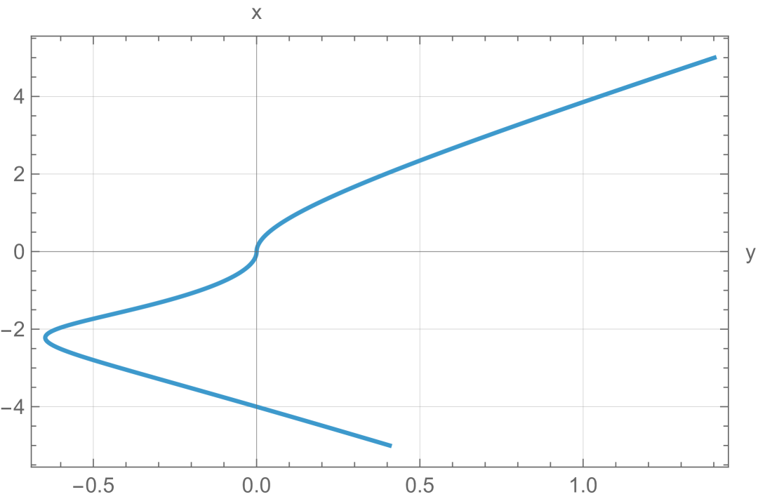
(a) The set ${\mathcal{R}}_{{\underline{\bm{k}}}}$ in case ${\underline{\bm{k}}}=(2,2)$

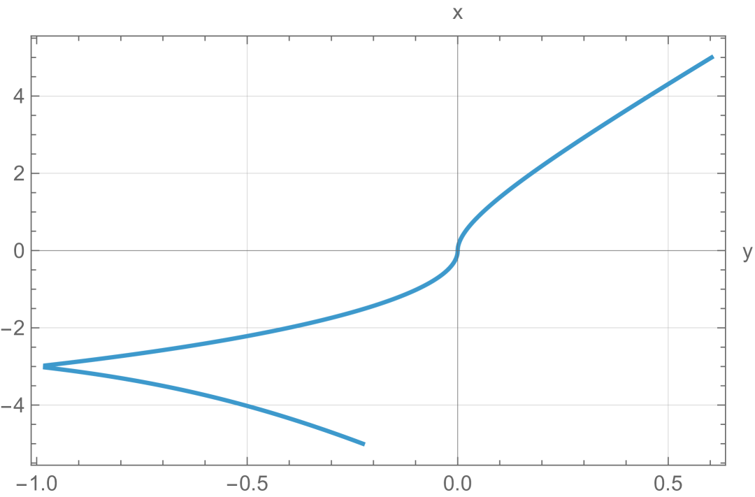
(b) The set ${\mathcal{R}}_{{\underline{\bm{k}}}}$ in case ${\underline{\bm{k}}}=(1,3)$

Remark 2.6.

Notice that in the regime of high Floquet parameter $y\rightarrow\pm\infty$ considered in Lemma 2.5, we have

$$\Omega({\underline{\bm{k}}}+\bm{\mu}) =\frac{\Omega({\underline{\bm{k}}})}{2}+\mathcal{O}\left(\frac{1}{y}\right),\quad\Omega(\bm{\mu})=\frac{\Omega({\underline{\bm{k}}})}{2}+\mathcal{O}\left(\frac{1}{y}\right),$$

so that, to leading order, the oscillation frequency of both secondary waves - corresponding to wavevectors ${\underline{\bm{k}}}+\bm{\mu}$ and $-\bm{\mu}$ - is approximately half that of the primary wave. This corresponds precisely to the regime of Parametric Subharmonic Instability (PSI), which is particularly relevant for inviscid fluids (see [23, Section 3.1]).

We shall now prove that, except for a discrete set, when $\bm{\mu}\in{\mathcal{R}}_{{\underline{\bm{k}}}}$ the double eigenvalue $\lambda^{-}_{\underline{\bm{k}}}(\bm{\mu})=\lambda^{+}_{\bm{0}}(\bm{\mu})$ has multiplicity exactly 2.

Proposition 2.7.

For any wavevector ${\underline{\bm{k}}}=({\mathtt{m}},{\mathtt{n}})^{T}\in{\mathbb{Z}}^{2}$ with ${\mathtt{m}},{\mathtt{n}}>0$, there exists a discrete set ${\mathcal{D}}_{\underline{\bm{k}}}\subset{\mathcal{R}}_{\underline{\bm{k}}}$ such that for any $\bm{\mu}\in{\mathcal{R}}_{\underline{\bm{k}}}\setminus{\mathcal{D}}_{\underline{\bm{k}}}$, there exists $\alpha=\alpha(\bm{\mu})>0$ such that:

(2.32) $$\inf_{\ell\in\mathbb{Z},\ell\neq 0}|w^{+}_{\ell{\underline{\bm{k}}}}(\bm{\mu})-w^{+}_{\bm{0}}(\bm{\mu})| \geq\alpha,\qquad\inf_{\ell\in\mathbb{Z},\ell\neq 1}|w^{-}_{\ell{\underline{\bm{k}}}}(\bm{\mu})-w^{-}_{\underline{\bm{k}}}(\bm{\mu})|\geq\alpha.$$

In particular, whenever $\bm{\mu}\in{\mathcal{R}}_{\underline{\bm{k}}}\setminus{\mathcal{D}}_{\underline{\bm{k}}}$, the operator ${\mathcal{L}}_{\bm{\mu},0}|_{H^{1}_{{\underline{\bm{k}}}}},$ has the isolated double eigenvalue $\lambda^{-}_{{\underline{\bm{k}}}}(\bm{\mu})=\lambda^{+}_{\bm{0}}(\bm{\mu})$.

Proof.

See Appendix B. ∎

By Proposition 2.7, for any $\bm{\mu}\in{\mathcal{R}}_{\underline{\bm{k}}}\setminus{\mathcal{D}}_{\underline{\bm{k}}}$, the spectrum of ${\mathcal{L}}_{\bm{\mu},0}|_{H^{1}_{{\underline{\bm{k}}}}}$ decomposes in two separated parts

(2.33) $$\sigma(\mathcal{L}_{\bm{\mu},0}|_{H^{1}_{{\underline{\bm{k}}}}}) =\sigma^{\prime}(\mathcal{L}_{\bm{\mu},0})\cup\sigma^{\prime\prime}(\mathcal{L}_{\bm{\mu},0}),\quad\sigma^{\prime}(\mathcal{L}_{\bm{\mu},0})\coloneqq\{\lambda^{+}\},\quad\lambda^{+}:=\lambda^{-}_{\underline{\bm{k}}}(\bm{\mu})\equiv\lambda^{+}_{\bm{0}}(\bm{\mu}).$$

With the notation of (2.23), we denote by $\mathcal{V}_{\underline{\bm{\mu}},0}$ the spectral subspace generated by the eigenvectors $\{f_{{\underline{\bm{k}}}}^{-},f_{\mathbf{0}}^{+}\}$ associated with the eigenvalue $\lambda^{+}$ in (2.26).

By Kato’s Similarity Transformation (Section 3, Lemma 3.1), we will show that whenever ${\epsilon}>0$ is small enough, the corresponding part of the spectrum of the linearized operator $\mathcal{L}_{\bm{\mu},\epsilon}$ remains isolated from the rest of $\sigma(\mathcal{L}_{\bm{\mu},\epsilon}|_{H^{1}_{{\underline{\bm{k}}}}})$ and takes the form

$$\lambda^{+}+\mathcal{O}(\epsilon).$$

Specifically, we will see that the spectrum of $\mathcal{L}_{\bm{\mu},\epsilon}|_{H^{1}_{{\underline{\bm{k}}}}}$ admits the decomposition

(2.34) $$\sigma\big{(}\mathcal{L}_{\bm{\mu},\epsilon}|_{H^{1}_{{\underline{\bm{k}}}}}\big{)}=\sigma^{\prime}\big{(}\mathcal{L}_{\bm{\mu},\epsilon}\big{)}\cup\sigma^{\prime\prime}\big{(}\mathcal{L}_{\bm{\mu},\epsilon}\big{)},$$

where $\sigma^{\prime}\big{(}\mathcal{L}_{\bm{\mu},\epsilon}\big{)}$ consists of two eigenvalues close to $\lambda^{+}$. Denoting by $\mathcal{V}_{\bm{\mu},\epsilon}$ the spectral subspace associated with $\sigma^{\prime}\big{(}\mathcal{L}_{\bm{\mu},\epsilon}\big{)}$, we provide the following matrix representation of the operator

$$\mathcal{L}_{\bm{\mu},\epsilon}\colon\mathcal{V}_{\bm{\mu},\epsilon}\to\mathcal{V}_{\bm{\mu},\epsilon}.$$

Theorem 2.

Let $\bm{\mu}\in{\mathcal{R}}_{\underline{\bm{k}}}\setminus{\mathcal{D}}_{\underline{\bm{k}}}$. There exists ${\epsilon}_{0}\equiv{\epsilon}_{0}(\bm{\mu})>0$ such that for any ${\epsilon}\in(0,{\epsilon}_{0})$, the operator ${\mathcal{L}}_{\bm{\mu},{\epsilon}}\colon{\mathcal{V}}_{\bm{\mu},{\epsilon}}\to{\mathcal{V}}_{\bm{\mu},{\epsilon}}$ is represented by the $2\times 2$ matrix:

(2.35) $$\begin{pmatrix}\lambda^{+}+{\rm i}\,r_{1}({\epsilon}^{2})&{\rm i}\,{\mathtt{b}}_{0}(\bm{\mu}){\epsilon}+{\rm i}\,r_{2}({\epsilon}^{2})\\ {\rm i}\,{\mathtt{b}}_{1}(\bm{\mu}){\epsilon}+{\rm i}r_{3}({\epsilon}^{2})&\lambda^{+}+{\rm i}\,r_{4}({\epsilon}^{2})\end{pmatrix}$$

where $\lambda^{+}$ is in (2.33) and

(2.36) $${\mathtt{b}}_{1}(\bm{\mu})=({\underline{\bm{k}}}^{\perp}\cdot{\bm{\mu}})\frac{\big{(}|{\underline{\bm{k}}}+{\bm{\mu}}|-|{\underline{\bm{k}}}|\big{)}\,(|{\underline{\bm{k}}}+{\bm{\mu}}|+|{\underline{\bm{k}}}|-|{\bm{\mu}}|\big{)}}{4N\,|{\underline{\bm{k}}}|\,|{\bm{\mu}}|\,|{\underline{\bm{k}}}+{\bm{\mu}}|},$$

$${\mathtt{b}}_{0}(\bm{\mu})=-({\underline{\bm{k}}}^{\perp}\cdot{\bm{\mu}})\frac{\big{(}|{\underline{\bm{k}}}|+|{\bm{\mu}}|\big{)}\,\big{(}|{\underline{\bm{k}}}+{\bm{\mu}}|+|{\underline{\bm{k}}}|-|{\bm{\mu}}|\big{)}}{4N\,|{\underline{\bm{k}}}|\,|{\bm{\mu}}|\,|{\underline{\bm{k}}}+{\bm{\mu}}|}.$$

Its eigenvalues are given by

(2.37) $$\lambda^{\pm}(\bm{\mu},{\epsilon})=\lambda^{+}+{\rm i}r({\epsilon}^{2})\pm{\epsilon}\sqrt{\mathtt{e}(\bm{\mu})+r({\epsilon})},$$

and

(2.38) $${\mathtt{e}}(\bm{\mu}) =-{\mathtt{b}}_{1}(\bm{\mu}){\mathtt{b}}_{0}(\bm{\mu})=({\underline{\bm{k}}}^{\perp}\cdot\bm{\mu})^{2}\,\frac{(|{\underline{\bm{k}}}+\bm{\mu}|-|{\underline{\bm{k}}}|)\,(|{\underline{\bm{k}}}|+|\bm{\mu}|)\,(|{\underline{\bm{k}}}+\bm{\mu}|+|{\underline{\bm{k}}}|-|\bm{\mu}|)^{2}}{16N^{2}\,|\bm{\mu}|^{2}\,|{\underline{\bm{k}}}+\bm{\mu}|^{2}\,|{\underline{\bm{k}}}|^{2}}.$$

In particular,

• in the regime of small Floquet parameter $|\bm{\mu}|\ll 1$, writing

  (2.39) $$\bm{\mu}(\tau)=\begin{cases}(\varphi_{+}({\mathtt{n}}\tau),{\mathtt{n}}\tau)^{T}&\mbox{ if }\tau>0\\ 0&\mbox{ if }\tau=0\\ (\varphi_{-}({\mathtt{n}}\tau),{\mathtt{n}}\tau)^{T}&\mbox{ if }\tau<0\end{cases}$$

  we have

  (2.40) $$\mathtt{e}(\bm{\mu}(\tau))=\frac{{\mathtt{m}}^{2}{\mathtt{n}}^{2}}{4N^{2}|{\underline{\bm{k}}}|^{2}}\tau+{\mathcal{O}}(\tau^{2})\ ,\quad\mbox{ as }\tau\to 0;$$

• in the regime of high Floquet parameter $|\bm{\mu}|\gg 1$, writing

  $$\bm{\mu}(\tau)=(\varphi_{+}(\tau),\tau)^{T}$$

  we have

  (2.41) $$\mathtt{e}(\bm{\mu}(\tau))=\frac{{\mathtt{m}}^{2}}{256N^{2}|{\underline{\bm{k}}}|^{6}}({\mathtt{n}}-\sqrt{3{\mathtt{m}}^{2}+4{\mathtt{n}}^{2}})^{2}(3{\mathtt{m}}^{2}+2{\mathtt{n}}^{2}+{\mathtt{n}}\sqrt{3{\mathtt{m}}^{2}+4{\mathtt{n}}^{2}})^{2}+\mathcal{O}(\tau^{-1}),\quad\mbox{ as }\tau\to\infty.$$

The proof is in Section 3.1.

3. Perturbative approach to separated eigenvalues

From now on, it is convenient to introduce the operator

(3.1) $${\mathscr{L}}_{\bm{\mu},{\epsilon}}:={\mathcal{L}}_{\bm{\mu},{\epsilon}}|_{H^{1}_{{\underline{\bm{k}}}}}\colon Y_{\underline{\bm{k}}}\to X_{\underline{\bm{k}}}$$

defined on the domain $Y_{\underline{\bm{k}}}\coloneqq H^{1}_{\underline{\bm{k}}}$ and taking values in $X_{\underline{\bm{k}}}\coloneqq H^{0}_{\underline{\bm{k}}}$. The property (2.34) states that the spectrum of ${\mathscr{L}}_{\bm{\mu},{\epsilon}}$ splits into two disjoint components. Following the approach in Kato’s Similarity Transformation (see [33] and Sec. 3 of [10]), we construct transformation operators which map isomorphically the unperturbed spectral subspace ${\mathcal{V}}_{\bm{\mu},0}$ - generated by the two eigenvectors associated with the double eigenvalue $\lambda^{+}$ - into the perturbed one ${\mathcal{V}}_{\bm{\mu},{\epsilon}}$.

Lemma 3.1.

Fix $\bm{\mu}\in\mathcal{R}_{{\underline{\bm{k}}}}\setminus{\mathcal{D}}_{{\underline{\bm{k}}}}$. Let $\Gamma$ be a closed, counterclockwise-oriented curve around $\lambda^{+}$ (see (2.33)) in the complex plane separating $\sigma^{\prime}({{\mathscr{L}}}_{{\bm{\mu}},0})=\{\lambda^{+}\}$ from the rest of the spectrum $\sigma^{\prime\prime}({{\mathscr{L}}}_{\bm{\mu},0})$ in (2.33). Then there exists ${\epsilon}_{0}\equiv{\epsilon}_{0}(\bm{\mu})>0$ such that, for any ${\epsilon}\in(0,{\epsilon}_{0})$, the following statements hold true:

1. the curve $\Gamma$ belongs to the resolvent set of the operator ${\mathscr{L}}_{\bm{\mu},\epsilon}:Y_{\underline{\bm{k}}}\to X_{\underline{\bm{k}}}$ in (3.1) ;

2. the operators

   (3.2) $$P_{\bm{\mu},\epsilon} \coloneqq-\frac{1}{2\pi\mathrm{i}}\oint_{\Gamma}({{\mathscr{L}}}_{\bm{\mu},\epsilon}-\lambda)^{-1}\mathrm{d}\lambda:X_{\underline{\bm{k}}}\to Y_{\underline{\bm{k}}}$$

   are well-defined projectors commuting with ${{\mathscr{L}}}_{\bm{\mu},\epsilon}$, namely

   (3.3) $$P_{\bm{\mu},\epsilon}^{2}=P_{\bm{\mu},\epsilon},\;\;P_{\bm{\mu},\epsilon}{{\mathscr{L}}}_{\bm{\mu},\epsilon}=\mathcal{{\mathscr{L}}}_{\bm{\mu},\epsilon}P_{\bm{\mu},\epsilon},$$

   the map $\epsilon\mapsto P_{\bm{\mu},\epsilon}$ is analytic from $B(\epsilon_{0})$ to $L(X_{\underline{\bm{k}}},Y_{\underline{\bm{k}}})$ and the projectors are reversibility preserving, i.e. $\overline{\rho}P_{\bm{\mu},{\epsilon}}=P_{\bm{\mu},{\epsilon}}\overline{\rho}$;

3. the domain $Y_{\underline{\bm{k}}}$ of the operator ${{\mathscr{L}}}_{\bm{\mu},\epsilon}$ decomposes as the direct sum

   (3.4) $$Y_{\underline{\bm{k}}} =\mathrm{Ker}(P_{\bm{\mu},\epsilon})\oplus\mathcal{V}_{\bm{\mu},\epsilon},\;\;\mathcal{V}_{\bm{\mu},\epsilon}\coloneqq\mathrm{Rg}(P_{\bm{\mu},\epsilon})=\mathrm{Ker}(\mathrm{id}-P_{\bm{\mu},\epsilon}),$$

   where the closed subspaces $\mathrm{Ker}(P_{\bm{\mu},\epsilon})$ and $\mathcal{V}_{\bm{\mu},\epsilon}$ are invariant under ${{\mathscr{L}}}_{\bm{\mu},\epsilon}$,

   $${{\mathscr{L}}}_{\bm{\mu},\epsilon}:\mathcal{V}_{\bm{\mu},\epsilon}\to\mathcal{V}_{\bm{\mu},\epsilon},\;\;{{\mathscr{L}}}_{\bm{\mu},\epsilon}:\mathrm{Ker}(\mathcal{P}_{\bm{\mu},\epsilon})\to\mathrm{Ker}(\mathcal{P}_{\bm{\mu},\epsilon}).$$

   Moreover,

   $$\sigma({{\mathscr{L}}}_{\bm{\mu},\epsilon})\cap\{z\in\mathbb{C}\;\;\text{inside}\;\;\Gamma\} =\sigma({{\mathscr{L}}}_{\bm{\mu},\epsilon}|_{\mathcal{V}_{\bm{\mu},\epsilon}})=\sigma^{\prime}({{\mathscr{L}}}_{\bm{\mu},\epsilon}),$$

   (3.5) $$\sigma({{\mathscr{L}}}_{\bm{\mu},\epsilon})\cap\{z\in\mathbb{C}\;\;\text{outside}\;\;\Gamma\} =\sigma({{\mathscr{L}}}_{\bm{\mu},\epsilon}|_{\mathrm{Ker}({P}_{\bm{\mu},\epsilon})})=\sigma^{\prime\prime}({{\mathscr{L}}}_{\bm{\mu},\epsilon}),$$

   proving the “semicontinuity property” (2.34) of separated parts of the spectrum;

4. the subspaces $\mathcal{V}_{\bm{\mu},\epsilon}$ are isomorphic one to another. In particular, $\mathrm{dim}(\mathcal{V}_{\bm{\mu},\epsilon})=\mathrm{dim}(\mathcal{V}_{{\bm{\mu}},0})=2$ for all $\epsilon\in B(\epsilon_{0})$.

By Lemma 3.1 we ensure that the corresponding perturbed eigenvalues remain isolated from the rest of the spectrum. We now consider the following basis for the perturbed spectral subspace $\mathcal{V}_{{\bm{\mu}},\epsilon}$:

(3.6) $$\mathcal{F} \coloneqq\{f_{{\underline{\bm{k}}}}^{-}(\bm{\mu},\epsilon),f_{\bm{0}}^{+}(\bm{\mu},\epsilon)\},\quad f_{\bm{j}}^{\sigma}(\bm{\mu},\epsilon)\coloneqq P_{\bm{\mu},\epsilon}f_{\bm{j}}^{\sigma}(\bm{\mu}),\;\bm{j}={\underline{\bm{k}}},\bm{0},$$

given by the projection $P_{\bm{\mu},\epsilon}$ in (3.2) of $f_{{\underline{\bm{k}}}}^{-}(\bm{\mu}),f_{\bm{0}}^{+}(\bm{\mu})$ in (2.23) (forming a basis of $\mathcal{V}_{{\bm{\mu}},0}$).

Below, we compute the $2\times 2$ matrix representing the action of the operator ${{\mathscr{L}}}_{\bm{\mu},\epsilon}:\mathcal{V}_{\bm{\mu},\epsilon}\to\mathcal{V}_{\bm{\mu},\epsilon}$ on the basis ${\mathcal{F}}$.

Lemma 3.2.

Fix $\bm{\mu}\in\mathcal{R}_{{\underline{\bm{k}}}}\setminus{\mathcal{D}}_{{\underline{\bm{k}}}}$. The operator ${{\mathscr{L}}}_{\bm{\mu},\epsilon}:\mathcal{V}_{\bm{\mu},\epsilon}\to\mathcal{V}_{\bm{\mu},\epsilon}$ on the basis $\mathcal{F}$ in (3.6) admits the following matrix representation:

(3.7) $${\mathtt{L}}({\bm{\mu},{\epsilon}}) ={\mathtt{I}}({\bm{\mu},{\epsilon}})^{-1}{\mathtt{A}}({\bm{\mu},{\epsilon}}),$$

where

(3.8) $${\mathtt{I}}({\bm{\mu},{\epsilon}}):=\begin{pmatrix}\langle\mathfrak{I}(\bm{\mu},\epsilon)f_{{\underline{\bm{k}}}}^{-},f_{{\underline{\bm{k}}}}^{-}\rangle&\langle\mathfrak{I}(\bm{\mu},\epsilon)f_{\bm{0}}^{+},f_{{\underline{\bm{k}}}}^{-}\rangle\\ \langle\mathfrak{I}(\bm{\mu},\epsilon)f_{{\underline{\bm{k}}}}^{-},f_{\bm{0}}^{+}\rangle&\langle\mathfrak{I}(\bm{\mu},\epsilon)f_{\bm{0}}^{+},f_{\bm{0}}^{+}\rangle\end{pmatrix}=\begin{pmatrix}\iota_{11}(\bm{\mu},\epsilon)&\iota_{01}(\bm{\mu},\epsilon)\\ \iota_{01}(\bm{\mu},\epsilon)&\iota_{00}(\bm{\mu},\epsilon)\end{pmatrix}\ ,$$

(3.9) $${\mathtt{A}}({\bm{\mu},{\epsilon}}):=\begin{pmatrix}\langle\mathfrak{L}({\bm{\mu},\epsilon})f_{{\underline{\bm{k}}}}^{-},f_{{\underline{\bm{k}}}}^{-}\rangle&\langle\mathfrak{L}({\bm{\mu},\epsilon})f_{\bm{0}}^{+},f_{{\underline{\bm{k}}}}^{-}\rangle\\ \langle\mathfrak{L}({\bm{\mu},\epsilon})f_{{\underline{\bm{k}}}}^{-},f_{\bm{0}}^{+}\rangle&\langle\mathfrak{L}({\bm{\mu},\epsilon})f_{\bm{0}}^{+},f_{\bm{0}}^{+}\rangle\end{pmatrix}={\rm i}\begin{pmatrix}a_{11}(\bm{\mu},\epsilon)&a_{01}(\bm{\mu},\epsilon)\\ a_{10}(\bm{\mu},\epsilon)&a_{00}(\bm{\mu},\epsilon)\end{pmatrix}$$

and $f_{{\underline{\bm{k}}}}^{-}\equiv f_{{\underline{\bm{k}}}}^{-}(\bm{\mu}),f_{\bm{0}}^{+}\equiv f_{\bm{0}}^{+}(\bm{\mu})$ in (2.23), and

(3.10) $$\mathfrak{I}(\bm{\mu},{\epsilon}):=P_{\bm{\mu},0}^{*}\,P_{\bm{\mu},{\epsilon}}^{*}\,P_{\bm{\mu},{\epsilon}}\,P_{\bm{\mu},0}\ ,\qquad\mathfrak{L}(\bm{\mu},{\epsilon}):=P_{\bm{\mu},0}^{*}\,P_{\bm{\mu},{\epsilon}}^{*}\,{\mathscr{L}}_{\bm{\mu},{\epsilon}}\,P_{\bm{\mu},{\epsilon}}P_{\bm{\mu},0}\ .$$

The functions ${\epsilon}\to\iota_{ij}(\bm{\mu},{\epsilon})$ and ${\epsilon}\to a_{ij}(\bm{\mu},{\epsilon})$ are real valued and analytic. Furthermore

(3.11) $${\mathtt{I}}(\bm{\mu},0)=\begin{pmatrix}\iota_{11}(\bm{\mu},0)&0\\ 0&\iota_{00}(\bm{\mu},0)\end{pmatrix}\ ,\qquad{\mathtt{A}}(\bm{\mu},0)=\begin{pmatrix}\lambda_{\underline{\bm{k}}}^{-}(\bm{\mu})\,\iota_{11}(\bm{\mu},0)&0\\ 0&\lambda_{\bm{0}}^{+}(\bm{\mu})\,\iota_{00}(\bm{\mu},0)\end{pmatrix},$$

and

(3.12) $$\iota_{11}(\bm{\mu},0) =\langle f_{{\underline{\bm{k}}}}^{-},f_{{\underline{\bm{k}}}}^{-}\rangle\,=\,\frac{1}{2}\left(N^{2}+|{\underline{\bm{k}}}+\underline{\bm{\mu}}|^{2}\right),\quad\iota_{00}(\bm{\mu},0) =\langle f_{\bm{0}}^{+},f_{\bm{0}}^{+}\rangle\,=\,\frac{1}{2}\left(N^{2}+|\underline{\bm{\mu}}|^{2}\right).$$

Proof.

We write

$$\mathcal{L}_{\bm{\mu},\epsilon}f_{{\underline{\bm{k}}}}^{-}(\bm{\mu},{\epsilon})=\alpha f_{{\underline{\bm{k}}}}^{-}(\bm{\mu},{\epsilon})+\beta f_{\bm{0}}^{+}(\bm{\mu},{\epsilon}), \;\;\;\;\mathcal{L}_{\bm{\mu},\epsilon}f_{\bm{0}}^{+}(\bm{\mu},{\epsilon})=\gamma f_{{\underline{\bm{k}}}}^{-}(\bm{\mu},{\epsilon})+\delta f_{\bm{0}}^{+}(\bm{\mu},{\epsilon}),$$

for some $\alpha,\beta,\gamma,\delta\in\mathbb{C}$. Taking the scalar product with $f_{{\underline{\bm{k}}}}^{-}(\bm{\mu},{\epsilon})$, $f_{0}^{+}(\bm{\mu},{\epsilon})$ and using (3.6) give (3.7) (3.8) and (3.9).

The reality of the entries of ${\mathtt{I}}(\bm{\mu},{\epsilon})$ and the purely imaginary nature of ${\mathtt{A}}(\bm{\mu},{\epsilon})$ follow from the reversibility property (2.25), the reversibility of the projector $P_{\bm{\mu},{\epsilon}}$ (Lemma 3.1, point 2), the complex reversibility of ${\mathscr{L}}_{\bm{\mu},{\epsilon}}$ (see (2.12)), and the identity

(3.13) $$(f,g)=\overline{(\overline{\varrho}f,\overline{\varrho}g)}\ ,\quad\forall f,g\in L^{2}({\mathbb{R}}^{2},{\mathbb{C}})\ .$$

∎

In the following, we provide an asymptotic expansion of the entries of ${\mathtt{L}}(\bm{\mu},{\epsilon})$.

Proposition 3.3.

Fix $\bm{\mu}\in\mathcal{R}_{{\underline{\bm{k}}}}\setminus{\mathcal{D}}_{{\underline{\bm{k}}}}$. The real analytic entries of the matrix ${\mathtt{L}}(\bm{\mu},{\epsilon})$ in (3.7) admit the following expansions as ${\epsilon}\to 0$:

(3.14) $$\iota_{11}(\bm{\mu},{\epsilon}) =\iota_{11}(\bm{\mu},0)+\mathcal{O}({\epsilon}^{2}),\quad\iota_{10}(\bm{\mu},{\epsilon})=\gamma_{1}(\bm{\mu}){\epsilon}+\mathcal{O}({\epsilon}^{2}),\quad\iota_{00}(\bm{\mu},{\epsilon})=\iota_{00}(\bm{\mu},0)+\mathcal{O}({\epsilon}^{2}),$$

(3.15) $$a_{11}(\bm{\mu},{\epsilon}) =\underline{w}\,\iota_{11}(\bm{\mu},0)+\mathcal{O}({\epsilon}^{2})\ ,\quad a_{00}(\bm{\mu},{\epsilon})=\underline{w}\,\iota_{00}(\bm{\mu},0)+\mathcal{O}({\epsilon}^{2}),\$$

(3.16) $$a_{10}(\bm{\mu},{\epsilon}) =\beta_{1}(\bm{\mu}){\epsilon}+\mathcal{O}({\epsilon}^{2})\ ,\quad a_{01}(\bm{\mu},{\epsilon})=\beta_{0}(\bm{\mu}){\epsilon}+\mathcal{O}({\epsilon}^{2})\ .$$

where $\iota_{11}(\bm{\mu},0)$ and $\iota_{00}(\bm{\mu},0)$ are given in (3.12),

(3.17) $${\underline{w}}:={\underline{w}}(\bm{\mu}):=-{\rm i}\lambda^{+}=\underline{\bm{c}}\cdot\bm{\mu}+\Omega(\bm{\mu})=\underline{\bm{c}}\cdot({\underline{\bm{k}}}+\bm{\mu})-\Omega({\underline{\bm{k}}}+\bm{\mu})$$

with $\underline{\bm{c}}$ in (2.2), and finally the functions $\beta_{1}(\bm{\mu}),\beta_{0}(\bm{\mu})$ and $\gamma_{1}(\bm{\mu})$ fulfill

(3.18) $$\beta_{1}(\bm{\mu})-\gamma_{1}(\bm{\mu}){\underline{w}}(\bm{\mu}) =\frac{{\epsilon}}{8}({\underline{\bm{k}}}^{\perp}\cdot{\bm{\mu}})\frac{\big{(}|{\underline{\bm{k}}}+{\bm{\mu}}|-|{\underline{\bm{k}}}|\big{)}\,(|{\underline{\bm{k}}}+{\bm{\mu}}|+|{\underline{\bm{k}}}|-|{\bm{\mu}}|\big{)}\,\big{(}N^{2}+|{\bm{\mu}}|^{2}\big{)}}{N\,|{\underline{\bm{k}}}|\,|{\bm{\mu}}|\,|{\underline{\bm{k}}}+{\bm{\mu}}|}$$

(3.19) $$\beta_{0}(\bm{\mu})-\gamma_{1}(\bm{\mu}){\underline{w}}(\bm{\mu}) =-\frac{{\epsilon}}{8}({\underline{\bm{k}}}^{\perp}\cdot{\bm{\mu}})\frac{\big{(}|{\underline{\bm{k}}}|+|{\bm{\mu}}|\big{)}\,\big{(}|{\underline{\bm{k}}}+{\bm{\mu}}|+|{\underline{\bm{k}}}|-|{\bm{\mu}}|\big{)}\,\big{(}|{\underline{\bm{k}}}+{\bm{\mu}}|^{2}+N^{2}\big{)}}{N\,|{\underline{\bm{k}}}|\,|{\bm{\mu}}|\,|{\underline{\bm{k}}}+{\bm{\mu}}|}$$

The proof of Proposition 3.3 relies on machinery introduced in the next section, with the proof itself deferred to Section 5. Meanwhile, assuming Proposition 3.3, we can prove Theorem 2.

3.1. Proof of Theorem 2

By (3.7) and the expansions of Proposition 3.3,

(3.20) $${\mathtt{L}}(\bm{\mu},{\epsilon})=\begin{pmatrix}\lambda^{+}+{\rm i}r_{1}({\epsilon}^{2})&{\rm i}\dfrac{\beta_{0}(\bm{\mu})-\gamma_{1}(\bm{\mu})\underline{w}(\bm{\mu})}{\iota_{11}(\bm{\mu},0)}{\epsilon}+{\rm i}r_{2}({\epsilon}^{2})\\ {\rm i}\dfrac{\beta_{1}(\bm{\mu})-\gamma_{1}(\bm{\mu})\underline{w}(\bm{\mu})}{\iota_{00}(\bm{\mu},0)}{\epsilon}+{\rm i}r_{3}({\epsilon}^{2})&\lambda^{+}+{\rm i}r_{4}({\epsilon}^{2})\end{pmatrix}$$

Next, ${\mathtt{b}}_{1}(\bm{\mu}):=\frac{\beta_{1}(\bm{\mu})-\gamma_{1}(\bm{\mu})\underline{w}(\bm{\mu})}{\iota_{00}(\bm{\mu},0)}$ is obtained by (3.18) and (3.12). Similarly ${\mathtt{b}}_{0}(\bm{\mu}):=\frac{\beta_{0}(\bm{\mu})-\gamma_{1}(\bm{\mu})\underline{w}(\bm{\mu})}{\iota_{11}(\bm{\mu},0)}$ is computed via (3.19) and (3.12). The eigenvalues (2.37) are readily computed.

The asymptotics in (2.40) and (2.41) are obtained by computing ${\mathtt{e}}(\bm{\mu})$ along the corresponding parametrizations, using the asymptotics of the functions $\varphi_{\pm}$ in Lemma 2.5.

4. Taylor expansion of the operators and entanglement coefficients

This section introduces the technical machinery to prove Proposition 3.3, providing the entanglement coefficients (4.18). To begin with, we introduce the jets of the operator ${\mathscr{L}}_{\bm{\mu},{\epsilon}}$ in (3.1), obtained by Taylor-expanding the operator ${\mathscr{L}}_{\bm{\mu},{\epsilon}}$ at the point $(\bm{\mu},0)$:

(4.1) $${\mathscr{L}}_{j}:=\frac{1}{j!}\big{(}\partial^{j}_{\epsilon}{\mathscr{L}}_{\bm{\mu},{\epsilon}}\big{)}(\bm{\mu},0)\,{\epsilon}^{j}\,\ ,\qquad j\in{\mathbb{N}}_{0}\ ,$$

so that

(4.2) $${\mathscr{L}}_{\bm{\mu},{\epsilon}}={\mathscr{L}}_{0}+{\mathscr{L}}_{1}+{\mathcal{O}}_{2}\,.$$

Explicitly, by (3.1), (2.11) and (2.2) we have that ${\mathscr{L}}_{0}$ is the matrix of Fourier multipliers

(4.3) $${\mathscr{L}}_{0}=\begin{pmatrix}\underline{\bm{c}}\cdot(\nabla+{\rm i}\bm{\mu})&-N^{2}\,(\partial_{x}+{\rm i}\mu_{1})\,\left|\nabla+{\rm i}\bm{\mu}\right|^{-2}\\ -(\partial_{x}+{\rm i}\mu_{1})&\underline{\bm{c}}\cdot(\nabla+{\rm i}\bm{\mu})\end{pmatrix}$$

whereas ${\mathscr{L}}_{1}$ is the operator

(4.4) $${\mathscr{L}}_{1}={\epsilon}\cos({\underline{\bm{k}}}\cdot\bm{x})\begin{pmatrix}-(N\,|{\underline{\bm{k}}}|)^{-1}\,{\underline{\bm{k}}}^{\perp}\cdot(\nabla+{\rm i}\bm{\mu})&-{\underline{\bm{k}}}\cdot(\operatorname{\nabla^{\perp}}+{\rm i}\bm{\mu}^{\perp})\,|{\bf D+\bm{\mu}}|^{-2}\\ 0&-(N\,|{\underline{\bm{k}}}|)^{-1}\,{\underline{\bm{k}}}^{\perp}\cdot(\nabla+{\rm i}\bm{\mu})-N^{-1}\,|{\underline{\bm{k}}}|\,{\underline{\bm{k}}}\cdot(\operatorname{\nabla^{\perp}}+{\rm i}\bm{\mu}^{\perp})|{\bf D}+\bm{\mu}|^{-2}\end{pmatrix}\ .$$

Analogously we Taylor-expand the projectors $P_{\bm{\mu},{\epsilon}}$ in (3.2) at the point $(\bm{\mu},0)$ as

$$P_{\bm{\mu},{\epsilon}}=P_{0}+P_{1}+{\mathcal{O}}_{2}\,$$

where

(4.5) $$P_{0}=P_{\bm{\mu},0}=-\frac{1}{2\pi{\rm i}}\oint_{\Gamma}({\mathscr{L}}_{\bm{\mu},0}-\lambda)^{-1}{\rm d}\lambda\ ,$$

and

(4.6) $$P_{1}=\mathcal{P}\big{[}{\mathscr{L}}_{1}\big{]}\ ,\quad\mathcal{P} \big{[}A\big{]}=\frac{1}{2\pi{\rm i}}\oint_{\Gamma}({\mathscr{L}}_{\bm{\mu},0}-\lambda)^{-1}\,A\,({\mathscr{L}}_{\bm{\mu},0}-\lambda)^{-1}{\rm d}\lambda\,,$$

where $\Gamma$ is the curve of Lemma 3.1.

We therefore obtain the following lemma about the jets of the operators $\mathfrak{L}({\bm{\mu},{\epsilon}})$ and $\mathfrak{I}(\bm{\mu},{\epsilon})$:

Lemma 4.1.

The operators $\mathfrak{L}(\bm{\mu},{\epsilon})$ and $\mathfrak{I}(\bm{\mu},{\epsilon})$ in (3.10) have the Taylor expansions

(4.7) $$\mathfrak{L}({\bm{\mu},{\epsilon}})=\mathfrak{L}_{0}+\mathfrak{L}_{1}+{\mathcal{O}}_{2}\ ,\qquad\mathfrak{I}({\bm{\mu},{\epsilon}})=\mathfrak{I}_{0}+\mathfrak{I}_{1}+{\mathcal{O}}_{2}$$

where

(4.8a) $$\mathfrak{L}_{0} :=P_{0}^{*}{{\mathscr{L}}}_{0}P_{0}\,,\quad\mathfrak{L}_{1}:=P_{0}^{*}\left(P_{1}^{*}{\mathscr{L}}_{0}+{\mathscr{L}}_{0}P_{1}+{{\mathscr{L}}}_{1}\right)P_{0}\,,$$

(4.8b) $$\mathfrak{I}_{0} :=P_{0}^{*}P_{0}\,,\quad\mathfrak{I}_{1}:=P_{0}^{*}(P_{1}+P_{1}^{*})P_{0}\,,$$

with ${{\mathscr{L}}}_{j}$, $j=0,1$, in (4.3), (4.4) and $P_{j}$, $j=0,1$, in (4.5).

Proof.

This readily follows Taylor-expanding the explicit formula (3.10), using the fact that $P_{j}^{2}=P_{j}$. ∎

4.1. Entanglement coefficients.

Next we introduce the entanglement coefficients, that describe the action of the jets ${\mathscr{L}}_{\ell}$ and ${\mathcal{J}}(\mu){\mathscr{L}}_{\ell}$ over the vectors $\{f_{\bm{k}}^{\sigma}\}_{\bm{k}\in{\mathbb{Z}}^{2},\sigma=\pm}$, $f_{\bm{k}}^{\sigma}:=f_{\bm{k}}^{\sigma}(\bm{\mu})$ in (2.23), forming a basis of $L^{2}({\mathbb{T}}^{2},{\mathbb{C}}^{2})$ and fulfilling the symplectic relation (2.24).

First, given a linear operator $A=\begin{pmatrix}A_{1}&A_{2}\\ A_{3}&A_{4}\end{pmatrix}\colon H^{1}_{{\underline{\bm{k}}}}\to H^{0}_{{\underline{\bm{k}}}}$ (recall definition (2.8)) we define for any $j_{1},j_{2}\in{\mathbb{Z}}$ its matrix elements

(4.9) $$A^{j_{1}}_{j_{2}}:=\begin{pmatrix}(A_{1}[e^{{\rm i}j_{1}{\underline{\bm{k}}}\cdot\bm{x}}],\ e^{{\rm i}j_{2}{\underline{\bm{k}}}\cdot\bm{x}})_{L^{2}({\mathbb{T}}^{2})}&(A_{2}[e^{{\rm i}j_{1}{\underline{\bm{k}}}\cdot\bm{x}}],\ e^{{\rm i}j_{2}{\underline{\bm{k}}}\cdot\bm{x}})_{L^{2}({\mathbb{T}}^{2})}\\ (A_{3}[e^{{\rm i}j_{1}{\underline{\bm{k}}}\cdot\bm{x}}],\ e^{{\rm i}j_{2}{\underline{\bm{k}}}\cdot\bm{x}})_{L^{2}({\mathbb{T}}^{2})}&(A_{4}[e^{{\rm i}j_{1}{\underline{\bm{k}}}\cdot\bm{x}}],\ e^{{\rm i}j_{2}{\underline{\bm{k}}}\cdot\bm{x}})_{L^{2}({\mathbb{T}}^{2})}\end{pmatrix}\ ,$$

where for $f,g\in L^{2}({\mathbb{T}}^{2},{\mathbb{C}})$ we denoted

$$(f,g)=\frac{1}{(2\pi)^{2}}\int_{{\mathbb{T}}^{2}}f(\bm{x})\,\overline{g(\bm{x})}\,d\bm{x}\ .$$

In this way the action of $A\colon H^{1}_{{\underline{\bm{k}}}}\to H^{0}_{{\underline{\bm{k}}}}$ is given by

$$H^{1}_{{\underline{\bm{k}}}}\ni\vec{h}(\bm{x})=\sum_{j_{1}\in{\mathbb{Z}}}\vec{h}_{j_{1}}e^{{\rm i}j_{1}{\underline{\bm{k}}}\cdot\bm{x}}\mapsto(A\vec{h})(\bm{x})=\sum_{j_{2}\in{\mathbb{Z}}}\Big{(}\sum_{j_{1}\in{\mathbb{Z}}}A^{j_{1}}_{j_{2}}\,\vec{h}_{j_{1}}\Big{)}\,e^{{\rm i}j_{2}{\underline{\bm{k}}}\cdot\bm{x}}\in H^{0}_{{\underline{\bm{k}}}}\,.$$

Next, given $\bm{\kappa}\in{\underline{\bm{k}}}{\mathbb{Z}}$, we define the projected operator $A^{[\bm{\kappa}]}$ whose matrix coefficients are those of $A$ supported on the “band” $(j_{2}-j_{1}){\underline{\bm{k}}}=\bm{\kappa}$, i.e.

(4.10) $$A^{[\bm{\kappa}]}\vec{h}=\sum_{j_{1},j_{2}\in{\mathbb{Z}}\atop(j_{2}-j_{1}){\underline{\bm{k}}}=\bm{\kappa}}A^{j_{1}}_{j_{2}}\,\vec{h}_{j_{1}}\,e^{{\rm i}j_{2}{\underline{\bm{k}}}\cdot x}\,.$$

The following identities, for operators $H^{\infty}_{\underline{\bm{k}}}\to H^{\infty}_{\underline{\bm{k}}}$ are easy to check:

(4.11) $$A=\sum_{\bm{\kappa}\in{\underline{\bm{k}}}{\mathbb{Z}}}A^{[\bm{\kappa}]}\ ,\qquad\big{[}A^{[\bm{\kappa}]}\big{]}^{*}=(A^{*})^{[-\bm{\kappa}]}\ ,\qquad(A\circ B)^{[\bm{\kappa}]}=\sum_{\bm{\kappa}_{1},\bm{\kappa}_{2}\in{\underline{\bm{k}}}{\mathbb{Z}}\atop\bm{\kappa}_{1}+\bm{\kappa}_{2}=\bm{\kappa}}A^{[\bm{\kappa}_{1}]}\circ B^{[\bm{\kappa}_{2}]}\ .$$

Following [9], we introduce the spaces $\mathfrak{F}_{\ell}$, which highlight important structural properties of the jets of the operator $\mathcal{L}_{\bm{\mu},{\epsilon}}$. Roughly speaking, these are spaces of operators whose jets $A_{j}$ have “bands” of order at most $j$ and share the same parity as $j$.

Definition 4.2 (Spaces $\mathfrak{F}_{\ell}$).

For any $\ell\in\mathbb{N}_{0}$, we define $\mathfrak{F}_{\ell}$ as the space of operators $H^{\infty}_{{\underline{\bm{k}}}}\to H^{\infty}_{{\underline{\bm{k}}}}$ satisfying

(4.12) $$A^{[n{\underline{\bm{k}}}]}=0\quad\text{if }|n|>\ell\quad\text{or}\quad n\not\equiv\ell\pmod{2}\,.$$

The following lemma, proved as in [9, Lemma 5.5], states some properties of the spaces $\mathfrak{F}_{\ell}$ which will be used repeatedly.

Lemma 4.3.

Let $A\in\mathfrak{F}_{\ell}$, $B\in\mathfrak{F}_{\ell^{\prime}}$. Then

• Composition: $A\circ B\in\mathfrak{F}_{\ell+\ell^{\prime}}$ with $(A\circ B)^{[\pm(\ell+\ell^{\prime}){\underline{\bm{k}}}]}=A^{[\pm\ell{\underline{\bm{k}}}]}\circ B^{[\pm\ell^{\prime}{\underline{\bm{k}}}]}$;

• Adjoint: $A^{*}\in\mathfrak{F}_{\ell}$.

• Finite range interactions: For any $\vec{v}_{1},\vec{v}_{2}\in{\mathbb{C}}^{2}$,

  (4.13) $$(A\,\vec{v}_{1}e^{{\rm i}j_{1}{\underline{\bm{k}}}\cdot\bm{x}},\vec{v}_{2}e^{{\rm i}j_{2}{\underline{\bm{k}}}\cdot\bm{x}})=0\ \ \mbox{ if }|j_{1}-j_{2}|>\ell\mbox{ or }j_{1}-j_{2}\not\equiv\ell\mbox{ mod }2\ .$$

Proof.

(i) It follows from the third of (4.11), using that if $\bm{\kappa}=n{\underline{\bm{k}}}$, $\bm{\kappa}_{1}=j_{1}{\underline{\bm{k}}}$, $\bm{\kappa}_{2}=j_{2}{\underline{\bm{k}}}$, then necessarily $j_{1}\equiv\ell\mod 2$, $j_{2}\equiv\ell^{\prime}\mod 2$, hence $j_{1}+j_{2}\equiv\ell+\ell^{\prime}\mod 2$, and if $\ell+\ell^{\prime}<|n|\leq|j_{1}|+|j_{2}|$, then either $|j_{1}|>\ell$ hence $A^{[\bm{\kappa}_{1}]}=0$, or $|j_{2}|>\ell^{\prime}$ hence $B^{[\bm{\kappa}_{2}]}=0$. Moreover, if $|n|=\ell+\ell^{\prime}$, being $j_{1}+j_{2}=n$ and $|j_{1}|\leq\ell$, $|j_{2}|\leq\ell^{\prime}$, the only possibility is that $j_{1}=\ell$, $j_{2}=\ell^{\prime}$.
(ii) It follows from the second of (4.11).
(iii) By the first of (4.11) and the definition (4.10), we have

$$(A\,\vec{v}_{1}e^{{\rm i}j_{1}{\underline{\bm{k}}}\cdot\bm{x}},\vec{v}_{2}e^{{\rm i}j_{2}{\underline{\bm{k}}}\cdot\bm{x}})=\sum_{\bm{\kappa}\in{\underline{\bm{k}}}{\mathbb{Z}}}(A^{[\bm{\kappa}]}\,\vec{v}_{1}e^{{\rm i}j_{1}{\underline{\bm{k}}}\cdot\bm{x}},\vec{v}_{2}e^{{\rm i}j_{2}{\underline{\bm{k}}}\cdot\bm{x}})=(A^{[(j_{2}-j_{1}){\underline{\bm{k}}}]}\,\vec{v}_{1}e^{{\rm i}j_{1}{\underline{\bm{k}}}\cdot\bm{x}},\vec{v}_{2}e^{{\rm i}j_{2}{\underline{\bm{k}}}\cdot\bm{x}})$$

and the claim follows from property (4.12). ∎

In the next lemma, we state useful properties of the jets of the operators ${\mathscr{L}}_{\bm{\mu},{\epsilon}}$, $P_{\bm{\mu},{\epsilon}}$, $\mathfrak{L}(\bm{\mu},{\epsilon})$, $\mathfrak{J}(\bm{\mu},{\epsilon})$.

Lemma 4.4.

The jets of the operators ${\mathscr{L}}_{\bm{\mu},{\epsilon}}$ in (3.1), $P_{\bm{\mu},{\epsilon}}$ in (3.2), $\mathfrak{L}(\bm{\mu},{\epsilon})$ and $\mathfrak{J}(\bm{\mu},{\epsilon})$ in (3.10) fulfill:

(4.14) $${\mathscr{L}}_{\ell}\ ,\ \ P_{\ell}\ ,\ \ \mathfrak{L}_{\ell}\ ,\ \ \mathfrak{I}_{\ell}\in\mathfrak{F}_{\ell}\ ,\qquad\ell=0,1\ .$$

In addition ${\mathscr{L}}_{0}^{[\bm{0}]}={\mathscr{L}}_{0}$, the $\pm{\underline{\bm{k}}}$-th band of the operator ${\mathscr{L}}_{1}$ in (4.4) is

(4.15) $${\mathscr{L}}_{1}^{[\pm{\underline{\bm{k}}}]} =\frac{{\epsilon}}{2}e^{\pm{\rm i}{\underline{\bm{k}}}\cdot\bm{x}}\,\begin{pmatrix}-(N\,|{\underline{\bm{k}}}|)^{-1}\,{\rm i}{\underline{\bm{k}}}^{\perp}\cdot\bm{\mu}&{\rm i}{\underline{\bm{k}}}^{\perp}\cdot\bm{\mu}\,|\bm{D}+\bm{\mu}|^{-2}\\ 0&-(N\,|{\underline{\bm{k}}}|)^{-1}\,{\rm i}{\underline{\bm{k}}}^{\perp}\cdot\bm{\mu}+N^{-1}\,|{\underline{\bm{k}}}|\,{\rm i}{\underline{\bm{k}}}^{\perp}\cdot\bm{\mu}|\bm{D}+\bm{\mu}|^{-2}\end{pmatrix}\ ,$$

and, recalling (4.6),

(4.16) $$P_{1}^{[\pm{\underline{\bm{k}}}]}={\mathcal{P}}[{\mathscr{L}}_{1}^{[\pm{\underline{\bm{k}}}]}]\ .$$

Proof.

The operator ${\mathscr{L}}_{0}$ in (4.3) is a Fourier multiplier, so that its matrix elements $({\mathscr{L}}_{0})^{q_{1}}_{q_{2}}=0$ for $q_{1}\neq q_{2}$, hence the only non-trivial band is the zeroth.

We now compute the matrix elements $({\mathscr{L}}_{1})_{q_{2}}^{q_{1}}$ with $q_{1},q_{2}\in{\mathbb{Z}}$. Using the explicit expression of ${\mathscr{L}}_{1}$ in (4.4), we get

(4.17) $$({\mathscr{L}}_{1})_{q_{2}}^{q_{1}}=\frac{{\epsilon}}{2}\ \delta(q_{2}-q_{1},\pm 1)\ \begin{pmatrix}-(N\,|{\underline{\bm{k}}}|)^{-1}\,{\rm i}{\underline{\bm{k}}}^{\perp}\cdot\bm{\mu}&{\rm i}{\underline{\bm{k}}}^{\perp}\cdot\bm{\mu}\,|q_{1}{\underline{\bm{k}}}+\bm{\mu}|^{-2}\\ 0&-(N\,|{\underline{\bm{k}}}|)^{-1}\,{\rm i}{\underline{\bm{k}}}^{\perp}\cdot\bm{\mu}+N^{-1}\,|{\underline{\bm{k}}}|\,{\rm i}{\underline{\bm{k}}}^{\perp}\cdot\bm{\mu}\,|q_{1}{\underline{\bm{k}}}+\bm{\mu}|^{-2}\end{pmatrix}\ .$$

Then, for $q_{2}-q_{1}\not\in\{\pm 1\}$, then $({\mathscr{L}}_{1})_{q_{2}}^{q_{1}}=0$, proving that ${\mathscr{L}}_{1}\in\mathfrak{F}_{1}$. In addition, we compute the bands $\pm 1$: writing $\vec{h}=\sum_{q}\vec{h}_{q}e^{{\rm i}q{\underline{\bm{k}}}\cdot\bm{x}}\in H^{1}_{{\underline{\bm{k}}}}$, we have

$${\mathscr{L}}_{1}^{[{\underline{\bm{k}}}]}\vec{h} =\sum_{q_{2}-q_{1}=1}({\mathscr{L}}_{1})_{q_{2}}^{q_{1}}\vec{h}_{q_{1}}\,e^{{\rm i}q_{2}{\underline{\bm{k}}}\cdot\bm{x}}=\sum_{q_{1}}({\mathscr{L}}_{1})_{q_{1}+1}^{q_{1}}\,\vec{h}_{q_{1}}\,e^{{\rm i}(q_{1}+1){\underline{\bm{k}}}\cdot\bm{x}}$$

$$\stackrel{{\scriptstyle\eqref{Bl.el}}}{{=}}\frac{{\epsilon}}{2}\,e^{{\rm i}{\underline{\bm{k}}}\cdot\bm{x}}\begin{pmatrix}-(N\,|{\underline{\bm{k}}}|)^{-1}\,{\rm i}{\underline{\bm{k}}}^{\perp}\cdot\bm{\mu}&{\rm i}{\underline{\bm{k}}}^{\perp}\cdot\bm{\mu}\,|\bm{D}+\bm{\mu}|^{-2}\\ 0&-(N\,|{\underline{\bm{k}}}|)^{-1}\,{\rm i}{\underline{\bm{k}}}^{\perp}\cdot\bm{\mu}+N^{-1}\,|{\underline{\bm{k}}}|\,{\rm i}{\underline{\bm{k}}}^{\perp}\cdot\bm{\mu}|\bm{D}+\bm{\mu}|^{-2}\end{pmatrix}\vec{h},$$

proving (4.15). For $\ell=-1$ the proof is analogous.

The operator $({\mathscr{L}}_{\bm{\mu},0}-\lambda)^{-1}\in\mathfrak{F}_{0}$, being a Fourier multiplier, as well as $P_{0}$ in (4.5). The operator $P_{1}$ in (4.6) belongs to $\mathfrak{F}_{1}$ by the composition property in Lemma 4.3, which also gives (4.16). Finally, $\mathfrak{L}_{\ell}$ and $\mathfrak{I}_{\ell}$ belongs to $\mathfrak{F}_{\ell}$, $\ell=0,1$, in view of their expressions in (4.8) and Lemma 4.3. ∎

We are now ready to introduce the entanglement coefficients. For a fixed $\bm{\mu}\in\mathcal{R}_{{\underline{\bm{k}}}}\setminus{\mathcal{D}}_{{\underline{\bm{k}}}}$, consider $\{f_{\bm{k}}^{\sigma}\}_{\bm{k}\in{\mathbb{Z}}^{2},\sigma=\pm}$, $f_{\bm{k}}^{\sigma}:=f_{\bm{k}}^{\sigma}(\bm{\mu})$ in (2.23), forming a basis of $L^{2}({\mathbb{T}}^{2},{\mathbb{C}}^{2})$ such that (2.24) holds.

Definition 4.5.

Let $\bm{\mu}\in\mathcal{R}_{{\underline{\bm{k}}}}\setminus{\mathcal{D}}_{{\underline{\bm{k}}}}$, and consider $f_{\bm{k}}^{\sigma}:=f_{\bm{k}}^{\sigma}(\bm{\mu})$ in (2.23) with $\bm{k}\in{\mathbb{Z}}^{2}$. The entanglement coefficients are:

(4.18) $$\begin{matrix}{{\mathtt{B}}_{\ell}^{[\bm{\kappa}]}}&{{\color[rgb]{1,1,1}{|}^{|}}}_{\bm{j}^{\prime},\bm{j}}^{\sigma^{\prime},\sigma}\end{matrix}=\big{(}{\mathcal{J}}(\bm{\mu}){{\mathscr{L}}}_{\ell}^{[\bm{\kappa}]}f_{\bm{j}}^{\sigma},f_{\bm{j}^{\prime}}^{\sigma^{\prime}}\big{)}\ ,\qquad\bm{\kappa}\in\{n{\underline{\bm{k}}},\ n\in{\mathbb{Z}}\},$$

$$\begin{matrix}{{\mathtt{L}}_{\ell}^{[\bm{\kappa}]}}&{{\color[rgb]{1,1,1}{|}^{|}}}_{\bm{j}^{\prime},\bm{j}}^{\sigma^{\prime},\sigma}\end{matrix}=\big{(}{{\mathscr{L}}}_{\ell}^{[\bm{\kappa}]}f_{\bm{j}}^{\sigma},f_{\bm{j}^{\prime}}^{\sigma^{\prime}}\big{)},\qquad\qquad\;\;\,\bm{\kappa}\in\{n{\underline{\bm{k}}},\ n\in{\mathbb{Z}}\},$$

where ${\mathcal{J}}(\bm{\mu})$ is as in (2.16), and ${{\mathscr{L}}}_{\ell}^{[\bm{\kappa}]}$ is the $\kappa$-band of the jet ${\mathscr{L}}_{\ell}$.

Since ${\mathcal{J}}(\bm{\mu})$, ${\mathscr{L}}_{\bm{\mu},{\epsilon}}$ and the basis are reversible, see (2.12), (2.25),

(4.19) $$\overline{\begin{matrix}{{\mathtt{B}}_{\ell}^{[\bm{\kappa}]}}&{{\color[rgb]{1,1,1}{|}^{|}}}_{\bm{j}^{\prime},\bm{j}}^{\sigma^{\prime},\sigma}\end{matrix}}=\begin{matrix}{{\mathtt{B}}_{\ell}^{[\bm{\kappa}]}}&{{\color[rgb]{1,1,1}{|}^{|}}}_{\bm{j}^{\prime},\bm{j}}^{\sigma^{\prime},\sigma}\end{matrix}\ ,\quad\overline{\begin{matrix}{{\mathtt{L}}_{\ell}^{[\bm{\kappa}]}}&{{\color[rgb]{1,1,1}{|}^{|}}}_{\bm{j}^{\prime},\bm{j}}^{\sigma^{\prime},\sigma}\end{matrix}}=-\begin{matrix}{{\mathtt{L}}_{\ell}^{[\bm{\kappa}]}}&{{\color[rgb]{1,1,1}{|}^{|}}}_{\bm{j}^{\prime},\bm{j}}^{\sigma^{\prime},\sigma}\end{matrix}.$$

Computation of the entanglement coefficients. We now compute the entanglement coefficients that will appear in Section 5.

Lemma 4.6.

For $\sigma=\pm$, $w^{\sigma}_{n{\underline{\bm{k}}}},n=0,1$ as in (2.26), $f^{\sigma}_{n{\underline{\bm{k}}}},n=0,1$ in (2.23), we have

(4.20) $$\begin{matrix}{{\mathtt{B}}_{1}^{[-{\underline{\bm{k}}}]}}&{{\color[rgb]{1,1,1}{|}^{|}}}_{\bm{0},{\underline{\bm{k}}}}^{-,-}\end{matrix}=\frac{{\epsilon}}{4}\,({\underline{\bm{k}}}^{\perp}\cdot\bm{\mu})\,\mu_{1}\,\frac{(|{\underline{\bm{k}}}+\bm{\mu}|-|\bm{k}|)(|{\underline{\bm{k}}}+\bm{\mu}|+|\bm{k}|+|\bm{\mu}|)}{|{\underline{\bm{k}}}|\,|{\underline{\bm{k}}}+\bm{\mu}|},$$

(4.21) $$\begin{matrix}{{\mathtt{B}}_{1}^{[{\underline{\bm{k}}}]}}&{{\color[rgb]{1,1,1}{|}^{|}}}_{{\underline{\bm{k}}},\bm{0}}^{+,+}\end{matrix}=\frac{{\epsilon}}{4}\,({\underline{\bm{k}}}^{\perp}\cdot\bm{\mu})({\mathtt{m}}+\mu_{1})\,\frac{(|\bm{\mu}|+|{\underline{\bm{k}}}|)(|{\underline{\bm{k}}}|-|\bm{\mu}|-|{\underline{\bm{k}}}+\bm{\mu}|)}{|{\underline{\bm{k}}}||\bm{\mu}|},$$

(4.22) $$\begin{matrix}{{\mathtt{L}}_{0}^{[\bm{0}]}}&{{\color[rgb]{1,1,1}{|}^{|}}}_{\bm{0},\bm{0}}^{+,-}\end{matrix}={\rm i}w_{\bm{0}}^{-}(\bm{\mu})\,(f_{\bm{0}}^{-},f_{\bm{0}}^{+}),$$

(4.23) $$\begin{matrix}{{\mathtt{L}}_{0}^{[\bm{0}]}}&{{\color[rgb]{1,1,1}{|}^{|}}}_{\bm{0},\bm{0}}^{-,+}\end{matrix}={\rm i}w_{\bm{0}}^{+}(\bm{\mu})\,(f_{\bm{0}}^{-},f_{\bm{0}}^{+}),$$

(4.24) $$\begin{matrix}{{\mathtt{L}}_{0}^{[\bm{0}]}}&{{\color[rgb]{1,1,1}{|}^{|}}}_{{\underline{\bm{k}}},{\underline{\bm{k}}}}^{+,-}\end{matrix}={\rm i}w_{{\underline{\bm{k}}}}^{-}(\bm{\mu})\,(f_{{\underline{\bm{k}}}}^{-},f_{{\underline{\bm{k}}}}^{+}),$$

(4.25) $$\begin{matrix}{{\mathtt{L}}_{0}^{[\bm{0}]}}&{{\color[rgb]{1,1,1}{|}^{|}}}_{{\underline{\bm{k}}},{\underline{\bm{k}}}}^{-,+}\end{matrix}={\rm i}w_{{\underline{\bm{k}}}}^{+}(\bm{\mu})\,(f_{{\underline{\bm{k}}}}^{-},f_{{\underline{\bm{k}}}}^{+}),$$

(4.26) $$\begin{matrix}{{\mathtt{L}}_{1}^{[{\underline{\bm{k}}}]}}&{{\color[rgb]{1,1,1}{|}^{|}}}_{{\underline{\bm{k}}},\bm{0}}^{-,+}\end{matrix}=-\frac{{\rm i}}{4}{\epsilon}\,({\underline{\bm{k}}}^{\perp}\cdot\bm{\mu})\frac{(|{\underline{\bm{k}}}|+|\bm{\mu}|)\,\left[(|{\underline{\bm{k}}}|-|\bm{\mu}|)|{\underline{\bm{k}}}+\bm{\mu}|+N^{2}\right]}{|{\underline{\bm{k}}}||\bm{\mu}|N},$$

(4.27) $$\begin{matrix}{{\mathtt{L}}_{1}^{[-{\underline{\bm{k}}}]}}&{{\color[rgb]{1,1,1}{|}^{|}}}_{\bm{0},{\underline{\bm{k}}}}^{+,-}\end{matrix}=\frac{{\rm i}}{4}{\epsilon}\,({\underline{\bm{k}}}^{\perp}\cdot\bm{\mu})\frac{(|{\underline{\bm{k}}}+\bm{\mu}|-|{\underline{\bm{k}}}|)\,\left[(|{\underline{\bm{k}}}+\bm{\mu}|+|{\underline{\bm{k}}}|)|\bm{\mu}|-N^{2}\right]}{|{\underline{\bm{k}}}||{\underline{\bm{k}}}+\bm{\mu}|N}.$$

Proof.

We report the explicit computations for $\begin{matrix}{{\mathtt{B}}_{1}^{[-{\underline{\bm{k}}}]}}&{{\color[rgb]{1,1,1}{|}^{|}}}_{\bm{0},{\underline{\bm{k}}}}^{-,-}\end{matrix}$ and for $\begin{matrix}{{\mathtt{L}}_{0}^{[\bm{0}]}}&{{\color[rgb]{1,1,1}{|}^{|}}}_{\bm{0},\bm{0}}^{+,-}\end{matrix}$; the others one are obtained in a similar way, and we omit the computation. A code for computing all entanglement coefficients using Mathematica can be found at the link in footnote .

By (4.18) we have

$$\begin{matrix}{{\mathtt{B}}_{1}^{[-{\underline{\bm{k}}}]}}&{{\color[rgb]{1,1,1}{|}^{|}}}_{\bm{0},{\underline{\bm{k}}}}^{-,-}\end{matrix} =({\mathcal{J}}(\bm{\mu}){\mathscr{L}}_{1}^{[-{\underline{\bm{k}}}]}f_{{\underline{\bm{k}}}}^{-},f_{\bm{0}}^{-}),$$

so by (2.16), (4.15) and (2.23) we get

$$\mathcal{J}(\bm{\mu}){\mathscr{L}}_{1}^{[-{\underline{\bm{k}}}]}f_{{\underline{\bm{k}}}}^{-} =-{\epsilon}\frac{\mu_{1}}{2\sqrt{2}}({\underline{\bm{k}}}^{\perp}\cdot\bm{\mu})|{\underline{\bm{k}}}|^{-1}|{\underline{\bm{k}}}+\bm{\mu}|^{-1}\begin{pmatrix}N^{-1}(|{\underline{\bm{k}}}|^{2}-|{\underline{\bm{k}}}+\bm{\mu}|^{2})\\ |{\underline{\bm{k}}}|-|{\underline{\bm{k}}}+\bm{\mu}|\end{pmatrix},$$

hence

$$\begin{matrix}{{\mathtt{B}}_{1}^{[-{\underline{\bm{k}}}]}}&{{\color[rgb]{1,1,1}{|}^{|}}}_{\bm{0},{\underline{\bm{k}}}}^{-,-}\end{matrix} =\frac{{\epsilon}}{4}\mu_{1}({\underline{\bm{k}}}^{\perp}\cdot\bm{\mu})|{\underline{\bm{k}}}|^{-1}|{\underline{\bm{k}}}+\bm{\mu}|^{-1}\left[|{\underline{\bm{k}}}+\bm{\mu}|^{2}-|{\underline{\bm{k}}}|^{2}+|\bm{\mu}|(|{\underline{\bm{k}}}+\bm{\mu}|-|{\underline{\bm{k}}}|)\right],$$

from which we can deduce (4.20).

Similarly, by (4.18) and (2.23) we have

$$\begin{matrix}{{\mathtt{L}}_{0}^{[\bm{0}]}}&{{\color[rgb]{1,1,1}{|}^{|}}}_{\bm{0},\bm{0}}^{+,-}\end{matrix} =({\mathscr{L}}_{0}^{[\bm{0}]}f_{\bm{0}}^{-},f_{\bm{0}}^{+})={\rm i}w_{\bm{0}}^{-}(\bm{\mu})(f_{\bm{0}}^{-},f_{\bm{0}}^{+})$$

hence formula (4.22).

∎

The next lemma states key properties of the entanglement coefficients, highlighting their role in computing the action of jets on the unperturbed basis $\{f_{\bm{k}}^{\sigma}\}$.

Lemma 4.7.

Let $\begin{matrix}{{\mathtt{B}}_{\ell}^{[\bm{\kappa}]}}&{{\color[rgb]{1,1,1}{|}^{|}}}_{\bm{j}^{\prime},\bm{j}}^{\sigma^{\prime},\sigma}\end{matrix}$ be the entanglement coefficients in (4.18). Then

• for any $\ell\in{\mathbb{N}}_{0}$ and $\bm{\kappa}\in\{n{\underline{\bm{k}}}:n\in\mathbb{Z}\}$,

  (4.28) $${\mathscr{L}}_{\ell}^{[\bm{\kappa}]}f_{\bm{j}}^{\sigma} =\sum_{\sigma_{1}=\pm}{\rm i}\,\sigma_{1}\,{\mathtt{d}}_{{\bm{j}}+\bm{\kappa}}\,\begin{matrix}{{\mathtt{B}}_{\ell}^{[\bm{\kappa}]}}&{{\color[rgb]{1,1,1}{|}^{|}}}_{{\bm{j}}+\bm{\kappa},{\bm{j}}}^{\sigma_{1},\sigma}\end{matrix}\;f_{{\bm{j}}+\bm{\kappa}}^{\sigma_{1}}={\rm i}\,{\mathtt{d}}_{{\bm{j}}+\bm{\kappa}}\,\begin{matrix}{{\mathtt{B}}_{\ell}^{[\bm{\kappa}]}}&{{\color[rgb]{1,1,1}{|}^{|}}}_{\bm{j}+\bm{\kappa},\bm{j}}^{+,\sigma}\end{matrix}\,f_{\bm{j}+\bm{\kappa}}^{+}-{\rm i}\,{\mathtt{d}}_{{\bm{j}}+\bm{\kappa}}\,\begin{matrix}{{\mathtt{B}}_{\ell}^{[\bm{\kappa}]}}&{{\color[rgb]{1,1,1}{|}^{|}}}_{\bm{j}+\bm{\kappa},\bm{j}}^{-,\sigma}\end{matrix}\,f_{\bm{j}+\bm{\kappa}}^{-}$$

  where

  (4.29) $${\mathtt{d}}_{{\bm{k}}} :=\left(|\bm{k}+\bm{\mu}|^{2}\,\Omega(\bm{k}+\bm{\mu})\right)^{-1};$$

• recalling (4.6), we have

  (4.30) $$\mathcal{P}[{\mathscr{L}}_{\ell}^{[\bm{\kappa}]}]f_{\bm{j}}^{\sigma}=\sum_{\sigma_{1}=\pm}\!\!\!\ (-\sigma_{1})\,{\mathtt{d}}_{\bm{j}+\bm{\kappa}}\,\begin{matrix}{{\mathtt{B}}_{\ell}^{[\bm{\kappa}]}}&{{\color[rgb]{1,1,1}{|}^{|}}}_{\bm{j}+\bm{\kappa},\bm{j}}^{\sigma_{1},\sigma}\end{matrix}\,\mathtt{R}{\scriptsize\begin{matrix}\sigma,&\sigma_{1}\\[1.99168pt] \bm{j},&\bm{j}+\bm{\kappa}\end{matrix}}\;f_{\bm{j}+\bm{\kappa}}^{\sigma_{1}}\,,$$

  where

  (4.31) $$\mathtt{R}{\scriptsize\begin{matrix}\sigma,&\sigma_{1}\\[1.99168pt] \bm{j},&\bm{j}_{1}\end{matrix}}:=-\dfrac{1}{2\pi}\oint_{\Gamma}\dfrac{{\rm d}\lambda}{(\lambda-{\rm i}w_{\bm{j}}^{\sigma})(\lambda-{\rm i}w_{\bm{j}_{1}}^{\sigma_{1}})}$$

  with $w_{\bm{j}}^{\pm}\equiv w_{\bm{j}}^{\pm}(\bm{\mu})$ in (2.19). Furthermore

  (4.32) $$\mathtt{R}{\scriptsize\begin{matrix}\sigma_{0},&\sigma_{1}\\[1.99168pt] \bm{j}_{0},&\bm{j}_{1}\end{matrix}}=\overline{\mathtt{R}{\scriptsize\begin{matrix}\sigma_{0},&\sigma_{1}\\[1.99168pt] \bm{j}_{0},&\bm{j}_{1}\end{matrix}}}\,.$$

• It holds

  (4.33a) $$\big{(}{\mathscr{L}}_{\ell_{2}}^{[\bm{\kappa}_{2}]}\mathcal{P}[{\mathscr{L}}_{\ell_{1}}^{[\bm{\kappa}_{1}]}]f_{\bm{j}}^{\sigma},f_{\bm{j}^{\prime}}^{\sigma^{\prime}}\big{)}=\sum_{\sigma_{1}=\pm}\!(-\sigma_{1})\,{\mathtt{d}}_{\bm{j}_{1}}\ \begin{matrix}{{\mathtt{B}}_{\ell_{1}}^{[\bm{\kappa}_{1}]}}&{{\color[rgb]{1,1,1}{|}^{|}}}_{\bm{j}_{1},\bm{j}}^{\sigma_{1},\sigma}\end{matrix}\ \begin{matrix}{{\mathtt{L}}_{\ell_{2}}^{[\bm{\kappa}_{2}]}}&{{\color[rgb]{1,1,1}{|}^{|}}}_{\bm{j}^{\prime},\bm{j}_{1}}^{\sigma^{\prime},\sigma_{1}}\end{matrix}\,\mathtt{R}{\scriptsize\begin{matrix}\sigma,&\sigma_{1}\\[1.99168pt] \bm{j},&\bm{j}_{1},\end{matrix}}$$

  with $$\bm{j}_{1}:=\bm{j}+\bm{\kappa}_{1}$$, and

  (4.33b) $$\big{(}{\mathscr{L}}_{\ell_{1}}^{[\bm{\kappa}_{1}]}f_{\bm{j}}^{\sigma},\mathcal{P}[{\mathscr{L}}_{\ell_{2}}^{[\bm{\kappa}_{2}]}]f_{\bm{j}^{\prime}}^{\sigma^{\prime}}\big{)}=\!\!\sum_{\sigma_{1}=\pm}(-\sigma_{1})\,{\mathtt{d}}_{\bm{\xi}_{1}}\ {\begin{matrix}{{\mathtt{B}}_{\ell_{2}}^{[\bm{\kappa}_{2}]}}&{{\color[rgb]{1,1,1}{|}^{|}}}_{\bm{\xi}_{1},\bm{j}^{\prime}}^{\sigma_{1},\sigma^{\prime}}\end{matrix}}\ \begin{matrix}{{\mathtt{L}}_{\ell_{1}}^{[\bm{\kappa}_{1}]}}&{{\color[rgb]{1,1,1}{|}^{|}}}_{\bm{\xi}_{1},\bm{j}}^{\sigma_{1},\sigma}\end{matrix}\ \mathtt{R}{\scriptsize\begin{matrix}\sigma^{\prime},&\sigma_{1}\\[1.99168pt] \bm{j}^{\prime},&\bm{\xi}_{1}\end{matrix}}\,$$

  with $\bm{\xi}_{1}=\bm{j}^{\prime}+\bm{\kappa}_{2}$.

Proof.

(i) Since the operator ${\mathscr{L}}_{\ell}^{[\bm{\kappa}]}$ shifts the harmonic $\bm{j}$ to $\bm{j}+\bm{\kappa}$, there exist $\alpha_{\pm}^{\sigma}\in\mathbb{C}$ such that

(4.34) $${\mathscr{L}}_{\ell}^{[\bm{\kappa}]}f_{\bm{j}}^{\sigma}=\alpha_{+}^{\sigma}f_{\bm{j}+\bm{\kappa}}^{+}+\alpha_{-}^{\sigma}f_{\bm{j}+\bm{\kappa}}^{-}.$$

Applying ${\mathcal{J}}(\bm{\mu})$ to both sides, taking the scalar products with $f_{\bm{j}+\bm{k}}^{\pm}$ and using (2.24) yields

$$\langle{\mathcal{J}}(\bm{\mu}){\mathscr{L}}_{\ell}^{[\bm{\kappa}]}f_{\bm{j}}^{\sigma},f_{\bm{j}+\bm{k}}^{\pm}\rangle =\mp\,{\rm i}\,\alpha_{+}^{\sigma}\,|\bm{j}+\bm{\kappa}+\bm{\mu}|^{2}\,\Omega(\bm{j}+\bm{\kappa}+\bm{\mu})$$

so that, using (4.29) and (4.18),

$$\alpha_{+}^{\sigma} =\frac{{\rm i}\langle{\mathcal{J}}(\bm{\mu}){\mathscr{L}}_{\ell}^{[\bm{\kappa}]}f_{\bm{j}}^{\sigma},f_{\bm{j}+\bm{k}}^{+}\rangle}{|\bm{j}+\bm{\kappa}+\bm{\mu}|^{2}\,\Omega(\bm{j}+\bm{\kappa}+\bm{\mu})}={\rm i}\,{\mathtt{d}}_{{\bm{k}+\bm{j}}}\begin{matrix}{{\mathtt{B}}_{\ell}^{[\bm{\kappa}]}}&{{\color[rgb]{1,1,1}{|}^{|}}}_{\bm{j}+\bm{\kappa},\bm{j}}^{+,\sigma}\end{matrix},$$

$$\alpha_{-}^{\sigma} =\frac{-{\rm i}\langle{\mathcal{J}}(\bm{\mu}){\mathscr{L}}_{\ell}^{[\bm{\kappa}]}f_{\bm{j}}^{\sigma},f_{\bm{j}+\bm{k}}^{-}\rangle}{|\bm{j}+\bm{\kappa}+\bm{\mu}|^{2}\,\Omega(\bm{j}+\bm{\kappa}+\bm{\mu})}=-{\rm i}\,{\mathtt{d}}_{{\bm{k}+\bm{j}}}\begin{matrix}{{\mathtt{B}}_{\ell}^{[\bm{\kappa}]}}&{{\color[rgb]{1,1,1}{|}^{|}}}_{\bm{j}+\bm{\kappa},\bm{j}}^{-,\sigma}\end{matrix}.$$

Together with (4.34), this gives (4.28).

(ii) By (2.23), it holds $({\mathcal{L}}_{\bm{\mu},0}-\lambda)^{-1}f_{\bm{j}}^{\sigma}=({\rm i}w_{\bm{j}}^{\sigma}-\lambda)^{-1}f_{\bm{j}}^{\sigma}$. Hence, by (4.6)

$${\mathcal{P}}[{\mathscr{L}}_{\ell}^{[\bm{\kappa}]}]f_{\bm{j}}^{\sigma} =\frac{1}{2\pi{\rm i}}\oint_{\Gamma}({\mathcal{L}}_{\bm{\mu},0}-\lambda)^{-1}{\mathscr{L}}_{\ell}^{[\bm{\kappa}]}({\mathcal{L}}_{\bm{\mu},0}-\lambda)^{-1}f_{\bm{j}}^{\sigma}\mathrm{d}\lambda$$

$$=\frac{1}{2\pi{\rm i}}\oint_{\Gamma}({\mathcal{L}}_{\bm{\mu},0}-\lambda)^{-1}{\mathscr{L}}_{\ell}^{[\bm{\kappa}]}\frac{1}{{\rm i}w_{\bm{j}}^{\sigma}-\lambda}f_{\bm{j}}^{\sigma}\mathrm{d}\lambda$$

$$\stackrel{{\scriptstyle\eqref{Lsacts}}}{{=}}\sum_{\sigma_{1}=\pm}(-\sigma_{1}){\mathtt{d}}_{\bm{j}+\bm{\kappa}}\begin{matrix}{{\mathtt{B}}_{\ell}^{[\bm{\kappa}]}}&{{\color[rgb]{1,1,1}{|}^{|}}}_{\bm{j}+\bm{\kappa},\bm{j}}^{\sigma_{1},\sigma}\end{matrix}\mathtt{R}{\scriptsize\begin{matrix}\sigma,&\sigma_{1}\\[1.99168pt] \bm{j},&\bm{j}+\bm{\kappa}\end{matrix}}\,f_{\bm{j}+\bm{k}}^{\sigma_{1}}.$$

(iii) By (4.30), as $\{f_{\bm{j}}\}$ is a basis of eigenvectors,

$$\big{(}{\mathscr{L}}_{\ell_{2}}^{[\bm{\kappa}_{2}]}\mathcal{P}[{\mathscr{L}}_{\ell_{1}}^{[\bm{\kappa}_{1}]}]f_{\bm{j}}^{\sigma},f_{\bm{j}^{\prime}}^{\sigma^{\prime}}\big{)} =\sum_{\sigma_{1}=\pm}\!(-\sigma_{1})\,{\mathtt{d}}_{\bm{j}_{1}}\,\begin{matrix}{{\mathtt{B}}_{\ell_{1}}^{[\bm{\kappa}_{1}]}}&{{\color[rgb]{1,1,1}{|}^{|}}}_{\bm{j}_{1},\bm{j}}^{\sigma_{1},\sigma}\end{matrix}\mathtt{R}{\scriptsize\begin{matrix}\sigma,&\sigma_{1}\\[1.99168pt] \bm{j},&\bm{j}_{1},\end{matrix}}\,\left({\mathscr{L}}_{\ell_{2}}^{[\bm{\kappa}_{2}]}f_{\bm{j}+\bm{\kappa}_{1}}^{\sigma_{1}},f_{\bm{j}^{\prime}}^{\sigma^{\prime}}\right),$$

and we can deduce (4.33a) by (4.18); similarly, we have

$$\big{(}{\mathscr{L}}_{\ell_{1}}^{[\bm{\kappa}_{1}]}f_{\bm{j}}^{\sigma},\mathcal{P}[{\mathscr{L}}_{\ell_{2}}^{[\bm{\kappa}_{2}]}]f_{\bm{j}^{\prime}}^{\sigma^{\prime}}\big{)} =\sum_{\sigma_{1}=\pm}(-\sigma_{1})\,{\mathtt{d}}_{\bm{j}^{\prime}+\bm{\kappa}_{2}}\,{\begin{matrix}{{\mathtt{B}}_{\ell_{2}}^{[\bm{\kappa}_{2}]}}&{{\color[rgb]{1,1,1}{|}^{|}}}_{\bm{j}^{\prime}+\bm{\kappa}_{2},\bm{j}^{\prime}}^{\sigma_{1},\sigma^{\prime}}\end{matrix}}\,\mathtt{R}{\scriptsize\begin{matrix}\sigma^{\prime},&\sigma_{1}\\[1.99168pt] \bm{j}^{\prime},&\bm{j}^{\prime}+\bm{\kappa}_{2}\end{matrix}}\,\left({\mathscr{L}}_{\ell_{1}}^{[\bm{\kappa}_{1}]}f_{\bm{j}}^{\sigma},f_{\bm{j}^{\prime}+\bm{\kappa}_{2}}^{\sigma_{1}}\right),$$

and we can deduce (4.33b) by (4.18). ∎

5. Proof of Proposition 3.3

In this section we finally prove Proposition 3.3. By Taylor expanding the matrix elements $\iota_{ij}(\bm{\mu},{\epsilon})$, $a_{ij}(\bm{\mu},{\epsilon})$ at ${\epsilon}=0$ we get

(5.1) $$\iota_{11}(\bm{\mu},{\epsilon}) =\iota_{11}(\bm{\mu},0)+{\widetilde{\alpha}}_{1}(\bm{\mu}){\epsilon}+\mathcal{O}({\epsilon}^{2})$$

(5.2) $$\iota_{10}(\bm{\mu},{\epsilon}) ={\widetilde{\iota}}_{10}(\bm{\mu},0)+\gamma_{1}(\bm{\mu}){\epsilon}+\mathcal{O}({\epsilon}^{2})$$

(5.3) $$\iota_{00}(\bm{\mu},{\epsilon}) =\iota_{00}(\bm{\mu},0)+{\widetilde{\alpha}}_{0}(\bm{\mu}){\epsilon}+\mathcal{O}({\epsilon}^{2})$$

(5.4) $$a_{11}(\bm{\mu},{\epsilon}) =\underline{w}\,\iota_{11}(\bm{\mu},0)+{\widetilde{\beta}}_{1}(\bm{\mu}){\epsilon}+\mathcal{O}({\epsilon}^{2})\ ,$$

(5.5) $$a_{10}(\bm{\mu},{\epsilon}) ={\widetilde{a}}_{10}(\bm{\mu},0)+\beta_{1}(\bm{\mu}){\epsilon}+\mathcal{O}({\epsilon}^{2})$$

(5.6) $$a_{01}(\bm{\mu},{\epsilon}) ={\widetilde{a}}_{01}(\bm{\mu},0)+\beta_{0}(\bm{\mu}){\epsilon}+\mathcal{O}({\epsilon}^{2})\ ,$$

(5.7) $$a_{00}(\bm{\mu},{\epsilon}) =\underline{w}\,\iota_{00}(\bm{\mu},0)+{\widetilde{\beta}}_{0}(\bm{\mu}){\epsilon}+\mathcal{O}({\epsilon}^{2})\ .$$

We start with

Lemma 5.1.

One has

(5.8) $${\widetilde{\iota}}_{10}(\bm{\mu},0)={\widetilde{a}}_{10}(\bm{\mu},0)={\widetilde{a}}_{01}(\bm{\mu},0)={\widetilde{\alpha}}_{1}(\bm{\mu})={\widetilde{\alpha}}_{0}(\bm{\mu})={\widetilde{\beta}}_{1}(\bm{\mu})={\widetilde{\beta}}_{0}(\bm{\mu})=0\ ,$$

proving the Taylor expansions in (3.14)–(3.15).

Proof.

First consider ${\widetilde{\iota}}_{10}(\bm{\mu},0)$: by (3.8) we have

$$\iota_{10}(\bm{\mu},0) =\langle\mathfrak{I}(\bm{\mu},0)f_{\bm{0}}^{+},f_{{\underline{\bm{k}}}}^{-}\rangle\,\stackrel{{\scriptstyle\eqref{fIfL}}}{{=}}\,\langle P_{\bm{\mu},0}^{\ast}P_{\bm{\mu},0}f_{\bm{0}}^{+},f_{{\underline{\bm{k}}}}^{-}\rangle\,\stackrel{{\scriptstyle\eqref{eq:SpecProj},\eqref{eq:v20}}}{{=}}0.$$

Next, we compute ${\widetilde{a}}_{10}(\bm{\mu},0)$: by (3.9) and since, by Lemma 4.4, $\mathfrak{L}_{0}\in\mathfrak{F}_{0}$, we have

$${\widetilde{a}}_{10}(\bm{\mu},0) =\langle\mathfrak{L}_{0}f_{{\underline{\bm{k}}}}^{-},f_{\bm{0}}^{+}\rangle=0\ ,\quad{\widetilde{a}}_{01}(\bm{\mu},0)=\langle\mathfrak{L}_{0}f_{\bm{0}}^{+},f_{{\underline{\bm{k}}}}^{-}\rangle=0\ .$$

On the other hand, by Lemma 4.4, $\mathfrak{I}_{1},\mathfrak{L}_{1}\in\mathfrak{F}_{1}$, hence using Lemma 4.3 (iii)

$${\widetilde{\alpha}}_{1}(\bm{\mu}) =\langle\mathfrak{I}_{1}f_{{\underline{\bm{k}}}}^{-},f_{{\underline{\bm{k}}}}^{-}\rangle=0\ ,\quad\tilde{\alpha}_{0}(\bm{\mu})=\langle\mathfrak{I}_{1}f_{\bm{0}}^{+},f_{\bm{0}}^{+}\rangle=0\ ,$$

$${\widetilde{\beta}}_{1}(\bm{\mu}) =\langle\mathfrak{L}_{1}f_{{\underline{\bm{k}}}}^{-},f_{{\underline{\bm{k}}}}^{-}\rangle=0\ ,\quad{\widetilde{\beta}}_{0}(\bm{\mu})=\langle\mathfrak{L}_{1}f_{\bm{0}}^{+},f_{\bm{0}}^{+}\rangle=0.$$

∎

We now compute the remaining coefficients $\gamma_{1}(\bm{\mu})$, $\beta_{1}(\bm{\mu}),\beta_{0}(\bm{\mu})$. To this aim, using the definitions (2.23) (2.26) and (3.17), we obtain

(5.9) $$(f_{\bm{0}}^{-},f_{\bm{0}}^{+})=\frac{1}{2}\left(-|{\bm{\mu}}|^{2}+N^{2}\right)\ ,\quad(f_{{\underline{\bm{k}}}}^{-},f_{{\underline{\bm{k}}}}^{+})=\frac{1}{2}\left(-|{\underline{\bm{k}}}+{\bm{\mu}}|^{2}+N^{2}\right)\ ,$$

(5.10) $$w_{\bm{0}}^{-}-{\underline{w}}=-\frac{2\mu_{1}N}{|{\bm{\mu}}|}=-2\,\Omega({\bm{\mu}}),\quad w_{{\underline{\bm{k}}}}^{+}-{\underline{w}}=\frac{2({\mathtt{m}}+\mu_{1})N}{|{\underline{\bm{k}}}+{\bm{\mu}}|}=2\,\Omega({\underline{\bm{k}}}+\bm{\mu}),$$

(5.11) $${\mathtt{d}}_{{\underline{\bm{k}}}}=\frac{1}{N({\mathtt{m}}+\mu_{1})|{\underline{\bm{k}}}+{\bm{\mu}}|},\quad{\mathtt{d}}_{\bm{0}}=\frac{1}{N\mu_{1}|{\bm{\mu}}|}.$$

Computation of $\gamma_{1}$: using Lemma 4.1 for the expression of $\mathfrak{I}_{1}$ and the residue theorem

$${\epsilon}\gamma_{1} =\langle\mathfrak{I}_{1}f_{{\underline{\bm{k}}}}^{-},f_{\bm{0}}^{+}\rangle=\langle P_{1}f_{{\underline{\bm{k}}}}^{-},f_{\bm{0}}^{+}\rangle+\langle f_{{\underline{\bm{k}}}}^{-},P_{1}f_{\bm{0}}^{+}\rangle$$

$$\stackrel{{\scriptstyle\text{Lemma}\ref{Fj}(iii)}}{{=}}\langle P_{1}^{[-{\underline{\bm{k}}}]}f_{{\underline{\bm{k}}}}^{-},f_{\bm{0}}^{+}\rangle+\langle f_{{\underline{\bm{k}}}}^{-},P_{1}^{[{\underline{\bm{k}}}]}f_{\bm{0}}^{+}\rangle\stackrel{{\scriptstyle\eqref{proj.Fl}}}{{=}}\langle{\mathcal{P}}[{\mathscr{L}}_{1}^{[-{\underline{\bm{k}}}]}]f_{{\underline{\bm{k}}}}^{-},f_{\bm{0}}^{+}\rangle+\langle f_{{\underline{\bm{k}}}}^{-},{\mathcal{P}}[{\mathscr{L}}_{1}^{[{\underline{\bm{k}}}]}]f_{\bm{0}}^{+}\rangle$$

(5.12) $$\stackrel{{\scriptstyle\text{Lemma}\ref{actionofL}}}{{=}}{\mathtt{d}}_{\bm{0}}\,\frac{\begin{matrix}{{\mathtt{B}}_{1}^{[-{\underline{\bm{k}}}]}}&{{\color[rgb]{1,1,1}{|}^{|}}}_{\bm{0},{\underline{\bm{k}}}}^{-,-}\end{matrix}}{w_{\bm{0}}^{-}-{\underline{w}}}(f_{\bm{0}}^{-},f_{\bm{0}}^{+})-{\mathtt{d}}_{{\underline{\bm{k}}}}\,\frac{{\begin{matrix}{{\mathtt{B}}_{1}^{[{\underline{\bm{k}}}]}}&{{\color[rgb]{1,1,1}{|}^{|}}}_{{\underline{\bm{k}}},\bm{0}}^{+,+}\end{matrix}}}{w_{{\underline{\bm{k}}}}^{+}-{\underline{w}}}(f_{{\underline{\bm{k}}}}^{-},f_{{\underline{\bm{k}}}}^{+}).$$

Computation of $\beta_{1}$ and $\beta_{0}$: First, by (3.9) and (3.16), recall that

$${\rm i}{\epsilon}\beta_{1}=\langle{\mathscr{L}}_{1}f_{{\underline{\bm{k}}}}^{-},f_{\bm{0}}^{+}\rangle\ ,\quad{\rm i}{\epsilon}\beta_{0}=\langle{\mathscr{L}}_{1}f_{\bm{0}}^{+},f_{{\underline{\bm{k}}}}^{-}\rangle\ .$$

Appealing to Lemma 4.1 for the expression of $\mathfrak{L}_{1}$ and to Lemmata 4.3, 4.4 we obtain

$${\rm i}{\epsilon}\beta_{1} =\langle\mathfrak{L}_{1}f_{{\underline{\bm{k}}}}^{-},f_{\bm{0}}^{+}\rangle=\langle{\mathscr{L}}_{1}f_{{\underline{\bm{k}}}}^{-},f_{\bm{0}}^{+}\rangle+\langle{\mathscr{L}}_{0}P_{1}f_{{\underline{\bm{k}}}}^{-},f_{\bm{0}}^{+}\rangle+\langle{\mathscr{L}}_{0}f_{{\underline{\bm{k}}}}^{-},P_{1}f_{\bm{0}}^{+}\rangle$$

$$=\langle{\mathscr{L}}_{1}^{[-{\underline{\bm{k}}}]}f_{{\underline{\bm{k}}}}^{-},f_{\bm{0}}^{+}\rangle+\langle{\mathscr{L}}_{0}^{[\bm{0}]}{\mathcal{P}}[{\mathscr{L}}_{1}^{[-{\underline{\bm{k}}}]}]f_{{\underline{\bm{k}}}}^{-},f_{\bm{0}}^{+}\rangle+\langle{\mathscr{L}}_{0}^{[\bm{0}]}f_{{\underline{\bm{k}}}}^{-},{\mathcal{P}}[{\mathcal{L}}_{1}^{[{\underline{\bm{k}}}]}]f_{\bm{0}}^{+}\rangle$$

(5.13) $$=\begin{matrix}{{\mathtt{L}}_{1}^{[-{\underline{\bm{k}}}]}}&{{\color[rgb]{1,1,1}{|}^{|}}}_{\bm{0},{\underline{\bm{k}}}}^{+,-}\end{matrix}+{\mathtt{d}}_{\bm{0}}\,\frac{\begin{matrix}{{\mathtt{B}}_{1}^{[-{\underline{\bm{k}}}]}}&{{\color[rgb]{1,1,1}{|}^{|}}}_{\bm{0},{\underline{\bm{k}}}}^{-,-}\end{matrix}}{w_{\bm{0}}^{-}-{\underline{w}}}\,\begin{matrix}{{\mathtt{L}}_{0}^{[\bm{0}]}}&{{\color[rgb]{1,1,1}{|}^{|}}}_{\bm{0},\bm{0}}^{+,-}\end{matrix}-{\mathtt{d}}_{{\underline{\bm{k}}}}\,\frac{{\begin{matrix}{{\mathtt{B}}_{1}^{[{\underline{\bm{k}}}]}}&{{\color[rgb]{1,1,1}{|}^{|}}}_{{\underline{\bm{k}}},\bm{0}}^{+,+}\end{matrix}}}{w_{{\underline{\bm{k}}}}^{+}-{\underline{w}}}\,\begin{matrix}{{\mathtt{L}}_{0}^{[\bm{0}]}}&{{\color[rgb]{1,1,1}{|}^{|}}}_{{\underline{\bm{k}}},{\underline{\bm{k}}}}^{+,-}\end{matrix}$$

where in the last step we used (4.33a), (4.33b) and the residue theorem.

Arguing similarly we get

$${\rm i}{\epsilon}\beta_{0} =\langle\mathfrak{L}_{1}f_{\bm{0}}^{+},f_{{\underline{\bm{k}}}}^{-}\rangle=\langle{\mathscr{L}}_{1}f_{\bm{0}}^{+},f_{{\underline{\bm{k}}}}^{-}\rangle+\langle{\mathscr{L}}_{0}P_{1}f_{\bm{0}}^{+},f_{{\underline{\bm{k}}}}^{-}\rangle+\langle{\mathscr{L}}_{0}f_{\bm{0}}^{+},P_{1}f_{{\underline{\bm{k}}}}^{-}\rangle$$

$$=\langle{\mathscr{L}}_{1}^{[{\underline{\bm{k}}}]}f_{\bm{0}}^{+},f_{{\underline{\bm{k}}}}^{-}\rangle+\langle{\mathscr{L}}_{0}^{[\bm{0}]}{\mathcal{P}}[{\mathscr{L}}_{1}^{[{\underline{\bm{k}}}]}]f_{\bm{0}}^{+},f_{{\underline{\bm{k}}}}^{-}\rangle+\langle{\mathscr{L}}_{0}^{[\bm{0}]}f_{\bm{0}}^{+},{\mathcal{P}}[{\mathscr{L}}_{1}^{[-{\underline{\bm{k}}}]}]f_{{\underline{\bm{k}}}}^{-}\rangle$$

(5.14) $$=\begin{matrix}{{\mathtt{L}}_{1}^{[{\underline{\bm{k}}}]}}&{{\color[rgb]{1,1,1}{|}^{|}}}_{{\underline{\bm{k}}},\bm{0}}^{-,+}\end{matrix}-{\mathtt{d}}_{\underline{\bm{k}}}\,\frac{\begin{matrix}{{\mathtt{B}}_{1}^{[{\underline{\bm{k}}}]}}&{{\color[rgb]{1,1,1}{|}^{|}}}_{{\underline{\bm{k}}},\bm{0}}^{+,+}\end{matrix}}{w_{\underline{\bm{k}}}^{+}-{\underline{w}}}\,\begin{matrix}{{\mathtt{L}}_{0}^{[\bm{0}]}}&{{\color[rgb]{1,1,1}{|}^{|}}}_{{\underline{\bm{k}}},{\underline{\bm{k}}}}^{-,+}\end{matrix}+{\mathtt{d}}_{\bm{0}}\,\frac{{\begin{matrix}{{\mathtt{B}}_{1}^{[-{\underline{\bm{k}}}]}}&{{\color[rgb]{1,1,1}{|}^{|}}}_{\bm{0},{\underline{\bm{k}}}}^{-,-}\end{matrix}}}{w_{\bm{0}}^{-}-{\underline{w}}}\,\begin{matrix}{{\mathtt{L}}_{0}^{[\bm{0}]}}&{{\color[rgb]{1,1,1}{|}^{|}}}_{\bm{0},\bm{0}}^{-,+}\end{matrix}$$

where again we used (4.33a), (4.33b) and the residue theorem.

Computation of $\beta_{1}-\gamma_{1}{\underline{w}}$ and $\beta_{0}-\gamma_{0}{\underline{w}}$: By formulas (5.13) and (5.12) we have

$$(\beta_{1}-\gamma_{1}{\underline{w}}){\epsilon} =-{\rm i}\begin{matrix}{{\mathtt{L}}_{1}^{[-{\underline{\bm{k}}}]}}&{{\color[rgb]{1,1,1}{|}^{|}}}_{\bm{0},{\underline{\bm{k}}}}^{+,-}\end{matrix}+\frac{{\mathtt{d}}_{\bm{0}}\begin{matrix}{{\mathtt{B}}_{1}^{[-{\underline{\bm{k}}}]}}&{{\color[rgb]{1,1,1}{|}^{|}}}_{\bm{0},\bm{k}}^{-,-}\end{matrix}}{w_{\bm{0}}^{-}-{\underline{w}}}\left[-{\rm i}\begin{matrix}{{\mathtt{L}}_{0}^{[\bm{0}]}}&{{\color[rgb]{1,1,1}{|}^{|}}}_{\bm{0},\bm{0}}^{+,-}\end{matrix}-{\underline{w}}\,(f_{\bm{0}}^{-},f_{\bm{0}}^{+})\right]-\frac{{\mathtt{d}}_{{\underline{\bm{k}}}}\begin{matrix}{{\mathtt{B}}_{1}^{[{\underline{\bm{k}}}]}}&{{\color[rgb]{1,1,1}{|}^{|}}}_{\bm{k},\bm{0}}^{+,+}\end{matrix}}{w_{{\underline{\bm{k}}}}^{+}-{\underline{w}}}\left[-{\rm i}\begin{matrix}{{\mathtt{L}}_{0}^{[\bm{0}]}}&{{\color[rgb]{1,1,1}{|}^{|}}}_{{\underline{\bm{k}}},{\underline{\bm{k}}}}^{+,-}\end{matrix}-{\underline{w}}\,(f_{{\underline{\bm{k}}}}^{-},f_{{\underline{\bm{k}}}}^{+})\right]\ .$$

Then, using (4.22), (4.24), (3.17) and (5.9) we compute

$$-{\rm i}\begin{matrix}{{\mathtt{L}}_{0}^{[\bm{0}]}}&{{\color[rgb]{1,1,1}{|}^{|}}}_{\bm{0},\bm{0}}^{+,-}\end{matrix}-{\underline{w}}\,(f_{\bm{0}}^{-},f_{\bm{0}}^{+}) =\Omega({\bm{\mu}})(|{\bm{\mu}}|^{2}-N^{2}),$$

$$-{\rm i}\begin{matrix}{{\mathtt{L}}_{0}^{[\bm{0}]}}&{{\color[rgb]{1,1,1}{|}^{|}}}_{{\underline{\bm{k}}},{\underline{\bm{k}}}}^{+,-}\end{matrix}-{\underline{w}}\,(f_{{\underline{\bm{k}}}}^{-},f_{{\underline{\bm{k}}}}^{+}) =0\ .$$

Therefore, using also identity (5.10),

$$(\beta_{1}-\gamma_{1}{\underline{w}}){\epsilon}=-{\rm i}\begin{matrix}{{\mathtt{L}}_{1}^{[-{\underline{\bm{k}}}]}}&{{\color[rgb]{1,1,1}{|}^{|}}}_{\bm{0},{\underline{\bm{k}}}}^{+,-}\end{matrix}-\frac{1}{2}{\mathtt{d}}_{\bm{0}}\,\begin{matrix}{{\mathtt{B}}_{1}^{[-{\underline{\bm{k}}}]}}&{{\color[rgb]{1,1,1}{|}^{|}}}_{\bm{0},{\underline{\bm{k}}}}^{-,-}\end{matrix}(|{\bm{\mu}}|^{2}-N^{2})$$

$$\stackrel{{\scriptstyle\eqref{eq:L1mk0+km},\eqref{eq:B1mk},\eqref{eq:dkd0}}}{{=}}\frac{{\epsilon}}{4}({\underline{\bm{k}}}^{\perp}\cdot{\bm{\mu}})\frac{|{\underline{\bm{k}}}+{\bm{\mu}}|-|{\underline{\bm{k}}}|}{N\,|{\underline{\bm{k}}}|\,|{\underline{\bm{k}}}+{\bm{\mu}}|}\left[(|{\underline{\bm{k}}}+{\bm{\mu}}|+|{\underline{\bm{k}}}|)|{\bm{\mu}}|-N^{2}-\frac{1}{2}\frac{|{\underline{\bm{k}}}+{\bm{\mu}}|+|{\underline{\bm{k}}}|+|{\bm{\mu}}|}{|{\bm{\mu}}|}(|{\bm{\mu}}|^{2}-N^{2})\right]$$

$$=\frac{{\epsilon}}{8}({\underline{\bm{k}}}^{\perp}\cdot{\bm{\mu}})\frac{\big{(}|{\underline{\bm{k}}}+{\bm{\mu}}|-|{\underline{\bm{k}}}|\big{)}\,(|{\underline{\bm{k}}}+{\bm{\mu}}|+|{\underline{\bm{k}}}|-|{\bm{\mu}}|\big{)}\,\big{(}N^{2}+|{\bm{\mu}}|^{2}\big{)}}{N\,|{\underline{\bm{k}}}|\,|{\bm{\mu}}|\,|{\underline{\bm{k}}}+{\bm{\mu}}|}$$

proving formula (3.18).

Similarly, using (5.14) and (5.12)

$$(\beta_{0}-\gamma_{1}{\underline{w}}){\epsilon} =-{\rm i}\begin{matrix}{{\mathtt{L}}_{1}^{[{\underline{\bm{k}}}]}}&{{\color[rgb]{1,1,1}{|}^{|}}}_{{\underline{\bm{k}}},\bm{0}}^{-,+}\end{matrix}+\frac{{\mathtt{d}}_{\bm{0}}\begin{matrix}{{\mathtt{B}}_{1}^{[-{\underline{\bm{k}}}]}}&{{\color[rgb]{1,1,1}{|}^{|}}}_{\bm{0},\bm{k}}^{-,-}\end{matrix}}{w_{\bm{0}}^{-}-{\underline{w}}}\left[-{\rm i}\begin{matrix}{{\mathtt{L}}_{0}^{[\bm{0}]}}&{{\color[rgb]{1,1,1}{|}^{|}}}_{\bm{0},\bm{0}}^{-,+}\end{matrix}-{\underline{w}}\,(f_{\bm{0}}^{-},f_{\bm{0}}^{+})\right]-\frac{{\mathtt{d}}_{{\underline{\bm{k}}}}\begin{matrix}{{\mathtt{B}}_{1}^{[{\underline{\bm{k}}}]}}&{{\color[rgb]{1,1,1}{|}^{|}}}_{\bm{k},\bm{0}}^{+,+}\end{matrix}}{w_{{\underline{\bm{k}}}}^{+}-{\underline{w}}}\left[-{\rm i}\begin{matrix}{{\mathtt{L}}_{0}^{[\bm{0}]}}&{{\color[rgb]{1,1,1}{|}^{|}}}_{{\underline{\bm{k}}},{\underline{\bm{k}}}}^{-,+}\end{matrix}-{\underline{w}}\,(f_{{\underline{\bm{k}}}}^{-},f_{{\underline{\bm{k}}}}^{+})\right],$$

and using (4.23), (4.25), (3.17) and (5.9) we compute

$$-{\rm i}\begin{matrix}{{\mathtt{L}}_{0}^{[\bm{0}]}}&{{\color[rgb]{1,1,1}{|}^{|}}}_{\bm{0},\bm{0}}^{-,+}\end{matrix}-{\underline{w}}\,(f_{\bm{0}}^{-},f_{\bm{0}}^{+}) =0,$$

$$-{\rm i}\begin{matrix}{{\mathtt{L}}_{0}^{[\bm{0}]}}&{{\color[rgb]{1,1,1}{|}^{|}}}_{{\underline{\bm{k}}},{\underline{\bm{k}}}}^{-,+}\end{matrix}-{\underline{w}}\,(f_{{\underline{\bm{k}}}}^{-},f_{{\underline{\bm{k}}}}^{+}) =-\Omega({\underline{\bm{k}}}+{\bm{\mu}})(|{\underline{\bm{k}}}+{\bm{\mu}}|^{2}-N^{2}),$$

yielding

$$(\beta_{0}-\gamma_{1}{\underline{w}}){\epsilon}\stackrel{{\scriptstyle\eqref{den.id}}}{{=}}-{\rm i}\begin{matrix}{{\mathtt{L}}_{1}^{[{\underline{\bm{k}}}]}}&{{\color[rgb]{1,1,1}{|}^{|}}}_{{\underline{\bm{k}}},\bm{0}}^{-,+}\end{matrix}+\frac{1}{2}{\mathtt{d}}_{{\underline{\bm{k}}}}\,\begin{matrix}{{\mathtt{B}}_{1}^{[{\underline{\bm{k}}}]}}&{{\color[rgb]{1,1,1}{|}^{|}}}_{\bm{k},\bm{0}}^{+,+}\end{matrix}(|{\underline{\bm{k}}}+{\bm{\mu}}|^{2}-N^{2})$$

$$=\frac{{\epsilon}}{4}({\underline{\bm{k}}}^{\perp}\cdot{\bm{\mu}})\frac{|{\underline{\bm{k}}}|+|{\bm{\mu}}|}{N\,|{\underline{\bm{k}}}|\,|{\bm{\mu}}|}\left[-(|{\underline{\bm{k}}}|-|{\bm{\mu}}|)|{\underline{\bm{k}}}+{\bm{\mu}}|-N^{2}+\frac{1}{2}\frac{|{\underline{\bm{k}}}|-|{\bm{\mu}}|-|{\underline{\bm{k}}}+{\bm{\mu}}|}{|{\underline{\bm{k}}}+{\bm{\mu}}|}(|{\underline{\bm{k}}}+{\bm{\mu}}|^{2}-N^{2})\right]$$

$$=-\frac{{\epsilon}}{8}({\underline{\bm{k}}}^{\perp}\cdot{\bm{\mu}})\frac{\big{(}|{\underline{\bm{k}}}|+|{\bm{\mu}}|\big{)}\,\big{(}|{\underline{\bm{k}}}+{\bm{\mu}}|+|{\underline{\bm{k}}}|-|{\bm{\mu}}|\big{)}\,\big{(}|{\underline{\bm{k}}}+{\bm{\mu}}|^{2}+N^{2}\big{)}}{N\,|{\underline{\bm{k}}}|\,|{\bm{\mu}}|\,|{\underline{\bm{k}}}+{\bm{\mu}}|}$$

and proving formula (3.19).

6. Comparison with physical literature

Here we compare our result with the instability results in [18, 23] (see also the experimental results in [17]). Comparing the notation of [23, Section 3.2] with that of the present paper, we have the following.

Dauxois et al. [23]	Present paper
$\bm{k}_{0}=(\ell_{0},m_{0})^{T}$	${\underline{\bm{k}}}=({\mathtt{m}},{\mathtt{n}})^{T}$
$\bm{k}_{+}$	${\underline{\bm{k}}}+{\bm{\mu}}$
$\bm{k}_{-}$	$-{\bm{\mu}}$
$\omega_{0}$	$\Omega({\underline{\bm{k}}})$
$\omega_{+}$	$\Omega({\underline{\bm{k}}}+{\bm{\mu}})$
$\omega_{-}$	$\Omega({\bm{\mu}})$

Following [23], we introduce

(6.1) $$I_{+}({\bm{\mu}})\coloneqq({\underline{\bm{k}}}^{\perp}\cdot{\bm{\mu}})\frac{\Omega({\underline{\bm{k}}}+{\bm{\mu}})(|{\underline{\bm{k}}}|^{2}-|{\bm{\mu}}|^{2})+({\mathtt{m}}+\mu_{1})\,N\,(|{\underline{\bm{k}}}|-|{\bm{\mu}}|)}{2\Omega({\underline{\bm{k}}}+{\bm{\mu}})|{\underline{\bm{k}}}+{\bm{\mu}}|^{2}},$$

(6.2) $$I_{-}({\bm{\mu}})\coloneqq-({\underline{\bm{k}}}^{\perp}\cdot{\bm{\mu}})\frac{\Omega({\bm{\mu}})(|{\underline{\bm{k}}}|^{2}-|{\underline{\bm{k}}}+{\bm{\mu}}|^{2})+\mu_{1}\,N\,(|\bm{k}|-|\bm{k}+\bm{\mu}|)}{2\Omega(\bm{\mu})|\bm{\mu}|^{2}}.$$

In the regime of small Floquet parameter $|\bm{\mu}|\ll 1$, the following expansions are consistent [23, Section 3.2.2].

Proposition 6.1.

The functions $\mathtt{e}({\bm{\mu}})$, $I_{+}({\bm{\mu}})$ and $I_{-}({\bm{\mu}})$ defined respectively in (2.38), (6.1) and (6.2) satisfy

(6.3) $${\mathtt{e}({\bm{\mu}})}=\frac{I_{+}({\bm{\mu}})\,I_{-}({\bm{\mu}})}{{4}N^{2}|{\underline{\bm{k}}}|^{2}}\left(\frac{|{\underline{\bm{k}}}+{\bm{\mu}}|+|{\underline{\bm{k}}}|-|{\bm{\mu}}|}{|{\underline{\bm{k}}}+{\bm{\mu}}|+|{\underline{\bm{k}}}|+|{\bm{\mu}}|}\right)^{2}\,\frac{|{\underline{\bm{k}}}|+|{\bm{\mu}}|}{|{\underline{\bm{k}}}|-|{\bm{\mu}}|}\ .$$

In addition, for $\bm{\mu}(\tau)$ as in (2.39), in the regime of small Floquet parameter

(6.4) $$\frac{\mathtt{e}(\bm{\mu}(\tau))}{I_{+}(\bm{\mu}(\tau))\,I_{-}(\bm{\mu}(\tau))}\to\frac{1}{4N^{2}|{\underline{\bm{k}}}|^{2}}\ \ \mbox{ as }\tau\rightarrow 0\ .$$

Proof.

Observe that

$$I_{+}({\bm{\mu}})=({\underline{\bm{k}}}^{\perp}\cdot{\bm{\mu}})(|{\underline{\bm{k}}}|-|{\bm{\mu}}|)\frac{|{\underline{\bm{k}}}|+|{\bm{\mu}}|+|{\underline{\bm{k}}}+{\bm{\mu}}|}{2|{\underline{\bm{k}}}+{\bm{\mu}}|^{2}},\quad I_{-}({\bm{\mu}})=({\underline{\bm{k}}}^{\perp}\cdot{\bm{\mu}})(|{\underline{\bm{k}}}+{\bm{\mu}}|-|{\underline{\bm{k}}}|)\frac{|{\underline{\bm{k}}}|+|{\underline{\bm{k}}}+{\bm{\mu}}|+|{\bm{\mu}}|}{2|{\bm{\mu}}|^{2}}.$$

Then using (2.38), formula (6.3) follows immediately as well as the limit in (6.4) as $\tau\to 0$. ∎

Appendix A Proof of Lemma 2.5

Define the function

$$F(x,y):=\frac{{\mathtt{m}}+x}{\sqrt{({\mathtt{m}}+x)^{2}+({\mathtt{n}}+y)^{2}}}+\frac{x}{\sqrt{x^{2}+y^{2}}}-\frac{{\mathtt{m}}}{|{\underline{\bm{k}}}|},$$

which is real analytic except at the points $(x,y)=(0,0)$ and $(x,y)=(-{\mathtt{m}},-{\mathtt{n}})$. We define the zero sets

$$\mathcal{R}_{{\underline{\bm{k}}}}^{\pm}:=\{(x,y)\in\mathbb{R}^{2}\mid F(x,y)=0,\ y\gtrless 0\}.$$

Analysis of ${\mathcal{R}}_{{\underline{\bm{k}}}}^{+}$

Fix $\underline{y}>0$. Observe that

$$\lim_{x\to+\infty}F(x,\underline{y})=2-\frac{{\mathtt{m}}}{|{\underline{\bm{k}}}|}>0,\quad\lim_{x\to-\infty}F(x,\underline{y})=-2-\frac{{\mathtt{m}}}{|{\underline{\bm{k}}}|}<0,$$

so by the intermediate value theorem, for each $\underline{y}>0$, there exists at least one solution $x$ to the equation $F(x,\underline{y})=0$.

Furthermore, since $\partial_{x}F(x,\underline{y})>0$, such solution is unique. This defines a function $\varphi_{+}\colon(0,+\infty)\to\mathbb{R}$ such that

$$F(\varphi_{+}(y),y)=0.$$

Since $(\varphi_{+}(y),y)\notin\{(0,0),(-{\mathtt{m}},-{\mathtt{n}})\}$, the implicit function theorem implies that $\varphi_{+}$ is real analytic on $(0,+\infty)$.

Asymptotics as $y\to 0^{+}$

Let $\varepsilon>0$. Then,

$$F\left(\left(\frac{{\mathtt{m}}{\mathtt{n}}}{|{\underline{\bm{k}}}|^{3}}\pm\varepsilon\right)y^{2},y\right)=\pm\varepsilon y+\mathcal{O}(y^{2}),$$

so for $y>0$ sufficiently small, the sign of $F$ at these points is positive/negative respectively. Thus,

$$\left(\frac{{\mathtt{m}}{\mathtt{n}}}{|{\underline{\bm{k}}}|^{3}}-\varepsilon\right)y^{2}<\varphi_{+}(y)<\left(\frac{{\mathtt{m}}{\mathtt{n}}}{|{\underline{\bm{k}}}|^{3}}+\varepsilon\right)y^{2},$$

from which we deduce the asymptotic behavior

$$\varphi_{+}(y)\sim\frac{{\mathtt{m}}{\mathtt{n}}}{|{\underline{\bm{k}}}|^{3}}y^{2}\quad\text{as }y\to 0^{+}.$$

Asymptotics as $y\to+\infty$

For any $q>0$,

$$F\left(\frac{{\mathtt{m}}}{\sqrt{3{\mathtt{m}}^{2}+4{\mathtt{n}}^{2}}}\left(\frac{{\mathtt{n}}}{2}+y\right)-\frac{{\mathtt{m}}}{2}\pm q,\ y\right)=\pm\frac{1}{4}\left(\frac{3{\mathtt{m}}^{2}+4{\mathtt{n}}^{2}}{{\mathtt{m}}^{2}+{\mathtt{n}}^{2}}\right)^{3/2}\cdot\frac{q}{y}+\mathcal{O}(y^{-2}).$$

Hence, for $y\to+\infty$,

$$\varphi_{+}(y)=\frac{{\mathtt{m}}}{\sqrt{3{\mathtt{m}}^{2}+4{\mathtt{n}}^{2}}}\left(\frac{{\mathtt{n}}}{2}+y\right)-\frac{{\mathtt{m}}}{2}+\mathcal{O}(1).$$

Monotonicity

Stationary points of $\varphi_{+}$ correspond to critical points of $F$, i.e., to solutions of the system

(A.1) $$\begin{cases}\partial_{y}F(x,y)=0\\ F(x,y)=0\end{cases}\quad\Leftrightarrow\quad\begin{cases}\displaystyle\frac{xy}{(x^{2}+y^{2})^{3/2}}+\frac{(x+{\mathtt{m}})(y+{\mathtt{n}})}{\left((x+{\mathtt{m}})^{2}+(y+{\mathtt{n}})^{2}\right)^{3/2}}=0\\ \displaystyle\frac{x}{\sqrt{x^{2}+y^{2}}}+\frac{x+{\mathtt{m}}}{\sqrt{(x+{\mathtt{m}})^{2}+(y+{\mathtt{n}})^{2}}}=\frac{{\mathtt{m}}}{|{\underline{\bm{k}}}|}\end{cases}$$

Since $y>0$, ${\mathtt{m}}>0$, the first equation implies $-{\mathtt{m}}\leq x\leq 0$. But the asymptotics show that for $y>0$ small, $\varphi_{+}(y)>0$, so $x=\varphi_{+}(y)>0$ contradicts the necessary range for a stationary point. Therefore, $\varphi_{+}$ has no critical points on $(0,+\infty)$, and hence is strictly increasing.

Analysis of $\mathcal{R}_{{\underline{\bm{k}}}}^{-}$

We now consider the set $F(x,y)=0$ with $y<0$. As in the previous case, one finds that for any $y\neq-{\mathtt{n}}$, there exists a unique value $\varphi_{-}(y)$ solving

$$F(\varphi_{-}(y),y)=0,$$

and the function $y\mapsto\varphi_{-}(y)$ is real analytic on the domain $(-\infty,-{\mathtt{n}})\cup(-{\mathtt{n}},0)$. Moreover, by similar arguments, one obtains the same asymptotic expansions as in (2.30).

We next distinguish between the cases $2\tfrac{{\mathtt{m}}}{|{\underline{\bm{k}}}|}<1$ and $2\tfrac{{\mathtt{m}}}{|{\underline{\bm{k}}}|}>1$.

$\bullet$ Case $2\dfrac{{\mathtt{m}}}{|{\underline{\bm{k}}}|}<1$: In this case

$$\lim_{x\to-{\mathtt{m}}^{-}}F(x,-{\mathtt{n}})=-1-2\dfrac{{\mathtt{m}}}{|{\underline{\bm{k}}}|}<0,\quad\lim_{x\to-{\mathtt{m}}^{+}}F(x,-{\mathtt{n}})=1-2\dfrac{{\mathtt{m}}}{|\bm{k}|}>0\ ,\quad\lim_{x\to+\infty}F(x,-{\mathtt{n}})>0,$$

and $\partial_{x}F(x,-{\mathtt{n}})>0$, so there is no solution of $F(x,-{\mathtt{n}})=0$. However we can compute how it approaches $y=-{\mathtt{n}}$, proving the asymptotic (2.29). Indeed, consider first $0<y+{\mathtt{n}}\ll 1$; fix $q\in{\mathbb{R}}$ and note that

$$F(-{\mathtt{m}}+(1+q)a_{*}(y+{\mathtt{n}}),y) =\frac{2(q+1){\mathtt{m}}}{\sqrt{(4q^{2}+8q+1){\mathtt{m}}^{2}+{\mathtt{n}}^{2}}}-\frac{2{\mathtt{m}}}{\sqrt{{\mathtt{m}}^{2}+{\mathtt{n}}^{2}}}+O(y+n)$$

Now, for $q$ sufficiently small, the function

$$\frac{2(q+1){\mathtt{m}}}{\sqrt{(4q^{2}+8q+1){\mathtt{m}}^{2}+{\mathtt{n}}^{2}}}-\frac{2{\mathtt{m}}}{\sqrt{{\mathtt{m}}^{2}+{\mathtt{n}}^{2}}}=\frac{2{\mathtt{m}}\left({\mathtt{n}}^{2}-3{\mathtt{m}}^{2}\right)}{|{\underline{\bm{k}}}|^{3/2}}q+O(q^{2})\begin{cases}>0\mbox{ if }q>0\\ <0\mbox{ if }q<0\end{cases}$$

so is the function $F(-{\mathtt{m}}+(1+q)a_{*}(y+{\mathtt{n}}),y)$. This shows that for any $q>0$ sufficiently small,

$$-{\mathtt{m}}+(1-q)a_{*}({\mathtt{n}}+y)<\varphi_{-}(y)<-{\mathtt{m}}+(1+q)a_{*}({\mathtt{n}}+y)\quad\mbox{ as }y\searrow-{\mathtt{n}}\ ,$$

hence the asymptotic in (2.29) holds true for $y>-{\mathtt{n}}$.

Now consider $-1\ll y+{\mathtt{n}}<0$; an analogous analysis shows that, for any $q>0$ sufficiently small,

$$-{\mathtt{m}}-(1-q)a_{*}({\mathtt{n}}+y)<\varphi_{-}(y)<-{\mathtt{m}}-(1+q)a_{*}({\mathtt{n}}+y)\quad\mbox{ as }y\nearrow-{\mathtt{n}}\ ,$$

proving the asymptotic in (2.29) also for $y<-{\mathtt{n}}$.

$\bullet$ Case $2\dfrac{{\mathtt{m}}}{|{\underline{\bm{k}}}|}>1$: In this case, we observe that

$$\lim_{x\to-{\mathtt{m}}^{+}}F(x,-{\mathtt{n}})=1-2\frac{{\mathtt{m}}}{|{\underline{\bm{k}}}|}<0,\quad\lim_{x\to+\infty}F(x,-{\mathtt{n}})=2-\frac{{\mathtt{m}}}{|{\underline{\bm{k}}}|}>0,$$

so there exists a unique solution $\varphi_{-}(-{\mathtt{n}})$ such that $F(\varphi_{-}(-{\mathtt{n}}),-{\mathtt{n}})=0$. By the implicit function theorem, it follows that $\varphi_{-}(y)$ is real analytic on $(-\infty,0)$.

Proof of (2.31): Let $\ell\in{\mathbb{Z}}\setminus\{-1,0\}$ and assume that $\ell{\underline{\bm{k}}}\in{\mathcal{R}}_{{\underline{\bm{k}}}}$. If $\ell\geq 1$, using the $0$-homogeneity of $\Omega(\bm{k})$, we get

$$\Omega({\underline{\bm{k}}})=\Omega((1+\ell){\underline{\bm{k}}})+\Omega(\ell{\underline{\bm{k}}})=2\Omega({\underline{\bm{k}}})\ \Rightarrow\ \Omega({\underline{\bm{k}}})=0$$

which is not possible since ${\mathtt{m}}\neq 0$. If $\ell\leq-2$, again by homogeneity we get $3\Omega({\underline{\bm{k}}})=0$, contradiction.

Appendix B Proof of Proposition 2.7

Proof.

Step 1: There exists a discrete set ${\mathcal{D}}_{{\underline{\bm{k}}}}^{+}$ such that such that for any $\bm{\mu}\in{\mathcal{R}}_{\underline{\bm{k}}}\setminus{\mathcal{D}}_{\underline{\bm{k}}}^{+}$, there exists $\alpha=\alpha(\bm{\mu})>0$ such that:

(B.1) $$\inf_{\ell\in\mathbb{Z},\ell\neq 0}|w^{+}_{\ell{\underline{\bm{k}}}}(\bm{\mu})-w^{+}_{\bm{0}}(\bm{\mu})| \geq\alpha,$$

We rewrite the difference

$$w^{+}_{\ell{\underline{\bm{k}}}}(\bm{\mu})-w^{+}_{\bm{0}}(\bm{\mu}) =\ell\underline{\bm{c}}\cdot{\underline{\bm{k}}}+\Omega(\ell{\underline{\bm{k}}}+\bm{\mu})-\Omega(\bm{\mu})$$

$$\stackrel{{\scriptstyle\eqref{eq:TrivColl}}}{{=}}\ell\Omega({\underline{\bm{k}}})+\Omega(\ell{\underline{\bm{k}}}+\bm{\mu})-\Omega(\bm{\mu}).$$

As $\bm{\mu}\in\mathcal{R}_{{\underline{\bm{k}}}}$, then $\Omega(\bm{\mu})=\Omega({\underline{\bm{k}}})-\Omega({\underline{\bm{k}}}+\bm{\mu})$, and the above expression simplifies as

$$w^{+}_{\ell{\underline{\bm{k}}}}(\bm{\mu})-w^{+}_{\bm{0}}(\bm{\mu}) =(\ell-1)\Omega({\underline{\bm{k}}})+\Omega(\ell{\underline{\bm{k}}}+\bm{\mu})+\Omega({\underline{\bm{k}}}+\bm{\mu}).$$

As $\left|\Omega(\ell{\underline{\bm{k}}}+\bm{\mu})+\Omega({\underline{\bm{k}}}+\bm{\mu})\right|\leq 2$ for every $\ell$, there exists $\ell_{0}>0$ such that

(B.2) $$\left|w^{+}_{\ell{\underline{\bm{k}}}}(\bm{\mu})-w^{+}_{\bm{0}}(\bm{\mu})\right|\geq\left|(\ell-1)\Omega({\underline{\bm{k}}})\right|-\left|\Omega(\ell{\underline{\bm{k}}}+\bm{\mu})+\Omega({\underline{\bm{k}}}+\bm{\mu})\right|\geq 1\quad\forall|\ell|\geq\ell_{0}\ ,\ \forall\bm{\mu}\in{\mathcal{R}}_{{\underline{\bm{k}}}}.$$

Now consider the finitely many functions $\{\varpi_{\ell}^{+}(\bm{\mu})\}_{0<|\ell|<\ell_{0}}$, with

$$\varpi_{\ell}^{+}(\bm{\mu}):=w^{+}_{\ell{\underline{\bm{k}}}}(\bm{\mu})-w^{+}_{\bm{0}}(\bm{\mu})=(\ell-1)\Omega({\underline{\bm{k}}})+\Omega(\ell{\underline{\bm{k}}}+\bm{\mu})+\Omega({\underline{\bm{k}}}+\bm{\mu})\ .$$

Notice that $\varpi_{\ell}^{+}(\bm{\mu})$ is real analytic in ${\mathbb{R}}^{2}\setminus\{-\ell{\underline{\bm{k}}},-{\underline{\bm{k}}}\}$. We are going to show that $\varpi_{\ell}^{+}|_{{\mathcal{R}}_{{\underline{\bm{k}}}}}$ vanishes only on finitely many values.

Analysis near $\mathbf{0}$

To study the behavior of $\varpi_{\ell}^{+}(\bm{\mu})$ near zero we shall use the parametrization of ${\mathcal{R}}_{{\underline{\bm{k}}}}$ of Lemma 2.5. In particular, there exists $\tau_{0}>0$ such that defining

(B.3) $$\bm{\mu}_{0}(\tau):=\begin{cases}(\varphi_{+}(\tau),\tau)^{T}&\mbox{ if }\tau\in(0,\tau_{0})\\ \bm{0}&\mbox{ if }\tau=0\\ (\varphi_{-}(\tau),\tau)^{T}&\mbox{ if }\tau\in(-\tau_{0},0)\end{cases}$$

with $\varphi_{\pm}$ in (2.30), one has

$${\mathcal{R}}_{{\underline{\bm{k}}}}\cap B_{\tau_{0}}(0)=\{\bm{\mu}_{0}(\tau)\colon|\tau|\leq\tau_{0}\}$$

Evaluating $\varpi_{\ell}^{+}(\bm{\mu})$ using this parametrization yields

(B.4) $$\varpi_{\ell}^{+}\big{(}\bm{\mu}_{0}(\tau)\big{)}=(\ell+{\rm sgn}(\ell))\Omega({\underline{\bm{k}}})+\mathcal{O}(\tau),\ \ \forall|\tau|\leq\tau_{0}$$

which is bounded away from zero if $\tau_{0}$ is small enough.

Analysis near $\pm\infty$

To study the behaviour near $+\infty$, we use the parametrization

$$(0,\tau_{0})\mapsto\bm{\mu}_{+\infty}(\tau)=\frac{1}{\tau}\begin{pmatrix}\frac{{\mathtt{m}}\tau}{\sqrt{3{\mathtt{m}}^{2}+4{\mathtt{n}}^{2}}}\left(\frac{{\mathtt{n}}}{2}+\frac{1}{\tau}\right)-\frac{{\mathtt{m}}\tau}{2}\\ 1\end{pmatrix}$$

equivalent to $(\varphi_{+}(y),y)$ as $y\to\infty$. In particular, we have

(B.5) $$\varpi_{\ell}^{+}\big{(}\bm{\mu}_{+\infty}(\tau)\big{)}=\ell\Omega({\underline{\bm{k}}})+\mathcal{O}(\tau),\ \ \forall|\tau|\leq\tau_{0},$$

which again is bounded away from zero since $\ell\neq 0$. Similarly,

(B.6) $$\varpi_{\ell}^{+}\big{(}\bm{\mu}_{-\infty}(\tau)\big{)}=\ell\Omega({\underline{\bm{k}}})+\mathcal{O}(\tau),\ \ \forall|\tau|\leq\tau_{0}$$

is bounded away from zero as $\ell\neq 0$.

Analysis in $(\tau_{0},{\tau_{0}}^{-1})$

In this interval, the function $y\mapsto\varphi_{+}(y)$ is real analytic. Recall that $\varpi_{\ell}^{+}(\bm{\mu})$ is real analytic in ${\mathbb{R}}^{2}\setminus\{-\ell{\underline{\bm{k}}},-{\underline{\bm{k}}}\}$. However, $-\ell{\underline{\bm{k}}}\in{\mathcal{R}}_{{\underline{\bm{k}}}}$ implies that $\ell=0$ or $\ell=1$, see (2.31). The case $\ell=0$ is excluded since $|\ell|>0$, while the case $\ell=1$ gives a singularity at $-{\underline{\bm{k}}}$. Nevertheless, the curve $\{(\varphi_{+}(y),y)\colon y\in(\tau_{0},\tau_{0}^{-1})\}$ does not pass through this point.

Hence, the map

$$(\tau_{0},{\tau_{0}}^{-1})\ni y\mapsto\varpi_{\ell}^{+}\big{(}(\varphi_{+}(y),y)\big{)}$$

is real analytic and thus can vanish only at finitely many points.

Analysis in $(-{\tau_{0}}^{-1},-\tau_{0})$

We need to distinguish between the cases $2\frac{{\mathtt{m}}}{|{\underline{\bm{k}}}|}<1$ and $2\frac{{\mathtt{m}}}{|{\underline{\bm{k}}}|}>1$.

$\bullet$ If $2\frac{{\mathtt{m}}}{|{\underline{\bm{k}}}|}>1$, the parametrization $(\varphi_{-}(y),y)$ is real analytic and does not pass through any point of the form $-\ell{\underline{\bm{k}}}$. Therefore, $y\mapsto\varpi_{\ell}^{-}\big{(}(\varphi_{-}(y),y)\big{)}$ is again real analytic and can vanish only at finitely many points.

$\bullet$ If $2\frac{{\mathtt{m}}}{|{\underline{\bm{k}}}|}<1$, the parametrization $(\varphi_{-}(y),y)$ passes through the point $-{\underline{\bm{k}}}$ and is only Lipschitz continuous near this point. Locally around this point, we can use the following parametrization:

(B.7) $$\tau\mapsto\bm{\mu}_{-{\mathtt{n}}}(\tau):=\begin{pmatrix}-{\mathtt{m}}+\sqrt{\frac{4{\mathtt{m}}^{2}}{({\mathtt{n}}^{2}-3{\mathtt{m}}^{2})}}\,|\tau|+\mathcal{O}(\tau^{2})\\ -{\mathtt{n}}+\tau\end{pmatrix}$$

With this parametrization, we obtain

(B.8) $$\varpi_{\ell}^{+}\big{(}\bm{\mu}_{-{\mathtt{n}}}(\tau)\big{)}=\begin{cases}(\ell+1+{\rm sgn}(\ell-1))\Omega({\underline{\bm{k}}})+\mathcal{O}(\tau),&\mbox{if }\ell>0\\ \ell\Omega({\underline{\bm{k}}}),&\mbox{if }\ell<0\end{cases}$$

which is bounded away from zero. Since away from $y=-{\mathtt{n}}$ the function $y\mapsto\varphi_{-}(y)$ is real analytic, it can again vanish only at finitely many points.

Hence, the set

$${\mathcal{D}}_{{\underline{\bm{k}}}}^{+}:=\bigcup_{0<|\ell|<\ell_{0}}\left\{(\varpi_{\ell}^{+})^{-1}(0)\cap{\mathcal{R}}_{{\underline{\bm{k}}}}\right\}$$

is discrete. For $\bm{\mu}\in{\mathcal{R}}_{{\underline{\bm{k}}}}\setminus{\mathcal{D}}_{{\underline{\bm{k}}}}^{+}$, one has

(B.9) $$\inf_{\ell\in\mathbb{Z},\,\ell\neq 0}\left|w^{+}_{\ell{\underline{\bm{k}}}}(\bm{\mu})-w^{+}_{\bm{0}}(\bm{\mu})\right|=\min\left(\inf_{|\ell|\geq\ell_{0}}|\varpi_{\ell}^{+}(\bm{\mu})|,\ \min_{0<|\ell|<\ell_{0}}|\varpi_{\ell}^{+}(\bm{\mu})|\right)\geq\alpha(\bm{\mu})>0,$$

proving the claim (B.1).

Step 2: There exists a discrete set ${\mathcal{D}}_{{\underline{\bm{k}}}}^{-}$ such that for any $\bm{\mu}\in{\mathcal{R}}_{\underline{\bm{k}}}\setminus{\mathcal{D}}_{\underline{\bm{k}}}^{-}$, there exists $\alpha=\alpha(\bm{\mu})>0$ such that:

(B.10) $$\inf_{\ell\in\mathbb{Z},\ell\neq 1}|w^{-}_{\ell{\underline{\bm{k}}}}(\bm{\mu})-w^{-}_{{\underline{\bm{k}}}}(\bm{\mu})| \geq\alpha.$$

Observe that

$$w^{-}_{\ell{\underline{\bm{k}}}}(\bm{\mu})-w^{-}_{\underline{\bm{k}}}(\bm{\mu}) =\underline{\bm{c}}\cdot(\ell{\underline{\bm{k}}}+\bm{\mu})-\Omega(\ell{\underline{\bm{k}}}+\bm{\mu})-\underline{\bm{c}}\cdot({\underline{\bm{k}}}+\bm{\mu})+\Omega({\underline{\bm{k}}}+\bm{\mu})$$

$$=(\ell-1)\Omega({\underline{\bm{k}}})-\Omega(\ell{\underline{\bm{k}}}+\bm{\mu})+\Omega({\underline{\bm{k}}}+\bm{\mu}).$$

Again $\left|-\Omega(\ell{\underline{\bm{k}}}+\bm{\mu})+\Omega({\underline{\bm{k}}}+\bm{\mu})\right|\leq 2$ for every $\ell$, so there exists $\ell_{0}>0$ such that

(B.11) $$\left|w^{+}_{\ell{\underline{\bm{k}}}}(\bm{\mu})-w^{+}_{\bm{0}}(\bm{\mu})\right|\geq\left|(\ell-1)\Omega({\underline{\bm{k}}})\right|-\left|-\Omega(\ell{\underline{\bm{k}}}+\bm{\mu})+\Omega({\underline{\bm{k}}}+\bm{\mu})\right|\geq 1\quad\forall|\ell|\geq\ell_{0}\ ,\ \forall\bm{\mu}\in{\mathcal{R}}_{{\underline{\bm{k}}}}$$

and we restrict to study the zero set of the finitely many functions $\{\varpi_{\ell}^{-}(\bm{\mu})\}_{|\ell|<\ell_{0},\ell\neq 1}$ defined by

$$\varpi_{\ell}^{-}(\bm{\mu}):=w^{-}_{\ell{\underline{\bm{k}}}}(\bm{\mu})-w^{-}_{{\underline{\bm{k}}}}(\bm{\mu})\ .$$

Analysis near $\bm{0}$

We use the same parametrization as above. For $\ell\neq-1$ we argue as before, proving that $\varpi_{\ell}^{-}(\bm{\mu}_{0}(\tau))$ is bounded away from zero if $\tau_{0}$ is small enough.

If $\ell=-1$, the zero and first Taylor coefficients vanish, however

$$\varpi_{-1}^{-}(\bm{\mu}_{0}(\tau))=-N\frac{{\mathtt{m}}{\mathtt{n}}^{2}}{|{\underline{\bm{k}}}|^{5}}({\mathtt{m}}^{2}-2{\mathtt{n}}^{2})\tau^{2}+\mathcal{O}(\tau^{3}).$$

which does not vanish.

Analysis near $\infty$

With the parametrization

$$(0,\tau_{0})\mapsto\bm{\mu}_{-\infty}(\tau)=\frac{1}{\tau}\begin{pmatrix}\frac{-{\mathtt{m}}\tau}{\sqrt{3{\mathtt{m}}^{2}+4{\mathtt{n}}^{2}}}\left(\frac{{\mathtt{n}}}{2}+\frac{1}{\tau}\right)-\frac{{\mathtt{m}}\tau}{2}\\ 1\end{pmatrix}$$

equivalent to $(\varphi_{-}(y),y)$ as $y\to-\infty$. Evaluating $\varpi_{\ell}^{-}(\bm{\mu})$ along this parametrization yields

(B.12) $$\varpi_{\ell}^{-}\big{(}\bm{\mu}_{-\infty}(\tau)\big{)}=(\ell-1)\Omega({\underline{\bm{k}}})+\mathcal{O}(\tau),\ \ \forall|\tau|\leq\tau_{0}$$

which is bounded away from zero since $\ell\neq 1$.

Analysis in $(\tau_{0},{\tau_{0}}^{-1})$

Also $\varpi_{\ell}^{-}(\bm{\mu})$ is real analytic in ${\mathbb{R}}^{2}\setminus\{-\ell{\underline{\bm{k}}},-{\underline{\bm{k}}}\}$. However $-\ell{\underline{\bm{k}}}\in{\mathcal{R}}_{{\underline{\bm{k}}}}$ implies that $\ell=0$ or $\ell=1$, see (2.31). The case $\ell=1$ is excluded in this step, whereas $\ell=0$ gives a singularity at $0$, but the curve $\{(\varphi_{+}(y),y)\colon y\in(\tau_{0},\tau_{0}^{-1})\}$ does not pass through this point. Hence $(\tau_{0},{\tau_{0}}^{-1})\ni y\mapsto\varpi_{\ell}^{+}\big{(}(\varphi_{+}(y),y)\big{)}$ is real analytic and therefore can vanish only in finitely many points.

Analysis in $(-{\tau_{0}}^{-1},-\tau_{0})$

We need to distinguish the cases $2\frac{{\mathtt{m}}}{|{\underline{\bm{k}}}|}<1$ and $2\frac{{\mathtt{m}}}{|{\underline{\bm{k}}}|}>1$.
$\bullet$ If $2\frac{{\mathtt{m}}}{|{\underline{\bm{k}}}|}>1$, the parametrization $(\varphi_{-}(y),y)$ is real analytic and does not pass through any point of the form $-\ell{\underline{\bm{k}}}$. So again $y\mapsto\varpi_{\ell}^{-}\big{(}(\varphi_{-}(y),y)\big{)}$ is real analytic and can vanish only in finitely many points.

$\bullet$ If $2\frac{{\mathtt{m}}}{|{\underline{\bm{k}}}|}<1$, the parametrization $(\varphi_{-}(y),y)$ pass through $-{\underline{\bm{k}}}$ and it is only Lipschitz near this point. We use the parametrization (B.7) and get

(B.13) $$\varpi_{\ell}^{-}\big{(}\bm{\mu}_{-{\mathtt{n}}}(\tau)\big{)}=\begin{cases}(\ell+1+{\rm sgn}(1-\ell))\Omega({\underline{\bm{k}}})+\mathcal{O}(\tau),&\mbox{ if }\ell>0\\ 2\Omega({\underline{\bm{k}}})+{\mathcal{O}}(\tau)&\mbox{ if }\ell=0\\ (\ell+2)\Omega({\underline{\bm{k}}})+\mathcal{O}(\tau)&\mbox{ if }\ell<0\\ \dfrac{{\mathtt{n}}(-2{\mathtt{n}}+\sqrt{{\mathtt{n}}^{2}-3{\mathtt{m}}^{2}})}{3\sqrt{-3{\mathtt{m}}^{2}+{\mathtt{n}}^{2}}|{\underline{\bm{k}}}|^{2}}\Omega({\underline{\bm{k}}})\tau+O(\tau^{2})&\mbox{ if }\ell=-2\end{cases}$$

which is bounded away from zero for $\tau$ small, $\tau\neq 0$.

Since away from $y=-{\mathtt{n}}$ the function $y\mapsto\varphi_{-}(y)$ is real analytic, again it can vanish only in finitely many points.

Hence the set

$${\mathcal{D}}_{{\underline{\bm{k}}}}^{-}:=\bigcup_{|\ell|<\ell_{0},\atop\ell\neq 1}\left\{(\varpi_{\ell}^{-})^{-1}(0)\cap{\mathcal{R}}_{{\underline{\bm{k}}}}\right\}$$

is discrete. For $\bm{\mu}\in{\mathcal{R}}_{{\underline{\bm{k}}}}\setminus{\mathcal{D}}_{{\underline{\bm{k}}}}^{-}$ one argues as in (B.9) to get the claim (B.10). ∎

Acknowledgments. R.B. is deeply grateful to Thierry Dauxois for introducing her to the problem and for many stimulating discussions over the years. She also warmly thanks Sylvain Joubaud and Antoine Venaille for their careful reading of a preliminary version of this paper, their valuable comments, and for bringing the work [2] to her attention.

Work supported by the PRIN project 2022HSSYPN “Turbulent Effects vs Stability in Equations from Oceanography TESEO”, PNRR Italia Domani, funded by the European Union via the program NextGenerationEU, CUP G53D23001790001 and B53D23009300001. A.M. is also supported by the European Union ERC CONSOLIDATOR GRANT 2023 GUnDHam, Project Number: 101124921. We also thank GNAMPA support. Views and opinions expressed are however those of the authors only and do not necessarily reflect those of the European Union or the European Research Council. Neither the European Union nor the granting authority can be held responsible for them.

References

• [1] H. D. Abarbanel, D. D. Holm, J. E. Marsden, and T. S. Ratiu. Nonlinear stability analysis of stratified fluid equilibria. Philosophical Transactions of the Royal Society of London. Series A, Mathematical and Physical Sciences, 318(1543):349–409, 1986.
• [2] T. Akylas and C. Kakoutas. Stability of internal gravity wave modes: from triad resonance to broadband instability. Journal of Fluid Mechanics, 961:A22, 2023.
• [3] J. Bedrossian, R. Bianchini, M. C. Zelati, and M. Dolce. Nonlinear inviscid damping and shear-buoyancy instability in the two-dimensional Boussinesq equations. Comm. Pure Appl. Math., 76(12):3685–3768, 2023.
• [4] D. Benielli and J. Sommeria. Excitation and breaking of internal gravity waves by parametric instability. Journal of Fluid Mechanics, 374:117–144, 1998.
• [5] T. B. Benjamin. Internal waves of finite amplitude and permanent form. Journal of Fluid Mechanics, 25(2):241–270, 1966.
• [6] T. B. Benjamin. Instability of periodic wavetrains in nonlinear dispersive systems. Proceedings of the Royal Society of London. Series A. Mathematical and Physical Sciences, 299(1456):59–76, 1967.
• [7] T. B. Benjamin. On the Boussinesq model for two-dimensional wave motions in heterogeneous fluids. Journal of Fluid Mechanics, 165:445–474, 1986.
• [8] T. B. Benjamin and J. E. Feir. The disintegration of wave trains on deep water Part 1. Theory. Journal of Fluid Mechanics, 27(3):417–430, 1967.
• [9] M. Berti, L. Corsi, A. Maspero, and P. Ventura. Infinitely many isolas of modulational instability for Stokes waves, 2024.
• [10] M. Berti, A. Maspero, and P. Ventura. Full description of Benjamin-Feir instability of Stokes waves in deep water. Inventiones mathematicae, 230(2):651–711, 2022.
• [11] M. Berti, A. Maspero, and P. Ventura. Benjamin–Feir instability of Stokes waves in finite depth. Archive for Rational Mechanics and Analysis, 247(5):91, 2023.
• [12] M. Berti, A. Maspero, and P. Ventura. Stokes waves at the critical depth are modulationally unstable. Communications in Mathematical Physics, 405(3):56, 2024.
• [13] M. Berti, A. Maspero, and P. Ventura. First isola of modulational instability of Stokes waves in deep water. EMS Surv. Math. Sci., 2025.
• [14] R. Bianchini, A.-L. Dalibard, and L. Saint-Raymond. Near-critical reflection of internal waves. Analysis & PDE, 14(1):205–249, 2021.
• [15] R. Bianchini and T. Paul. The Triadic Resonant Instability of internal waves in stably stratified fluids. hal-04135944, 2023.
• [16] R. Bianchini and T. Paul. Reflection of internal gravity waves in the form of quasi-axisymmetric beams. Journal of Functional Analysis, 286(1):110189, 2024.
• [17] B. Bourget, T. Dauxois, S. Joubaud, and P. Odier. Experimental study of parametric subharmonic instability for internal plane waves. Journal of Fluid Mechanics, 723:1–20, 2013.
• [18] B. Bourget, H. Scolan, T. Dauxois, M. Le Bars, P. Odier, and S. Joubaud. Finite-size effects in parametric subharmonicáinstability. Journal of Fluid Mechanics, 759:739–750, 2014.
• [19] T. J. Bridges and A. Mielke. A proof of the Benjamin-Feir instability. Archive for rational mechanics and analysis, 133:145–198, 1995.
• [20] R. P. Creedon, B. Deconinck, and O. Trichtchenko. High-frequency instabilities of stokes waves. Journal of Fluid Mechanics, 937:A24, 2022.
• [21] R. P. Creedon, H. Q. Nguyen, and W. A. Strauss. Transverse instability of stokes waves at finite depth. arXiv preprint arXiv:2408.07169, 2024.
• [22] R. P. Creedon, H. Q. Nguyen, and W. A. Strauss. Proof of the transverse instability of stokes waves. Annals of PDE, 11(1):4, 2025.
• [23] T. Dauxois, S. Joubaud, P. Odier, and A. Venaille. Instabilities of internal gravity wave beams. Annual review of fluid mechanics, 50(1):131–156, 2018.
• [24] R. E. Davis and A. Acrivos. The stability of oscillatory internal waves. Journal of Fluid Mechanics, 30(4):723–736, 1967.
• [25] Y. C. De Verdière and L. Saint-Raymond. Attractors for two-dimensional waves with homogeneous hamiltonians of degree 0. Communications on Pure and Applied Mathematics, 73(2):421–462, 2020.
• [26] B. Desjardins, D. Lannes, and J.-C. Saut. Normal mode decomposition and dispersive and nonlinear mixing in stratified fluids. Water Waves, 3:153–192, 2021.
• [27] T. M. Elgindi and F. Pasqualotto. From Instability to Singularity Formation in Incompressible Fluids. arXiv: 2310.19780v1, 2023.
• [28] T. Hibiya, M. Nagasawa, and Y. Niwa. Nonlinear energy transfer within the oceanic internal wave spectrum at mid and high latitudes. Journal of Geophysical Research: Oceans, 107(C11):28–1, 2002.
• [29] V. M. Hur and Z. Yang. Unstable stokes waves. Archive for Rational Mechanics and Analysis, 247(4):62, 2023.
• [30] Z. Jiao, L. M. Rodrigues, C. Sun, and Z. Yang. Small-amplitude finite-depth stokes waves are transversally unstable. arXiv preprint arXiv:2409.01663, 2024.
• [31] S. Joubaud, J. Munroe, P. Odier, and T. Dauxois. Experimental parametric subharmonic instability in stratified fluids. Physics of Fluids, 24(4), 2012.
• [32] C. Jurja and K. Widmayer. Long-time stability of a stably stratified rest state in the inviscid 2D Boussinesq equation. arXiv:2408.15154, 2024.
• [33] T. Kato. Perturbation theory for linear operators. Springer, 1966.
• [34] A. Kiselev, J. Park, and Y. Yao. Small scale formation for the 2-dimensional Boussinesq equation. Anal. PDE, 18(1):171–198, 2025.
• [35] M. Lighthill. Contributions to the theory of waves in non-linear dispersive systems. IMA Journal of Applied Mathematics, 1(3):269–306, 1965.
• [36] R. R. Long. On the Boussinesq approximation and its role in the theory of internal waves. Tellus, 17(1):46–52, 1965.
• [37] J. MacKinnon, M. H. Alford, O. Sun, R. Pinkel, Z. Zhao, and J. Klymak. Parametric subharmonic instability of the internal tide at 29 N. Journal of Physical Oceanography, 43(1):17–28, 2013.
• [38] J. W. McLean. Instabilities of finite-amplitude water waves. Journal of Fluid Mechanics, 114:315–330, 1982.
• [39] H. Q. Nguyen and W. A. Strauss. Proof of modulational instability of Stokes waves in deep water. Communications on Pure and Applied Mathematics, 76(5):1035–1084, 2023.
• [40] D. Varma, M. Mathur, and T. Dauxois. Instabilities in internal gravity waves. Math. Eng., 5(1):Paper No. 016, 34, 2023.
• [41] V. Zakharov. The instability of waves in nonlinear dispersive media. Sov. Phys. JETP, 24(4):740–744, 1967.